1-adaptivityJoffroy Beauquier, Sylvie Delaët and Sammy Haddad

Laboratoire de Recherche en Informatique, UMR CNRS 8623,Université de Paris Sud, 91405 Orsay Cedex, France

email:jb,delaet,haddad@lri.fr

Abstract

A 1-adaptive self-stabilizing system is a self-stabilizing system that can correct any memory corruption of a singleprocess in one computation step. 1-adaptivity means that, if in a legitimate state the memory of a single process iscorrupted, then the next system transition will lead to a legitimate state. Then, in one step the system recovers acorrect behavior. Then 1-adaptive self-stabilizing algorithms guarantee that a single failure will not propagate andwillbe corrected immediately. This is not the case for most of theexisting self-stabilizing algorithms. Our aim here isto study the possibility of designing such algorithms. Moreprecisely we discuss necessary and sufficient conditionsfor a self-stabilizing algorithm to be 1-adaptive. Such conditions yield a simple way to verify whether or not a self-stabilizing algorithm is also 1-adaptive, as they only lookat a small subset of the system states and as they can beverified locally. We also provide examples of self-stabilizing 1-adaptive algorithms.

Keywords: Distributed Algorithms, Fault Tolerance, Self-stabilization, Fault Containment, 1-Adaptivity.

Résumé

Un système auto-stabilisant 1-adaptatif a la capacité de corriger n’importe quelle corruption mémoire d’un seul deses processeurs en un seul pas d’exécution et n’importe quelle corruption plus importante en un temps fini borné.Donc si le système se trouve dans une configuration légitime et qu’un seul de ses processeurs est corrompu de tellesorte que le système passe dans une configuration illégitme alors quelque soit la transition effectuée par le systèmeà partir de cette configuration il vérifira à nouveau sa spécification. Les algorithmes auto-stabilisants 1-adaptatifspermettentdonc de garantir que si le système est frappé par une fauteunique alors celle-ci ne pourra pas se propager etsera corrigée immédiatement, ce que ne garantissent pas la plus part des algorithmes auto-stabilisants existant. Notrebut dans cet article est d’étudier la faisabilité de tels algorithmes. Nous discutons pour cela des conditions nécessaireset suffisantes pour qu’un algorithme auto-stabilisant soit1-adaptatif. Nous avons d’abord considéré les algorithmesauto-stabilisants strictement 1-locals avec une restriction sur la topologie des systèmes qui les exécutent. Puis nousavons étudié les algorithmes silencieux dont les configurations légitimes sont éloignées les unes des autres. Cesconditions nous donnent une manière simple de vérifier qu’unalgorithme auto-stabilisant est 1-adaptatif, puisqu’ellesne portent que sur un petit nombre des configurations du système et qu’elles se vérifient de manière très locale. Nousprésentons aussi des exemples.

Mots clefs: Algorithmes Distribués, Tolérance aux fautes, Auto-stabilisation, Confinement de fautes,1-Adaptivité.

Chapter 1

Introduction

Self-stabilization was introduced by E. W. Dijkstra in [Dij74]. In this article he presents the three first self-stabilizing algorithms for the problem of mutual exclusionon a ring. Since, this notion has been proven tobe one of the most important notions in the field of fault tolerance in distributed systems.

Indeed self-stabilization guarantees that regardless of its initial state the system will eventually reacha legitimate state (a state from which the execution satisfies its specification) in a finite bounded time. Inparticular, this implies that no matter how bad the memory corruptions that hit the system are, the systemwill always regain a correct behavior by itself, without anyexternal intervention. The only assumption madein self-stabilization is that the code of the processors cannot be corrupted. That is why self-stabilization isso efficient in systems where some memory spaces are safe (code executed from ROM memory) and wherethe frequency of faults that hit the non safe memory zone (RAMmemory) are not greater than the time ofstabilization.

Self-stabilization is the best known solution for large distributed systems, where failures are a normalpart of the behavior and where non systematic corrections are not possible. One difficulty in the applicationof self-stabilizing algorithms is that most of these algorithms still have a stabilization time proportional tothe dimension of the system and are not related to the actual number of failures.

Thus a small number of faults can force most of the processorsof the system to participate in thestabilization phase. In particular, non-faulty processors can start to behave incorrectly, and this for quiet along time even if, originally, their state was not corrupted. One solution to this problem is time adaptivestabilization. Time adaptive stabilization guarantees a stabilization time directly proportional to the numberof memorycorruptions that hit the system. For example, if only one processor is corrupted, then the systemwill stabilize in a constant time, whatever is the network size. But,as it appears in the literature, this attractivenotion, in terms of its practical usefulness, is not obviousto obtain.

Time adaptivity was first introduced in the context of non-reactive problems, where specifications areon the system configurations and not on its executions. In [KP95] the notion of fault locality is introduced,as well as an algorithm for the simple task called the persistent bit. This algorithm has aθ(k.log(n))stabilization time, wherek is the number of corrupted nodes in the initial state andn is the number ofnodes of the system. In this article the number of faults to ensure time adaptivity mustnot exceedf =θ(n.log(n)).In [KP97] another solution for the same problem is presented. Its stabilization time isθ(k) fork ≤ n/2. An asynchronous version of this algorithm can be found in [KP98].

[KP97] and [Her97] give transformations of silent self-stabilizing algorithms into time adaptive algo-rithms. A silent algorithm is an algorithm that does not change any of its output values after reaching alegitimate configuration. This transformation has an output stabilization time inθ(k) for a number of faults

1

equal tok, k ≤ n/2, and inθ(diam) otherwise, wherediam is the diameter of the network. In [KP97], theidea is to replicate data and to use a voting strategy to repair data corrupted by transient faults. In [GGHP96],the authors present another transformation which has a stabilization time inθ(1) if k = 1 and inθ(T.diam)for k ≥ 2, whereT is the stabilization time of the non transformed algorithm.The first k-adaptive reactivealgorithm was presented in [BGK99]. This algorithm solves the problem of mutual exclusion and stabilizesin a time proportional to the number of faults that hit the system if that number is smaller than a fixedk. Ifthe number of faults is greater thank then the system may not converge to a legitimate state. In [KP01], it isproven that any non silent algorithm in synchronous systemshas an adaptive solution. The proof is based onan adaptive algorithm for broadcast, which is used to distribute all output variables’ values in a time adaptivemanner. In [AKP03] the measure of agility which quantifies the strength of a reactive algorithm against statecorrupting faults is defined and another broadcast algorithm that guarantees error confinement with optimalagility within a constant factor, is given. In [GT02] it is stated that a large class of reactive problems do nothave an adaptive solution in asynchronous networks.

Two similar approaches of fault containment can be found in [AD97] and [NA02]. In [AD97] a localstabilizer transforming any algorithm into a self-stabilizing algorithm that stabilizes inθ(k) is presented.Every processor manages a snapshot of the system. A faulty processor can detect inconsistencies with itsneighbor correct view. It then regains the state that it had before the corruption thanks to a system of voteon its neighbors’ snapshot. Algorithms that guarantee the tolerance of Byzantine behavior are presented in[NA02]. Byzantine processors are processors subject to faults that are not limited in time.

We introduce here 1-adaptivity which is a stronger notion oftime adaptivity. An 1-adaptive self-stabilizing algorithm can correct in one step the memory corruption of a single processor in the network(and thus completely prevent the fault propagation). More precisely, we present here necessary and suffi-cient conditions for 1-adaptivity. These conditions concern only a subset of the system configurations. Itwill appear that they can easily be locally checked. These conditions ease the task of verifying whether aself-stabilizing algorithm is also 1-adaptive. They also show that there is no need to study every executionof the system as they just involve a few local properties of a small subset of configurations. These condi-tions are a simple tool for verification of the 1-adaptive property and they also highlight the need of someproperties for an algorithm to be 1-adaptive.

First we restrict ourselves, for technical reasons, to someparticular networks, in which there are notriangles. The scheduler is quite general : we assume the distributed demon (at each step an arbitrary subsetof the enabled actions of the system are applied). Secondly we present those conditions for silent algorithmshaving legitimate configurations not too close one from the other (two different legitimate configurationsdiffer by the states of at least three processors). Here there are no restrictions on the network topology. Theassumption on the legitimate configurations allows us to treat other types of problems as, contrary to thefirst case, problems which are not strictly 1-local.

Finally we provide a 1-adaptive self-stabilizing algorithm for the problem of naming a complete net-work. This example shows how the second necessary and sufficient conditions we present here can alsobe interpreted to design 1-adaptive algorithms. This particular example proving also that even probabilisticalgorithms can be 1-adaptive, this algorithm being the firstknown probabilistic fault containing algorithm.

2

Chapter 2

Model

2.1 Communication Graph

A communication graph G = (P, E) is a tuple such thatP is a set of processors andE a set of edgesl = (pi, pj), where(pi, pj) ∈ P2 andpi 6= pj.

Each edge is associated to a neighborhood relationship. Twoprocessorspi andpj can communicate inGif and only if (pi, pj) ∈ E . We noteNp the set ofp’s neighbors inG. Communications among neighboringprocessors are carried out byshared registers.

A communication graphG has notriangle if for any pair of processors inG, (pi, pj), there is noprocessorpk such that(pi, pk) ∈ E and(pj , pk) ∈ E .

A path of lengthk in G is a sequence of processors notedch = p1..., pk such that∀i ∈ 1...k-1, (pi, pi+1) ∈E .

In a communication graph thedistance between two processorspi andpj, noteddist(pi, pj), is thelength of the shortest path frompi to pj in P.

2.2 Distributed System

A distributed system is a communication graph where eachprocessorp is a state machine. Its state, notedep, is the vector of all the values of its variables.

A processor has a set ofguarded rules, notedr = label1, ..., labeln, of the form< label >::<guard >→< action >, wherelabel is the identifier of the rule,guard is a boolean expression overp’s andp’s neighbors’ variables andaction updates all values ofp’s variables.

A distributed system is associated to atransition system. A transition system is a tupleS = (C,T ),whereC is the set of all the configurations of the system andT is the set of all the transitions ofS.

A configuration C ∈ C is a vectorC = (ep1, ..., epn) of the processors’ states ofS. We noteC|P the

restriction of the configurationC to a set of processorsP = pi, ..., pj, P ⊂ P. We noteDist(C,C ′), thedistance between two configurationsC andC ′such thatDist(C,C ′) is equal to the number of processorswhich have a different state inC andC ′.

We say that a guarded rule isexecutablein a configurationC if and only if p evaluates the guard of thisrule to true inC. We also say that a processor isenabledin a configurationC if and only if it has at leastone of its guarded rule executable inC.

A deterministictransition of T is a triple(C, t, C ′), such that(C,C ′) ∈ C2 andt is a set of guardedrules. The activation of the guarded rules int, wheret is a subset of the executable rules inC, brings the

3

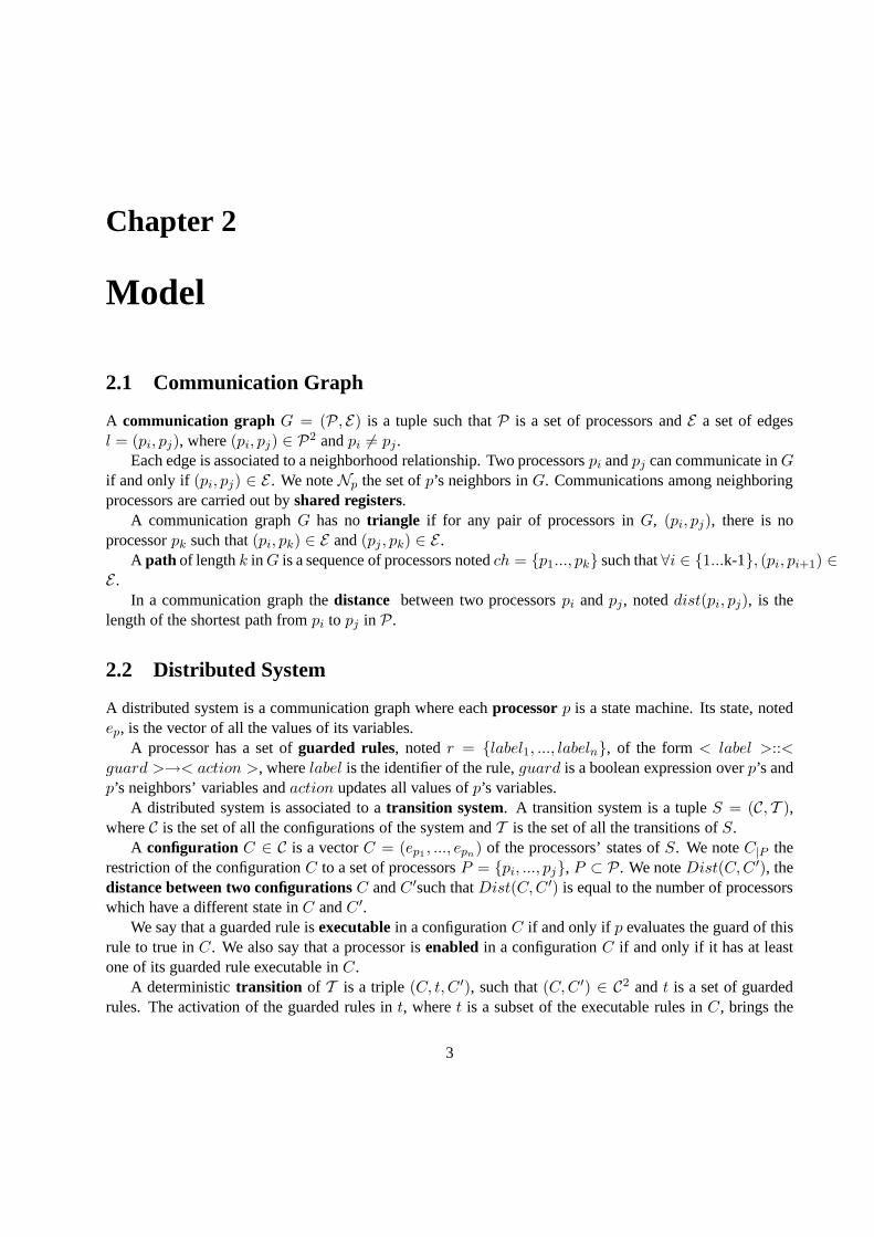
system in the configurationC ′.Thus in the deterministic systems transitionsT = (C, t, C ′) are completely defined by the starting

configurationC and the set of actionst executed inC.

Figure 2.1: A deterministic transitionT = (C, t, C ′)

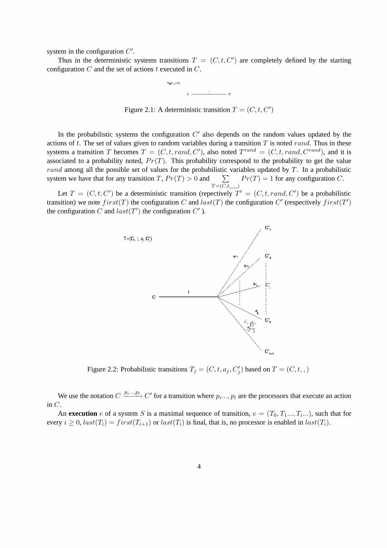
In the probabilistic systems the configurationC ′ also depends on the random values updated by theactions oft. The set of values given to random variables during a transition T is notedrand. Thus in thesesystems a transitionT becomesT = (C, t, rand,C ′), also notedT rand = (C, t, rand,Crand), and it isassociated to a probability noted,Pr(T ). This probability correspond to the probability to get the valuerand among all the possible set of values for the probabilistic variables updated byT . In a probabilisticsystem we have that for any transitionT , Pr(T ) > 0 and

∑

T=(C,t,_,_)Pr(T ) = 1 for any configurationC.

Let T = (C, t, C ′) be a deterministic transition (repectivelyT ′ = (C, t, rand,C ′) be a probabilistictransition) we notefirst(T ) the configurationC andlast(T ) the configurationC ′ (respectivelyfirst(T ′)the configurationC andlast(T ′) the configurationC ′ ).

Figure 2.2: Probabilistic transitionsTj = (C, t, aj , C′j) based onT = (C, t, , )

We use the notationCpi...,pl−−−−→ C ′ for a transition wherepi..., pl are the processors that execute an action

in C.An executione of a systemS is a maximal sequence of transition,e = (T0, T1..., Ti...), such that for

everyi ≥ 0, last(Ti) = first(Ti+1) or last(Ti) is final, that is, no processor is enabled inlast(Ti).

4

Figure 2.3: Execution in the deterministic model

2.3 Demons

The set of possible transitions of the system is restricted by the demon. A demon is a predicate over theexecutions of the system. It chooses for each transitionT = (C, t, C ′) the sett of executed actions amongall the executable actions.

The distributed demon determines, for each transition, any subset of the enabled processors inC toapply at least one of their executable rules. With thesynchronousdemon, in a transitionT ∈ T , all theenabled processors apply one of their executable rules.

2.4 Trees of Executions and Strategies

The following definitions are taken from [Gra00].An execution tree rooted in Cfor a systemS, notedT ree(C), whereC is a configuration ofS, is the

tree-representation of all the executions ofS starting inC (see figure 2.4 and 2.5).

Figure 2.4: Beginning of the execution tree in the deterministic model

A sub-tree of execution of degree1 rooted in C for a systemtS, is a restriction ofT ree(C) such thatfor every node ofT ree(C) either there is no outgoing branch or every possible transition from that nodehas the same labelt (i.e. the same actions are executed).

The interaction between a demon and a distributed system is called astrategie.Let S be a transition system, letD be a demon and letC be a configuration ofS. We call ademon

strategy rooted inC a sub-tree of degree 1 ofT ree(C) such that any execution of the sub-tree verifiesD.Let st be a strategy. Aconeof st corresponding to a non maximal executionh of st, notedConeh, is

the set of all possible executions ofst with the same prefixh. last(h) denotes the last configuration ofh.

5

Figure 2.5: Beginning of the execution tree in the probabilistic model

Figure 2.6: Beginning of a sub-tree of degree1

The number of transitionsT in the historyh is denoted by|h|.In deterministic systems a strategyst is reduced to an execution (cf 2.3).Theprobability measure of a coneCh is the probability measure of the prefixh, that is the product of

the probability of every transition occurring inh. Thus for any strategyst and any coneConeh of st wehavePr(Coneh) > 0.

A coneConeh′ is called asub-coneof Coneh if and only if h′ = [hf ], wheref is an execution factor.We can note that, since that in a probabilistic system we have

∑

T=(C,t,_,_)Pr(T ) = 1 for any configuration

C, we also have for any cone of any strategy∑

|f |=1

Pr(Conehf) = Pr(Coneh).

Figure 2.7: Beginning of a cone

6

2.5 Deterministic Self-Stabilization

The specification of a problem is a predicate over the system executions. The specificationof a staticproblem is a predicate over the system configuration. We calloutput variables of a system, the set ofvariables which have to verify the specification.

LetS = (C,T ) be a transition system andSpe be a specification of a problem. ThenS is self-stabilizingfor Spe if and only if there is a subsetL of configurations ofC, namedlegitimate configurationsof S suchthat:

• Every execution that starts in a configuration ofL verifiesSpe.

• Every execution reaches a configuration ofL.

A silent self-stabilizing algorithmA is a self-stabilizing algorithm such that all the configurationsreached by an execution ofA starting from a legitimate configuration have the same projection on the out-put variables ofA. The legitimate configurations of a silent self-stabilizing algorithm are said to besilentconfigurations.

2.6 Probabilistic Self-Stabilization

The notationx ` Pred means that the elementx of X satisfies the predicatePred defined on the setX .We use the notationEPred to represent the set of executions of a strategyst under a demonD that reaches

a configuration that satisfies the predicatePred. The probability associated toEPred is the sum of theprobability of the conesConeh of st such thath = [h′f ], |f | = 1,¬(last(h′) ` Pred) andlast(f) ` Pred.

A predicatePred is closedfor the executions of a distributed system if and only if whenPred holds ina configurationC, Pred also holds in any configuration reachable fromC.

Let S be a system,D be a demon andst be a strategy satisfyingD. Let C|Pred be the set of all systemconfigurations satisfying a closed predicatePred. The set of executions ofst that reach configurationsC ∈ C|Pred is denoted byEPred and its probability byPr(EPred).

In this paper we study a silent probabilistic algorithm. Thedefinition of self-stabilization for this partic-ular type of algorithms is restricted to the probabilistic convergence definition.

A systemS is self-stabilizing under a demonD for a closed legitimacy predicateL on the systemconfigurations, if and only if in any strategyst of S underD the following condition holds:

• (Probabilistic Convergence) The probability of the set of executions ofst, starting fromC, reachinga configurationC ′, such thatC ′ satisfiesL is 1 . Formally,∀st, Pr(EL) = 1.

2.7 Convergence of Probabilistic Stabilizing Systems

We recall here the theorem of local convergence presented in[Gra00]. This theorem can be used for provingself-stabilization via probabilistic attractors.

Let L1 andL2 be two predicates defined on configurations.L2 is aprobabilistic attractor for L1 in asystemS under the demonD, notedL1 prob L2, if and only if for every strategiest of S underD such thatPr(EL1

) = 1, we havePr(EL2) = 1.

Letst be a strategy,PR1 andPR2 be two predicates on configurations, wherePR1 is a closed predicate.Let δ be a positive probability andN a positive integer. LetConeh be a cone ofst with last(h) ` PR1

7

and letF denote the set of sub-conesConeh′ of the coneConeh such that the following is true for everysub-coneConeh′ : last(h′) ` PR2 and |h′| − |h| ≤ N . The coneConeh satisfies the property oflocalconvergencefrom PR1 to PR2, notedLC (PR1, PR2, δ,N), if and only if Pr(

⋃Coneh′∈F Coneh′) ≥ δ.

Theorem 2.7.1 Let st be a strategy of the systemS under the demonD. Let PR1 be a closed predicateon configurations such thatPr(E1) = 1. Let PR2 be another closed predicate on configurations andPR12 = PR1 ∧ PR2. If ∃δst > 0 and ∃nst > 1 such thatst verifiesLC(PR1, PR2, δst, nst) thenPr(EPR2

) = 1.

2.8 1-adaptivity

In this paper we introduce the new notion of 1-adaptivity, asfollow.A deterministic self-stabilizing algorithmA is 1-adaptive if and only if there is a subset of legitimate

configurations called stable configurations, notedSC, such that:

• (Correction) For any pair of configurations(C,C ′) such thatC ∈ SC, C ′ 6∈ L andDist(C,C ′) = 1,we have, for everyC ′′ such thatC ′ → C ′′, C ′′ ∈ L.

• (Convergence) Every execution ofA reaches a configuration ofSC.

• (Closure) Every execution that starts in a configuration ofSC reaches only configurations ofSC

A probabilistic self-stabilizing algorithmA executed by a systemS under a demonD is 1-adaptive ifand only if there is a subset of legitimate configurations called stable configurations, notedSC, such that:

• (Correction) For any pair of configurations(C,C ′) such thatC ∈ SC, C ′ 6∈ L andDist(C,C ′) = 1,we have, for everyC ′′ such thatC ′ → C ′′, C ′′ ∈ L.

• (Probabilistic Convergence) Every strategyst of S underD starting in a configurationC verifies thatthe set of executions inst that reach a configuration ofSC, notedECS has a probability 1. Formally,∀st, Prst(ECSst) = 1.

• (Closure) Every execution that starts in a configuration ofSC reaches only configurations ofSC.

2.9 Balls and Views

In this article we use the concepts ofBall andV iew inspired by those presented in [BDDT98].Let G be a communication graph,d an integer andp a processor ofG, Ball(p, d) is the setB of nodesb

of P such thatdist(p, b) ≤ d. TheviewVdp (C) at distanced of the processorp in a configurationC contains

the state of the processors ofBall(p, d) in C, Vdp (c) = C|Ball(p,d). We use sometimes the term ofBall in a

configurationC instead of viewV1p(c), also notedC|p∪N (p).

A correctview Vdpi

(C) for a self-stabilizing algorithmA, in a transition systemS, is a view such thatthere exists a legitimate configurationl ∈ L of S in which there is a processorpj such thatVd

pi(C) = Vd

pj(C).

Let B be theBall(p, 1), we say thatB is enabled in a configurationC if and only if p is enabled inC.We will also say thatV1

p (C) is enabled.A self-stabilizing algorithm is1-local if and only if every configurationC that only contains correct

views at distance 1 is legitimate.

8

A self-stabilizing algorithm isstrictly 1-local if it is 1-local and if for any configurationC containing aprocessorpi whose view at distance 1 is not correct, then there is a processorpj , neighbor ofpi, whose viewis also incorrect.

9

Chapter 3

Necessary and Sufficient Conditions for1-adaptivity

We consider here 1-adaptive algorithms such thatSC = L. As soon as the system reaches a legitimateconfiguration, it gains the ability to correct a memory corruption in just one transition. The 1-adaptivealgorithms have, under this assumption, the capacity to reach a legitimate configuration in only one transitionfrom an illegitimate configuration at a distance 1 from a legitimate configuration.

Thus, once stabilization is reached and if the faults are separated in space, the only enabled processorsare processors that can correct the system state and there will not be inopportune propagation of erroneousvalues and incorrect behaviors due to faults. This propertymakes the self-stabilizing systems much safer.

We study here the feasibility of such algorithms. For that, we establish some necessary and sufficientconditions for a self-stabilizing algorithm to be 1-adaptive.

For the sake of generality, we choose as the execution model the distributed demon [Dol00].First we will consider strictly 1-local algorithms designed for specific network topologies. The hypoth-

esis of 1-locality is easy to understand: if the algorithm isnot 1-local, from an illegitimate configurationsuch that every view at distance 1 is correct, it is almost notpossible to reach a legitimate configuration inone step. In a second step we will consider any topology but wewill restrict our study to algorithms whoselegitimate configurations are not too close one to the other,in order to be able to determine with certaintywhich is the nearest legitimate configuration.

3.1 Networks without triangle

The networks we consider in this section have no triangles. We make this assumptions for technical reasons,but it should be noticed that several common topologies havethis property (rings, trees, grid, hypercubes,etc.). The corruption of a single processor in a stable legitimate configuration of a self-stabilizing algorithmmay put the system into an illegitimate configuration where potentially several processors can be activated.Then for being an 1-adaptive algorithm any combination of rules must bring the system back into a legitimatestate.

Definition 3.1.1 LetA be a strictly 1-local self-stabilizing algorithm executedon a communication graphGwithout triangle, with associated transition systemS, under the distributed demon. For allpi ∈ P, ∀C ∈ L,C ′ 6∈ L such thatC|pi 6= C ′

|piandC|P\pi = C ′

|P\pi. Let:

10

• Condition 1 (Locality) No processorpj with a correct viewV1pj

(C ′) is enabled inC ′.• Condition 2 (Correction) Any transition ofS fromC ′ implying only processorspj located inB =

Ball(pi, 1) brings the system into a configurationC ′′ such that all the viewsV1pj

(C ′′) are correct.

Proposition 3.1.1 Condition 1∧ Condition 2 is a necessary and sufficient condition for an algorithm to be1-adaptive.

Proof : First, let us proveCondition1 ∧ Condition2 ⇒ 1-adaptive.Let C andC ′ be two configurations ofS such thatC ∈ L, C ′ 6∈ L, Dist(C,C ′) = 1 andC|p 6= C ′

|p.The view at distance 1 inC and inC ′ which are not centered on a processor ofBall(pi, 1) are iden-

tical and thus correct sinceC is legitimate. FromCondition1, only the balls centered on a processor ofBall(pi, 1) with an incorrect associated view inC ′ are possibly enabled. However as A is self-stabilizing,then at least one processor is enabled inC ′.

ThenCondition2 implies that any step taken by the algorithm makes correct all the view centered in aprocessor ofBall(pi, 1) and thus that any transition of the algorithm starting fromC ′ brings the system ina configurationC ′′ where for allp ∈ P,V1

p (C ′′) is correct.C ′′ is thus legitimate sinceA is strictly 1-local.We can conclude thatCondition1 ∧ Condition2 ⇒ 1-adaptive.

Let us prove now1-adaptive⇒ Condition1∧Condition2 and thus¬Condition1∨¬Condition2 ⇒¬1-adaptive. First, if Condition1 is false, then there is at least oneB = Ball(p, 1) enabled inC ′ with acorrect associated viewV1

p(C ′).Moreover asC ′ is illegitimate and the algorithm is strictly 1-local then there are two neighbors pro-

cessorspj andpk such thatV1pj

(C ′) andV1pk

(C ′) are not correct. Since the system has a topology withouttriangle then ifpj ∈ N (p) (respectivelypk ∈ N (p)) thenpk 6∈ N (p) (respectivelypj 6∈ N (p)).

Thus the system may only activateB because we are under the distributed demon. It comes that ina configurationC ′′ where at leastV1

pj(C ′′) or V1

pk(C ′′) is not correct. Because if onlyB is activated in

C ′ then from what precedes eitherpj 6∈ N (p) or pk 6∈ N (p) and thus eitherV1pj

(C ′) = V1pj

(C ′′) orV1

pk(C ′) = V1

pk(C ′′). Moreover because A is strictly 1-localC ′′ is illegitimate and then the algorithm is not

1-adaptive. Thus, we have that¬Condition1 ⇒ ¬1-adaptive.Now if Condition1 is true andCondition2 is false, then there is a transition of the system which pre-

serves an incorrect view and thus leads the system to an illegitimate configuration. In this case the algorithmis not 1-adaptive and we obtain the following implicationCondition1 ∧ ¬Condition2 ⇒ ¬1-adaptive.

We can now conclude that¬Condition1 ∨ ¬Condition2 ⇒ ¬1-adaptive.2

These conditions show that to study the property of 1-adaptivity of strictly 1-local self-stabilizing al-gorithms, it is unnecessary to study all the executions of the system (but just the possible transitions ofthe faulty processor and its neighbors in the configurationsat distance 1 from a legitimate configuration,becauseonly these processors can correct the error).

We can note that the hypothesis of the distributed demon makes theCondition2 difficult to obtain.Indeed the condition implies that all the enabled processors ofBall(pi, 1) must, if they are activated, correctthe error. Then, if several processors are enabled at the same time, their activations must be compatible.

Thus for an algorithm being 1-adaptive under the distributed demon, it is necessary for a processorneighbor ofpi to be enabled if and only if :

• Its activation corrects the error.

11

• This activation is compatible with the activation of any of its enabled neighbors.

We can derive a useful property from proposition 3.1.1.

Proposition 3.1.2 Let A be a 1-adaptive self-stabilizing algorithm, strictly 1-local, executed on a networkwithout triangle, under the distributed demon. If in a givenlegitimate configuration, there exist two proces-sorsp1 andp2 such thatdist(p1, p2) ≥ 3 and whose corruption can lead to an illegitimate configuration,then this configuration is silent.

Proof : Let C ∈ L, p1 andp2 be two processors,dist(p1, p2) ≥ 3, such that there existC1 andC2 suchthat fori ∈ 1, 2 Ci 6∈ L, C|P\pi = Ci

|P\piandC|pi 6= Ci

|pi.

By definition ofCi, for all p such thatdist(p, pi) ≥ 2, we haveV1p (Ci) = V1

p (C). SinceC is legitimateV1

p (Ci) andV1p (C) are correct. Since the algorithm verifies condition 1 of proposition 3.1.1,V1

p (Ci) iscorrect and enabled and thusV1

p(C) is enabled.Then for everyp and everyi ∈ 1, 2such thatdist(p, pi) ≥ 2,V1

p (C) is enabled.By the triangular inequality, and by the choice ofp1 and p2 we have, for allp ∈ P, dist(p, p1) +

dist(p, p2) ≥ dist(p1, p2) > 2. As the distances are positive integers and by virtue of the inequality weobtain that, for allp ∈ P there existsi ∈ 1, 2 such thatdist(p, pi) ≥ 2. But for everyp there existi ∈ 1, 2 such thatdist(p, pi) ≥ 2. ThenV1

p (C) is not enabled and we obtain that no rule is applicable inC. ThusC is a silent configuration.2

We get the following corollary :

Corollary 1 An algorithm which verifies proposition 3.1.2 for all its legitimate configurations is silent.

Proof : It is obvious that if all the legitimate configurations of an algorithm verify 3.1.2 then all of itslegitimate configurations are silent and by definition the algorithm itself is silent.2

For a large majority of self-stabilizing algorithms, the corruption of any of its processors brings thesystem in an illegitimate configuration. Then for the strictly 1-local algorithms, 1-adaptivity is stronglyrelated to the property to be silent.

3.2 Example : 1-adaptive algorithm for a network without tri angles

We present in this section a very simple 1-adaptive self-stabilizing coloration algorithm. A distributed sys-tem is in a configuration that satisfies the coloration problem if and only if all the processors are colored andevery processor has a color different from its neighbors. This algorithm colors a chain of three processors.These three processors are named and thus distinguishable.We name themp1, p2 andp3 wherep1 andp3

are both neighbors ofp2.The system is in a legitimate configuration if and only if it satisfies the coloration specification.

Proposition 3.2.1 Algorithm 3.2 is self-stabilizing for the coloration problem.

Proof :

12

Algorithm 1 Coloration algorithm for a chain of three processors

p1’s variable : p2’s variable : p3’s variable :Color : integer, Color = 0 ; Color : integer, Color∈ 1,2; Color : integer, Color∈ 2,3;p1’s action : p2’s action : p3’s action :TRUE→ ∅; Color =p3.Color→ Color := 1 ; Color =p2.Color→ Color := 3 ;

Closure Let us suppose that the system is in a legitimate configuration , then all the processors have a colordifferent from each other. Thusp2 evaluatesColor = p3.Color to false andp3 evaluatesColor = p2.Coloralso to false. Asp1 cannot change its color, we obtain that no processor can execute an action and changeits color. The system cannot make any transition and thus it remains in a legitimate configuration. The setof the legitimate configurations is closed.

Convergence The only illegitimate configuration of the system is the configuration wherep2 andp3 havethe same color. In factp1 can only have the color 1 which is necessarily different fromthat of its neighborsp2 sincep2 can not get the color 1.

The only color thatp2 andp3 can have in common is the color 2. Thus the only illegitimate configurationis Ci = p1.Color = 0, p2.Color = 2, p3.Color = 2. In this case bothp2 andp3 can execute their action.Since the execution of the action ofp2 or p3 gives to this processor a color that the other cannot have thesystem necessarily get into a legitimate configuration in any transition starting fromCi. 2

Proposition 3.2.2 This algorithm is 1-adaptive.

Proof : Algorithm 3.2 is strictly 1-local and is executed on a chain which by definition contains no triangle.Thus it suffices to checkConditions1and2 from proposition 3.1.1.

Condition1 is actually verified, since if a processor has a correct view then its neighbors have a differentcolor and thus ifp2 has a correct view at distance 1 then it evaluatesColor = p3.Color to false. Ifp3 hasa correct view at distance 1 then it evaluatesColor = p2.Color to false. Asp1 cannot change its color, weobtain that this algorithm verifiesCondition1.

Let us check now thatCondition2 is also satisfied. There is only one illegitimate configuration, theconfigurationCi. This configuration is 1 distant of at least one legitimate configuration since we just haveto change either the color ofp2 or the color ofp3 to reach a legitimate configuration.

In this configuration, two balls are enabled,B1 = Ball(p2, 1) andB2 = Ball(p3, 1). There are threepossible transitions. In the first onlyp2 executes its action. In this casep2 takes color 1 and the system getsinto the configurationC1 = p1.Color = 0, p2.Color = 1, p3.Color = 2, where all the balls are correctand thusCondition2 is satisfied. With the transition where onlyp3 executes its action, the system reachesC2 = p1.Color = 0, p2.Color = 2, p3.Color = 3. Finally if p2 andp3 are activated at the same timethen the system reaches the configurationC3 = p1.Color = 0, p2.Color = 1, p3.Color = 3 and thistransition also satisfiesCondition2. Thus algorithm 3.2 is 1-adaptive.2

3.3 Restriction on the legitimate configuration density

Corollary 1 confirms the impossibility result of [GT02] and points out the connexion between 1-adaptivityand the property to be silent. Let us remind that in [GT02] they prove that any dynamic global algortihmthat tolerates at least one memory corruption requires at leastΩ(D) transitions to converge, whereD is

13

the diameter of the system. We study now the conditions for silent algorithms to be 1-adaptive. We as-sume that self-stabilizing algorithms we consider here have legitimate configurations at distance at least 3from each other. This hypothesis is verified by many algorithm solving problems with only one legitimateconfiguration, such that the computation of the network size, the topology learning, the leader election, etc.

Definition 3.3.1 Let A be a silent self-stabilizing algorithm andL its legitimate configurations, such thatfor all (l, l′) ∈ L2Dist(l, l′) ≥ 3.

Then for allpi ∈ P, ∀C ∈ L, C ′ 6∈ L such thatC|pi 6= C ′|pi

andC|P\pi = C ′|P\pi

. Let:

• Condition 1 (Locality) The only enabled processor inBall(pi, 1) is the processorpi.• Condition 2 (Correction) The activation ofBall(pi, 1) in C ′ bringspi back in the stateC|pi

.

Proposition 3.3.1 Condition 1∧ Condition 2 is a necessary and sufficient conditions forA to be 1-adaptive.

Proof: First we prove the implicationCondition1 ∧ Condition2 ⇒ 1 − adaptive.In C ′ all the viewsV1

p(C ′) such thatp ∈ P \ pi ∪ N (pi) are correct sinceV1p(C ′) = V1

p (C) andCis legitimate. BecauseA is silent any processor with correct view at distance 1 is notenabled. We obtainthat inC ′ only the processors with an incorrect view are potentially enabled. Thus only the processors ofBall(pi, 1) are potentially enabled. According toCondition1 the only enabled ball inC ′ is Ball(pi, 1).Moreover according toCondition2, the activation of this ball putspi in the same state as inC. We canconclude that the only possible transition fromC ′ is the transitionC ′ pi

−→ C where by assumptionC ∈ Land thusA is 1-adaptive.

Let us prove now the reciprocal:1 − adaptive ⇒ Condition1 ∧ Condition2. For that, as for thepreceding conditions, we will prove that¬Condition1∨¬Condition2 ⇒ ¬1− adaptive. Let us supposethatCondition1 is false. As previously, inC ′ all the viewsV1

p (C ′) such thatp ∈ P \pi ∪N (pi) are correctsinceV1

p(C ′) = V1p (C) andC is legitimate. Thus¬Condition1 implies that∃pj 6= pi, pj ∈ N (pi) such

thatV1pj

(C ′) is not correct andBall(pj, 1) is enabled inC ′. Since we are under the distributed demon the

system may perform the transitionC ′ pj−→ C ′′, whereDist(C ′, C ′′) = 1 andC ′

|pj6= C ′

|pj. We thus obtain

that Dist(C,C ′′) = 2. However by assumptionC is legitimate and all the legitimate configurations areseparated by a distance of least 3. ThusC ′′ is not legitimate and we have a transition fromC ′ which bringsthe system into a legitimate configuration. Finally we have¬Condition1 ⇒ ¬1 − adaptive.

Let us consider now thatCondition1 is true andCondition2 is false. Then we know that the onlyenabled ball isBall(pi, 1) and thatC ′ pi−→ C ′′ with C ′′ such thatC ′′

|pi6= C|pi

andC ′′|P\pi

= C ′|P\pi

= C|P\pi.

ThusDist(C,C ′′) = 1, and by assumptionC is legitimate. Because the legitimate configurations are atleastat distance 3 from each other,C ′′ is not legitimate and thenCondition1∧Condition2¬ ⇒ ¬1−adaptive.We conclude that¬Condition1∨¬Condition2 ⇒ ¬1−adaptive and that by consequence1−adaptive ⇒Condition1 ∧ Condition2. 2

The results of this section point out the fact that, if the legitimate configurations (of a silent self-stabilizing algorithm) are at distance at least 3, then the only way to be 1-adaptive is to return after asingle corruption to the previous legitimate configuration. That yields a general methodology for designing1-adaptive algorithms.

• Increase the memory space of the processor for moving away the legitimate configurations.

• Manage for the corrupted processor to be the only one enabled.

14

3.4 Example : 1-adaptive naming algorithm withN -Distant legitimate con-figurations

In this section we describe a probabilistic 1-adaptive self-stabilizing algorithm for the naming problem on acomplete network of sizeN . This algorithm has its legitimate configurations at distanceN from each other.It is well known that naming can not be achieved in a deterministic way. Thus the only known solutions areprobabilistic. That is the case for the algorithm we present, which is also 1-adaptive.

This algorithm works on complete graphs. We assume that eachprocessor has previously numbered itsregisters 1,2,..,N − 1 . We noteReg[i] the value of theith register. Ifp has a neighborq, corresponding toits ith register , thenp can read the number thatq has for the register corresponding top with the functionGetOrder(Reg[i]). This function returnsj if p corresponds to thejth register ofq. The numbering ofregisters can not be corrupted.

3.4.1 Algorithm description

Each processor executing this algorithm has four variables, Name, Names, Snapshot and Reg. ThevariableName represents the name of the processor, the variableNames is an array used to collect theName of the neighbors of the processor. Theith entry inNames corresponds to the register numberedi.The variableSnapshot is an array containing a view of the system configuration.

Finally Reg is an array and it contains at the indexi the shared variable values of the neighbor corre-sponding to theith register. Reg is completely updated before the evaluation of the guarded actions.

A legitimate state is defined as follows. Every pair of processors (p, q) whereq corresponds to theith register ofp, is such thatp.Name 6= q.Name, p.Names[i] = q.Name and p.Snapshots[i] =(q.Name, q.Names).

The principles used for this algorithm are inspired by the local stabilizer of [AD97]. Our goal is toenlarge the system state with copies of each processor stateon each node of the network thanks to thevariablesNames andSnapshot, in order to get the property of N-Distant legitimate configurations. Then,after the corruption of a single processor, the nearest legitimate state is determined. This example illustrateshow the necessary and sufficient conditions we gave, can be used for designing 1-adaptive algorithms.

Stabilization is in two phases. The first one is probabilistic, and put the system either into a correctlynamed configuration (theName variable are all different but theNames andSnapshots variables are notnecessary consistent) or into an illegitimate configuration at distance 1 from a legitimate one. To do this,every processor that has at least one neighbor with the sameName picks up a randomName (action A1or A2), among the set of names not yet attributed. These probabilistic actions lead with probability 1 to aconfiguration where only deterministic actions are possible.

The second phase is deterministic. It either corrects in oneaction the state of a single faulty processor(action A5), or it updates the variablesNames andSnapshot (action A3 and A4).

The 1-adaptive property is obtained by ensuring that in the case of a single corruption there is only oneenabled action (only the faulty processor is enabled). A single corruption leads the system into a configu-ration where only deterministic actions are possible. If the single fault does not corrupt theName variableof the faulty processor only actions A3 or A4 are possible andthe faulty process returns in the correct con-figuration by updatingNames andSnapshot variables. If the single fault corrupts theName variable ofthe faulty processor, the functions(N -1)ConsistentSnapshots andConsensus are used for fault con-finement. Indeed in this case, as theN − 1 correct processors evaluate(N -1)ConsistentSnapshots totrue, they are not enabled. The faulty processor evaluates(N -1)ConsistentSnapshots to false and applies

15

A5. The faulty processor updates itsName variable with value computed by the consensus function andupdates itsNames andSnapshot values. These new values are consistent with theNames andSnapshotvariables of the correct processors.

Algorithm 2 Naming Algorithm for complete networks

VariablesName : integer∈ 0...N -1;Snapshot :array of(Name,Names) of sizeN -1;Names: integer array of sizeN -1;

FunctionsTakeSnapshot :∀i ∈ 0...N -1, Snapshot[i] := (Reg[i].Name,Reg[i].Names);GetNewName : returnsrandom(0, ..., N -1 \ Reg[i].Name|i ∈ 1...N -1 ∧ ∀k ∈ 1...N -1,Reg[i].Name 6= Reg[k].Name);ConsistentSnapshot : returns(∀i ∈ 0...N -1, Snapshot[i] = (Reg[i].Name,Reg[i].Names));(N -1)ConsistentSnapshots :if the Snapshot of p is consistent with theSnapshot of (N -2) of its neighbors and theseSnapshot repre-sent a legitimate configurationreturns trueelsefalse;Consensus :if theSnapshot of the(N -1) neighbors ofp are consistent with each other and theseSnapshots representa legitimate configuration where(p.Name, p.Names) 6= Reg[i].Snapshot[GetOrder(Reg[i])] for all i∈ 0...N -1 thenreturns Snapshot[GetOrder(Reg[1])]; else0;

ActionsA1 : ∃(i, j, k) ∈ 1...N -13, j 6= k, (Name = Reg[i].Name ∧ Reg[j].Name = Reg[k].Name)→ GetNewName;A2 : ∀(i, j) ∈ 1...N -12, Reg[i].Name 6= Reg[j].Name ∧∃k ∈ 1...N -1, Name = Reg[k].Name∧¬(N -1)ConsistentSnapshots ∧Consensus = 0→ GetNewName;A3 : ∀(i, j) ∈ 1...N -12, i 6= j, Reg[i].Name 6= Name ∧ Reg[j].Name 6= Reg[i].Name∧∃k ∈ 1...N -1, Names[k] 6= Reg[k].Name→ ∀i ∈ 1...N -1, Names[i] := Reg[i].Name, TakeSnapshot;A4 : ∀(i, j) ∈ 1...N -12, i 6= j, Reg[i].Name 6= Name ∧ Reg[j].Name 6= Reg[i].Name ∧ ∀k ∈1...N -1, Names[k] = Reg[k].Name ∧ ¬ConsistentSnapshot∧ ¬(N -1)ConsistentSnapshots→ TakeSnapshot;A5 : ∀(i, j) ∈ 1...N -12, Reg[i].Name 6= Reg[j].Name ∧∃k ∈ 1...N -1, Name = Reg[k].Name∧Consensus 6= 0→ Name = Consensus.Name, Names = Consensus.Names, TakeSnapshot;

3.5 Algorithm Analysis

Definition 3.5.1 A legitimate configuration for algorithm 3.4.1 is such that for every pair of processors(p, q) whereq corresponds to theith register ofp, p.Name 6= q.Name, p.Names[i] = q.Name andp.Snapshots[i] = (q.Name, q.Names).

16

Proposition 3.5.1 The legitimate configurations of algorithm 3.4.1 are N-Distant.

Proof : In any two different legitimate configurations, notedL1 andL2, there are at least two differentprocessors, notedp andq, such thatL1|p.Name 6= L2|p.Name andL1|q.Name 6= L2|q.Name. Infact if every processor has the sameName thenL1 = L2, and if one processorp has a differentNamein L1 andL2 then has there are onlyN possibleName for theN different processor there is at least theprocessorq that had theName, L2|p.Name in L1 which necessary has a newName in L2.

Then every processorr different fromp andq, for whichp is theith neighbor andq thejth neighbor, issuch thatL1|r.Names[i] 6= L2|r.Names[i] sinceL1|r.Names[i] = L1|p.Name, L2|r.Names[i] =L2|p.Name andL1|p.Name 6= L2|p.Name. Thus we haveL1|r 6= L2|r.

SinceL1|p.Name 6= L2|p.Name andL1|q.Name 6= L2|q.Name, we haveL1|p 6= L2|p andL1|q 6= L2|q. Then we can conclude that every processor has a different state inL1 andL2. ThusL1 andL2

are at distanceN from each other.The legitimate configurations of this algorithm are N-Distant.2

Definition 3.5.2 We say that a processorsp in a configurationC of a distributed systemS that executesalgorithm 3.4.1 ismisnamed (or wrongly named) if and only if there is a processorq in S such thatC|p.Name = C|q.Name. We also say thatp andq are homonyms.

Definition 3.5.3 Let P (k) be a predicate over the configurations of a systemS executing algorithm 3.4.1.A configurationC of S satisfiesP (k) if and only if there is exactelyk different misnamed processors inC.

First we prove that there is no possible way to misnammed a processor. Thus the number of misnammedprocessor in the system can only decrease.

Proposition 3.5.2 LetS be a system that executes algorithm 3.4.1. There is no transition T = (C, t, rand, C ′)of S such thatC ` P (k1), C

′ ` P (k2) andk2 > k1.

Proof : In any configurationC of the system, the processors that can change theirName are the proces-sors that can execute A1, A2 or A5. Those processors necessarily have at least one neighbor with the sameName, otherwise they evaluate the guards of these rules to false.However none of these actions can givea Name that a correctly named processor has before the transition.In fact A1 and A2 use the methodGetNewName that picks up uniformly a randomName in the set(0, ..., N -1 \ Reg[i].Name|i ∈1...N -1 ∧ ∀k ∈ 1...N -1, Reg[i].Name 6= Reg[k].Name). Thus those processors cannot be mis-named after the execution ofA1 or A2.

Moreover A5 can not give theName that a processor had before the transition otherwise the methodconsensus would return 0. Thus it can have the sameName as a processor that has been activated duringthe same transition. In this case this processor was alreadywrongly named.2

Proposition 3.5.3 Every coneConeh of every strategyst of a systemS that executes algorithm 3.4.1 underthe distributed demon, such thatlast(h) satisfiesP (k), for a k ≥ 3, satisfiesLC(P (k), P (k − 1), δk, 1),whereδk > 0.

17

Proof : Let st be a strategy of algorithm 3.4.1 under the distributed demonstarting in a configurationCandConeh be a cone ofst, whereC ′ = last(h) satisfiesP (k) for a k ≥ 3. We have by definition thatPr(Coneh) > 0 sinceConeh is a cone ofst.

From proposition 3.5.2 we know that every configuration reachable fromC ′ in st verifiesP (k′) fork′ ≤ k. Moreover the only action that can be executed inC ′ is action A1. Thus in every possible transitionof st starting inC ′ there is a non empty subset of misnamed processors of the system, notedWN , that areactivated to execute their action A1.

Then the probability, for the system to reach a configurationC ′′ where there is at least 1 less misnammedprocessor, is equal to the probability of a transition whereone of the misnamed processors get a correctName. This means that this processor is activated and it picks up aName different from all theName ofthe not activated processors. ThisName also has to be different from the newName chosen by the otheractivated processor.

Let Coneh′ be a cone ofst whereh′ = [hf ], |h′| = |h| + 1, last(h′) = C ′′ and last(h′) satisfiesP (k − 1) andT = (C ′, t, rand, C ′′) be a transition inh′ as described above. Letm be the number ofdifferentName of not correctly named processors that are not activated inT , (k/2) ≥ m ≥ 0, since everymisnammed processor has at least one homonym.

The probability associated toT is :Pr1 = probability to pick up aName that none of the not activated processor has

= (k − m)/kPr2 = probability that every other processors picks up aName different from the processor

that get a correct Name= ((k − (m + 1))/k)|WN−1|

Pr3 = Pr1 ∗ Pr2

Pr3 = (k − m)/(k) ∗ ((k − (m + 1))/k)|WN−1|

We get thatPr3 > 0 sincek ≥ 2m. Thus we have that from any configurationC of the system,where there is at more than two misnamed processors. There isat least one transition fromC that leads ina configuration where there is one less misnamed processor that is associated positive probability. Then weobtaine that the union of the sub-cones ofConeh that reache a configuration with one less misnamed proces-sor is superior or equal to the probability calculated above. FormalyPr(

⋃Coneh′ ,∈F ,|h′|=|h|+1 Coneh′) ≥

Pr(Coneh′) = Pr(Coneh) ∗ (k − m)/(k) ∗ ((k − (m + 1))/k)|WN | = δk > 0. 2

Proposition 3.5.4 Every strategyst of a systemS that executes algorithm 3.4.1 under the distributed demonverifiesPrst(EP (2)) = 1.

Proof : Let st be a strategy under the distributed demon rooted inC. If C ` P (k), k ≤ 2 then the propertyis trivially verified.

If C ` P (k), k ≥ 2 then we know from proposition 3.5.3 and 3.5.3, and theorem 2.7.1 thatPst(EP (k−1)) =1. By induction onk we get thatPst(EP (2)) = 1. 2

Proposition 3.5.5 In any strategyst of a systemS that executes algorithm 3.4.1 under the distributeddemon, every coneConeh such thatlast(h) = Ci, Ci 6∈ L and Ci ` P (2), and for every legitimateconfigurationL, Dist(L,Ci) ≥ 2. Then either the system reaches in one transition a configuration whereevery processor has an uniqueName or Coneh verifiesLC(P (2), P (0), δ, 1) for δ > 0.

18

Proof : Let Coneh be a cone of a strategyst of a system executing algorithm 3.4.1 under the distributeddemon. LetCi = last(h) be an illegitimate configuration such thatCi ` P (2), so there exists two proces-sors inCi with the sameName, namelyp andq, andCi is also such that for every legitimate configurationL ∈ L, Dist(L,Ci) ≥ 2.

In Ci no processor different fromp andq can execute an action. In fact they cannot execute A2 or A5as they are correctly named. They can not execute A1, A3 or A4 as there is exactly two processors with thesameName in the network. Thus the only enabled processors inCi arep andq.

For the same reason,p andq can not execute A1,A3 or A4. Then they can just execute A2 or A5. Theycan not both evaluate the guard of A5 to true since that would mean that they both evaluate Consensus totrue. And so they have a different state from the one in theSnapshot of their neighbors at the index thatcorrespond to them (which are different by definition). But Consensus is evaluated to 0 for a processorif there is aSnapshot of one of its neighbor which contains more than one state thatdoes not match thecurrent state of a processor. Here this is the case for every processor different fromp andq. Thus there is atmost one processor inCi that evaluates the guard of A5 to true.

Suppose thatp evaluates A5 to true. The first possibility is that in the transition starting fromCi, justpis activated. Then the system reaches in one transition a configuration where every processor has a uniqueName, since Consensus can not return a value with aName already attributed.

Otherwise the system takes a step whereq is activated. Ifq is activated, then there is two possibilities :p is also activated or justq is activated.

Let Coneh′ be a sub-cone ofConeh in st, such thath′ = [hf ], last(h′) = C ′′, |h| + 1 = |h′| and forevery pair(pi, pj) of P2, C ′′

|pi.Name 6= C ′′

|pj.Name.

Let Pr(Coneh) be the probability associated toConeh.If just q is activated inlast(h), thenConeh′ exists since it corresponds to the transition ofst from

last(h) whereq picks up the lastName that no processor has. Sinceq uniformly randomly chose aNamein the set ofName corresponding to itsName in last(h) and theName ∈ 0...N − 1 that no processorhas inlast(h) (by definition of GetNewName). We get that :

Pr(Coneh′) = 1/2 ∗ (Pr(Coneh))If p andq are both activated inlast(h). Then the coneConeh′ exists since it corresponds to the transition

of st from last(h) wherep executes A5 and changes itsName andq picks up theName it already had inlast(h). Sinceq uniformly randomly chose aName in a set of two values as described above. We get that :

Pr(Coneh′) = 1/2 ∗ (Pr(Coneh))

Suppose now that no processor can execute A5 inCi. Thenp andq are enabled as they evaluate theguard of A2 to true.

If just one processor is activated thenCone′h exists and the probability associated to it inst is :Pr(Coneh′) = 1/2 ∗ (Pr(Coneh)).As it has just been proven.Otherwisep andq are activated inCi. Then there are four possible toss. They both get a newName,

they both keep their formerName or one of the processor changes itsName and the other don’t. Thus theprobability associated toCone′h is :

Pr(Coneh′) = 1/4 ∗ (Pr(Coneh))However as there is two suchCone′h the probability associated to all the sub-cones ofConeh that

satisfiesP (0) is 1/2 ∗ (Pr(Coneh)).

19

We can conclude that either the system reaches in one transition from Ci a configuration where everyprocessor has a uniqueName or Coneh verifiesLC(P (2), P (0), δ, 1) for δ = 1/4 ∗ (Pr(Coneh)) > 0.

2

Proposition 3.5.6 Any transition of a system executing algorithm 3.4.1 under the distributed demon thatstarts in an illegitimate configurationC ′ such thatC ′ ` P (2) and there existsC ∈ L, Dist(C,C ′) = 1brings the system into a legitimate state, namelyC.

Proof : Suppose two configurationsC ∈ L and C ′ 6∈ L such thatC|pi 6= C ′|pi

, C|pi.Name 6=

C ′|pi

.Name andC ′|pi

.Name = C ′|pj

.Name. Then for the same reasons as the one mentioned above.

No processor of the system different frompi andpj is enabled inC ′.SinceC ′ is at distance 1 fromC, all the Snapshot of the processors different frompi are coherent

and all contains the current state of the processors different from pi in the correct order (in regard to theirlocal register order). Thus every processor different frompi evaluates (N -1)ConsistentSnapshots to true.Thenpj cannot execute A2. It can not execute A1, A3 or A4 as there are exactly two processors with thesameName in C ′. It can not execute A5 since it evaluates (N -1)ConsistentSnapshots to true, which meansthat all its neighbors different frompi have its current state in theirSnapshot at the right place and thusConsensus returns 0.

The only enabled processor inC ′ is pi. pi evaluates Consensus to(C|pi.Name,C|pi.Names) sinceeverySnapshot of its neighbors contains this value at the index concerningpi in C and thus inC ′. Then itcan not execute any other actions and the only possible transition of the system starting fromC is C ′ pi−→ C.2

Proposition 3.5.7 Let st be a strategy of a system executing algorithm 3.4.1 under thedistributed demon.Then everyConeh of st such thatlast(h) ` P (0) only contains executions that reach a legitimate configu-ration.

Proof : Let Coneh be a cone of a strategyst of a system executing algorithm 3.4.1 under the distributeddemon such thatlast(h) = C andC ` P (0).

Then by hypothesis and by proposition 3.5.2 we have that, in any configuration reachable fromC, P (0)is satisfied and no processor can execute A1, A2 or A5 inC. Since there are no two processors with thesameName. Thus the only enabled actions are A3 and A4 and no processor can change its variableNameany more. Then the processors just have to fill in correctly their variableNames andSnapshot in order toreach a legitimate configuration. Let us prove now that evry processor will first get a correct value for itsvariableNames. And then a correct value for its variableSnapshot and thus the system necessarily willget in a legitimate configuration.

Let WN be the set of processors that have a wrong variableNames. That is, a variableNames thatdoes not contain theName of each of its neighbors in the order of its registers. Letwn be the number ofprocessors inWN in C. LetWS be the set of processors that have a wrong variableSnapshot. That is, avariableSnapshot that does not contain the tuple(Name,Names) of each of its neighbors in the order ofits register in the current state of the system.

Every processor inWN evaluates the guard of A3 to true. They evaluate the guard of A4 to false sincethey have a wrong variableNames. Every processors inWN ∩ WS only have one action executable,namely A3. Since the processors ofWN can not execute A4.

20

Every processor ofWN chosen by the demon to execute A3 will get a correct variableNames forthe remaining of the execution. Every processor fromWS activeted by the demon is not enabled until aprocessor ofWN is activeted, since after the execution of A4 a processor evaluatesConsistentSnapshotto true until a processor changes either its variableName or its variableNames.

Then every|WS| ≤ N transitions at least one processor ofWN is activated and we have|WN | =wn − 1. In fact even if in every transition of the execution the demon choses only processors inWS it willreach in a number of transition lower or equal to|WS| a configuration where,WS = ∅, and where the onlyenabled processors are the processors ofWN . It will then activate one of those processors and the setWSwill contain all the processors of the system.

But then again in at least|WS| ≤ N transitions we will have|WN | = wn − 2. By induction onwnwe get that the system reaches fromC a configuration whereWN = ∅ in a number of transitions lower orequal town ∗ N .

Then the system only reaches configurations where every processor is correctly named and has a correctvariableNames. In fact the only enabled processors are the processors ofWS. Since in every transition ofthe system there is at least one processor activated then they will all be activated in a number of transitionlower or equal toN . Then everySnapshot will be updated correctly and the system will reach a legitimateconfiguration.

Finally we have that every sub-cone ofConeh reaches a legitimate configuration fromC in at mostN ∗ (wn + 1) transitions.2

Proposition 3.5.8 Algorithm 3.4.1 is 1-adaptive.

Proof : Let C andC ′ be two configurations of a systemS executing algorithm 3.4.1 such thatC ∈ L,C ′ 6∈ L, Dist(C,C ′) = 1,C|pi

6= C ′|pi

.Then if there is a processorpj 6= pi in S such thatC ′

|pj.Name = C ′

|pi.Name then by proposition 3.5.6

we know that the only possible transition fromC ′ is C ′ pi−→ C.

Let suppose now thatC|pi.Name = C ′

|pi.Name andC|pi

.Names 6= C ′|pi

.Names. No processorpj

different frompi is enabled. In fact as there are no two processors with the same Name, no processor canexecute A1, A2 or A5. Since for everypj ∈ P, pj 6= pi, C|pj

= C ′|pj

andC|pi.Name = C ′

|pi.Name, they

all evaluate the guard of A3 to false since they haveC ′|pj

.Names[i] = C|pi.Name 6= C ′

|pi.Name for the

index i corresponding topi and (N -1)ConsistentSnapshots to true, since every processor butone is in thesame state as inC which is a legitimate configuration. Then they can not execute A4 neither.

Thus the only enabled processor inC ′ is pi. SinceC|pi.Names 6= C ′

|pi.Names and every processor

has the sameName in C andC ′, pi evaluates the guard of A4 to true. By the application of this rule pi

regains a correctNames and a correctSnapshot that contains the currentName and state of the processorswhich are the same as inC, since every processor verifiesName.C ′ = Name.C. Thus the only possibletransition starting fromC ′ is C ′ pi−→ C.

Finally we suppose that just theSnapshot of pi is corrupted. Then as previously, the only enabledprocessor ispi and the only executable action forpi is A4. It can not execute A3 any more since its variableNames is correct. Thus the only executable action forpi is A4. Since all the other processors have the samestate as inC, pi regains with A4 the state that it had inC. Then again the only possible transition fromC ′

is C ′ pi−→ C.We can conclude that in any configurationC ′ as described above the only enabled processor ispi and

the only possible transition of the system isC ′ pi−→ C. Thus by proposition 3.3.1 we have that algorithm3.4.1 is 1-adaptive.2

21

Proposition 3.5.9 Algorithm 3.4.1 is silent.

Proof : Suppose that a system that executes algorithm 3.4.1 is in a legitimate configurationC ∈ L.Then no processor can execute actions A1, A2 nor A5 as there isno two processors(p, q) ∈ P2 suchthatCp.Name = Cq.Name. No processor can execute A3 or A5, since by the definition 3.5.1 we knowthat inC, p.Names[i] = q.Name andp.Snapshots[i] = (q.Name, q.Names). Thus when a processorevaluates the guard of A3 and A4 its evaluates∧∃k ∈ 1...N -1, Names[k] 6= Reg[k].Name to false and∀i ∈ 0...N -1, Snapshot[i] = (Reg[i].Name,Reg[i].Names) to true and thus ConsistentSnapshot tofalse. Finally, no processor is enabled inC thenC is terminal and the algorithm is silent.2

Proposition 3.5.10 Algorithm 3.4.1 is self-stabilizing for the predicate of definition 3.5.1.

Proof : From proposition 3.5.4, we have that in any strategyst of a system that executes algorithm 3.4.1under the distributed demon,Prst(EP (2)) = 1.

Then we get thatP (2) is a probabilist attractor for TRUE,TRUE prob P (2).From proposition 3.5.5 and the theorem 2.7.1 of local convergence we have thatP (2) prob P (0). Thus

we haveTRUE prob P (2) prob P (0).Finally from proposition 3.5.7 andTRUE prob P (2) prob P (0) we have that algorithm 3.4.1 is self-

stabilizing for the predicate of definition 3.5.1 and thus for the naming problem.2

Proposition 3.5.11 Algorithm 3.4.1 is a self-stabilizing 1-adaptive silent probabilistic algorithm for thepredicate of definition 3.5.1.

proof From propositions 3.5.11 3.5.9 and 3.5.8 we have that algorithm 3.4.1 is a self-stabilizing 1-adaptivesilent probabilistic algorithm for the predicate of definition 3.5.1.

22

Chapter 4

Conclusion

We have introduced here the new concept of 1-adaptivity for self-stabilizing systems. This concept is pow-erful and interesting since it makes possible to guarantee an almost instantaneous correction of memorycorruptions hitting only one processor of the system. It ensures that the fault is not propagated and thus thatthe non faulty processors are not affected by the corruptionof their neighbors. Note that our results havein fact a larger application domain and there are two simple extensions. First the assumption of a singlecorruption can be slightly relaxed. Our results also apply when an arbitrary number of memory corruptionshit the system, provided that two neighbors are not simultaneously corrupted. If it is not the case, the generalstabilizing mechanisms allow anyway the system to recover (unfortunately in more than one step). Secondlythe results can be extended in a straightforward way to the case where at most k (for a fixed integer k) cor-ruptions hit the system. Analogous sufficient and necessaryconditions can be obtained. They can also bedecided locally.

In conclusion we would like to emphasize the fact that, more than a way for verifying that existing self-stabilizing algorithms are not 1-adaptive (everybody knewthat before), the conditions we presented givea systematical way to design 1-adaptive algorithms. The idea is to enlarge the state of the processes withvariables whose unique role is to realize the necessary and sufficient condition. We presented in the exampleof naming how this idea could be exploited by hand (rule A5), but our approach leads to a more systematicmethod. The goal here is to produce an automatic transformerhaving as an input a self-stabilizing algorithmand producing as an output an equivalent self-stabilizing algorithm, having the supplementary property tobe 1-adaptive (or more generally k-adaptive for any given k). One of the most often cited drawback of self-stabilization is the loss of the safety during the stabilization phase, that makes self-stabilization inadequatefor critical tasks. Our work can be seen as an attempt to overcome this drawback.

23

Bibliography

[AD97] Y. Afek and S. Dolev. Local stabilizer. InIsrael Symposium on Theory of Computing Systems,pages 74–84, 1997.

[AKP03] Y. Azar, S. Kutten, and B. Patt-Shamir. Distributederror confinement. InProceedings of thetwenty-second annual symposium on Principles of distributed computing, pages 33–42, Boston,Massachusetts, July 2003.

[BDDT98] J. Beauquier, S. Delaët, S. Dolev, and S. Tixeuil. Transient fault detectors. InProceedings ofthe 12th International Symposium on DIStributed Computing(DISC’98), number 1499, pages62–74, Andros, Greece, 1998. Springer-Verlag.

[BGK99] J. Beauquier, C. Genolini, and S. Kutten. Optimal reactive k-stabilisation: the case of mutualexclusion. In18th Annual ACM Symposium on Principles of Distributed Computing, May 1999.

[Dij74] E.W. Dijkstra. Self stabilizing systems in spite ofdistributed control.Communications of theACM, 17:643–644, 1974.

[Dol00] Shlomi Dolev.Self-Stabilization. MIT Press, Cambridge, MA, 2000. Ben-Gurion University ofthe Negev, Israel.

[GGHP96] S. Ghosh, A. Gupta, T. Herman, and S.V. Pemmaraju. Fault-containing self-stabilizing algo-rithms. InSymposium on Principles of Distributed Computing, pages 45–54, 1996.

[Gra00] M. Gradinariu.Modélisation vérification et raffinement des algorithmes auto-stabilisants. PhDthesis, Université Paris XI, Orsay, 2000.

[GT02] C. Genolini and S. Tixeuil. A lower bound of dynamic k-stabilization in asynchronous systems.In 21st IEEE Symposium on Reliable Distributed Systems (SRDS’02), pages 212–222, OsakaUniversity, Suita, Japan, Octobre 2002.

[Her97] T. Herman. Observations on time adaptive self-stabilization, 1997.

[KP95] S. Kutten and D. Peleg. Fault-local distributed mending. In Proceedings of the 14th AnnualACM Symposium on Principels of Distributed Computing (PODC’95), August 1995.

[KP97] S. Kutten and B. Patt-Shamir. Time-adaptive self stabilization. InSymposium on Principles ofDistributed Computing, pages 149–158, 1997.

[KP98] S. Kutten and B. Patt-Shamir. Asynchronous time-adaptive self stabilization. InSymposium onPrinciples of Distributed Computing, page 319, 1998.

24

[KP01] S. Kutten and B. Patt-Shamir. Adaptive stabilization of reactive distributed protocols, 2001.

[NA02] M. Nesterenko and A. Arora. Local tolerance to unbounded byzantine faults, 2002.

25

Chapter 5

Annexe

(N -1)SnapshotsCoherents :/* First we check if two processors have two index of theirSnapshot that do not correspond tothe current state of a processor */¬ (∃i ∈ 1...N -1

∃k ∈ 1...N -1(Reg[i].Snapshot[k] 6= (Name,Names)∧∀m ∈ 1...N -1Reg[i].Snapshot[k] 6= (Reg[m].Name,Reg[m].Names)∧∃l ∈ 1...N -1

l 6= k∧Reg[i].Snapshot[l] 6= (Name,Names)∧∀m ∈ 1...N -1Reg[i].Snapshot[l] 6= (Reg[m].Name,Reg[m].Names)

)∧∃j ∈ 1...N -1

(j 6= i∧∃k ∈ 1...N -1

Reg[j].Snapshot[k] 6= (Name,Names)∧∀m ∈ 1...N -1Reg[j].Snapshot[k] 6= (Reg[m].Name,Reg[m].Names)∧∃l ∈ 1...N -1

l 6= k∧Reg[j].Snapshot[l] 6= (Name,Names)∧∀m ∈ 1...N -1Reg[j].Snapshot[l] 6= (Reg[m].Name,Reg[m].Names)

))

/* We check ifp has not two index of its Snapshot that do not correspond to thecurrent state ofa processor */∧ ¬ (∃i ∈ 1...N -1

∀m ∈ 1...N -1Snapshot[i] 6= (Reg[m].Name,Reg[m].Names)∧∃j ∈ 1...N -1

i 6= j

26

∧∀m ∈ 1...N -1Snapshot[j] 6= (Reg[m].Name,Reg[m].Names))

/* We check if all the processors but one have an index in theirSnapshot that allrepresent the same state of a processor that is not the current state of a processor*/∧ ¬ (∃i ∈ 1...N -1

∀m ∈ 1...N -1Snapshot[i] 6= (Reg[m].Name,Reg[m].Names)∧∃j ∈ 1...N -1

∀m ∈ 1...N -1Reg[j].Snapshot[m] 6= Snapshot[i]∧∃k ∈ 1...N -1,

k 6= j∧∀m ∈ 1...N -1Reg[k].Snapshot[m] 6= Snapshot[i]

)/* We check if there is no two processors with twice the sameName in their variableNames.*/∧ ¬ (∃i ∈ 1...N -1

∃j ∈ 1...N -1Reg[i].Names[j] = Reg[i].Name

∨∃k ∈ 1...N -1k 6= j∧Reg[i].Names[j] = Reg[i].Names[k]

)∧∃l ∈ 1...N -1

l 6= i∧∃j ∈ 1...N -1(Reg[l].Names[j] = Reg[l].Name

∨∃k ∈ 1...N -1k 6= l∧Reg[l].Names[j] = Reg[l].Names[k]

))

/* Finally we check if there is no two processors with twoName in their variableNames that correpond not to the currentName of a processor.*/∧ ¬ (∃i ∈ 1...N -1

∃j ∈ 1...N -1(∀m ∈ 1...N -1Reg[i].Names[j] 6= Reg[m].Name∧∃k ∈ 1...N -1

k 6= j∧∀m ∈ 1...N -1Reg[i].Names[k] 6= Reg[m].Name

)∧(∃l ∈ 1...N -1

(l 6= i

27

∧∃j ∈ 1...N -1∀m ∈ 1...N -1Reg[l].Names[j] 6= Reg[m].Name∧∃k ∈ 1...N -1

j 6= k∧∀m ∈ 1...N -1Reg[l].Names[k] 6= Reg[m].Name

))

Consensus :/* First we check if all the Snapshot of the processors different fromp contain the same values */if (∀i ∈ 1...N -1

∀j ∈ 1...N -1∧∀k ∈ 1...N -1

k 6= i∧∃l ∈ 1...N -1

Reg[i].Snapshot[j] = Reg[k].Snapshot[l]∨∃m ∈ 1...N -1Reg[i].Snapshot[j] = (Reg[m].Name,Reg[m].Names)

)/* We check if all the current state of the processors different from p appears in theSnapshot oftheir neighbors different fromp */

∧ (∀i ∈ 1...N -1∀j ∈ 1...N -1

i 6= j∧∃k ∈ 1...N -1

(Reg[i].Name,Reg[i].Names) = Reg[j].Snapshot[k])

/* We check if all the processors different fromp have a variableNames which contain theNameof all their neighbors different fromp */

∧ (∀i ∈ 1...N -1∀j ∈ 1...N -1

i 6= j∧∃k ∈ 1...N -1Reg[i].Name = Reg[j].Names[k])

Reg[i].Name = Reg[j].Names[k])/* Finally we check if all the processors different fromp have the same value in theirSnapshot at theindex correponding to p and this value is different from the current state ofp */∧ (∀i ∈ 1...N -1

∀j ∈ 1...N -1i 6= j

(Reg[i].Snapshot[LireMonOrdre(Reg[i])] 6= (Name,Names)∧Reg[i].Snapshot[LireMonOrdre(Reg[i])] =Reg[j].Snapshot[LireMonOrdre(Reg[j])]))

28