1 a résumé of xed point theorems - dcs.warwick.ac.uksgm/a7-2x2.pdf · 1 a résumé of xed point...

29th Summer Conference on Topologyand it’s Applications

Workshop on fixed points: Theoretical Foundations andapplications in computing and elsewhere

Franz-Viktor Kuhlman1 Steve Matthews2

1Centre for Algebra, Logic and Computation (CALC)University of Saskatchewan, Canada

2Department of Computer ScienceUniversity of Warwick, UK

Download: www.dcs.warwick.ac.uk/~sgm/a7.pdf

1 / 59

Abstract

Banach’s theorem for defining the unique fixed point of a contractionmapping over a complete metric space (1922) has co-existed withTarski’s theorem for computing the least fixed point of an orderpreserving mapping over a complete lattice (1955). These two greattheorems were later unified to define the least fixed point of acontraction mapping over a bottomed chain complete partial metricspace (1992). The challenge now is to continue to say more abouthow this fixed point theorem can be defined in contexts of relevanceto practical computing.

2 / 59

ContentsNon-zero self-distance? You cannot be serious!

1 A résumé of fixed point theorems1.1 What is a fixed point?1.2 Banach’s contraction mapping theorem.1.3 Tarski’s least fixed point theorem.1.4 Non-zero self-distance.1.5 A partial metric fixed point theorem.1.6 A criticism of partial metric spaces.

2 Failure takes time (scalable maths)2.1 Pixels as (consistent) approximations.2.2 The paradox of double negation.2.3 Wadge’s hiaton.2.4 Intensional partial metric spaces.2.5 Conclusions and further work.

"You cannot be serious!"

John McEnroe,mad on Centre Court,Wimbledon 1981.

3 / 59

1 A résumé of fixed point theorems1.1 What is a fixed point?

Initial assumptions:I X is a mathematical structure having at least a set

structure. That is, x ∈ X asserts x is a point (akamember) in X . That is, a membership relation to assertx ∈ X or x 6∈ X , and an equality relation to assert x = y orx 6= y for any x , y ∈ X .

I A function f : X → Y maps each point x ∈ X to aunique point f (x) ∈ Y .

I For each X and f : X → X a point x ∈ X is fixed iff (x) = x .

I X has additional structure(s) (such as a topology τ ⊆ 2X ,or a category) to enrich the study of fixed points.

20th century mathematics gave us two undisputably classicfixed point theorems.

4 / 59

1 A résumé of fixed point theorems1.2 Banach’s contraction mapping theorem

Maurice Fréchet(1878-1973)

Definition (1)A metric space (Fréchet, 1906) is a tuple(X , d : X × X → [0,∞)) such that,

d(x , x) = 0d(x , y) = 0 ⇒ x = yd(x , y) = d(y , x)

d(x , z) ≤ d(x , y) + d(y , z)

Example (1)| · − · | : (−∞,+∞)2 → [0,∞) where |x − y | = x − y ify ≤ x , y − x otherwise.

5 / 59


Definition (2)A topological space is a pair (X , τ ⊆ 2X ) s.t.,

∈ τ and X ∈ τ

∀A, B ∈ τ . A∩B ∈ τ (closure under finite intersections)∀Ω ⊆ τ .

⋃Ω ∈ τ (closure under arbitrary unions)

Each A ∈ τ is termed an open set of the topology τ , andeach complement X − A termed a closed set.

Definition (3)For each topological space (X , τ) a basis of τ is a Ω ⊆ τsuch that each member of τ is a union of members of Ω .

Example (2)The finite open intervals (x , y) are a basis for the usualtopology on (−∞,+∞) .

6 / 59


Definition (4)For each metric space (X ,d) , a ∈ X , and ε > 0an open ball Bε(a) = x ∈ A | d(x ,a) < ε .

Lemma (1)For each metric space (X , d) the open balls form the basis fora topology τd over X .

Example (3)Let d be the metric on the set F ,T of truth values false &true such that d(F ,T ) = 1 . Then τd = 2F ,T ,and F, T is a basis for τd .

7 / 59


Definition (5)For each topological space (X , τ) a sequence x ∈ Xω

converges to a point l ∈ X (known as a (sequential) limit pointof x) if,

∀ A ∈ τ . l ∈ A ⇒ ∃ n ≥ 0 . ∀ m ≥ n . xm ∈ A

Definition (6)A topological space (X , τ) is Hausdorff separable (akaT2 ) if,

a 6= b ⇒ ∃ A,B ∈ τ . a ∈ A ∧ b ∈ B ∧ (A ∩ B = φ)

Thus distinct points in a Hausdorff separable topologicalspace can be separated by disjoint open sets. However inweaker separable spaces limit points of a sequence may ormay not be unique. 8 / 59


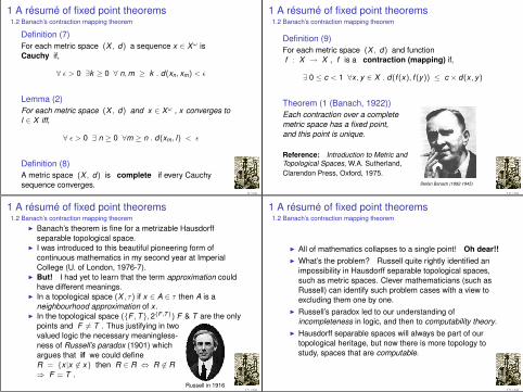
Definition (7)For each metric space (X , d) a sequence x ∈ Xω isCauchy if,

∀ ε > 0 ∃k ≥ 0 ∀ n,m ≥ k . d(xn, xm) < ε

Lemma (2)For each metric space (X , d) and x ∈ Xω , x converges tol ∈ X iff,

∀ ε > 0 ∃ n ≥ 0 ∀m ≥ n . d(xm, l) < ε

Definition (8)A metric space (X , d) is complete if every Cauchysequence converges.

9 / 59


Definition (9)For each metric space (X , d) and functionf : X → X , f is a contraction (mapping) if,

∃ 0 ≤ c < 1 ∀x , y ∈ X . d(f (x), f (y)) ≤ c × d(x , y)

Theorem (1 (Banach, 1922))Each contraction over a completemetric space has a fixed point,and this point is unique.

Reference: Introduction to Metric andTopological Spaces, W.A. Sutherland,Clarendon Press, Oxford, 1975.

Stefan Banach (1892-1945)

10 / 59


I Banach’s theorem is fine for a metrizable Hausdorffseparable topological space.

I I was introduced to this beautiful pioneering form ofcontinuous mathematics in my second year at ImperialCollege (U. of London, 1976-7).

I But! I had yet to learn that the term approximation couldhave different meanings.

I In a topological space (X , τ) if x ∈ A ∈ τ then A is aneighbourhood approximation of x .

I In the topological space (F ,T,2F ,T) F & T are the onlypoints and F 6= T . Thus justifying in twovalued logic the necessary meaningless-ness of Russell’s paradox (1901) whichargues that if we could defineR = x |x 6∈ x then R ∈ R ⇔ R 6∈ R⇒ F = T .

Russell in 191611 / 59


I All of mathematics collapses to a single point! Oh dear!!I What’s the problem? Russell quite rightly identified an

impossibility in Hausdorff separable topological spaces,such as metric spaces. Clever mathematicians (such asRussell) can identify such problem cases with a view toexcluding them one by one.

I Russell’s paradox led to our understanding ofincompleteness in logic, and then to computability theory.

I Hausdorff separable spaces will always be part of ourtopological heritage, but now there is more topology tostudy, spaces that are computable.

12 / 59

1 A résumé of fixed point theorems1.3 Tarski’s least fixed point theorem

I In any non-trivial logic (resp. any non-trivial programminglanguage) there will always be more truths (resp. possiblecomputations) than proofs (resp. programs).

I A proof (when consistently formed) approximates amathematical truth. For example, a 100% correct depiction ofAlan Turing can be approximated by an ascending sequence offinite grids of (i.e. proof) of so-called pixels as follows.

Neighbourhood approximationin a T2 space is correct.Approximation of truth bypixels is partially correct.How does a pixelapproximate truth?T0 separable spaces.

13 / 59


>

@@

@I

@@

@I

F

T

⊥> (pronounced top in lattice theory and both in four valued

logic) introduces the possibility of an overdeterminedmathematical value,

F ,T (pronounced false, true) typifies two well defined distinctvalues in a consistent Hausdorff separable mathematicaltheory,

⊥ (pronounced bottom in lattice theory and either in fourvalued logic) introduces the possibility of anunderdetermined mathematical value.

14 / 59


>

@@

@I

@@

@I

F

T

⊥We assume that information is partially ordered.⊥ @ F @ > and ⊥ @ T @ >.F 6v T and T 6v F (two valued logic is unchanged).x v y ⇒ f (x) v f (y) (functions are monotonic).

We envisage a vertical structure of informationprocessing orthogonal to a given horizontalmathematical structure.

15 / 59


Definition (10)A partially ordered set (poset) is a relation (X ,v ⊆ X × X )such that

x v x (reflexivity)x v y ∧ y v x ⇒ x = y (antisymmetry)x v y ∧ y v z ⇒ x v z (transitivity)

Definition (11)For each poset (X ,v) , (X ,@) is the relation such that,x @ y ⇔ x v y ∧ x 6= y .

Example (4)The real numbers (−∞,∞) are partially ordered by therelation x v y iff x ≥ y .

16 / 59


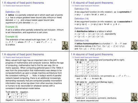
Definition (12)A lattice is a partially ordered set in which each pair of pointsx , y has a unique greatest lower bound (aka infinum or meet)denoted x u y , and unique lowest upper bound (akasupremum or join) denoted x t y .

Example (5)A set is a lattice when partially ordered by set inclusion. Infinumis set intersection, and supremum is set union.

Example (6)The extension of two valued truth logic from F ,T to⊥,F ,T ,> where F u T = > and F t T = ⊥is a lattice.

17 / 59


Definition (13)A two argument function (in infix notation) op is symmetric ifx op y = y op x for all x and y .

Definition (14)A two argument function (in infix notation) op is associative ifx op (y op z) = (x op y) op z for all x , y , & z .

Definition (15)A distributive lattice is a lattice in whichx t (y u z) = (x t y) u (x t z) , equivalentlyx u (y t z) = (x u y) t (x u z) .

Definition (16)A lattice homomorphism is a function f : X → Y overdistributive lattices X & Y s.t. f (x u y) = (f x) u (f y)and f (x t y) = (f x) t (f y) .

18 / 59


Many valued truth logic has an important role in the jointprogress of mathematics and computer science. Before the ageof computing, mathematics had to find its own way (for usmetric spaces). When computing gathered pace in the 1960s itwas from the presumption that mathematics was always to becomputed bottom-up upon a single machine architecture fromthe consistent nothing of ⊥ . Now, in today’s world of parallelnetwork based computing, there is an additional increasinglydemanding necessity that pre-computed possibly inconsistentinformation may arrive top-down from other sources (machineor human) to be reconciled (in whatever sense) with aconsistent mathematical model below.

Truth table for negation.P ⊥ F T >¬P ⊥ T F >

Negation is monotonic, distributive, and ¬¬P = P .19 / 59


Truth table for sequential and (computing left-to-right).P∧Q ⊥ F T >⊥ ⊥ F ⊥ ⊥F ⊥ F F FT ⊥ F T >> ⊥ F > >

Sequential and is monotonic, not symmetric as ⊥ ∧ F 6= F ∧ ⊥ ,and ⊥ ∧Q = ⊥ for each Q .

Truth table for parallel and (Belnap logic).P∧Q ⊥ F T >⊥ ⊥ F ⊥ FF F F F FT ⊥ F T >> F F > >

Parallel and is monotonic, symmetric, distributive,and above sequential and.

20 / 59


Definition (17)A poset is chain-complete if each chain x0 v x1 v . . . ∈ Xhas a least upper bound.

Theorem (2 (Tarski, 1955))Each monotonic function f : X → X over a chain-completeposet having a least member ⊥ has a fixed point. There existsa least fixed point having the property,

f (tn≥0 f n(⊥)) = tn≥0 f n(⊥)

Note: more general versions of this theorem exist forlattices. Historically the weaker poset version sufficedin early models for programming language design.

21 / 59


I Why? Tarski’s least fixed point theorem provided a simplecomputable model for loops of the 1960s. Wherecomputers were getting faster, demand for increasedrepetition was growing, yet scalability of programming wasstill manageable.

I Dana Scott provided a most influential topological modelfor the logic of computable functions using T0-separablespaces. A Scott topology (X , τ ⊆ 2X ) is related to thepartial ordering of a Scott domain by, if O ∈ τ , x v y , &x ∈ O then y ∈ O. A Scott topology (X , τ) is thusT0-separable. That is, if x @ y then there exists O ∈ τsuch that y ∈ O & x 6∈ O.

I T2 ⇒ T0 but T0 6⇒ T2 . So, how can the fixed pointtheorems of Banach and Tarski be reconciled?

22 / 59

1 A résumé of fixed point theorems1.4 Non-zero self-distance

Definition (18)A partial metric space (Matthews, 1992) is a tuple(X , p : X × X → [0,∞)) such that,

p(x , x) ≤ p(x , y) (small self-distance)p(x , x) = p(y , y) = p(x , y) ⇒ x = y (equality)p(x , y) = p(y , x) (symmetry)p(x , z) ≤ p(x , y) + p(y , z) − p(y , y) (triangularity)

Definition (19)An open ball Bε(a) = x ∈ A | p(x ,a) < ε .

Lemma (3)The open balls form the basis for a topology τp . This isasymmetric in the sense that there may be x , y suchthat y ∈ clx ∧ x 6∈ cly (i.e. T0 separation).

23 / 59


Definition (20)For each partial metric space (X , p) , (X , vp ⊆ X × X ) is therelation such that x vp y ⇔ p(x , x) = p(x , y) .

Lemma (4)(X , vp) is a partially ordered set.

Lemma (5)A metric space is precisely a partial metric space for whicheach self-distance is 0 . In such a space the partial ordering isequality.

Thus the notion of partial metric space is a generalisationof the notion of metric space through introducing non-zeroself-distance and motivated by the history of topology, logic,and computing.

24 / 59


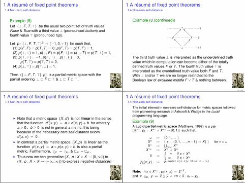
Example (8)Let ⊥,F ,T ,> be the usual two point set of truth valuesFalse & True with a third value ⊥ (pronounced bottom) andfourth value > (pronounced top).

Let p : ⊥,F ,T ,>2 → −1,0,+1 be such that,(1) p(F ,F ) = p(T ,T ) = 0, p(F ,T ) = p(T ,F ) = 1,(2) p(⊥,⊥) = 1, p(⊥,F ) = p(F ,⊥) = p(⊥,T ) = p(T ,⊥) = 1,(3) p(>,>) = −1, p(F ,>) = p(>,F ) = 0,

p(T ,>) = p(>,T ) = 0,(4) p(⊥,>) = p(>,⊥) = 1.

Then (⊥,F ,T ,>,p) is a partial metric space with thepartial ordering ⊥ @ F @ > & ⊥ @ T @ >.

25 / 59


Example (8 (continued))

>

@@I

F T

@@I

⊥

−1

0

+1

The third truth value ⊥ is interpreted as the underdefined truthvalue which in computation can become either of the totallydefined truth values F or T . The fourth truth value > isinterpreted as the overdefined truth value both F and T .With ⊥ and/or > we are no longer restricted to theBoolean law of excluded middle F ∨ T & nothing between.

26 / 59


I Note that a metric space (X ,d) is not linear in the sensethat the function d ′(x , y) = a× d(x , y) + b for arbitrarya > 0 , b ≥ 0 is not in general a metric; this beingbecause of the necessary zero self-distance axiomd(x , x) = 0 .

I In contrast a partial metric space (X ,p) is linear as thefunction p′(x , y) = a× p(x , y) + b is also a partialmetric. Furthermore, τp′ = τp , & vp′ = vp .

I Thus now we can generalise (X , p : X × X → [0,∞)) to(X , p : X × X → (−∞,∞)) to express negative distances.

27 / 59


The initial interest in non-zero self-distance for metric spaces followedfrom pioneering research of Ashcroft & Wadge in the Lucidprogramming language.

Example (9)A Lucid partial metric space (Matthews, 1992) is a pair(X ∗ω, pL : X ∗ω × X ∗ω → [0,1]) such that,

ω := 0,1, . . . X n := x : 0,1, . . . ,n − 1 → X ) for n ∈ ωX ∗ :=

⋃n∈ω X n

X ∗ω := X ∗ ∪ Xω

x :=

n if x ∈ X n

∞ if x ∈ Xω

pL(x , y) := 2−supn | n≤x, n≤y, ∀k<n . xk = yk

Note: ∀x ∈ X ∗ω . pL(x , x) = 2−x ,and x vpL y ⇔ x ≤ y ∧ ∀n < x . xn = yn .

28 / 59

1 A résumé of fixed point theorems1.5 A partial metric fixed point theorem

Definition (21 (Matthews, 1992))For each partial metric space (X ,p) , and for each x ∈ Xω ,x is a Cauchy sequence if,

∀ ε > 0 ∃ k ∈ ω ∀ n,m > k . p( xn , xm ) < ε

Definition (22 (Matthews, 1992))A partial metric space (X ,p) is complete if for each Cauchysequence x ∈ Xω there exists a ∈ X s.t.,

∃ limn→∞ p( xn , a ) = 0

29 / 59

1 A résumé of fixed point theorems1.5 A partial metric fixed point theorem

Definition (23 (Matthews, 1992))For each complete partial metric space (X ,p) a contractionmapping is a function f : X → X s.t.

∃0 ≤ c < 1 ∀x , y ∈ X . p(f (x), f (y)) ≤ c × p(x , y)

Theorem (3 (Matthews 1995))For each complete partial metric space (X ,p) having a leastmember ⊥, and for contraction mapping f : X → X there existsa ∈ X s.t. a = f (a) , p(a,a) = 0 , and a is unique.

Corollary (3a)This fixed point theorem for partial metric spaces generalisesBanach’s contraction mapping theorem (for metric spaces), andis a restriction of Tarski’s least fixed point theorem (for lattices).

30 / 59

1 A résumé of fixed point theorems1.6 A criticism of partial metric spaces

So, is there really any new maths here? Many Hausdorffseparable mathematicians might argue NO! as follows. Let,

Definition (24)A weighted metric space is a tuple(X , d , | · | : X → (−∞,∞)) such that (X , d) is a metricspace.Then, the argument goes, we can arrange the followingsupposed equivalence between partial metric spaces andweighted metric spaces.

31 / 59


Lemma (6)If (X , d , | · |) is a weighted metric space then

p(x , y) := d(x , y) +|x | + |y |

2

is a partial metric such that p(x , x) = |x | for each x ∈ X .

Conversely, if (X , p) is a partial metric space and

dp(x , y) := p(x , y)− p(x , x) + p(y , y)

2, |x |p := p(x , x)

then (X , dp, | · |p) is a weighted metric space.

32 / 59


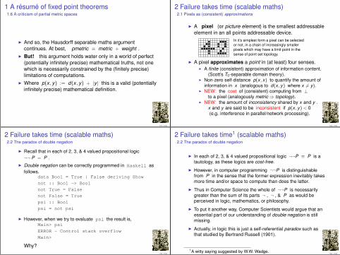
I And so, the Hausdorff separable maths argumentcontinues. At best, pmetric ≡ metric + weight .

I But! this argument holds water only in a world of perfect(potentially infinitely precise) mathematical truths, not onewhich is necessarily constrained by the (finitely precise)limitations of computations.

I Where p(x , y) := d(x , y) + |y | this is a valid (potentiallyinfinitely precise) mathematical definition.

33 / 59

2 Failure takes time (scalable maths)2.1 Pixels as (consistent) approximations

I A pixel (or picture element) is the smallest addressableelement in an all points addressable device.

sssssssssssss ssssssssssssss In it’s simplest form a pixel can be selectedor not, in a chain of increasingly smallerpixels which may have a limit point in thesense of point set topology.

I A pixel approximates a point in (at least) four senses.I A finite (consistent) approximation of information content.

(Scott’s T0-separable domain theory).I Non-zero self-distance p(x , x) to quantify the amount of

information in x (analogous to d(x , y) where x 6= y ).I NEW: the cost of (consistent) computing from ⊥

to a pixel (analogously metric⇒ topology).I NEW: the amount of inconsistency shared by x and y .

x and y are said to be inconsistent if p(x , y) < 0(e.g. interference in parallel/network processing).

34 / 59

2 Failure takes time (scalable maths)2.2 The paradox of double negation

I Recall that in each of 2, 3, & 4 valued propositional logic¬¬ P = P .

I Double negation can be correctly programmed in Haskell asfollows.

data Bool = True | False deriving Show

not :: Bool -> Bool

not True = False

not False = True

psi :: Bool

psi = not psi

I However, when we try to evaluate psi the result is,Main> psi

ERROR - Control stack overflow

Main>

Why?35 / 59

2 Failure takes time1 (scalable maths)2.2 The paradox of double negation

I In each of 2, 3, & 4 valued propositional logic ¬¬P ≡ P is atautology, as these logics are cost-free.

I However, in computer programming ¬¬P is distinguishablefrom P in the sense that the former expression inevitably takesmore time and/or space to compute than does the latter.

I Thus in Computer Science the whole of ¬¬P is necessarilygreater than the sum of its parts ¬ , ¬ , & P as would beperceived in logic, mathematics, or philosophy.

I To put it another way, Computer Scientists would argue that anessential part of our understanding of double negation is stillmissing.

I Actually, in logic this is just a self-referential paradox such asthat studied by Bertrand Russell (1901).

1A witty saying suggested by W.W. Wadge.36 / 59


Dana Scott’s inspired work has givenus the T0 topology to build cost-freemodels of partially defined information.But, computation can persist (perhapsindefinitely) without making any progress.Escher’s Waterfall lithograph tracesthe persistence of such a computationfull circle, as well as visualising it’smeaning as Tarski’s least fixed point ⊥ .

Equivalent to the paradoxof the Penrose Triangleimpossible object.

The supposed paradox disappearsin our intensional partial metricspaces where (dynamic) cost can becomposed with (static) data content.

WaterfallLithograph by M.C. Escher(1961)

37 / 59


I A partial metric space (X ,p) has been an interesting means toboth extend a metric space (X ,d) and quantify informationcontent for (static) partially defined data values.

I However, our study of double negation demonstrates that it musttake more (as in above some absolute minimum) time toevaluate ¬¬P than it does P .

I IDEA: Can we intensionalise partial metric spaces to modelnotions of cost observable at run-time (such as time)?

I Applying this idea to our earlier Haskell definitionpsi = not psi would mean that we could retain thetraditional Kleene, Tarski, & Scott domain theory meaningtn≥0 ¬n(⊥) of least fixed points and introduce cost as a meansto express such states as ERROR - Control stackoverflow .

38 / 59


Example (10)Let ⊥,F ,T ,> be the usual two point set of truth values False &True with a third value ⊥ (pronounced bottom) and fourth value >(pronounced top).

Let p : ω → (⊥,F ,T ,>2 → −1,0 ∪ 2−i |i ∈ ω) be such that,(1) pi (F ,F ) = pi (T ,T ) = 0, pi (F ,T ) = pi (T ,F ) = 2−i ,(2) pi (⊥,⊥) = 2−i , pi (⊥,F ) = pi (F ,⊥) = pi (⊥,T ) = pi (T ,⊥) = 2−i ,(3) pi (>,>) = −1, pi (F ,>) = pi (>,F ) = 0, pi (T ,>) = pi (>,T ) = 0,(4) pi (⊥,>) = pi (>,⊥) = 2−i .

Then each (⊥,F ,T ,>,pi ) is a partial metric space with thepartial ordering @i⊆ 2−i ,0,−12 s.t. ⊥ @i F @i > & ⊥ @i T @i >.

The intension is that pi (⊥,⊥) expresses the time taken inevaluating a totally defined value F or T .

39 / 59


Example (10 (continued))

>

@@I

F T

@@I

⊥

AAAAAK

⊥

pi (>,>) = −1

pi (F ,F ) = pi (T ,T ) = 0

pi (⊥,⊥) = 2−i

p0(⊥,⊥) = 2−0

And so, suppose we wish to define the whole meaning of ¬¬P forP in some given intension i . Assume also (for simplicity) eachoperation in our intensional logic takes one unit of time to evaluate.Then, pi (¬¬P,¬¬P) = pi (P,P)× 2−2 . We now havepi (P,P) > pi (¬¬P,¬¬P) and ¬¬P = P . We now have amathematical model for Escher’s Waterfall.

40 / 59

2 Failure takes time (scalable maths)2.3 Wadge’s hiaton

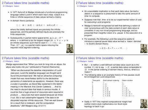
I In 1977 Ashcroft & Wadge introduced a functional programminglanguage called Lucid in which each input (resp. output) is afinite or infinite sequence of data values termed a history.

I In domain theory parlance,

〈〉 @ 〈a〉 @ 〈a,b〉 @ 〈a,b, c〉 @ 〈a,b, c,d〉 @ . . .

where the totally defined inputs are precisely the infinitesequences, and the partially defined inputs are precisely thefinite sequences.

I Subsequently in partial metric space terms pL(x , y) = 2−n

where n is defined to be the largest integer (or ∞ if x = y isan infinite sequence) such that for each 0 ≤ i < n xi = yi .Then (X ∗ω,pL) is a partial metric space inducing therequired initial segment ordering.

41 / 59


I An unavoidable implication is that each data value (termed adaton) in a sequence is presumed to take the same amount oftime to compute.

I Suppose now that time is to be our experimental notion of costfor executing Lucid programs.

I Wadge & Ashcroft recognised full well that defining a notion ofcost synonymous with the data content of each data value isunrealistic in any non trivial programming language, and sopresented their insightful vision of a pause in the execution of aprogram.

I For example, the following Lucid-like sequence seeks tointroduce a special pause data value termed a hiaton denoted∗ to Scott’s domain theory.

〈∗,2,3, ∗,5, ∗,7, ∗, ∗, ∗,11, . . . 〉

42 / 59


Wadge appreciated that "When you look for long into an abyss, theabyss also looks into you" (attributed to Friedrich Nietzsche).

"When we discovered the dataflow interpretation of Lucid(see post, Lucid the dataflow language) we thought we’dfound the promised land. We had an attractive computingmodel that was nevertheless faithful to the declarativesemantics of statements-as-equations. However, there wasa snake in paradise, as David May explained in the fatefulmeeting in the Warwick Arts Center Cafeteria. ... And it’sthe need to discard data that leads to serious trouble. Itcould be that a huge amount of resources were required toproduce ..., resources that were wasted because we threwit out. But a real catastrophe happens if the data to bediscarded requires infinite resources. Then we wait foreverfor a result that is irrelevant, and the computationdeadlocks." (Bill Wadge’s blog, 6/12/11)

43 / 59


I But ∗ is neither a well defined null data value (such as is thenumber 0 ) nor is say 〈∗,2〉 a partial data value comparable to〈2〉 in the partial ordering of domain theory. And so, what is ahiaton ?

I The following table is an example history of how pauses couldbe envisaged as Lucid sequences.

Time point Scott domain ordering Hiaton intuition0 〈〉〈〉1 v 〈1〉〈1〉2 v 〈1〉〈1, ∗〉3 v 〈1, 2〉〈1, ∗, 2〉4 v 〈1, 2〉〈1, ∗, 2, ∗〉5 v 〈1, 2, 3〉〈1, ∗, 2, ∗, 3〉6 v 〈1, 2, 3〉〈1, ∗, 2, ∗, 3, ∗〉7 v 〈1, 2, 3〉〈1, ∗, 2, ∗, 3, ∗, ∗〉. . . . . . . . . . . .

I Sadly in 1977 this inspired computational insight hadneither metric-style mathematics nor Scott-styletopology to back it up!

44 / 59


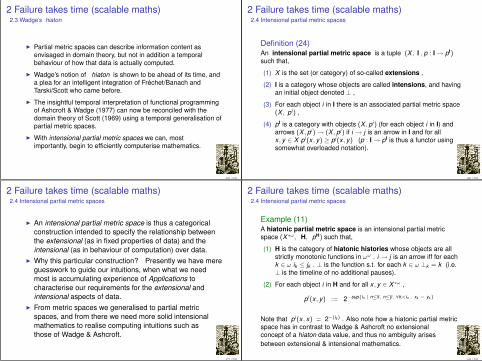
I Partial metric spaces can describe information content asenvisaged in domain theory, but not in addition a temporalbehaviour of how that data is actually computed.

I Wadge’s notion of hiaton is shown to be ahead of its time, anda plea for an intelligent integration of Fréchet/Banach andTarski/Scott who came before.

I The insightful temporal interpretation of functional programmingof Ashcroft & Wadge (1977) can now be reconciled with thedomain theory of Scott (1969) using a temporal generalisation ofpartial metric spaces.

I With intensional partial metric spaces we can, mostimportantly, begin to efficiently computerise mathematics.

45 / 59

2 Failure takes time (scalable maths)2.4 Intensional partial metric spaces

Definition (24)An intensional partial metric space is a tuple (X , I ,p : I→ pI)such that,

(1) X is the set (or category) of so-called extensions ,

(2) I is a category whose objects are called intensions, and havingan initial object denoted ⊥ ,

(3) For each object i in I there is an associated partial metric space(X , pi ) ,

(4) pI is a category with objects (X ,pi ) (for each object i in I) andarrows (X ,pi )→ (X ,pj ) if i → j is an arrow in I and for allx , y ∈ X pi (x , y) ≥ pj (x , y) (p : I→ pI is thus a functor usingsomewhat overloaded notation).

46 / 59


I An intensional partial metric space is thus a categoricalconstruction intended to specify the relationship betweenthe extensional (as in fixed properties of data) and theintensional (as in behaviour of computation) over data.

I Why this particular construction? Presently we have mereguesswork to guide our intuitions, when what we needmost is accumulating experience of Applications tocharacterise our requirements for the extensional andintensional aspects of data.

I From metric spaces we generalised to partial metricspaces, and from there we need more solid intensionalmathematics to realise computing intuitions such asthose of Wadge & Ashcroft.

47 / 59


Example (11)A hiatonic partial metric space is an intensional partial metricspace (X ∗ω, H, pH) such that,

(1) H is the category of hiatonic histories whose objects are allstrictly monotonic functions in ωω . i → j is an arrow iff for eachk ∈ ω ik ≤ jk . ⊥ is the function s.t. for each k ∈ ω ⊥k = k (i.e.⊥ is the timeline of no additional pauses).

(2) For each object i in H and for all x , y ∈ X ∗ω ,

pi (x , y) := 2−supin | n≤x, n≤y, ∀k<in . xk = yk

Note that pi (x , x) = 2−(ix ) . Also note how a hiatonic partial metricspace has in contrast to Wadge & Ashcroft no extensionalconcept of a hiaton data value, and thus no ambiguity arisesbetween extensional & intensional mathematics.

48 / 59


The story so far ?I With Lucid Wadge & Ashcroft made great progress to

reconcile Scott’s T0 separable domain theory withprogramming language design & implementation.

I Partial metric spaces brought metric spaces into thisresearch.

I Hiatonic partial metric spaces provide more evidence thatthere exists a happy partnership between topology (T2 &T0), programming language design & implementation, andquantitative necessities of contemporary computing.

I Where now? from the property pi(x , x) = 2−(ix ) of ahiatonic partial metric space (X ,H,pH) & i ∈ H we can inferthat it is not possible in general to determine each ofthe amount of data content in x and the number oftime delays in x .

49 / 59


We could redefine a hiatonic partial metric space as follows inorder that the information content & time delays (moregenerally cost) can each be recovered.

Example (12)A costed hiatonic partial metric space is an intensionalpartial metric space (X ∗ω,H,pH) such that suppose ndenotes x u y for some x , y ∈ X ∗ω . Then,

pi(x , y) := 2−n+(1−2−in )

Here in is to be read as the total number of additional delaysso far in producing the n′th daton (x u y)n in intension i .

50 / 59


I A costed hiatonic partial metric space improves upon ahiatonic partial metric space in the sense that pi(x , x) is asingle number from which can be uniquely determined theamount of data content (namely 2−x ) and a cost forcomputing x ( namely 2−1+2−in ) .

I However, our construction (so far) highlights a significantweakness in that pi is only modulo any one givenintension i . At so-called run-time in a computation a delaymay arise as a result of behaviour that could not have beenpredetermined. In such a situation we would require anarrow construction i → j and dynamic intensional partialmetric space (X , pi→j) such that,

i → j ⇒ ∀ x , y ∈ X . pi(x , y) → pj(x , y)

51 / 59


Bill Wadge

I Wadge is much respected for his PhDUC Berkeley research known as theWadge hierarchy, levels of complexityfor sets of reals in descriptive set theory.

I Wadge’s later insight that a complete object is "one that cannotbe further completed" led from metric spaces (of completeobjects), to Lucid (for programming over metric spaces), topartial metric spaces (domain theory for metric spaces), andnow to cost to reconcile partial metric spaces with (say)complexity of algorithms.

I "I don’t know if infinitesimal logic is the best idea I’ve ever had,but it’s definitely the best name. So here’s the idea: amultivalued logic in which there are truth values that are notnearly as true as ’standard’ truth, and others that are notnearly as false as ’standard’ falsity"(Bill Wadge’s blog, 3/2/11).

52 / 59

2 Failure takes time (scalable maths)2.5 Conclusions and further work

I In a demand driven (as opposed to data driven) programminglanguage some potential catastrophes are never encountered.But, for the usual decidability reasons in computation andincompleteness of logic, not all catastrophes can be so avoided.

I Our monotonic treatment of failure takes time may thus bepartially correct in the sense of domain theory, but is it still tooweak to be useable in practice?

I A sequence p0,p1, . . . of consistent partial metrics as justdescribed is an interesting step forward, but hardly a computablenotion of partial metric. That is, is there a notion of partial metricthat can express the best and worst of computation?

53 / 59


While time is a useful starting point for working bottom up toward anotion of cost, we also want to ask from what properties can beidentified to work down?

Cost is observable. Our first foundational assumption forcost is that it is a logic of observable properties (in the sense ofa traditional process calculus.

Cost is monotonic. Our second foundational assumption forcost is that it always increases with respect to whatever may beour chosen cost axis, usually time or space.

pc(x , y) > pc+1(x , y)

Note: terms such as c + 1 presume a suitable predefinedalgebra/logic of cost .

54 / 59


Cost is realistic. Our third foundational assumption for cost is thatany given mathematical/logical model of computational cost that iswholly a static theory cannot be extended beyond it’s own limits. Incontrast real-world computing is dynamic, showing no signs yet ofreaching whatever may prove to be it’s ultimate limits and impactupon society. Our research continues to thrive upon the assertion thatwe refute an either all static or all dynamic approach, but rathervoluntarily subject ourselves to building a balanced discipline of static& dynamic mathematics/logic for future use.

55 / 59


I Conclusions: metric spaces and topology are excellent for aformer age of strong mathematics where cost could beignored.

I Now we live in an age where the cost of globalisation is intrinsicto our very survival, calling for compassion back to the worldwe once ignored.

I I find the history of metric spaces,topology, logic, incompleteness,computer science, and partial metricspaces to be a fascinating personaljourney of discovery, inclusion,compassion, and cost in ourcompetitive world.

c© Buddha of Compassion Society

56 / 59


I Further work: there has been an unfortunatecultural divide in Computer Scienceseparating mathematical models & logicfrom the more successful complexity ofalgorithms, now known as discrete maths.

I A pronounced winner takes all mentalityreminiscent of tragic divides in east meetswest Holy Wars pervades today’s IT Wars.

I The history of Hagia Sophia (Holy Wisdom)from church, to mosque, to secular museuminspires our mathematical research to be aformalism of disparate unity for our world.

I We hope to have a local workshop at ComputerScience Warwick within the year on the themeof Scalable Partial Topology.

Hagia Sophia, Istanbul

57 / 59


"It has long been my personal view that theseparation of practical and theoretical workis artificial and injurious. Much of thepractical work done in computing, both insoftware and in hardware design, is unsoundand clumsy because the people who do ithave not any clear understanding of thefundamental design principles of their work.Most of the abstract mathematical andtheoretical work is sterile because it hasno point of contact with real computing.One of the central aims of the ProgrammingResearch Group as a teaching and researchgroup has been to set up an atmosphere inwhich this separation cannot happen."

Christopher Strachey (1916-75)Founder of the Oxford ProgrammingResearch Group (1965)

S c a l a b l e P a r t i a l T o p o l o g y

58 / 59


elbalacS

P a r t i a lTopology

Failure takes time !!!

Waterfall

59 / 59

1 a résumé of xed point theorems - dcs.warwick.ac.uksgm/a7-2x2.pdf · 1 a résumé of xed point...

Documents