1 11~~iiiii~llll! lijliil~li~lll~~mlflll llllllll...
TRANSCRIPT

-1 11~~ IIIII~ llll llijliil~li~lll~~mlflll llllllll ~lill~ 1 shyo 1160 0072930 5 TRI- PPmiddot-95- 2 I INTRODUCTION Jan 1995
Magnetic trapping of spin-polarized neutral atoms and its limits
V E Shapiro
TRIUMF 4004 Wesbrook Mall Vancouver BC Canada V6T 2AFERMlLA MAR
Abstract
I We investigated the limits of magnetic methods of trapping neutral atoms in
a spot of small size and small polarization misalignment The analysis covmiddot
ers various methods of trapping with static and rotating magnetic field In
particular new rotating field methods having advantages are proposed They
differ from the recently invented top type by employing a slow rotating
field resonant to the orbiting atoms rather than much faster rotation Also
a theory of the top trap is developed It elucidates important features of trapmiddot
ping lying beyond the timemiddot averaged potential concept General criteria on
the trapping temperature as a function of size and misalignment parameters
are established for various methods
(Submitted to Physical Review A)
PACS numbers 3280Pj 8570Nk 4250Vk
The method of neutral atom trapping by magnetic fields has been successfully demonshystrated since 1985 [1-31 and its usage and development is in rapid progress (see eg Refs [4 -71) Many questions have arisen and there are many factors to consider if requirements on the smallness of atom spot and polarization misalignment are imposed First of all the question abuut the most appropriate magnetic field configuration is very important since the magnetic potential well is shallow and able to trap only atoms of rather low temperatures - 10- 3 K Even deeper cooling of the atoms is required if low polarization misalignment is critical
Addressing the problem we derive simple criteria and present scales and estimates allowshying one to judge and compare various types of magnetostatic traps We consider the static field traps and the type with rotating field (top trap) recently invented by Cornell [71 and investigated very sketchily in the literature The top trap is considered in more detail and its new features are elucidated We also draw attention to trapping methods with rotating lields of much lower frequency than the top type These methods are discussed for the lirst time Our earlier results reported to the TRIUMF TRINAT group and summarized ill [81 are partly included in the present consideration
II MAIN ASSUMPTIONS AND DEFINITIONS
The wellmiddot known principle behind a magnetic trap is that magnetic dipoles may be trapped by a lucal field minimum (local maxima are forbidden) and that the atoms prepared in select Zeeman levels with the resultant (average) magnetic moment I- antiparallel to an applied magnetic field B fullow adiabatically the magnetic field lines across the volume of the trap In such states the atoms are attracted to a point of minimum of the force potential
U(r) = -I-B(r) + Mgz = pB(r) + Mgz (I)
with H = IBI and p = 11-1 = const gt 0 ie to a minimum of the magnetic field magnitude (here M is the atomic mass 9 the gravity acceleration) The model can be applied to the case of sluw time-varying fields in which the frequency spectrum of B(t) = B(r(t)t) for a trapped atom is in a range well below the Zeeman frequency in the field This is what une means by a magnetostatic trap The trapped atoms are vulnerable to background gas cullision~ and the mean free time between collisions should exceed the desired trapping time
We will first consider static field traps At the trap centre
oB My-=-- (2)Oz p
Also the curvature of the field B at the trap centre should be positive to provide confinement in three urthogunal directions The curvature is given by the matrix iP UOriork In the coordinate frame where the matrix is diagonal the natural frequencies of small amplitude atomic uscillation are given by
Wi = JJl olB (3)M urf
2
We will assume that the directions ri coincide with the coordinate frame xyz and the point r = degwill be taken at the trap centre
The lower edge of the potential weU of U(r) Eq (I) is located where Eq (2) is again satisfied after the field curvature changes sign The upper edge may be at infinity or where the field goes through a maximum again satisfying equation (2) One more edge leading to the leakage of particles is in the vicinity of B = degwhere the adiabaticity is violated What one usually needs is for the well to be as deep as possible within a given atom spot size rather than a deep well with a wider but flat bottom Requirements on the uniformity of atom polarization alignment within the atom spot reinforce this point In particular the hole centered at B = degshould not be inside the atom spot and neither should the field curvature vary considerably inside
In the case of a small atom spot its average spatial scales r are related to the trapping temperatures Ti by
kTi = Mrl(O) = 2Mw~r (4)
We define the trapping temperature such that kT2 is the total initial kinetic energy of the atoms divided by the number of atoms loaded into the trap centre The conditions correspond to the loading from an optical trap having much better confinement The energy of oscillation is distributed equally in average between the kinetic and potential energy and this results in the factor 2 in Eq (4) The definition does not depend on interactions between atoms and whether thermalization takes place Obviously the requirements on preliminary cooling of the trapped atoms are directly related to the trapping temperatures specifically their upper bounds for given spot sizes and polarization misalignment Our goal will be to determine such bounds
The accuracy of Eq (4) can be judged by the frequency shift OWi Wi caused by anharshymonicity For small=1 lampiilwi = if 1
roughly where 1 is a characteristic scale of field curvature variation For typical trapping geometries I is about three times smaller than R the radius of the main magnetic coil so for amplitudes not larger than ~ OIR we may rely on Eq (4) In fact the atom spot sizes of interest are within this scale
The static field traps of interest employ the field B(O) aligned vertically and as a meashysure of deviation of atomic polarization from z-alignment within the spot we will take the quantity
P = l-IJ(r)IJ = I -IBz(r)B(r)1
which in the case of small atom spots reduces to
p=~1 L ~~Bzl (5)2 r=rVz ar B
where the derivatives are taken at r = 0 Proceeding from these notions and definitions we will consider first in Sees II-V the
static field traps The rotating field traps require a modified approach which is undertaken in Secs VI and VII
III THE AXIAL SYMMETRY TRAP
The magnetic coil configuration we address here is a set of concentric coils of arbilrary radii and currents with the axis in the z direction Simple examples are the opposing coils
3
and spherical hexapole traps (Fig I(abraquo Obviously the arrangements with B(O) = 0 eg the spherical quadrupole of such currents that 8B8z at the quadrupole centre satisfies Eq (2) do not do for the traps of interest The analysis below makes this and other requirements clear and puts them on a quantitative basis The quadrupole configuration is merely one of the axial symmetry traps Coils with parallel currents rather than opposing is an example of different trap configuration
The magnetic field components near the axis can be presented up to second order in r 1 by the well-known general expansion
B(zr1) = Bo(z) - ~ B~(z)rI
Br(zr1) = -~ B(z)x Bv(zrd = -~ B~(z)y
where ri = xl +yl Bo(z) is the magnetic field at the axis of symmetry B(z) = dBo(z)dz and B~(z) = ~Bo(z)dzl These quantities at the trap centre are related through Eqs (2) and (3) yielding
BoB~ Mg IBol =--shy
W~ = pound B~BoMI8I
1 1 J B - 2B~Bo Wr = Wv = M 41 Bol
As a consequence
B~l gt 2BoB gt 0 B = (MgJ)l (6)
Evaluating P of Eq (5) and relating ri to the perpendicular temperature T1 = (Tr +Tv)2 via definition (4) one obtains
Bl l kTl ( w )P = 8B~ r1 = 2JIBol 1+ 2w~
Excluding Bo (using the latter relation) results in
kT1 r wl
~ = CIVP where CI = __r (7)M9V r i2 w +w~2
This relation allows one to determine the trapping temperature required to provide a given (slllall) alom spot size and misalignment Its upper bound is given by
11 = ~9 JP r i2~ 04 x 10-4 K (8)
4
Ilere (and further on) the numerical estimates are for M = 40 amu We assume ill Eq (8)
that f = 05 cm and P = 005
We may also interpret the relations (7) and (8) as a bound on the product Pri for a given trapping temperature TJ
~ kTJ kTJ VPrj2 = -M lt -M (9)
gCI 9
Similarly the product pz1 can be presented in the form
fiii = k~w +w~2 lt k~ (10)Mg wzw Mg
where however TJ is bounded by Eqs (7) and (8) No dependence on the magnetic field appears and only one atomic parameter the atomic
mass enters Eq (8) as well as the r hs of Eqs (9) and (10) Originally we came to this result by a different approach [8J Thus whatever the set of concentric coils their radii and currents are the relation (7) and its consequence Eqs (8) (9) and (10) i~ true With this the derivation implies that the magnetic field provides trapping and the atom spot is small compared with the spatial scales of oscillation anharmonicity of atoms in the trap
The formulas (7) middot ( 10) seem in evident contradiction with the case 9 = O But in that case B~ = 0 and the requirement (6) cannot be satisfied ie a trap of axial symmetry with the desired properties cannot be realized
The larger the atomic mass M the higher the temperature that can be used for trapping In principle the derivation is applicable to a macroscopic particle provided its state with p antiparallel to Band IJ = const has a sufficient lifemiddot time Note that the bound Eq (8) written in terms of mean square velocity rather than temperature is a universal function entirely independent of free parameters
1v = 3gPri2
which for P = 005 and r = 05 cm results in r ~ 15 cmsec
IV THE COIL + CURRENT BAR TRAP
The magnetic field coil configuration considered here has vertical current bars which generate a quadrupole field in the horizontal plane (Fig 2(a)) The vertical field is formed mainly by the current of a round coil so that to second order in coordinates
B = Bo(z) - ~B~(z)r~
Bz = -GB~(z) +Q )x ( II)
Bv = - GB~( z) - Q) Y
where (Qx -Qy) are the components of the quadrupole field and Bo(z) is the axial field of the round coil For a thin coil of radius R placed at z = - D
5
Bo(z) = ( D1 + Rl )31 (D +z)l + Rl Bo
with Bo = 0(0) determined via the condition Eq (2) As a result
L = D D1 + R1w1 - 9 where ( 12)- L 4D1 - R1
and in view of Eq (4) we obtain the relation
kT 2(] ( 13)Mg(] = -L-
Obviously the area of interest and applicability of Eq (13) is where v7i is small compared
with L One may use Eq (13) where Eq (4) can be used (ie where vii - OlD or smaller) The spatial ~cale L is bounded by the fact that D gt R2 and that the coil radius R cannot in practice be made arbitrarily small For a given R the minimum of L is ~ R3 for Dl Rl = 2( 65 - 7) ~ 2 Thus the relation (13) imposes by itself without any additional restriction 011 polarization misalignment a strong bound on the trapping temperature For
R = 1J = 5 cm and the spot size v7i = 05 cm the bound equals
Mg 3ii 4 T = T D - 07 x 10- K
Requirements for small polarization misalignment impose upper bounds on the trapping temperatures Tz Ty rather than T Evaluating p of Eq (5) for an atom spot of temperature 1 = 7~ = 11 we obtain
1 1P = kTJ w w
where c1=1+~+~21J Bo(1 4wz 4wv
With Bo determined via Eq (2) this results in the following bound
Mg2L I 4TJ = --P-08 x 10- K (14)
k C1
where
4D1 - R1 L = L 3D1
and the numerical example is for R = D = 5 cm C1 = 2 and P = 005 It is worth noting that the prod uct Pii is gi ven by the formula similar to (10)
p-i = kJTTJ ~~ Mg V4 4D1 - R1
where 1 and T1 are bounded by Eqs (13) and (14) Agaill as for the axial symmetry traps the upper bounds on the trapping temperatures
do 1I0t dcpml 011 the magnetic field magnitude and only one atomic parameter the mass M cntcrs the criteria for 1~ and fl
6
V THE BASEBALL AND OTHER STATIC FIELD TRAPS
The baseball geometry consists of a loop of wire wound similar to the seams of a baseball (Fig 2(b)) and an axial pair of anti-Helmholtz coils to generate the required axial field to compensate gravity at the baseball centre The baseball loop current produces no field gradient at the centre just field and field curvature and so this point i~ the centre of the trap The anti-Helmholtz coils generate no field or curvature and thus the curvature is decoupled from the gradient unlike previously discussed configurations
The field expansion near the trap centre is given to second order in coordinates by the functional form Eq (II) whereas before IB~I = MgJ while Bo B~ and Q are determined by the baseball coil radius R and current I by
Bo = 21 5R
B = 2Bo o R1
Q = 5Bo 2R (15 )
The natural frequencies Wi (Eq (3)) take the form
l=JB w M 0
(Qplusmn Mi)l1=J 1~
wt M Bo 1_w
2 (16)
where Wplusmn = Wr~ and Bo and B~ are assumed (without loss of generality) positive At Bo ~ 2MgR3R the dimension y becomes untrapped In the limit of large Bo and hence large Q the frequencies Wplusmn become equal and three times larger than w bull
From (4) (15) and (16) follows the relation
2f1 B o Zl 27 x IO-~ K T = -A- R1 ( 17)
The numerical estimate is for R = 5 cm fit = 05 cm fI = fiB the Bohr magneton and Bo = 101 gauss Such a baseball field is generated by the current I = 5BoR2 = 1250 ampere-turns To increase it by much creates technical problems so the cited figure of T seems a characteristic scale for the baseball traps
Now let us investigate the polarization characteristic of Eq (5) For the baseball trap we obtain
p = 4f1k [Tz (I + ~~J +T~ (I + ~~~) ] ( 18)Bo
It follows that the upper temperature bound is given by
0TJ = 2f1 p 7 x IO-~ K
where the numerical example is the same as in Eq (17) with P = 005 Since the cited horizontal temperature bound is 25 times larger than the corresponding vertical temperature bound in (17) the level of polarization misalignment for the given vertical size spot and isotropic trapping temperature is much better than for P = 005
Finally we note that the baseball trap and the traps employing a bias field Bo and axial confinement from a set of concentric coils and transverse confinement from a four-wire quadrupole field have much in common in particular the relations (II) (16) and (18) are the same An example is the loffe trap which has two concentric coils with equal currents (Fig2(c)) As seen from Eqs (16) and (18) the bias field should be within certain limits to provide both small spot size and polarization misalignment and therefore though more freedom in the parameters of Bo and Wi appear the upper temperature bounds cannot change mudl compared with the case of the baseball trap
7
VI THE TOP TRAP
The top (time-averaged orbiting potential) trap is a recent invention [7] It employs a combination of static and rotating magnetic fields
B(rt) = Boc(r) + b(t) ( 19)
where Boc is an axial quadrupole field generated by uopposing coils with the axis in the vertical direction (Fig I(a)) and b is a large-amplitude uniform field quickly rotating in the horizontal plane ULarge and quickly are in the sense
b1 raquo B~ Wi ct n lt nz (20)
where Bo = Bo(O) is the vertical field at the trap centre n is the frequency of rotation of the field b nz the Zeeman splitting in the field and Wi with i = x y z are the natural frequencies of small amplitude smoothed vibration The inequality n lt nz makes the principle behind the top trap the same as for a static field trap The atomic magnetic moment adiabatically follows the field rotation which in view of b1 raquo B~ rotates almost in the horizontal plane The top trap has a rather small atom spot This and the rotation of the atomic polarization are attractive features for experiments on polarized neutral atoms
Now unlike the static field traps the potential U( r) Eq (I) varies periodically in time That the oscillating component of magnetic force is large and influences the confinement critically makes the analysis of confinement more complex than that of a static field trap The atom motion r(t) is a superposition of a high frequency small radius orbit and a smoothed oscillation in the averaged potential characterized by low frequencies Wi laquo n The standard asymptotic method of nonlinear mechanics can be applied to the analysis and we used it at first However the conventional second order perturbation theory results in losing ~ight of interesting features elucidated below We obtained them by a different method employing the coordinate frame rotating with the field This greatly simplifies the analysis and its correctness becomes eiL~y to check because the confinement is then governed by the time-independent potential
U(R) = flB(R) - ~Mn1(X1 + y1) + Mgz (21 )
with B(R) = B(rt) R = (X yz) and the second term in the rhs representing the centrifugal forces Assuming the static field configuration an axial quadrupole the total field B(R) components read
IBx = b-middot BX
By = --BY
= (22)
0 0 B Bo + Bz2 2
The coordinates X Yare expressed via x y by
(X Y) = (x cos(Ot) + y sin(nt) -x sin(nt) + y cos(nt))
if t = 0 is taken as a moment where b is directed along x Neglecting other influences the atomic motion equation takes the form
il = _ I auMaR - 2(n x RImiddot (23)
8
The second term in the Lhs is the Coriolis force and = (00 fI) The equilibrium point R = Ro of Eq (23) determined by aufaR = 0 corresponds to the synchronous rotation of trapped atoms about axis z at frequency fl Taking R = 0 for the center of rotation we obtain Ro = (XoOO) where Xo is determined from
2b 2w~(Xo) (24)Xo = - B~ fll - 2w~(Xo)
with
l Jl Bl Wo = 8M iJ and 1J = B(Ro)
The frequency Wo characterizes the transverse oscillation r(t) in the potential U(r t) avshyeraged over explicit t dependence The regime of fast rotation implies Wo laquo fI and hCllce B~Xo laquob Because of that and in view of Bo laquob it follows B(Ro) band wo(Xo) wo(O)
The equation aU(R)az =0 takes the form
B = _ Mg B (25) o Jl Bo
and represents the balance condition between the gravitational and magnetic forces It differs from that of the static field traps Eq (2) considerably since B raquo Bo and it is no harm for the top trap to have Bo arbitrary smal While for the static traps B~ is fixed by atomic parameters the B~ of Eq (25) is not This equation may be viewed as a relation betweell B~ band Bo The larger B~ is the larger the confinement spring w~ which bchaves like B~2B (MgJl)2bBo
Let us consider small oscillation near the state R = Ro Linearizing Eq (23) we arrive at the system of three coupled oscillators
x+ (26 l - fll)(X - Xo) = 2f1Y - 4woLlz
y + (2w~ - fll)y = -2f1X (26)
Z +8(w~ - 62)z = -4woLl(X - Xo)
llere we denote by 6 the small frequency parameter
6 = wo~ol laquowoB
and 6 = (I - B~Xo2b)6 6 The partial frequency of z oscillation w = j8(w - 62)
differs considerably from the natural frequencies fIplusmn (given further by Eq (27)) of coupled transverse oscillation Because of that and since Ll is small the coupling between the vertical and transverse oscillation is a tiny effed We will neglect it for simplicity On the contrary the coupling between the X and Y oscillations is strong and should be taken into account middot bull i dly The lImiddotpu l - springs of partial X and Y osdllators of Eq (26) are difrerent alld this is of imporl c resulting in a specific gyroscopic 1Il00Iulation of free oscillation as elucidated below
Evaluating from Eq (26) the natural frequencies of transverse oscillation we obtain
fI~ = fl2 +w plusmn j4f12W +w~ (27)
9
whcre
wl =w~plusmn62
The regime of small oscillation is stable unless fll lt 2w~ (more about this condition is in Sec VII) In view of fll raquo w~ the transverse oscillation reduces approximately to a simple form which after returning to the fixed coordinate frame is given by the complex fundion p(t) r(t) t iy(t)
p(t) Xoeill + (X+eitl +X_e- il)ei61 (28)
So r i(t) = Ip(t)1 x(t) = Re[p(t)J and y(t) = Im[p(t)J Here Xo is given by Eq (24) Xplusmn are complex constants determined by initial conditions fI and fIplusmn assumed (without loss of generality) positive and
w = fI+ - fI_2 ~Wo
6 = fI _ fI+ + fI_ w4
(29)2 803
As seen from Eq (28) the normal transverse oscillations in the fixed coordinate frame are of different frequencies w + 6 and W - 6 rather than of equal frequency [7J The oscillashytions of different frequencies rotate in opposite diredions This results in the polarization of harmonic oscillation of frequency w rotating slowly at frequency 6 in the direction of the rotating magnetic field This modulation which we call gyroscopic can be 100 deshypending on the conditions of loading and manifests itself when the time of observation is commcnsurate or larger than 16 The effect cannot be explained by the time-averaged potential concept and described in its terms That concept results in a picture of degenerate transverse oscillation governed by averaged potential-like forces It loses sight of gyroscopic forces induced by high frequency forces
Another important feature we found is that the loading of atoms into the center r = 0 and with zero velocity does not eliminate the free oscillation and makes its amplitude larger than Xo by more than fIw times
p(t) = p(ol(t)
Xo einl= _ [ifl 6 sin(wt) +cos(wt)] eih (30)
The physics is easy to understand noticing that the velocity oscillations p( I) of high and low frequency motion havc nearly equal amplitudes
For the case of nonzero initial conditions
p(l) = p(ol(t) + plaquo)(l)
with
plaquo)(l) = [p(O) -wiP(0)6 sin(wl) + p(O) cos(wt)]ei61 (31 )
where p(O) = x(O) + iy(O) alld p(O) = x(O) + iY(O) Provided Ip(O) is of the same order or smaller thau Ip(O)w ic for loading dose to the cellter of the trap the two types of
10
motion pta) ilnd p(e) become of same amplitude when the initial kinetic energy is about MOl X In terms of temperature Tl of trapped atoms this corresponds to Tl ~ Tio) where
l T(o) = MOl Xl = 2Jlb w ~ 14 X 10-6 K (32)l k deg k Ol
The numerical estimate is for the example b = 10 G Jl = JlB and wO = 10- 1 For the
cited data atomic mass M = 40 amu and static field gradient B~ = 10l Gcm we obtain roughly Bob = 007 w27r = 21 Hz and 16 = 06 s With this Xo = 004 mm and Ip(o)(t)1 ~ 04 mm
So for the atoms loaded into the center of trap at a temperature Tl small compared with Tio) the transverse size of the atomic spot is about r l = Ip(o) I which is independent of Tl and given by the formulas and estimates above In the opposite case when Tl P 1~
approximately (for Ip(O) raquo wlp(O)1)
- kTlri = -- (33)Mwl
The bar here and below means the average over the initial conditions and per period 271 w The dependence on the motion of low frequency 6 is retained but in the limit Ip(O)1 P wlp(O)1 (and also when Ip(O)1 cent wlp(O)1) the gyroscopic modulation does not manifest itself in the mean square radius of the atom cloud The radius is the same as for degenerate oscillation of frequency w As mentioned above the spring coefficient wl can be made large compared to the transverse spring coefficient of an axial symmetry static trap and correspondingly the spot radius made much smaller The vertical confinement of the top trap is even more strong since w~ = Swl So the atom spot in the case of an isotropic trapping temperature Tl = T is a flattened ellipsoid having a transverse diameter eight times larger than the vertical diameter
The oscillation at which the trajectory touches the ring where the atoms leak from the trap due to spin-flips determines the bound on the atom spot size and hence the trapping temperature As is obvious from Eq (22) the points r = r(t) where B = 0 are determined by
b = BX2 Y = 0 B + IJz = O (34)
The distance z is small Izl = IBoX2bl lt lXI and can be neglected The trapping temperature given by Eq (33) corresponding to a spot extending to the radius r l = 21bB~I equals
l l4Mw b _ Jlb ~ 17 x 10-4 K (35)Tl=~-4k
deg The numerical estimate is for the same example as above Only the rotating field magnitude enters the bound and the larger the field is the larger the trapping temperature threshold It is possible to arrange for fields several times larger than 10 G But to increase the magnitude by orders of magnitude is difficult since the rotating field coils should provide a uniform field of high frequency (~kHz)
Let us now consider polarization misalignment of atom spots which are small and do not extend near the ring where B = O The atomic polarization rotates around the z axis and a characteristic of interest is the spatial average of Jlr(rt) Say a device is used which
11
critically depends on the polarization projection on axis I rather than y or z At the equilibrium orbit
Jlr Br(R(t) t) = _ b - B~Xo2 (Ot) B(R) B cos Jl
and the deviation of the averaged amplitude of rotation from the unperturbed rotation
p = -21 cos(Ot)[Pr(r(t) t) - Jlr(0)11
Jl ~ ~I (36) Icos(Ot) jj~~ rj(t)rAt) BriJrj B
[with Jl~o) = Jlr(R(t)t) rj = rj - RoO and the derivatives taken at r = R(t)1 can be taken as a measure of misalignment Evaluating this quantity in terms of trapping temperatures we obtain approximately
p = ~ T +Tl [ + (xocos(6t) - Yo Sin(6t)P] (37)4Jlb 2 Xl + l deg Yo
At 6t laquo 1 this equation reduces to
k 3 1 P = 4Jlb (T + r + 2T~)
Tr and Ty enter Eq (37) unequally since the quantity Br of Eq (36) as a function of atom coordinate r depends on I and y differently For isotropic initial conditions when IoYo = 0 and T = Tl it follows from Eq (37) that the upper temperature bound imposed by a given P is given by
T = ~Jlkb P ~ 05 X 10-4 K (38)
The numerical example is for Jl = JlB b = 10 G and P = 005
VII TRAPPING BY SLOW ROTATING FIELDS
The top trap has a rather small spot size but not so good polarization alignment as seen from the boulld (38) Besides different weak field seekers appear in spots close to each other and to eliminate the atoms of unwanted ground states may cause problems The area of atom leakage where the magnetic field periodically reduces to zero is rather close to the centre of the trap and this also limits the trapping abilities as seen from the bound (35) Addressing these problems we found that employing a rotating field of frequency 0 resonallt to the orbital motion rather than 0 P w represents a way to improve trapping characteristics
The idea why the resonant orbit trap may have advantages comes from the analysis of equilibrium rotation of atoms As seen from Eq (24) when Ol gt 2w~(X) the quantity n~x is negative lIence the transverse field exerted by an atom trapped at the equilibrium orbit is larger than b
12
fllb bJ gt li = b - BXo = fll _ 2w(X )o
The smaller the resonance denominator is the larger the effective rotating field b This quantity rather than b enters the important bounds
The approach we developed in Sec VI can be extended for the case of arbitrary fl without difficulties As fl decreases the equilibrium radius Xo increases and the dependence w~(Xo) in Eq (24) becomes significant It makes the change of Xo and hence li finite for any fl Assuming as before IBobl ~ 1 we obtain approximately
x _ 4bwl li 2w l
0-- (39)b = J + flB~fll
and
fllw ~Bl __ w(Xo) = Ol -- )f where w - 8Mb ( 40)
Noteworthy is that the resonance detuning
1 1 fl4 fl - 2wo (Xo) = fll + 2wl bull
ie rapidly goes to zero as fl decreases Besides Eq (39) a different solution of Eq (24) exists for all fl It results in positive
B~Xo lib lt 1 and 2w~(Xo) gt fll But for an arbitrary ratio between fl and w this equilibrium solution is unstable with respect to small perturbations while the solution given by Eq (39) is stable This follows from Eqs (26) and (27) which are exact IHovided the Wo is understood to be a function of X o wo(Xo) The formulas of Sec VI are modified beginning from Eq (28)
Still for fl larger than or near w the bounds as functions of fl roughly follow the formulas of Sec VI with Wo and b substituted by wo(Xo) and li given by Eqs (39) and (40) In particular the trapping temperature bounds Eqs (35) and (38) which relate TJ to the spot size where leakage of atoms from the trap begins and to the level of polarization mi~a1ignment take the form
~li 4Tl = 4k ~ 33 x 10- K
4~lip ~ 10-4 KTJ=~
where the numerical figures are for the example of Sec VI and fll = 2w With this Xo ~ 2 mm
So the trapping temperatures can be significantly increased As fl decreases the apshyproximation of free oscillation in Eq (28) by two frequency components at Ifl - fl_1 allll In - n+ I loscs accuracy and the items of frequencies of fl + Hi neglected in Eq (28) in middot crease The orbital motion rl = r~)(t) of the atoms loaded illto the centre of the trap has
five frequency components Ifl plusmn fli I and fl The scale of rr) becomes of the same magnitude
13
as Xomiddot It is worth noting that by properly adjusting the loading one may change the orbit r~)(t) or reduce it to a circle of radius Xo The dispersion of initial conditions results in the dispersion of r(e)(t) = r J(t) - r(o)(t) rather than r(o)(t) so we have the picture of an atom spot of mean size
IirJ = (rrJ(t))l
moving along the orbit rJ = r~)(t) Though the radius Xo increases by orders of magnitude compared to the top trap the
spot size IirJ changes much less Indeed for a given dispersion of initial conditions this size behaves like lwo(Xo) So the ratio orJXo as a function of fl and w behaves like
flJfl 2 + 2ww and rapidly goes to zero as fl decreases As a result with the increase
of Xo and r~) there appears the possibility of separating clouds of trapped atoms having different ground states The difference between equilibrium orbital radii for different values of ~M increases like Jfll and this allows one to arrange that the spots do not intersect
One more advantage is that employing a rotating field frequency of a few tenths of a Hz rather than a few kllz makes it significantly easier to arrange large currents in the magnetic coils
VIII CONCLUSIONS
In the present work we developed a method of analysis based on a mmlmum of asshysumptions and derived general relations and criteria concerning the trapping temperature for various types of magnetostatic traps given small spot size and polarization misalignshyment parameters We also discussed new ideas of trapping by rotating fields not previously elucidated in the literature
It is widely believed that higher magnetic fields result in better trapping parameters However this is not totally correct as is evident from the presented results Two classes of magnetic trap appear For one class including the axial and coil + current bars static field configurations the trapping temperature does not depend on the field at all In particular for the axial symmetry traps the relation between the polarization misalignment spot size and mean square velocity is a universal function containing no free parameters and is independent of the field and atomic mass and magnetic moment
For the other class including the baseball and loffe traps and the rotating field traps the bounds on trapping temperatures strongly depend on the atomic magnetic moment and the magnctic field magnitude Here the technical problems of arranging large fields limit the paramclers
The two bounds imposed on the trapping temperature by restrictions on atom spot ~ize alld polarization misalignment are different for all traps considered except the axial ~ymmetry trap The criterion for the laller (see Eq (8)) is a function of the geometrical
mean rP while for the other types either ri or P enter the temperature bound linearly III the case of strong experimental requirements on the polarization misalignment the axial symmetry trap may have advantages while for moderate P the baseball and loffe traps and rutatillg fi eld traps provide better temperatures The scales estimated in the text give a clear Hutiull of what paramcler values can be achieved in these Ca8CS
14
We have paid much attention to the methods of trapping with rotating fields For the top trap type the consideration has revealed important features of trapping lying beyond the time-averaged potential concept A deep low-frequency gyroscopic modulation of atomic orbital motion takes place Another specific feature is that the orbital motion of the atoms loaded in the trap center with zero velocity has a radius large compared with the radius of equilibrium orbit Xo
Finally new methods of trapping with rotating magnetic field are proposed in the present work They differ from the top type by employing the resonance between a low frequency rotating field and orbital motion rather than a much higher rotating field frequency At the expense of enlarging the radius of orbital motion resonant orbit trapping allows one to increase the temperature bounds caused by polarization misalignment and leakage of atoms from the trap facilitate the separation of particles of different ground states and make arranging the rotating field of large amplitude easier
ACKNOWLEDGMENTS
In the initial stage of this work O Hausser provided me with relevant references I would like to thank him and P Jackson A Yavin J Dauria and J Behr for their interest Especially I am indebted to CDP Levy for help with the English wording and to E Vogt for arranging TRIUMF support and paying me much attention Also essential for my work was C Wiemans e-mail to OH informing him of the invention of the top trap by EA Cornell and Cornell s comments to my preprint [8J
REFERENCES
[lJ AL Migdal JV Prodan WD Phillips TH Bergeman and HJ Metcalf Phys Rev Lett 542596 (1985)
[2J VS Bagnato GP Lafyatis AG Martin EL Raab RN Ahmad-Bitar and DE Pritchard Phys Rev Lett 58 2194 (1987)
[3J HF Hess G Kochalski J Doyle N Masuhara D Kleppner and T Greytak Phys Rev Lett 59 672 (1987)
[4J CR Monroe W Swann H Robinson and CE Wieman Phys Rev Lett 65 1571 (1990)
[5J CE Monroe Ph D Thesis (University of Colorado Boulder Colorado 1992)
[6J H Metcalf and P van der Straten Phys Reports 244 No 4-5 203 (1994)
[7J W Petrich MH Anderson JR Ensher and EA Cornell A stable tightly confinshying magnetic trap for evaporative cooling of neutral atoms Draft November 14 1994 Physics Dept University of Colorado Boulder
[8J VE Shapiro Polarization criteria for magnetostatic traps for neutral atoms Preprint TRI -PP-94-83 Oct 1994 TRIUMF Vancouver BC
15
FIGURES
FIG I Two axial symmetry configurations (a) The axial quadrupole The currents of two
coils are in opposite directions The magnetic field vectors are shown by black arrows (Figure
from [6]) (b) The spherical hexapole Three wires carry equal currents on the surface of a sphere
FIG 2 Three nonmiddotaxial static field traps discussed in Secs IV and V (a) The coil + current
bar trap (b) The baseball trap The external coil pair generating the magnetic field gradient
which cancel~ gravity is not shown (Figures (a) and (b) from Ref [5)) (c) The loffe trap Two
coils form a bottle field and four vertical wires form a quadrupole field in the horizontal plane
16
Fig 2b
Fiq 1amp
~ Fig lh
Magnetic Trap Center
I 1
Fig 2c
1r
~g__ 0Ll I 1--- t
Fig 2a
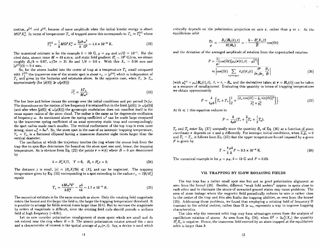

Fig 2b
Fiq 1amp
~ Fig lh
Magnetic Trap Center
I 1
Fig 2c
1r
~g__ 0Ll I 1--- t
Fig 2a