09/20/04 introducing proteins into genetic algorithms – csimta'04 introducing “proteins”...

09/20/04 Introducing Proteins into Genetic Algorithms – CSIMTA'04

Introducing “Proteins” into Genetic Algorithms

Virginie LEFORT, Carole KNIBBE, Guillaume BESLON, Joël FAVREL

INSA-IF/PRISMa, FRANCEArtificial Life and Behaviour Team (ALAB)

2


Introduction: Origin of species Natural (Darwinian) evolution

Variation of the genotype ( variation of the phenotype) Extinction of the less fitted individuals Preservation (and diffusion) of favourable variations Rejection of unfavourable variations

Information support (genotype) DNA Genes (DNA coding sequences)

Genotype to phenotype mapping (simplified!) Transcription-translation (genes proteins) Biochemistry (proteins cells)

3


Principle of genetic algorithms Mimic darwinian evolution in the context of

parametric optimization All parameters are aligned to build a (genetic) sequence An artificial population is randomly generated Individuals reproduce themselves (generation loop) Selection mechanism based on a fitness function The genetic sequence can be modified during the

reproduction process (Mutations, Crossover)

Genetic algorithms are very efficient They can be applied to a wide range of problems

even when no a priori knowledge is available

4


Principles of genetic algorithms The reproduction loop :

Selection

Reproduction

Fitness Evaluation

5


But ... The genotype structure is chosen initially (and

arbitrarily) The genotype structure constraints the evolutionary

process Close genes evolve together even though the

corresponding parameters are independent Distant genes evolve separately even though the

corresponding parameters are dependent Building blocks hypothesis (J.H. Holland)

The algorithm precision is also chosen initially Precision depends on the parameter encoding Fixed along the overall evolutionary process Precision generally is the same for all parameters

6


Why ? The genotype to phenotype mapping is too simple

one gene one parameter “linear” transformation

The algorithm depends on the genetic structure The genetic structure cannot evolve

Gene 1 Gene 2 Gene 3 Gene 4 Gene 5

Param 1 Param 2 Param 3 Param 4 Param 5

7


Genetic structure constraints In genetic algorithms the genome is directly

mapped into a phenotype The genome structure cannot be modified

Under-specified parameters,

Gene 1 Gene 2 Gene 3 Gene 5

Param 1 Param 2 Param 3 ??? Param 5

8


In genetic algorithms the genome is directly mapped into a phenotype

The genome structure cannot be modified Over-specified parameters,

Gene 1 Gene 2 Gene 3 Gene 4 Gene 5Gene 4’

Param 1 Param 2 Param 3 ??? Param 5

Genetic structure constraints

9


In genetic algorithms the genome is directly mapped into a phenotype

The genome structure cannot be modified Incoherent crossing-over

Gene 3’ Gene 5’ Gene 1’ Gene 4’ Gene 2’


??? ??? ??? Param 4’ ???

Gene 1 Gene 2 Gene 1’ Gene 4’ Gene 2’

Genetic structure constraints

10


… in biology ? In living beings, different genetic structures give

rise to different organisms on the basis of the same translation mechanism …

Genetic principles of the C. Elegans worm are (quite) the same as for bacterias or humans …

The rules are the same in (quite) all the living kingdom …

The gene number, size, position (locus), order … are free to evolve

The information sources are (only) the coding sequences

Why do we loose this property in GAs ?

11


The proteome In biology there is an intermediate level between

the genotype and the phenotype :

The genotype structureis lost …

Genotype and phenotype structures can evolve separately ...Phenotype


Proteome

12


The RBF-Gene algorithm: Basic ideas Back to the “biological” gene definition

The genome is a succession of coding and non-coding sequences

Coding sequences (genes) are identified by their local context

Each gene expresses a protein whose function is “only” determined by the local sequence

The local sequence is translated thanks to a “genetic code” Proteins interact to produce the phenotype

The RBF-Gene model is based on: A “protein layer” between genotype and phenotype A “genetic” code to find the genes and the associated

“protein” functions

13


Our “protein” layer The phenotype is an Rn Rm function (regression function) The RBF-Gene model introduces an intermediate layer

between the parameters and the regression function The function is a linear combination of elementary kernel functions The kernel shape is predefined (e.g. gaussian functions, sinus, …) one coding sequence (one gene) one kernel (event. not effective) The genetic code is used to translate the gene sequence into kernel

parameters

Example: R R gaussian kernels Three parameters/kernel : μi, σi and wi

The final phenotype is given by :

μ

σ

Kernel Ki

n

iii Kw

1

14


The genetic code Biological genetic code

4 bases (A, C, G, T) 64 codons (3 bases) 4 specific codons : Start (‘ATG’) and Stop (‘TAA’, ‘TAG’ and ‘TGA’) 20 amino-acids

RBF-Gene genetic code Simplification : direct use of the “DNA” bases (n bases) 2 specific bases : Start (‘A’) and Stop (‘B’) 2 bases for each kernel parameter (e.g. ‘C’ and ‘D’ for parameter

w) The number of bases depends on the number of parameters (i.e.

on the function dimension) Binary, variable length Gray code ...

15


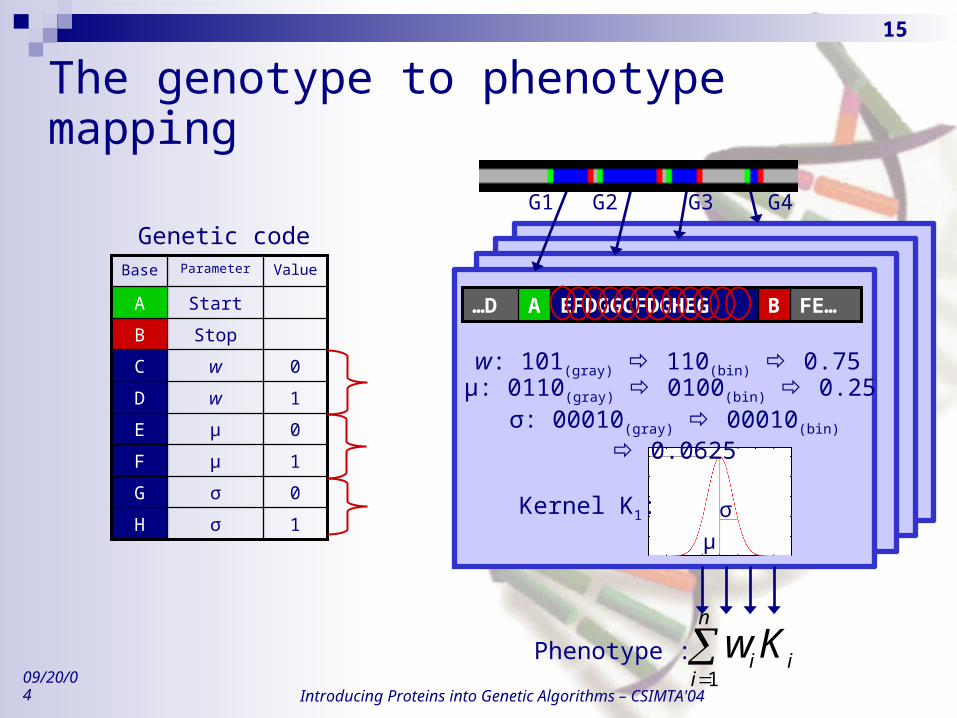
G2 G3 G4

The genotype to phenotype mapping

G1

FE…BEFDGGCFDGHEGA…D

μ

σKernel K1:

σ: 00010(gray) 00010(bin) 0.0625

Phenotype :

n

iii Kw

1

1σH

0σG

1μF

0μE

1wD

0wC

StopB

StartA

ValueParameterBase

Genetic code

w: 101(gray) 110(bin) 0.75μ: 0110(gray) 0100(bin) 0.25

16


The reproduction loop General Principle: Same as GAs

Biologically inspired operators (local, global, …)

Fitness Evaluation

Selection

Reproduction

17


Advantages of the RBF-Gene model The regression function is computable whatever the

genome structure (size, genes number, genes order, …) The algorithm is (partly) problem-independant

The algorithm adapts the gene number The algorithm can adapt the phenotype complexity

The algorithm adapts the gene length The algorithm can adapt the phenotype precision The algorithm can enhance the precision during the

evolutionary process

The “protein” layer enables us to analyse the phenotype

E.g. One kernel one fuzzy rule

18


Example: regression on a “toy-problem”

• Composition of 5 gaussian functions• Gaussian noise : =0.05• Two example sets :

• Learning set (50 points)• Validation set (50 points)

• Parameters :• Population size : 100• Initial genome size : 200• Number of codons : 8• Mutation rate : 5.10-4 / base• Indel rate : 2 x 5. 10-4 / base• Rearrangement rate : 3 x 0.02 / indiv.• Crossing-over rate : 0.6 / indiv.

• Fitness criteria : mean square error

19


Results (1): Evolution of the fitness

20


Results (2): Genome, “proteome” and phenotypeGeneration: 0

Initial population :• Genome size : 200• Number of kernels: 16 (4 coding)• Learning fitness: 1.3612• Validation fitness: 1.0056

Final results :• Genome size : 472• Number of kernels: 15 (10 coding)• Learning fitness: 0.0206• Validation fitness: 0.0497

Generation: 2000

21


Results (2): “proteome” and phenotypeGeneration: 2000

22


Results (3): Overfitting

23


Results (3): Overfitting

24


Results (4): Genome size

25


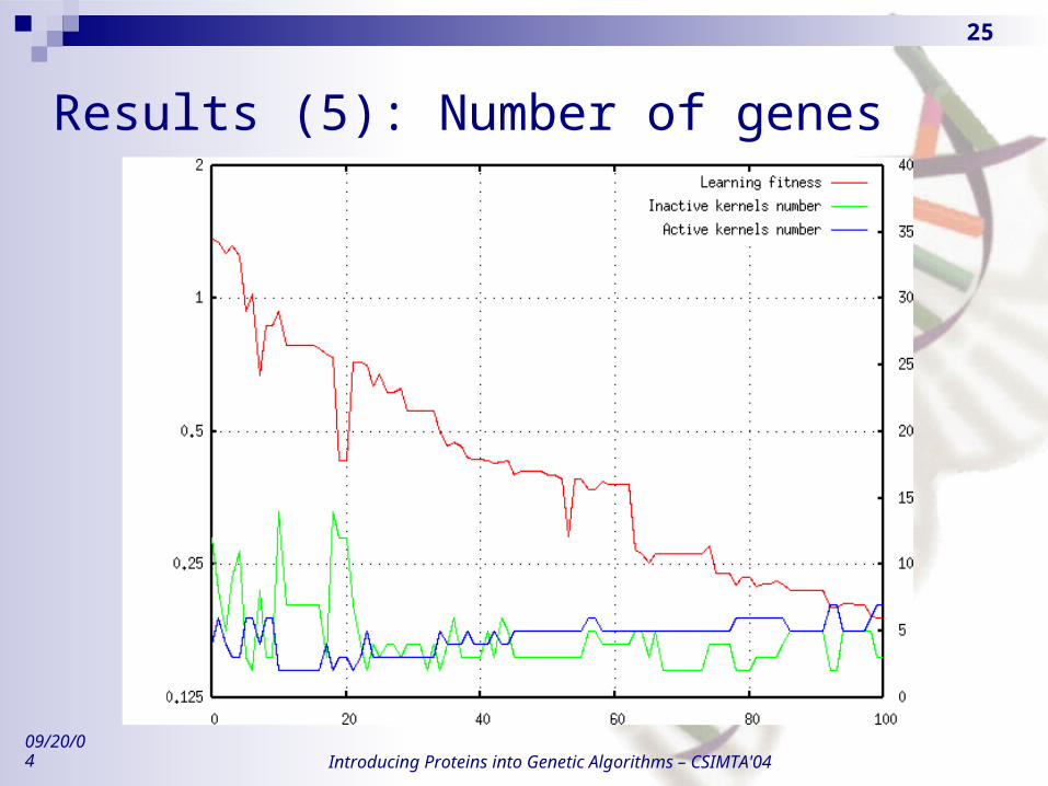
Results (5): Number of genes

26


Results (6): Gene size (i.e. precision)

27


Results (7): Coding proportion

28


Conclusion

Reorganization of the genome DURING and BY the evolutionary process The algorithm adapts the gene number The algorithm adapts the gene size

Tested on the abalone dataset (R8 to R regression) Very good results (but slow computations)

Perspectives: Evolution of neural networks The final structure is an RBF-Network … Other architectures are possible (MLP, recurrent networks, …) The algorithm adapts the synaptic weights and the network structure

(e.g. number of neurons) Rules extraction from the proteome

29


Questions ?

09/20/04 introducing proteins into genetic algorithms – csimta'04 introducing “proteins”...

Documents

crossover genetic algorithms

genetic sequence

genome structure

genotype structure constraints

available slide

genotype variation

corresponding parameters

phenotype mapping