IV Estimation

A. Using instruments by augmenting VARB. Using instruments external to VAR (Stock

and Watson, 2012)C. Using IV for mixed-frequency inference:

Gertler and Karadi (2015)D. Augmented VAR versus IV estimationE. Natural experiments in macro (Fuchs-

Schuendeln and Hassan, 2015)

1

2

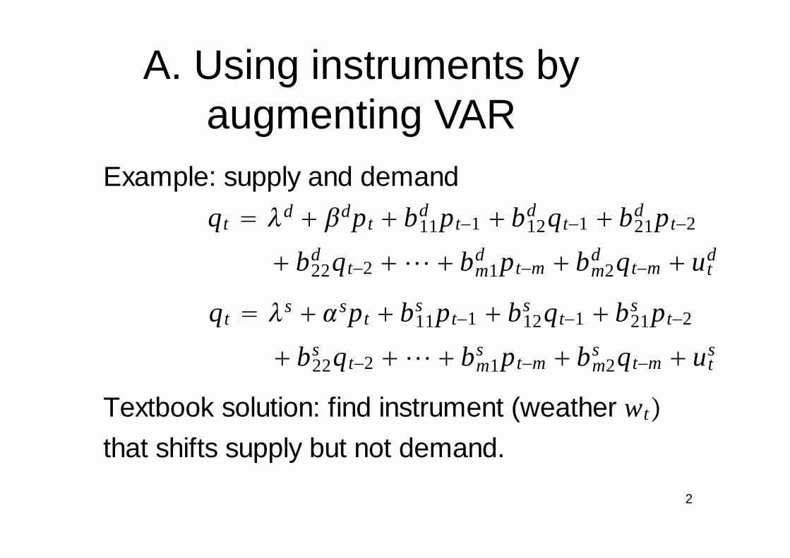
A. Using instruments by augmenting VAR

Example: supply and demand

qt � �d � �dpt � b11d pt�1 � b12

d qt�1 � b21d pt�2

� b22d qt�2 � � � bm1

d pt�m � bm2d qt�m � ut

d

qt � �s � �spt � b11s pt�1 � b12

s qt�1 � b21s pt�2

� b22s qt�2 � � � bm1

s pt�m � bm2s qt�m � ut

s

Textbook solution: find instrument (weather wt�

that shifts supply but not demand.

3

yt � �qt ,pt,wt��

qt � �d � �dpt � �1d�yt�1 � � � �m

d�yt�m � utd

qt � �s � �spt � hswt � �1s�yt�1 � � � �m

s�yt�m � uts

wt � �w � �1w�yt�1 � � � �m

w�yt�m � utw

Could impose additional restrictions on � ji

4

Ay t � � � B1yt�1 � � � Bmyt�m � ut

E�utut�� � D (diagonal)

A �

1 ��d 0

1 ��s �hs

0 0 1

5

Algorithm 1: Find �� MLEd ,��MLE

s ,ĥMLEs by

maximizing log likelihood numerically

�T/2� log|A|2 � �T/2� log|D|

��T/2�trace��A �D�1A��� �

Estimates will satisfy

D� � �� �(diagonal)

6

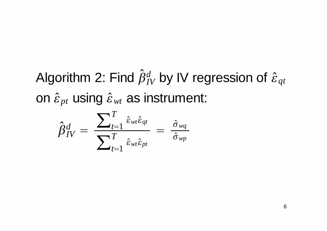
Algorithm 2: Find �� IVd by IV regression of �� qt

on �� pt using ��wt as instrument:

�� IVd �

�t�1T

��wt��qt

�t�1T

��wt��pt

��� wq

�� wp

7

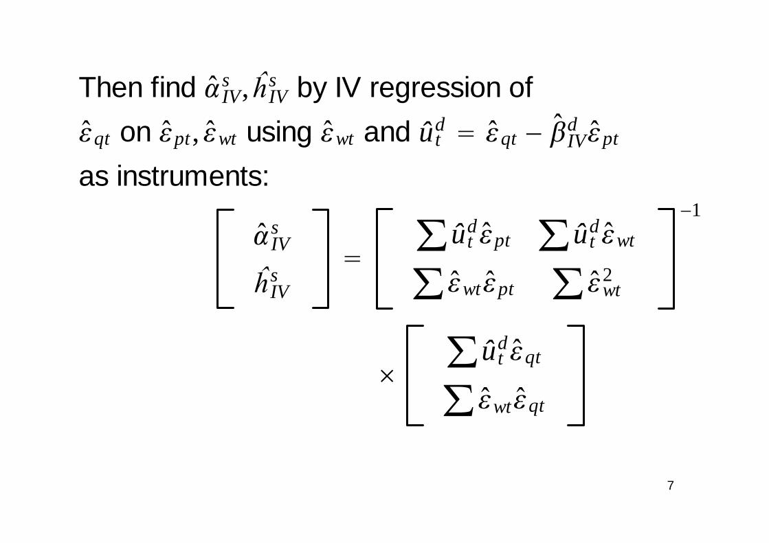
Then find �� IVs ,ĥIV

s by IV regression of

�� qt on �� pt,��wt using ��wt and ûtd � �� qt � �� IV

d �� pt

as instruments:

�� IVs

ĥ IVs

��ût

d�� pt �ûtd��wt

���wt�� pt ���wt2

�1

��ût

d�� qt

���wt�� qt

8

Proposition: the estimates of the two

algorithms are numerically identical.

Proof:

�ûtd��wt � 0 by definition of �� IV

d

�ûtsût

d � �ûts��wt � 0 by definition of �� IV

s ,ĥ IVs

 IV��  IV�

is diagonal

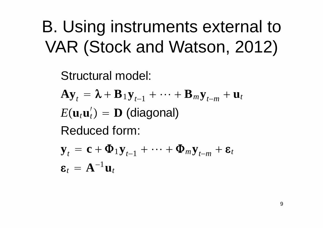
B. Using instruments external to VAR (Stock and Watson, 2012)

9

Structural model:

Ay t � � � B1yt�1 � � � Bmyt�m � ut

E�utut�� � D (diagonal)

Reduced form:

yt � c � �1yt�1 � � � �myt�m � � t

� t � A �1ut

10

Suppose we have instrument zit that is

relevant: E�zituit� � � i � 0

valid: E�zitujt� � 0 for i � j

11

Under the above assumptions,

E�� tzit� � A �1E�utzit� � A �1� i ei

ei � col i of I n

so can estimate ith column of

A �1 (up to unknown constant) by

ã�i � � T�1 �t�1T �� tzit

12

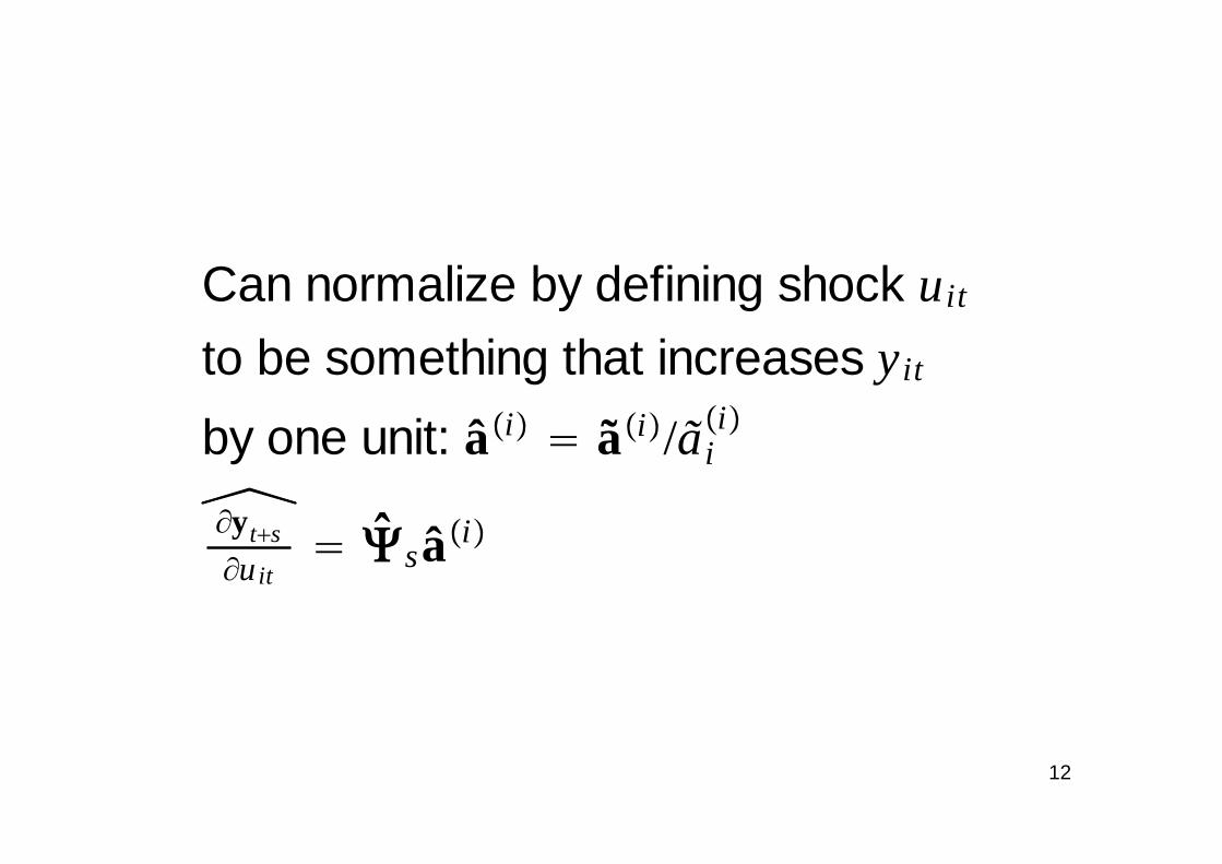
Can normalize by defining shock uit

to be something that increases yit

by one unit: â�i� � ã�i �/ãi�i�

�yt�s

�uit� �� sâ�i �

13

Can also estimate ûit as follows.

Suppose we observed ut and

regressed zit on ut:

zit � � i�ut � vit

plim �� i � �� i /dii �ei

14

If instead we regressed zit on � t,

zit � � i�� t � vit

this would just be rotation of

above regression since � t � A �1ut

Hence fitted values from regression

of zit on �� t give consistent estimate

of �� i /dii �uit

Stock-Watson examined several different proposed measures of monetary policy shocks, including

(1) Romer-Romer shocks(2) Monetary policy shocks inferred

from Smets-Wouters empirical DGSE(3) Gürkaynak-Sack-Swanson (2005)

Fed target shock

15

Structural IRF using Romer-Romer monetary shocks

16

Structural IRF using Smets-Wouters monetary shocks

17Correlation between RR and SW shock = 0.09

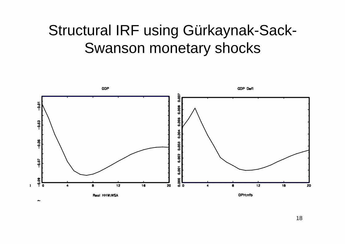
Structural IRF using Gürkaynak-Sack-Swanson monetary shocks

18

19

Stock-Watson considered 17 different instruments for 6 structural shocks

20

Instruments should be correlated within group and not across groups

• Most important shocks in Great Recession seemed to be financial shocks

• TED spread = 3-month LIBOR rate (an average of interest rates offered in the London interbank market for 3-month dollar-denominated loans) and the 3-month Treasury bill rate

• Gilchrist-Zakrajšek spread = average gap between corporate and risk-free yields

21

Historical decomposition: contribution of financial shocks (TED)

22

C. Using IV for mixed-frequency inference: Gertler and Karadi (2015)

• Monthly 1979:M7 – 2012:M6• interest rate on 1-year U.S. Treasury

(takes place of fed funds rate in older regressions)

• log of CPI• log of industrial production• Gilchrist-Zakrajšek spread

23

Instruments for monetary policy shock

(1) Kuttner’s surprise component of change in current-month fed funds futures contract in 30-minute window around FOMC announcement in month t• = 0 if no announcement• Only estimate over ℚ = {[1991:M1 –

2008:M6] U [2009:M7 – 2012:M6]}• Identifies linear combination of reduced-

form VAR residuals that is to be designated “monetary policy shock”

24

Instruments for monetary policy shock

(2) Change in 3-month ahead fed funds futures contract in 30-minute window around FOMC announcement in month t

(3)-(5) Change in 6, 9, and 12-month ahead 3-month Eurodollar futures in 30 minute window in month t

25

26

� t � reduced-form VAR residuals

(�1t � error forecasting 1-year interest rate)

ut � structural shocks

(u1t � monetary policy shock�

zt � �5 � 1� vector of instruments

27

� t � A �1ut

��t

�u1t� a�1� (col 1 of A �1�

Estimate jth element of a�1� by 2SLS

regression of �� jt on �� 1t using zt as inst

aj�1�

��

t���� jt�� 1t

�t��

�� 1t2

�� 1t � ���zt

�� � �t��

ztzt� �

t��zt�� 1t

�yt�s

�u1t� �sa�1�

28

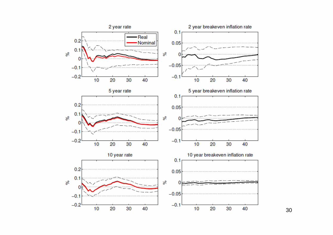
• Next consider 5-variable VARs, where alternative interest rate measures are added, one at a time

29

30

D. Augmented VAR versus IV estimation

31

1) advantage of augmented VAR:

structural shock can be linear combination

of innovations to yt and zt, not just

innovations to yt

2) advantage of using Stock-Watson IV:

can use longer sample to estimate

nonorthogonalized IRF �s than for a�i �

Nonorthogonalized IRF for 1960:Q1-1990:Q4 sample

Response of GDP to fed funds

0 5 10 15-1.50

-1.25

-1.00

-0.75

-0.50

-0.25

0.00

0.25

Response of inflation to fed funds

0 5 10 15-0.25-0.20-0.15-0.10-0.05-0.000.050.100.150.20

Response of fed funds to fed funds

0 5 10 15-0.2

0.0

0.2

0.4

0.6

0.8

1.0

32

Nonorthogonalized IRF for 1991:Q1-2007:Q4 sample

33

Response of GDP to fed funds(1991:1-2007:4)

0 5 10 15-0.8

-0.6

-0.4

-0.2

-0.0

0.2

0.4

Response of inflation to fed funds(1991:1-2007:4)

0 5 10 15-0.3-0.2-0.10.00.10.20.30.40.50.6

Response of fed funds to fed funds(1991:1-2007:4)

0 5 10 15-0.250.000.250.500.751.001.251.501.75

Nonorthogonalized IRF for 1954:Q3-2007:Q4 sample

34

Response of GDP to fed funds(1954:3-2007:4)

0 5 10 15-1.4-1.2-1.0-0.8-0.6-0.4-0.2-0.00.2

Response of inflation to fed funds(1954:3-2007:4)

0 5 10 15-0.20-0.15-0.10-0.05-0.000.050.100.150.200.25

Response of fed funds to fed funds(1954:3-2007:4)

0 5 10 15-0.2

0.0

0.2

0.4

0.6

0.8

1.0

1.2

Barakchian and Crowe (JME, 2013)

35

36

Barakchian and Crowe augmented VAR with accumulated shocks

37

E. Natural experiments in macro

• Application: permanent-income hypothesis• Change in income at t that was perfectly

anticipated at t – 1 should have no effect on consumption at date t

• If find effect it is evidence of borrowing constraints or some departure from neoclassical assumptions

38

2001 Bush tax rebates (Johnson, Parker, Souleles, AER 2006; Agarwal

and Souleles, JPE 2007)• Households notified by letter months in

advance of $300-$600 rebates; substantial press coverage

• Checks delivered over 10-week period based on social security numbers

• Each dollar of rebate added 37¢ in nondurable spending within 3 months of receiving rebate

39

2008 Economic Stimulus Act rebates (Parker, Souleles, Johnson,

McClelland, AER 2013)• Rebates of $300-$1200 rebates• Checks delivered or funds wired based on

social security numbers• Each dollar of rebate added 12¢ in

nondurable spending within 3 months of receiving rebate (statistically significant)

40

Aaronson, Agarwal French (2012)

minimum wage reject

Agarwal and Qian 2011 Singapore growth dividends

cannot reject

Browning and Collado(2011)

Spanish bonus payments scheme

cannot reject

Coulibably and Li (2006) last mortgage payment cannot reject

Hsieh (2003) Alaska permanent fund cannot reject

Scholnick (2013) last mortgage payment reject

Shea (1995) union wage agreement reject

Stephens (2008) last auto payment reject

Stephens (2003) Social Security day of month

reject

Wilcox (1989) Social Security changes reject41

42