05 machine learning - supervised fisher classifier

Machine Learning for Data MiningFisher Linear Discriminant

Andres Mendez-Vazquez

May 26, 2015

1 / 43

Outline

1 IntroductionHistoryThe Rotation IdeaClassifiers as Machines for dimensionality reduction

2 SolutionUse the mean of each ClassScatter measureThe Cost FunctionA Transformation for simplification and defining the cost function

3 Where is this used?Applications

4 Relation with Least Squared ErrorWhat?

2 / 43

Outline

3 / 43

Outline

4 / 43

Rotation

ProjectingProjecting well-separated samples onto an arbitrary line usually produces aconfused mixture of samples from all of the classes and thus produces poorrecognition performance.

Something NotableHowever, moving and rotating the line around might result in anorientation for which the projected samples are well separated.

Fisher linear discriminant (FLD)It is a discriminant analysis seeking directions that are efficient fordiscriminating binary classification problem.

5 / 43

Rotation

5 / 43

Rotation

5 / 43

Example

Example - From Left to Right the Improvement

6 / 43

Outline

7 / 43

This is actually coming from...

Classifier asA machine for dimensionality reduction.

Initial SetupWe have:

Nd-dimensional samples x1, x2, ..., xN .Ni is the number of samples in class Ci for i=1,2.

Then, we ask for the projection of each xi into the line by means of

yi = wT xi (1)

8 / 43

yi = wT xi (1)

8 / 43

yi = wT xi (1)

8 / 43

yi = wT xi (1)

8 / 43

yi = wT xi (1)

8 / 43

Outline

9 / 43

Use the mean of each Class

ThenSelect w such that class separation is maximized

We then define the mean sample for ecah class1 C1 ⇒m1 = 1

∑N1i=1 xi

2 C2 ⇒m2 = 1N2

∑N2i=1 xi

Ok!!! This is giving us a measure of distanceThus, we want to maximize the distance the projected means:

m1 −m2 = wT (m1 −m2) (2)

where mk = wT mk for k = 1, 2.

10 / 43

∑N1i=1 xi

2 C2 ⇒m2 = 1N2

∑N2i=1 xi

m1 −m2 = wT (m1 −m2) (2)

10 / 43

∑N1i=1 xi

2 C2 ⇒m2 = 1N2

∑N2i=1 xi

m1 −m2 = wT (m1 −m2) (2)

10 / 43

∑N1i=1 xi

2 C2 ⇒m2 = 1N2

∑N2i=1 xi

m1 −m2 = wT (m1 −m2) (2)

10 / 43

∑N1i=1 xi

2 C2 ⇒m2 = 1N2

∑N2i=1 xi

m1 −m2 = wT (m1 −m2) (2)

10 / 43

However

We could simply seek

wT (m1 −m2)

s.t.d∑

i=1wi = 1

After allWe do not care about the magnitude of w.

11 / 43

However

We could simply seek

wT (m1 −m2)

s.t.d∑

i=1wi = 1

After allWe do not care about the magnitude of w.

11 / 43

Example

Here, we have the problem... The Scattering!!!

12 / 43

Outline

13 / 43

Fixing the Problem

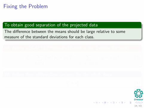
To obtain good separation of the projected dataThe difference between the means should be large relative to somemeasure of the standard deviations for each class.

We define a SCATTER measure (Based in the Sample Variance)

∑xi∈Ck

(wT xi −mk

∑yi=wT xi∈Ck

(yi −mk)2 (3)

We define then within-class variance for the whole data

s21 + s2

14 / 43

Fixing the Problem

∑xi∈Ck

(wT xi −mk

∑yi=wT xi∈Ck

(yi −mk)2 (3)

s21 + s2

14 / 43

Fixing the Problem

∑xi∈Ck

(wT xi −mk

∑yi=wT xi∈Ck

(yi −mk)2 (3)

s21 + s2

14 / 43

Outline

15 / 43

Finally, a Cost Function

The between-class variance

(m1 −m2)2 (5)

The Fisher criterionbetween-class variancewithin-class variance (6)

Finally

J (w) = (m1 −m2)2

s21 + s2

16 / 43

(m1 −m2)2 (5)

Finally

J (w) = (m1 −m2)2

s21 + s2

16 / 43

(m1 −m2)2 (5)

Finally

J (w) = (m1 −m2)2

s21 + s2

16 / 43

Outline

17 / 43

We use a transformation to simplify our lifeFirst

J (w) =

(wT m1 − wT m2

)2∑yi =wT xi ∈C1

(yi − mk)2 +∑

yi =wT xi ∈C2(yi − mk)2

Second

J (w) =

(wT m1 − wT m2

)(wT m1 − wT m2

)T∑yi =wT xi ∈C1

(wT xi − mk

)(wT xi − mk

)T+∑

yi =wT xi ∈C2

(wT xi − mk

)(wT xi − mk

J (w) =wT (m1 − m2)

(wT (m1 − m2)

wT (xi − m1)(

wT (xi − m1))T

yi =wT xi ∈C2wT (xi − m2)

(wT (xi − m2)

18 / 43

J (w) =

(wT m1 − wT m2

(yi − mk)2 +∑

Second

J (w) =

(wT m1 − wT m2

)(wT m1 − wT m2

(wT xi − mk

)(wT xi − mk

)T+∑

yi =wT xi ∈C2

(wT xi − mk

)(wT xi − mk

J (w) =wT (m1 − m2)

(wT (m1 − m2)

wT (xi − m1)(

wT (xi − m1))T

(wT (xi − m2)

18 / 43

J (w) =

(wT m1 − wT m2

(yi − mk)2 +∑

Second

J (w) =

(wT m1 − wT m2

)(wT m1 − wT m2

(wT xi − mk

)(wT xi − mk

)T+∑

yi =wT xi ∈C2

(wT xi − mk

)(wT xi − mk

J (w) =wT (m1 − m2)

(wT (m1 − m2)

wT (xi − m1)(

wT (xi − m1))T

(wT (xi − m2)

18 / 43

Transformation

Fourth

J (w) =wT (m1 − m2) (m1 − m2)T w∑

yi =wT xi ∈C1wT (xi − m1) (xi − m1)T w +

∑yi =wT xi ∈C2

wT (xi − m2) (xi − m2)T w(11)

FifthJ (w) =

wT (m1 − m2) (m1 − m2)T w

wT[∑

yi =wT xi ∈C1(xi − m1) (xi − m1)T +

∑yi =wT xi ∈C2

(xi − m2) (xi − m2)T]

Now Rename

J (w) = wT SBwwT Sww (13)

19 / 43

Transformation

Fourth

J (w) =wT (m1 − m2) (m1 − m2)T w∑

∑yi =wT xi ∈C2

wT (xi − m2) (xi − m2)T w(11)

FifthJ (w) =

wT (m1 − m2) (m1 − m2)T w

wT[∑

∑yi =wT xi ∈C2

(xi − m2) (xi − m2)T]

Now Rename

19 / 43

Transformation

Fourth

J (w) =wT (m1 − m2) (m1 − m2)T w∑

∑yi =wT xi ∈C2

wT (xi − m2) (xi − m2)T w(11)

FifthJ (w) =

wT (m1 − m2) (m1 − m2)T w

wT[∑

∑yi =wT xi ∈C2

(xi − m2) (xi − m2)T]

Now Rename

19 / 43

Derive with respect to w

ThusdJ (w)

dw =d(wT SBw

) (wT Sww

dw = 0 (14)

dJ (w)dw =

(SBw + ST

B w) (

wT Sww)−1 −

(wT SBw

) (wT Sww

)−2 (Sww + STw w)

= 0(15)

Now because the symmetry in SB and Sw

dJ (w)dw = SB

(wT Sww) − wT SBwSww(wT Sww)2 = 0 (16)

20 / 43

ThusdJ (w)

dw =d(wT SBw

) (wT Sww

dw = 0 (14)

dJ (w)dw =

(SBw + ST

B w) (

wT Sww)−1 −

(wT SBw

) (wT Sww

)−2 (Sww + STw w)

= 0(15)

dJ (w)dw = SB

20 / 43

ThusdJ (w)

dw =d(wT SBw

) (wT Sww

dw = 0 (14)

dJ (w)dw =

(SBw + ST

B w) (

wT Sww)−1 −

(wT SBw

) (wT Sww

)−2 (Sww + STw w)

= 0(15)

dJ (w)dw = SB

20 / 43

ThusdJ (w)

dw = SB

Then (wT Sww

)SBw =

(wT SBw

)Sww (18)

21 / 43

ThusdJ (w)

dw = SB

Then (wT Sww

)SBw =

(wT SBw

)Sww (18)

21 / 43

Now, Several Tricks!!!

FirstSBw = (m1 − m2) (m1 − m2)T w = α (m1 − m2) (19)

Where α = (m1 −m2)T w is a simple constantIt means that SBw is always in the direction m1 −m2!!!

In additionwT Sww and wT SBw are constants

22 / 43

Finally

Sww ∝ (m1 −m2)⇒ w ∝ S−1w (m1 −m2) (20)

Once the data is transformed into yi

Use a threshold y0 ⇒ x ∈ C1 iff y (x) ≥ y0 or x ∈ C2 iff y (x) < y0

Or ML with a Gussian can be used to classify the new transformeddata using a Naive Bayes (Central Limit Theorem and y = wT x sumof random variables).

23 / 43

Finally

Sww ∝ (m1 −m2)⇒ w ∝ S−1w (m1 −m2) (20)

23 / 43

Finally

Sww ∝ (m1 −m2)⇒ w ∝ S−1w (m1 −m2) (20)

23 / 43

Outline

24 / 43

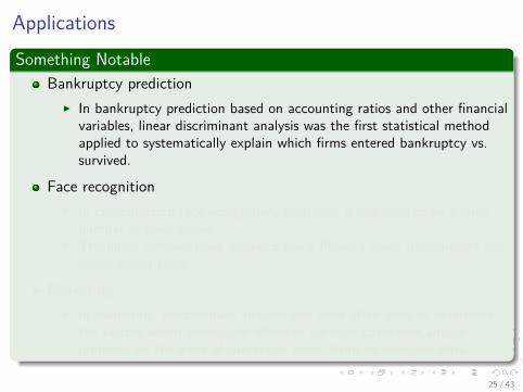
ApplicationsSomething Notable

Bankruptcy predictionI In bankruptcy prediction based on accounting ratios and other financial

variables, linear discriminant analysis was the first statistical methodapplied to systematically explain which firms entered bankruptcy vs.survived.

Face recognitionI In computerized face recognition, each face is represented by a large

number of pixel values.I The linear combinations obtained using Fisher’s linear discriminant are

called Fisher faces.

MarketingI In marketing, discriminant analysis was once often used to determine

the factors which distinguish different types of customers and/orproducts on the basis of surveys or other forms of collected data.

25 / 43

Applications

Something NotableBiomedical studies

I The main application of discriminant analysis in medicine is theassessment of severity state of a patient and prognosis of diseaseoutcome.

26 / 43

Applications

Something NotableBiomedical studies

I The main application of discriminant analysis in medicine is theassessment of severity state of a patient and prognosis of diseaseoutcome.

26 / 43

Please

Your Reading Material, it is about the Multi-class4.1.6 Fisher’s discriminant for multiple classes AT “Pattern Recognition”by Bishop

27 / 43

Outline

28 / 43

Relation with Least Squared Error

FirstThe least-squares approach to the determination of a linear discriminantwas based on the goal of making the model predictions as close aspossible to a set of target values.

SecondThe Fisher criterion was derived by requiring maximum class separation inthe output space.

29 / 43

Relation with Least Squared Error

FirstThe least-squares approach to the determination of a linear discriminantwas based on the goal of making the model predictions as close aspossible to a set of target values.

SecondThe Fisher criterion was derived by requiring maximum class separation inthe output space.

29 / 43

How do we do this?

FirstWe have N samples.We have N1samples for class C1.We have N2 samples for class C2.

So, we decide the following for the targets on each classWe have then for class C1 is N

We have then for class C2 is − NN2

30 / 43

How do we do this?

30 / 43

How do we do this?

30 / 43

How do we do this?

30 / 43

The new cost function

E = 12

N∑n=1

(wT xn + wo − tn

)2(21)

Deriving with respect to wN∑

(wT xn + wo − tn

)xn = 0 (22)

Deriving with respect to w0

N∑n=1

(wT xn + wo − tn

)= 0 (23)

31 / 43

E = 12

N∑n=1

(wT xn + wo − tn

)2(21)

(wT xn + wo − tn

)xn = 0 (22)

N∑n=1

(wT xn + wo − tn

)= 0 (23)

31 / 43

E = 12

N∑n=1

(wT xn + wo − tn

)2(21)

(wT xn + wo − tn

)xn = 0 (22)

N∑n=1

(wT xn + wo − tn

)= 0 (23)

31 / 43

We have thatN∑

(wT xn + wo − tn

N∑n=1

(wT xn + wo

N∑n=1

(wT xn + wo

)−N1

+ N2NN2

(wT xn + wo

Then ( N∑n=1

)+ Nwo = 0

32 / 43

We have thatN∑

(wT xn + wo − tn

N∑n=1

(wT xn + wo

N∑n=1

(wT xn + wo

)−N1

+ N2NN2

(wT xn + wo

Then ( N∑n=1

)+ Nwo = 0

32 / 43

We have that

wo = −wT(

N∑n=1

We rename 1N∑N

n=1 xn = m

m = 1N

N∑n=1

xn = 1N [N1m1 + N2m2]

Finally

wo = −wT m

33 / 43

We have that

wo = −wT(

N∑n=1

We rename 1N∑N

n=1 xn = m

m = 1N

N∑n=1

xn = 1N [N1m1 + N2m2]

Finally

wo = −wT m

33 / 43

We have that

wo = −wT(

N∑n=1

We rename 1N∑N

n=1 xn = m

m = 1N

N∑n=1

xn = 1N [N1m1 + N2m2]

Finally

wo = −wT m

33 / 43

In a similar wayN∑

(wT xn + wo

)xn −

N∑n=1

tnxn = 0

34 / 43

Thus, we have

Something NotableN∑

(wT xn + wo

)xn −

N1∑n=1

xn + NN2

N2∑n=1

xn = 0

ThusN∑

(wT xn + wo

)xn −N (m1 −m2) = 0

35 / 43

Thus, we have

Something NotableN∑

(wT xn + wo

)xn −

N1∑n=1

xn + NN2

N2∑n=1

xn = 0

ThusN∑

(wT xn + wo

)xn −N (m1 −m2) = 0

35 / 43

ThenN∑

(wT xn −wT m

)xn = N (m1 −m2)

Thus [ N∑n=1

(wTxn −wT m

]= N (m1 −m2)

NowWhat? Please do this as a take homework for next class

36 / 43

ThenN∑

(wT xn −wT m

)xn = N (m1 −m2)

Thus [ N∑n=1

(wTxn −wT m

]= N (m1 −m2)

36 / 43

ThenN∑

(wT xn −wT m

)xn = N (m1 −m2)

Thus [ N∑n=1

(wTxn −wT m

]= N (m1 −m2)

36 / 43

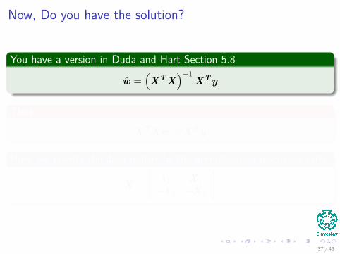
Now, Do you have the solution?

You have a version in Duda and Hart Section 5.8

w =(XTX

)−1XTy

XTXw = XTy

Now, we rewrite the data matrix by the normalization discussed early

11 X1−12 −X2

37 / 43

w =(XTX

)−1XTy

XTXw = XTy

11 X1−12 −X2

37 / 43

w =(XTX

)−1XTy

XTXw = XTy

11 X1−12 −X2

37 / 43

In addition

Our old augmented w

And our new y

y =[ N

38 / 43

In addition

Our old augmented w

And our new y

y =[ N

38 / 43

Thus, we have

Something Notable

1 −1T1

XT1 −XT

] [11 X1

−12 −X2

] [w0w

1T1 −1T

1 −XT2

] [ NN1

Thus, if we use the following definitionsmi = 1

∑x∈Ci x

SW =∑xi∈C1 (xi −m1) (xi −m1)T +

∑xi∈C2 (xi −m2) (xi −m2)T

39 / 43

Thus, we have

Something Notable

1 −1T1

XT1 −XT

] [11 X1

−12 −X2

] [w0w

1T1 −1T

1 −XT2

] [ NN1

∑x∈Ci x

SW =∑xi∈C1 (xi −m1) (xi −m1)T +

39 / 43

Thus, we have

Something Notable

1 −1T1

XT1 −XT

] [11 X1

−12 −X2

] [w0w

1T1 −1T

1 −XT2

] [ NN1

∑x∈Ci x

SW =∑xi∈C1 (xi −m1) (xi −m1)T +

39 / 43

Thus, we have

Something Notable

1 −1T1

XT1 −XT

] [11 X1

−12 −X2

] [w0w

1T1 −1T

1 −XT2

] [ NN1

∑x∈Ci x

SW =∑xi∈C1 (xi −m1) (xi −m1)T +

39 / 43

We have the following

[n (n1m1 + n2m2)T

(n1m1 + n2m2) Sw + n1m1mT1 + n2m2mT

] [w0w

0n [m1 −m2]

nw0 + (n1m1 + n2m2)T w(n1m1 + n2m2) w0 +

[Sw + n1m1mT

1 + n2m2mT2] ] =

n [m1 −m2]

40 / 43

We have the following

[n (n1m1 + n2m2)T

(n1m1 + n2m2) Sw + n1m1mT1 + n2m2mT

] [w0w

0n [m1 −m2]

nw0 + (n1m1 + n2m2)T w(n1m1 + n2m2) w0 +

[Sw + n1m1mT

1 + n2m2mT2] ] =

n [m1 −m2]

40 / 43

We have that

w0 = −wT m[ 1n Sw + n1n2

n2 (m1 −m2) (m1 −m2)T]

w = m1 −m2

ThusSince the vector (m1 −m2) (m1 −m2)T w is in the direction ofm1 −m2

We have thatn1n2n2 (m1 −m2) (m1 −m2)T w = (1− α) (m1 −m2)

41 / 43

We have that

w0 = −wT m[ 1n Sw + n1n2

n2 (m1 −m2) (m1 −m2)T]

w = m1 −m2

41 / 43

We have that

w0 = −wT m[ 1n Sw + n1n2

n2 (m1 −m2) (m1 −m2)T]

w = m1 −m2

41 / 43

Finally

We have that

w = αnS−1w (m1 −m2) (25)

42 / 43

Exercises

BishopChapter 4

4.4, 4.5, 4.6

43 / 43

Exercises

BishopChapter 4

4.4, 4.5, 4.6

43 / 43

05 machine learning - supervised fisher classifier

Engineering