04_v5_gpsfordesigner_ws_4_030402
DESCRIPTION
Work 4TRANSCRIPT

WS4-1CAT509, Workshop 4, March 2002
WORKSHOP 4
BICYCLE PEDAL MESH REFINEMENT AND ADAPTIVITY

WS4-2CAT509, Workshop 4, March 2002

WS4-3CAT509, Workshop 4, March 2002
100 lbs
100 lbs
Elastic Modulus, E 29.0E6 psi
Poisson’s Ratio, 0.3
Density .284 lb/in3
Yield Strength 36,000 psi
WORKSHOP 4 – PEDAL MESH REFINEMENT AND ADAPTIVITY
Problem Description Assume the same 200 lb person riding the bicycle is standing
balanced evenly on each pedal. Material (Steel) properties are as specified below.
Using the previous rough analysis, refine the mesh until you are comfortable with the results. Is this steel strong enough?
Steel ASTM A36
WS4-4CAT509, Workshop 4, March 2002
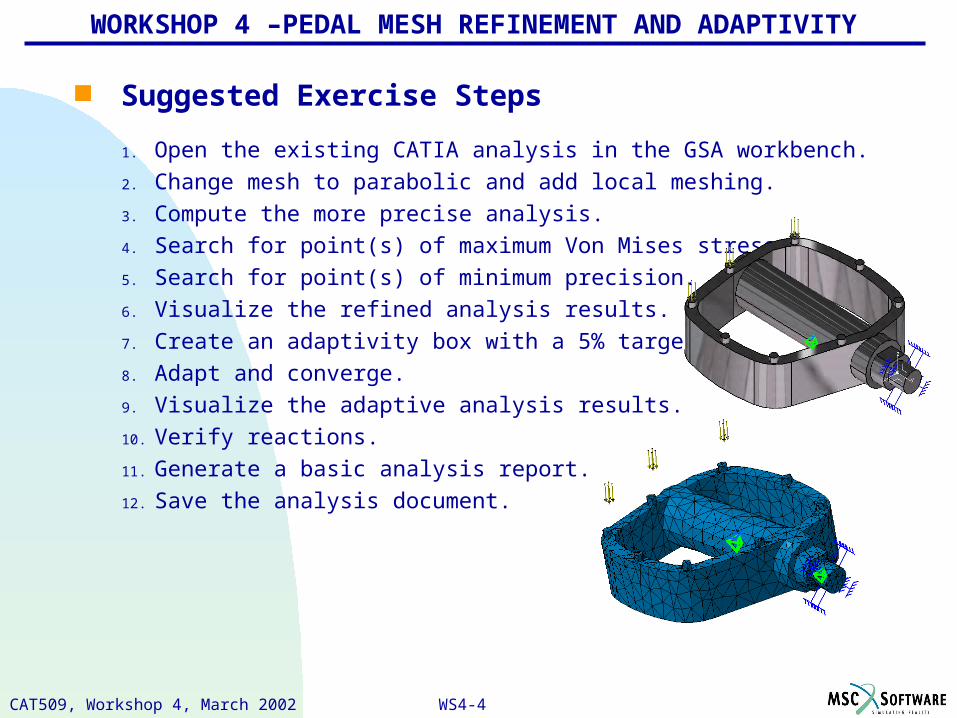
Suggested Exercise Steps
1. Open the existing CATIA analysis in the GSA workbench.
2. Change mesh to parabolic and add local meshing.
3. Compute the more precise analysis.
4. Search for point(s) of maximum Von Mises stress.
5. Search for point(s) of minimum precision.
6. Visualize the refined analysis results.
7. Create an adaptivity box with a 5% target.
8. Adapt and converge.
9. Visualize the adaptive analysis results.
10. Verify reactions.
11. Generate a basic analysis report.
12. Save the analysis document.
WORKSHOP 4 –PEDAL MESH REFINEMENT AND ADAPTIVITY

WS4-5CAT509, Workshop 4, March 2002
Open the CATIA analysis document ws4pedal.CATAnalysis in the Generative Structural Analysis workbench.
Steps:
1. Select File and Open… from the top pull-down menu.
2. Access the class workshop directory using the typical Windows interface.
3. Open the pedal analysis by double-clicking.
By default, the pedal and all other CATAnalysis documents are opened in the Generative Structural Analysis workbench.
Step 1. Open the existing CATIA analysis
1
2
3

WS4-6CAT509, Workshop 4, March 2002
Step 1. Open the existing CATIA analysis
12
.25” Linear Mesh
Max Von Mises 24.6 ksi
Translational Displacement ..00407 inch
Error Estimate 8.65e-8
Global % Precision error
Local % Precision error
43.5 %
NA %
Summary of Workshop 3: the estimated percent error is not low enough (should be less than 10%).
Steps:
1. Double click OCTREE… in the features tree.
2. Note the Global mesh size of .25”, Sag of .025” and Linear element type.
3. Summary of image results.
3

WS4-7CAT509, Workshop 4, March 2002
Step 1. Open the existing CATIA analysis
1
You do not want “auto save” to start while computing a solution, best to turn it off.
Steps:
1. Select Tools from the menu then Options.
2. Select General and the tab General.
3. Deselect the Automatic save button, select OK.
2 3

WS4-8CAT509, Workshop 4, March 2002
Step 2. Change mesh to parabolic and add local meshing
Change the element type from Linear (4-nodes) to Parabolic (10-nodes).
Steps:
1. Select the Change Element Type icon.
2. Select Parabolic then OK.
The best results are achieved using Parabolic elements even though your computation files will be large. Use Linear to locate “hot spots” and to verify a statically determinate model.
21
WS4-9CAT509, Workshop 4, March 2002
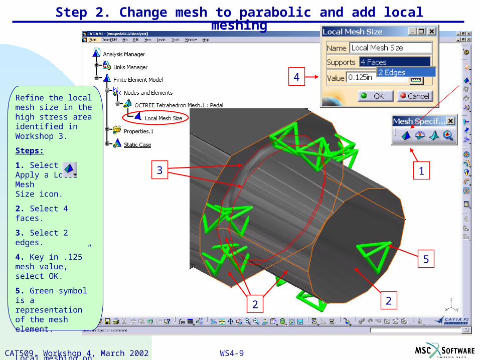
Step 2. Change mesh to parabolic and add local meshing
4
Refine the local mesh size in the high stress area identified in Workshop 3.
Steps:
1. Select the Apply a Local Mesh Size icon.
2. Select 4 faces.
3. Select 2 edges.
4. Key in .125” mesh value, select OK.
5. Green symbol is a representation of the mesh element.
Local meshing on an edge creates nodes along these edges (imposed edges).
22
3
5
1

WS4-10CAT509, Workshop 4, March 2002
Step 2. Change mesh to parabolic and add local meshing
2
4
Refine the local mesh sag size in the high stress area identified in Workshop 3.
Steps:
1. Select the Apply a Local Mesh Sag icon.
2. Select 4 faces.
3. Select 2 edges.
4. Key in .013” sag size (10% of mesh size), select OK.
5. Blue symbol is a representation of sag.
2
5
3 1

WS4-11CAT509, Workshop 4, March 2002
Step 3. Compute the more precise analysis
Important processes to consider before computing:
• RAM on your PC.
• Disk space for the computation.
• Paging space.
• Running with Intel MKL library installed.
See Info Nuggets for details.
Steps:
1. Select the compute icon.
2. Compute All objects, click OK.
3. Note: Intel MKL library found. Click Yes to continue computation.
2
Preview active
3
1
RAM
Available disk space required at your specified external storage location.

WS4-12CAT509, Workshop 4, March 2002
Step 4. Search for point(s) of maximum Von Mises stress
Find the Element with the maximum stress value in the model.
Steps:
1. Clicking on the Von Mises stress icon activates the existing image.
2. Select the Search Extrema icon.
3. Select Global and Local, request 2 maximum at most, then select OK.
It doesn’t look good for our A36 material with 36 ksi yield, but are the values accurate?
2
1
3

WS4-13CAT509, Workshop 4, March 2002
Step 5. Search for point(s) of minimum precision
2
1
3Find the Element with the least accurate value in the model.
Steps:
1. Clicking on the Precision icon deactivates the Von Mises and activates the Estimated local error image.
2. Select the Search Extrema icon.
3. Select Global and Local, request 2 maximum at most, then select OK.
We are looking for very small numbers for the maximum local error, preferably a value of e-8 or lower.

WS4-14CAT509, Workshop 4, March 2002
Step 6. Visualize the refined analysis results
Find the Global estimated error rate percentage value.
Steps:
1. Click on the Information icon.
2. Select activated Estimated local error object in the features tree.
3. Note % error rate (global rate should be 20%, 10% locally).
4. Note the Estimated Precision (this is like epsilon and should be close to zero).
Review information from the other images.
1
2
3
4

WS4-15CAT509, Workshop 4, March 2002
Step 7. Create an adaptivity box with a 10% target
Steps:
1. Activate the Von Mises Image.
2. Click the Adaptivity Box icon.
3. Key in 10% for the Objective Error (this is used in the interest of time 5% is best).
4. Select Extremum button then select Global Maximum.1 from the features tree (this centers the adaptivity box around the Extrema Maximum selected).
5. Manipulate box size and location as shown. The box should encompass the maximum symbols. A small box is recommended due to space and CPU time limits, select OK.
4a
2
1
3
Top
FrontSide
ISO
5
4b

WS4-16CAT509, Workshop 4, March 2002
Step 8. Adapt and converge
2
Allow 2 iterations attempting to achieve the 10% target precision.
Steps:
1. Deactivate all images.
2. Select the Adapt & Converge icon.
3. Key in 2 Iterations, make sure your auto save is turned off: tools + options + general, select OK.
Note: no warnings on RAM, CPU time or space requirements. 1GB of paging space is recommended. This may take 5-7 minutes.
1
3

WS4-17CAT509, Workshop 4, March 2002
Step 9. Visualize the adaptive analysis results
Results for Global precision error.
Steps:
1. Activate the Estimated local error image.
2. Locally update the extrema.
3. Select the info icon then the Est. local error.
4. Improved, meets our suggested 20% max.
Our real interest now is the adaptive local precision.
3
1
2
4

WS4-18CAT509, Workshop 4, March 2002
Step 9. Visualize the adaptive analysis results
Results for adaptive local precision.
Steps:
1. Double click Adaptivty Box.1.
2. Local Error not below 10%, but for this class we will continue with our results.
Time and CPU space permitting you should continue to adapt and converge until you get less than 10%.
Use the compass to move the adaptive box around. Notice the local error will update relative to the elements enclosed by the box.
1
2

WS4-19CAT509, Workshop 4, March 2002
Step 9. Visualize the adaptive analysis results
1
2
Precise maximum Von Mises stress.
Steps:
1. Select the Von Mises icon.
2. Locally update the Extrema object.
3. Double click on Global Max.1 in the features tree.
It might be necessary to delete and recreate Extrema to bring labels out of no show.
3

WS4-20CAT509, Workshop 4, March 2002
Step 9. Visualize the adaptive analysis results
1
3
Check cross sectional area stress values.
Steps:
1. With the Von Mises image active, select the Cut Plane analysis icon.
2. De-select Show cutting plane box.
3. Select the compass at the red dot, drag and locate normal to the shaft as shown.
Analyze various areas using the compass to drag and rotate the cutting plane.
2

WS4-21CAT509, Workshop 4, March 2002
Step 9. Visualize the adaptive analysis results
1
Energy balance value in the adaptive area.
Steps:
1. Activate the Estimated local error image again.
2. All elements are blue, indicating a energy balance of 1.63e-016 Btu (this is zero).
This Btu energy is a result of adding the FEM system forces, similar to epsilon.
2
2

WS4-22CAT509, Workshop 4, March 2002
Step 10. Verify reactions
4
Create an analysis sensor to verify reaction tensors on the clamp.
Steps:
1. Right click Sensor.1 in the features tree and select Create Sensor.
2. Select reaction.
3. Select Clamp.1 then OK (note: ref axis options).
4. Re-compute.
5. Right click Reaction-Clamp.1 in the features tree and select definition.
These values should all add up to zero and match our load applied.
1
2
3
5

WS4-23CAT509, Workshop 4, March 2002
Conclusions The load set of a 200 lb man will overstress the pedal made of A36 steel. Use 4340
material and heat treat to 260-280 BHN for a yield strength equal to 217 ksi. You must change the material type and characteristics in the .CATPart document.
To add a different material to the CATIA material selector or to create your own material catalog see Info Nugget – Materials Catalog.
Step 11. Generate a basic analysis report
.25” Linear Mesh, .025 sag .25”Linear Global Mesh, .025” sag
.125” Parabolic Local Mesh, .013” sag
Adapt and converge target of 5% locally
Max Von Mises 24.6 ksi 172.3 ksi
Translational Displacement .0047 inch .00562 inch
Error Estimate 8.65e-8 Btu 8.4e-16 Btu local
Global % Precision error
Local % Precision error
43.5 %
NA %
18.1 %
12.4 %

WS4-24CAT509, Workshop 4, March 2002
Step 11. Generate a basic analysis report
After activating each image at least once, generate a report.
Steps:
1. Select the Basic Analysis Report icon.
2. Select an Output directory.
3. Key in Title of the report, select OK.
4. Review the HTML report that is created.
1
4
2
3

WS4-25CAT509, Workshop 4, March 2002
Step 12. Save the analysis document
Steps:
1. From the File menu select Save Management.
2. Highlight document you want to save.
3. Select Save As to specify name and path, select OK.
2 3
1

WS4-26CAT509, Workshop 4, March 2002
Info Nugget – Running with the Intel MKL Library
Installing the Intel Library to increase computing time.
Steps:
1. This Intel Library should be downloaded and installed.
2. Example location of installed MKL51B.exe.
You must also add this location to your system “path”. See next page.
http://intel.com/home/tech/resource_library.htm
1
2

WS4-27CAT509, Workshop 4, March 2002
Info Nugget – Running with the Intel MKL Library
1
4
To activate library, add Intel address to your system “Path”.
Steps:
1. Select start + Control Panel + Performance and Maintenance + System + Advanced + Environment Variables.
2. Select “Path” in the System variables, then Edit.
3. Add location to the “path”, select OK, OK,
OK.
4. Result
2
3
WS4-28CAT509, Workshop 4, March 2002
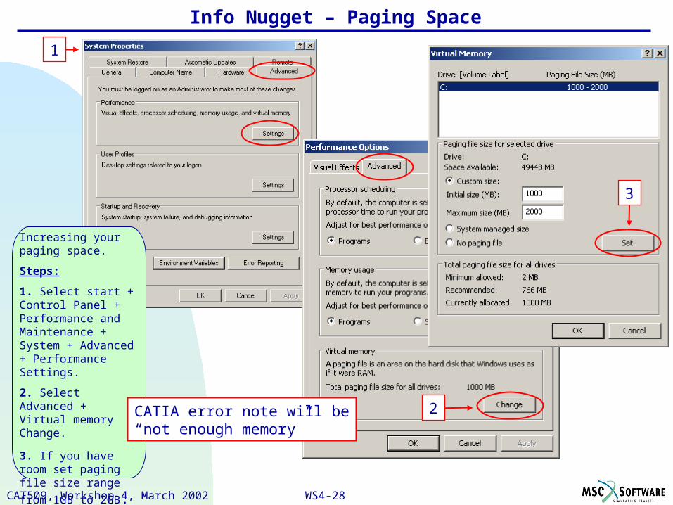
Info Nugget – Paging Space
1
Increasing your paging space.
Steps:
1. Select start + Control Panel + Performance and Maintenance + System + Advanced + Performance Settings.
2. Select Advanced + Virtual memory Change.
3. If you have room set paging file size range
from 1GB to 2GB.
4. Select OK, OK, OK.
2
3
CATIA error note will be“not enough memory”

WS4-29CAT509, Workshop 4, March 2002
Info Nugget – Batch Computing
1
2
3Batch computing. This still seems to use your entire CPU resource unless you have a very powerful PC.
Steps:
1. Copy and Paste a duplicate of the CATIA launch icon on the desktop.
2. Rename to “CNextBatch”.
3. Add “–batch –e CATAnalysisBatch” to
target location.
4. Select OK.
5. Result of double clicking 5
4

WS4-30CAT509, Workshop 4, March 2002
Info Nugget – Material Catalog
1
Edit the existing material catalog.
Steps:
1. Locate the existing Catalog.CATMaterial file by Selecting File + Save management. The path will show if “Link to File” was selected when applying material.
2 Open the file in a CATIA session. The Material Library workbench will start.
3. Edit this file with the various tools provided and save.
3
2

WS4-31CAT509, Workshop 4, March 2002
Info Nugget – Personal Material Catalog
1
3
Steps:
1. Start Material Library workbench.
2. Create all your specific materials with the tools provided.
3. File + Save with the name Catalog.CATMaterial. It must have this exact name to work.
4. Modify Tools + options material catalog path to match where your personal material catalog is filed. This icon will then launch your materials.
2
4

WS4-32CAT509, Workshop 4, March 2002