02transmission planning in liberalised
TRANSCRIPT

CHAPTER 1 – EXECUTIVE SUMMARY
Chapter 1. Executive summary
2
Over the course of the past 20 years, many countries have liberalised their electricity
industries. The historically vertically integrated electricity industry has been broken up
into four parts: generating companies, transmission and distribution network service
providers, and retailers. Reliance has been placed on the forces of competition to
achieve efficient operational and investment decisions by generators, while the
operational and investment of the transmission and distribution networks have been
placed under the responsibility of public utility regulators.
Achieving overall efficient outcomes in this context requires efficient investment by the
regulated transmission network service provider as well as close coordination between
generation and transmission investment. The determination of the optimal sequence and
timing of transmission network investments is known as the transmission planning
problem.
Transmission planning is complex, involving consideration of the impact of a
transmission augmentation under a large number of future demand and supply
scenarios. In principle, the transmission planning problem is well understood in the
context of a vertically-integrated electricity industry, [1]. In this context, a transmission
augmentation has the following primary benefits: It allows for more efficient dispatch
(allowing for lower cost remote generation to be used in place of higher cost local
generation); it allows inefficient investment in generation to be deferred; and it reduces
the need for operating reserves by allowing those reserves to be shared over a wider
area.
In principle, if the liberalised electricity market is sufficiently competitive, the same
tools and techniques that have been developed for transmission planning in the context
of an integrated electricity industry can be applied. However, two new issues arise:
(a) The first is coordination between generation and transmission investment. How
should transmission and generation investment be effectively coordinated?
(b) The second issue is the problem of generator market power. Many
commentators point out that electricity markets are prone to the exercise of
market power. The exercise of market power reduces the efficiency of the
dispatch process, increase the volatility of prices and leads to inefficient over-
investment in generation. In the presence of market power, conventional
Chapter 1. Executive summary
3
transmission planning tools can not easily be applied. In the presence of market
power, in addition to the benefits identified above, transmission augmentations
may also enhance the degree of competition between generators which reduces
the harm associated with market power. The additional benefits of reducing
market power have been referred to as the “competition benefit”.
This thesis focuses on the problem of transmission planning in a liberalised electricity
market in the context of market power.
Although it is widely acknowledged that transmission investment may affect generator
market power, there is as yet no widely accepted methodology for computing the
competition benefits of a transmission augmentation and, in practice, competition
benefits are only estimated on an ad hoc basis, if at all.
This thesis sets out a methodology for modelling market power in the context of
transmission planning. This methodology is based around a multi-level optimisation
problem. The lowest level of this optimisation problem models the dispatch process in a
liberalised electricity market, allowing for generator market power. The solution to this,
the lowest level of the optimisation problem is a Nash equilibria of a simultaneous
move game between the generating companies, taking the transmission network as
given. In this game, generators are able to bid strategically and can choose whether or
not to invest in additional generation capacity.
The upper level of this optimisation problem models the behaviour of the transmission
network service provider. The TNSP is assumed to move first, choosing a configuration
of the transmission network. The TNSP is assumed to select the network configuration
which maximises the TNSP’s objective function for the worst possible Nash
equilibrium of the simultaneous game between the generators. I refer to this as the
“Stackelberg-Worst Nash” optimum.
The remainder of this thesis is organised as follows. The next chapter sets out a
technical introduction to the proposed methodology based on a preliminary
experimental approach. This experiment introduces and tests some concepts which are
used throughout the remainder of the research, and some conclusions are drawn. The
following chapters, in turn, propose and explore four different approaches to
transmission planning. As we shall see, approach three is ultimately recommended for
Chapter 1. Executive summary
4
transmission planning in the context of market power and approach four is
recommended for coordination of generation investment decisions and transmission
investment decisions. These approaches differ primarily in their choice of objective
function for the TNSP:
The first approach uses a metric termed the “L-shape area metric” in its evaluation of
the transmission augmentation policies. The L-shape area metric captures the effect of
both “financial withholding” and “physical withholding”.
The second approach uses, as the TNSP objective function, the concepts of
“competitive social cost” and “monopoly rent” in its evaluation of transmission
augmentation policies. The monopoly rent is the consequence of exercising market
power by generating companies. It is defined as the excess profit that generating
companies capture when bidding strategically (i.e., exercising market power) relative to
the profit received when bidding competitively (i.e., at marginal cost). Competitive
social cost is defined as the social cost of augmentation when the rival generating
companies behave competitively.
The third approach uses the concept of social welfare in economics as the TNSP
objective. I show how the total economic benefit of a transmission augmentation policy
can be decomposed into two parts - the “efficiency benefit” and the “competition
benefit”.
The fourth approach tackles the problem of coordination of transmission investment and
generation investment. The notion of the “Stackelberg-Worst Nash” equilibrium is
implemented to explore the coordination problem in a game-theoretic framework. I
show that the total benefit of a transmission augmentation can be decomposed into three
parts: the “efficiency benefit”, the “competition benefit”, and the “saving in generation
investment cost”.
In the next step, a numerical solution approach, termed the Hybrid Bi-Level Genetic
Algorithm/Island Parallel Genetic Algorithm, HB GA/IPGA, was developed to find a
good solution of the proposed structures. The Hybrid Bi-Level GA/IPGA can be
classified as a stochastic optimisation method. It employs a standard GA embedded with
an IPGA module.

Chapter 1. Executive summary
5
The GA handles the Transmission Network Service Provider’s decision variables and
the IPGA module finds the equilibrium of the electricity market. The IPGA module uses
the concept of parallel islands with limited communication. It starts by forming a few
islands and a communication topology. The islands evolve in parallel and communicate
to each other at a specific rate and frequency called the communication frequency and
rate. The communication pattern helps the IPGA module to spread the best genes across
all isolated islands. The isolated evolution removes the fitness pressure of the already-
found optima from the chromosomes in other islands. To use the islands again for
exploring the search space, a stability operator has been developed. This operator
detects the stabilised islands and through its strong mutation process employs them for
exploring the search space again. The whole approach has a parallel structure which
lends itself to implementation on parallel computing architecture.
To further improve the performance of the Hybrid Bi-Level GA/IPGA, high
performance computing techniques are employed. Three models of parallel
programming are designed for the HB GA/IPGA. The running time of each of these
models are mathematically calculated and compared. The “Threads” model of parallel
programming and the “Message passing” model are explained and used for parallelising
of the HB GA/IPGA.
The OpenMP application program interface is used for implementing the “Threads”
model of parallel programming and the Message Passing Interface, MPI library is used
for implementing the “Message passing” model.
All of the proposed constrained-optimisation models of transmission augmentation, the
proposed approach to decomposition of the benefits, and the proposed numerical
algorithm are tested and analysed using three different transmission network
configurations: A simple three-node example system, Garver’s example system, and the
IEEE 14-bus example system.
The main contributions of this research work are as follows;
(1) A systematic modelling of generator market power in a liberalised electricity market
through the concepts of simultaneous-move game and worst Nash equilibrium
(2) Modelling of the interaction of a transmission network service provider and rival
generating companies using a simultaneous-move game nested within a sequential-

Chapter 1. Executive summary
6
move game and tackling the multiple Nash equilibria problem through the concept of
“Stackelberg-Worst Nash equilibrium”
(3) A game-theoretic framework for modelling the coordination of generation
investment and transmission investment
(4) A decomposition methodology for decomposing the total benefits of the
transmission augmentation policies into the “Efficiency Benefit”, the “Competition
Benefit”, and the “Saving in generation investment cost”
(5) The use of high performance computing technologies to improve the performance of
the algorithm for solving the proposed constrained-optimisation problem – in particular,
using the “Threads” model and “Message Passing” model of parallel programming

CHAPTER 2 – BACKGROUND AND LITERATURE SURVEY

Chapter 2. Background and literature survey
8
2.1 Transmission augmentation in restructured electricity markets
Electricity transmission networks are the back bone of electric power systems. in a
liberalised electricity industry, effective transmission system planning is an essential tool
for improving overall market efficiency and converging towards a stable and fully
competitive electricity market.
In the Australian NEM, transmission network planning is primarily carried out by the
planning departments of the Transmission Network Service Providers, TNSPs. Planning
engineers are involved in issues such as keeping the transfer capacity and reliability of
the transmission system at appropriate levels, considering new transmission network
connection points, proposing the least cost topology for the future transmission network,
and accommodating uncertainties in their proposed plan(s).
In a vertically-integrated electricity industry, transmission expansion planning focuses
on the selection of least-cost alternatives. Since the cost of additional generation
capacity is typically much more than that of the required transmission augmentation [1],
historically the planning process was typically conducted in a sequential manner,
starting with the selection of a least-cost generation augmentation, followed by
transmission planning by the TNSP, as illustrated in Figure 2.1.
Figure 2.1 Transmission Expansion Planning Procedure by Dependent TNSP in a Vertically Integrated Utility
Starting with Garver’s paper in 1970, the majority of research papers on transmission
planning were concerned with solving the transmission planning problem in the context
of a vertically integrated electricity market.
Generation Planning
Generate transmission expansion candidates
Engineering Assessment Economic Assessment
Final plan for approval
Chapter 2. Background and literature survey
9
These research papers can be grouped according to the optimisation technique used:
Those papers that use Mathematical techniques [2-40], those that use Heuristic
Techniques [41-50], and those that use Meta-Heuristic techniques [51-61].
Heuristic techniques [41-50] are based on intuitive analysis. This approach is relatively
close to the way that engineers think. This approach does not yield the strict
mathematical optimum, but can yield a good design scheme based on experience and
analysis. The heuristic approach finds wide application in everyday network planning
because of its straightforwardness, flexibility, speed of computation, easy involvement
of personnel in decision making and ability to obtain a comparatively optimal solution
which meets practical engineering requirements.
The mathematical optimisation approach [2-40] formulates the network planning task as
a constrained optimisation problem – the optimal network expansion path is the one
which maximises the objective function while satisfying all constraints. Any
optimisation technique in operational research can be used to solve the network
planning model – including linear programming, dynamic programming, mixed integer
programming, branch and bound algorithms, and topology methods. These methods
have some limitations in practical applications. In practical applications the number of
network planning variables is often very large and the constraints are very complex, so
existing optimisation approaches find it very difficult to solve a large-scale planning
problem. Therefore, in practice, the formulation of a planning problem as a constrained-
optimisation problem involves making many simplifications which is reflected in the
papers published in this area.
Furthermore, some planning decision factors are very difficult to describe in a
mathematical model. As a result, a mathematically optimal solution is not necessarily an
optimal practical engineering scheme. Meta-heuristic methods have been used to solve
the drawbacks of both previous methods – the quasi-optimal solution of the heuristic
techniques and difficulty of modelling of all decision criteria in the constrained-
optimisation approaches. At present, the trend in network planning is to combine both
the heuristic and mathematical optimisation methods, taking full advantages of both
approaches.

Chapter 2. Background and literature survey
10
In addition, transmission expansion planning methodologies can be grouped according
to whether or not they make use of static or dynamic planning [62-68]. Transmission
planning is static if the planner seeks the optimal set of augmentations for a single year
on the planning horizon – that is, the planner is not interested in determining when the
circuits should be installed but in finding the final optimal network state for a single
definite situation in the future. On the other hand, if multiple years are taken into
account in the planning process and if the planner seeks an optimal expansion strategy
over the whole planning period, the planning approach is classified as dynamic.
Dynamic planning models are currently in an underdeveloped status and they have
limitations concerning the system size and the system modelling complexity level.
In a liberalised electricity market, the transmission planning problem may differ from
that in a vertically-integrated electricity industry in the following four major areas:
(a) The TNSPs’ objective function
(b) Generators’ market power
(c) Coordination of transmission investment decisions with generation investment
decisions
(d) The level of uncertainty in transmission planning studies
I review the papers which have addressed the above four issues and then set up targets
for the research set out here.
From the literature on transmission expansion planning in a vertically integrated
electricity industry [1-61], the typical mathematical structure of a transmission
augmentation problem can be formulated as (1).

Chapter 2. Background and literature survey
11
max, , ,
max
0
0 max
max
max
. .
0 , ,
0 ,
,
0
0
ij i in g d ij ij i i ii j Li D
ij ij ij
ij ij ij ij i j
ij ij ij ij
Min c n VoLL d d
s t
n n i j L n N
B g d
f n n i j L
f n n f i j L
g g
d d
(1)
In (1), ijc is the investment cost for transmission corridor ij, VoLL is the value of lost
load, and [B] is a Nb×Nb matrix, with Nb as the total number of buses in the system. θ is
the vector of bus angles, g and d are the generation level of committed generators and
the served demand of retailers. fij is the MW flow between nodes i and j, fijmax is the
maximum thermal capacity for the branch ij. Also, γij is the susceptance of the branch ij,
nij0 is the existing number of circuits, and nij is the TNSP decision variable on new
number of circuits.
The optimisation problem in (1) with a DC load flow approximation is a non-convex,
nonlinear, and mixed integer optimisation problem.
The objective function in (1) is the minimisation of the total combined cost of
investment and load curtailment. The extent of load curtailment can be viewed as a
measure of the infeasibility of the solution. In this optimisation problem, no account is
taken of the effect of transmission on the cost of generation. The impact of transmission
investment decisions on productive efficiency is ignored.
In contrast, the transmission augmentation problem in a liberalised electricity market
can be formulated as in (2).
Chapter 2. Background and literature survey
12
max, , ,
max
0
0 max
max
max
. .
0 , ,
0 ,
,
0
0
ij i in g d ij ij i i i i ii j Li G i D
ij ij ij
ij ij ij ij i j
ij ij ij ij
Min c n c g VoLL d d
s t
n n i j L n N
B g d
f n n i j L
f n n f i j L
g g
d d
(2)
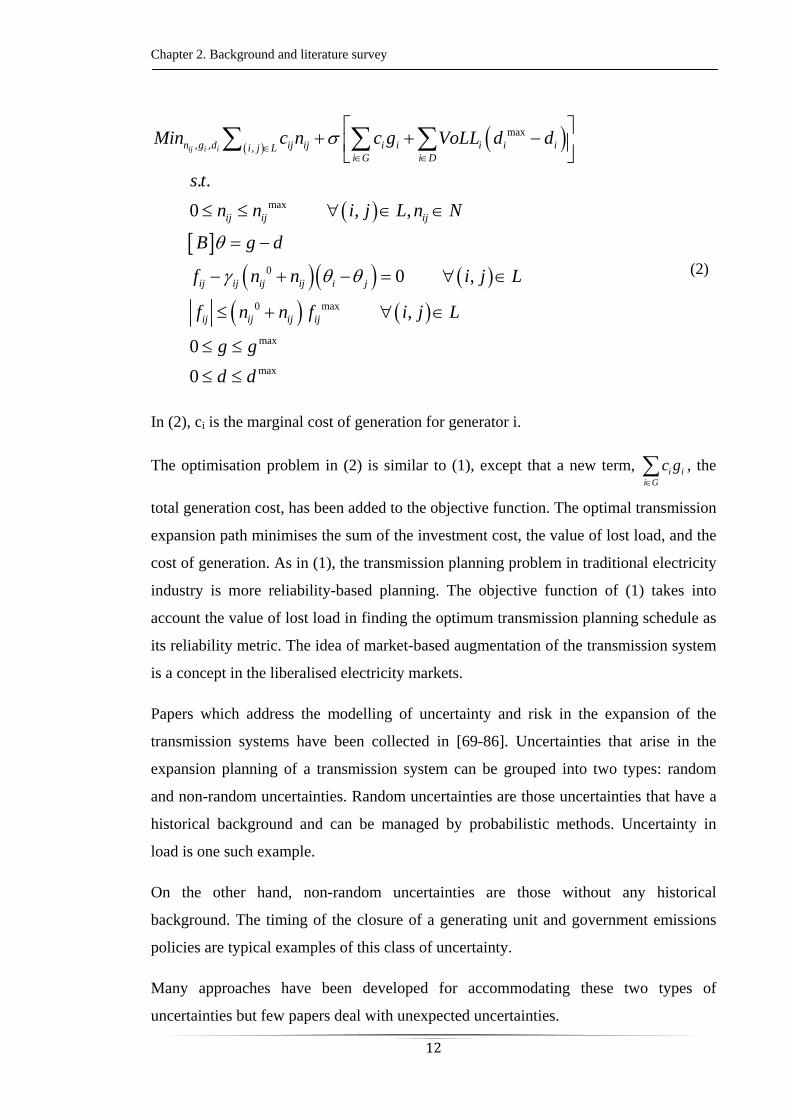
In (2), ci is the marginal cost of generation for generator i.
The optimisation problem in (2) is similar to (1), except that a new term, i ii G
c g , the
total generation cost, has been added to the objective function. The optimal transmission
expansion path minimises the sum of the investment cost, the value of lost load, and the
cost of generation. As in (1), the transmission planning problem in traditional electricity
industry is more reliability-based planning. The objective function of (1) takes into
account the value of lost load in finding the optimum transmission planning schedule as
its reliability metric. The idea of market-based augmentation of the transmission system
is a concept in the liberalised electricity markets.
Papers which address the modelling of uncertainty and risk in the expansion of the
transmission systems have been collected in [69-86]. Uncertainties that arise in the
expansion planning of a transmission system can be grouped into two types: random
and non-random uncertainties. Random uncertainties are those uncertainties that have a
historical background and can be managed by probabilistic methods. Uncertainty in
load is one such example.
On the other hand, non-random uncertainties are those without any historical
background. The timing of the closure of a generating unit and government emissions
policies are typical examples of this class of uncertainty.
Many approaches have been developed for accommodating these two types of
uncertainties but few papers deal with unexpected uncertainties.

Chapter 2. Background and literature survey
13
Market power of a producer is the ability to profitably maintain market prices above
competitive levels for a significant period of time, [87]. In economics, for a firm to have
market power, it is common said that two elements must be present:
First, the firm must have the ability to influence the market price by varying its
own output; and
Second, in doing so, the firm must be able to earn excess returns in the medium or
long-term, [88].
A firm which has no influence over the market price is said to be a price taker and is not
deemed to have market power.
The exercise of market power in electricity market involves reducing output in order to
raise the market price and thereby earn even higher overall profit on the remaining
output. This has two effects on prices:
The price-duration curve is higher than in the absence of market power;
The market price reaches the price cap more frequently and load shedding occurs
more frequently than in the absence of market power.
Reference [89] shows numerically that transmission expansion reduces generators’
market power. Reference [90] empirically examines the bidding behaviour of generators
in England and Wales, taking into account the impact of transmission constraints and
finds that generators protected by transmission constraints bid significantly higher than
those without this status.
There have been several occasions in the Australian National Electricity Market, NEM,
when a generator exercised market power because of constrained interconnectors. On 4
February 2003 an unplanned outage on the interconnector between the states of Victoria
and South Australia reduced its capacity substantially. Consequently, a large generator
in the South Australia region rebid 112MW of its capacity to prices greater than $9000,
[88].
Using a simplified version of the power network in California, reference [91] has
quantified the impact of local market power and transmission capacity. References [92]
and [93] show that generators benefit from a reduction in transmission capacity. Also,
Chapter 2. Background and literature survey
14
using a stylized version of the North America transmission system, reference [94]
highlights the effect of transmission capacity on encouraging competition among
Generating Companies, (GenCos).
Transmission capacity has been proven as an effective counter to market power, [95],
[96], [97]. Reference [98] suggests that policy makers can and should use transmission
capacity to reduce market power in electricity markets.
In reference [98] – a survey of publications on transmission expansion planning – no
technical literature is cited on the modelling of market power in the context of
transmission expansion planning.
Reference [96] sets up a framework for transmission planning based on the marginal
value of transmission capacity. Despite having a closed-form formulation, the
mechanism cannot model the effect of transmission capacity on market power.
Reference [99] employs the same mathematical structure as [96] but uses the congestion
cost and congestion revenue as the primary driving signals of the need for network
expansion. The lack of determination of the proper level of congestion for a
transmission network and the lack of modelling of the market power effect of additional
transmission capacity are the two main shortcomings of the proposed framework.
Reference [100] suggests two heuristic procedures for transmission augmentation. The
authors use an unconstrained oligopoly equilibrium for the set of producers’ bids while
the bids from the demand side are assumed as known from the analysis of the existing
market data. Clearly, an unconstrained oligopoly equilibrium cannot capture the effects
of transmission congestion in the electricity market.
The TEAM methodology introduced by the California ISO [101] is a good model for
economically-efficient transmission augmentation. However, it has two drawbacks.
Firstly, the strategic bidding of GenCos has been estimated through a tailor-made
empirical methodology which limits its application. Secondly, the whole framework
does not have an integrated mathematical structure.
To model the market power effect of transmission capacity in the process of
transmission augmentation, this research work proposes three closed-form constrained-
optimisation problems. These problems incorporate the modelling of strategic bidding
by generators using game theory concepts from applied mathematics.
Chapter 2. Background and literature survey
15
In the National Electricity Market, NEM, Australia, the “regulatory test” introduced by
the Australian Competition and Consumer Competition, ACCC, is used as criterion for
assessing proposed transmission augmentations by the transmission network service
providers over different states. In February 2003, the ACCC published a discussion
paper reviewing the regulatory test. Whether or not the “competition benefit” of
transmission capacity should be included in the regulatory test was one of the important
themes of the ACCC discussion report. “Competition benefit” is the additional market
benefit brought about by enhanced generator competition resulting from the
transmission augmentation.
Traditionally, modelling of transmission augmentations assumed a simplified form of
generator behaviour (such as assuming generators bid at marginal cost), ruling out
calculation of the impact of a transmission augmentation on competition between
generators. Reference [102], commissioned by the ACCC in June 2003, carried out a
review and analysis of the issues arising from the practical implementation of the
approaches to the measurement of competition benefits proposed by interested parties in
response to the Commission's discussion paper. Reference [103] has proposed a
heuristic approach for evaluating competition benefits of transmission capacity. The
integration of the competition benefit in the regulatory test is still under-developed and
demands more research. This is the primary objective of the remainder of this thesis.

CHAPTER 3 – A TECHNICAL INTRODUCTION TO THE
PROPOSED APPROACH
Chapter 3. A technical introduction …
17
3.1 Introduction
The objectives of this chapter are: (a) to test the concept of multi-level game
programming in assessing transmission investment decisions and (b) to study the impact
of additional transmission capacity on the behaviour of rival generating companies. The
chapter has its own technical notation and case study. This chapter can be considered as
an introduction to the approaches which are proposed and evaluated in the subsequent
chapters. However, the reader may wish to skip this chapter and start from chapter 4.
This chapter sets out a possible mathematical framework for modelling and assessing
expansions of the high voltage transmission system. The frame work uses a game
theoretic approach for modelling the “efficiency benefit” and the “competition benefit”
of additional transmission capacity. The economic value of a transmission augmentation
policy is measured through two indices: The first economic index is the notion of social
welfare. The social welfare of the liberalised electricity market is calculated assuming
that all GenCos offer their output at their true marginal cost to the Market Management
Company, MMC. The second index is the notion of monopoly rent. Rival GenCos are
assumed to play a Bertrand game. In the Nash equilibrium, of this Bertrand game the
monopoly rent is calculated as the excess profit each GenCo earns relative to the case of
competitive bidding. This index is assumed to be a measure of the level of market
power in the wholesale electricity market.
Section 3.2 sets out the mathematical derivation of the game-theoretic model. Section
3.3 proposes an iterative technique for solving the proposed game-theoretic framework.
Section 3.4 explores the application of the proposed framework for transmission
augmentation using a modified IEEE 14-bus example system. This chapter sets up and
examines concept that will be gradually improved in the following chapters of this
work.
3.2 The leader-follower model for transmission augmentation
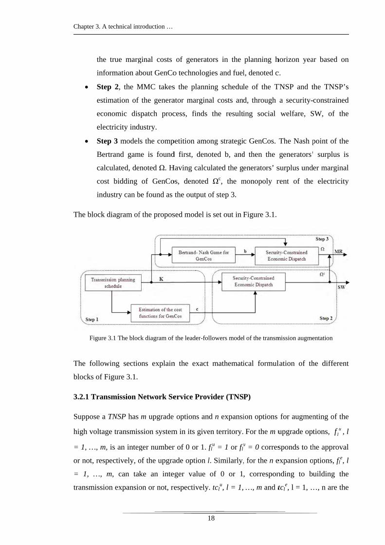
The leader-follower model of a transmission augmentation decision consists of three
steps or stages as presented in Figure 3.1:
Step 1, the TNSP determines the planning schedule of transmission system for
the horizon year. This planning schedule is denoted K. Also, the TNSP estimates
Chapter 3. A
the
inf
Ste
est
eco
ele
Ste
Be
cal
co
ind
The block
Figure
The follow
blocks of F
3.2.1 Tran
Suppose a
high volta
= 1, …, m
or not, res
= 1, …,
transmissi
A technical int
e true marg
formation ab
ep 2, the M
timation of
onomic dis
ectricity ind
ep 3 model
ertrand gam
lculated, de
st bidding
dustry can b
k diagram of
e 3.1 The bloc
wing sectio
Figure 3.1.
nsmission N
a TNSP has
age transmis
m, is an integ
spectively, o
m, can tak
ion expansio
troduction …
ginal costs
bout GenCo
MMC takes
f the genera
spatch proc
dustry.
ls the comp
me is found
enoted Ω. H
of GenCo
be found as
f the propos
ck diagram of
ons explain
Network Se
m upgrade
ssion system
ger number
of the upgra
ke an inte
on or not, re
1
of generat
o technolog
s the planni
ator margin
cess, finds
petition amo
d first, deno
Having calcu
os, denoted
the output o
sed model is
f the leader-fol
n the exact
ervice Prov
options an
m in its give
r of 0 or 1. f
ade option l
eger value
espectively
18
tors in the
gies and fuel
ing schedul
al costs and
the resulti
ong strategi
oted b, and
ulated the g
Ωc, the m
of step 3.
s set out in F
llowers model
mathemati
vider (TNS
d n expansi
en territory.
flu = 1 or fl
u
l. Similarly,
of 0 or 1
. tclu, l = 1,
planning h
l, denoted c
le of the T
d, through
ing social
c GenCos.
d then the
enerators’ s
monopoly r
Figure 3.1.
l of the transm
ical formul
P)
ion options
For the m u
u = 0 corres
, for the n e
, correspon
…, m and t
horizon yea
c.
TNSP and t
a security-
welfare, S
The Nash p
generators’
surplus und
rent of the
mission augme
lation of th
for augmen
upgrade opt
sponds to th
expansion o
nding to bu
tcle, l = 1, …
ar based on
the TNSP’s
constrained
SW, of the
point of the
surplus is
er marginal
electricity
entation
he different
nting of the
tions, ulf , l
he approval
ptions, fle, l
uilding the
…, n are the
n
s
d
e
e
s
l
y
t
e
l
l
l
e
e
Chapter 3. A technical introduction …
19
vectors of the investment cost for the transmission upgrade and expansion projects,
respectively.
The TNSP is assumed to seek to maximise the overall economic welfare less the
monopoly rent, less the cost of the upgrade or expansion. The monopoly rent metric,
MR, is used to model the competition benefit of additional transmission capacity.
Mathematically, the TNSP’s objective function can be formulated as (3.1).
,Π
. .
∈ 0,1 1, … ,
∈ 0,1 1, … , (3.1)
In (3.1), and are the TNSP’s design parameters. SW is the total surplus of the
electricity industry defined as the value of consumption to electricity consumers less the
variable cost of producing sufficient electricity to meet demand (3.2).
∑ . ∑ . (3.2)
In (3.2), is the value of lost load for each retailer, is the true marginal cost of
each GenCo. and are the GenCo j generation and the served demand of the
retailer i under marginal cost bidding scenario of GenCos. and are total number
of retailers and GenCos in the energy market.
is the weighting factor of the competition effect of transmission capacity. is set by
the electricity market regulator based on its judgement of the value of transmission
investment compared with the efficiency value and competition value of the
transmission capacity.
is the monopoly rent of the electricity industry defined as the excess profit over the
competitive bidding case, (3.3).
∑ Ω Ω , 0.0 (3.3)
Chapter 3. A technical introduction …
20
In (3.3), Ω is the profit of the ith GenCo under strategic bidding and Ω is the profit of
the same GenCo when it bids its true marginal cost. From the view point of economics a
firm has market power if it can change the price by changing its output and in doing so
earn extra profit. If the strategic bidding of a GenCo increases its profit, it will be taken
into account in the MR index, otherwise it will be set to zero.
3.2.2 Independent Generating Companies (GenCos)
Suppose a GenCo has a linear cost function of the form (3.4).
(3.4)
Where in (3.4), is the generation cost coefficient and is the generation output of
generator i. Considering (3.4), the GenCo objective function can be written as (3.5).
Ω (3.5)
Where in (3.5), is the price of electricity at the connection point of the ith GenCo.
is the by-product of the settlement process of the MMC.
Competition between generators can be modelled in different ways, corresponding to
different choices of the strategy space for each generator. Among the various choices,
the most common are the Bertrand game, Cournot game, and Supply Function
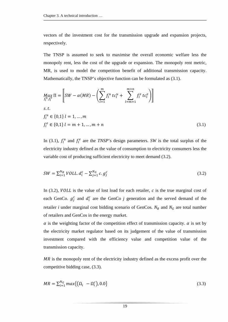
Equilibrium. This paper uses the Bertrand game in the modelling of competition among
GenCos. In the Bertrand game, each GenCo choices the price at which it offers its
output, assuming every other GenCo does the same. Each GenCo submits a bid pair of
, to the market with as the apparent marginal cost and as the
true maximum generation capacity of GenCo. Figure 3.2 shows the cost function of a
GenCo with and marked.
Chapter 3. A
Using the
the set of
strategy m
(3.6)
In (3.6),
bounded
maximum
limits
3.2.3 Mar
Following
electricity
and offers
market. Th
lost load f
economic
A technical int
Nash equi
strategies (
maximises it
Ω. .
is the Nash
by a lowe
m generation
and
rket Manag
g the approa
y market is
s and uses
he vectors
for the NR r
dispatch is
troduction …
librium con
(one for eac
ts profit give
⋯
h equilibriu
er and upp
n level of ea
.
gement Com
ach in the N
assumed to
a security
and
retailers. Th
set out in (3
C($
)
2
Figure 3.2 Ge
ncept, the e
ch GenCo)
en the strate
.
um of the G
per limit se
ach GenCo
mpany (MM
National El
o be a doub
y-constraine
are the stra
he mathema
3.7).
Cos
t ($)
21
enCo bid curv
equilibrium
where for e
egies of the
Ω. .
enCos, is
et by the m
, , is
MC)
lectricity M
le-sided gro
ed economi
ategic bids
atical formu
ve
point of th
each genera
other gener
⋯
s the strateg
market reg
bounded by
Market in Au
oss pool. Th
ic dispatch
of NG gener
ulation of th
Quan
he electricity
ator, the cor
rators, (3.6
Ω.
gic bidding
gulator. Sim
y the upper
ustralia, the
he MMC c
h process to
rators and t
he security-
ntity (MW)
y market is
rresponding
6).
.
factor. is
milarly, the
r and lower
e wholesale
ollects bids
o clear the
the value of
constrained
s
g
s
e
r
e
s
e
f
d
Chapter 3. A technical introduction …
22
, , . .
. .
(3.7)
In (3.7), and are 1 and 1 matrices where the column
related to the slack bus is omitted, and are the total number of buses and total
number of lines in the system. is the vector of bus angles, and are the generation
level of committed generators and the served demand of retailers. , , and are the
decision variable of (3.7). These variables are bounded by their minimum and
maximum values. The existing capacity of the transmission system has been modelled
through the vector .
3.3 An iterative process for TNSP’s decision making
The TNSP uses an iterative process for designing the future transmission system. In this
process, the security-constrained economic dispatch of the MMC, set out in equation
3.7, is solved using the revised simplex method. The equilibrium of the strategic
behaviour of the GenCos, as set out in equation set 3.6, is found using a non-linear
Gauss-Seidel method, as explained in section 3.3.1. Finally, the TNSP uses the heuristic
method described in 3.3.2 for the final design of the high voltage transmission lines.
3.3.1 The Non-Linear Gauss-Seidel Method for finding the equilibrium of the
Bertrand-Nash Game of GenCos using an embedded bilevel formulation of the
profit maximisation of a GenCo
Chapter 3. A technical introduction …
23
Ω. .
⋯
Ω. .
⋯
Ω. .
, , . .. .
(3.8)
The programming problem (3.8) can be categorised as a non-linear bilevel programming
problem. Generally, non-linear bilevel programming programs are intrinsically hard.
The proposed numerical method for solving (3.8) is as follows.
In equation (3.8), each GenCo solves a Mathematical Programming with Equilibrium
Constraints, MPEC, which represents the profit maximisation of the GenCo. In this
level, each GenCo maximises its own revenue taking as given the bidding of the other
GenCos.
The MMC’s central dispatch process can be written as in (3.9).
.
. .
(3.9)
Vectors and matrices in (3.9) are defined in terms of the vectors and matrices in (3.8) as
follows;
Chapter 3. A technical introduction …
24
and are the matrices which determine the transmission connection buses of the
registered generators and retailers in the electricity market.
Writing the Kuhn-Tucker (KT) optimality conditions for (3.9), simplifying and
differentiating the KT optimality conditions with respect to , yields the following sets
of equations.
0 (3.10)
Where in (3.10), is the vector of slack variables. Using the transpose properties of
and , equation set (3.10) can be
written in the following matrix form;
Chapter 3. A technical introduction …
25
(3.11)
In (3.11), vector reflects the gradient components of the ith GenCo
objective function, Ω . In some cases, the rank of the left hand side matrix in (3.11) is
lower than the number of variables in (3.11). In these cases, a singular value
decomposition methodology has been employed as one of the best methods for solving
least-squares problems. When the (3.11) have multiple solutions, it means there are
different convergence patterns to the optimal solution of the problem. At the end, all of
these patterns should converge to the same optimal answer.
The partial derivative of the Ω with respect to the can be found as in (3.12).
(3.12)
Using the gradient search technique, the algorithm starts with an initial guess for , and
updates the value of based on equation (3.13).
(3.13)
Where is the step length of the movement towards the new solution. To protect the
algorithm against non differentiable points, in each iteration of , the algorithm checks
the variables of the (3.11) to determine if they have reached their upper or lower limits.
In either case, the algorithm gets back to the previous value of and terminates the
iteration.
To locate the globally optimal bidding strategy for each GenCo, the bidding space has
been divided into several segments. The optimal bid on each segment is calculated and
saved using the gradient method explained above. The best bid of these segments is
selected as the best bidding strategy of the GenCo. Proper division of the bidding space
is very important in locating the global optimum of the GenCo optimisation problem.

Chapter 3. A technical introduction …
26
The division of the bidding space into segments is experimental. I tried different values
for dividing the bidding space and then the best one was selected. However, this cannot
guarantee the best solution.
Equation set (3.8) is an Equilibrium Problem with Equilibrium Constraints (EPEC)
which finds the Nash equilibrium point of the GenCos. By the definition of a Nash
equilibrium, no GenCo can increase its profit by unilaterally deviating from the
equilibrium, i.e.,
∗ ∀ , ∗ ∈ arg Ω | ∗ (3.14)
Where in (3.14), ∗ is the vector of optimal strategies of the other GenCos.
A diagonalization method and a sequential nonlinear complementarity algorithm are
used for solving the Nash equilibrium problem. Nonlinear Jacobi and nonlinear Gauss-
Seidel are two diagonalization methods.
Nonlinear Gauss-Seidel is used for the solution of (3.8) and is described as follows:
Step 1. Initialization.
Choose a starting point for each GenCo, the maximum number of Gauss-Seidel
iterations L, and an accuracy tolerance 0.0 .
Step 2. Loop over every MPEC (The individual GenCo’s optimisation problem in (3.8)).
Suppose the current iteration point of is . For each GenCo i, the MPEC is solved
while fixing , … , , , … ,
Step 3. Check convergence.
If , then increase l by one and repeat step 1. Otherwise, stop and check the
accuracy tolerance. If ∥ ∥ for all GenCos, then accept and report the
solution; otherwise, output “No equilibrium point found”.
If the problem has no Nash equilibrium, the Gauss-Seidel algorithm will not converge.
However, the algorithm will find one equilibrium point as long as a Nash equilibrium of
the problem exists. Also, it should be noted that in some cases the Gauss-Seidel method
cannot find the Nash equilibrium of the game.
Chapter 3. A technical introduction …
27
Once the Nash equilibrium with strategic bidding behaviour of GenCos is found, the
system monopoly rent, MR, can be calculated by finding the difference between the
GenCos’ profit in the two scenarios of (a) bidding strategically and (b) bidding at true
marginal cost.
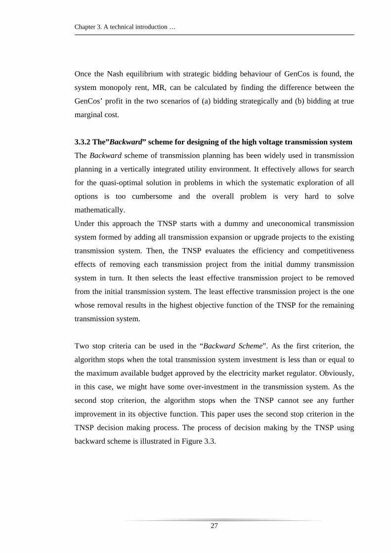
3.3.2 The”Backward” scheme for designing of the high voltage transmission system
The Backward scheme of transmission planning has been widely used in transmission
planning in a vertically integrated utility environment. It effectively allows for search
for the quasi-optimal solution in problems in which the systematic exploration of all
options is too cumbersome and the overall problem is very hard to solve
mathematically.
Under this approach the TNSP starts with a dummy and uneconomical transmission
system formed by adding all transmission expansion or upgrade projects to the existing
transmission system. Then, the TNSP evaluates the efficiency and competitiveness
effects of removing each transmission project from the initial dummy transmission
system in turn. It then selects the least effective transmission project to be removed
from the initial transmission system. The least effective transmission project is the one
whose removal results in the highest objective function of the TNSP for the remaining
transmission system.
Two stop criteria can be used in the “Backward Scheme”. As the first criterion, the
algorithm stops when the total transmission system investment is less than or equal to
the maximum available budget approved by the electricity market regulator. Obviously,
in this case, we might have some over-investment in the transmission system. As the
second stop criterion, the algorithm stops when the TNSP cannot see any further
improvement in its objective function. This paper uses the second stop criterion in the
TNSP decision making process. The process of decision making by the TNSP using
backward scheme is illustrated in Figure 3.3.
Chapter 3. A
Section 3.
example s
A technical int
Figure 3.3 Th
.4 deals wi
system.
troduction …
he decision ma
ith applicati
2
making process
ion of this
28
s of the TNSP
methodolo
using the bac
gy to the m
ckward schem
modified IE
me
EEE 14-bus
s
Chapter 3. A
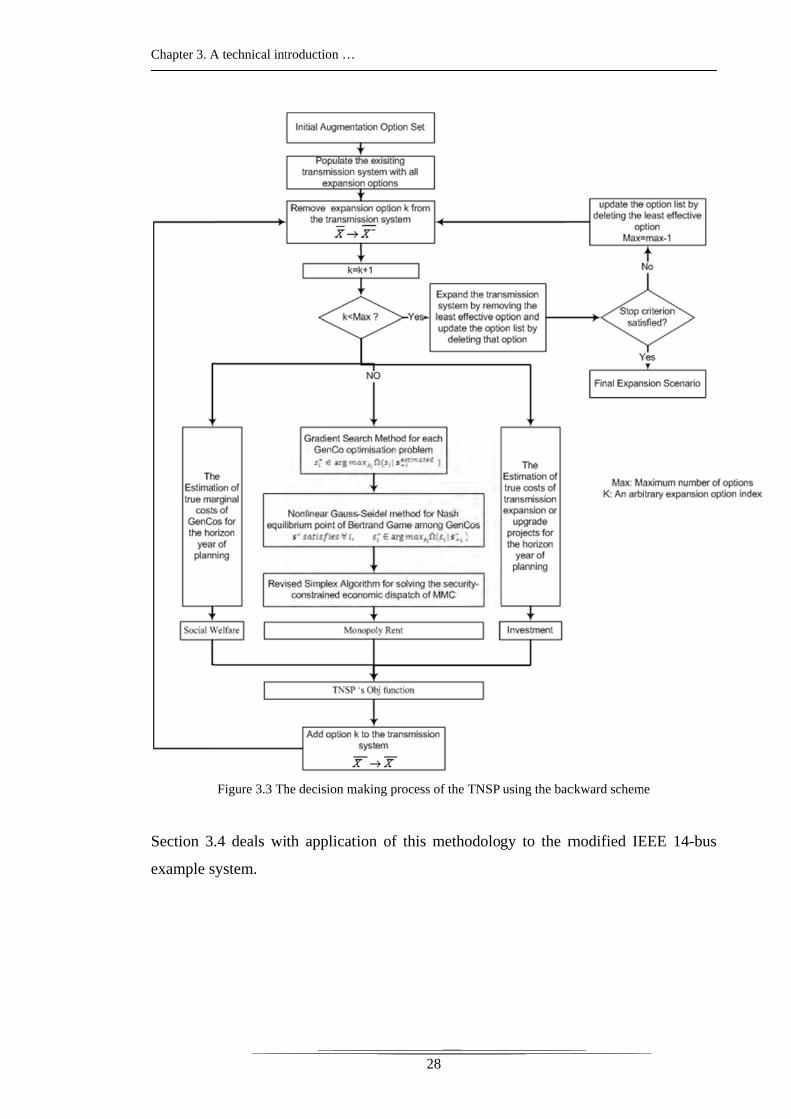
3.4 Applic
The modi
show the e
There are
labelled R
augmentat
the existin
Tables 3.1
for the exi
A technical int
cation to th
fied IEEE
effectivenes
five strateg
R1 to R11
tion of the
ng transmis
1, 3.2, 3.3,
isting transm
troduction …
he modified
14-bus test
ss of the pro
Figure 3.4
gic generat
in the 14-b
transmissio
sion netwo
and 3.4 res
mission syst
2
d IEEE 14-
t system de
oposed algo
The modified
tors labelled
bus exampl
on system. K
ork, and the
spectively. T
tem are coll
29
bus examp
epicted in F
orithm.
d IEEE 14-bus
d G1 to G5
le system. T
Key inform
e potential t
The potenti
lected in Ta
ple system
Figure 3.4 h
s test system
5, and eleve
The TNSP
mation on th
transmission
ial upgrade
able 3.4.
has been em
en competi
is responsi
he generator
n projects i
or expansi
mployed to
ng retailers
ible for the
rs, retailers,
is shown in
ion projects
o
s
e
,
n
s

Chapter 3. A technical introduction …
30
Table 3.1 Generators’ data
Generator (MW) (MW) ($/MWh)
G1 0.0 132 38.2
G2 0.0 180 25.2
G3 0.0 120 16.7
G4 0.0 170 43.5
G5 0.0 140 12.7
Total 0.0 742
Table 3.2 Retailers’ data
Retailer (MW) (MW) ($/MWh)
R1 0.0 41.7 151
R2 0.0 184.2 177
R3 0.0 87.8 154
R4 0.0 34.6 157
R5 0.0 21.2 153
R6 0.0 89.5 165
R7 0.0 29 169
R8 0.0 136.5 153
R9 0.0 12.1 166
R10 0.0 26.2 156
R11 0.0 48.9 158
Total Demand 0.0 711.7
Table 3.3 Transmission network data
Line# From To Reactance (p.u.) Limit (MW)
1 B1 B2 0.05917 70
2 B1 B5 0.22304 70
3 B2 B3 0.19797 70
4 B2 B4 0.17632 70
5 B2 B5 0.17388 70
6 B3 B4 0.17103 70
7 B4 B5 0.04211 70
8 B4 B7 0.20912 70
9 B4 B9 0.55618 70
10 B5 B6 0.25202 70
11 B6 B11 0.19890 70
12 B6 B12 0.25581 70
Chapter 3. A technical introduction …
31
13 B6 B13 0.13027 70
14 B7 B8 0.17615 70
15 B7 B9 0.11001 70
16 B9 B10 0.08450 70
17 B9 B14 0.27038 70
18 B10 B11 0.19207 70
19 B12 B13 0.19988 70
20 B13 B14 0.34802 70
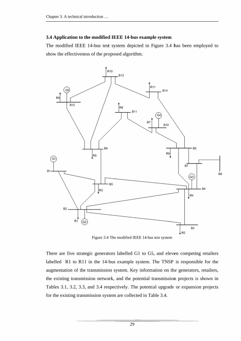
Table 3.4 Transmission network upgrade or expansion data
Project # From To Reactance (p.u.) Limit (MW) Investment cost ($)
1 B1 B2 0.0592 100 5100
2 B1 B5 0.2230 100 4500
3 B1 B12 0.0180 100 2500
4 B1 B6 0.0170 100 1500
5 B1 B9 0.0160 100 2500
6 B1 B11 0.0150 100 3500
7 B2 B3 0.1980 100 2200
8 B2 B4 0.1763 100 1700
9 B2 B5 0.1739 100 1900
10 B2 B13 0.1150 100 3700
11 B2 B14 0.1610 100 2700
12 B3 B4 0.1710 100 4200
13 B3 B12 0.1300 100 3200
14 B3 B10 0.1410 100 2900
15 B4 B11 0.0200 100 1200
16 B4 B6 0.1700 100 1800
17 B4 B14 0.1100 100 4500
18 B5 B10 0.0500 100 2300
19 B9 B2 0.0800 100 4900
20 B10 B3 0.0200 100 2100
21 B10 B14 0.1500 100 3600
22 B10 B13 0.0300 100 1400
23 B11 B12 0.2300 100 1800
24 B12 B13 0.1900 100 3500
25 B13 B14 0.2200 100 330
26 B6 B12 0.2300 100 1100
27 B1 B2 0.0500 100 4800
28 B2 B3 0.1900 100 2000
Chapter 3. A technical introduction …
32
29 B3 B4 0.1700 100 4000
30 B6 B12 0.2300 100 1000
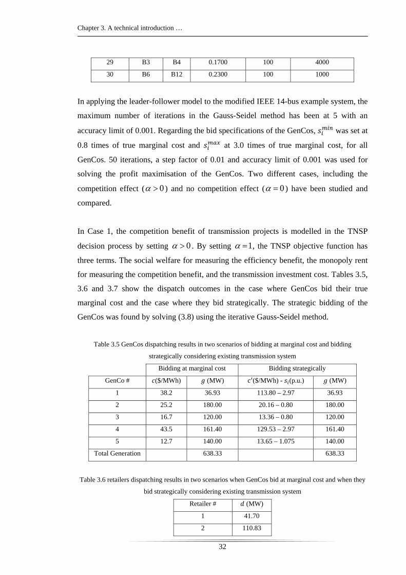
In applying the leader-follower model to the modified IEEE 14-bus example system, the
maximum number of iterations in the Gauss-Seidel method has been at 5 with an
accuracy limit of 0.001. Regarding the bid specifications of the GenCos, was set at
0.8 times of true marginal cost and at 3.0 times of true marginal cost, for all
GenCos. 50 iterations, a step factor of 0.01 and accuracy limit of 0.001 was used for
solving the profit maximisation of the GenCos. Two different cases, including the
competition effect ( 0 ) and no competition effect ( 0 ) have been studied and
compared.
In Case 1, the competition benefit of transmission projects is modelled in the TNSP
decision process by setting 0 . By setting 1 , the TNSP objective function has
three terms. The social welfare for measuring the efficiency benefit, the monopoly rent
for measuring the competition benefit, and the transmission investment cost. Tables 3.5,
3.6 and 3.7 show the dispatch outcomes in the case where GenCos bid their true
marginal cost and the case where they bid strategically. The strategic bidding of the
GenCos was found by solving (3.8) using the iterative Gauss-Seidel method.
Table 3.5 GenCos dispatching results in two scenarios of bidding at marginal cost and bidding
strategically considering existing transmission system
Bidding at marginal cost Bidding strategically
GenCo # ($/MWh) (MW) c ($/MWh) - (p.u.) (MW)
1 38.2 36.93 113.80 – 2.97 36.93
2 25.2 180.00 20.16 – 0.80 180.00
3 16.7 120.00 13.36 – 0.80 120.00
4 43.5 161.40 129.53 – 2.97 161.40
5 12.7 140.00 13.65 – 1.075 140.00
Total Generation 638.33 638.33
Table 3.6 retailers dispatching results in two scenarios when GenCos bid at marginal cost and when they
bid strategically considering existing transmission system
Retailer # (MW)
1 41.70
2 110.83

Chapter 3. A technical introduction …
33
3 87.80
4 34.60
5 21.20
6 89.50
7 29.00
8 136.50
9 12.10
10 26.20
11 48.90
Total Demand 638.33
Table 3.7 transmission lines flows in MW for two scenarios when GenCos bid at marginal cost and when
they bid strategically considering existing transmission system
From To MW flow Shadow price of transmission line ($/MWh)
Bidding at marginal cost Bidding strategically
B1 B2 6.89 0 0
B1 B5 30.04 0 0
B2 B3 70.00Congested -2.63 -1.19
B2 B4 38.99 0 0
B2 B5 36.19 0 0
B3 B4 -40.83 0 0
B4 B5 -13.82 0 0
B4 B7 28.08 0 0
B4 B9 16.11 0 0
B5 B6 17.81 0 0
B6 B11 66.50 0 0
B6 B12 -59.17 0 0
B6 B13 -10.72 0 0
B7 B8 0 0 0
B7 B9 28.08 0 0
B9 B10 -62.40 0.0 0
B9 B14 17.09 0 0
B10 B11 70.00 Congested -1.06 -0.01
B12 B13 68.73 0 0
B13 B14 31.81 0 0
As Table 3.7 shows, the shadow prices of the transmission lines are completely different
in the two scenarios of bidding at marginal cost and bidding strategically. Figure 3.5

Chapter 3. A technical introduction …
34
shows the price of electricity at each bus in the two scenarios of strategic bidding and
marginal cost bidding of GenCos.
Figure 3.5 Price profile of the modified IEEE 14-bus example system for two scenarios of bidding at
marginal cost and bidding strategically considering the existing transmission system in horizon year of
planning
As is clear from Figure 3.5, considering the existing transmission system for the horizon
year of planning, the effect of strategic bidding is to increase the average energy price
from 76.49 $/MWh to 130.27 $/MWh. The total surplus of the system when GenCos bid
at marginal cost is $85735.44 while for the strategic bidding scenario, the total surplus
has dropped by 18.08% to $70233.65. In this case, the monopoly rent, MR, of GenCos
1, 2, 3, 4, 5, and total monopoly rent are $2792, $14370, $6670, $13885, $5561, and
$43279, respectively.
The above analysis of the existing transmission system for the horizon year suggests the
TNSP needs to augment the transmission system to improve the total surplus of the
system and also to encourage competition among GenCos.
Bidding strategically (price average 130.27$/MWh)
Bidding at marginal cost (price average 76.49$/MWh)
Bus
Price($/M
Wh)
Chapter 3. A technical introduction …
35
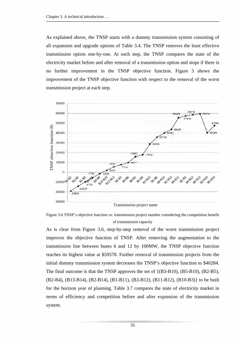
As explained above, the TNSP starts with a dummy transmission system consisting of
all expansion and upgrade options of Table 3.4. The TNSP removes the least effective
transmission option one-by-one. At each step, the TNSP compares the state of the
electricity market before and after removal of a transmission option and stops if there is
no further improvement in the TNSP objective function. Figure 5 shows the
improvement of the TNSP objective function with respect to the removal of the worst
transmission project at each step.
Figure 3.6 TNSP’s objective function vs. transmission project number considering the competition benefit
of transmission capacity
As is clear from Figure 3.6, step-by-step removal of the worst transmission project
improves the objective function of TNSP. After removing the augmentation to the
transmission line between buses 6 and 12 by 100MW, the TNSP objective function
reaches its highest value at $59578. Further removal of transmission projects from the
initial dummy transmission system decreases the TNSP’s objective function to $40284.
The final outcome is that the TNSP approves the set of (B3-B10), (B5-B10), (B2-B5),
(B2-B4), (B13-B14), (B2-B14), (B1-B11), (B3-B12), (B11-B12), (B10-B3) to be built
for the horizon year of planning. Table 3.7 compares the state of electricity market in
terms of efficiency and competition before and after expansion of the transmission
system.
TN
SP
obje
ctiv
efu
nctio
n($
)
Transmission project name
Chapter 3. A technical introduction …
36
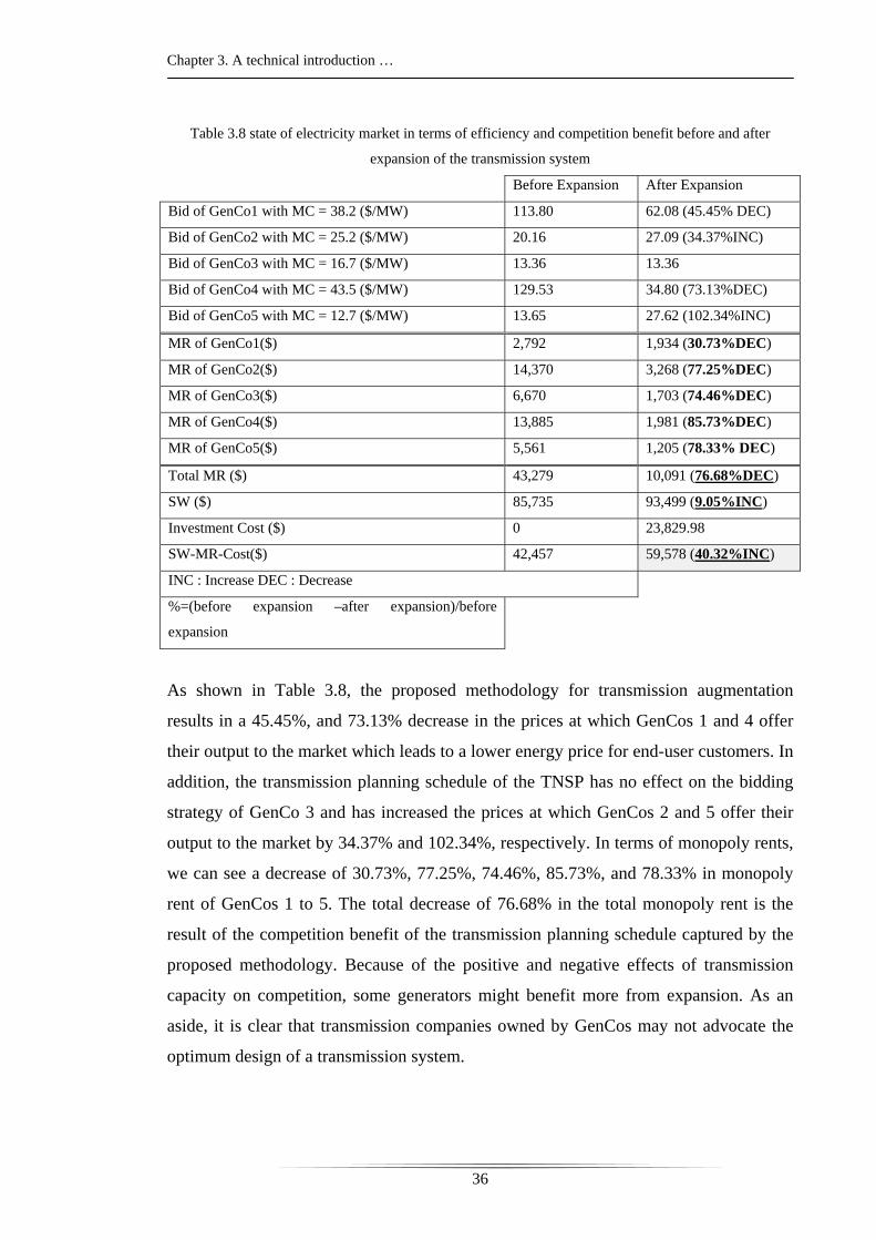
Table 3.8 state of electricity market in terms of efficiency and competition benefit before and after
expansion of the transmission system
Before Expansion After Expansion
Bid of GenCo1 with MC = 38.2 ($/MW) 113.80 62.08 (45.45% DEC)
Bid of GenCo2 with MC = 25.2 ($/MW) 20.16 27.09 (34.37%INC)
Bid of GenCo3 with MC = 16.7 ($/MW) 13.36 13.36
Bid of GenCo4 with MC = 43.5 ($/MW) 129.53 34.80 (73.13%DEC)
Bid of GenCo5 with MC = 12.7 ($/MW) 13.65 27.62 (102.34%INC)
MR of GenCo1($) 2,792 1,934 (30.73%DEC)
MR of GenCo2($) 14,370 3,268 (77.25%DEC)
MR of GenCo3($) 6,670 1,703 (74.46%DEC)
MR of GenCo4($) 13,885 1,981 (85.73%DEC)
MR of GenCo5($) 5,561 1,205 (78.33% DEC)
Total MR ($) 43,279 10,091 (76.68%DEC)
SW ($) 85,735 93,499 (9.05%INC)
Investment Cost ($) 0 23,829.98
SW-MR-Cost($) 42,457 59,578 (40.32%INC)
INC : Increase DEC : Decrease
%=(before expansion –after expansion)/before
expansion
As shown in Table 3.8, the proposed methodology for transmission augmentation
results in a 45.45%, and 73.13% decrease in the prices at which GenCos 1 and 4 offer
their output to the market which leads to a lower energy price for end-user customers. In
addition, the transmission planning schedule of the TNSP has no effect on the bidding
strategy of GenCo 3 and has increased the prices at which GenCos 2 and 5 offer their
output to the market by 34.37% and 102.34%, respectively. In terms of monopoly rents,
we can see a decrease of 30.73%, 77.25%, 74.46%, 85.73%, and 78.33% in monopoly
rent of GenCos 1 to 5. The total decrease of 76.68% in the total monopoly rent is the
result of the competition benefit of the transmission planning schedule captured by the
proposed methodology. Because of the positive and negative effects of transmission
capacity on competition, some generators might benefit more from expansion. As an
aside, it is clear that transmission companies owned by GenCos may not advocate the
optimum design of a transmission system.
Chapter 3. A technical introduction …
37
Overal, the proposed planning schedule of the TNSP encourages competition among
GenCos to the extent that the monopoly rent (MR) reduces by 76.68%, and improves
the overall social welfare of the energy market by 9.05%. Taking into account the
investment cost of transmission augmentation, the total improvement in the TNSP’s
objective function from the expansion is calculated as 40.32%.
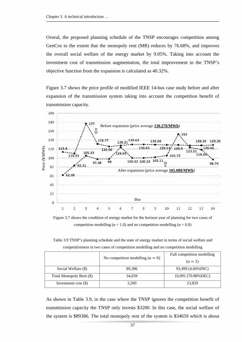
Figure 3.7 shows the price profile of modified IEEE 14-bus case study before and after
expansion of the transmission system taking into account the competition benefit of
transmission capacity.
Figure 7 Price profile of the modified IEEE 14-bus example system before and after expansion of
transmission system with competition benefit modelling
Figure 3.7 shows the condition of energy market for the horizon year of planning for two cases of
competition modelling (α = 1.0) and no competition modelling (α = 0.0)
Table 3.9 TNSP’s planning schedule and the state of energy market in terms of social welfare and
competitiveness in two cases of competition modelling and no competition modelling
No competition modelling (α 0) Full competition modelling
(α 1)
Social Welfare ($) 89,386 93,499 (4.60%INC)
Total Monopoly Rent ($) 34,659 10,091 (70.88%DEC)
Investment cost ($) 3,200 23,829
As shown in Table 3.9, in the case where the TNSP ignores the competition benefit of
transmission capacity the TNSP only invests $3200. In this case, the social welfare of
the system is $89386. The total monopoly rent of the system is $34659 which is about
Pri
ce (
$/M
Wh)
Bus
Before expansion (price average 130.27$/MWh)
After expansion (price average 105.08$/MWh)
Chapter 3. A technical introduction …
38
one third of system social welfare. On the other hand, when modelling competition
through the proposed methodology, the TNSP invests $23829. The social welfare of the
system is increased to $93499 and the monopoly rent is reduced to $10091. The new
investment strategy leads to a rise of 4.60% in social welfare and 70.88% increase in the
competitiveness of electricity market.
I conclude that a TNSP, in designing the transmission system must look beyond social
welfare improvement alone and, in particular, must take into account the scope for
increasing competition among GenCos.
3.5 Conclusion
This paper presents a leader-follower model for modelling of the process of choosing an
optimal set of transmission augmentations. The proposed model can design the horizon
year transmission system taking into account both the efficiency and competitiveness of
the electricity market. Using the Nash equilibrium concept, the TNSP evaluates
transmission projects taking into account all possible responses from the GenCos and
the decisions of the MMC. Security-constrained economic dispatch used by the MMC is
modelled as a linear programming problem solved by the revised simplex method. The
profit maximisation problem of each GenCo is modelled as a bilevel programming
problem. A gradient search method using the Kuhn-Tucker optimality conditions is
employed to solve each GenCo’s optimisation problem. The Nash equilibrium point is
found using the iterative Gauss-Seidel method. Finally, the TNSP uses a step-by-step
removal methodology for evaluating transmission projects. The numerical results show
that (1) transmission capacity has obvious effects on both efficiency and
competitiveness of electricity markets (2) expansion of one transmission corridor can
increase or decrease market power and consequently can have negative and positive
competitiveness effect (3) TNSPs owned and operated by GenCos may not advocate
optimal transmission expansion (4) considering the strategic behaviour of GenCos,
congestion-driven transmission expansion does not lead to efficient transmission
expansion decisions and (5) policy makers and TNSPs must expand the transmission
system beyond that suggested by a social welfare criterion alone. The proposed
methodology can effectively model the optimisation problem faced by the TNSP,
GenCos, and the MMC in an integrated mathematical framework. In addition, it can
design the horizon year transmission system by capturing the efficiency effect and
competition effect of additional transmission capacity.
CHAPTER 4 – DIFFERENT APPROACHES TO THE
ASSESSMENT OF TRANSMISSION AUGMENTATION
POLICIES
Chapter 4. Different approaches to …
40
4.1 Introduction
This chapter sets out four different possible approaches for the assessment of
augmentations of the transmission system. These approaches differ primarily in the
objective function of the system operator. The first approach uses, as the objective
function, a new metric called here the L-Shape Area metric. The second approach uses,
as the objective function of the system operator, the concept of monopoly rent. The
third approach uses the economic concept of social welfare. The fourth approach differs
from the others in that it models the potential for strategic generation investment.
This chapter is organised as follows. Section 4.2 explores the assessment of a
transmission augmentation approach using the L-Shape area metric. The use of the
concept of monopoly rent as the objective of the system operator is covered in section
4.3. The use of the concept of social welfare is discussed in section 4.4. Finally, the
modelling of strategic generation investment is discussed in section 4.5..
4.2. The developed L-Shape area metric
This section focuses on modelling the behaviour of the following participants in the
electricity market:
The Generating Companies, GenCos, which are assumed to be private, profit-
maximising entities which compete with each other in the strategic game set out
below.
The Transmission Network Service Provider, TNSP, who is responsible for the
operation of and investment in the shared transmission system. The TNSP is
assumed to be a regulated monopoly business.
Retailers, who buy electrical energy from the GenCos and deliver it to end user
customers; and
The Electricity Market Operator, EMO, which manages and operates the
electricity market. We disregard the possibility of strategic behaviour of the
retailers.
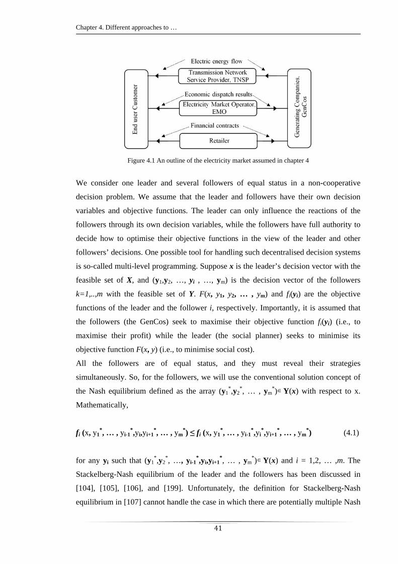
The electricity market architecture assumed in this chapter is illustrated in Figure 4.1.
Chapter 4. Different approaches to …
41
Figure 4.1 An outline of the electricity market assumed in chapter 4
We consider one leader and several followers of equal status in a non-cooperative
decision problem. We assume that the leader and followers have their own decision
variables and objective functions. The leader can only influence the reactions of the
followers through its own decision variables, while the followers have full authority to
decide how to optimise their objective functions in the view of the leader and other
followers’ decisions. One possible tool for handling such decentralised decision systems
is so-called multi-level programming. Suppose x is the leader’s decision vector with the
feasible set of X, and (y1,y2, …, yi , …, ym) is the decision vector of the followers
k=1,..,m with the feasible set of Y. F(x, y1, y2, … , ym) and fi(yi) are the objective
functions of the leader and the follower i, respectively. Importantly, it is assumed that
the followers (the GenCos) seek to maximise their objective function fi(yi) (i.e., to
maximise their profit) while the leader (the social planner) seeks to minimise its
objective function F(x, y) (i.e., to minimise social cost).
All the followers are of equal status, and they must reveal their strategies
simultaneously. So, for the followers, we will use the conventional solution concept of
the Nash equilibrium defined as the array (y1*,y2
*, … , ym*)Y(x) with respect to x.
Mathematically,
fi (x, y1*, … , yi-1
*,yi,yi+1*, … , ym
*) ≤ fi (x, y1*, … , yi-1
*,yi*,yi+1
*, … , ym*) (4.1)
for any yi such that (y1*,y2
*, …, yi-1*,yi,yi+1
*, … , ym*)Y(x) and i = 1,2, … ,m. The
Stackelberg-Nash equilibrium of the leader and the followers has been discussed in
[104], [105], [106], and [199]. Unfortunately, the definition for Stackelberg-Nash
equilibrium in [107] cannot handle the case in which there are potentially multiple Nash
Chapter 4. Different approaches to …
42
equilibria for any given leader’s action. To solve this problem, we propose the
Stackelberg-Worst Nash equilibrium as in Definition 1.
Definition 1: Stackelberg-Worst Nash Equilibrium
Let Y*(x) be the set of all Nash equilibria with respect to leader’s action xX. (y1*,y2
*,
… , ym*) Y*(x) is said to be the worst Nash equilibrium for action x if and only if
(x, y1*,y2
*, … , ym*) arg Max F(x, y1,y2, … , ym) (4.2)
where (y1,y2, … , ym) Y*(x).
Also, (x*, y1*,y2
*, … , ym*) is said to be the Stackelberg-Worst Nash equilibrium of the
leader and the followers if and only if
(x*, y1*, y2
*, … , ym*) arg Min F(x, y1,y2, … , ym) (4.3)
where xX and (y1,y2, … , ym) is the worst Nash equilibrium for action x.
The proposed methodology for transmission planning is developed in three steps. Step 1
models the strategic behaviour of a GenCo in an oligopoly framework. In step 2, the
Nash solution concept is reformulated as an optimisation problem. Step 3 employs the
concept of the Stackelberg-Worst Nash equilibrium and the concept of social welfare in
economics to derive the decision problem of the social planner. In what follows, we
explain these steps in detail.
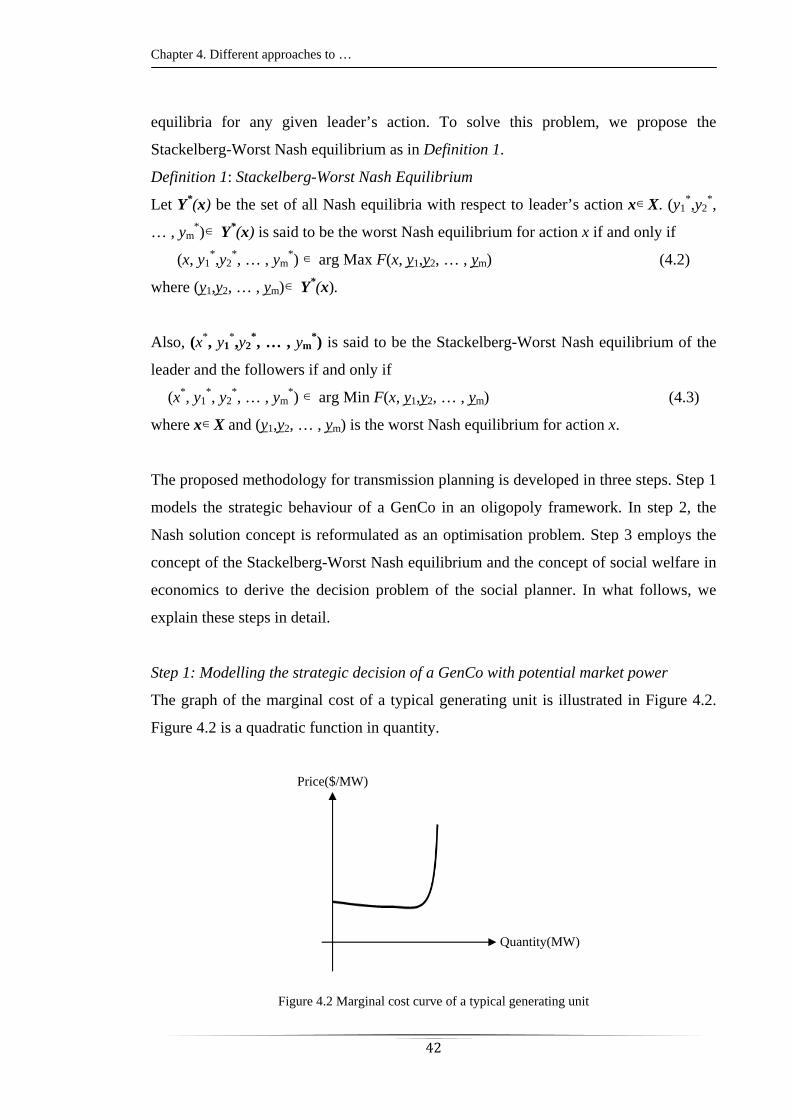
Step 1: Modelling the strategic decision of a GenCo with potential market power
The graph of the marginal cost of a typical generating unit is illustrated in Figure 4.2.
Figure 4.2 is a quadratic function in quantity.
Figure 4.2 Marginal cost curve of a typical generating unit
Quantity(MW)
Price($/MW)
Chapter 4. Different approaches to …
43
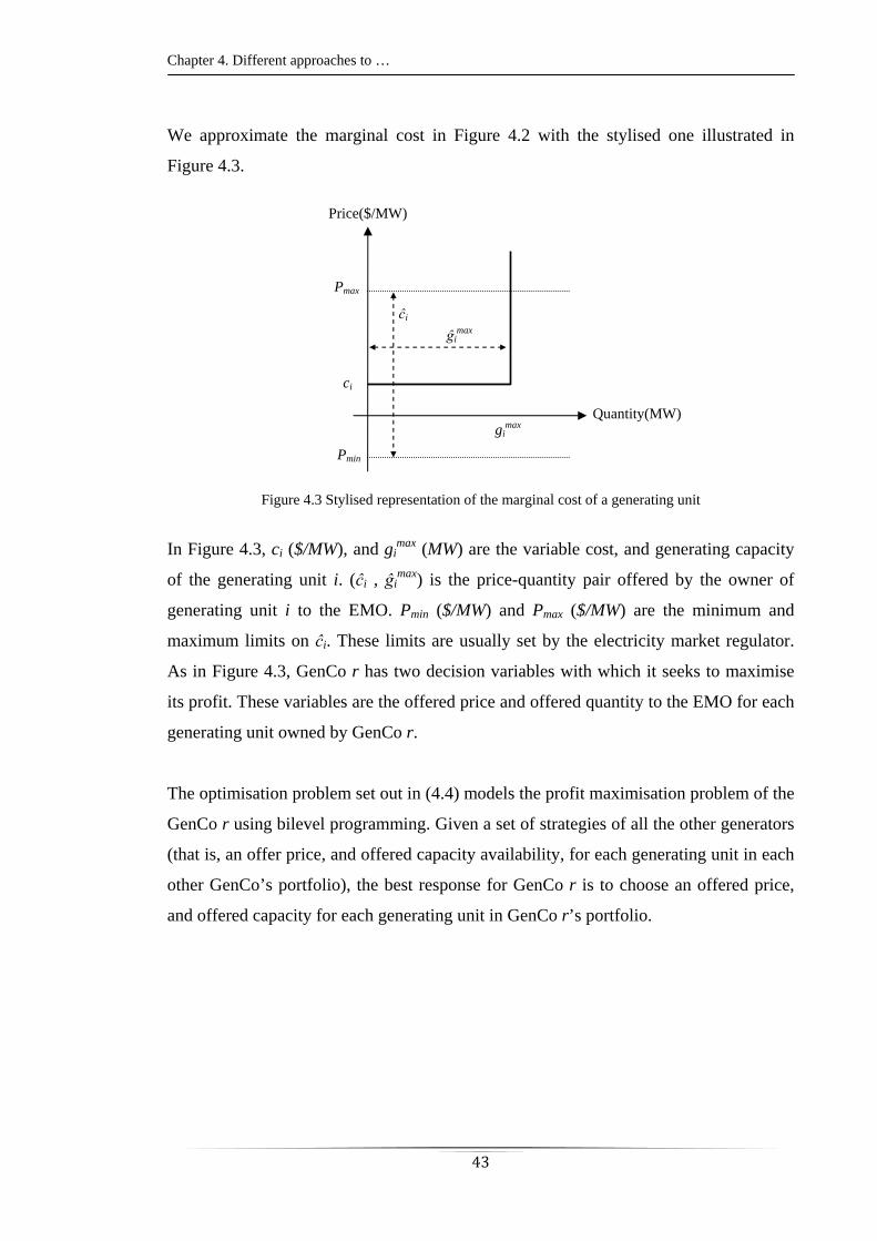
We approximate the marginal cost in Figure 4.2 with the stylised one illustrated in
Figure 4.3.
Figure 4.3 Stylised representation of the marginal cost of a generating unit
In Figure 4.3, ci ($/MW), and gimax (MW) are the variable cost, and generating capacity
of the generating unit i. (ĉi , ĝimax) is the price-quantity pair offered by the owner of
generating unit i to the EMO. Pmin ($/MW) and Pmax ($/MW) are the minimum and
maximum limits on ĉi. These limits are usually set by the electricity market regulator.
As in Figure 4.3, GenCo r has two decision variables with which it seeks to maximise
its profit. These variables are the offered price and offered quantity to the EMO for each
generating unit owned by GenCo r.
The optimisation problem set out in (4.4) models the profit maximisation problem of the
GenCo r using bilevel programming. Given a set of strategies of all the other generators
(that is, an offer price, and offered capacity availability, for each generating unit in each
other GenCo’s portfolio), the best response for GenCo r is to choose an offered price,
and offered capacity for each generating unit in GenCo r’s portfolio.
Quantity(MW)
Price($/MW)
Pmin
Pmax
ci
ĉi
ĝimax
gimax
Chapter 4. Different approaches to …
44
3max
2max
1max0
0
max,,,
maxmax
maxmin
1ˆ,ˆ
0
ˆ0
,
,0
..
ˆ
ˆ0
ˆ
..
max
uDkdd
uGkgg
uLjifnnf
Ljinnf
vdgB
ts
ddVoLLgcMin
gg
PcP
ts
gcvMax
kk
kk
ijijijij
jiijijijij
Dkkkk
Gkkkfdg
ii
i
n
iiiirgc
ijkkk
rG
ii
(4.4)
The inner optimisation problem in (4.4) is a bid-based security-constrained economic
dispatch. The economic dispatch results are calculated per modelled scenario of the
system. The inner optimisation problem in (4.4) is a convex and linear programming
problem on its own variables, g, d, θ, and fij.
Using the Karush-Kuhn-Tucker optimality conditions, the inner optimisation problem
(4.4) can be written as a set of linear and nonlinear equations. Consequently, the
structure (4.4) can be generalised to a classic nonlinear programming problem of the
form (4.5).
yxfMax rYy , (4.5)
Where in (4.5), y is the set of all decision variables in (4.4), y = (ĉ , ĝmax , g , d , θ , f,
Lagrange multipliers), Y is the feasible set of decision variables determined by the set
of constraints in (4.4), x is the TNSP’s decision variable, and fr is the GenCo r profit
function. In step 2, we use the (4.5) notation to formulate the Nash equilibrium as an
optimisation problem.
Step2: The formulation of the Nash solution concept as an optimisation problem
The Nash equilibrium outcome of the strategic interaction of the GenCos depends on
the nature of the strategies allowed to the generating units. There are two conventional
approaches to modelling these strategies: [108], [109].
The Bertrand or Price Game: In this model, each GenCo chooses a price at which it
offers its product which maximises its overall profit, assuming that each other GenCos
Chapter 4. Different approaches to …
45
holds their own offer price fixed. The only decision variable for the GenCo is the
offered price of its product. The offered quantity is assumed fixed at the GenCo’s true
generating capacity.
The Quantity or Cournot Game: In the Cournot model each GenCo chooses to offer a
quantity to the market which maximises its profit, assuming that the other GenCos hold
their output quantities fixed. The offered price is set at a fixed value, usually the true
marginal cost.
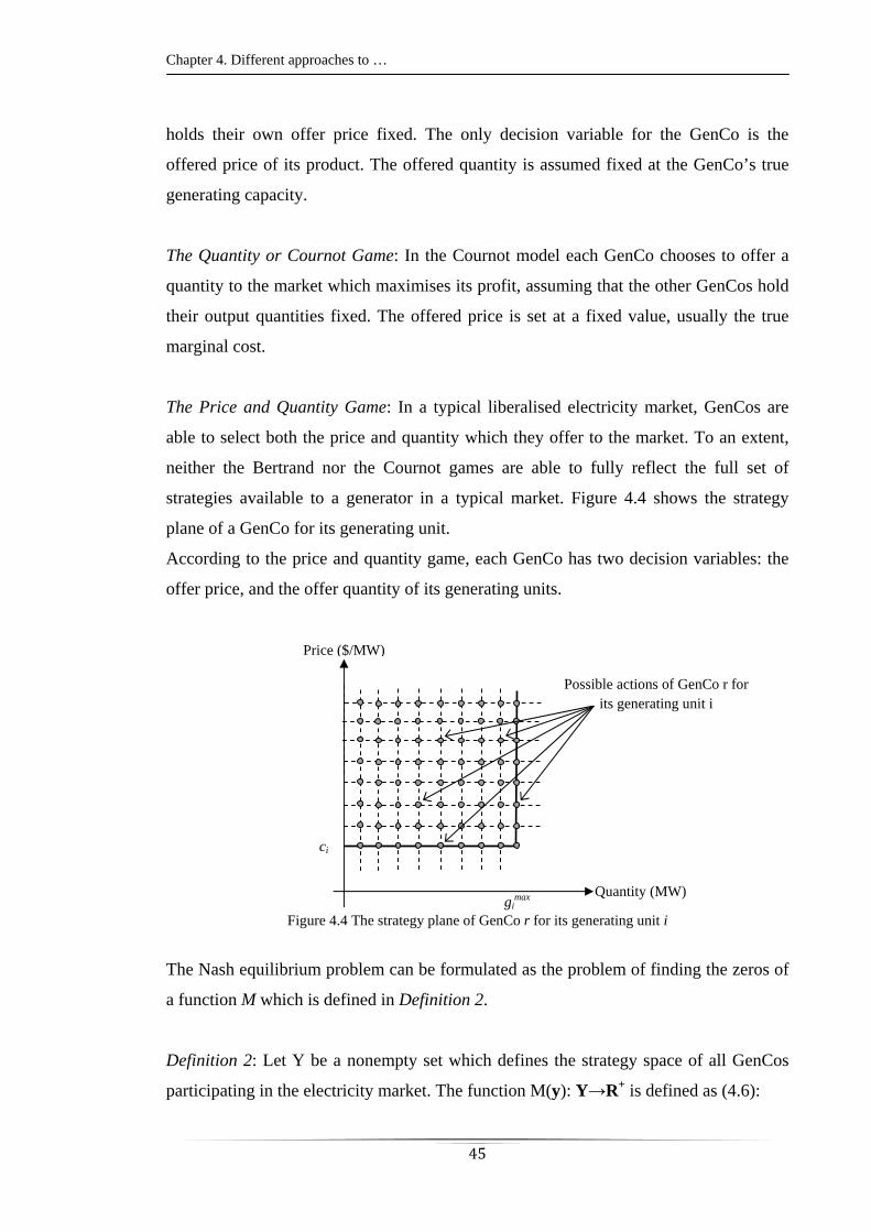
The Price and Quantity Game: In a typical liberalised electricity market, GenCos are
able to select both the price and quantity which they offer to the market. To an extent,
neither the Bertrand nor the Cournot games are able to fully reflect the full set of
strategies available to a generator in a typical market. Figure 4.4 shows the strategy
plane of a GenCo for its generating unit.
According to the price and quantity game, each GenCo has two decision variables: the
offer price, and the offer quantity of its generating units.
Figure 4.4 The strategy plane of GenCo r for its generating unit i
The Nash equilibrium problem can be formulated as the problem of finding the zeros of
a function M which is defined in Definition 2.
Definition 2: Let Y be a nonempty set which defines the strategy space of all GenCos
participating in the electricity market. The function M(y): Y→R+ is defined as (4.6):
Possible actions of GenCo r for its generating unit i
Quantity (MW)
Price ($/MW)
ci
gimax
Chapter 4. Different approaches to …
46
G
rr
N
rrrrrrrYy yyfyyfMaxyM
1
,, (4.6)
The following theorem can be derived consequently;
Theorem 1: The function M(y) : Y→R+ is real and nonnegative on Y. Also, the Nash
equilibria are the zeros of M.
Proof: Let yi be a strategy belonging to strategy space Yi and fi be the objective function
of player i in game G. Also, let y-i be the strategies of all other players of the game G
except player i. Define Mi(yi, y-i) = max fi(zi,y-i) - fi(yi,y-i) where the maximum is taken
over zi be a strategy belonging to strategy space Yi. Then Mi(yi, y-i) must be non-
negative by definition and is zero if and only if yi is a best response to the strategies y-i.
If we define M(y) = ∑ Mi then M(y)=0 if and only if y is a Nash equilibrium of the
game G.
It follows from Definition 2 and Theorem 1 that the set of Nash equilibria of this game
can be expressed as follows:
G
rr
N
rrrrrrrYyYyYy yyxfyyxfMaxMinyxMMinxY
1
* ,,,,),()( (4.7)
Mathematical structure in (4.7) is used for finding the Nash equilibria between the
generating companies participating in the market. In (4.7), fr is the GenCo r objective
function and y is its decision variables. We can conclude that the solutions to the
constrained optimisation problem in (4.8) are all Nash equilibria of the price and
quantity game among the GenCos. The mathematical structure in (4.8) is the expanded
version of (4.7). It is written based on the GenCos’ variables and the explicit
formulation of the economic dispatch problem.
Chapter 4. Different approaches to …
47
3max
2max
1max0
0
max,,,
maxmax
maxmin
1 1ˆ,ˆ
0
ˆ0
,
,0
..
ˆ
ˆ0
ˆ
..
max
uDkdd
uGkgg
uLjifnnf
Ljinnf
vdgB
ts
ddVoLLgcMin
gg
PcP
ts
gcvyfMaxMin
kk
kk
ijijijij
jiijijijij
Dkkkk
Gkkkfdg
ii
i
N
r
n
iiiirXxgc
ijkkk
GrG
ii
(4.8)
Step3: Formulation of the social planner’s problem
For any given transmission expansion plan and demand scenario, there are three
possible outcomes of the strategic game between the GenCos:
The game among GenCos has no equilibrium in pure strategies: In this case, the
analytical methods are not able to model the strategic behaviours of GenCos. This
research work assumes this case does not arise in practice.
The game among GenCos has only one equilibrium: The unique equilibrium of the
game can be found and used to model the strategic behaviours of GenCos.
The game among GenCos has multiple equilibria: This case poses a problem. How
should these multiple equilibria be handled?
Reference [110] uses an average method to deal with many Nash equilibria of the
quantity game among GenCos. This methodology calculates the market outcomes
(dispatch, price, flows, etc.) under each Nash equilibrium and then simply takes the
average over these values across all the different Nash equilibria. In effect, this
approach could be rationalised as a probability weighting over Nash equilibria where
each Nash equilibrium is assigned an equal probability of occurring. The problem with
this method is that a transmission augmentation is typically most valuable under

Chapter 4. Different approaches to …
48
extreme market conditions (high flows, high price differences). The process of
averaging by definition eliminates such extremes. In fact, even if flows are at their
limits in some Nash equilibria (in which case there would be value in an augmentation),
if flows are reversed in other Nash equilibria, the overall average flow may be close to
zero – suggesting that an augmentation has no value at all. For the purposes of
assessment of transmission augmentation, the averaging approach yields misleading
information.
In this research work the problem of multiple equilibria is handled using the concept of
the Stackelberg-Worst Nash Equilibrium introduced in Definition 1.
The TNSP finds the reaction of GenCos to its transmission expansion policy by
calculating the set of Nash equilibria of the price, and quantity game. The TNSP then
selects the Nash equilibrium which has the highest (worst) value in terms of its own
objective function. It then selects the transmission expansion policy which results in the
lowest (best) Worst-Nash Equilibrium.
Section 4.3 uses, as the objective function of the transmission planner, the monopoly
rent, MR, or an alternative metric termed L-Shape Area metric, AL. Both the monopoly
rent and the L-Shape Area metric are measures of market power.
The mathematical formulation of the worst Nash equilibrium in terms of the monopoly
rent and the L-Shape Area metric are set out in (4.9) and (4.10), respectively.
MRMingc maxˆ,ˆ
(4.9)
LgcAMin maxˆ,ˆ
(4.10)
4.2.1. Measuring market power using the concept of the quantity withheld Competitive markets were introduced into the electricity industry in order to reduce
prices, improve the quality of services, and on a long-term basis make the industry more
efficient, [111]. Ensuring effective competition between generators on one side of
market and between retailers on the other side is the necessary condition in achieving
the aforementioned targets.
The conditions required for perfect competition are, [112]:
(1) a large number of generators producing a homogeneous product;
(2) each generator attempts to maximise its payoff;
(3) each generator is a price taker;
Chapter 4. Different approaches to …
49
(4) generators have exact knowledge of all parameters of significance to their decisions;
(5) transmission is costless.
The first condition aims to prevent the formation of market concentration (as measured
by the Herfindahl-Hirshman Index) and pivotal generators (as measured by the Residual
Supply Index), [113]. It can be mathematically shown that a profit-maximising, price-
taking generator will offer its output to the dispatch process at its marginal cost, [115] .
Condition four says that the generators must have perfect information. Finally, the last
condition addresses bottlenecks in the high voltage transmission systems. Bottlenecks
are one of the major causes of market separation. Arguably, none of these conditions
ever exists in a real electricity market. Accordingly, the real electricity market deviates
from a theoretically ideal competitive electricity market.
GenCos can exercise market power in two ways: financial withholding and physical
withholding. Financial withholding means bidding excessively above the marginal cost
of production and driving up the price. Physical withholding arises when a GenCo
withholds some of its available capacity from the market thus reducing effective supply
and driving up the price it receives for the rest of its portfolio, [113].
Subsection 4.2.2 examines how market power might be measured through a metric
termed the L-Shape Area metric. The L-Shape Area metric is designed to capture both
forms of exercise of market power: financial withholding and physical withholding.
4.2.2 Design of the L-Shape Area Metric for measuring market power – application of the quantity withheld concept The L-Shape area metric is based on the notion of measuring the deviation of the
electricity market equilibrium from the competitive equilibrium.
Definition of L-Shape Area Metric (AL): Let vc and v be the non-empty vectors in Rn
representing nodal prices ($/MW) and let Gmax≠0 and G≠0 be the aggregated offered
capacity of GenCos (MW) in the following two scenarios;
(1) Competitive electricity market with relaxed transmission constraints and;
(2) Actual electricity market, respectively.
If Δv is the Euclidean norm of the vector vc - v as in (4.11),
2cvvv (4.11)
Then, AL 0 ($) is;
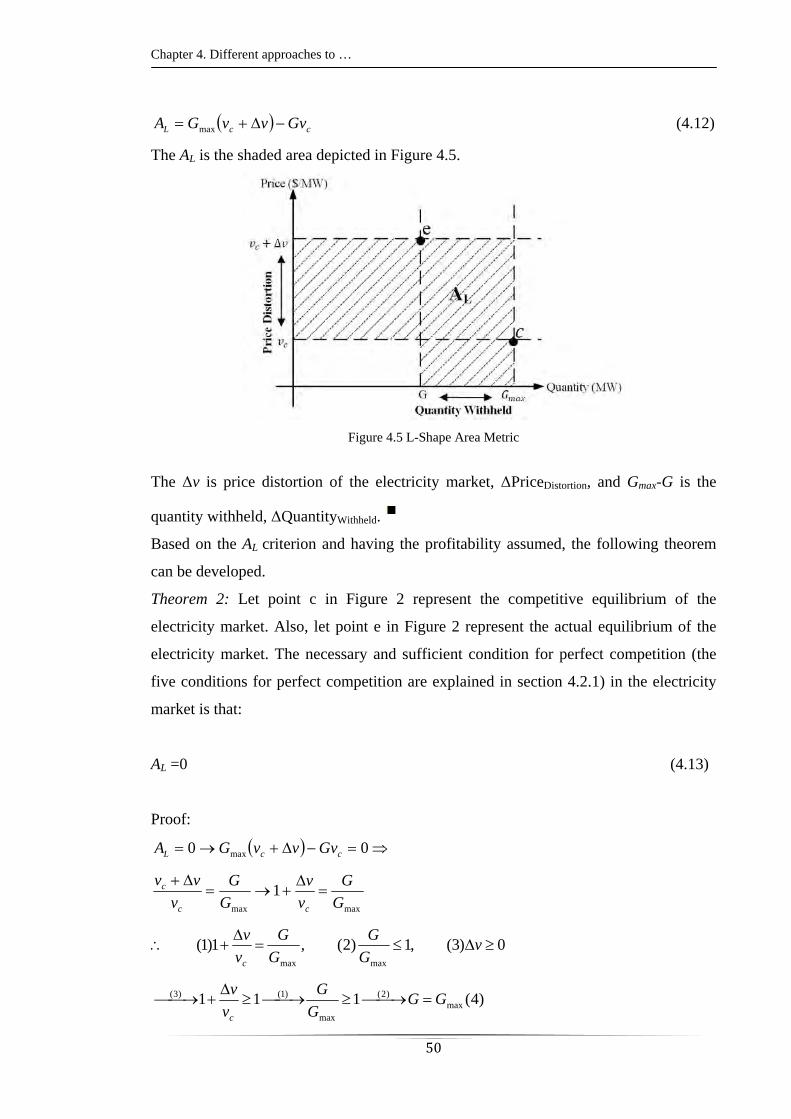
Chapter 4. Different approaches to …
50
ccL GvvvGA max (4.12)
The AL is the shaded area depicted in Figure 4.5.
Figure 4.5 L-Shape Area Metric
The Δv is price distortion of the electricity market, ΔPriceDistortion, and Gmax-G is the
quantity withheld, ΔQuantityWithheld.
Based on the AL criterion and having the profitability assumed, the following theorem
can be developed.
Theorem 2: Let point c in Figure 2 represent the competitive equilibrium of the
electricity market. Also, let point e in Figure 2 represent the actual equilibrium of the
electricity market. The necessary and sufficient condition for perfect competition (the
five conditions for perfect competition are explained in section 4.2.1) in the electricity
market is that:
AL =0 (4.13)
Proof:
00 max ccL GvvvGA
maxmax
1G
G
v
v
G
G
v
vv
cc
c
0)3(,1)2(,1)1(maxmax
vG
G
G
G
v
v
c
)4(111 max)2(
max
)1()3( GGG
G
v
v
c

Chapter 4. Different approaches to …
51
0002
)4()1( Lcand Avvv
In section 4.3, we approximate the competitive equilibrium of the electricity market by
finding the competitive equilibrium with relaxed transmission constraints. This reduces
the complexity of the associated constrained optimisation problem. Although this
approach is in line with [114], [115], and [116], this is a strong assumption. It may be
possible to remove this assumption with further research. One possible approach to
proceed is to find the AL metric for each node of the system.
The proposed constrained optimisation problem based on the metrics of quantity
withheld, AL, and the M function, is presented in (4.14).
In (4.14), cij is the transmission investment cost between nodes i and j, nij is an integer
number which represents the number of new circuits in the corridor i-j with a maximum
number of nijmax, gi
c is the competitive dispatch of the GenCo i, and dic is the
competitive dispatch of retailer i.
3max
2max
1max0
0
max,,,
maxmax
maxmin
1 1ˆ,ˆ
max
ˆ,ˆ),(
0
ˆ0
,
,0
..
ˆ
ˆ0
ˆ
..
,,0
..
][
max
max
uDkdd
uGkgg
uLjifnnf
Ljinnf
vdgB
ts
ddVoLLgcMin
gg
PcP
ts
gcvyfMaxMin
NnLjinn
ts
AMaxncMin
kk
kk
ijijijij
jiijijijij
Dkkkk
Gkkkfdg
ii
i
N
r
n
iiiirYygc
ijijij
LgcLji
ijijn
ijkkk
GrG
ii
kkij
(4.14)
Chapter 4. Different approaches to …
52
4.3. The competitive social cost and the monopoly rent Consumers are likely to be harmed by the strategic behaviours of GenCos. It is likely
that at least some consumers will face higher prices if some GenCos bid strategically.
Similarly, some GenCos will have higher profits under strategic bidding than they
would if all GenCos bid their marginal cost curve.
Monopoly rent is a consequence of exercising market power by GenCos. It is defined as
the excess profit that GenCos capture under strategic bidding behaviour compared to the
profit they would earn in a competitive equilibrium.
For the purposes of this research, the Monopoly Rent is defined as in (4.15),
GN
i
ciiMR
1
(4.15)
In (4.15), πi is the profit of the ith GenCo in the electricity market and πic is the profit of
the same GenCo in the competitive electricity market.
Mathematical structure of the TNSP augmentation mechanism
The proposed constrained optimisation problem for the assessment of transmission
system augmentations based on the Competitive Social Cost, the Monopoly Rent
metric, the M function is presented in (4.16).
In (4.16), cij is the transmission investment cost between nodes i and j, nij is an integer
number which represents the number of new circuits in the corridor i-j with a maximum
number of nijmax, gi
c is the competitive dispatch of the GenCo i, and dic is the
competitive dispatch of retailer i.

Chapter 4. Different approaches to …
53
3max
2max
1max0
0
max,,,
maxmax
maxmin
1 1ˆ,ˆ
max
ˆ,ˆ
max
),(
0
ˆ0
,
,0
..
ˆ
ˆ0
ˆ
..
,,0
..
][
max
max
uDkdd
uGkgg
uLjifnnf
Ljinnf
vdgB
ts
ddVoLLgcMin
gg
PcP
ts
gcvyfMaxMin
NnLjinn
ts
MRMaxddVoLLgcncMin
kk
kk
ijijijij
jiijijijij
Dkkkk
Gkkkfdg
ii
i
N
r
n
iiiirYygc
ijijij
gcGi Di
ciii
cii
Ljiijijn
ijkkk
GrG
ii
kkij
(4.16)
The minimisation problem, Mingc,d
c,θ
c,fij
c, is the security-constraint economic dispatch
under the competitive equilibrium of the electricity market. The dispatch results of the
competitive equilibrium of the electricity market, denoted by superscript “c” in (4.16),
are used to calculate the GenCos’ profit in the competitive equilibrium of the electricity
market. Also, the effect of transmission capacity on the efficiency of the electricity
market is found through the Mingc,d
c,θ
c,fij
c minimisation problem. The objective of this
minimisation problem is the total cost to the society at the competitive equilibrium of
the electricity market and is termed competitive social cost. Accordingly, the TNSP
objective function in (4.16), Γ, has three components, the transmission investment cost,
the competitive social cost, and the monopoly rent. The competitive social cost is used
to measure the impact of transmission capacity on the efficiency of the dispatch and the
monopoly rent as a metric of the market power exercised by GenCos.
Comparing the optimisation problem in (4.14) with (4.16) shows that introducing the AL
metric has reduced the mathematical structure from a three-level structure to a two-level
structure. This is because in calculating the MR index, we need to run the security-
constrained economic dispatch problem for two scenarios of the competitive bidding
Chapter 4. Different approaches to …
54
and strategic bidding. This adds another level to the optimisation problem, i.e. one more
level for modelling the competitive bidding in the structure.
Both (4.15) and (4.16) find the optimal transmission planning schedule for the worst
case senario in the horizon year of planning. The coefficient σ is the number of hours of
the worst case scenario in the horizon year of planning.
Both (4.15) and (4.16) only take into account a single scenario of the electricity market.
The relevant scenario of the electricity market for the sake of this research study can be
found using the “importance sampling technique” reported in [117]. The use of a single
scenario here helps to make the contribution of this work clear and avoids clouding the
issue with the uncertainties involved in the decision making process. However, the
extension of the problem to take into account demand and supply uncertainties can be
addressed in future research.
4.4. The economic concept of social cost – Part 1 This section uses the concept of the socially worst Nash equilibrium for the purposes of
transmission augmentation decisions. The worst Nash equilibrium is the one which has
the highest social cost to the society. The social cost is defined as the total cost of
generation and total value of lost load. The mathematical formulation of the worst Nash
equilibrium is set out in (4.17).
ii
Diii
Giigc
ddVoLLgcMaxii
max
ˆ,ˆ max (4.17)
In (4.17), the objective function is the total cost to the society which must be computed
for each of Nash equilibria of the GenCos’ price-quantity game.
Suppose L is the set of all upgrade and expansion projects available for the TNSP, cij is
the cost of transmission project between buses i and j and nij is the number of circuits in
the transmission corridor i-j. nijmax is the maximum value for the integer variable nij. The
vector n is the TNSP’s design parameter.
The constrained optimisation problem of the TNSP can be formulated as (4.18).
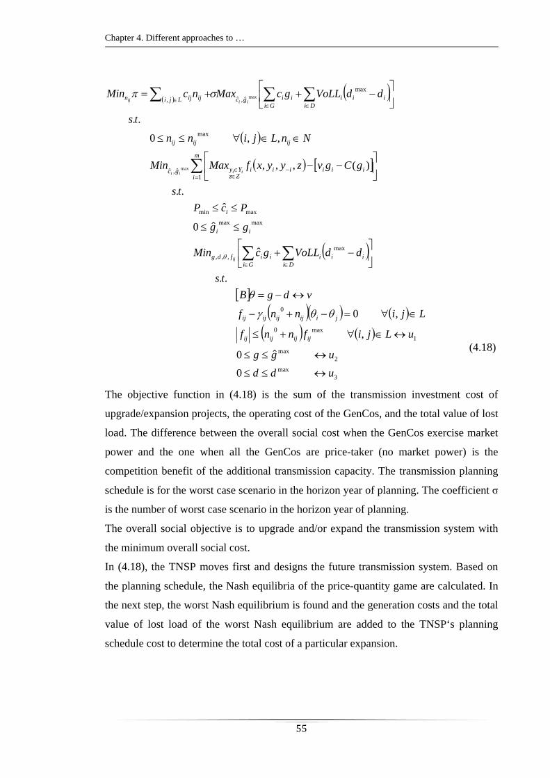
Chapter 4. Different approaches to …
55
3max
2max
1max0
0
max,,,
maxmax
maxmin
1ˆ,ˆ
max
max
ˆ,ˆ,
0
ˆ0
,
,0
..
ˆ
ˆ0
ˆ
..
)(,,,
,,0
..
max
max
udd
ugg
uLjifnnf
Ljinnf
vdgB
ts
ddVoLLgcMin
gg
PcP
ts
gCgvzyyxfMaxMin
NnLjinn
ts
ddVoLLgcMaxncMin
ijijijij
jiijijijij
iiDi
iiGi
ifdg
ii
i
m
iiiiiii
ZzYygc
ijijij
iiDi
iiGi
igcLji ijijn
ij
iiii
iiij
(4.18)
The objective function in (4.18) is the sum of the transmission investment cost of
upgrade/expansion projects, the operating cost of the GenCos, and the total value of lost
load. The difference between the overall social cost when the GenCos exercise market
power and the one when all the GenCos are price-taker (no market power) is the
competition benefit of the additional transmission capacity. The transmission planning
schedule is for the worst case scenario in the horizon year of planning. The coefficient σ
is the number of worst case scenario in the horizon year of planning.
The overall social objective is to upgrade and/or expand the transmission system with
the minimum overall social cost.
In (4.18), the TNSP moves first and designs the future transmission system. Based on
the planning schedule, the Nash equilibria of the price-quantity game are calculated. In
the next step, the worst Nash equilibrium is found and the generation costs and the total
value of lost load of the worst Nash equilibrium are added to the TNSP‘s planning
schedule cost to determine the total cost of a particular expansion.
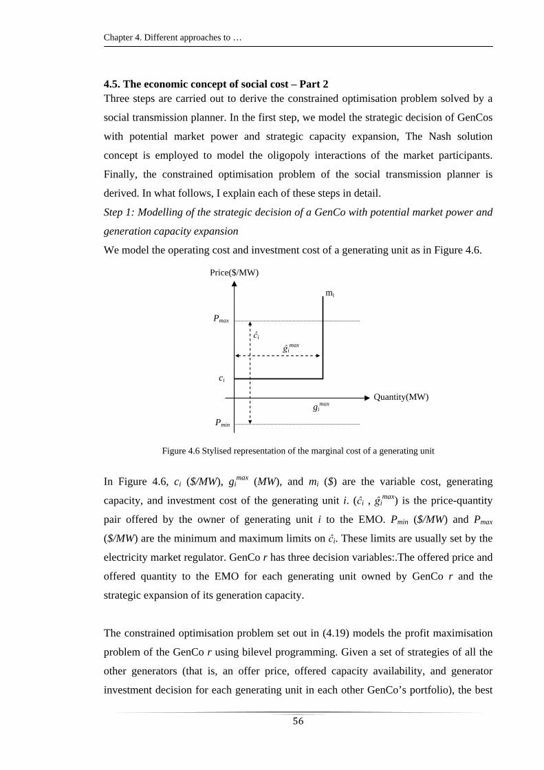
Chapter 4. Different approaches to …
56
4.5. The economic concept of social cost – Part 2 Three steps are carried out to derive the constrained optimisation problem solved by a
social transmission planner. In the first step, we model the strategic decision of GenCos
with potential market power and strategic capacity expansion, The Nash solution
concept is employed to model the oligopoly interactions of the market participants.
Finally, the constrained optimisation problem of the social transmission planner is
derived. In what follows, I explain each of these steps in detail.
Step 1: Modelling of the strategic decision of a GenCo with potential market power and
generation capacity expansion
We model the operating cost and investment cost of a generating unit as in Figure 4.6.
Figure 4.6 Stylised representation of the marginal cost of a generating unit
In Figure 4.6, ci ($/MW), gimax (MW), and mi ($) are the variable cost, generating
capacity, and investment cost of the generating unit i. (ĉi , ĝimax) is the price-quantity
pair offered by the owner of generating unit i to the EMO. Pmin ($/MW) and Pmax
($/MW) are the minimum and maximum limits on ĉi. These limits are usually set by the
electricity market regulator. GenCo r has three decision variables:.The offered price and
offered quantity to the EMO for each generating unit owned by GenCo r and the
strategic expansion of its generation capacity.
The constrained optimisation problem set out in (4.19) models the profit maximisation
problem of the GenCo r using bilevel programming. Given a set of strategies of all the
other generators (that is, an offer price, offered capacity availability, and generator
investment decision for each generating unit in each other GenCo’s portfolio), the best
Quantity(MW)
Price($/MW)
Pmin
Pmax
ci
ĉi
ĝimax
gimax
mi
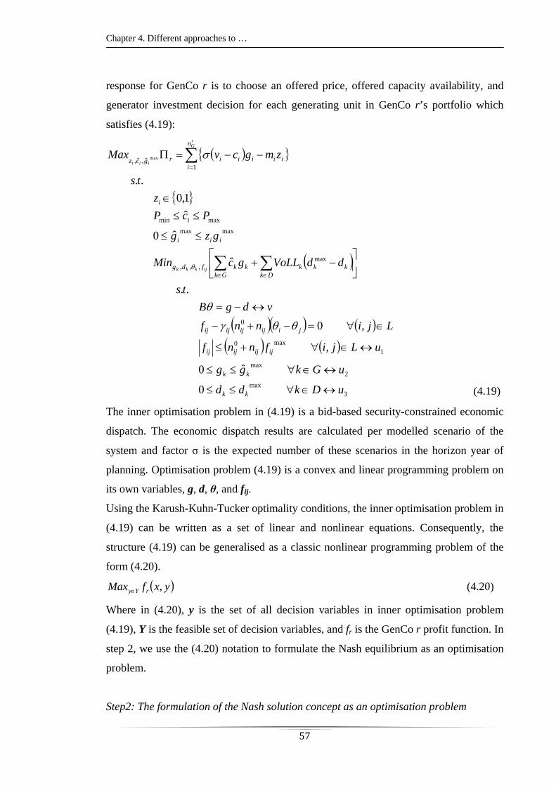
Chapter 4. Different approaches to …
57
response for GenCo r is to choose an offered price, offered capacity availability, and
generator investment decision for each generating unit in GenCo r’s portfolio which
satisfies (4.19):
3max
2max
1max0
0
max,,,
maxmax
maxmin
1ˆ,ˆ,
0
ˆ0
,
,0
..
ˆ
ˆ0
ˆ
1,0
..
max
uDkdd
uGkgg
uLjifnnf
Ljinnf
vdgB
ts
ddVoLLgcMin
gzg
PcP
z
ts
zmgcvMax
kk
kk
ijijijij
jiijijijij
Dkkkk
Gkkkfdg
iii
i
i
n
iiiiiirgcz
ijkkk
rG
iii
(4.19)
The inner optimisation problem in (4.19) is a bid-based security-constrained economic
dispatch. The economic dispatch results are calculated per modelled scenario of the
system and factor σ is the expected number of these scenarios in the horizon year of
planning. Optimisation problem (4.19) is a convex and linear programming problem on
its own variables, g, d, θ, and fij.
Using the Karush-Kuhn-Tucker optimality conditions, the inner optimisation problem in
(4.19) can be written as a set of linear and nonlinear equations. Consequently, the
structure (4.19) can be generalised as a classic nonlinear programming problem of the
form (4.20).
yxfMax rYy , (4.20)
Where in (4.20), y is the set of all decision variables in inner optimisation problem
(4.19), Y is the feasible set of decision variables, and fr is the GenCo r profit function. In
step 2, we use the (4.20) notation to formulate the Nash equilibrium as an optimisation
problem.
Step2: The formulation of the Nash solution concept as an optimisation problem
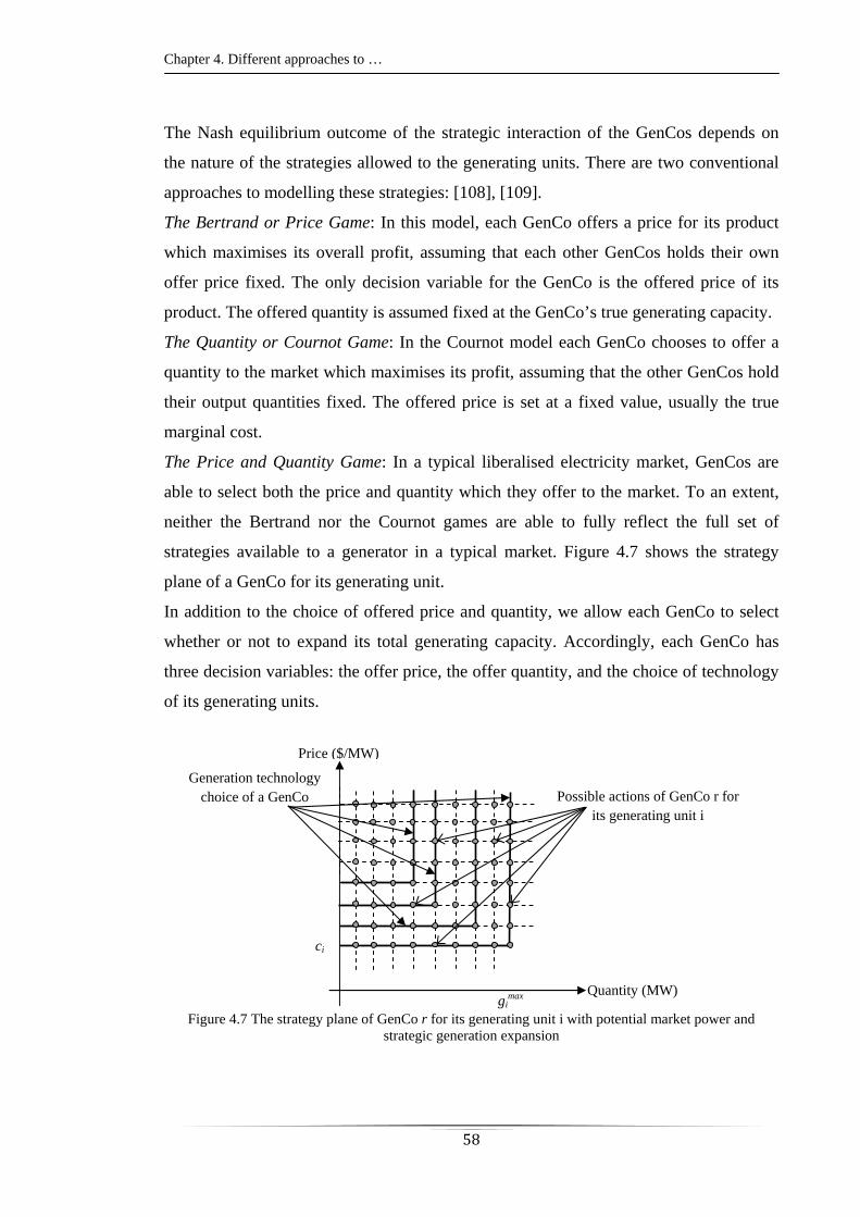
Chapter 4. Different approaches to …
58
The Nash equilibrium outcome of the strategic interaction of the GenCos depends on
the nature of the strategies allowed to the generating units. There are two conventional
approaches to modelling these strategies: [108], [109].
The Bertrand or Price Game: In this model, each GenCo offers a price for its product
which maximises its overall profit, assuming that each other GenCos holds their own
offer price fixed. The only decision variable for the GenCo is the offered price of its
product. The offered quantity is assumed fixed at the GenCo’s true generating capacity.
The Quantity or Cournot Game: In the Cournot model each GenCo chooses to offer a
quantity to the market which maximises its profit, assuming that the other GenCos hold
their output quantities fixed. The offered price is set at a fixed value, usually the true
marginal cost.
The Price and Quantity Game: In a typical liberalised electricity market, GenCos are
able to select both the price and quantity which they offer to the market. To an extent,
neither the Bertrand nor the Cournot games are able to fully reflect the full set of
strategies available to a generator in a typical market. Figure 4.7 shows the strategy
plane of a GenCo for its generating unit.
In addition to the choice of offered price and quantity, we allow each GenCo to select
whether or not to expand its total generating capacity. Accordingly, each GenCo has
three decision variables: the offer price, the offer quantity, and the choice of technology
of its generating units.
Figure 4.7 The strategy plane of GenCo r for its generating unit i with potential market power and strategic generation expansion
Possible actions of GenCo r for its generating unit i
Quantity (MW)
ci
gimax
Generation technology choice of a GenCo
Price ($/MW)

Chapter 4. Different approaches to …
59
It follows from Definition 2 and Theorem 1, that the set of Nash equilibria of this game
can be expressed as follows:
G
rr
N
rrrrrrrYyYyYy yyxfyyxfMaxMinyxMMinxY
1
* ,,,,),()( (4.21)
We can conclude that the constrained optimisation problem set out in (4.22) can
calculate all Nash equilibria of the price, quantity, and generation investment game
among the GenCos.
3max
2max
1max0
0
max,,,
maxmax
maxmin
1 1ˆ,ˆ,
0
ˆ0
,
,0
..
ˆ
ˆ0
ˆ
1,0
..
max
uDkdd
uGkgg
uLjifnnf
Ljinnf
vdgB
ts
ddVoLLgcMin
gzg
PcP
z
ts
zmgcvyfMaxMin
kk
kk
ijijijij
jiijijijij
Dkkkk
Gkkkfdg
iii
i
i
N
r
n
iiiiiirXxgcz
ijkkk
GrG
iii
(4.22)
Step3: Formulation of the social planner problem
The TNSP finds the reaction of GenCos to its transmission expansion policy by
calculating the set of Nash equilibria of the price, quantity and generation investment
game. The TNSP then selects the Nash equilibrium which has the highest social cost.
The social cost is defined as the sum of the operating cost and investment cost. The
operating cost is the sum of generating cost and the total value of lost load. The
investment cost is the sum of the transmission investment cost and the generation
investment cost. The transmission policy which has the minimum of the maximum
social cost is selected as the optimal decision of the TNSP.
This process is modelled in (4.23) as an integrated mathematical structure.
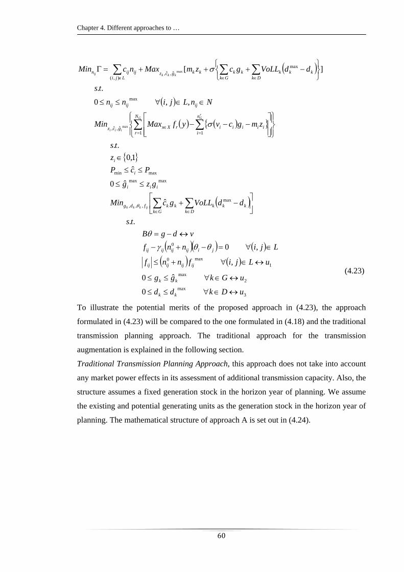
Chapter 4. Different approaches to …
60
3max
2max
1max0
0
max,,,
maxmax
maxmin
1 1ˆ,ˆ,
max
max
ˆ,ˆ,),(
0
ˆ0
,
,0
..
ˆ
ˆ0
ˆ
1,0
..
,,0
..
][
max
max
uDkdd
uGkgg
uLjifnnf
Ljinnf
vdgB
ts
ddVoLLgcMin
gzg
PcP
z
ts
zmgcvyfMaxMin
NnLjinn
ts
ddVoLLgczmMaxncMin
kk
kk
ijijijij
jiijijijij
Dkkkk
Gkkkfdg
iii
i
i
N
r
n
iiiiiirXxgcz
ijijij
Dkkkk
Gkkkkkgcz
Ljiijijn
ijkkk
GrG
iii
kkkij
(4.23)
To illustrate the potential merits of the proposed approach in (4.23), the approach
formulated in (4.23) will be compared to the one formulated in (4.18) and the traditional
transmission planning approach. The traditional approach for the transmission
augmentation is explained in the following section.
Traditional Transmission Planning Approach, this approach does not take into account
any market power effects in its assessment of additional transmission capacity. Also, the
structure assumes a fixed generation stock in the horizon year of planning. We assume
the existing and potential generating units as the generation stock in the horizon year of
planning. The mathematical structure of approach A is set out in (4.24).
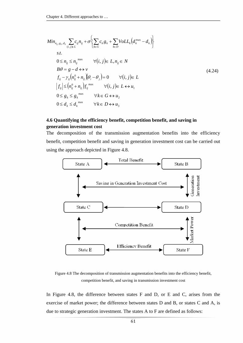
Chapter 4. Different approaches to …
61
3max
2max
1max0
0
max
max
),(,,
0
0
,
,0
,,0
..
uDkdd
uGkgg
uLjifnnf
Ljinnf
vdgB
NnLjinn
ts
ddVoLLgcncMin
kk
kk
ijijijij
jiijijijij
ijijij
Dkkkk
Gkkk
Ljiijijdgn kkij
(4.24)
4.6 Quantifying the efficiency benefit, competition benefit, and saving in generation investment cost The decomposition of the transmission augmentation benefits into the efficiency
benefit, competition benefit and saving in generation investment cost can be carried out
using the approach depicted in Figure 4.8.
Figure 4.8 The decomposition of transmission augmentation benefits into the efficiency benefit,
competition benefit, and saving in transmission investment cost
In Figure 4.8, the difference between states F and D, or E and C, arises from the
exercise of market power; the difference between states D and B, or states C and A, is
due to strategic generation investment. The states A to F are defined as follows:
Chapter 4. Different approaches to …
62
State A: Social cost of the electricity market, given strategic generators with strategic
generation investment and the status quo transmission system
State B: Social cost of the electricity market, given strategic generators with strategic
generation investment and the augmented transmission system
State C: Social cost of the electricity market, given strategic generators and the status
quo transmission system
State D: Social cost of the electricity market, given strategic generators and the
augmented transmission system
State E: Social cost of the electricity market, given competitive generators and the status
quo transmission system
State F: Social cost of the electricity market, given competitive generators and the
augmented transmission system
Based on the states definitions in Figure 4.8, the efficiency benefit, the competition
benefit, and the saving in investment cost is defined as in (4.25), (4.26), and (4.27),
respectively.
Efficiency Benefit = ΓF – ΓE (4.25)
Competition Benefit = | ΓD – ΓF | – | ΓC – ΓE | (4.26)
Saving in Generation Investment Cost = | ΓB – ΓD | – | ΓA – ΓC | (4.27)
In (4.25), (4.26), and (4.27), Γ is the TNSP’s objective function. The total benefit of an
additional transmission capacity is sum of the efficiency benefit, competition benefit,
and the saving in generation investment cost. The total benefit is ΓB – ΓA as in Figure
4.8.
4.7 A comparative study of the four proposed approaches
In Table 4.1 three of the four proposed approaches in the previous sections of this
chapter are compared and the best one is highlighted.
Table 4.1 A comparative study of the first three approaches proposed by this research work
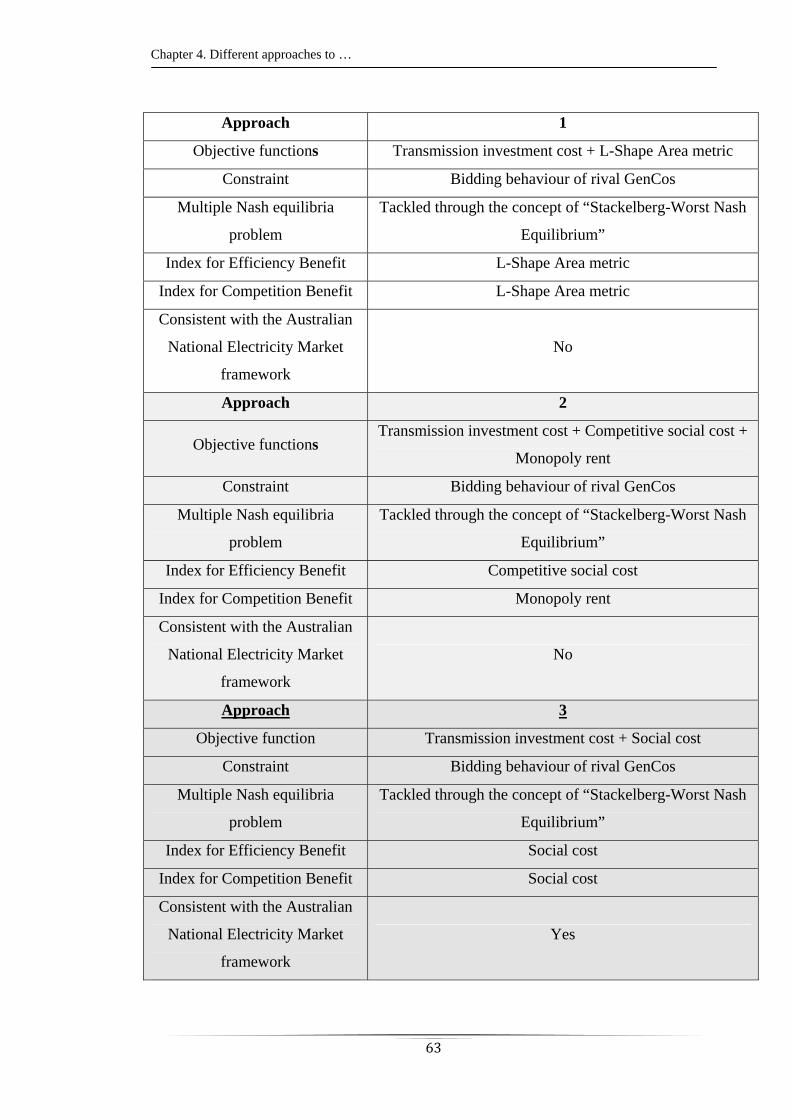
Chapter 4. Different approaches to …
63
Approach 1
Objective functions Transmission investment cost + L-Shape Area metric
Constraint Bidding behaviour of rival GenCos
Multiple Nash equilibria
problem
Tackled through the concept of “Stackelberg-Worst Nash
Equilibrium”
Index for Efficiency Benefit L-Shape Area metric
Index for Competition Benefit L-Shape Area metric
Consistent with the Australian
National Electricity Market
framework
No
Approach 2
Objective functions Transmission investment cost + Competitive social cost +
Monopoly rent
Constraint Bidding behaviour of rival GenCos
Multiple Nash equilibria
problem
Tackled through the concept of “Stackelberg-Worst Nash
Equilibrium”
Index for Efficiency Benefit Competitive social cost
Index for Competition Benefit Monopoly rent
Consistent with the Australian
National Electricity Market
framework
No
Approach 3
Objective function Transmission investment cost + Social cost
Constraint Bidding behaviour of rival GenCos
Multiple Nash equilibria
problem
Tackled through the concept of “Stackelberg-Worst Nash
Equilibrium”
Index for Efficiency Benefit Social cost
Index for Competition Benefit Social cost
Consistent with the Australian
National Electricity Market
framework
Yes
Chapter 4. Different approaches to …
64
Among the above three approaches, approach 3 is the one which is suggested by this
research proposal. It
(1) is consistent with current framework of the Australian National Electricity Market;
(2) has a sound economic foundation;
(3) has a single function in the TNSP objective function (mathematically, it is a single-
objective optimisation problem);
(4) can employ the decomposition technique introduced by the Australian Energy
Regulator.
Approach 4 is the extension of the approach 3 for modelling the strategic generation
investment decisions.
4.8 Chapter summary
In this chapter, we proposed four different approaches to the assessment of transmission
augmentation in liberalised electricity markets. The first structure employs the concepts
of the financial withholding and physical withholding in a metric termed the L-Shape
area metric. The L-Shape area metric measures the extent of deviation of the real
electricity market from a competitive one. The second approach uses the concept of
competitive social cost as a measure of the efficiency and monopoly rent as a measure
of the competitiveness of the market. The economic concept of social welfare or social
cost is employed for deriving the third and fourth mathematical structures. The third
mathematical structure models the efficiency benefit and competition benefit of the
additional transmission capacity. The fourth approach takes into account the benefits of
additional transmission capacity for increasing of the electricity market efficiency,
reducing market power, and preventing inefficient expansion of the generation sector.
An approach is proposed to decompose the total benefit of additional transmission
capacity into the efficiency benefit, the competition benefit, and saving in generation
investment cost.
Between the first three approaches, approach 3 is considered to have the most merit. It
(1) is consistent with current framework of the Australian National Electricity Market,
(2) has a sound economic foundation, (3) has a single function for the TNSP objective,
mathematically it is a single objective optimisation problem, and (4) can employ the
decomposition technique introduced by the Australian Energy Regulator.
Chapter 4. Different approaches to …
65
Approach 4 is the extension of the approach 3 for modelling the strategic generation
investment decisions.
These constrained optimisation approaches are analysed and discussed further in chapter
5.

CHAPTER 5 – THE NUMERICAL SOLUTION
TECHNIQUE
Chapter 5. The numerical solution technique
67
5.1 Introduction
This chapter deals with design and implementation of an optimisation technique for
solving the constrained optimisation problems set out in chapter 4. The proposed
optimisation algorithm is based on the Genetic Algorithm concept and operators. The
optimisation algorithm proposed here is termed a “Hybrid Bilevel Genetic
Algorithm/Island Parallel Genetic Algorithm” or HB GA/IPGA. The upper level
optimisation algorithm deals with the TNSP’s decision variables while the IPGA finds
the set of Nash equilibria of the rival GenCos.
The different stages of the HB GA/IPGA can be parallelised to improve performance. In
doing so, two major High Performance Computing, HPC, architectures are employed:
“Shared-memory architecture”, and “Distributed-memory architecture”.
The shared-memory architecture is implemented through the OpenMP application
program interface. The distributed-memory architecture is implemented using the
Message Passing Interface, MPI, library.
The algorithm of the HB GA/IPGA is explained in section 5.2 below. Section 5.3 uses
shared-memory architecture to parallelise the HB GA/IPGA. Distributed-memory
architecture and its application in parallelising the HB GA/IPGA is detailed in section
5.4. Section 5.5 concludes this chapter.
5.2 The Hybrid Bilevel Genetic Algorithm/Island Parallel Genetic Algorithm
Generally, optimisation algorithms can be divided in two classes: deterministic and
stochastic algorithms, [118], [119], and [120]. State space search, branch and bound,
and algebraic geometry are examples of deterministic approaches. The Monte Carlo
algorithm, evolutionary computation, and swarm intelligence are classified as stochastic
algorithms. Because of the complexity of the developed structures in chapter 4, which
stems from the nested optimisation and the high dimensionality of the search space, the
use of deterministic is unlikely to be practical. Also, the optimisation problems derived
in chapter 4 feature non-convex constraints. Therefore, we can not simply write down
the necessary and sufficient conditions and solve them directly. To reduce the
complexity of these problems and to make them more suitable for stochastic
optimization approaches, the price-quantity pairs offered by GenCos are approximated
by discrete variables. Next, a stochastic optimisation algorithm termed a Hybrid Bi-
Chapter 5. The numerical solution technique
68
Level Genetic Algorithm/Island Parallel Genetic Algorithm, GA/IPGA, is designed to
find a near-optimum solution of the optimisation problems in chapter 4.
In the Hybrid Bi-Level GA/IPGA, the GA deals with the TNSP decision variables and
the IPGA deals with the decision variables of the electricity market. The flowchart of
the Hybrid Bi-Level GA/IPGA is illustrated in Figure 5.1.
As in Figure 5.1, the Hybrid Bi-Level GA/IPGA starts with the initialisation of the
parent population. Next, each of the transmission planning schedules is evaluated based
on the investment cost and the worst social cost of the electricity market outcome. The
latter cost is calculated using the IPGA procedure. Using the crossover, mutation, and
selection operators of the standard GA, the population evolves towards the better
TNSP’s designs. The Hybrid Bi-Level GA/IPGA stops if the algorithm cannot improve
the objective function of the TNSP. The inequality |πj - πj-1|≤є in Figure 5.1 represents
this termination criterion. Finally, the best-found planning schedule is displayed.
An Island Parallel Genetic Algorithm, IPGA, is embedded in the algorithm of Figure
5.1 for solving the multimodal optimization problem introduced by the M function. The
techniques developed for solving problems of this type fall into three broad categories,
[121].
Iterative methods, [122], [123]:
Iterative methods address the problem of locating multiple optima of a multimodal
function by repeatedly applying the same optimization algorithm. To prevent repeated
convergence to the same solution, iterative methods use various techniques to prohibit
the underlying optimisation method from exploring the already explored areas.
Parallel Islands, [124], [125]:
This method tries to produce multiple solutions to a multimodal optimisation problem
by forming parallel populations which evolve in parallel. The parallel islands method
uses some communication topology to allow good characteristics of individuals to be
spread across islands.
Fitness sharing, [126], [127]:
The idea of sharing comes from an analogy with nature. In natural ecosystems, there are
many different ways in which species may survive and form different roles. Each role is
an ecological niche. The analogy in function optimisation is that the location of each
optimum represents a niche, and by suitably sharing the fitness associated with each
niche, we can encourage the formation of stable sub-populations at each optimum.
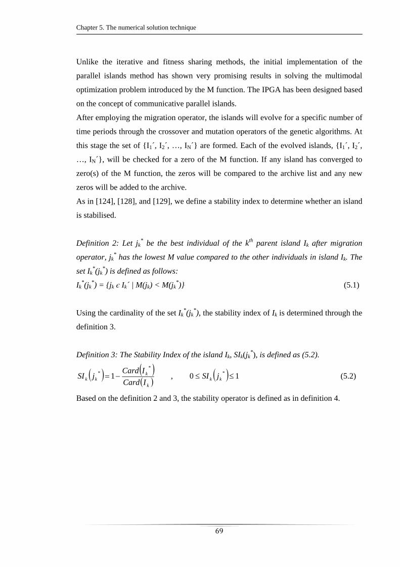
Chapter 5. The numerical solution technique
69
Unlike the iterative and fitness sharing methods, the initial implementation of the
parallel islands method has shown very promising results in solving the multimodal
optimization problem introduced by the M function. The IPGA has been designed based
on the concept of communicative parallel islands.
After employing the migration operator, the islands will evolve for a specific number of
time periods through the crossover and mutation operators of the genetic algorithms. At
this stage the set of I1´, I2´, …, IN´ are formed. Each of the evolved islands, I1´, I2´,
…, IN´, will be checked for a zero of the M function. If any island has converged to
zero(s) of the M function, the zeros will be compared to the archive list and any new
zeros will be added to the archive.
As in [124], [128], and [129], we define a stability index to determine whether an island
is stabilised.
Definition 2: Let jk* be the best individual of the kth parent island Ik after migration
operator, jk* has the lowest M value compared to the other individuals in island Ik. The
set Ik*(jk
*) is defined as follows:
Ik*(jk
*) = jk є Ik´ | M(jk) < M(jk*) (5.1)
Using the cardinality of the set Ik*(jk
*), the stability index of Ik is determined through the
definition 3.
Definition 3: The Stability Index of the island Ik, SIk(jk*), is defined as (5.2).
10,1 *
** kk
k
kkk jSI
ICard
ICardjSI (5.2)
Based on the definition 2 and 3, the stability operator is defined as in definition 4.
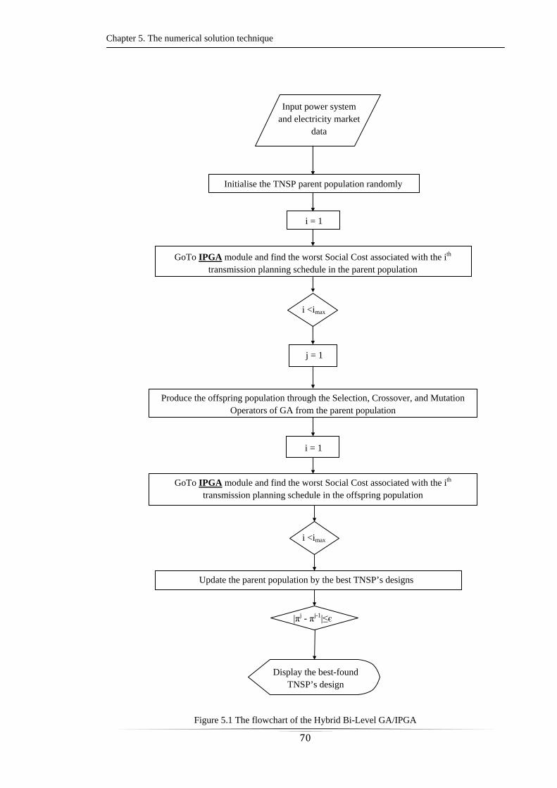
Chapter 5. The numerical solution technique
70
Figure 5.1 The flowchart of the Hybrid Bi-Level GA/IPGA
Input power system and electricity market
data
Initialise the TNSP parent population randomly
i = 1
GoTo IPGA module and find the worst Social Cost associated with the ith transmission planning schedule in the parent population
i <imax
i = 1
GoTo IPGA module and find the worst Social Cost associated with the ith transmission planning schedule in the offspring population
i <imax
Update the parent population by the best TNSP’s designs
Display the best-found TNSP’s design
|πj - πj-1|≤є
j = 1
Produce the offspring population through the Selection, Crossover, and Mutation Operators of GA from the parent population
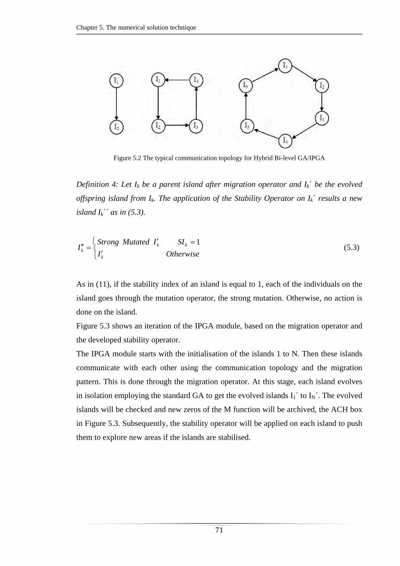
Chapter 5. The numerical solution technique
71
Figure 5.2 The typical communication topology for Hybrid Bi-level GA/IPGA
Definition 4: Let Ik be a parent island after migration operator and Ik´ be the evolved
offspring island from Ik. The application of the Stability Operator on Ik´ results a new
island Ik´´ as in (5.3).
OtherwiseI
SIIMutatedStrongI
k
kkk
1 (5.3)
As in (11), if the stability index of an island is equal to 1, each of the individuals on the
island goes through the mutation operator, the strong mutation. Otherwise, no action is
done on the island.
Figure 5.3 shows an iteration of the IPGA module, based on the migration operator and
the developed stability operator.
The IPGA module starts with the initialisation of the islands 1 to N. Then these islands
communicate with each other using the communication topology and the migration
pattern. This is done through the migration operator. At this stage, each island evolves
in isolation employing the standard GA to get the evolved islands I1´ to IN´. The evolved
islands will be checked and new zeros of the M function will be archived, the ACH box
in Figure 5.3. Subsequently, the stability operator will be applied on each island to push
them to explore new areas if the islands are stabilised.
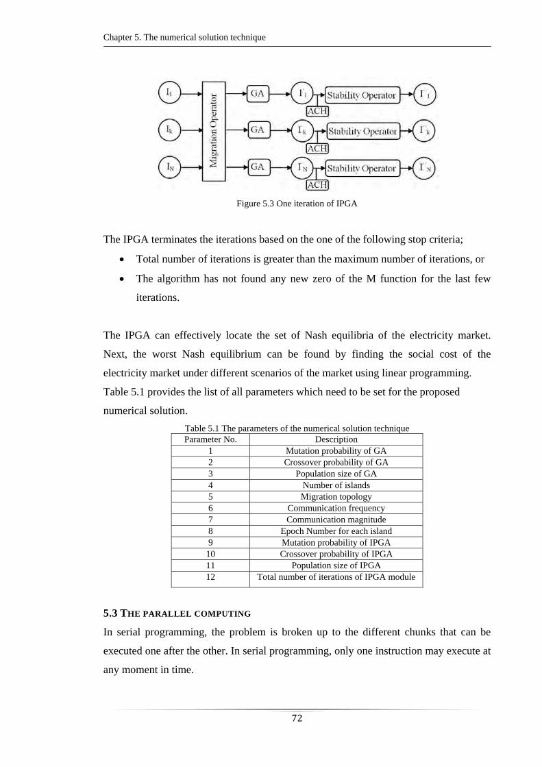
Chapter 5. The numerical solution technique
72
Figure 5.3 One iteration of IPGA
The IPGA terminates the iterations based on the one of the following stop criteria;
Total number of iterations is greater than the maximum number of iterations, or
The algorithm has not found any new zero of the M function for the last few
iterations.
The IPGA can effectively locate the set of Nash equilibria of the electricity market.
Next, the worst Nash equilibrium can be found by finding the social cost of the
electricity market under different scenarios of the market using linear programming.
Table 5.1 provides the list of all parameters which need to be set for the proposed
numerical solution.
Table 5.1 The parameters of the numerical solution technique Parameter No. Description
1 Mutation probability of GA 2 Crossover probability of GA 3 Population size of GA 4 Number of islands 5 Migration topology 6 Communication frequency 7 Communication magnitude 8 Epoch Number for each island 9 Mutation probability of IPGA
10 Crossover probability of IPGA 11 Population size of IPGA 12 Total number of iterations of IPGA module
5.3 THE PARALLEL COMPUTING
In serial programming, the problem is broken up to the different chunks that can be
executed one after the other. In serial programming, only one instruction may execute at
any moment in time.
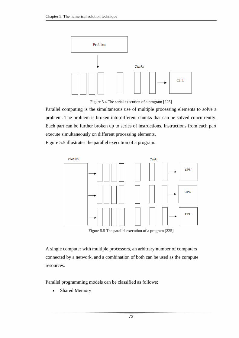
Chapter 5. The numerical solution technique
73
Figure 5.4 The serial execution of a program [225]
Parallel computing is the simultaneous use of multiple processing elements to solve a
problem. The problem is broken into different chunks that can be solved concurrently.
Each part can be further broken up to series of instructions. Instructions from each part
execute simultaneously on different processing elements.
Figure 5.5 illustrates the parallel execution of a program.
Figure 5.5 The parallel execution of a program [225]
A single computer with multiple processors, an arbitrary number of computers
connected by a network, and a combination of both can be used as the compute
resources.
Parallel programming models can be classified as follows;
Shared Memory

Chapter 5. The numerical solution technique
74
In the shared-memory programming model, a common address is shared by
different instructions of a program. Locks and semaphores are two methods of
controlling access to the shared memory.
In this model of parallel programming, there is no need to explicitly specify the
communication of data between parallel instructions. An advantage of this model
from the programmer’s point of view is that the notion of “data ownership” is
lacking. A disadvantage of this model of parallel programming is the difficulty in
understanding and managing data locality.
Threads
In this model, the program is first broken up to parallel regions. The master
thread executes the program until when it faces a parallel region. Then, the
master thread creates a team of threads called slave threads. Each thread runs a
part of parallel region in parallel with other threads. Threads communicate with
each other through global memory. After finishing the parallel region, the slave
threads join together and the master thread leaves the parallel region.
From a programming point of view, thread implementations commonly include:
A library of subroutines that are called from within parallel source code,
A set of compiler directives imbedded in either serial or parallel source
code
OpenMP is an implementation of the Threads model of parallel programming.
Message Passing
In the message passing model, processing elements use their own local memory
during computation. In this model, processing elements exchange data through
communication network. Data transfer usually requires cooperative operations to
be done by each processing element. For example, a send operation must have a
matching receive operation.
Figure 5.6 shows an example of the message passing model of parallel
programming.
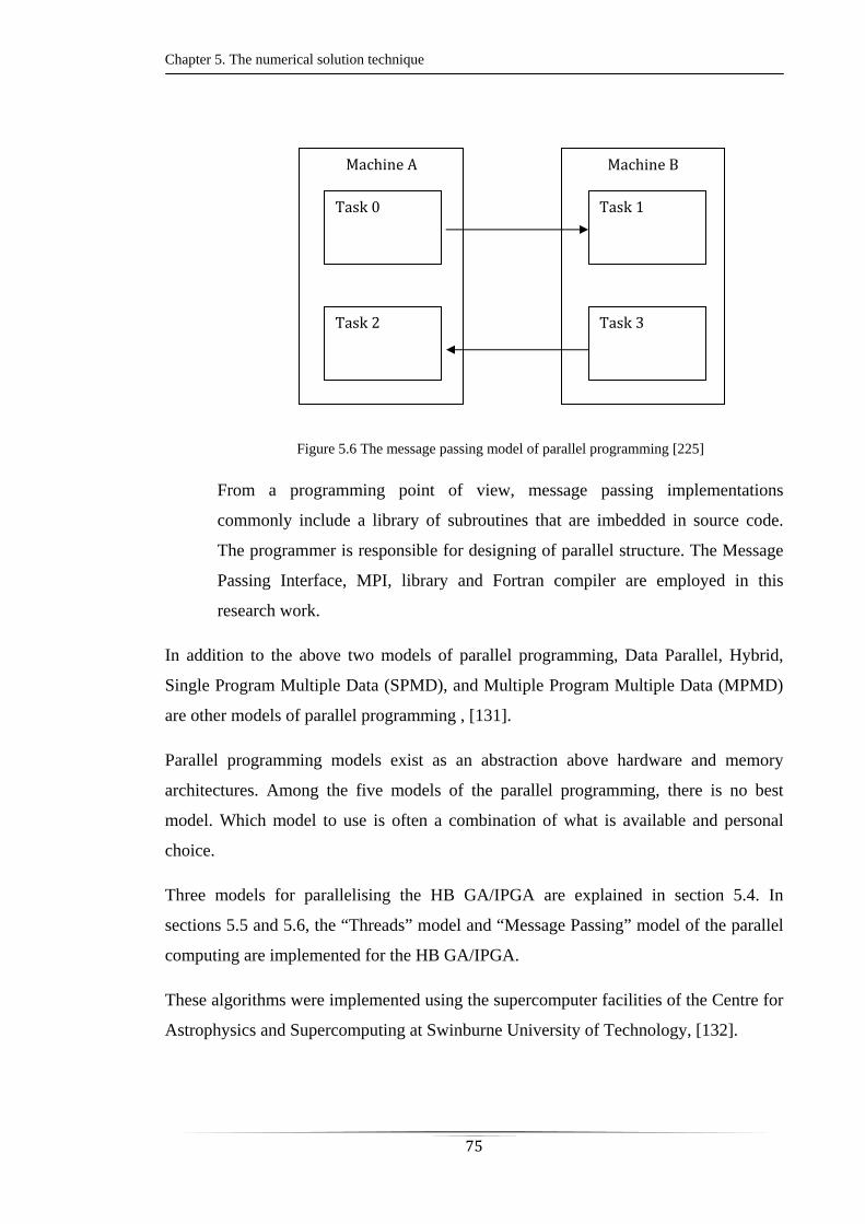
Chapter 5. The numerical solution technique
75
Figure 5.6 The message passing model of parallel programming [225]
From a programming point of view, message passing implementations
commonly include a library of subroutines that are imbedded in source code.
The programmer is responsible for designing of parallel structure. The Message
Passing Interface, MPI, library and Fortran compiler are employed in this
research work.
In addition to the above two models of parallel programming, Data Parallel, Hybrid,
Single Program Multiple Data (SPMD), and Multiple Program Multiple Data (MPMD)
are other models of parallel programming , [131].
Parallel programming models exist as an abstraction above hardware and memory
architectures. Among the five models of the parallel programming, there is no best
model. Which model to use is often a combination of what is available and personal
choice.
Three models for parallelising the HB GA/IPGA are explained in section 5.4. In
sections 5.5 and 5.6, the “Threads” model and “Message Passing” model of the parallel
computing are implemented for the HB GA/IPGA.
These algorithms were implemented using the supercomputer facilities of the Centre for
Astrophysics and Supercomputing at Swinburne University of Technology, [132].
MachineA
MachineB
Task0
Task2
Task1
Task3
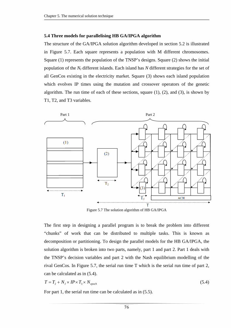
Chapter 5. The numerical solution technique
76
5.4 Three models for parallelising HB GA/IPGA algorithm
The structure of the GA/IPGA solution algorithm developed in section 5.2 is illustrated
in Figure 5.7. Each square represents a population with M different chromosomes.
Square (1) represents the population of the TNSP’s designs. Square (2) shows the initial
population of the NI different islands. Each island has N different strategies for the set of
all GenCos existing in the electricity market. Square (3) shows each island population
which evolves IP times using the mutation and crossover operators of the genetic
algorithm. The run time of each of these sections, square (1), (2), and (3), is shown by
T1, T2, and T3 variables.
Figure 5.7 The solution algorithm of HB GA/IPGA
The first step in designing a parallel program is to break the problem into different
“chunks” of work that can be distributed to multiple tasks. This is known as
decomposition or partitioning. To design the parallel models for the HB GA/IPGA, the
solution algorithm is broken into two parts, namely, part 1 and part 2. Part 1 deals with
the TNSP’s decision variables and part 2 with the Nash equilibrium modelling of the
rival GenCos. In Figure 5.7, the serial run time T which is the serial run time of part 2,
can be calculated as in (5.4).
epochI NTIPNTT 32 (5.4)
For part 1, the serial run time can be calculated as in (5.5).
Part 1 Part 2
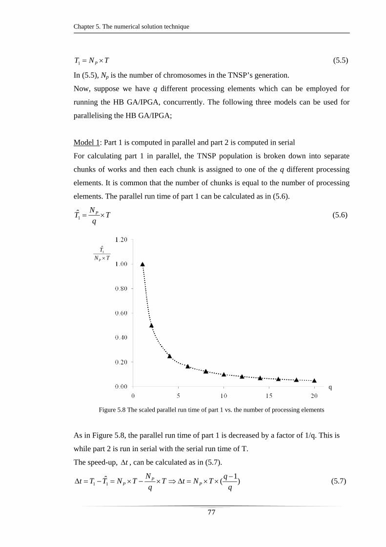
Chapter 5. The numerical solution technique
77
TNT P 1 (5.5)
In (5.5), Np is the number of chromosomes in the TNSP’s generation.
Now, suppose we have q different processing elements which can be employed for
running the HB GA/IPGA, concurrently. The following three models can be used for
parallelising the HB GA/IPGA;
Model 1: Part 1 is computed in parallel and part 2 is computed in serial
For calculating part 1 in parallel, the TNSP population is broken down into separate
chunks of works and then each chunk is assigned to one of the q different processing
elements. It is common that the number of chunks is equal to the number of processing
elements. The parallel run time of part 1 can be calculated as in (5.6).
Tq
NT P 1 (5.6)
Figure 5.8 The scaled parallel run time of part 1 vs. the number of processing elements
As in Figure 5.8, the parallel run time of part 1 is decreased by a factor of 1/q. This is
while part 2 is run in serial with the serial run time of T.
The speed-up, t , can be calculated as in (5.7).
)1
(11 q
qTNtT
q
NTNTTt P
PP
(5.7)
q
TN
T
P 1
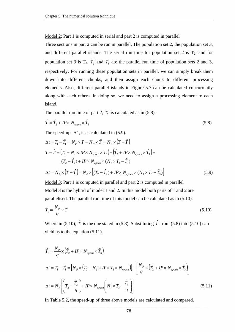
Chapter 5. The numerical solution technique
78
Model 2: Part 1 is computed in serial and part 2 is computed in parallel
Three sections in part 2 can be run in parallel. The population set 2, the population set 3,
and different parallel islands. The serial run time for population set 2 is T2, and for
population set 3 is T3. 2T and 3T are the parallel run time of population sets 2 and 3,
respectively. For running these population sets in parallel, we can simply break them
down into different chunks, and then assign each chunk to different processing
elements. Also, different parallel islands in Figure 5.7 can be calculated concurrently
along with each others. In doing so, we need to assign a processing element to each
island.
The parallel run time of part 2, 2T is calculated as in (5.8).
32ˆˆˆ TNIPTT epoch (5.8)
The speed-up, t , is as calculated in (5.9).
TTNTNTNTTt PPPˆˆ
11
)ˆ()ˆ(
ˆˆˆ
3322
3232
TTNNIPTT
TNIPTTNIPNTTT
Iepoch
epochepochI
)ˆ()ˆ(ˆ3322 TTNNIPTTNTTNt IepochPP (5.9)
Model 3: Part 1 is computed in parallel and part 2 is computed in parallel
Model 3 is the hybrid of model 1 and 2. In this model both parts of 1 and 2 are
parallelised. The parallel run time of this model can be calculated as in (5.10).
Tq
NT P ˆ
1 (5.10)
Where in (5.10), T is the one stated in (5.8). Substituting T from (5.8) into (5.10) can
yield us to the equation (5.11).
321ˆˆˆ TNIPT
q
NT epoch
P
323211
ˆˆˆ TNIPTq
NNTIPNTNTTt epoch
PepochIP
q
TTNNIP
q
TTNt IepochP
33
22
ˆˆ (5.11)
In Table 5.2, the speed-up of three above models are calculated and compared.
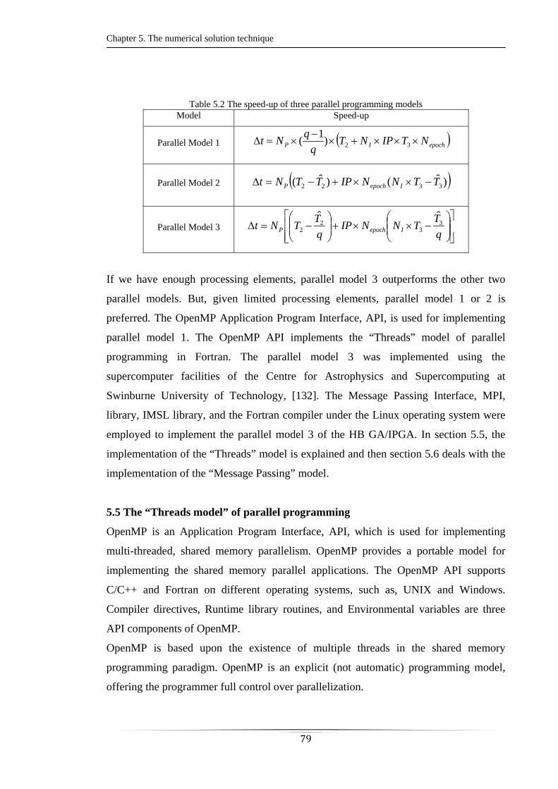
Chapter 5. The numerical solution technique
79
Table 5.2 The speed-up of three parallel programming models Model Speed-up
Parallel Model 1 epochIP NTIPNTq
qNt
32)
1(
Parallel Model 2 )ˆ()ˆ( 3322 TTNNIPTTNt IepochP
Parallel Model 3
q
TTNNIP
q
TTNt IepochP
33
22
ˆˆ
If we have enough processing elements, parallel model 3 outperforms the other two
parallel models. But, given limited processing elements, parallel model 1 or 2 is
preferred. The OpenMP Application Program Interface, API, is used for implementing
parallel model 1. The OpenMP API implements the “Threads” model of parallel
programming in Fortran. The parallel model 3 was implemented using the
supercomputer facilities of the Centre for Astrophysics and Supercomputing at
Swinburne University of Technology, [132]. The Message Passing Interface, MPI,
library, IMSL library, and the Fortran compiler under the Linux operating system were
employed to implement the parallel model 3 of the HB GA/IPGA. In section 5.5, the
implementation of the “Threads” model is explained and then section 5.6 deals with the
implementation of the “Message Passing” model.
5.5 The “Threads model” of parallel programming
OpenMP is an Application Program Interface, API, which is used for implementing
multi-threaded, shared memory parallelism. OpenMP provides a portable model for
implementing the shared memory parallel applications. The OpenMP API supports
C/C++ and Fortran on different operating systems, such as, UNIX and Windows.
Compiler directives, Runtime library routines, and Environmental variables are three
API components of OpenMP.
OpenMP is based upon the existence of multiple threads in the shared memory
programming paradigm. OpenMP is an explicit (not automatic) programming model,
offering the programmer full control over parallelization.
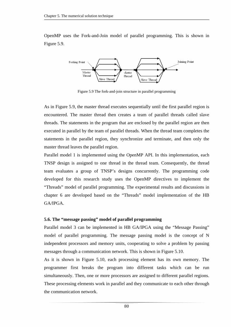
Chapter 5. The numerical solution technique
80
OpenMP uses the Fork-and-Join model of parallel programming. This is shown in
Figure 5.9.
Figure 5.9 The fork-and-join structure in parallel programming
As in Figure 5.9, the master thread executes sequentially until the first parallel region is
encountered. The master thread then creates a team of parallel threads called slave
threads. The statements in the program that are enclosed by the parallel region are then
executed in parallel by the team of parallel threads. When the thread team completes the
statements in the parallel region, they synchronize and terminate, and then only the
master thread leaves the parallel region.
Parallel model 1 is implemented using the OpenMP API. In this implementation, each
TNSP design is assigned to one thread in the thread team. Consequently, the thread
team evaluates a group of TNSP’s designs concurrently. The programming code
developed for this research study uses the OpenMP directives to implement the
“Threads” model of parallel programming. The experimental results and discussions in
chapter 6 are developed based on the “Threads” model implementation of the HB
GA/IPGA.
5.6. The “message passing” model of parallel programming
Parallel model 3 can be implemented in HB GA/IPGA using the “Message Passing”
model of parallel programming. The message passing model is the concept of N
independent processors and memory units, cooperating to solve a problem by passing
messages through a communication network. This is shown in Figure 5.10.
As it is shown in Figure 5.10, each processing element has its own memory. The
programmer first breaks the program into different tasks which can be run
simultaneously. Then, one or more processors are assigned to different parallel regions.
These processing elements work in parallel and they communicate to each other through
the communication network.
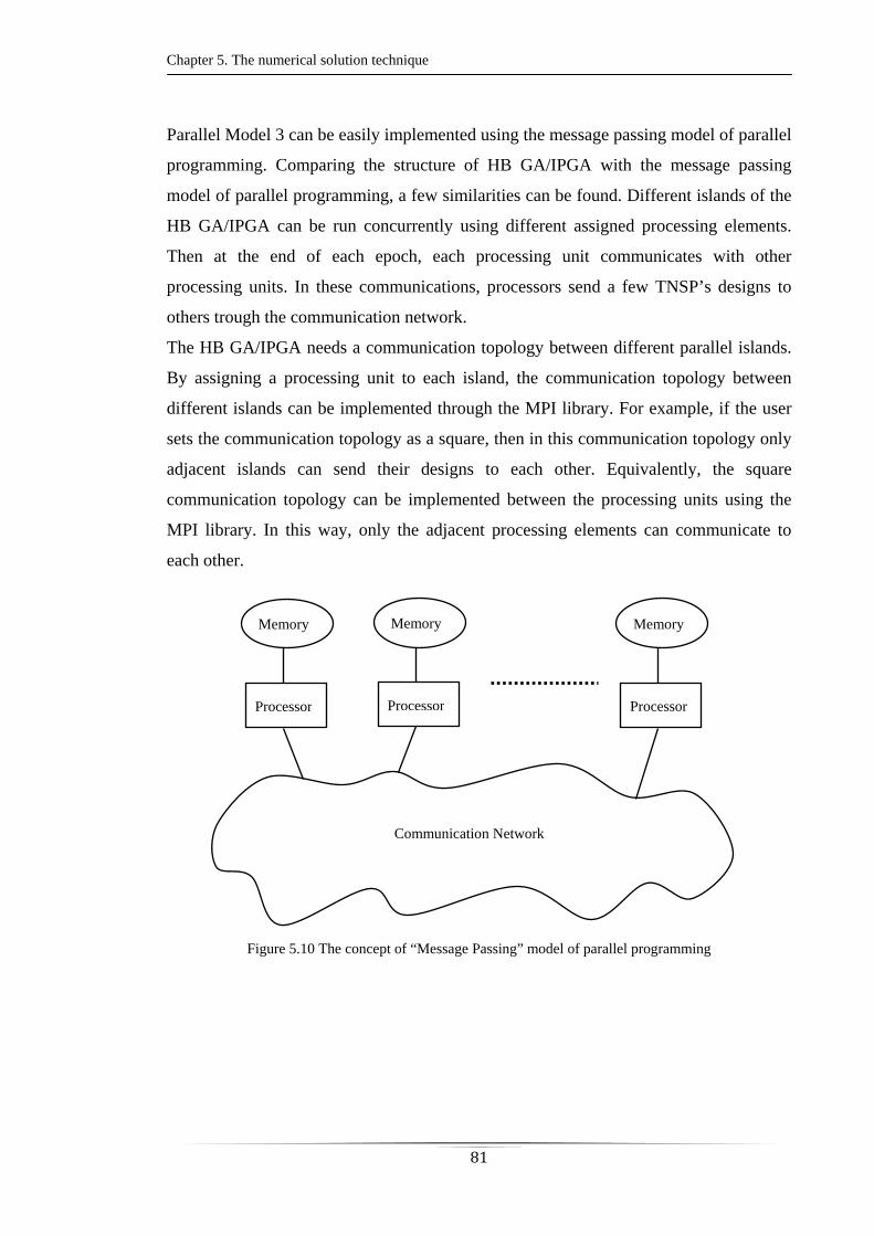
Chapter 5. The numerical solution technique
81
Parallel Model 3 can be easily implemented using the message passing model of parallel
programming. Comparing the structure of HB GA/IPGA with the message passing
model of parallel programming, a few similarities can be found. Different islands of the
HB GA/IPGA can be run concurrently using different assigned processing elements.
Then at the end of each epoch, each processing unit communicates with other
processing units. In these communications, processors send a few TNSP’s designs to
others trough the communication network.
The HB GA/IPGA needs a communication topology between different parallel islands.
By assigning a processing unit to each island, the communication topology between
different islands can be implemented through the MPI library. For example, if the user
sets the communication topology as a square, then in this communication topology only
adjacent islands can send their designs to each other. Equivalently, the square
communication topology can be implemented between the processing units using the
MPI library. In this way, only the adjacent processing elements can communicate to
each other.
Figure 5.10 The concept of “Message Passing” model of parallel programming
Communication Network
Memory
Processor
Memory
Processor
Memory
Processor
Chapter 5. The numerical solution technique
82
5.7 Chapter summary
This chapter develops a numerical solution termed a Hybrid Bilevel Genetic
Algorithm/Island Parallel Genetic Algorithm, HB GA/IPGA, to solve the derived
mathematical structures in chapter 4. The HB GA/IPGA has two levels. The GA deals
with the TNSP’s decision variables and the IPGA deals with the bidding behaviors of
the rival GenCos participating in the electricity market. The IPGA module uses the
concept of parallel islands to find the set of Nash equilibriums of the electricity market.
In doing so, each island explores the set of possible bids of the GenCos independently.
A stability operator is developed to determine whether or not an island is stabilized. If it
is stabilized, then the island is used again for finding the Nash equilibriums of rival
GenCos. To improve the efficiency of the developed HB GA/IPGA, high performance
computing techniques are used. Given the structure of the HB GA/IPGA, three parallel
programming models are designed. Model 1 of parallel programming focuses on
running the GA part of the HB GA/IPGA in parallel. Model 2 focuses on computing the
IPGA in parallel. Finally, design 3 parallelizes both the GA part and the IPGA part of
the HB GA/IPGA.
The “Threads” model of parallel programming is used for implementing model 1. In the
threads model, a master thread executes the program until it encounters a parallel
region. Then, the master thread forms a group of threads and the group of threads runs
the parallel region. At the end of parallel region, the master thread leaves the parallel
region.
The OpenMP application program interface embedded in Fortran was employed in
developing the programming code of the HB GA/IPGA.
The “Message Passing” model of parallel programming is used for implementing model
3. In the message passing implementations, different processing elements are assigned
to different parallel tasks. These processing elements run their assigned tasks in parallel
and they communicate to each other through the communication network. The MPI
library and Fortran compiler installed on the Linux operating system were used for
developing the programming code of the HB GA/IPGA.

CHAPTER 6 – EXPERIMENTAL RESULTS
Chapter 6. Experimental results
84
6.1 Introduction
This chapter discusses experimental results of the optimisation problems set out in
chapter 4 for the assessment of a transmission augmentation. Section 6.2 covers
approaches 1 and 2 from chapter 4. These two approaches are discussed and compared
to each other. Section 6.3 deals with the approach based on the concept of social
welfare. The strategic generation investment of GenCos and the interaction of the
generation investment and transmission investment are studied and discussed in section
6.4. In section 6.4, approach 4 is compared with the approach 3 and the traditional
approach to transmission augmentation. Finally, section 6.5 concludes this chapter.
6.2 Experimental results of approaches 1 and 2 to transmission augmentation
In this section two example power systems are selected and analysed. The modified
Garver’s example system is used to illustrate and explore the proposed approaches.
Further, the IEEE 14-bus example system is modified and employed to illustrate the
process of analysis of a transmission system augmentation including the numerical
solution technique. Both example systems are designed carefully to suit the needs of the
economic studies. Throughout the economic study, we compare the optimal policies of
the TNSP obtained by the proposed optimisation problems (4.14) and (4.16) with each
other. Also, the optimal policy of a TNSP in the absence of market power is compared
with the results of the problems in (4.14) and (4.16). An implementation of the proposed
numerical solution technique is written in the Fortran language using the International
Mathematical and Statistical Library, IMSL. The developed code is solved on a double
core, 3.0GHz , Pentium-4 PC.
6.2.1 The modified Garver’s example system
For conceptual evaluation of the proposed approaches, a modified Garver’s Six-Bus
example system has been tested, [135].
The Garver’s example system has been modified to a network with six buses and eight
transmission lines. The key data of the system is presented in Table 6.1 through Table
6.4.
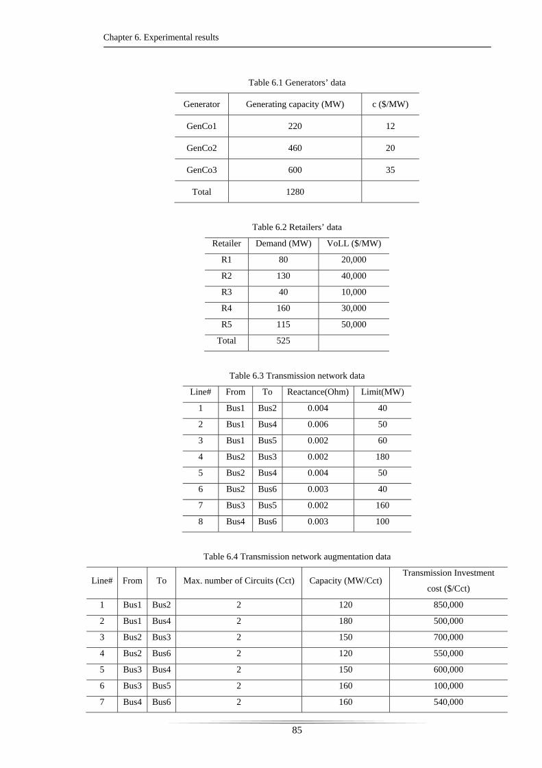
Chapter 6. Experimental results
85
Table 6.1 Generators’ data
Generator Generating capacity (MW) c ($/MW)
GenCo1 220 12
GenCo2 460 20
GenCo3 600 35
Total 1280
Table 6.2 Retailers’ data
Retailer Demand (MW) VoLL ($/MW)
R1 80 20,000
R2 130 40,000
R3 40 10,000
R4 160 30,000
R5 115 50,000
Total 525
Table 6.3 Transmission network data
Line# From To Reactance(Ohm) Limit(MW)
1 Bus1 Bus2 0.004 40
2 Bus1 Bus4 0.006 50
3 Bus1 Bus5 0.002 60
4 Bus2 Bus3 0.002 180
5 Bus2 Bus4 0.004 50
6 Bus2 Bus6 0.003 40
7 Bus3 Bus5 0.002 160
8 Bus4 Bus6 0.003 100
Table 6.4 Transmission network augmentation data
Line# From To Max. number of Circuits (Cct) Capacity (MW/Cct) Transmission Investment
cost ($/Cct)
1 Bus1 Bus2 2 120 850,000
2 Bus1 Bus4 2 180 500,000
3 Bus2 Bus3 2 150 700,000
4 Bus2 Bus6 2 120 550,000
5 Bus3 Bus4 2 150 600,000
6 Bus3 Bus5 2 160 100,000
7 Bus4 Bus6 2 160 540,000
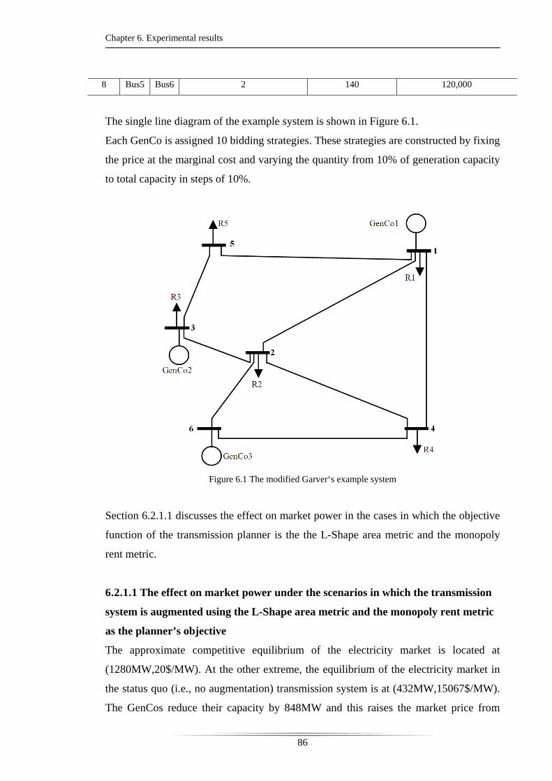
Chapter 6. Experimental results
86
8 Bus5 Bus6 2 140 120,000
The single line diagram of the example system is shown in Figure 6.1.
Each GenCo is assigned 10 bidding strategies. These strategies are constructed by fixing
the price at the marginal cost and varying the quantity from 10% of generation capacity
to total capacity in steps of 10%.
Figure 6.1 The modified Garver‘s example system
Section 6.2.1.1 discusses the effect on market power in the cases in which the objective
function of the transmission planner is the the L-Shape area metric and the monopoly
rent metric.
6.2.1.1 The effect on market power under the scenarios in which the transmission
system is augmented using the L-Shape area metric and the monopoly rent metric
as the planner’s objective
The approximate competitive equilibrium of the electricity market is located at
(1280MW,20$/MW). At the other extreme, the equilibrium of the electricity market in
the status quo (i.e., no augmentation) transmission system is at (432MW,15067$/MW).
The GenCos reduce their capacity by 848MW and this raises the market price from
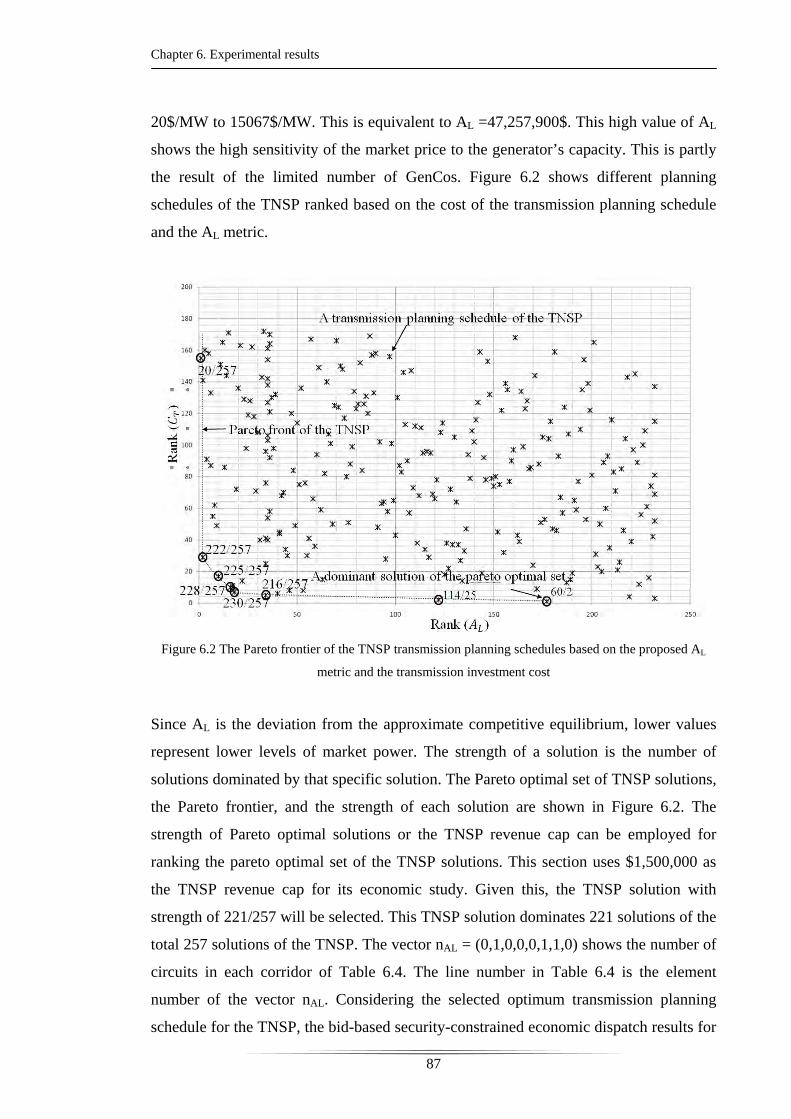
Chapter 6. Experimental results
87
20$/MW to 15067$/MW. This is equivalent to AL =47,257,900$. This high value of AL
shows the high sensitivity of the market price to the generator’s capacity. This is partly
the result of the limited number of GenCos. Figure 6.2 shows different planning
schedules of the TNSP ranked based on the cost of the transmission planning schedule
and the AL metric.
Figure 6.2 The Pareto frontier of the TNSP transmission planning schedules based on the proposed AL
metric and the transmission investment cost
Since AL is the deviation from the approximate competitive equilibrium, lower values
represent lower levels of market power. The strength of a solution is the number of
solutions dominated by that specific solution. The Pareto optimal set of TNSP solutions,
the Pareto frontier, and the strength of each solution are shown in Figure 6.2. The
strength of Pareto optimal solutions or the TNSP revenue cap can be employed for
ranking the pareto optimal set of the TNSP solutions. This section uses $1,500,000 as
the TNSP revenue cap for its economic study. Given this, the TNSP solution with
strength of 221/257 will be selected. This TNSP solution dominates 221 solutions of the
total 257 solutions of the TNSP. The vector nAL = (0,1,0,0,0,1,1,0) shows the number of
circuits in each corridor of Table 6.4. The line number in Table 6.4 is the element
number of the vector nAL. Considering the selected optimum transmission planning
schedule for the TNSP, the bid-based security-constrained economic dispatch results for

Chapter 6. Experimental results
88
the equilibrium of the electricity market in status quo transmission system and in
augmented transmission system are collected in Table 6.5 through Table 6.8.
Table 6.9 compares the market power metrics of financial withholding, physical
withholding, and the proposed AL metric in two scenarios of the status quo transmission
system and the augmented transmission system. The overall profit of GenCos is
calculated in the last row of Table 6.9.
As in Table 6.9, the transmission planning schedule nAL has decreased the market power
in terms of financial withholding by 46%. This is measured by price distortion metric,
ΔPriceDistortion. Similarly, quantity withheld measured by ΔQuantityWithheld has reduced
by 6% which is an improvement in overall physical withholding.
Table 6.5 Economic dispatch results in the equilibrium of the electricity market in status quo transmission
system
Bus
No. Voltage Angle (radian) Generation (MW) Load (MW) LP* ($/MWh)
1 0.00 220.00 73.33 20,000
2 -0.16 0.00 106.00 40,000
3 -0.05 92.00 0.00 45,000
4 -0.28 0.00 156.67 30,000
5 -0.12 0.00 96.00 50,000
6 -0.04 120.00 0.00 27,500
Total/Installed 432/432 432/525
Average of Nodal Prices($/MWh) 35,416
LP* : Locational Price
Table 6.6 Power flows of the transmission lines in the equilibrium of the electricity market in status quo
transmission system
From To Power Flow(MW) Capacity (MW)
Bus1 Bus2 40.00(Congested) 40.00
Bus1 Bus4 46.67 50.00
Bus1 Bus5 60.00(Congested) 60.00
Bus2 Bus3 -56.00 180.00
Bus2 Bus4 30.00 50.00
Bus2 Bus6 -40.00(Congested) 40.00
Bus3 Bus5 36.00 160.00
Bus4 Bus6 -80.00 100.00
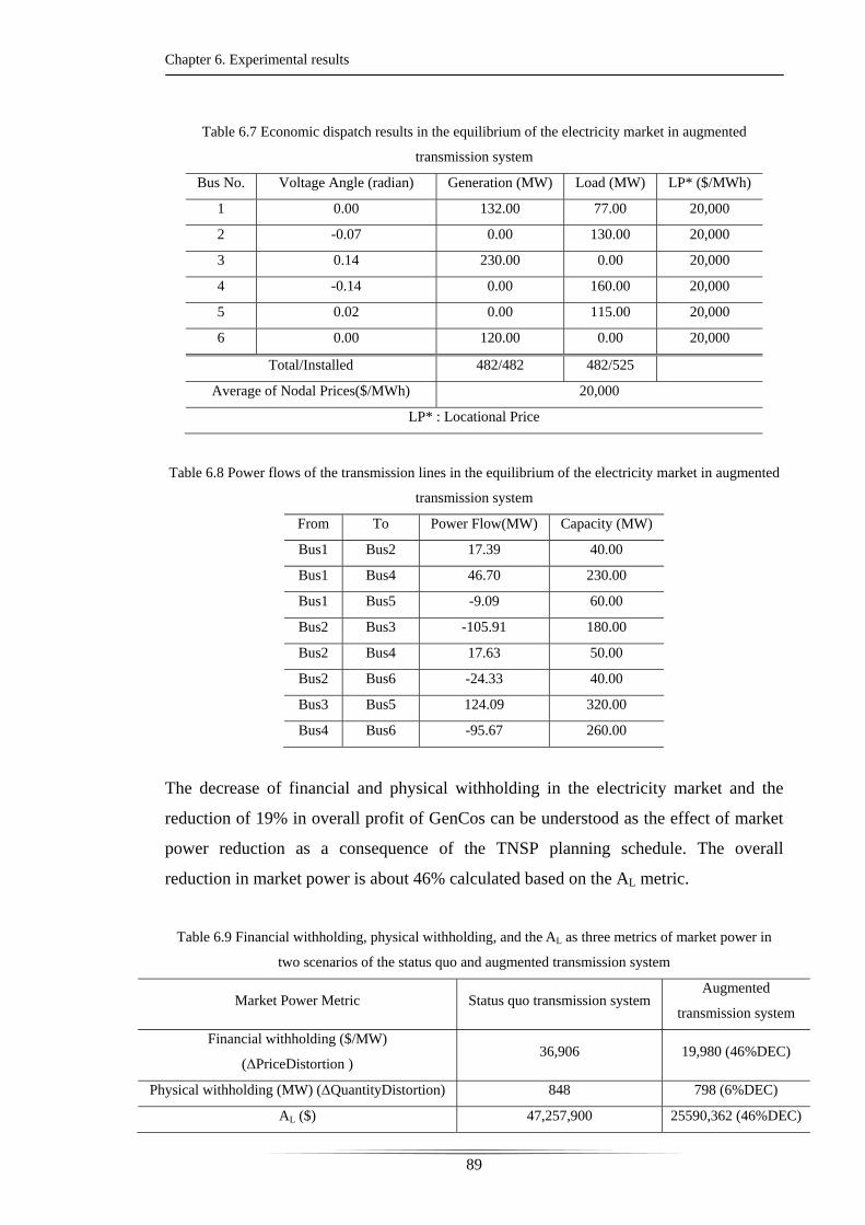
Chapter 6. Experimental results
89
Table 6.7 Economic dispatch results in the equilibrium of the electricity market in augmented
transmission system
Bus No. Voltage Angle (radian) Generation (MW) Load (MW) LP* ($/MWh)
1 0.00 132.00 77.00 20,000
2 -0.07 0.00 130.00 20,000
3 0.14 230.00 0.00 20,000
4 -0.14 0.00 160.00 20,000
5 0.02 0.00 115.00 20,000
6 0.00 120.00 0.00 20,000
Total/Installed 482/482 482/525
Average of Nodal Prices($/MWh) 20,000
LP* : Locational Price
Table 6.8 Power flows of the transmission lines in the equilibrium of the electricity market in augmented
transmission system
From To Power Flow(MW) Capacity (MW)
Bus1 Bus2 17.39 40.00
Bus1 Bus4 46.70 230.00
Bus1 Bus5 -9.09 60.00
Bus2 Bus3 -105.91 180.00
Bus2 Bus4 17.63 50.00
Bus2 Bus6 -24.33 40.00
Bus3 Bus5 124.09 320.00
Bus4 Bus6 -95.67 260.00
The decrease of financial and physical withholding in the electricity market and the
reduction of 19% in overall profit of GenCos can be understood as the effect of market
power reduction as a consequence of the TNSP planning schedule. The overall
reduction in market power is about 46% calculated based on the AL metric.
Table 6.9 Financial withholding, physical withholding, and the AL as three metrics of market power in
two scenarios of the status quo and augmented transmission system
Market Power Metric Status quo transmission system Augmented
transmission system
Financial withholding ($/MW)
(ΔPriceDistortion ) 36,906 19,980 (46%DEC)
Physical withholding (MW) (ΔQuantityDistortion) 848 798 (6%DEC)
AL ($) 47,257,900 25590,362 (46%DEC)

Chapter 6. Experimental results
90
Overall profit of GenCos 11,831,320 9,629,616 (19%DEC)
INC : Increase DEC : Decrease
While the transmission planning schedule nAL = (0,1,0,0,0,1,1,0) reduces the market
power of the electricity market, the traditional mechanism for transmission
augmentation as formulated in (4.24) does not approve any transmission augmentation
in this example system.
Figure 6.3 shows offer curves of the GenCos in the two scenarios of the status quo and
augmented transmission systems. Note that as a result of the augmentation, GenCo2
offers more of its capacity, which has an impact on GenCo 1 withholding some of its
capacity.
Table 6.10 shows the GenCos’ profits in the two scenarios of the status quo and
augmented transmission system.
If we solve the mathematical structure in (4.14) using the numerical solution approach
in chapter 5, the Pareto frontier of the TNSP transmission planning schedules would
result in a three-dimensional figure as shown in Figure 6.4.
The Pareto frontier has 28 different planning schedules of the TNSP. These planning
schedules are dominant alternative solutions of the TNSP for economic augmentation of
the transmission system. Using $1,500,000 as the TNSP revenue cap and ranking the
Pareto frontier solutions, results in the vector nMR = (0,1,0,0,0,1,1,0) being chosen as the
TNSP solution.
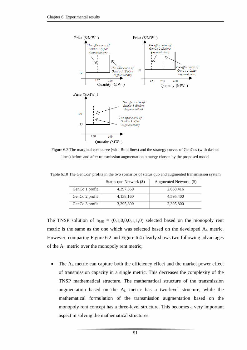
Chapter 6. Experimental results
91
Figure 6.3 The marginal cost curve (with Bold lines) and the strategy curves of GenCos (with dashed
lines) before and after transmission augmentation strategy chosen by the proposed model
Table 6.10 The GenCos’ profits in the two scenarios of status quo and augmented transmission system
Status quo Network ($) Augmented Network, ($)
GenCo 1 profit 4,397,360 2,638,416
GenCo 2 profit 4,138,160 4,595,400
GenCo 3 profit 3,295,800 2,395,800
The TNSP solution of nMR = (0,1,0,0,0,1,1,0) selected based on the monopoly rent
metric is the same as the one which was selected based on the developed AL metric.
However, comparing Figure 6.2 and Figure 6.4 clearly shows two following advantages
of the AL metric over the monopoly rent metric;
The AL metric can capture both the efficiency effect and the market power effect
of transmission capacity in a single metric. This decreases the complexity of the
TNSP mathematical structure. The mathematical structure of the transmission
augmentation based on the AL metric has a two-level structure, while the
mathematical formulation of the transmission augmentation based on the
monopoly rent concept has a three-level structure. This becomes a very important
aspect in solving the mathematical structures.
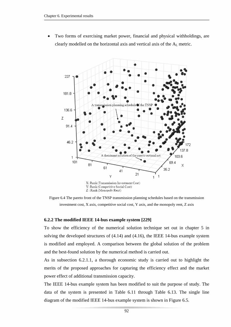
Chapter 6. Experimental results
92
Two forms of exercising market power, financial and physical withholdings, are
clearly modelled on the horizontal axis and vertical axis of the AL metric.
Figure 6.4 The pareto front of the TNSP transmission planning schedules based on the transmission
investment cost, X axis, competitive social cost, Y axis, and the monopoly rent, Z axis
6.2.2 The modified IEEE 14-bus example system [229]
To show the efficiency of the numerical solution technique set out in chapter 5 in
solving the developed structures of (4.14) and (4.16), the IEEE 14-bus example system
is modified and employed. A comparison between the global solution of the problem
and the best-found solution by the numerical method is carried out.
As in subsection 6.2.1.1, a thorough economic study is carried out to highlight the
merits of the proposed approaches for capturing the efficiency effect and the market
power effect of additional transmission capacity.
The IEEE 14-bus example system has been modified to suit the purpose of study. The
data of the system is presented in Table 6.11 through Table 6.13. The single line
diagram of the modified IEEE 14-bus example system is shown in Figure 6.5.
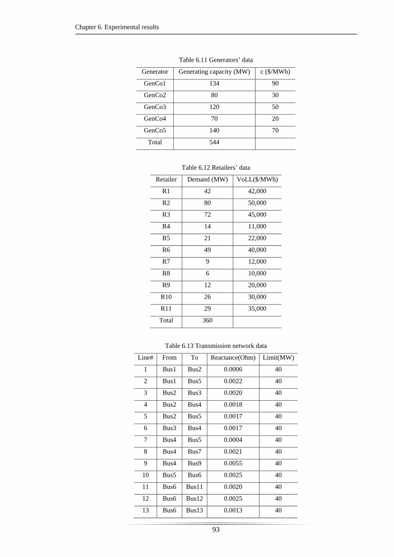
Chapter 6. Experimental results
93
Table 6.11 Generators’ data
Generator Generating capacity (MW) c ($/MWh)
GenCo1 134 90
GenCo2 80 30
GenCo3 120 50
GenCo4 70 20
GenCo5 140 70
Total 544
Table 6.12 Retailers’ data
Retailer Demand (MW) VoLL($/MWh)
R1 42 42,000
R2 80 50,000
R3 72 45,000
R4 14 11,000
R5 21 22,000
R6 49 40,000
R7 9 12,000
R8 6 10,000
R9 12 20,000
R10 26 30,000
R11 29 35,000
Total 360
Table 6.13 Transmission network data
Line# From To Reactance(Ohm) Limit(MW)
1 Bus1 Bus2 0.0006 40
2 Bus1 Bus5 0.0022 40
3 Bus2 Bus3 0.0020 40
4 Bus2 Bus4 0.0018 40
5 Bus2 Bus5 0.0017 40
6 Bus3 Bus4 0.0017 40
7 Bus4 Bus5 0.0004 40
8 Bus4 Bus7 0.0021 40
9 Bus4 Bus9 0.0055 40
10 Bus5 Bus6 0.0025 40
11 Bus6 Bus11 0.0020 40
12 Bus6 Bus12 0.0025 40
13 Bus6 Bus13 0.0013 40
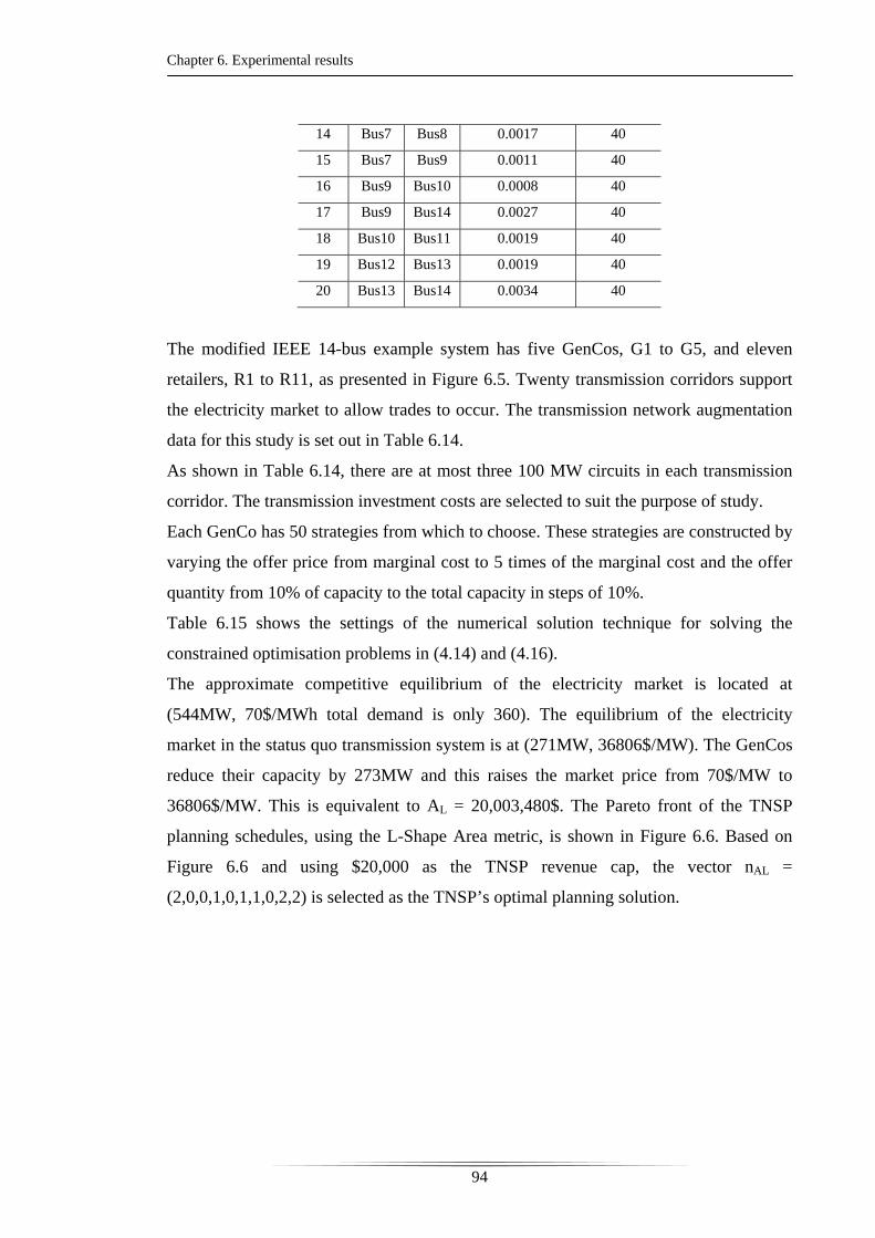
Chapter 6. Experimental results
94
14 Bus7 Bus8 0.0017 40
15 Bus7 Bus9 0.0011 40
16 Bus9 Bus10 0.0008 40
17 Bus9 Bus14 0.0027 40
18 Bus10 Bus11 0.0019 40
19 Bus12 Bus13 0.0019 40
20 Bus13 Bus14 0.0034 40
The modified IEEE 14-bus example system has five GenCos, G1 to G5, and eleven
retailers, R1 to R11, as presented in Figure 6.5. Twenty transmission corridors support
the electricity market to allow trades to occur. The transmission network augmentation
data for this study is set out in Table 6.14.
As shown in Table 6.14, there are at most three 100 MW circuits in each transmission
corridor. The transmission investment costs are selected to suit the purpose of study.
Each GenCo has 50 strategies from which to choose. These strategies are constructed by
varying the offer price from marginal cost to 5 times of the marginal cost and the offer
quantity from 10% of capacity to the total capacity in steps of 10%.
Table 6.15 shows the settings of the numerical solution technique for solving the
constrained optimisation problems in (4.14) and (4.16).
The approximate competitive equilibrium of the electricity market is located at
(544MW, 70$/MWh total demand is only 360). The equilibrium of the electricity
market in the status quo transmission system is at (271MW, 36806$/MW). The GenCos
reduce their capacity by 273MW and this raises the market price from 70$/MW to
36806$/MW. This is equivalent to AL = 20,003,480$. The Pareto front of the TNSP
planning schedules, using the L-Shape Area metric, is shown in Figure 6.6. Based on
Figure 6.6 and using $20,000 as the TNSP revenue cap, the vector nAL =
(2,0,0,1,0,1,1,0,2,2) is selected as the TNSP’s optimal planning solution.
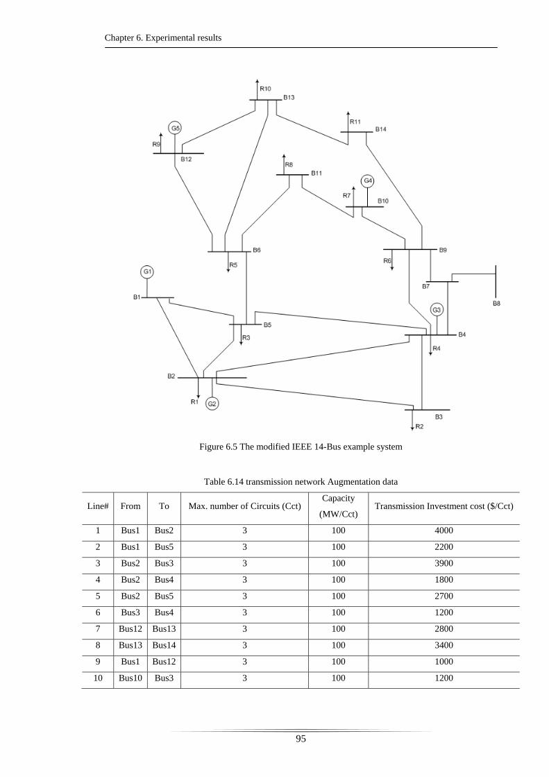
Chapter 6. Experimental results
95
Figure 6.5 The modified IEEE 14-Bus example system
Table 6.14 transmission network Augmentation data
Line# From To Max. number of Circuits (Cct) Capacity
(MW/Cct) Transmission Investment cost ($/Cct)
1 Bus1 Bus2 3 100 4000
2 Bus1 Bus5 3 100 2200
3 Bus2 Bus3 3 100 3900
4 Bus2 Bus4 3 100 1800
5 Bus2 Bus5 3 100 2700
6 Bus3 Bus4 3 100 1200
7 Bus12 Bus13 3 100 2800
8 Bus13 Bus14 3 100 3400
9 Bus1 Bus12 3 100 1000
10 Bus10 Bus3 3 100 1200
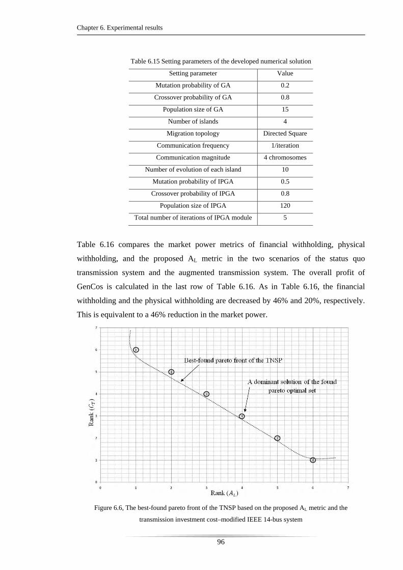
Chapter 6. Experimental results
96
Table 6.15 Setting parameters of the developed numerical solution
Setting parameter Value
Mutation probability of GA 0.2
Crossover probability of GA 0.8
Population size of GA 15
Number of islands 4
Migration topology Directed Square
Communication frequency 1/iteration
Communication magnitude 4 chromosomes
Number of evolution of each island 10
Mutation probability of IPGA 0.5
Crossover probability of IPGA 0.8
Population size of IPGA 120
Total number of iterations of IPGA module 5
Table 6.16 compares the market power metrics of financial withholding, physical
withholding, and the proposed AL metric in the two scenarios of the status quo
transmission system and the augmented transmission system. The overall profit of
GenCos is calculated in the last row of Table 6.16. As in Table 6.16, the financial
withholding and the physical withholding are decreased by 46% and 20%, respectively.
This is equivalent to a 46% reduction in the market power.
Figure 6.6, The best-found pareto front of the TNSP based on the proposed AL metric and the
transmission investment cost–modified IEEE 14-bus system
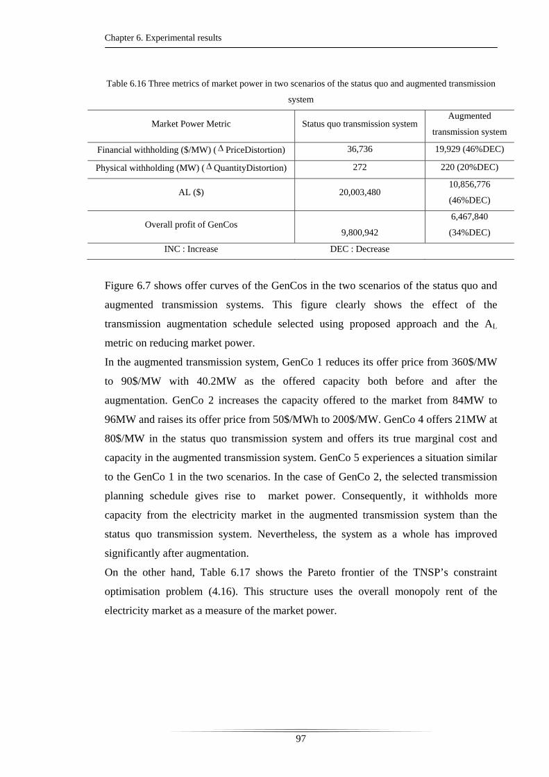
Chapter 6. Experimental results
97
Table 6.16 Three metrics of market power in two scenarios of the status quo and augmented transmission
system
Market Power Metric Status quo transmission system Augmented
transmission system
Financial withholding ($/MW) ( PriceDistortion) 36,736 19,929 (46%DEC)
Physical withholding (MW) ( QuantityDistortion) 272 220 (20%DEC)
AL ($) 20,003,480 10,856,776
(46%DEC)
Overall profit of GenCos 9,800,942
6,467,840
(34%DEC)
INC : Increase DEC : Decrease
Figure 6.7 shows offer curves of the GenCos in the two scenarios of the status quo and
augmented transmission systems. This figure clearly shows the effect of the
transmission augmentation schedule selected using proposed approach and the AL
metric on reducing market power.
In the augmented transmission system, GenCo 1 reduces its offer price from 360$/MW
to 90$/MW with 40.2MW as the offered capacity both before and after the
augmentation. GenCo 2 increases the capacity offered to the market from 84MW to
96MW and raises its offer price from 50$/MWh to 200$/MW. GenCo 4 offers 21MW at
80$/MW in the status quo transmission system and offers its true marginal cost and
capacity in the augmented transmission system. GenCo 5 experiences a situation similar
to the GenCo 1 in the two scenarios. In the case of GenCo 2, the selected transmission
planning schedule gives rise to market power. Consequently, it withholds more
capacity from the electricity market in the augmented transmission system than the
status quo transmission system. Nevertheless, the system as a whole has improved
significantly after augmentation.
On the other hand, Table 6.17 shows the Pareto frontier of the TNSP’s constraint
optimisation problem (4.16). This structure uses the overall monopoly rent of the
electricity market as a measure of the market power.
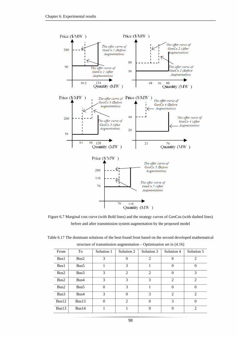
Chapter 6. Experimental results
98
Figure 6.7 Marginal cost curve (with Bold lines) and the strategy curves of GenCos (with dashed lines)
before and after transmission system augmentation by the proposed model
Table 6.17 The dominant solutions of the best-found front based on the second developed mathematical
structure of transmission augmentation – Optimisation set in (4.16)
From To Solution 1 Solution 2 Solution 3 Solution 4 Solution 5
Bus1 Bus2 3 0 2 0 2
Bus1 Bus5 1 3 1 0 0
Bus2 Bus3 3 2 2 0 3
Bus2 Bus4 3 3 3 2 2
Bus2 Bus5 0 3 1 0 0
Bus3 Bus4 3 0 3 2 2
Bus12 Bus13 0 2 0 3 0
Bus13 Bus14 1 1 0 0 2
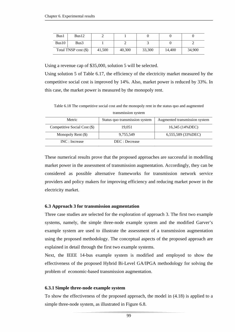
Chapter 6. Experimental results
99
Bus1 Bus12 2 1 0 0 0
Bus10 Bus3 1 2 3 0 2
Total TNSP cost ($) 41,500 40,300 33,300 14,400 34,900
Using a revenue cap of $35,000, solution 5 will be selected.
Using solution 5 of Table 6.17, the efficiency of the electricity market measured by the
competitive social cost is improved by 14%. Also, market power is reduced by 33%. In
this case, the market power is measured by the monopoly rent.
Table 6.18 The competitive social cost and the monopoly rent in the status quo and augmented
transmission system
Metric Status quo transmission system Augmented transmission system
Competitive Social Cost ($) 19,051 16,345 (14%DEC)
Monopoly Rent ($) 9,755,549 6,555,589 (33%DEC)
INC : Increase DEC : Decrease
These numerical results prove that the proposed approaches are successful in modelling
market power in the assessment of transmission augmentation. Accordingly, they can be
considered as possible alternative frameworks for transmission network service
providers and policy makers for improving efficiency and reducing market power in the
electricity market.
6.3 Approach 3 for transmission augmentation
Three case studies are selected for the exploration of approach 3. The first two example
systems, namely, the simple three-node example system and the modified Garver’s
example system are used to illustrate the assessment of a transmission augmentation
using the proposed methodology. The conceptual aspects of the proposed approach are
explained in detail through the first two example systems.
Next, the IEEE 14-bus example system is modified and employed to show the
effectiveness of the proposed Hybrid Bi-Level GA/IPGA methodology for solving the
problem of economic-based transmission augmentation.
6.3.1 Simple three-node example system
To show the effectiveness of the proposed approach, the model in (4.18) is applied to a
simple three-node system, as illustrated in Figure 6.8.
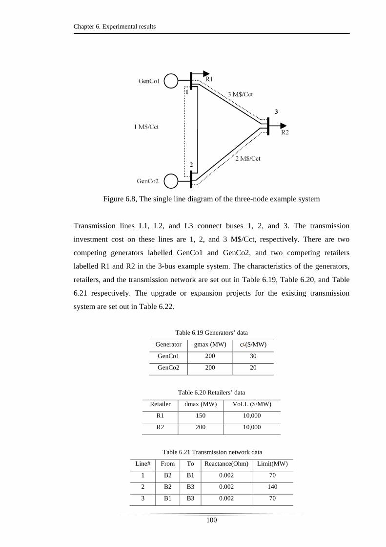
Chapter 6. Experimental results
100
Figure 6.8, The single line diagram of the three-node example system
Transmission lines L1, L2, and L3 connect buses 1, 2, and 3. The transmission
investment cost on these lines are 1, 2, and 3 M$/Cct, respectively. There are two
competing generators labelled GenCo1 and GenCo2, and two competing retailers
labelled R1 and R2 in the 3-bus example system. The characteristics of the generators,
retailers, and the transmission network are set out in Table 6.19, Table 6.20, and Table
6.21 respectively. The upgrade or expansion projects for the existing transmission
system are set out in Table 6.22.
Table 6.19 Generators’ data
Generator gmax (MW) c ($/MW)
GenCo1 200 30
GenCo2 200 20
Table 6.20 Retailers’ data
Retailer dmax (MW) VoLL ($/MW)
R1 150 10,000
R2 200 10,000
Table 6.21 Transmission network data
Line# From To Reactance(Ohm) Limit(MW)
1 B2 B1 0.002 70
2 B2 B3 0.002 140
3 B1 B3 0.002 70
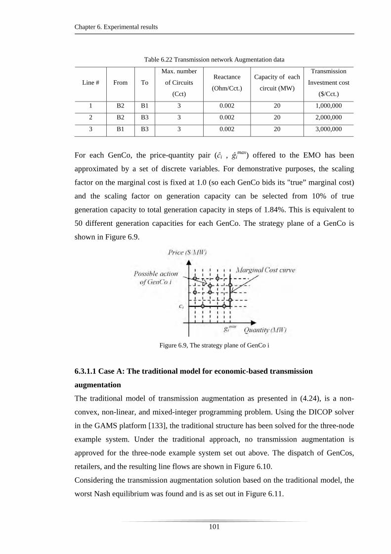
Chapter 6. Experimental results
101
Table 6.22 Transmission network Augmentation data
Line # From To
Max. number
of Circuits
(Cct)
Reactance
(Ohm/Cct.)
Capacity of each
circuit (MW)
Transmission
Investment cost
($/Cct.)
1 B2 B1 3 0.002 20 1,000,000
2 B2 B3 3 0.002 20 2,000,000
3 B1 B3 3 0.002 20 3,000,000
For each GenCo, the price-quantity pair (ĉi , ĝimax) offered to the EMO has been
approximated by a set of discrete variables. For demonstrative purposes, the scaling
factor on the marginal cost is fixed at 1.0 (so each GenCo bids its "true” marginal cost)
and the scaling factor on generation capacity can be selected from 10% of true
generation capacity to total generation capacity in steps of 1.84%. This is equivalent to
50 different generation capacities for each GenCo. The strategy plane of a GenCo is
shown in Figure 6.9.
Figure 6.9, The strategy plane of GenCo i
6.3.1.1 Case A: The traditional model for economic-based transmission
augmentation
The traditional model of transmission augmentation as presented in (4.24), is a non-
convex, non-linear, and mixed-integer programming problem. Using the DICOP solver
in the GAMS platform [133], the traditional structure has been solved for the three-node
example system. Under the traditional approach, no transmission augmentation is
approved for the three-node example system set out above. The dispatch of GenCos,
retailers, and the resulting line flows are shown in Figure 6.10.
Considering the transmission augmentation solution based on the traditional model, the
worst Nash equilibrium was found and is as set out in Figure 6.11.
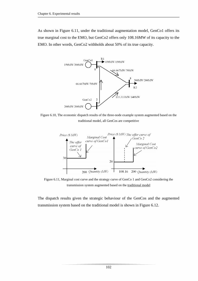
Chapter 6. Experimental results
102
As shown in Figure 6.11, under the traditional augmentation model, GenCo1 offers its
true marginal cost to the EMO, but GenCo2 offers only 108.16MW of its capacity to the
EMO. In other words, GenCo2 withholds about 50% of its true capacity.
Figure 6.10, The economic dispatch results of the three-node example system augmented based on the
traditional model, all GenCos are competitive
Figure 6.11, Marginal cost curve and the strategy curve of GenCo 1 and GenCo2 considering the
transmission system augmented based on the traditional model
The dispatch results given the strategic behaviour of the GenCos and the augmented
transmission system based on the traditional model is shown in Figure 6.12.

Chapter 6. Experimental results
103
Figure 6.12, The economic dispatch results of the three-node example system augmented based on the
traditional model, GenCos behave strategically
Under the traditional model of augmentation, the total transmission investment cost is
$0.0 and the social cost found based on the worst Nash equilibrium and the weighting
factor of σ=10.0 is $4,294,592.
6.3.1.2 Case B: The proposed model for economically-efficient transmission
augmentation
The proposed model in (4.18) has been used to determine an economically-efficient
transmission augmentation. This time the algorithm approves the building of a 20MW
circuit between nodes 2 and 3. The worst Nash equilibrium of GenCo1 and GenCo2
considering the 20MW augmentation of transmission system is found and is as
indicated in Figure 6.13.
As is clear from Figure 6.13, the additional 20 MW augmentation encourages GenCo2
to behave more competitively.
Figure 6.13, Marginal cost curve and the strategy curve of GenCo 1 and GenCo2 considering the
transmission system augmented based on the proposed model
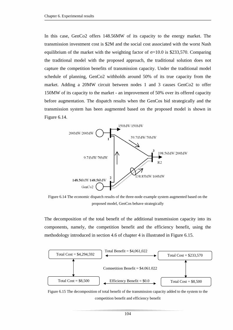
Chapter 6. Experimental results
104
In this case, GenCo2 offers 148.56MW of its capacity to the energy market. The
transmission investment cost is $2M and the social cost associated with the worst Nash
equilibrium of the market with the weighting factor of σ=10.0 is $233,570. Comparing
the traditional model with the proposed approach, the traditional solution does not
capture the competition benefits of transmission capacity. Under the traditional model
schedule of planning, GenCo2 withholds around 50% of its true capacity from the
market. Adding a 20MW circuit between nodes 1 and 3 causes GenCo2 to offer
150MW of its capacity to the market - an improvement of 50% over its offered capacity
before augmentation. The dispatch results when the GenCos bid strategically and the
transmission system has been augmented based on the proposed model is shown in
Figure 6.14.
Figure 6.14 The economic dispatch results of the three-node example system augmented based on the
proposed model, GenCos behave strategically
The decomposition of the total benefit of the additional transmission capacity into its
components, namely, the competition benefit and the efficiency benefit, using the
methodology introduced in section 4.6 of chapter 4 is illustrated in Figure 6.15.
Figure 6.15 The decomposition of total benefit of the transmission capacity added to the system to the
competition benefit and efficiency benefit
Total Cost = $4,294,592 Total Cost = $233,570
Total Cost = $8,500
Total Benefit = $4,061,022
Competition Benefit = $4,061,022
Total Cost = $8,500 Efficiency Benefit = $0.0

Chapter 6. Experimental results
105
In fact, as shown in Figure 6.15, the additional transmission capacity between buses 2
and 3 only has value for improving competition between generators and does not have
any traditional efficiency benefit.
6.3.2 Modified Garver’s six-bus example system
For further conceptual evaluation of the developed structure, a modified Garver’s Six-
Bus example system has been tested.
Garver’s example system has been modified to reflect a network with six buses and
eight transmission lines. The key parameters of the system are presented in Table 6.23
through Table 6.26.
Table 6.23 Generators’ data
Generator gmax (MW) c ($/MW)
GenCo1 220 12
GenCo2 460 20
GenCo3 600 35
Total 1280
Table 6.24 Retailers’ data
Retailer dmax (MW) VoLL ($/MW)
R1 80 20,000
R2 130 40,000
R3 40 10,000
R4 160 30,000
R5 115 50,000
Total 525
Table 6.25 Transmission network data
Line# From To Reactance
(Ohm.) Limit(MW)
1 Bus1 Bus2 0.004 40
2 Bus1 Bus4 0.006 50
3 Bus1 Bus5 0.002 60
4 Bus2 Bus3 0.002 180
5 Bus2 Bus4 0.004 50
6 Bus2 Bus6 0.003 40
7 Bus3 Bus5 0.002 160
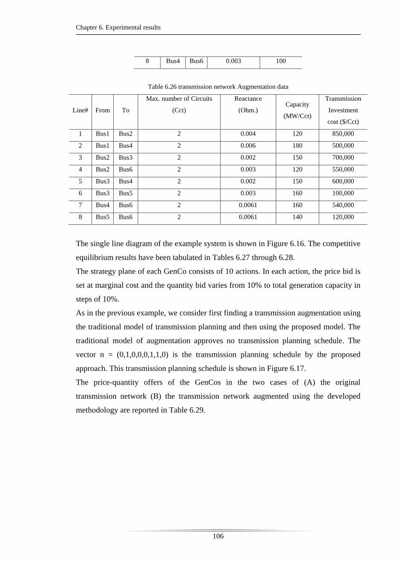
Chapter 6. Experimental results
106
8 Bus4 Bus6 0.003 100
Table 6.26 transmission network Augmentation data
Line# From To
Max. number of Circuits
(Cct)
Reactance
(Ohm.) Capacity
(MW/Cct)
Transmission
Investment
cost ($/Cct)
1 Bus1 Bus2 2 0.004 120 850,000
2 Bus1 Bus4 2 0.006 180 500,000
3 Bus2 Bus3 2 0.002 150 700,000
4 Bus2 Bus6 2 0.003 120 550,000
5 Bus3 Bus4 2 0.002 150 600,000
6 Bus3 Bus5 2 0.003 160 100,000
7 Bus4 Bus6 2 0.0061 160 540,000
8 Bus5 Bus6 2 0.0061 140 120,000
The single line diagram of the example system is shown in Figure 6.16. The competitive
equilibrium results have been tabulated in Tables 6.27 through 6.28.
The strategy plane of each GenCo consists of 10 actions. In each action, the price bid is
set at marginal cost and the quantity bid varies from 10% to total generation capacity in
steps of 10%.
As in the previous example, we consider first finding a transmission augmentation using
the traditional model of transmission planning and then using the proposed model. The
traditional model of augmentation approves no transmission planning schedule. The
vector n = (0,1,0,0,0,1,1,0) is the transmission planning schedule by the proposed
approach. This transmission planning schedule is shown in Figure 6.17.
The price-quantity offers of the GenCos in the two cases of (A) the original
transmission network (B) the transmission network augmented using the developed
methodology are reported in Table 6.29.

Chapter 6. Experimental results
107
Figure 6.16, The modified Garver‘s example system
Table 6.27 economic dispatch results under competitive equilibrium condition
Bus
No. Voltage Angle (degree) Generation (MW) Load (MW) CLP* ($/MWh)
1 0.00 156.67 80.00 12.00
2 -5.73 - 130.00 24.00
3 12.80 315.00 40.00 20.00
4 -17.19 - 160.00 46.00
5 -0.19 - 115.00 16.00
6 -6.88 53.33 - 35.00
Total/Installed 525/1280 525/525
Average of Nodal Prices($/MWh) 25.50
Total Generation Cost ($/h) 10046.67
Total Value of Lost Load($/h) 0.0
CLP* : Competitive Locational Price
Table 6.28 economic dispatch results for existing transmission lines under competitive equilibrium
condition
From To Power Flow(MW)
Bus1 Bus2 25.00
Bus1 Bus4 50.00(congested)
Bus1 Bus5 1.67

Chapter 6. Experimental results
108
Bus2 Bus3 -161.67
Bus2 Bus4 50.00(congested)
Bus2 Bus6 6.67
Bus3 Bus5 113.33
Bus4 Bus6 -60.00
As in Table 6.29, the total offered capacity, the total withheld capacity, and HHI have
been improved by 11.57%, 6%, and 4.50% respectively.
As shown in Table 6.29, the proposed approach results in a significantly lower total
social cost than the traditional approach. Figure 6.18 illustrates the use of the
methodology introduced in section 4.6 of chapter 4 to decompose the total benefit of the
proposed augmentations into the competition benefit and the efficiency benefit.
Figure 6.17 The modified Garver ‘s example system augmented by the traditional method (no
augmentation) and proposed method (dashed lines)
Table 6.29 The price-quantity outcomes of GenCos 1, 2, 3 found based on the worst Nash equilibrium
Original Network - Augmented
Network,
traditional approach
Augmented Network,
proposed approach
GenCo 1 ($/MWh,MW) (12,220) (12,132)
GenCo 2 ($/MWh,MW) (20,92) (20,230)
GenCo 3 ($/MWh,MW) (35,120) (35,120)
Total offered capacity(MW) 432 482
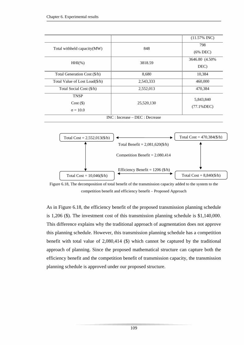
Chapter 6. Experimental results
109
(11.57% INC)
Total withheld capacity(MW) 848 798
(6% DEC)
HHI(%) 3818.59 3646.80 (4.50%
DEC)
Total Generation Cost ($/h) 8,680 10,384
Total Value of Lost Load($/h) 2,543,333 460,000
Total Social Cost ($/h) 2,552,013 470,384
TNSP
Cost ($)
σ = 10.0
25,520,130 5,843,840
(77.1%DEC)
INC : Increase – DEC : Decrease
Figure 6.18, The decomposition of total benefit of the transmission capacity added to the system to the
competition benefit and efficiency benefit – Proposed Approach
As in Figure 6.18, the efficiency benefit of the proposed transmission planning schedule
is 1,206 ($). The investment cost of this transmission planning schedule is $1,140,000.
This difference explains why the traditional approach of augmentation does not approve
this planning schedule. However, this transmission planning schedule has a competition
benefit with total value of 2,080,414 ($) which cannot be captured by the traditional
approach of planning. Since the proposed mathematical structure can capture both the
efficiency benefit and the competition benefit of transmission capacity, the transmission
planning schedule is approved under our proposed structure.
Total Cost = 2,552,013($/h) Total Cost = 470,384($/h)
Total Cost = 10,046($/h)
Total Benefit = 2,081,620($/h)
Competition Benefit = 2,080,414
Total Cost = 8,840($/h)Efficiency Benefit = 1206 ($/h)
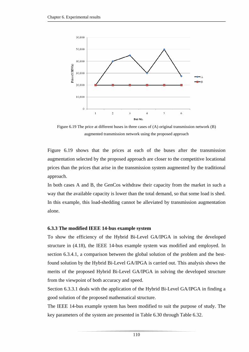
Chapter 6. Experimental results
110
Figure 6.19 The price at different buses in three cases of (A) original transmission network (B)
augmented transmission network using the proposed approach
Figure 6.19 shows that the prices at each of the buses after the transmission
augmentation selected by the proposed approach are closer to the competitive locational
prices than the prices that arise in the transmission system augmented by the traditional
approach.
In both cases A and B, the GenCos withdraw their capacity from the market in such a
way that the available capacity is lower than the total demand, so that some load is shed.
In this example, this load-shedding cannot be alleviated by transmission augmentation
alone.
6.3.3 The modified IEEE 14-bus example system
To show the efficiency of the Hybrid Bi-Level GA/IPGA in solving the developed
structure in (4.18), the IEEE 14-bus example system was modified and employed. In
section 6.3.4.1, a comparison between the global solution of the problem and the best-
found solution by the Hybrid Bi-Level GA/IPGA is carried out. This analysis shows the
merits of the proposed Hybrid Bi-Level GA/IPGA in solving the developed structure
from the viewpoint of both accuracy and speed.
Section 6.3.3.1 deals with the application of the Hybrid Bi-Level GA/IPGA in finding a
good solution of the proposed mathematical structure.
The IEEE 14-bus example system has been modified to suit the purpose of study. The
key parameters of the system are presented in Table 6.30 through Table 6.32.
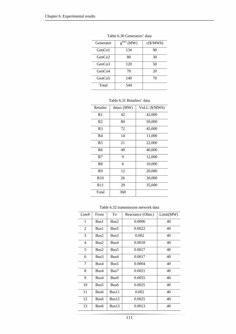
Chapter 6. Experimental results
111
Table 6.30 Generators’ data
Generator gmax (MW) c($/MWh)
GenCo1 134 90
GenCo2 80 30
GenCo3 120 50
GenCo4 70 20
GenCo5 140 70
Total 544
Table 6.31 Retailers’ data
Retailer dmax (MW) VoLL ($/MWh)
R1 42 42,000
R2 80 50,000
R3 72 45,000
R4 14 11,000
R5 21 22,000
R6 49 40,000
R7 9 12,000
R8 6 10,000
R9 12 20,000
R10 26 30,000
R11 29 35,000
Total 360
Table 6.32 transmission network data
Line# From To Reactance (Ohm.) Limit(MW)
1 Bus1 Bus2 0.0006 40
2 Bus1 Bus5 0.0022 40
3 Bus2 Bus3 0.002 40
4 Bus2 Bus4 0.0018 40
5 Bus2 Bus5 0.0017 40
6 Bus3 Bus4 0.0017 40
7 Bus4 Bus5 0.0004 40
8 Bus4 Bus7 0.0021 40
9 Bus4 Bus9 0.0055 40
10 Bus5 Bus6 0.0025 40
11 Bus6 Bus11 0.002 40
12 Bus6 Bus12 0.0025 40
13 Bus6 Bus13 0.0013 40
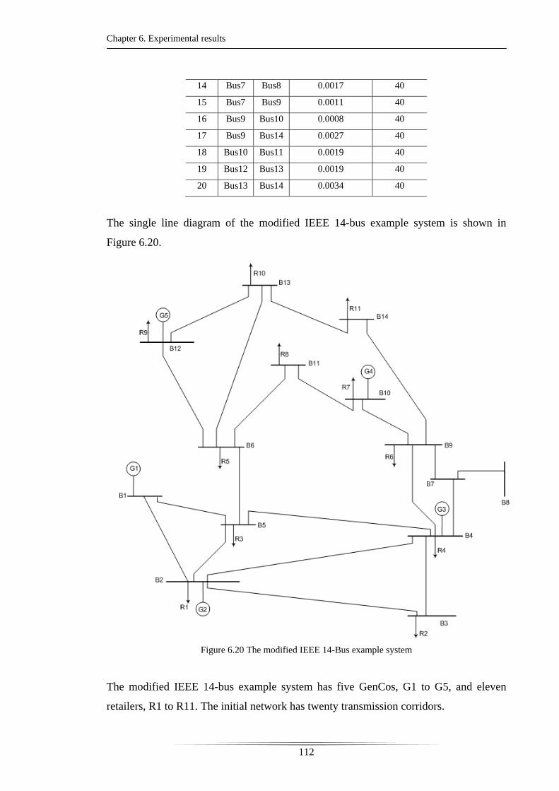
Chapter 6. Experimental results
112
14 Bus7 Bus8 0.0017 40
15 Bus7 Bus9 0.0011 40
16 Bus9 Bus10 0.0008 40
17 Bus9 Bus14 0.0027 40
18 Bus10 Bus11 0.0019 40
19 Bus12 Bus13 0.0019 40
20 Bus13 Bus14 0.0034 40
The single line diagram of the modified IEEE 14-bus example system is shown in
Figure 6.20.
Figure 6.20 The modified IEEE 14-Bus example system
The modified IEEE 14-bus example system has five GenCos, G1 to G5, and eleven
retailers, R1 to R11. The initial network has twenty transmission corridors.

Chapter 6. Experimental results
113
6.3.3.1 The Hybrid Bi-level GA/IPGA parameters and its performance
The transmission network augmentation data for this study is illustrated in Table 6.33.
The lines indicated by a star in this table are used only for the section 6.3.3.2 study.
Table 6.33 Transmission network Augmentation data
Line# From To
Max. number of
Circuits (Cct)
Reactance (Ohm.) Capacity
(MW/Cct)
Transmission
Investment
cost ($/Cct)
1 Bus1 Bus2 1 0.0006 100 4000
2 Bus1 Bus5 1 0.0022 100 2200
3 Bus2 Bus3 1 0.0019 100 3900
4 Bus2 Bus4 1 0.0018 100 1800
5 Bus2 Bus5 1 0.0017 100 2700
6 Bus3 Bus4 1 0.0012 100 1200
7 Bus12 Bus13 1 0.0011 100 2800
8 Bus13 Bus14 1 0.0034 100 3400
9* Bus1 Bus12 1 0.0002 100 1000
10* Bus10 Bus3 1 0.0002 100 1200
The strategy plane of each GenCo consists of 8 actions. These actions all involve
offering the generator’s output at marginal cost with the quantity bid varying from 30%
to total generation capacity in steps of 10%. The retailers are assumed to be fully
competitive.
Using the enumeration technique, the global optimum of the developed structure in
(4.18) is located at (1,1,0,0,1,1,1,0) with TNSP’s total cost equal to $6,981,547. The
Hybrid Bi-Level GA/IPGA has been used with the parameters set out in Table 6.34.
Table 6.34 Parameters of the Hybrid Bi-level GA/IPGA used for section 6.3.4.1 study
Parameter Value
Mutation probability of GA 0.2
Crossover probability of GA 0.8
Population size of GA 15
Number of islands 4
Migration topology Directed Square
Communication frequency 1/iteration
Communication magnitude 4 chromosomes
Number of evolution of each island 12
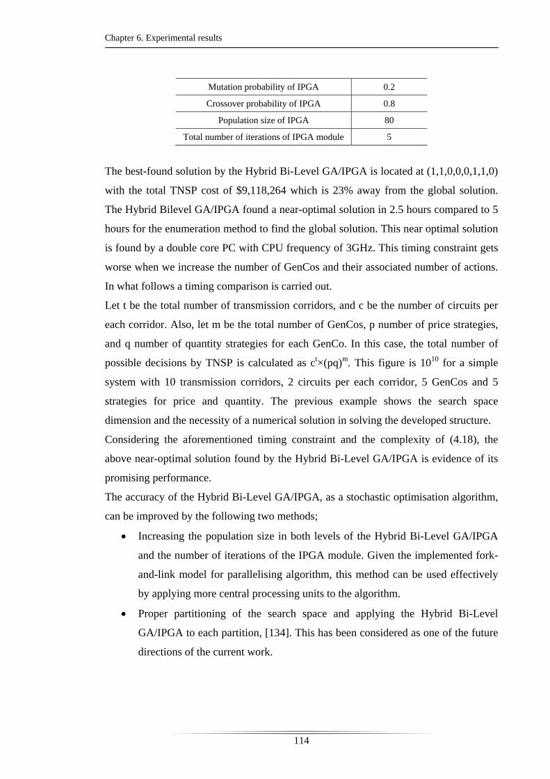
Chapter 6. Experimental results
114
Mutation probability of IPGA 0.2
Crossover probability of IPGA 0.8
Population size of IPGA 80
Total number of iterations of IPGA module 5
The best-found solution by the Hybrid Bi-Level GA/IPGA is located at (1,1,0,0,0,1,1,0)
with the total TNSP cost of $9,118,264 which is 23% away from the global solution.
The Hybrid Bilevel GA/IPGA found a near-optimal solution in 2.5 hours compared to 5
hours for the enumeration method to find the global solution. This near optimal solution
is found by a double core PC with CPU frequency of 3GHz. This timing constraint gets
worse when we increase the number of GenCos and their associated number of actions.
In what follows a timing comparison is carried out.
Let t be the total number of transmission corridors, and c be the number of circuits per
each corridor. Also, let m be the total number of GenCos, p number of price strategies,
and q number of quantity strategies for each GenCo. In this case, the total number of
possible decisions by TNSP is calculated as ct×(pq)m. This figure is 1010 for a simple
system with 10 transmission corridors, 2 circuits per each corridor, 5 GenCos and 5
strategies for price and quantity. The previous example shows the search space
dimension and the necessity of a numerical solution in solving the developed structure.
Considering the aforementioned timing constraint and the complexity of (4.18), the
above near-optimal solution found by the Hybrid Bi-Level GA/IPGA is evidence of its
promising performance.
The accuracy of the Hybrid Bi-Level GA/IPGA, as a stochastic optimisation algorithm,
can be improved by the following two methods;
Increasing the population size in both levels of the Hybrid Bi-Level GA/IPGA
and the number of iterations of the IPGA module. Given the implemented fork-
and-link model for parallelising algorithm, this method can be used effectively
by applying more central processing units to the algorithm.
Proper partitioning of the search space and applying the Hybrid Bi-Level
GA/IPGA to each partition, [134]. This has been considered as one of the future
directions of the current work.
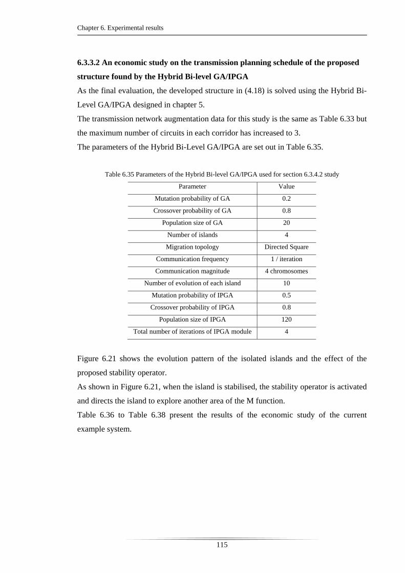
Chapter 6. Experimental results
115
6.3.3.2 An economic study on the transmission planning schedule of the proposed
structure found by the Hybrid Bi-level GA/IPGA
As the final evaluation, the developed structure in (4.18) is solved using the Hybrid Bi-
Level GA/IPGA designed in chapter 5.
The transmission network augmentation data for this study is the same as Table 6.33 but
the maximum number of circuits in each corridor has increased to 3.
The parameters of the Hybrid Bi-Level GA/IPGA are set out in Table 6.35.
Table 6.35 Parameters of the Hybrid Bi-level GA/IPGA used for section 6.3.4.2 study
Parameter Value
Mutation probability of GA 0.2
Crossover probability of GA 0.8
Population size of GA 20
Number of islands 4
Migration topology Directed Square
Communication frequency 1 / iteration
Communication magnitude 4 chromosomes
Number of evolution of each island 10
Mutation probability of IPGA 0.5
Crossover probability of IPGA 0.8
Population size of IPGA 120
Total number of iterations of IPGA module 4
Figure 6.21 shows the evolution pattern of the isolated islands and the effect of the
proposed stability operator.
As shown in Figure 6.21, when the island is stabilised, the stability operator is activated
and directs the island to explore another area of the M function.
Table 6.36 to Table 6.38 present the results of the economic study of the current
example system.
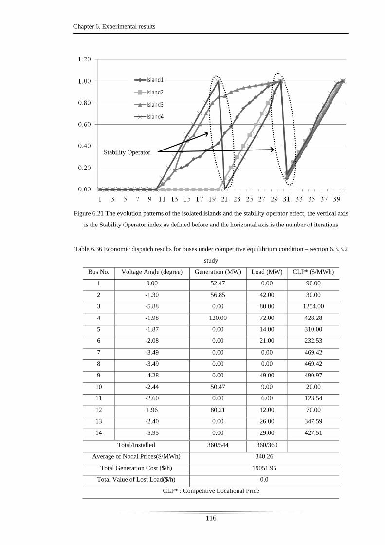
Chapter 6. Experimental results
116
Figure 6.21 The evolution patterns of the isolated islands and the stability operator effect, the vertical axis
is the Stability Operator index as defined before and the horizontal axis is the number of iterations
Table 6.36 Economic dispatch results for buses under competitive equilibrium condition – section 6.3.3.2
study
Bus No. Voltage Angle (degree) Generation (MW) Load (MW) CLP* ($/MWh)
1 0.00 52.47 0.00 90.00
2 -1.30 56.85 42.00 30.00
3 -5.88 0.00 80.00 1254.00
4 -1.98 120.00 72.00 428.28
5 -1.87 0.00 14.00 310.00
6 -2.08 0.00 21.00 232.53
7 -3.49 0.00 0.00 469.42
8 -3.49 0.00 0.00 469.42
9 -4.28 0.00 49.00 490.97
10 -2.44 50.47 9.00 20.00
11 -2.60 0.00 6.00 123.54
12 1.96 80.21 12.00 70.00
13 -2.40 0.00 26.00 347.59
14 -5.95 0.00 29.00 427.51
Total/Installed 360/544 360/360
Average of Nodal Prices($/MWh) 340.26
Total Generation Cost ($/h) 19051.95
Total Value of Lost Load($/h) 0.0
CLP* : Competitive Locational Price
Stability Operator
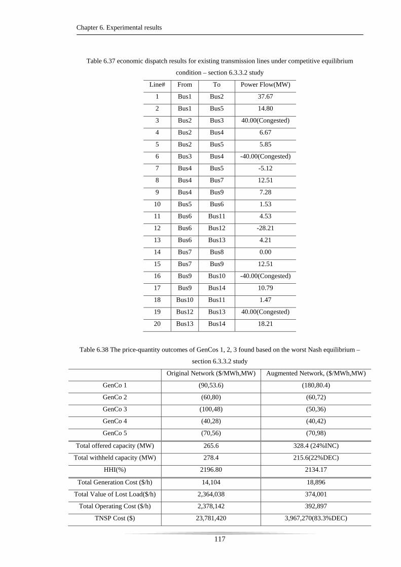
Chapter 6. Experimental results
117
Table 6.37 economic dispatch results for existing transmission lines under competitive equilibrium
condition – section 6.3.3.2 study
Line# From To Power Flow(MW)
1 Bus1 Bus2 37.67
2 Bus1 Bus5 14.80
3 Bus2 Bus3 40.00(Congested)
4 Bus2 Bus4 6.67
5 Bus2 Bus5 5.85
6 Bus3 Bus4 -40.00(Congested)
7 Bus4 Bus5 -5.12
8 Bus4 Bus7 12.51
9 Bus4 Bus9 7.28
10 Bus5 Bus6 1.53
11 Bus6 Bus11 4.53
12 Bus6 Bus12 -28.21
13 Bus6 Bus13 4.21
14 Bus7 Bus8 0.00
15 Bus7 Bus9 12.51
16 Bus9 Bus10 -40.00(Congested)
17 Bus9 Bus14 10.79
18 Bus10 Bus11 1.47
19 Bus12 Bus13 40.00(Congested)
20 Bus13 Bus14 18.21
Table 6.38 The price-quantity outcomes of GenCos 1, 2, 3 found based on the worst Nash equilibrium –
section 6.3.3.2 study
Original Network ($/MWh,MW) Augmented Network, ($/MWh,MW)
GenCo 1 (90,53.6) (180,80.4)
GenCo 2 (60,80) (60,72)
GenCo 3 (100,48) (50,36)
GenCo 4 (40,28) (40,42)
GenCo 5 (70,56) (70,98)
Total offered capacity (MW) 265.6 328.4 (24%INC)
Total withheld capacity (MW) 278.4 215.6(22%DEC)
HHI(%) 2196.80 2134.17
Total Generation Cost ($/h) 14,104 18,896
Total Value of Lost Load($/h) 2,364,038 374,001
Total Operating Cost ($/h) 2,378,142 392,897
TNSP Cost ($) 23,781,420 3,967,270(83.3%DEC)

Chapter 6. Experimental results
118
σ = 10.0
INC : Increase – DEC : Decrease
Solving the proposed structure for economic-based transmission augmentation using the
Hybrid Bilevel GA/IPGA results in the vector (3,2,3,1,0,1,1,0,2,2) as the TNSP’s
planning schedule. As set out in Table 6.38, the planning schedule decreases the
withheld capacity of the GenCos by 22%. This causes a decrease of 83.3% in the total
social cost. The market benefit of this transmission planning schedule with a
decomposition of the total benefit to the efficiency benefit and competition benefit is set
out in Figure 6.22.
Figure 6.22 Decomposition of total benefit of the additional transmission capacity to the competition
benefit and efficiency benefit – section 6.3.3.2 study
The GenCos’ offer curves before and after augmentation and their competitive strategy
is shown in Figure 6.23.
As is clear from Figure 6.23, the transmission planning strategy has significantly
changed the bidding behaviour of the GenCos in the electricity market.
Table 6.39 shows GenCos’ profit in three scenarios, namely, the competitive bidding
scenario, the strategic bidding scenario before augmentation, and the strategic bidding
scenario after augmentation.
The calculation of the Monopoly Rent, MR, is a further indicator that the transmission
planning schedule resulting from the proposed methodology has increased competition
in the generation sector.
Total Cost = 2,378,142($/h) Total Cost = 392,897($/h)
Total Cost = 19,051($/h)
Total Benefit = 1,985,245($/h)
Competition Benefit = 1,982,294($/h)
Total Cost = 16,100 ($/h)Efficiency Benefit = 2951($/h)
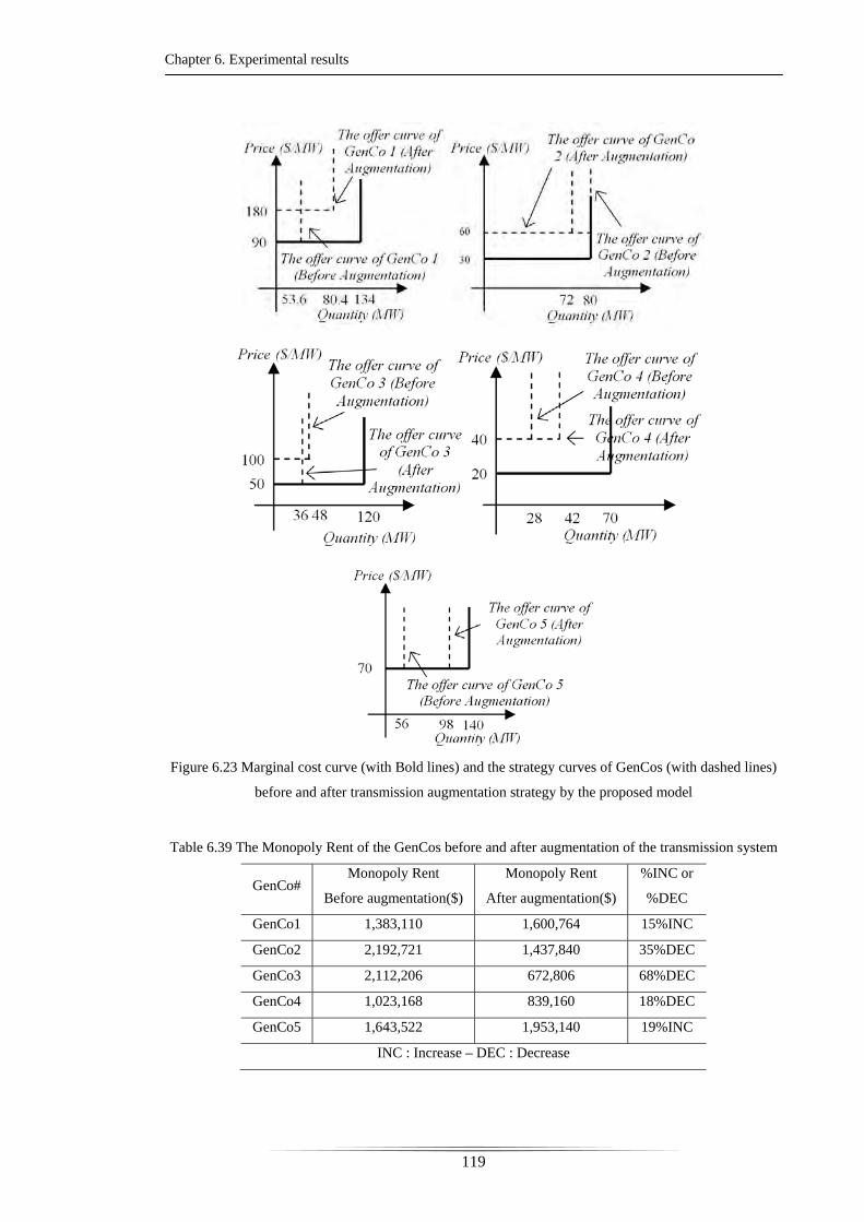
Chapter 6. Experimental results
119
Figure 6.23 Marginal cost curve (with Bold lines) and the strategy curves of GenCos (with dashed lines)
before and after transmission augmentation strategy by the proposed model
Table 6.39 The Monopoly Rent of the GenCos before and after augmentation of the transmission system
GenCo# Monopoly Rent
Before augmentation($)
Monopoly Rent
After augmentation($)
%INC or
%DEC
GenCo1 1,383,110 1,600,764 15%INC
GenCo2 2,192,721 1,437,840 35%DEC
GenCo3 2,112,206 672,806 68%DEC
GenCo4 1,023,168 839,160 18%DEC
GenCo5 1,643,522 1,953,140 19%INC
INC : Increase – DEC : Decrease
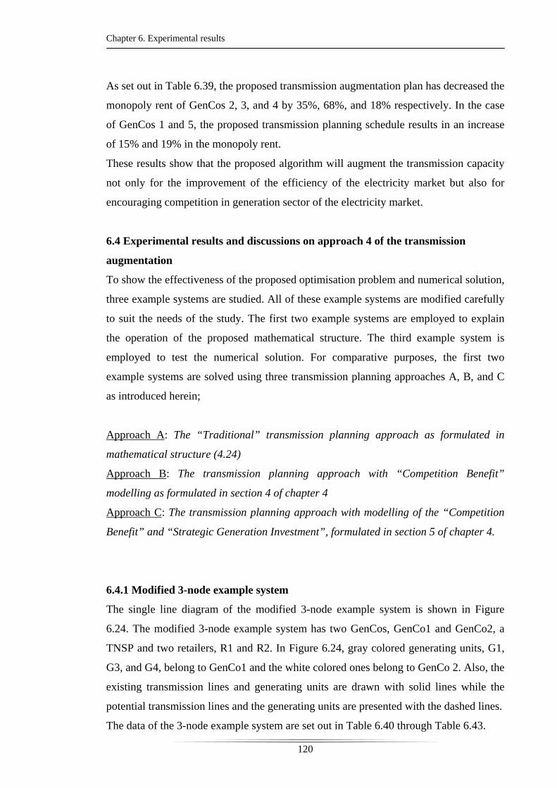
Chapter 6. Experimental results
120
As set out in Table 6.39, the proposed transmission augmentation plan has decreased the
monopoly rent of GenCos 2, 3, and 4 by 35%, 68%, and 18% respectively. In the case
of GenCos 1 and 5, the proposed transmission planning schedule results in an increase
of 15% and 19% in the monopoly rent.
These results show that the proposed algorithm will augment the transmission capacity
not only for the improvement of the efficiency of the electricity market but also for
encouraging competition in generation sector of the electricity market.
6.4 Experimental results and discussions on approach 4 of the transmission
augmentation
To show the effectiveness of the proposed optimisation problem and numerical solution,
three example systems are studied. All of these example systems are modified carefully
to suit the needs of the study. The first two example systems are employed to explain
the operation of the proposed mathematical structure. The third example system is
employed to test the numerical solution. For comparative purposes, the first two
example systems are solved using three transmission planning approaches A, B, and C
as introduced herein;
Approach A: The “Traditional” transmission planning approach as formulated in
mathematical structure (4.24)
Approach B: The transmission planning approach with “Competition Benefit”
modelling as formulated in section 4 of chapter 4
Approach C: The transmission planning approach with modelling of the “Competition
Benefit” and “Strategic Generation Investment”, formulated in section 5 of chapter 4.
6.4.1 Modified 3-node example system
The single line diagram of the modified 3-node example system is shown in Figure
6.24. The modified 3-node example system has two GenCos, GenCo1 and GenCo2, a
TNSP and two retailers, R1 and R2. In Figure 6.24, gray colored generating units, G1,
G3, and G4, belong to GenCo1 and the white colored ones belong to GenCo 2. Also, the
existing transmission lines and generating units are drawn with solid lines while the
potential transmission lines and the generating units are presented with the dashed lines.
The data of the 3-node example system are set out in Table 6.40 through Table 6.43.
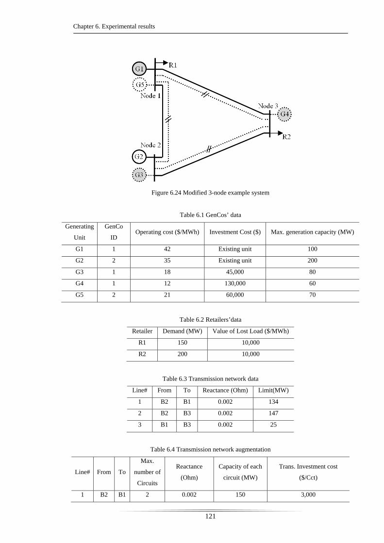
Chapter 6. Experimental results
121
Figure 6.24 Modified 3-node example system
Table 6.1 GenCos’ data
Generating
Unit
GenCo
ID Operating cost ($/MWh) Investment Cost ($) Max. generation capacity (MW)
G1 1 42 Existing unit 100
G2 2 35 Existing unit 200
G3 1 18 45,000 80
G4 1 12 130,000 60
G5 2 21 60,000 70
Table 6.2 Retailers’data
Retailer Demand (MW) Value of Lost Load ($/MWh)
R1 150 10,000
R2 200 10,000
Table 6.3 Transmission network data
Line# From To Reactance (Ohm) Limit(MW)
1 B2 B1 0.002 134
2 B2 B3 0.002 147
3 B1 B3 0.002 25
Table 6.4 Transmission network augmentation
Line# From To
Max.
number of
Circuits
Reactance
(Ohm)
Capacity of each
circuit (MW)
Trans. Investment cost
($/Cct)
1 B2 B1 2 0.002 150 3,000
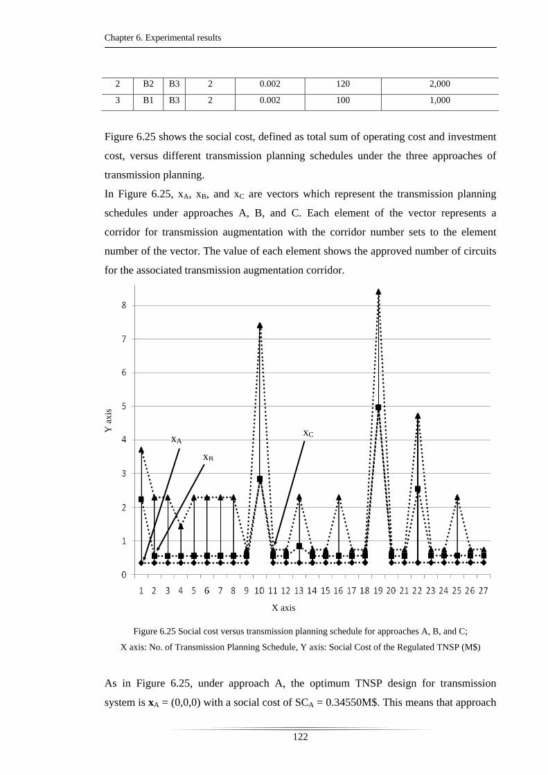
Chapter 6. Experimental results
122
2 B2 B3 2 0.002 120 2,000
3 B1 B3 2 0.002 100 1,000
Figure 6.25 shows the social cost, defined as total sum of operating cost and investment
cost, versus different transmission planning schedules under the three approaches of
transmission planning.
In Figure 6.25, xA, xB, and xC are vectors which represent the transmission planning
schedules under approaches A, B, and C. Each element of the vector represents a
corridor for transmission augmentation with the corridor number sets to the element
number of the vector. The value of each element shows the approved number of circuits
for the associated transmission augmentation corridor.
Figure 6.25 Social cost versus transmission planning schedule for approaches A, B, and C;
X axis: No. of Transmission Planning Schedule, Y axis: Social Cost of the Regulated TNSP (M$)
As in Figure 6.25, under approach A, the optimum TNSP design for transmission
system is xA = (0,0,0) with a social cost of SCA = 0.34550M$. This means that approach
X axis
Y a
xis
xA
xB
xC

Chapter 6. Experimental results
123
A does not approve any circuit for expanding transmission corridors 1, 2, and 3 of Table
6.43. Approach B is employed by the TNSP to model the market power in the process
of transmission expansion planning. xB = (0,0,1) is the transmission planning schedule
with the least social cost, SCB = 0.55822M$, under approach B. xB approves 1 circuit of
transmission line 3 in Table V. Approach C leads to xC = (1,0,1) as the best transmission
planning schedule of the TNSP with SCC = 0.74019M$. This approach approves 1
circuit in each of corridors 1 and 3 of Table 6.43. This approach takes into account the
market power and strategic generation investment in the transmission system design.
The envelope of the social cost curves for approaches A, B, and C are drawn in Figure
6.26, dashed lines. In the 3-node example system, the envelope of the social cost curve
for approach B is located above the envelope for approach A. The reason for this is that
the mathematical structure in (4.23) can model the market power in the process of the
transmission planning. Accordingly, it can calculate the market power cost as a
component of the social cost for the regulated TNSP.
Similarly, the envelope of the social cost curve for approach B is located below that for
approach C. This means that the approach B underestimates the social cost of the
transmission planning schedule as compared with the proposed planning approach C.
This difference comes from the strategic behaviour of the example system’s GenCos in
generation capacity expansion. The mathematical structure in (4.23) models both market
power and strategic generation investment in expansion of the transmission system.
Consequently, the developed mathematical structure can calculate the market power
cost and generation investment cost as the components of the societal cost.
Figure 6.26 shows the underestimation magnitude of the social cost calculated by
approach A and B compared to approach C.
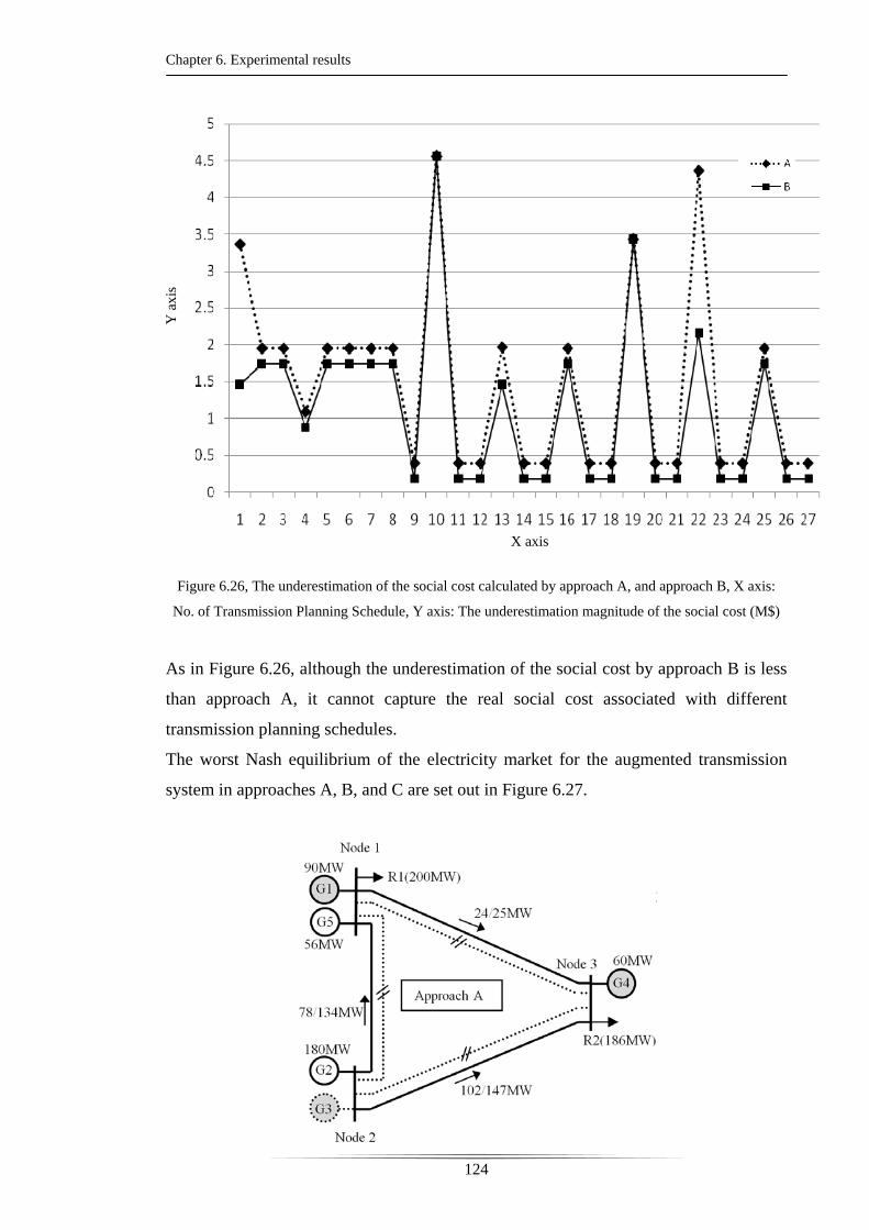
Chapter 6. Experimental results
124
Figure 6.26, The underestimation of the social cost calculated by approach A, and approach B, X axis:
No. of Transmission Planning Schedule, Y axis: The underestimation magnitude of the social cost (M$)
As in Figure 6.26, although the underestimation of the social cost by approach B is less
than approach A, it cannot capture the real social cost associated with different
transmission planning schedules.
The worst Nash equilibrium of the electricity market for the augmented transmission
system in approaches A, B, and C are set out in Figure 6.27.
X axis
Y a
xis

Chapter 6. Experimental results
125
Figure 6.27 Worst Nash equilibrium for the augmented transmission system by approach A, approach B,
and approach C
GenCos 1 and 2 behave strategically to maximise their profit. The price and quantity
bidding of GenCo 1 and GenCo 2 are illustrated in Figure 6.28 through Figure 6.30.
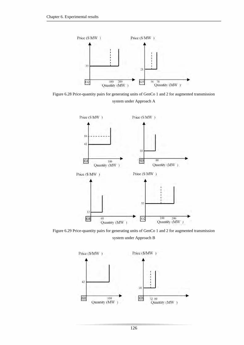
Chapter 6. Experimental results
126
Figure 6.28 Price-quantity pairs for generating units of GenCo 1 and 2 for augmented transmission
system under Approach A
Figure 6.29 Price-quantity pairs for generating units of GenCo 1 and 2 for augmented transmission
system under Approach B
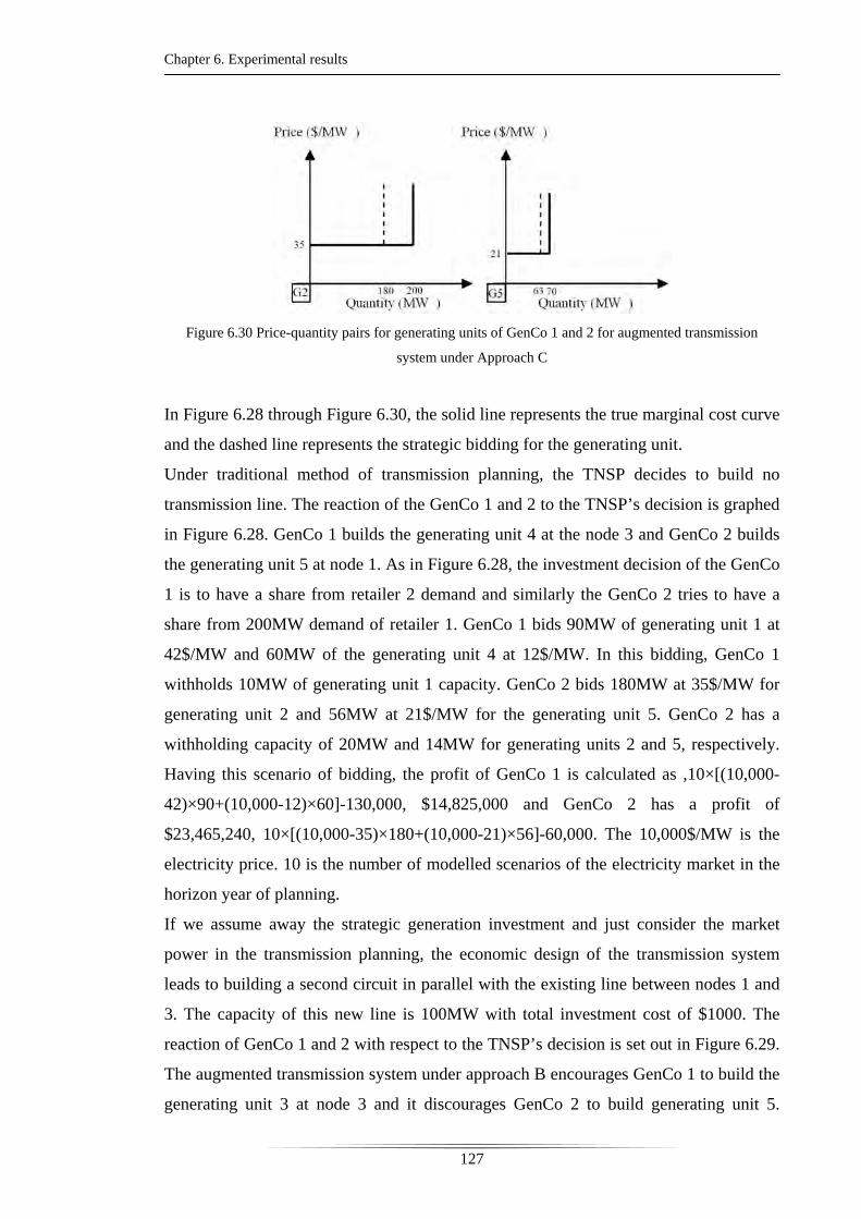
Chapter 6. Experimental results
127
Figure 6.30 Price-quantity pairs for generating units of GenCo 1 and 2 for augmented transmission
system under Approach C
In Figure 6.28 through Figure 6.30, the solid line represents the true marginal cost curve
and the dashed line represents the strategic bidding for the generating unit.
Under traditional method of transmission planning, the TNSP decides to build no
transmission line. The reaction of the GenCo 1 and 2 to the TNSP’s decision is graphed
in Figure 6.28. GenCo 1 builds the generating unit 4 at the node 3 and GenCo 2 builds
the generating unit 5 at node 1. As in Figure 6.28, the investment decision of the GenCo
1 is to have a share from retailer 2 demand and similarly the GenCo 2 tries to have a
share from 200MW demand of retailer 1. GenCo 1 bids 90MW of generating unit 1 at
42$/MW and 60MW of the generating unit 4 at 12$/MW. In this bidding, GenCo 1
withholds 10MW of generating unit 1 capacity. GenCo 2 bids 180MW at 35$/MW for
generating unit 2 and 56MW at 21$/MW for the generating unit 5. GenCo 2 has a
withholding capacity of 20MW and 14MW for generating units 2 and 5, respectively.
Having this scenario of bidding, the profit of GenCo 1 is calculated as ,10×[(10,000-
42)×90+(10,000-12)×60]-130,000, $14,825,000 and GenCo 2 has a profit of
$23,465,240, 10×[(10,000-35)×180+(10,000-21)×56]-60,000. The 10,000$/MW is the
electricity price. 10 is the number of modelled scenarios of the electricity market in the
horizon year of planning.
If we assume away the strategic generation investment and just consider the market
power in the transmission planning, the economic design of the transmission system
leads to building a second circuit in parallel with the existing line between nodes 1 and
3. The capacity of this new line is 100MW with total investment cost of $1000. The
reaction of GenCo 1 and 2 with respect to the TNSP’s decision is set out in Figure 6.29.
The augmented transmission system under approach B encourages GenCo 1 to build the
generating unit 3 at node 3 and it discourages GenCo 2 to build generating unit 5.
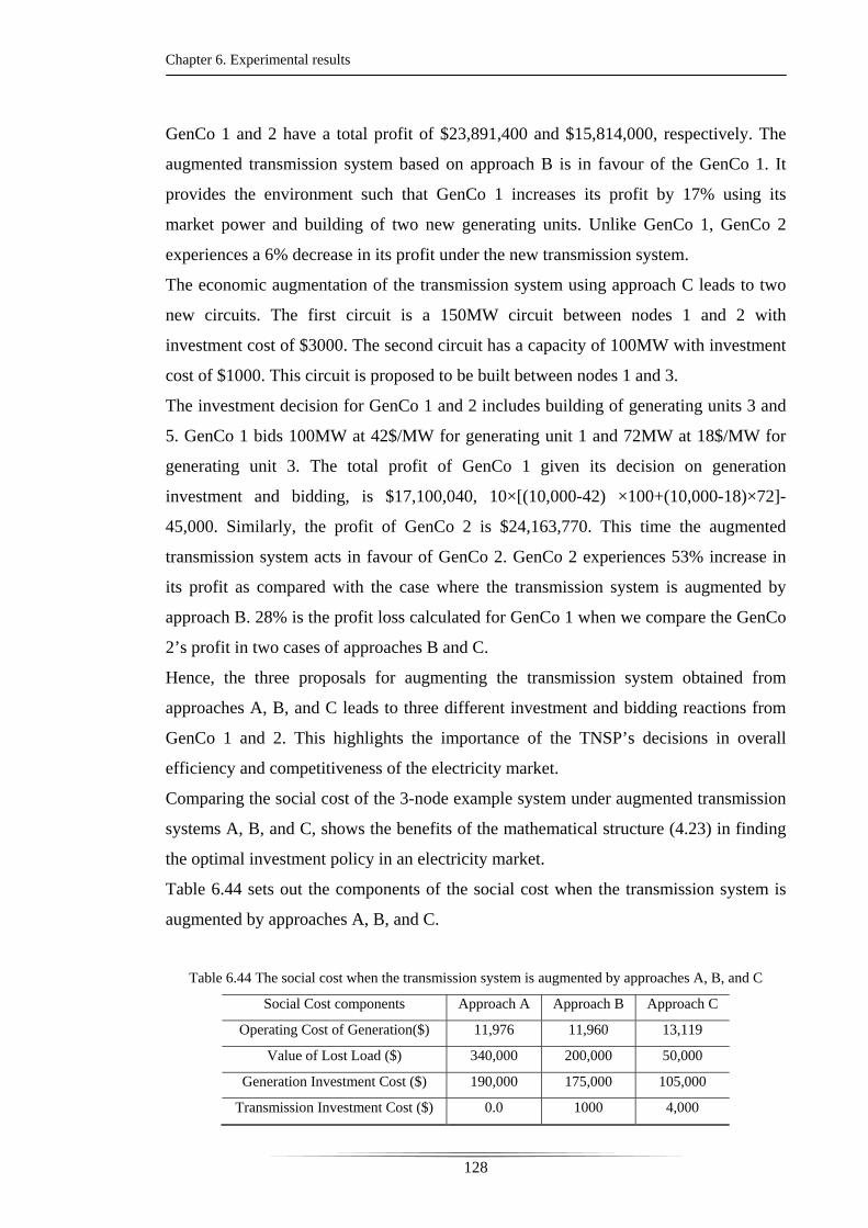
Chapter 6. Experimental results
128
GenCo 1 and 2 have a total profit of $23,891,400 and $15,814,000, respectively. The
augmented transmission system based on approach B is in favour of the GenCo 1. It
provides the environment such that GenCo 1 increases its profit by 17% using its
market power and building of two new generating units. Unlike GenCo 1, GenCo 2
experiences a 6% decrease in its profit under the new transmission system.
The economic augmentation of the transmission system using approach C leads to two
new circuits. The first circuit is a 150MW circuit between nodes 1 and 2 with
investment cost of $3000. The second circuit has a capacity of 100MW with investment
cost of $1000. This circuit is proposed to be built between nodes 1 and 3.
The investment decision for GenCo 1 and 2 includes building of generating units 3 and
5. GenCo 1 bids 100MW at 42$/MW for generating unit 1 and 72MW at 18$/MW for
generating unit 3. The total profit of GenCo 1 given its decision on generation
investment and bidding, is $17,100,040, 10×[(10,000-42) ×100+(10,000-18)×72]-
45,000. Similarly, the profit of GenCo 2 is $24,163,770. This time the augmented
transmission system acts in favour of GenCo 2. GenCo 2 experiences 53% increase in
its profit as compared with the case where the transmission system is augmented by
approach B. 28% is the profit loss calculated for GenCo 1 when we compare the GenCo
2’s profit in two cases of approaches B and C.
Hence, the three proposals for augmenting the transmission system obtained from
approaches A, B, and C leads to three different investment and bidding reactions from
GenCo 1 and 2. This highlights the importance of the TNSP’s decisions in overall
efficiency and competitiveness of the electricity market.
Comparing the social cost of the 3-node example system under augmented transmission
systems A, B, and C, shows the benefits of the mathematical structure (4.23) in finding
the optimal investment policy in an electricity market.
Table 6.44 sets out the components of the social cost when the transmission system is
augmented by approaches A, B, and C.
Table 6.44 The social cost when the transmission system is augmented by approaches A, B, and C
Social Cost components Approach A Approach B Approach C
Operating Cost of Generation($) 11,976 11,960 13,119
Value of Lost Load ($) 340,000 200,000 50,000
Generation Investment Cost ($) 190,000 175,000 105,000
Transmission Investment Cost ($) 0.0 1000 4,000
Chapter 6. Experimental results
129
Social Cost ($) (σ=10.0) 3,709,760 2,295,600 740,190
There is a considerable difference between system social cost under approach C and the
one under approaches A and B as reported in Table 6.44. The optimal investment policy
based on mathematical structure in (4.23), approach C, has a social cost of $740,190 for
the electricity market. The optimal investment policies under approaches B and C have
a social cost of $2,295,600 and $3,709,760, respectively. This is equivalent to 210% and
401% increase in social cost as compared with approach C. This considerable difference
comes from the capability of approach C in modelling of both market power and
strategic generation expansion through its developed mathematical structure in (4.23).
Approach B can only model market power but it can not model the strategic generation
investment of GenCo 1 and 2. The traditional method of economic augmentation of the
transmission system can not model both market power and strategic generation
investment.
The transmission corridor between nodes 1 and 3 was upgraded to 125MW under
approach B. But, in the real situation of the electricity market obtained through the
worst Nash solution, only 16MW flows though this corridor. This is equivalent to a
transmission capacity usage, defined as ratio of transmission line flow and the
transmission line capacity, of 12.8%. This shows the misjudgement of the approach B
on the real value of the transmission capacity. The transmission capacity usages for the
upgraded transmission corridors under approach C is 78.6% and 47.6%.
In Figure 6.31 and Figure 6.32, we quantify the total benefit of the transmission
planning schedules, xA=(0,0,0), xB=(0,0,1), and xC=(1,0,1) into the efficiency benefit,
competition benefit, and saving in transmission investment cost. The quantifying
scheme in section 4.6 highlights the benefits of the proposed structure in (4.23) as
compared to the (4.18) and (4.24).
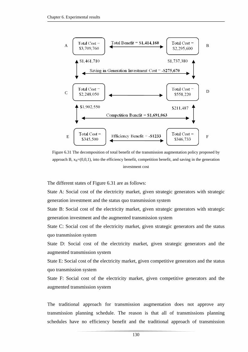
Chapter 6. Experimental results
130
Figure 6.31 The decomposition of total benefit of the transmission augmentation policy proposed by
approach B, xB=(0,0,1), into the efficiency benefit, competition benefit, and saving in the generation
investment cost
The different states of Figure 6.31 are as follows:
State A: Social cost of the electricity market, given strategic generators with strategic
generation investment and the status quo transmission system
State B: Social cost of the electricity market, given strategic generators with strategic
generation investment and the augmented transmission system
State C: Social cost of the electricity market, given strategic generators and the status
quo transmission system
State D: Social cost of the electricity market, given strategic generators and the
augmented transmission system
State E: Social cost of the electricity market, given competitive generators and the status
quo transmission system
State F: Social cost of the electricity market, given competitive generators and the
augmented transmission system
The traditional approach for transmission augmentation does not approve any
transmission planning schedule. The reason is that all of transmissions planning
schedules have no efficiency benefit and the traditional approach of transmission
A B
C D
E F
Chapter 6. Experimental results
131
augmentation can only capture the efficiency benefit. Approach B proposes xB=(0,0,1)
as the transmission planning schedule. As in Figure 6.31, the proposed planning
schedule has negative efficiency benefit, and negative saving in generation investment
cost. But, the competition benefit of the proposed planning schedule is big enough to
justify the transmission augmentation schedule.
The transmission planning schedule proposed by approach C, has a higher total benefit
as compared to the one proposed by approach B, 52%. Comparing the elements of the
total benefit reveals that the main difference is in the saving in generation cost. This
element of total benefit can be captured by the mathematical structure derived in (4.23).
Figure 6.31 and Figure 6.32 highlight the strong points of the derived structure in this
paper for evaluating the transmission augmentation policies. Approach A only captures
the efficiency benefit of a transmission augmentation policy. It ignores the competition
benefit and the effect of additional transmission capacity on generation investment
decisions. Approach B models the efficiency benefit and the competition benefit of a
transmission augmentation policy and it can not model the impact of additional
transmission capacity on generation investment decisions. Accordingly, both
approaches A, and B can not judge the transmission augmentation policies based on
their real value. The proposed approach by this paper, approach C, models the three
main benefits of transmission augmentation policies in a mathematical structure and it
can capture the main benefits of transmission augmentation policies in its decision
making process.
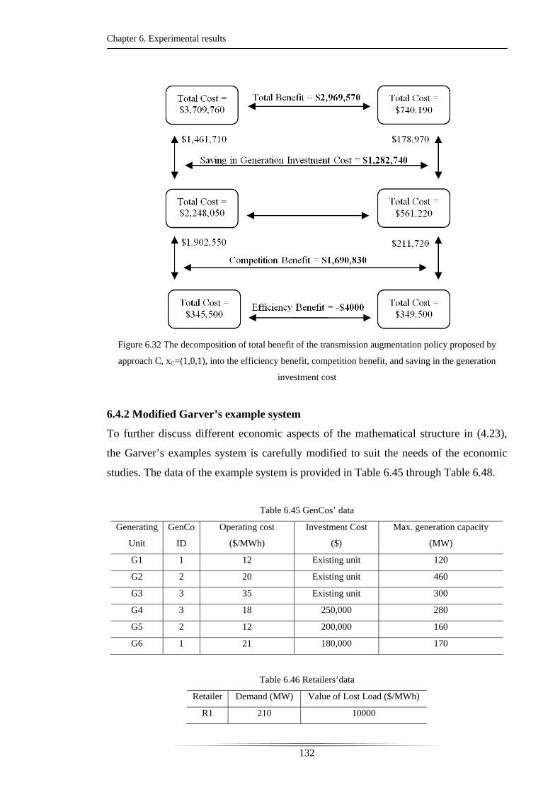
Chapter 6. Experimental results
132
Figure 6.32 The decomposition of total benefit of the transmission augmentation policy proposed by
approach C, xC=(1,0,1), into the efficiency benefit, competition benefit, and saving in the generation
investment cost
6.4.2 Modified Garver’s example system
To further discuss different economic aspects of the mathematical structure in (4.23),
the Garver’s examples system is carefully modified to suit the needs of the economic
studies. The data of the example system is provided in Table 6.45 through Table 6.48.
Table 6.45 GenCos’ data
Generating
Unit
GenCo
ID
Operating cost
($/MWh)
Investment Cost
($)
Max. generation capacity
(MW)
G1 1 12 Existing unit 120
G2 2 20 Existing unit 460
G3 3 35 Existing unit 300
G4 3 18 250,000 280
G5 2 12 200,000 160
G6 1 21 180,000 170
Table 6.46 Retailers’data
Retailer Demand (MW) Value of Lost Load ($/MWh)
R1 210 10000
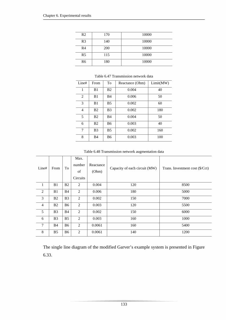
Chapter 6. Experimental results
133
R2 170 10000
R3 140 10000
R4 200 10000
R5 115 10000
R6 180 10000
Table 6.47 Transmission network data
Line# From To Reactance (Ohm) Limit(MW)
1 B1 B2 0.004 40
2 B1 B4 0.006 50
3 B1 B5 0.002 60
4 B2 B3 0.002 180
5 B2 B4 0.004 50
6 B2 B6 0.003 40
7 B3 B5 0.002 160
8 B4 B6 0.003 100
Table 6.48 Transmission network augmentation data
Line# From To
Max.
number
of
Circuits
Reactance
(Ohm) Capacity of each circuit (MW) Trans. Investment cost ($/Cct)
1 B1 B2 2 0.004 120 8500
2 B1 B4 2 0.006 180 5000
3 B2 B3 2 0.002 150 7000
4 B2 B6 2 0.003 120 5500
5 B3 B4 2 0.002 150 6000
6 B3 B5 2 0.003 160 1000
7 B4 B6 2 0.0061 160 5400
8 B5 B6 2 0.0061 140 1200
The single line diagram of the modified Garver’s example system is presented in Figure
6.33.
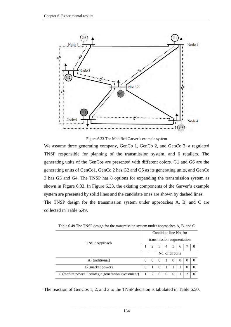
Chapter 6. Experimental results
134
Figure 6.33 The Modified Garver’s example system
We assume three generating company, GenCo 1, GenCo 2, and GenCo 3, a regulated
TNSP responsible for planning of the transmission system, and 6 retailers. The
generating units of the GenCos are presented with different colors. G1 and G6 are the
generating units of GenCo1. GenCo 2 has G2 and G5 as its generating units, and GenCo
3 has G3 and G4. The TNSP has 8 options for expanding the transmission system as
shown in Figure 6.33. In Figure 6.33, the existing components of the Garver’s example
system are presented by solid lines and the candidate ones are shown by dashed lines.
The TNSP design for the transmission system under approaches A, B, and C are
collected in Table 6.49.
Table 6.49 The TNSP design for the transmission system under approaches A, B, and C
TNSP Approach
Candidate line No. for
transmission augmentation
1 2 3 4 5 6 7 8
No. of circuits
A (traditional) 0 0 0 1 0 0 0 0
B (market power) 0 1 0 1 1 1 0 0
C (market power + strategic generation investment) 1 2 0 0 0 1 2 0
The reaction of GenCos 1, 2, and 3 to the TNSP decision is tabulated in Table 6.50.
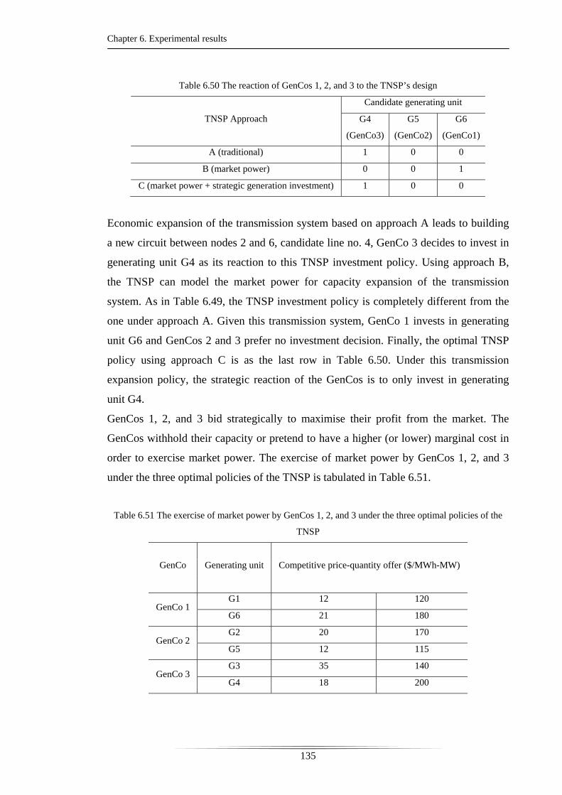
Chapter 6. Experimental results
135
Table 6.50 The reaction of GenCos 1, 2, and 3 to the TNSP’s design
TNSP Approach
Candidate generating unit
G4
(GenCo3)
G5
(GenCo2)
G6
(GenCo1)
A (traditional) 1 0 0
B (market power) 0 0 1
C (market power + strategic generation investment) 1 0 0
Economic expansion of the transmission system based on approach A leads to building
a new circuit between nodes 2 and 6, candidate line no. 4, GenCo 3 decides to invest in
generating unit G4 as its reaction to this TNSP investment policy. Using approach B,
the TNSP can model the market power for capacity expansion of the transmission
system. As in Table 6.49, the TNSP investment policy is completely different from the
one under approach A. Given this transmission system, GenCo 1 invests in generating
unit G6 and GenCos 2 and 3 prefer no investment decision. Finally, the optimal TNSP
policy using approach C is as the last row in Table 6.50. Under this transmission
expansion policy, the strategic reaction of the GenCos is to only invest in generating
unit G4.
GenCos 1, 2, and 3 bid strategically to maximise their profit from the market. The
GenCos withhold their capacity or pretend to have a higher (or lower) marginal cost in
order to exercise market power. The exercise of market power by GenCos 1, 2, and 3
under the three optimal policies of the TNSP is tabulated in Table 6.51.
Table 6.51 The exercise of market power by GenCos 1, 2, and 3 under the three optimal policies of the
TNSP
GenCo Generating unit Competitive price-quantity offer ($/MWh-MW)
GenCo 1 G1 12 120
G6 21 180
GenCo 2 G2 20 170
G5 12 115
GenCo 3 G3 35 140
G4 18 200
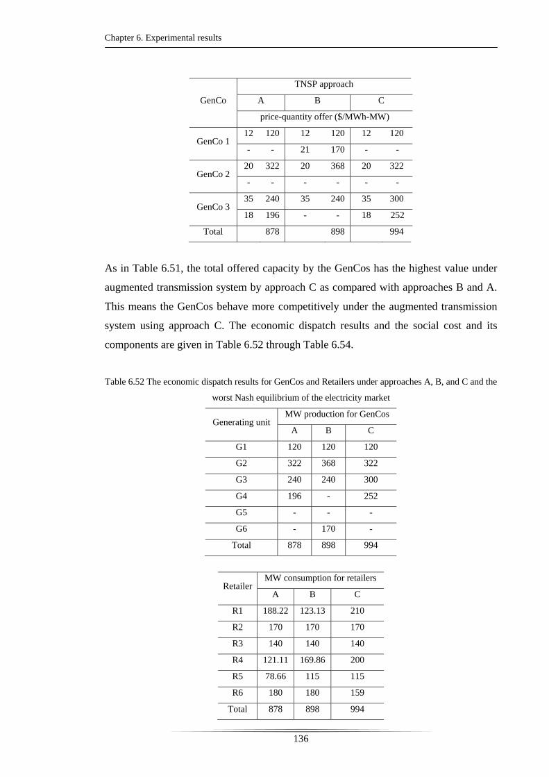
Chapter 6. Experimental results
136
GenCo
TNSP approach
A B C
price-quantity offer ($/MWh-MW)
GenCo 1 12 120 12 120 12 120
- - 21 170 - -
GenCo 2 20 322 20 368 20 322
- - - - - -
GenCo 3 35 240 35 240 35 300
18 196 - - 18 252
Total 878 898 994
As in Table 6.51, the total offered capacity by the GenCos has the highest value under
augmented transmission system by approach C as compared with approaches B and A.
This means the GenCos behave more competitively under the augmented transmission
system using approach C. The economic dispatch results and the social cost and its
components are given in Table 6.52 through Table 6.54.
Table 6.52 The economic dispatch results for GenCos and Retailers under approaches A, B, and C and the
worst Nash equilibrium of the electricity market
Generating unit MW production for GenCos
A B C
G1 120 120 120
G2 322 368 322
G3 240 240 300
G4 196 - 252
G5 - - -
G6 - 170 -
Total 878 898 994
Retailer MW consumption for retailers
A B C
R1 188.22 123.13 210
R2 170 170 170
R3 140 140 140
R4 121.11 169.86 200
R5 78.66 115 115
R6 180 180 159
Total 878 898 994
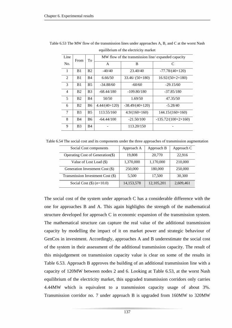
Chapter 6. Experimental results
137
Table 6.53 The MW flow of the transmission lines under approaches A, B, and C at the worst Nash
equilibrium of the electricity market
Line
No. From To
MW flow of the transmission line/ expanded capacity
A B C
1 B1 B2 -40/40 23.40/40 -77.78/(40+120)
2 B1 B4 6.66/50 33.46/ (50+180) 16.92/(50+2×180)
3 B1 B5 -34.88/60 -60/60 -29.15/60
4 B2 B3 -68.44/180 -109.80/180 -37.85/180
5 B2 B4 50/50 1.69/50 47.35/50
6 B2 B6 4.44/(40+120) -38.49/(40+120) -5.28/40
7 B3 B5 113.55/160 4.9/(160+160) 144.15/(160+160)
8 B4 B6 -64.44/100 -21.50/100 -135.72/(100+2×160)
9 B3 B4 - 113.20/150 -
Table 6.54 The social cost and its components under the three approaches of transmission augmentation
Social Cost components Approach A Approach B Approach C
Operating Cost of Generation($) 19,808 20,770 22,916
Value of Lost Load ($) 1,370,000 1,170,000 210,000
Generation Investment Cost ($) 250,000 180,000 250,000
Transmission Investment Cost ($) 5,500 17,500 30,300
Social Cost ($) (σ=10.0) 14,153,578 12,105,201 2,609,461
The social cost of the system under approach C has a considerable difference with the
one for approaches B and A. This again highlights the strength of the mathematical
structure developed for approach C in economic expansion of the transmission system.
The mathematical structure can capture the real value of the additional transmission
capacity by modelling the impact of it on market power and strategic behaviour of
GenCos in investment. Accordingly, approaches A and B underestimate the social cost
of the system in their assessment of the additional transmission capacity. The result of
this misjudgement on transmission capacity value is clear on some of the results in
Table 6.53. Approach B approves the building of an additional transmission line with a
capacity of 120MW between nodes 2 and 6. Looking at Table 6.53, at the worst Nash
equilibrium of the electricity market, this upgraded transmission corridors only carries
4.44MW which is equivalent to a transmission capacity usage of about 3%.
Transmission corridor no. 7 under approach B is upgraded from 160MW to 320MW
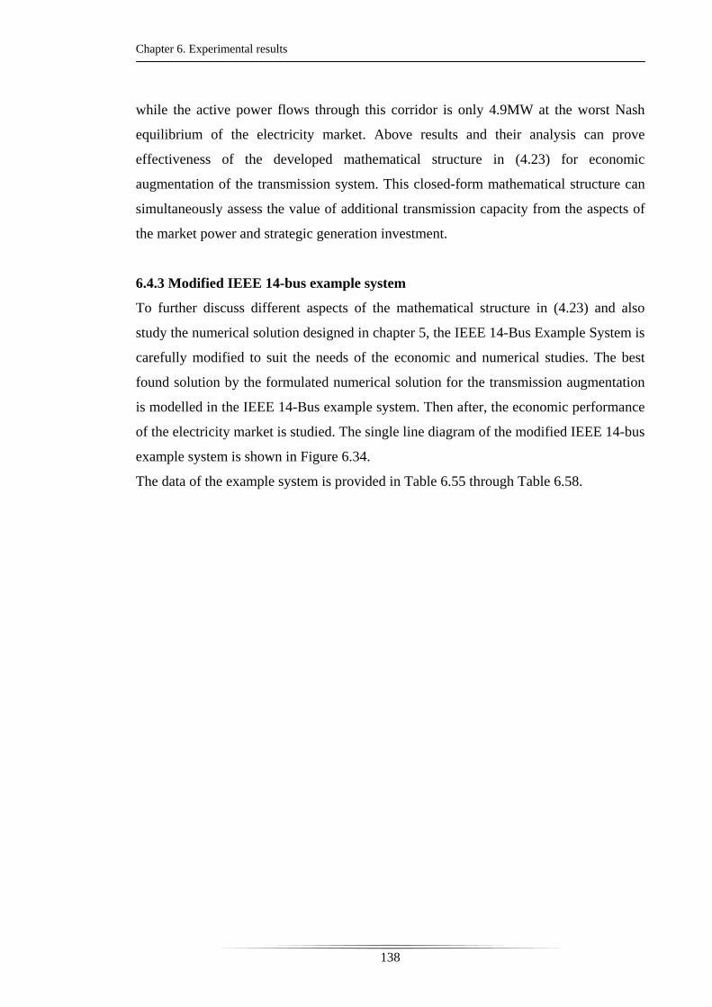
Chapter 6. Experimental results
138
while the active power flows through this corridor is only 4.9MW at the worst Nash
equilibrium of the electricity market. Above results and their analysis can prove
effectiveness of the developed mathematical structure in (4.23) for economic
augmentation of the transmission system. This closed-form mathematical structure can
simultaneously assess the value of additional transmission capacity from the aspects of
the market power and strategic generation investment.
6.4.3 Modified IEEE 14-bus example system
To further discuss different aspects of the mathematical structure in (4.23) and also
study the numerical solution designed in chapter 5, the IEEE 14-Bus Example System is
carefully modified to suit the needs of the economic and numerical studies. The best
found solution by the formulated numerical solution for the transmission augmentation
is modelled in the IEEE 14-Bus example system. Then after, the economic performance
of the electricity market is studied. The single line diagram of the modified IEEE 14-bus
example system is shown in Figure 6.34.
The data of the example system is provided in Table 6.55 through Table 6.58.
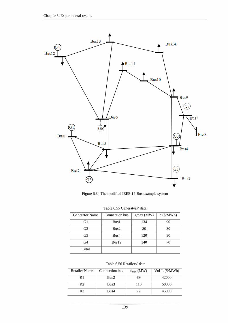
Chapter 6. Experimental results
139
Figure 6.34 The modified IEEE 14-Bus example system
Table 6.55 Generators’ data
Generator Name Connection bus gmax (MW) c ($/MWh)
G1 Bus1 134 90
G2 Bus2 80 30
G3 Bus4 120 50
G4 Bus12 140 70
Total
Table 6.56 Retailers’ data
Retailer Name Connection bus dmax (MW) VoLL ($/MWh)
R1 Bus2 89 42000
R2 Bus3 110 50000
R3 Bus4 72 45000
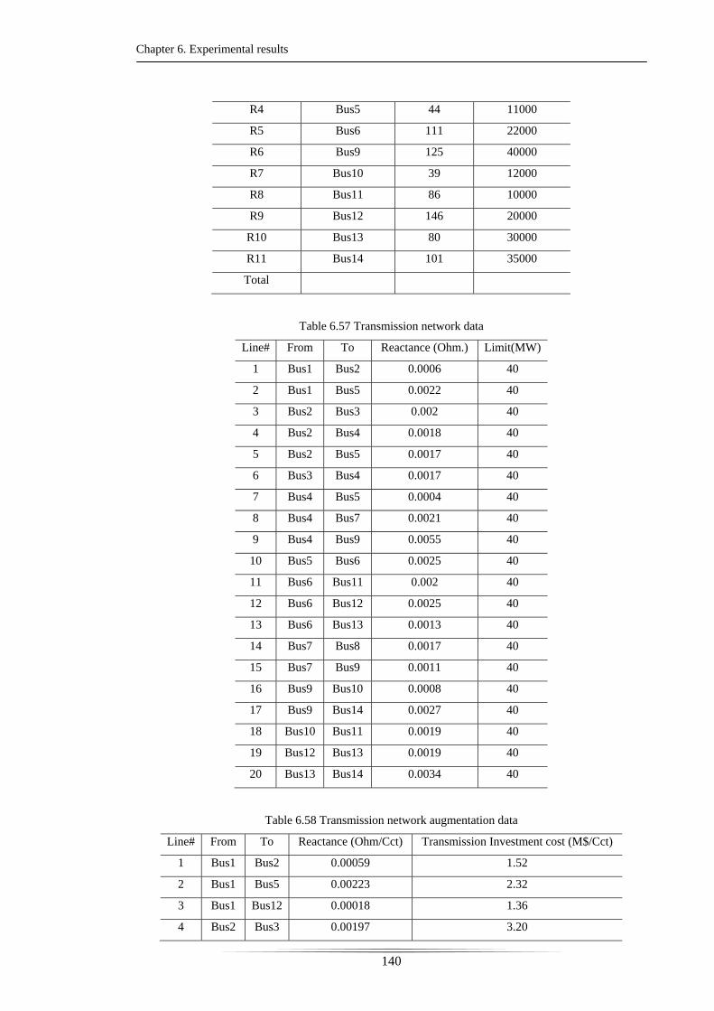
Chapter 6. Experimental results
140
R4 Bus5 44 11000
R5 Bus6 111 22000
R6 Bus9 125 40000
R7 Bus10 39 12000
R8 Bus11 86 10000
R9 Bus12 146 20000
R10 Bus13 80 30000
R11 Bus14 101 35000
Total
Table 6.57 Transmission network data
Line# From To Reactance (Ohm.) Limit(MW)
1 Bus1 Bus2 0.0006 40
2 Bus1 Bus5 0.0022 40
3 Bus2 Bus3 0.002 40
4 Bus2 Bus4 0.0018 40
5 Bus2 Bus5 0.0017 40
6 Bus3 Bus4 0.0017 40
7 Bus4 Bus5 0.0004 40
8 Bus4 Bus7 0.0021 40
9 Bus4 Bus9 0.0055 40
10 Bus5 Bus6 0.0025 40
11 Bus6 Bus11 0.002 40
12 Bus6 Bus12 0.0025 40
13 Bus6 Bus13 0.0013 40
14 Bus7 Bus8 0.0017 40
15 Bus7 Bus9 0.0011 40
16 Bus9 Bus10 0.0008 40
17 Bus9 Bus14 0.0027 40
18 Bus10 Bus11 0.0019 40
19 Bus12 Bus13 0.0019 40
20 Bus13 Bus14 0.0034 40
Table 6.58 Transmission network augmentation data
Line# From To Reactance (Ohm/Cct) Transmission Investment cost (M$/Cct)
1 Bus1 Bus2 0.00059 1.52
2 Bus1 Bus5 0.00223 2.32
3 Bus1 Bus12 0.00018 1.36
4 Bus2 Bus3 0.00197 3.20
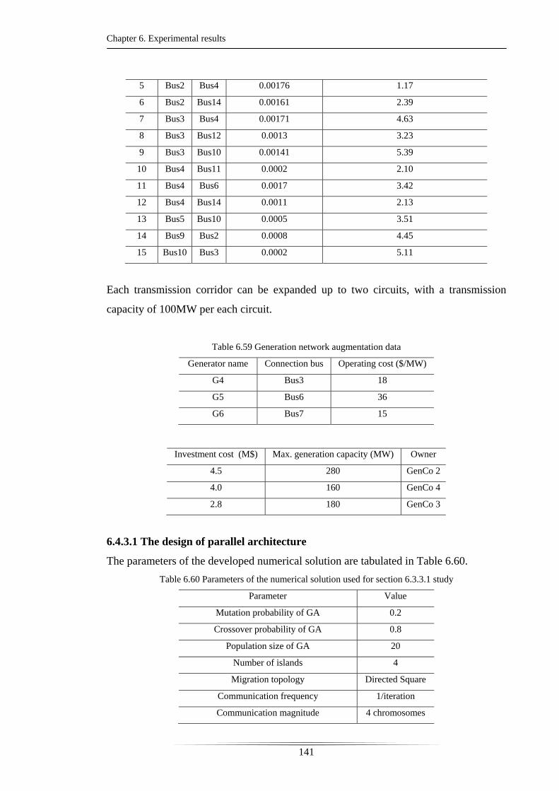
Chapter 6. Experimental results
141
5 Bus2 Bus4 0.00176 1.17
6 Bus2 Bus14 0.00161 2.39
7 Bus3 Bus4 0.00171 4.63
8 Bus3 Bus12 0.0013 3.23
9 Bus3 Bus10 0.00141 5.39
10 Bus4 Bus11 0.0002 2.10
11 Bus4 Bus6 0.0017 3.42
12 Bus4 Bus14 0.0011 2.13
13 Bus5 Bus10 0.0005 3.51
14 Bus9 Bus2 0.0008 4.45
15 Bus10 Bus3 0.0002 5.11
Each transmission corridor can be expanded up to two circuits, with a transmission
capacity of 100MW per each circuit.
Table 6.59 Generation network augmentation data
Generator name Connection bus Operating cost ($/MW)
G4 Bus3 18
G5 Bus6 36
G6 Bus7 15
Investment cost (M$) Max. generation capacity (MW) Owner
4.5 280 GenCo 2
4.0 160 GenCo 4
2.8 180 GenCo 3
6.4.3.1 The design of parallel architecture
The parameters of the developed numerical solution are tabulated in Table 6.60.
Table 6.60 Parameters of the numerical solution used for section 6.3.3.1 study
Parameter Value
Mutation probability of GA 0.2
Crossover probability of GA 0.8
Population size of GA 20
Number of islands 4
Migration topology Directed Square
Communication frequency 1/iteration
Communication magnitude 4 chromosomes
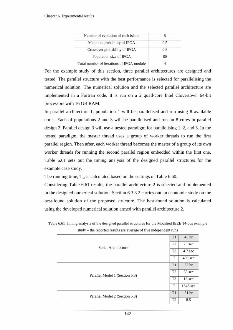
Chapter 6. Experimental results
142
Number of evolution of each island 5
Mutation probability of IPGA 0.5
Crossover probability of IPGA 0.8
Population size of IPGA 80
Total number of iterations of IPGA module 4
For the example study of this section, three parallel architectures are designed and
tested. The parallel structure with the best performance is selected for parallelising the
numerical solution. The numerical solution and the selected parallel architecture are
implemented in a Fortran code. It is run on a 2 quad-core Intel Clovertown 64-bit
processors with 16 GB RAM.
In parallel architecture 1, population 1 will be parallelised and run using 8 available
cores. Each of populations 2 and 3 will be parallelised and run on 8 cores in parallel
design 2. Parallel design 3 will use a nested paradigm for parallelising 1, 2, and 3. In the
nested paradigm, the master thread uses a group of worker threads to run the first
parallel region. Then after, each worker thread becomes the master of a group of its own
worker threads for running the second parallel region embedded within the first one.
Table 6.61 sets out the timing analysis of the designed parallel structures for the
example case study.
The running time, T1, is calculated based on the settings of Table 6.60.
Considering Table 6.61 results, the parallel architecture 2 is selected and implemented
in the designed numerical solution. Section 6.3.3.2 carries out an economic study on the
best-found solution of the proposed structure. The best-found solution is calculated
using the developed numerical solution armed with parallel architecture 2.
Table 6.61 Timing analysis of the designed parallel structures for the Modified IEEE 14-bus example
study – the reported results are average of five independent runs
Serial Architecture
T1 45 hr
T2 23 sec
T3 4.7 sec
T 400 sec
Parallel Model 1 (Section 5.3)
T1 23 hr
T2 63 sec
T3 16 sec
T 1343 sec
Parallel Model 2 (Section 5.3) T1 21 hr
T2 8.5
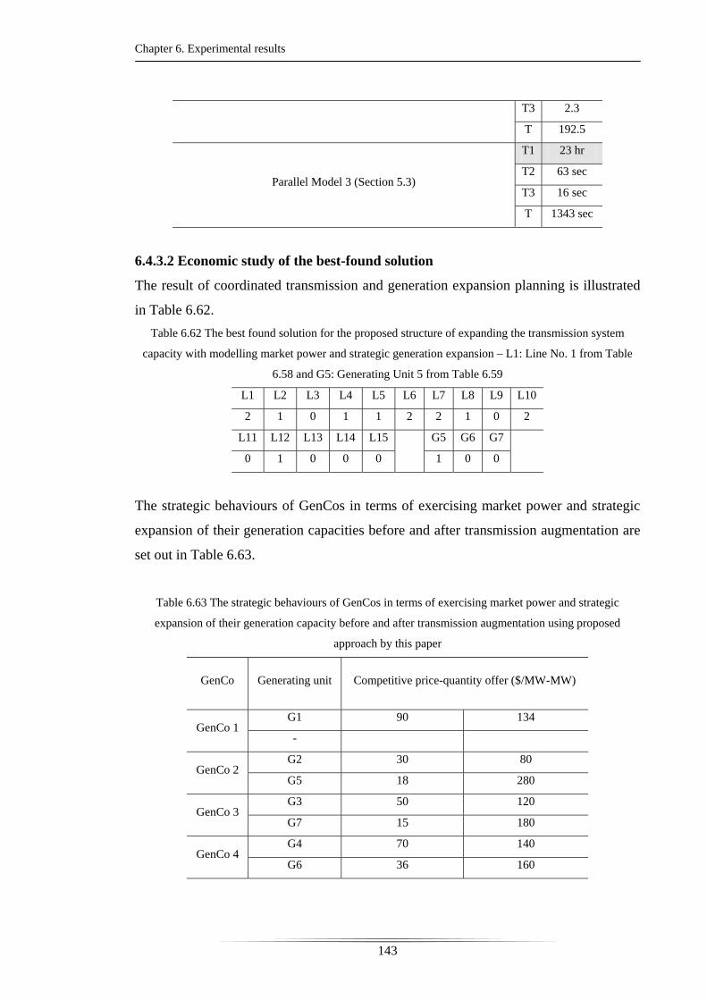
Chapter 6. Experimental results
143
T3 2.3
T 192.5
Parallel Model 3 (Section 5.3)
T1 23 hr
T2 63 sec
T3 16 sec
T 1343 sec
6.4.3.2 Economic study of the best-found solution
The result of coordinated transmission and generation expansion planning is illustrated
in Table 6.62.
Table 6.62 The best found solution for the proposed structure of expanding the transmission system
capacity with modelling market power and strategic generation expansion – L1: Line No. 1 from Table
6.58 and G5: Generating Unit 5 from Table 6.59
L1 L2 L3 L4 L5 L6 L7 L8 L9 L10
2 1 0 1 1 2 2 1 0 2
L11 L12 L13 L14 L15
G5 G6 G7
0 1 0 0 0 1 0 0
The strategic behaviours of GenCos in terms of exercising market power and strategic
expansion of their generation capacities before and after transmission augmentation are
set out in Table 6.63.
Table 6.63 The strategic behaviours of GenCos in terms of exercising market power and strategic
expansion of their generation capacity before and after transmission augmentation using proposed
approach by this paper
GenCo Generating unit Competitive price-quantity offer ($/MW-MW)
GenCo 1 G1 90 134
-
GenCo 2 G2 30 80
G5 18 280
GenCo 3 G3 50 120
G7 15 180
GenCo 4 G4 70 140
G6 36 160

Chapter 6. Experimental results
144
GenCo Status quo transmission system Augmented transmission system using proposed approach
Actual price-quantity offer ($/MW-MW)
GenCo 1 90 80.4 90 134
- -
GenCo 2 30 80 30 80
No Investment 18 280
GenCo 3 50 120 50 120
No Investment No Investment
GenCo 4 70 140 70 140
No Investment No Investment
Total 420.4MW 754MW (79%INC)
INC: Increase
In the status quo transmission system, GenCo 1 withholds 53.6MW of generating unit 1
and offer only 80.4MW to the EMO. GenCos 2, 3, and 4 decide not to invest in new
generating units of G5, G6, and G7. In this case the total offered capacity by the
generation sector to the EMO is 420.4MW. Given this state of the electricity market, the
TNSP designs the transmission system as set out in Table 6.62. The TNSP investment
decision is based on mathematical structure in (4.23). Accordingly, it considers the
market power effect and the strategic generation capacity expansion. The TNSP
decision has two effects, first: market power effect, the offered capacity of G1 is
increased from 80.4MW to 134MW, and second: strategic generation capacity
expansion, GenCo 2 decides to invest in G5. This investment decision in generation
capacity will increase the total offered capacity from 420.4MW to 754MW which is
equivalent to 79% increase.
In Table 6.64 through Table 6.67 results of the security-constrained economic dispatch
are tabulated.
Table 6.64 The economic dispatch results for GenCos and Retailers at the best-found worst Nash
equilibrium of the electricity market in the status quo transmission system
Bus No. Voltage Angle (Radian) Generation (MW) Load (MW) LP* ($/MWh)
1 0.0000 55.5 0.0 90
2 -0.0240 80 61.11 42000
3 -0.1040 - 73.34 50000
4 -0.0473 120 72 37326
5 -0.0341 - 0.0 33370

Chapter 6. Experimental results
145
6 -0.0051 - 0.0 33767
7 -0.1278 - 0.0 37115
8 -0.1278 - 0.0 37115
9 -0.1700 - 125 37005
10 -0.1419 - 0.0 36454
11 -0.0753 - 0.0 35145
12 0.0848 140 64 20000
13 0.0088 - 0.0 40237
14 -0.0908 - 0.0 38436
Total/Installed 395.5/420.4 395.5/395.5
Average of Nodal Prices($/MWh) 34,147
LP* : Locational Price
Table 6.65 The MW flow of the transmission lines at the best-found worst Nash equilibrium - the status
quo transmission system
Branch
No. From To Power Flow (MW)
1 Bus1 Bus2 40.00 (Congested)
2 Bus1 Bus5 15.5
3 Bus2 Bus3 40.00 (Congested)
4 Bus2 Bus4 12.95
5 Bus2 Bus5 5.94
6 Bus3 Bus4 -33.35
7 Bus4 Bus5 -33.03
8 Bus4 Bus7 38.33
9 Bus4 Bus9 22.30
10 Bus5 Bus6 -11.59
11 Bus6 Bus11 35.07
12 Bus6 Bus12 -35.96
13 Bus6 Bus13 -10.70
14 Bus7 Bus8 0.00
15 Bus7 Bus9 38.33
16 Bus9 Bus10 -35.07
17 Bus9 Bus14 -29.30
18 Bus10 Bus11 -35.07
19 Bus12 Bus13 40.00 (Congested)
20 Bus13 Bus14 29.30
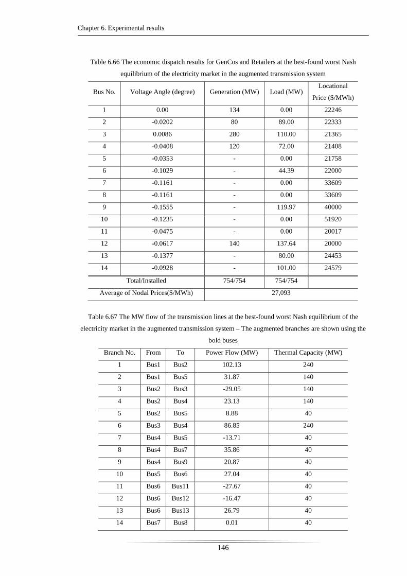
Chapter 6. Experimental results
146
Table 6.66 The economic dispatch results for GenCos and Retailers at the best-found worst Nash
equilibrium of the electricity market in the augmented transmission system
Bus No. Voltage Angle (degree) Generation (MW) Load (MW) Locational
Price ($/MWh)
1 0.00 134 0.00 22246
2 -0.0202 80 89.00 22333
3 0.0086 280 110.00 21365
4 -0.0408 120 72.00 21408
5 -0.0353 - 0.00 21758
6 -0.1029 - 44.39 22000
7 -0.1161 - 0.00 33609
8 -0.1161 - 0.00 33609
9 -0.1555 - 119.97 40000
10 -0.1235 - 0.00 51920
11 -0.0475 - 0.00 20017
12 -0.0617 140 137.64 20000
13 -0.1377 - 80.00 24453
14 -0.0928 - 101.00 24579
Total/Installed 754/754 754/754
Average of Nodal Prices($/MWh) 27,093
Table 6.67 The MW flow of the transmission lines at the best-found worst Nash equilibrium of the
electricity market in the augmented transmission system – The augmented branches are shown using the
bold buses
Branch No. From To Power Flow (MW) Thermal Capacity (MW)
1 Bus1 Bus2 102.13 240
2 Bus1 Bus5 31.87 140
3 Bus2 Bus3 -29.05 140
4 Bus2 Bus4 23.13 140
5 Bus2 Bus5 8.88 40
6 Bus3 Bus4 86.85 240
7 Bus4 Bus5 -13.71 40
8 Bus4 Bus7 35.86 40
9 Bus4 Bus9 20.87 40
10 Bus5 Bus6 27.04 40
11 Bus6 Bus11 -27.67 40
12 Bus6 Bus12 -16.47 40
13 Bus6 Bus13 26.79 40
14 Bus7 Bus8 0.01 40
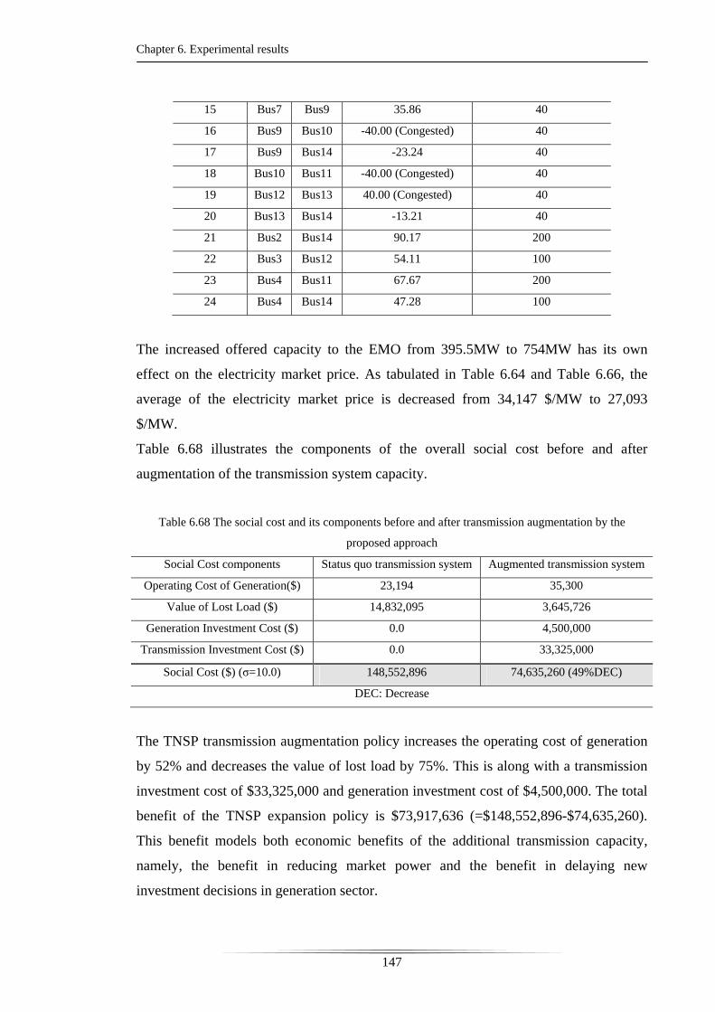
Chapter 6. Experimental results
147
15 Bus7 Bus9 35.86 40
16 Bus9 Bus10 -40.00 (Congested) 40
17 Bus9 Bus14 -23.24 40
18 Bus10 Bus11 -40.00 (Congested) 40
19 Bus12 Bus13 40.00 (Congested) 40
20 Bus13 Bus14 -13.21 40
21 Bus2 Bus14 90.17 200
22 Bus3 Bus12 54.11 100
23 Bus4 Bus11 67.67 200
24 Bus4 Bus14 47.28 100
The increased offered capacity to the EMO from 395.5MW to 754MW has its own
effect on the electricity market price. As tabulated in Table 6.64 and Table 6.66, the
average of the electricity market price is decreased from 34,147 $/MW to 27,093
$/MW.
Table 6.68 illustrates the components of the overall social cost before and after
augmentation of the transmission system capacity.
Table 6.68 The social cost and its components before and after transmission augmentation by the
proposed approach
Social Cost components Status quo transmission system Augmented transmission system
Operating Cost of Generation($) 23,194 35,300
Value of Lost Load ($) 14,832,095 3,645,726
Generation Investment Cost ($) 0.0 4,500,000
Transmission Investment Cost ($) 0.0 33,325,000
Social Cost ($) (σ=10.0) 148,552,896 74,635,260 (49%DEC)
DEC: Decrease
The TNSP transmission augmentation policy increases the operating cost of generation
by 52% and decreases the value of lost load by 75%. This is along with a transmission
investment cost of $33,325,000 and generation investment cost of $4,500,000. The total
benefit of the TNSP expansion policy is $73,917,636 (=$148,552,896-$74,635,260).
This benefit models both economic benefits of the additional transmission capacity,
namely, the benefit in reducing market power and the benefit in delaying new
investment decisions in generation sector.
Chapter 6. Experimental results
148
6.5 Chapter summary
This chapter deals with the economic assessment of the optimisation approaches
developed in chapter 4 and the solution algorithm developed in chapter 5. Section 6.2
analyses the first and the second approach for assessing transmission augmentation.
Section 6.3 assesses the third approach of transmission augmentation which is
developed for modeling of the efficiency benefit and competition benefit of the
additional transmission capacity. The fourth approach for economically-efficient
transmission augmentation is assessed in section 6.4. In the numerical analysis, two sets
of experiments are carried out. The first set employs the modified three-node example
system and the modified Garver’s example system to explain the economics of the
developed mathematical structures. In the second set, the modified IEEE 14-bus
example system is used. Using this case study, the developed numerical algorithm, HB
GA/IPGA, is tested. High performance computing techniques are employed to improve
the efficiency of the HB GA/IPGA.

CHAPTER 7 – CONCLUDING REMARKS AND FUTURE
WORKS
Chapter 7 Concluding remarks and future works
150
7.1 Concluding remarks
In this research work, I developed four different mathematical structures for augmentation
of the transmission systems in the liberalised electricity markets. The first structure
employs the concepts of the financial withholding and physical withholding in a metric
termed L-Shape area metric. The second approach uses the competitive social cost as a
measure of the efficiency and the monopoly rent as a measure of the competitiveness.
Based on these concepts, the mathematical structure of the TNSP is derived. The economic
concept of the social welfare or social cost is employed for deriving the third and fourth
mathematical structures. The third mathematical structure models the efficiency benefit and
competition benefit of the additional transmission capacity in its process of augmentation.
The fourth mathematical structure models the efficiency benefit, the competition benefit
and the strategic expansion of the generation sector. A quantifying approach is designed to
decompose the total benefit of additional transmission capacity into the efficiency benefit,
the competition benefit, and saving in generation investment cost.
Between the first three approaches, approach 3 is proposed by this research work. It (1) is
consistent with current framework of the Australian National Electricity Market, (2) has a
sound economic meaning, (3) has a single function in the TNSP objective function,
mathematically it is a single objective optimisation problem, (4) can employ the
decomposition technique introduced by the Australian Energy Regulator.
Approach 4 is the extension of the approach 3 for modelling the strategic generation
investment decisions.
A numerical solution termed Hybrid Bilevel Genetic Algorithm/Island Parallel Genetic
Algorithm, HB GA/IPGA, to solve the derived mathematical structures. The HB GA/IPGA
has two levels. The GA deals with the TNSP’s decision variables and the IPGA deals with
the bidding behaviors of the rival GenCos participating in the electricity market. The IPGA
module uses the concept of parallel islands in finding the set of Nash equilibriums of the
electricity market. In doing so, each island explores the set of possible biddings of the
GenCos independently for finding the Nash equilibriums. To improve the efficiency of the
developed HB GA/IPGA, high performance computing techniques are used. Given the
structure of the HB GA/IPGA, three parallel programming models are designed. Model 1 of

Chapter 7 Concluding remarks and future works
151
parallel programming focuses on GA part of HB GA/IPGA to be run in parallel. Model 2
focuses on IPGA to be computed in parallel. Finally, design 3 parallelizes both GA part and
IPGA part of the HB GA/IPGA.
The “Threads” model of parallel programming is used for implementing the designed
model 1. In the threads model, a master thread executes the program until it encounters a
parallel region. Then, the master thread forms a group of threads and the group of threads
runs the parallel region. At the end of parallel region, the master thread leaves the parallel
region.
The OpenMP application program interface embedded in Fortran compiler is employed in
developing the programming code of the HB GA/IPGA.
The “Message Passing” model of parallel programming is used for implementing model 3.
In the message passing implementations, different processing elements are assigned to
different parallel tasks. These processing elements run their assigned tasks in parallel and
they communicate to each other through the communication network. The MPI library and
Fortran compiler installed on the Linux operating system are used for developing the
programming code of the HB GA/IPGA.
7.2 Future works
The following are a few lines along with this work can go forward;
(1) A through study of high performance computing technologies in improving the performance of developed numerical solution
(2) Modelling of the forward contracts in the introduced process of transmission augmentation, approach 3
(3) Modelling uncertainties in the introduced process of transmission augmentation, approach 3
(4) A feasibility study on whether or not the developed mathematical structure for transmission planning, approach 3, can be solved using the mathematical programming techniques
(5) Application of the proposed approach for transmission planning, approach 3, to the Australian National Electricity Market

Chapter 7 Concluding remarks and future works
152
(6) Modelling and visualising market power through the developed mathematical structure in this research work
References
153
References
[1] X.F. Wang, James McDonald, Wang Xifan, “Modern Power System Planning”, Mcgraw-Hill, 9th edition, April 1994.
[2] J. C. Kaltenbatch, J. Peshon, and E. H. Gehrig, “A mathematical optimization technique for the expansion of electrical power transmission systems,” IEEE Trans. Power Apparat. Syst., vol. PAS-89, pp. 113–119, Feb. 1970.
[3] L. L. Garver, “Transmission network estimation using linear programming,” IEEE Trans. Power Apparat. Syst., vol. PAS-89, pp. 1688–1697, Sept./Oct. 1970.
[4] R. Fischl and W. R. Puntel, “Computer aided design of electric power transmission network,” in Proc. IEEE Winter Power Meeting, 1972
[5] Y. P. Dusonchet and A. H. El-Abiad, “Transmission planning using discrete dynamic optimization,” IEEE Trans. Power Apparat. Syst., vol. PAS-92, pp. 1358–1371, July 1973.
[6] S. T. Lee, K. L. Hocks, and E. Hnyilicza, “Transmission expansion using branch-and-bound integer programming with optimal cost-capacity curves,” IEEE Trans. Power Apparat. Syst., vol. PAS-93, pp. 1390–1400, July 1974.
[7] R. Villasana, L. L. Garver, and S. L. Salon, “Transmission network planning using linear programming,” IEEE Trans. Power Apparat. Syst., vol. PAS-104, pp. 349–356, Feb. 1985.
[8] S.H.M. Hashimoto, R. Romero and J.R.S. Mantovani, “Efficient linear programming algorithm for the transmission network expansion planning problem,” IEE Proc.-Gener. Transm. Distrib., Vol. 150, No. 5, September 2003.
[9] A. Sharifnia and H. Z. Aashtiani, “Transmission network planning: A method for synthesis of minimum-cost secure networks,” IEEE Trans. Power Apparat. Syst., vol. PAS-104, pp. 2026–2034, Aug. 1985.
[10] M. V. F. Pereira, L. M. V. G. Pinto, S. H. F. Cunha, and G. C. Oliveira, “A decomposition approach to automated generation/transmission expansion planning,” IEEE Trans. Power Syst, vol. PAS-104, pp. 3074–3083, Nov. 1985.
[11] M.V. Pereira, L. M. Pinto, S.H. Chuha, and G.C. Aliveira, “A decomposition approach to automated generation/transmission expansion planning,” IEEE Transaction on Power Apparatus and Systems, Vol. PAS-104, 11 November 1985, pp.3074-3081
[12] Sharifinia, and H. Z. Ashtiani, “Transmission network planning: a method for synthesis of minimum–cost secure networks,” IEEE Transaction on Power Apparatus and System, Vol. PAS-104, No.8, pp.2026-2034, 1985
References
154
[13] M. L. GiMes, “Optimum HVDC transmission expansion planning-a new formulation,” IEEE Transactions on Power System, Vol. PWRS-2, No. 2, May 1987, pp.429-435
[14] K. J. Kim, Y. M. Park, and K. Y. Lee, “Optimal long term transmission expansion planning based on maximum principle,” IEEE Trans. PowerSyst., vol. 3, pp. 1494–1501, Nov. 1988.
[15] K. J. Kim, Y.M. Park, K.Y. Lee, “Optimal long term transmission expansion planning based on maximum principle,” IEEE Transactions on Power Systems, Vol. 3, No.4, November 1988
[16] M. A. Farrag, M.M. El-Metwally, “New method for transmission planning using mixed-integer programming,” IEE Proceedings, Vol. 135, Pt. C, No. 4, 1988, pp.319-323
[17] H. K. Youssef and R. Hackam, “New transmission planning model,” IEEE Trans. Power Syst., vol. 4, pp. 9–18, Feb. 1989.
[18] A. Santos, P. M. França, and A. Said, “An optimization model for long range transmission expansion planning,” IEEE Trans. Power Syst., vol. 4, pp. 94–101, Feb. 1989.
[19] Y. Y. Hsu, P. H. Huang, C.J.Lin, and C. T. Huang, “Oscilatory stability considerations in transmission expansion planning,” IEEE Transaction on Power System, Vol. 4, No.3,pp.1110-1114, August 1989
[20] A. Seifu, S. Salon, and G. List, “Optimization of transmission line planning including security constraints,” IEEE Trans. Power Syst., vol. 4, pp. 1507–1513, Oct. 1989
[21] J.C. Lin, and C. Chang, “Zero-One integre programming model in path selection problem of structural testing,” IEEE Transaction on Computer Software and Application, September 1989, pp.618-627
[22] L. M. V. G. Pinto and A. Nunes, “A model for the optimal transmission expansion planning,” in Proc. 10th Power Syst. Comput. Conf., 1990, pp. 16–23.
[23] V. A. Levi and M. S. Calovic, “A new decomposition based method for optimal expansion planning of large transmission networks,” IEEE Trans. Power Syst., vol. 6, pp. 937–943, Aug. 1991
[24] V. A. Levi, and M.S. Calovic, “A new decomposition based method for optimal expansion planing of large transmission networks,” IEEE Transaction on Power Systems, Vol.6, No.3, August 1991

References
155
[25] M. M. El-Metwally, and A. M. Harb, “Transmisison planning using admittance approach and quadretic programming,” Electrical Machines and Power systems, Vol. 21, pp.61-83, 1993
[26] V. A. Levi, and M. S. Calavic, “Linear-programming based decomposition method for optimal balancing of transmission network investment,” IEE Proceeding, Vil.140, No. 6, pp.516-522, November 1993
[27] R. S. Chanda and P. K. Bhattacharjee, “Application of computer software in transmission expansion planning using variable load structure,” Electric Power Systems Research, no. 31, pp. 13–20, 1994
[28] R. Romero and A. Monticelli, “A hierarchical decomposition approach for transmission network expansion planning,” IEEE Trans. Power Syst., vol. 9, pp. 373–380, Feb. 1994.
[29] Javier Contreras, and Felix F. Wu, “A kernel-oriented algorithm for transmission expansion planning,” IEEE Transaction on Power Systems, Vol. 15, No.4, pp.1434-1440, November 2000 [30] R. Romero and A. Monticelli, “A zero-one implicit enumeration method for optimizing investment in transmission expansion planning,” IEEE Trans. Power Syst., vol. 9, pp. 1385–1391, Aug. 1994.
[31] Zakariya M. Al-Hamouz, and Ali S. Al-Faraj, “Transmission-expansion planning based on anon-linear programming algorithm,” Applied Energy, Volume 76, Issues 1-3, September-November 2003, Pages 169-177
[32] R.S. Chanda, and P.K. Bhattacharjee, “Application of computer software in transmission expansion planning using variable load structure,” Electric Power systems Research, 31,pp.13-20, 1994
[33] G. C. Oliveira, A. P. C. Costa, and S. Binato, “Large scale transmission network planning using optimization and heuristic techniques,” IEEE Trans. Power Syst., vol. 10, pp. 1828–1834, Nov. 1995.
[34] S. N. Siddiqi and M. L. Baughman, “Valued-based transmission planning and the effects of networks models,” IEEE Trans. Power Syst., vol. 10, pp. 1835–1842, Nov. 1995.
[35] V.A. Levi, “A new mixed-integer methodology for optimal transmission expansion planning,” Electric Power Systems Research, Vol. 32,1995, pp. 227-238
[36] P. Tsamasphyrpu, A. Renaud, and P. Carpentier, “Transmission network planning: An efficient Benders decomposition scheme,” in Proc. 13th PSCC in Trondheim, 1999, pp. 487–494.
References
156
[37] S. Haffner, A. Monticelli, A. Garcia, J. Mantovani, and R. Romero, “Branch and bound algorithm for transmission system expansion planning using a transportation model,” Proc. Inst. Elect. Eng.—Gen. Transm. Dist., vol. 147, pp. 149–156, May 2000
[38] S. Binato, M. V. F. Pereira, and S. Granville, “A new Benders decomposition approach to solve power transmission network design problems,” IEEE Trans. Power Syst., vol. 16, pp. 235–240, May 2001.
[39] L. Bahiense, G. C. Oliveira, M. Pereira, and S. Granville, “A mixed integer disjunctive model for transmission network expansion,” IEEE Trans. Power Syst., vol. 16, pp. 560–565, Aug. 2001
[40] A. P. Meliopoulos, R. P. Webb, R. J. Bennon, and J. A. Juves, “Optimal long range transmission planning with AC load flow,” IEEE Trans. Power Apparat. Syst., vol. PAS-101, pp. 4156–4163, Oct. 1982. 944 IEEE Trans. Power Syst., Vol. 18, No. 2, May 2003
[41] C. Serna, J. Durán, and A. Camargo, “A model for expansion planning of transmission systems, a practical application example,” IEEE Trans. Power Apparat. Syst., vol. PAS-97, pp. 610–615, Mar./Apr. 1978.
[42] H. D. Limmer, “Long-range transmission expansion models,” TPS 79–728 EPRI EL1569, 1980
[43] C. Dechamps and E. Jamoulle, “Interactive computer program for planning the expansion of meshed transmission networks,” Int. J. Electr. Power Energy Syst., vol. 2, pp. 103–108, Apr. 1980
[44] R. J. Bennon, J. A. Juves, and A. P. Meliopoulos, “Use of sensitivity analysis in automated transmission planning,” IEEE Trans. Power Apparat. Syst., vol. PAS-101, pp. 53–59, Jan. 1982.
[45] A. Monticelli, A. Santos Jr,M. V. F. Pereira, S. H. F. Cunha, B. J. Parker, and J. C. G. Praça, “Interactive transmission network planning using a least-effort criterion,” IEEE Trans. Power Apparat. Syst., vol. PAS-101, pp. 3919–3925, Oct. 1982.
[46] A. O. Ekwue and B. J. Cory, “Transmission system expansion planning by interactive methods,” IEEE Trans. Power Apparat. Syst., vol. PAS-103, pp. 1583–1591, July 1984.
[47] A. O. Ekwue, “Investigations of the transmission systems expansion problem,” Electrical Power and Energy Systems, vol. 6, pp. 139–142, July 1984.
[48] M. V. Pereira and L. M. V. G. Pinto, “Application of sensitivity analysis of load supplying capability to interactive transmission expansion planning,” IEEE Trans. Power Apparat. Syst., vol. PAS-104, pp. 381–389, Feb. 1985.
References
157
[49] L. M. V. G. Pinto and A. Nunes, “A model for the optimal transmission expansion planning,” in Proc. 10th Power Syst. Comput. Conf., pp. 16–23, 1999
[50] G. Latorre, and I. J. Perez, “CHOPIN, A heuristic model for long term transmission expansion planning,” IEEE Transactions on Power systems, Vol.9, No.4, pp.1886-1894, November 1994
[51] K. Yoshimoto, K. Yasuda, and R. Yokohama, “Transmission expansion planning using neuro-computing hybridized with genetic algorithm,” in Proc. of Int. Conf. Evol. Comput., pp. 126–131, 1995
[52] R. Romero, R. A. Gallego, and A. Monticelli, “Transmission system expansion planning by simulated annealing,” IEEE Trans. Power Syst., vol. 11, pp. 364–369, Feb. 1996
[53] R. A. Gallego, A. B. Alves, A. Monticelli, and R. Romero, “Parallel simulated annealing applied to long term transmission network expansion planning,” IEEE Trans. Power Syst., vol. 12, pp. 181–188, Feb. 1997.
[54] R. A. Gallego, A. Monticelli, and R. Romero, “Transmission expansion planning by extended genetic algorithm,” Proc. Inst. Elect. Eng.—Gen. Transm. Dist., vol. 145, no. 3, pp. 329–335, May 1998.
[55] R. Romero, M. Mantovani, R. A. Gallego, and A. Monticelli, “Experimental analysis of selection methods in a genetic algorithm applied to the planning electrical transmission,” in Proc. 15th Int. Conf. CAD/CAM Robotic & Factories of the Future, Aguas de Lindoia, Brazil, 1999.
[56] E.L. da Silva, H.A. Gil, J.M. Areiza, “Transmission network expansion planning under an improved Genetic Algorithm,” IEEE Transactions on Power Systems, Vol. 15, No.3, pp. 1168-1175, 2000.
[57] R. A. Gallego, R. Romero, and A. Escobar, “Static planning of the Colombian transmission system using genetic algorithms,” in Proc. 16th Int. Conf. CAD/CAM, Trinidad & Tobago, June 2000.
[58] E. L. da Silva, H. A. Gil, and J. M. Areiza, “Transmission network expansion planning under an improved genetic algorithm,” IEEE Trans. Power Syst., vol. 15, pp. 1168–1175, Aug. 2000.
[59] S. Binato, G. C. Oliveira, and J. L. Araújo, “A greedy randomized adaptive search procedure for transmission expansion planning,” IEEE Trans. Power Syst., vol. 16, pp. 247–253, May 2001.
[60] A. Escobar, R. A. Gallego, R. L. Romero, and S. A. de Oliveira, “Hybrid model analysis and constructive algorithms in the performance of a genetic algorithm for the
References
158
planning of an electric power transmission system,” in Proc. 17th Int. Conf. CARS & FOF, Durban, South Africa, 2001.
[61] E.L. da Silva, J.M.A. Oritz, G.C. de Oliveria, S. Binato, “Transmission network planning under a Tabu Search approach,” IEEE Transactions on Power Systems, Vol.16, No.1, pp.62-68, 2001.
[62] J. C. Kaltenbatch, J. Peshon, and E. H. Gehrig, “A mathematical optimization technique for the expansion of electrical power transmission systems,” IEEE Trans. Power Apparat. Syst., vol. PAS-89, pp. 113–119, Feb. 1970.
[63] Y. P. Dusonchet and A. H. El-Abiad, “Transmission planning using discrete dynamic optimization,” IEEE Trans. Power Apparat. Syst., vol. PAS-92, pp. 1358–1371, July 1973.
[64] J. C. Dodu and A. Merlin, “Dynamic model for long-term expansion planning studies of power transmission systems: The Ortie model,” Electrical Power & Energy Systems, vol. 3, pp. 1–16, Jan. 1981.
[65] O. Bertoldi and R. Cicora, “The Loden program: A linear methodology for the automatic selection of long-term-expansion alternatives, with security constraint, for a power transmission systems,” in Proc. 8th Power Syst. Comput. Conf., Helsiski, Finland, 1984.
[66] A. Sharifnia and H. Z. Aashtiani, “Transmission network planning: A method for synthesis of minimum-cost secure networks,” IEEE Trans. Power Apparat. Syst., vol. PAS-104, pp. 2026–2034, Aug. 1985.
[67] [72] H. K. Youssef and R. Hackam, “New transmission planning model,” IEEE Trans. Power Syst., vol. 4, pp. 9–18, Feb. 1989.
[68] [73] A. P. Meliopoulos, R. P. Webb, R. J. Bennon, and J. A. Juves, “Optimal long range transmission planning with AC load flow,” IEEE Trans. Power Apparat. Syst., vol. PAS-101, pp. 4156–4163, Oct. 1982.
[69] F. Gomide and Y. Haimes, “The Multiobjective, multistage, impact analysis method: theoritical basis,” IEEE Transaction on Systems, man, and Cybernetics, SMC- 14 (8), pp.89-98, 1984
[70] W.J. Burke, et al, “Trade off methods in system planning,” IEEE Transactions on Power systems, 3(3), pp.1284-1290, 1988
[71] F. Szidarovsky, M.E. Gershon, and L. Duckstein, “Techniques for multiobjective decision making in systems management,” Elsevier, Amsterdam, 1986
[72] M. Lin et al, “Comparison probabilistic production cost simulation methods,” IEEE Transactions on Power Systems, 4(4), pp.1326-1333, 1989

References
159
[73] N.E. Nour and M.P. Bhevaraju, “A Comparison between two decision analysis methods,” EPRI Report, RP2537-2, 1989
[74] B.F. Hobbs and P. Maheshwari, “A decision analysis of the effect of uncertainty upon electric utility planning,” Energy Journal, 15(9), pp.785-801, 1990.
[75] D.M. Logan, “Decision analysis in engineering-economic modelling,” Energy Journal, 15 (7/8) pp.677-696, 1990.
[76] E. hirst and M. Schweitzer, “Uncertainty in long-term resource planning and decision making: the importance of uncertainty,” Risk Analysis, 10 (1), pp.137-146, 1990.
[77] D. Brancart, et al, “Flexibility of power systems: principles, means of achievement and approaches for facing uncertainty by planning flexible development of power systems,” Electrs, 135, pp.75-101, 1991.
[78] H.M. Merrill and A.J. Wood, “Risk and uncertainty in power system planning,” Electrical Power and Energy Systems, 13(2), pp.81-91, 1991.
[79] E.S. Gavanidou, and A.G. Bakirtzis, “Design of a stand alone system with renewable energy sources using trade off methods,” IEEE Transactions on Energy conservation, 7(1), pp.42-48, 1992.
[80] G.H. Tzeng, et al, “Application of multicriterion decision making to the evaluation of new energy system development in Taiwan,” Energy, 17 (10), pp.983-992, 1992.
[81] B.G. Gorenstin, et al., “Power system expansion planning under uncertainty,” IEEE Transactions on Power Systems, 8(1), pp.129-133, 1993.
[82] C.J. Andrews, “Evaluating risk management strategies in resource planning,” IEEE Transaction on Power Systems, 10 (1), pp.420-426, 1995.
[83] R.L. Keeney and H. raiffa, “Decision with multiple objectives: preferences and value tradeoffs,” John Wiley and Sons, New York, 1995
[84] B.F. Hobbs, and G.T. Horn, “Building public confidence in energy planning: a multimethod MCDM approach to demand-side planning at BC gas,” Energy Policy, 25 (3), pp.357-375, 1997.
[85] D. Bienstock, and J. Shapiro, “Optimiaing resource acquisition decisions by stochastic programming,” Management science, 34 (2), 1998.
[86] Y.Y. Haimes, “Risk modelling, assessment, and management,” John Wiley and Sons Inc, New York, 1998.
[87] S. Stoft, Power system economics, designing markets for electricity, IEEE press, 2002.
References
160
[88] D. Biggar, economic analysis of power systems, a book under publication, Australian Competition and Consumer Commission.
[89] P. Joskow, and R. Schmalensee, “Markets for power: an analysis of electric utility deregulation,” MIT press 1983.
[90] C. Wolfram, “Strategic bidding in a multi-unit auction: an emprical analysis of bids to supply electricity in England and Wales,” The RAND Journal of Economics, Vol. 29, pp. 703-725, 1998.
[91] S. Borenstein, J. Bushnell, and S. Stoft, “The competitive effects of transmission capacity in a deregulated electricty industry,” Power Working paper PWP-040R, University of California Energy Institute, 1998
[92] J. Bushnell, “Transmission rights and market power,” The Electricity Journal, pp. 77-85, 1999.
[93] P. Joskow, and J. Tirole, “Transmission rights and market power on electric power network,” The RAND Journal of Economics, 2000.
[94] T. O. Nasser, “Imperfect markets for power: competition and residual regulation in the electricity industry,” MIT press, 1997.
[95] F. Leveque, Competitive electricity market and sustainability, Edward Elgar Publishing Limited, 2007.
[96] T. O. Leautier, “Regulation of an electric power transmission company,” The Energy Journal, vol. 21, No. 4, pp. 61-92, 2000.
[97] T. O. Leautier, “Transmission constraints and imperfect markets for power,” Journal of Regulatory Economics 19:1 27-54, 2001.
[98] G. Latorre, R. D. Cruz, J. M. Areiza, and A. Villegas, “Classification of publications and models on transmission expansion planning,” IEEE Trans. On Power Systems. No.2, vol. 18, pp. 938-946, May 2003.
[99] G. B. Shrestha, and P.A.J. Fonseka, “Congestion deriven transmission expansion in competitive power markets,” IEEE Trans. On Power Systems, Vol. 19, No. 3, Aug. 2004.
[100] W. Lu, E. Bompard, R. Napoli, and X. Jiang, “Heuristic procedures for transmission planning in competitive electricity markets,” Electric Power System Research, 2006.
[101] The California ISO, “Transmission economic assessment methodology,” California Independent System Operator, 2004.
[102] An analysis of competition benefits, Farrier Swier Counsulting, July 2003.
References
161
[103] Evaluating interconnection competition benefits, Frontier Economics, September 2004.
[104] J. B. Cruz, “Leader-follower strategies for multi-level systems,” IEEE Transactions on Automatic Comtrol, Vol. 23(38), 244-255, 1978
[105] H. D. Sherali, A.L. Soyster, and F. H. Hurphy, “Stackelberg-Nash-Cournot equilibria: Characterizations and computations,” Operations Research, Vol. 31 (2), 253-276, 1983
[106] G. Anandalingam and V. Apprey, “Multi-level programming and conflict resolution,” European Journal of Operational Research, Vol. 51, pp. 233-247, 1991
[107] B. Liu, “Stackelberg-Nash equilibrium for multilevel programming with multiple followers using genetic algorithm,” Computers Math. Applic., Vol. 36, No. 7, pp. 79-89, 1998.
[108] C. Day, B. Hobbs, and J. Pang, “Oligopolistic competition in power networks: a conjectured supply function approach,” IEEE Transactions on Power Systems, Vol. 17, pp. 597-607, August 2002.
[109] F. Rahimi and A. Sheffrin, “Effective market monitoring in deregulated electricity markets,” IEEE Transactions on Power Systems, Vol. 18, pp. 486-493, May 2003.
[110] Evaluating interconnection competition benefits, Frontier Economics, September 2004.
[111] P.I. Caro-ochoa, “Evaluation of the transmission congestion impact on electricity markets,” M.Sc. dissertation, Dept. Elec. Eng., Univ. Illinois, 2003.
[112] R. D. Christie, B. F. Wollenberg, and I. Wangensteen, “Transmission management in deregulated environment,” IEEE proceedings. No.2, vol. 88, pp. 170-195, Feb. 2000.
[113] A. F. Rahimi, and A. Y. Sheffrin, “Effective market monitoring in deregulated electricity market,” IEEE Trans. Power Systems, vol. 18, pp. 486-493, May. 2003.
[114] C.D.Wolfram, “Measuring duopoly power in the British electricity sport market”, American Economic Review, 89, 805-826, 1999
[115] S. Borenstein, J. Bushnell, F. Wolak, Measuring market inefficiencies in California’s restructured wholesale electricity market, CSEM WP 102, University of California Energy Institute, June 2002.
[116] P. Joskow, E. Kahn, “A quantitative analysis of pricing behaviour in California’s wholesale electricity market during summer 2000”, Energy Journal, v23(4), 1-35, 2002.
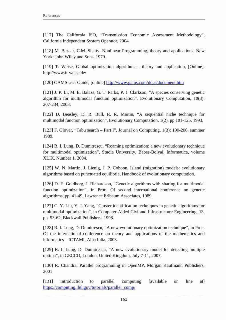
References
162
[117] The California ISO, “Transmission Economic Assessment Methodology”, California Independent System Operator, 2004.
[118] M. Bazaar, C.M. Shetty, Nonlinear Programming, theory and applications, New York: John Wiley and Sons, 1979.
[119] T. Weise, Global optimization algorithms – theory and application, [Online]. http://www.it-weise.de/
[120] GAMS user Guide, [online] http://www.gams.com/docs/document.htm
[121] J. P. Li, M. E. Balazs, G. T. Parks, P. J. Clarkson, “A species conserving genetic algorithm for multimodal function optimization”, Evolutionary Computation, 10(3): 207-234, 2003.
[122] D. Beasley, D. R. Bull, R. R. Martin, “A sequential niche technique for multimodal function optimization”, Evolutionary Computation, 1(2), pp 101-125, 1993.
[123] F. Glover, “Tabu search – Part I”, Journal on Computing, 1(3): 190-206, summer 1989.
[124] R. I. Lung, D. Dumitrescu, “Roaming optimization: a new evolutionary technique for multimodal optimization”, Studia University, Babes-Bolyai, Informatica, volume XLIX, Number 1, 2004.
[125] W. N. Martin, J. Lienig, J. P. Cohoon, Island (migration) models: evolutionary algorithms based on punctuated equilibria, Handbook of evolutionary computation.
[126] D. E. Goldberg, J. Richardson, “Genetic algorithms with sharing for multimodal function optimization”, in Proc. Of second international conference on genetic algorithms, pp. 41-49, Lawrence Erlbaum Associates, 1989.
[127] C. Y. Lin, Y. J. Yang, “Cluster identification techniques in genetic algorithms for multimodal optimization”, in Computer-Aided Civi and Infrastructure Engineering, 13, pp. 53-62, Blackwall Publishers, 1998.
[128] R. I. Lung, D. Dumitrescu, “A new evolutionary optimization technique”, in Proc. Of the international conference on theory and applications of the mathematics and informatics – ICTAMI, Alba Iulia, 2003.
[129] R. I. Lung, D. Dumitrescu, “A new evolutionary model for detecting multiple optima”, in GECCO, London, United Kingdom, July 7-11, 2007.
[130] R. Chandra, Parallel programming in OpenMP, Morgan Kaufmann Publishers, 2001
[131] Introduction to parallel computing [available on line at] https://computing.llnl.gov/tutorials/parallel_comp/

References
163
[132] Centre for Astrophysics and supercomputing http://astronomy.swin.edu.au/supercomputing/
[133] GAMS user Guide, [online] http://www.gams.com/docs/document.htm
[134] E. Hansen, G. W. Walster, Global Optimization Using Interval Analysis: Revised And Expanded (Pure and Applied Mathematics), Dekker publisher, 2007.
[135] University of Washington, College of Engineering website, http://www.ee.washington.edu/research/pstca/