1

On Instantaneous Frequency

By

Norden E. Huang NASA Goddard Space Flight Center

Greenbelt, MD 20771 USA Norden.E.Huang@nasa.gov

Zhaohua Wu

Center for Ocean-Land-Atmosphere Studies Calverton, Maryland 20705-3106 USA

zhwu@cola.iges.org

Steven R. Long NASA Goddard Space Flight Center

Wallops Flight Facility Wallops Island, VA 23337 Steven.R.Long@nasa.gov

March 2006

2

Abstract Instantaneous Frequency (IF) is the necessary quantity for understanding fully the detailed mechanisms involved in nonlinear and nonstationary processes. Historically, IF was computed from the Analytic Signal (AS) through the Hilbert transform. Although the Hilbert transform exists for any L2 class function, computing IF using the AS generated from the Hilbert transform is not straightforward. It is well known that for IF to make physical sense, the function has to be mono-component. Furthermore, there are two theoretical limitations on computing a physically meaningful IF through the Hilbert transform: the Bedrosian and Nuttall theorems: Bedrosian set the limit on clean separation of AM and FM; Nuttall gives necessary condition on phase function fidelity. A new empirical FM and AM (frequency and amplitude modulation) demodulation was proposed to satisfy these limitations. Then IF can be computed exactly by Driect Quadrature (with quadrature defined here as a simple 90° shift of phase angle) on the FM signal. Alternatively IF can be computed through AS from the empirical FM signal. The results thus obtained indicate that the various problems that have been associated with instantaneous frequency determination are now fully resolved, and that a true time-frequency analysis method has taken another step towards maturity.

3

1. Introduction The term ‘Instantaneous Frequency (IF)’ has always elicited strong opinions in the data analysis and communication engineering communities, with comments covering the range from ‘banishing it forever from the dictionary of the communication engineer’ (Shekel, 1953), to being a ‘conceptual innovation in assigning physical significance to the nonlinearly distorted waveforms’ (Huang et al. 1998). Between these two extremes, there are many more moderate opinions stressing the need for and also airing the frustration over finding an acceptable definition and workable way to compute its values. Before discussing any methods for computing IF, the concept of an instantaneous value for the frequency must be justified. After all, the traditional definition of frequency is the inverse of period, and the analysis methods are mostly based on the Fourier transform, which give time invariant amplitude and frequency values. Furthermore, the inherited uncertainty principle associated with the Fourier transform pair has prompted Gröchenig (2001) to say, ‘The uncertainty principle makes the concept of an Instantaneous Frequency impossible.’ Fourier analysis is, however, only one of the mathematic methods; to find a solution to this controversy over IF, methods beyond the Fourier techniques must be considered. Indeed, the need and the fact that the frequency should have instantaneous values can be justified from both mathematical and physical grounds. Mathematically, the commonly accepted definition of frequency in classical wave theory is based on the existence (see, for example, Whitham, 1974; or Infeld and Rowlands, 1990) of ‘slowly’ varying amplitude a(x, t) and phase θ(x, t) functions, such that the wave profile is the real part of the complex valued function, ( )i ( x ,t )( x ,t ) R a( x,t )e .θς = (1) Then it follows that the frequency, ω, and the wave number, k, are defined as

and k .t xθ θω ∂ ∂

= − =∂ ∂

(2)

By cross-differentiating the frequency and wave number, the wave conservation equation immediately follows ,

k 0 .t x

ω∂ ∂+ =

∂ ∂ (3)

This is one of the fundamental laws governing all wave motion. The assumption of the classic wave theory is very general: that the wave motion is given by Equation (1). If frequency and wave number can be defined as in Equation (2), then they have to be differentiable functions of the temporal and the spatial variables for Equation (3) to hold. Thus, for any wave motion, other than the trivial kind of constant frequency sinusoidal motion, the frequency representation should have instantaneous values. Therefore, there

4

should not be any doubt about the mathematical meaning nor the necessity of the existence of IF. The classical wave theory was founded on rigorous mathematical grounds, with many of the theoretical results confirmed by observations (Infeld and Rowlands, 1990). This model can be generalized to all types of wave phenomena, such as surface water waves, acoustics and optics. The pressing questions are how to define the phase function and IF for any given wave data set. Physically, there is also a real need for IF in a faithful representation of underlying mechanisms for data from nonlinear processes. Obviously, the non-stationarity is also one of the key features here, but as explained by Huang et al. (1998), the concept of IF is essential for a physically meaningful interpretation of nonlinear processes. For a non-stationary process, the frequency should be an ever changing measure. Consequently, a time-frequency representation for the data is needed, or in other words, the frequency value has to be a function of time. For nonlinear processes, the frequency variation as a function of time is even more drastic. To illustrate the need for IF in the nonlinear cases, consider the Duffing model,

2

32

d x x x cos t ,dt

ε γ ω+ + = (4)

in which ε is a parameter not necessarily small, and the right hand term is the forcing function of magnitude γ and frequency ω. This cubic nonlinear equation can be re-written as

2

22

d x x ( 1 x ) cos t ,dt

ε γ ω+ + = (5)

where the term in the parenthesis can be regarded as a single quantity representing the spring constant of the nonlinear oscillator, or the pendulum length of a nonlinearly constructed pendulum. As this quantity is a function of position, the frequency of this oscillator is ever changing, even within one oscillation. This intra-wave frequency modulation is the singular most unique characteristics of a nonlinear oscillator, as proposed by Huang et al. (1998, 1999). The geometric consequence of this intra-wave frequency modulation is the observed waveform distortion. Traditionally, such nonlinear phenomena are represented by of the fundamental wave and its harmonics in Fourier analysis, and it is thus viewed as harmonic distortion. This traditional view, however, is the consequence of imposing a linear structure on a nonlinear system: the superposition of simple harmonic functions with each as a solution for a linear oscillator. One can only assume that the sum and total of the linear superposition would give an accurate representation of the fully nonlinear system; all of the individual harmonic terms, however, are mathematical artifacts and have no physical meaning. For example, in the case of water surface waves, such harmonics are not free physical waves satisfying the dispersive relationship (Huang et al., 1999). Although, this perturbation approach seems to have worked well for systems with infinitesimal nonlinearity, the approach fails when the nonlinearity is finite and the motion becomes chaotic (see, for example, Kantz and Schreiber, 1997). A natural and logical approach should be one that can capture the

5

essence, such as being able to describe the nonlinear system as behaving like an oscillator with variable frequency, assuming different values at different times, even within one single period. To describe such a motion, IF is essential. In the real world of experimental and theoretical studies, the conditions of ever changing frequency are common, if not actually prevailing. A chirp signal is one class of these signals, used by bats as well as in radar. The frequency content in speech, though not exactly chip, is also ever changing. And many of the consonants used in spoken language are produced through highly nonlinear but natural mechanisms, such as explosion or friction. Furthermore, for any nonlinear system, the frequency is definitely modulating not only among different oscillation periods, but also within one period as discussed above. The true physical processes must be examined through IF from non-Fourier based methods. There are copious publications in the past on IF, for example: Boashash (1992 a, b, c), Kootsookos et al (1992), Lovell et al. (1993), Cohen (1995), Flandrin (1995), Loughlin and Tracer (1996) and Picinbono (1997). Most of these publications, however, were concentrated on the Wigner-Ville Distribution (WVD) and it variations, where IF is defined through the mean moment of different components at a given time. But there are no a priori reasons to assume that the multi-component signal should have a single-valued instantaneous frequency at any given time while still retaining full physical significance. Other than the Wigner-Ville distribution, instantaneous frequency through the Analytic Signal (AS) produced by the Hilbert transform has also received much attention. These points will be discussed in more detail later. One of the most basic, yet confusing, points concerning Instantaneous Frequency is the erroneous idea that for each instantaneous frequency value there must be a corresponding frequency in the Fourier Spectrum of the signal. In fact, instantaneous frequency of a signal when properly defined should have very different meanings compared with the frequency in the Fourier spectrum, as discussed in Huang et al. (1998). But the divergent and confused viewpoints on IF indicate that the erroneous view is a deeply rooted one, associated with and responsible for some of the current misconceptions and fundamental difficulties in computing IF. Some of the traditional objections on IF can actually be traced to the mistaken assumption that a single-valued IF exists for any function at any given instant. Instantaneous frequency witnessed two major advances recently through the introduction of the Empirical Mode Decomposition (EMD) method and the Intrinsic Mode Function (IMF) introduced by Huang et al. (1998) for data from nonlinear and nonstationary processes, and alternatives by Wavelet based decomposition and more generalized demodulation introduced by Olhede and Walden (2004 and 2005) for data from linear nonstationary processes. Huang et al. (1999) have also introduced the Hilbert view on nonlinearly distorted waveforms, which provided explanations to many of the paradoxes raised by Cohen (1995) on the validity of the IF, which will also be discussed in details later. Indeed, the introduction of EMD or the generalized demodulation method resolved one key obstacle for computing a meaningful IF from a multi-component signal by

6

reducing it to a collection of mono-component functions. Once the mono-component functions are obtained, there are still limitations on applying the AS for physically meaningful instantaneous frequency as stipulated by the well-known Bedrosian (1963) and Nuttall (1966) theorems. Some of the mathematical problems associated with the Hilbert transform of IMFs have also been addressed by Vatchev (2004). In this paper, an empirical AM and FM demodulation (Huang, 2003) is proposed based on a spline fitted normalization scheme to produce a unique and smooth empirical envelope (AM) and a unity valued carrier (FM). Experience indicates that the empirical envelope so produced is identical to the theoretical one when explicit expressions exist, and it provides a smoother envelope than any other method including the AS approach when there are no explicit expressions for the data. The spline based empirical AM and FM demodulation will not only remove most of the difficulties associated with the AS, but also enables the quadrature (defined as 90° phase shift) to be directly computed. It follows that the IF can then be computed through the direct quadrature function (DQ) without any approximation. The normalization also resolves many of the traditional difficulties associated with an IF computed through the AS: It makes the AS satisfy the limitation imposed by the Bedrosian theorem (Bedrosian, 1963) so that the IF is not influened by the AM variations. At the same time, it provides a sharper and more easily computable error index than the one proposed by the Nuttall theorem (Nuttall, 1966), which gives the error bound when the Hilbert transform of a function is different from its quadrature. Additionally, alternative methods based on a generalized zero-crossing and an energy operator will be introduced to define frequency locally for cross comparisons. 2. Definitions of Frequency Frequency is an essential quantity in the study of any oscillatory motion. The most fundamental and direct definition of frequency, ω, is simply the inverse of period, T; that is

1 .T

ω = (6)

Following this definition, the frequency exists only if there is a whole cycle of wave motion. And the frequency would be constant over this length, with no finer temporal resolution. In fact, a substantial number of investigators still hold the view that frequency cannot be defined without a whole wave profile. Equation (6) suggests that the way of determining the frequency is to measure the time intervals between consecutive zero-crossings or the corresponding points of the phase on successive waves. This is very easily implemented for a mono-component wave train, where the period is well-defined. However for real data, this restrictive view presents several difficulties: To begin with, the fundamental wave conservation law requires the wave number and frequency to be differentiable. How can the frequency be differentiable if its value is constant over a whole wavelength? Secondly, this view

7

cannot reveal the detailed frequency modulations observed with ever changing frequency in nonstationary and, especially, nonlinear processes with intra-wave frequency modulations. And finally, in a complicated vibration, there might be multi-extrema between two consecutive zero-crossings, a problem treated extensively by Rice (1944a,b and 1945a,b), who restricted the application of the zero-crossing method to narrow band signals, where the signal must have equal numbers of extrema and zero-crossings. Therefore, without a procedure like the EMD to decompose the data into IMFs, this simple zero-crossing method has only been used for band-passed data (see, for example, Melville, 1983), or more recently by the sophisticated and generalized demodulation by Olhede and Walden (2004, 2005). As the band-pass filters used all work in frequency space, they tend to separate the fundamental from its harmonics; the filtered data will thus loose most, if not all, of its nonlinear characteristics. With these difficulties, it follows that the zero-crossing method has seldom been used in serious research work. Another definition of frequency is through the dynamic system using the variation of the Hamiltonian, H(q, p), where q is the generalized coordinate, and p, the generalized momentum (see, for example, Goldstein, 1980; or Landau and Lifshitz, 1976) as,

H( A )( A ) ,A

ω ∂=

∂ (7)

in which A is the action variable defined as A pdq= ∫ , (8) where the integration is over a complete period of a rotation. The frequency so defined is varying with time, but the resolution is no finer than the averaging over one period, for the action variable is an integrated quantity, as given in Equation (8). Thus the frequency defined by Equation (7) is equivalent to the inverse of the period, which is the classical definition of frequency. This method is elegant theoretically, but its utility is limited to relatively simple low dimensional dynamic systems, linear or nonlinear, whenever integrable solutions describing the full process exist. Consequently, it cannot be routinely used for data analysis. In practical data analysis, the data is a real variable, which may have multi-extrema between consecutive zero-crossings. There can also be many coexisting frequency values at any given time. Traditionally, the only way to define frequency is to find its content in a data set that is computed through the Fourier transform. Thus, for a time series, x(t), this is just

jN

i tj

j 1x( t ) R a e ,ω−

=

= ∑ (9)

where

8

j

Ti t

jo

a x( t ) e dt ,ω= ∫ (10)

with R indicating the real part of the quantity. With classic Fourier analysis, the frequency values are constant over the whole time span covering the range of the integration. As the Fourier definition of frequency is not a function of time, it can easily be seen that the frequency content would be physically meaningful only if the data represent a linear (to allow superposition) and stationary (to allow a time independent frequency representation) process. A slight generalization of the classic Fourier transform is to break the data into short sub-spans. Thus the frequency value can still vary globally, but can then be assumed to be constant locally within each sub-integral time span. Nevertheless, the integrating operation leads to the uncertainty principle, which imposes the fundamental limitation on this Fourier type of analysis.. At any rate, the uncertainty principle dictates that the Fourier type methods can not possiblly resolve a signal with its frequency varying faster than the integration time scale, certainly not within one period (Gröchenig, 2001). A further generation of the Fourier transform approach is Wavelet Analysis, a very popular data analysis method (see, for example, Daubechies, 1992, and Percival and Walden 2000), which is also extremely useful for data compression, and image edge definitions, for example. True, wavelet analysis offers time-frequency information with an adjustable window. The most serious weakness of wavelet analysis is again the limitation of the uncertainty principle: To be local, a base wavelet cannot contain too many waves; to have fine frequency resolution, a base wavelet will have to contain many waves. The frequency resolution problem is mitigated greatly through the Hilbert spectral representation (Olhede and Walden (2004, 2005). Nevertheless, these improved methods are physically meaningful when the data are from nonstationary but linear processes. Yet another variation of the classical Fourier analysis can be found in the Wigner-Ville distribution (see, for example, Cohen, 1995), which is defined as

* iV ( t , ) x t x t e d .2 2

ωττ τω τ∞

−

−∞

⎛ ⎞ ⎛ ⎞= + −⎜ ⎟ ⎜ ⎟⎝ ⎠ ⎝ ⎠∫ (11)

By construction, the marginal distribution (obtained by integrating out the time variable) is identical to the Fourier power density spectrum. Even though the full distribution does offer some time-frequency properties, it can only provide a center of gravity type of weighted mean local frequency as

9

V ( t , )d

( t ) .V ( t , )d

ω ω ωω

ω ω

∞

−∞∞

−∞

⎛ ⎞⎜ ⎟⎝ ⎠=⎛ ⎞⎜ ⎟⎝ ⎠

∫

∫ (12)

Here only a single value is the mean for all the different components. This mean value lacks the necessary detail needed to describe the complexity imbedded in a multi-component data set. It should be noted that all the above methods work for any data, while the methods to be discussed in the next section work only for mono-component functions. 3. Instantaneous Frequency Ideally, IF for any mono-component data should be calculated through its quadrature, defined as a simple 90o phase shift of the carrier phase function. Let the mono-component data be expressed by its envelope, a(t), and carrier, cos ( )tφ , as x( t ) a( t ) cos ( t )φ= , (13) where ( )tφ is the phase function. Its quadrature then is xq( t ) a( t ) sin ( t )φ= , (14) no matter how complicated the amplitude and phase functions are. With these expressions, IF can be computed as in the classical wave theory given in Equation (2). These seemingly trivial steps have been impossible to implement in the past. To begin with, not all the data from real processes are mono-component. Even though methods for decomposing the data into a collection of mono-component functions are now available (Olhede and Walden, 2004 and 2005), data from nonlinear processes should be decomposed by the Empirical Mode Decomposition (Huang, et al., 1998.). Associated with the EMD are other daunting difficulties: to find the unique pair of [a(t), ( )tφ ] representing the data, and to find a general method to compute the quadrature directly. Traditionally, the accepted way is to use the AS through Hilbert transform (HT) as a proxy for the quadrature. This has made the AS approach the most popular method to define Instantaneous Frequency. The most fundamental difficulty of the AS approach is that it offers only an approximation to the quadrature, except for some very simple cases. Due to this and other difficulties associated with this approach, it has also contributed to all the controversies related to IF. To fully appreciate the subtlety of IF defined through HT, a brief history of IF is necessary. A more detailed one can be found in Boashash (1992 a and b), for example. For the sake of completeness and to facilitate the discussions,

10

certain essential historical milestones of the approach will be traced from its beginning to its present state, as follows: The first important step in defining instantaneous frequency was due to Van der Pol (1946), a pioneer in nonlinear system studies, who first seriously explored the idea of instantaneous frequency. He proposed the correct expression of the phase-angle as an integral of IF. The next important step was made by Gabor (1946), who introduced the Hilbert transform to generate a unique analytic signal (AS) from real data, thus removing the ambiguity of the infinitely many possible amplitude and phase pair combinations to represent the data. Gabor’s approach is summarized as follows: For the variable x(t), its Hilbert transform, y(t), is defined as

1 x( )y( t ) P d ,tτ

τ τπ τ

=−∫ (15)

with P indicating the Cauchy principal value of the complex integral. The Hilbert transform provides the complex conjugate, y(t), of the real data. Thus, a unique Analytic Signal is given by i ( t )z( t ) x( t ) i y( t ) A( t ) e ,θ= + = (16) in which

{ }1 / 22 2 1 y( t )A( t ) x ( t ) y ( t ) , and ( t ) tan ,x( t )

θ −= + = (17)

form the canonical pair, [A(t), θ(t)], associated with x(t). Gabor even proposed a direct method to obtain the AS through two Fourier transforms:

i t

0

z( t ) 2 F( ) e d ,ωω ω∞

= ∫ (18)

where, F(ω) is the Fourier transform of x(t). In this representation, the original data x(t) becomes { }i ( t )x( t ) R A( t )e A( t ) cos ( t ) .θ θ= = (19) It should be pointed out that this canonical pair, [A(t), θ(t)], is in general different form the complex number defined by the quadrature, [a(t), ( )tφ ], though their real parts are identical. For the analytic pair, IF can be defined as the derivative of the phase function of the complex pair given by

11

( )2

d ( t ) 1( t ) x y' y x' .dt Aθω = = − (20)

For stochastic data, the phase function in general is a function of time; therefore, IF is also a function of time. This definition of frequency bears a striking similarity with that of the classical wave theory. As the Hilbert transform (HT) exists for any function of L2 class, there is a misconception that one can put any function through the above operation and obtain a physically meaningful instantaneous frequency as advocated by Hahn (1995). Such an approach has instead created great confusion over the meaning of IF in general, and tarnished the approach of using the Hilbert transform for computing IF in particular. The most obvious fallacy of this approach is that the IF values from the multi-component data would have scattered over a wide range. These values are not physically meaningful at all, instantaneously or otherwise. The difficulties encountered here actually can be illustrated by a much simpler example using the function employed by Huang et al. (1998): x( t ) a cos tα= + , (21) with a as an arbitrary constant. Its Hilbert transform is simply y( t ) sin tα= ; (22) therefore, IF according to Equation (20) is

( )a sin t

a cos t aα α

ωα

+=

+ + 2

11 2

. (23)

Equation (23) can give any value for IF, depending on the value of a. In order to recover the frequency of the input sinusoidal signal, the constant has to be zero. This simple example illustrates some crucial necessary conditions for the AS approach to give a physically meaningful IF: The function will have to be mono-component, with a zero mean locally, and the wave will have to be symmetric with respect to the zero mean. All these conditions are satisfied by either the EMD or wavelet projection methods mentioned above. But these are only the necessary conditions. There are other more subtle and stringent conditions for the AS approach to be able to produce a meaningful IF. For example, Loughlin and Tracer (1996) proposed physical conditions for the AM and FM of a signal in order for the IF to be physically meaningful, and Picinbono (1997) proposed spectral properties of the envelope and carrier in order to have a valid AS representation. Indeed, the unsettling state of the AM and FM demodutation, and the associated instantaneous frequency have created great misunderstanding, and that has prompted Cohen (1995) to list a number of ‘paradoxes’ concerning IF. Some of the paradoxes concerning negative frequency are direct consequences of these necessary conditions given by the IMFs. All the paradoxes will be discussed in turn.

12

In fact, the most general conditions are already summarized most succinctly by the Bredrosian (1963) and Nuttall (1966) theorems. Bedrosian (1963) established another general necessary condition for obtaining meaningful IF values from AS, which set a limitation on the clean separation of the AM and FM parts through the Hilbert transform: { } { }H a( t )cos ( t ) a( t ) H cos ( t ) ,θ θ= (24) provided that the Fourier spectra of the envelope and the carrier are non-overlapping. This is a much sharper condition on the data: the data has to be not only mono-component but also narrow band, otherwise the AM variations will contaminate the FM part. The IMF produced by the EMD does not satisfy this requirement automatically. With the spectra from amplitude and carrier not clearly separated, IF will be influenced by the AM variations. As a result, the applications of the Hilbert transform as used by Huang et al. (1998, 1999) are still plagued by occasional negative frequency values. Strictly speaking, unless one uses band-pass filters, any local AM variation will violate the restriction of the Bedrosian theorem. If any data violate the condition set forth in Equation (24), the operations given in Equation (16) to (20) will no longer be valid. Although an AS can still be obtained with the real part identical to the data, the imaginary part would not be the same through the effect on the phase function contaminated by the amplitude modulations. In reality, the Bredrosian condition is not the only problem. More fundamentally, Nuttall (1966) questioned the condition under which one can write { }H cos ( t ) sin ( t ) ,φ φ= (25) for an arbitrary function of ( )tφ . The critical idea here is to preserve the true phase function as defined through the quadrature. This difficulty has been ignored by most investigators using the Hilbert transform to compute IF. Picinbono (1997) stated that it would be impossible to justify Equation (25) from only the spectral properties. He then entered an extensive discussion on the specific properties of the phase function under which Equation (25) would be true. The conditions were recently generalized by Qian et al. (2005) and Chen et al. (2005). But such discussions would be of very limited practical use in data analysis, for the data cannot be forced to satisfy the conditions prescribed. Picinbono finally concluded that ‘the only scientific procedure would require the calculation of the error coming from the approximation’, which resides only in the imaginary part of the AS. He also correctly pointed out that there is no general procedure to calculate this error from the spectrum of the amplitude function, for the error depends on the structure of the phase function rather than on spectral properties of the amplitude function. Faced with the difficulties presented by Picinbono (1997), only the partial solution provided by the Nuttall (1966) theorem is available. Nuttall (1966) first established the following theoretical result: For any given function x( t ) a( t ) cos ( t ) ,φ= (26)

13

for arbitrary a(t) and ( )tφ that are not necessarily narrow band functions, and if the Hilbert transform of x(t) is given by xh(t), and the quadrature of x(t) is xq(t), then

[ ]0

2q

t

E xh( t ) xq( t ) dt 2 F ( )d ,ω

ω ω∞

=−∞ −∞

= − =∫ ∫ (27)

where

i tqF ( ) F( ) i a( t ) sin ( t ) e dt ,ωω ω θ

∞−

−∞

= + ∫ (28)

in which F(ω) is the spectrum of the signal, and Fq(ω) is the spectrum of the quadrature of the signal. Therefore, the necessary and sufficient conditions for the Hilbert transform and the quadrature to be identical is E = 0. This is an important and brilliant result, yet not very practical and useful. The difficulties are due to the following three deficiencies: First, the result is expressed in terms of the quadrature spectrum of the signal, which is an unknown quantity, if quadrature is unknown. Second, the result is given as an overall integral, which provides a global measure of the discrepancy. Finally, the error index is energy based; it only states that the xh(t) and xq(t) are different, but does not offer an error index on the frequency (Picinbono, 1997). Therefore, the Nuttall theorem offers only a proxy for the error index of IF; it is again a necessary condition for the AS approach to yield the exact IF. These difficulties, however, do not diminish the significance of Nuttall’s result: it points out a serious problem and limitation on equating the Hilbert transform and the quadrature of a signal; therefore, there is a serious problem on using the Hilbert transform to compute physically valid instantaneous frequency values. All these important results were known by the late 1960s. For lack of a satisfactory method to decompose the data into the mono-component functions other than the traditional band-pass filters, the limitations set by Bedrosian and Nuttall were irrelevant, for the band-passed signal is linear and narrow band and satisfies the limitation automatically. As it is also well known that band-passed signals would eliminate many interesting nonlinear properties for the data, the band-pass approach could not make the Hilbert transform generated the AS as a general tool for a physically valid instantaneous frequency computation. Consequently, the HT method still remains as an impractical method for data analysis. The solutions to these various difficulties are presented in the next section. 3.1 The Normalization Scheme : An Empirical AM and FM Demodulation Both limitations stated by the Bedrosian and Nuttall Theorems have firm theoretical foundations, and must be satisfied. To this end, an empirical AM and FM demodulation method is proposed, which is an iterative normalization scheme enabling any IMF to be

14

separated empirically and uniquely into envelope (AM) and carrier (FM) parts. This normalization demodulation scheme has three important consequences: First and most importantly, the normalized carrier enables the direct computation of quadrature (DQ). Second, the normalized carrier has unity amplitude; therefore, it satisfies the Bedrosian theorem automatically. Finally, the normalized carrier enables a ready and sharper local energy-based measure of error to be provided than that given by the Nuttall theorem. When the empirical AM and FM demodulation through the normalization scheme is used in conjunction with the AS, it is designated in this study as the Normalized Hilbert Transform (NHT). Other than the direct quadrature (DQ) and NHT, two additional methods will also be introduced for determining the local frequency independently of the Hilbert Transform: each based on different assumptions, and each giving slightly different values for IF from the same data. For all of these methods to work, the data will have to first be reduced to an IMF. As this empirical AM and FM demodulation is of great importance to the subsequent discussions, it will be presented first as follows: First, from a given IMF data set in Figure 1.1, identify all the local maxima of the absolute value of the data, as shown in Figure 1.2. By using the absolute value fitting, the normalized data are guaranteed to be symmetric with respect to the zero axis. Next, all these maxima points are connected with a cubic spline curve. This spline curve is then designated as the empirical envelope of the data, e1(t), also shown in Figure 1.2. In general, this envelope is different from the modulus of the AS. For any given real data, the extrema are fixed; therefore, this empirical envelope should be fixed and uniquely defined without any ambiguity. Having obtained the empirical envelope through spline fitting, this envelope can then be used to normalize the data, x(t), by

11

( )( )( )

x ty te t

= , (29)

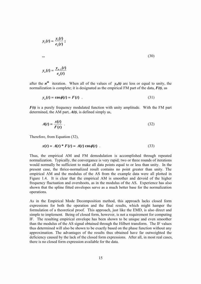
with y1(t) as the normalized data. Ideally, y1(t) should have all of its extrema with a unity value. Unfortunately, Figure 1.3 shows that the normalized data still have amplitudes higher than unity occasionally. This is due to the fact that the spline is fitted through the maximum points only. At the locations of fast changing amplitudes, the envelope spline line, passing through the maxima, can go below some data points. Even with these occasional flaws, the normalization scheme has effectively separated the amplitude from the carrier oscillation. To remove any occasional flaw of this type, the normalization procedure can be implemented repeatedly, with e2(t) defined as the empirical envelope for y2(t) and so on as,

15

12

2

1

( )( ) ;

( )

...

( )( )

( )n

nn

y ty t

e t

y ty t

e t−

=

=

(30)

after the nth iteration. When all of the values of yn(t) are less or equal to unity, the normalization is complete; it is designated as the empirical FM part of the data, F(t), as ( ) cos ( ) ( )ny t t F tφ= = . (31) F(t) is a purely frequency modulated function with unity amplitude. With the FM part determined, the AM part, A(t), is defined simply as,

( )( )( )

x tA tF t

= . (32)

Therefore, from Equation (32), ( ) ( ) * ( ) ( ) cos ( )x t A t F t A t tφ= = . (33) Thus, the empirical AM and FM demodulation is accomplished through repeated normalization. Typically, the convergance is very rapid; two or three rounds of iterations would normally be sufficient to make all data points equal to or less than unity. In the present case, the thrice-normalized result contains no point greater than unity. The empirical AM and the modulus of the AS from the example data were all plotted in Figure 1.4. It is clear that the empirical AM is smoother and devoid of the higher frequency fluctuation and overshoots, as in the modulus of the AS. Experience has also shown that the spline fitted envelopes serve as a much better base for the normalization operations. As in the Empirical Mode Decomposition method, this approach lacks closed form expressions for both the operation and the final results, which might hamper the formulation of a theoretical proof. This approach, just like the EMD, is also direct and simple to implement. Being of closed form, however, is not a requirement for computing IF. The resulting empirical envelope has been shown to be unique and even smoother than the modulus of the AS signal obtained through the Hilbert transform. The IF values thus determined will also be shown to be exactly based on the phase function without any approximation. The advantages of the results thus obtained have far outweighted the deficiency caused by the lack of the closed form expressions. After all, in most real cases, there is no closed form expression available for the data.

16

It should be noted here that the normalization process could cause some deformation of the original data, but the deformation is negligible, for there are rigid controlling points for the periodicity provided by the zero-crossing points in addition to the extrema. The zero-crossing points are totally un-alternated by the normalization process. As discussed above, an alternative method to normalize an IMF is to use the modulus of the AS instead of the spline envelope in the normalization scheme. This will certainly avoid the problem of the envelope dipping under the data, but any nonlinear distorted wave form will give a jagged AS modulus envelope, which could in turn cause an even worse deformation of the waveforms in the normalized data. 3.2 Direct Quadrature (DQ) Having proposed the empirical AM and FM demodulation, the normalized IMF can be used as a base to compute its quadrature directly. This approach will eschew the Hilbert transform totally, and enable the calculation of an exact instantaneous frequency. After the normalization, the empirical FM signal, F(t), is the carrier part of the data. Assuming the data to be a cosine function, its quadrature is given simply as, 2sin ( t ) 1 F ( t )φ = − . (34) In computing the quadrature, the sign should be assumed to be both positive and negative, according to the four-quadrant convention. The complex pair formed by the data and its direct quadrature is not necessarily analytic. They are computed solely to preserve the correct phase function without the kind of distortion as found in the AS approach. There seems to be many advantages in this direct quadrature approach: it bypasses the transform totally; therefore, it involves no question about the integral interval. Its value is also not influenced by any neighboring points. The frequency computation is based only on differentiation; therefore, it is as local as any method can be. Furthermore, without any transform, it preserves the phase function of any data exactly. Once the quadrature is in hand, there are two possible ways to compute the phase from the FM signal: One possibility is to compute the phase angle by simply taking the arccosine of the empirical FM signal as given in Equation (31) directly. Another way is to use arctangent to calculate the phase angle as

21

F ( t )( t ) arc tanF ( t )

φ =−

. (35)

Here F(t) has to be a perfectly normalized IMF after repeated iterations of normalization. This is very critical, for any value of the normalized data that goes beyond unity will cause the formula given in Equation (34) to become imaginary, and Equation (35) to breakdown.

17

Though the arccosine and arctangent approaches are mathematically equivalent, they are computationally slightly different. In both approaches, proper unwrapping is required so as to obtain well defined phase angles that are not limited to piecewise values between 0 to π for arccosine or –π/2 to π/2 for arctangent, along the time axis. Experience with different computational platforms shows that calculations using a four-quadrant arctangent or angle of data and its quadrature pair lead to relatively fewer chances of dramatically unrealistic values of phase angle changes along two consecutive data points which are at or near the extremas, as compared to using arccosine. However, both methods still result in identifiable artificial IFs at the extremas and their close neighborhoods. To alieviate these distortions, the IFs at the extremas (and their close neighbors with the absolute value of F(t) larger than a prescribed critical value, e.g., 0.99) are left to be determined by spline fitting with known IFs to interpolate and/or extrapolate the undefined IFs. This approximation not only reduces the high sensitivity of the calculated phase angles to inaccurate numerical values of F(t) at extremas and their close neighbors, but also eliminates most of the errors in IFs induced by the slight shift of the locations of extremas during the normalization process discussed earlier Although both arccosine and arctangent methods are almost equally effective, in all the subsequent computations, the arctangent approach will be used as the default operation in the Direct Quadrature method unless otherwise noted. IF computed from the direct quadrature (DQ) is given in Figure 1.5, together with the NHT method that will be discussed later. Here the improvement of the DQ is clearly shown: the initial negative IF values disappeared from the simple non-normalized AS at the amplitude minimum. These negative frequency values, near the neighborhood of this minimum amplitude location, are the consequence of violating the condition stipulated by the Bedrosian theorem. By definition, the energy-based error index as defined by Nuttall would be zero identically. The DQ gives the correct phase functions even for data with extremely complicated phase functions. In most cases, however, the numerical difference between the direct quadrature (DQ) and the HT is small, as shown in Figure 1.5. 3.3 Normalized Hilbert Transform (NHT) As the amplitude of the empirical FM signal is identically unity, the limitation of the Bedrosian Theorem is no longer a concern in computing the AS through the Hilbert transform. IF computed from the normalized data is also given in Figure 1.5. Here the improvement of the normalization scheme is also seen clearly: the initial negative IF values were eliminated from non-normalized data near the amplitude minimum locations, for the condition stipulated by the Bedrosian theorem is satisfied automatically. The only noticeable differences between the NHT and DQ approach all occur near where the waveform suffers some distortion. Such distortions are due to the condition stipulated by the Nuttall theorem, for the NHT can only give an approximate answer. If the Hilbert transform indeed produces the quadrature, then the modulus of the AS from the FM signal should be unity. Any deviation of the modulus of the AS from unity is the

18

error; thus this gives an energy-based indicator of the difference between the quadrature and the Hilbert transform, which can be now defined simply as ( ) 2

E( t ) abs analytic signal ( z( t )) 1 .⎡ ⎤= −⎣ ⎦ (36) This error indicator is also a function of time, as shown in Figure 1.6; it gives a local measure of the error incurred in the amplitude, but not of IF computation directly (Picinbono, 1997). Nevertheless, this surrogate measure of error is both logically and practically superior to the integrated error bound established by the Nuttall Theorem. If the quadrature pair and the AS are identical, then the error should be zero. However, they usually are not identical. Based on experience, the majority of the error comes from the following two sources: The first source is due to data distortion in the normalization at locations near drastic changes of amplitude, where the envelope spline fitting will not be able to turn sharp enough to cover all the data, but will go under some data points. A repeated normalization will remove the imperfection in this normalization, but it would inevitably distort the wave profile, for the original location of the extrema could be shifted in the process. This difficulty is even more severe when the amplitude is also locally small, where any error will be amplified by the smallness of the amplitude used in the normalization process in Equation (30). The error index from such conditions is usually extremely large. The second source is due to the nonlinear waveform distortion, which will cause a corresponding variation of the phase function, ( )tφ , as stipulated by the Nuttall theorem. As discussed in Hahn (1995) and Huang et al. (1998), when the phase function is not an elementary function, the phase function from the AS and that from the DQ would not be the same. This is the condition stipulated by the Nuttall theorem. The error index from this condition is usually small. Based on experience, both the NHT and DQ methods can be used routinely to give valid instantaneous frequency. The advantage of the NHT is that it has a slightly better computational stability than the direct quadrature method, but the DQ approach certainly gives a more accurate IF under any circumstance. 3.4 Teager Energy Operator (TEO) The Teager Energy Operator (TEO, see, for example, Kaiser, 1990, or Quatieri, 2002) has been proposed as a method to compute instantaneous frequency without involving integral transforms; it is totally based on differentiations. The idea is based on a signal of the form, x( t ) a sin t ,ω= (37) with an energy operator then defined as 2( x ) x x xψ = −& && , (38)

19

where the over-dots represent first and second derivatives of x(t) with respect to time. Physically, if x represents displacement, the operator, ψ(x), is the sum of the kinetic and potential energy, hence the method is designed as the Teager Energy Operator. For this simple oscillator with a constant amplitude and frequency, it follows that 2 2 2 4( x ) a ; and ( x ) a .ψ ω ψ ω= =& (39) By simply manipulating the two terms in Equation (39),

( x ) ( x ); and a .( x ) ( x )

ψ ψωψ ψ

= =&

& (40)

Thus one can obtain both the amplitude and frequency with the energy operator. Kaiser (1990) and Maragos et al. (1993 a, b) have proposed to extend the energy operator approach to the continuous functions of the AM and FM signals, where both the amplitude and the frequency are functions of time. In those cases, the energy operator will offer only an approximation. A distinct advantage of the energy operator is its superb localization property..No integral transform is needed as in the Fourier or Hilbert transforms. The shortcomings of the method are also obvious: the method only works for mono-component functions; therefore, before an effective decomposition method is available, the application of the method is limited to band-pass data only. Even more fundamentally, the method is based on a linear model for a single harmonic component only; therefore, the approximation produced by the energy operator method will deteriorate and even break down when the wave profiles have any intra-wave modulations, or harmonic distortions. In the past, the TEO has only been applied to the Fourier band-passed signals. As a result, the difficulty with the nonlinear distorted waveform was not assessed at all. Having employed the EMD to produce the IMF, the TEO can be tested on nonlinear data for the first time. The very shortcoming of a breakdown caused by the nonlinear distortion, however, makes the TEO a very nice nonlinearity detector. 3.5 Generalized Zero-Crossing (GZC) Any zero-crossing method is the most fundamental method for computing local frequency, and it has long been used to compute the mean period or frequency for narrow band signals (Rice, 1944a,b and 1945a,b). In GZC, the temporal resolution will be improved to a quarter wave period by taking all zero-crossings and local extrema as the critical points. The time intervals between all the combinations of critical points are considered as a whole or partial wave period. For example, the period between two consecutive up (or down) zero-crossings or two consecutive maxima (or minima) can be counted as one whole period. Each given point along the time axis will have four different values from this class of period, designed as T4j , where j=1 to 4. Next, the period between consecutive zero-crossings (from up to the next down zero-crossing, or from down to the next up zero-crossing), or consecutive extrema (from maximum to the next minimum, or from minimum to the next maximum) can be counted as a half period.

20

Each given point along the time axis will have two different values from this class of period, designed as T2j, where j=1 to 2. Finally, the period between one kind of extrema to the next zero-crossings, or from one kind of zero-crossings to the next extrema can be counted as a quarter period. Each given point along the time axis will have only one value from this class of period, designed as T1. Clearly, the quarter period class, T1, is the most local, so it is thus given here a weight factor of 4. The half period class, T2, is the less local, so it in turn is given a weight factor of 2. And finally, the full period class, T4, is the least local, so it is given it a weight factor of 1. In total, at any point along the time axis, seven different period values will be produced, each weighted by their properties of localness. By the same argument, each place will also have seven correspondingly different amplitude values. The mean frequency at each point along the time axis can be computed as

2 4

j 1 j 11 2 j 4 j

1 1 1 1 ,12 T T T

ω= =

⎛ ⎞= + +⎜ ⎟⎜ ⎟

⎝ ⎠∑ ∑ (41)

and the standard deviation can also be computed accordingly. This approach is based on the fundamental definition of frequency given in Equation (6); it is the most direct, and also gives the most accurate and physically meaningful mean local frequency: It is local down to a quarter period (or wavelength); it is direct and robust and involves no transforms or differentiations. Furthermore, this approach will also give a statistical measure of the scattering of the frequency value. The weakness of the approach is its crude localization, only down to a quarter wavelength at most. Another drawback is its inability to represent the detailed waveform distortion, for it admits no harmonics and no intra-frequency modulations. Unless the waveform contains asymmetries (either up and down, or left and right), the GZC will give it the same frequency as a sinusoidal wave. With all these advantages and limitations, for most of the practical applications, however, this mean frequency localized down to a quarter wave period is already better than the widely used Fourier spectrogram. This method is extremely easy to implement, once the data is reduced to a collection of IMFs. In the subsequent comparisons, the GZC results will be used as the baseline reference. Any method producing a frequency or amplitude grossly different from the GZC result in the mean simply cannot be correct. Therefore, the GZC offers a standard reference in the mean for validating the other methods. 4. Inter-comparisons of Results from Different Methods and Discussions Two examples will be used, in order to illustrate the difference in the instantaneous frequencies produced by the different methods. The first example is a model function to illustrate details and the potential problems of the methods; the second example is a real speech signal, which will give an illustration of how the various methods perform in practical applications.

21

The first example is the modeled damped Duffing wave with chirp frequency. The explicit expression of the model gives the truth as a reference and enables the calibration and validation of the methods quantitatively. The model is given by

2 2t t tx( t ) exp cos 32 0.3 sin 32 ,256 64 512 32 512

with t 0 : 1024 .

π π⎛ ⎞⎛ ⎞ ⎛ ⎞⎛ ⎞= − + + +⎜ ⎟⎜ ⎟ ⎜ ⎟⎜ ⎟⎝ ⎠ ⎝ ⎠ ⎝ ⎠⎝ ⎠

= (42)

Assuming the sampling rate to be 1 Hz, the numerical values of the signal are plotted in Figure 2.1. As the amplitude is decaying exponentially, the data must be normalized using the method described in Equation (30). From the normalized data, the quadrature can be computed. The computed quadrature and the imaginary part of the AS were shown in Figure 2.2. The computed quadrature is exactly the same as the one given by the theoretical expression. This offers a clear validation of the direct quadrature computation method (DQ). As the Hilbert transform is implemented through the Gabor (1946) method, the effect of the jump in values at the beginning and the end is clearly visible. The normalized data has corrected the effect of the jump condition. It is important to point out that, for this Duffing model, the quadrature and the AS are not identical, as shown vividly in this figure. Therefore, problems should be anticipated for any IF computed from the AS methods. The phase function of the quadrature is given by a perfect unity circle if the complex phase function were plotted. But the amplitude of the AS from the Hilbert transform will deviate from the unity circle systematically. This deviation results in an energy measure of the error in using the AS as an approximation for the quadrature. To examine the effect of the Bedrosian theorem in detail, the Fourier power spectra was computed for both the AM and FM signals as given in Figure 2.3. Although the AM signal is a monotonic exponentially decaying function, the power spectral density would treat it as a ‘saw-tooth’ function, and thus have a wide spectrum. Therefore, the spectra of the AM and FM signals are not disjoint at all. Consequently, the phase function of the AS will be contaminated by the amplitude variations, for they violate the Bedrosian theorem. As will be seen later, the spectra from the AM and FM signals of an IMF would never be disjoint in general, unless the signals are separated specifically by a band-pass filter. The small but non-zero overlap indicates that the FM part of the AS generated through the Hilbert transform is always an approximation that is contaminated by the AM variations. Now, IF values given in Figure 2.4 will be examined. Here again, the IF from the DQ method coincides with the theoretical values exactly. To examine the discrepancy in detail, one would see that the IF values from DQ show some deviation from the true theoretical ones near the peaks of each wave, towards the end, where the spare data

22

points become a problem. Nevertheless, the overall performance is still very good. The normalization step indeed has provided a more stable, albeit still insufficiently modulated, IF value. The GZC gives a slightly stepped constant sloped mean value as expected. The result of the TEO is again plagued by the nonlinear distortion of the waveform to the degree that the frequency is totally useless. A crucial criterion for judging the viability of the different methods is to examine the error from two points of view: First, the energy based criterion only the errors from the normalized signals can be computed. The errors from the DQ is exactly zero, and those from GZC is also negligible. The error is relatively low for the NHT as compared to the much larger values from the TEO. A more meaningful test is to compare directly the ratios of the IF values from the various methods to the truth as the base. The overall results are given in Figure 2.5. Here the DQ result is almost exact, as computed from the theoretical expression. The only large discrepancies occur at the beginning, due to the end effect from the spline envelope fittings. Towards the end, the insufficient digitalization rate has caused some small discrepancy, as discussed before. The NHT shows some improvement over the HT, because of the removal of the effects stipulated in the Bedrosian theorem through normalization. The effect of the Nuttall theorem is visible from the insufficient intra-wave frequency modulation. The ratio from the GZC is relatively poor in comparison, for it totally missed the intra-wave frequency modulation; however, it still is correct in the mean. This result offers a good proof of the claim by Picinbono (1997): error in IF cannot be measured by the envelope spectra alone. It should be pointed out that the TEO, however, still offers the poorest agreement, as indicated by the zero ratio values. 5. Discussions Having presented all the different methods for computing IF, it should be emphasized that the IF is a very different concept from the frequency content of the data as derived from Fourier based methods, as discussed in great detail by Huang et al. (1998). The IF as introduced here is based on the instantaneous variation of the phase function from the direct quadrature or the AS through the Hilbert transform on adaptively decomposed mono-component functions, while the traditional Fourier type frequency content is an averaged frequency based on a convolution of the data with an a priori basis. Therefore, when the basis is changed, the frequency content will also change. Similarly, when the decomposition method is changed, IF will also change. They do not have the same physical meaning, and would not have a one-to-one correspondent relationship. A few words to dispel some of the common misconceptions (or paradoxes as given in Cohen, 1995, for example) on the IF are necessary. One of the most prevailing misconceptions about the IF is that for data with a discreet line spectrum, why can the IF be a continuous function? A variation of this misconception is that the IF can give frequency values that are not even one of the discreet spectral lines. Both of these dilemmas can be resolved easily: when signals arise

23

from nonlinear processes, the IF methods treat the harmonic distortions as continuous intra-wave frequency modulations; while Fourier based methods treat the frequency content as discreet harmonic spectral lines. When two or more beating waves occur, the IF methods treat the data as an AM and FM modulation, while the Fourier based methods treat each constituting wave as a separate and discreet spectral line. Although they appear perplexingly different, they are representing the same data from two different points of view. There should really be no mystery about this. Another misconception is about the negative IF values from the AS. Cohen (1995) contents that, according to Gabor’s (1946) approach, the AS is computed through two Fourier transforms, the processing steps would be as follows: First transform the data into frequency space, then inverse Fourier transform that result after discarding all the negative frequency parts (see, for example, Cohen, 1995). Because all the negative frequency content has been discarded, how can there still be negative instantaneous frequency values based on AS? This is a total misunderstanding of the nature of negative instantaneous frequency when computed as based on the AS. The direct cause of negative frequency in the AS is a consequence of the multi-extrema between two zero-crossings, which will cause local loops in the complex phase plane not centered at the origin of the coordinate system, as discussed by Huang et al. (1998). Negative frequency values can also occur even if there are no multi-extrema, but with large amplitude fluctuations, which can also make the AS phase loop to miss the origin, a consequence of violating the Bedrosian theorem as already mentioned. At any rate, the negative instantaneous frequency has nothing to do with Gabor’s implementation of the AS computation; they are from the data violating known theoretical limitations, the Bedrosian theorem. The negative instantaneous frequency values can be successfully removed by direct quadrature and the Normalized Hilbert Transform method presented here, or by window methods to be discussed presently. Next, a more subtle question must be addressed: How local is IF, if the Hilbert transform is evaluated over the real axis theoretically? Unfortunately, no theoretical value can be offered here. The Hilbert transform is a singular integral with the integrand decaying as 1/t, a very narrow window. Limiting the amplitude variation implies that at any time the 1/t decay of a large amplitude wave can still overpower the neighboring low amplitude wave; however, there would be a violation of the Bedrosian theorem. Indeed a windowed approach has been tried, where short data taken piecewise limits the amplitude variation within the window has improved IF values. But this is only a patched remedy; it does not offer a true solution. The Direct Quadrature method(DQ) does not involve integration, so it should be extremely local. 6.Conclusion Based on this study, the following conclusions can be reached: The TEO is an extremely local method, for it is totally based on differentiation operations. But it is based on and derived from a linear assumption; therefore, whenever there is

24

pronounced nonlinear (harmonic) waveform distortion, the TEO result breaks down and give zero for the IF. The shortcomings of the TEO can be turned into a useful tool: to detect nonlinear distortion of the wave form, as used by Huang et al. (2005). The GZC method is based on the fundamental definition of the frequency, and is physically the most direct but mathematically the least elegant to produce a local mean frequency. For many engineering applications where information on the detailed waveform distortion is not of critical importance, the GZC should be the method of choice for its stability, directness, and simplicity. The HT (based on the AS from un-normalized data) is mathematically the most elegant, and intuitively pleasing. Yet with a detailed examination, it can be shown that the AS approach has certain limitations. Even with these limitations, experience indicates that the results provided by the HT are consistently better than most of the other methods. If the normalized the data is used as in the NHT, the results are drastically improved over the HT whenever the amplitude variation is large. Therefore, the NHT should be the preferred method, if the AS is used. It satisfies the limitation set by the Bedrosian theorem, and offers a local measure of error sharper than the Nuttall theorem. Nevertheless, the IF through AS is always an approximation, except for extremely simple phase functions. The direct quadrature (DQ) as implemented here offers an easy and direct method to compute the IF from any IMF. The quadrature can be computed without any integration or transform; it gives the exact local instantaneous frequency without any limitations and approximations. The IF is even more local than the TEO, for DQ depends only on the first derivative. Other than the occasional computational instability, it gives the exact instantaneous frequency. The results of this study indicate that it should be the method of choice. Based on extensive comparisons and detailed theoretical considerations of all the instantaneous or local frequency computations, it was determined that the DQ and NHT are the better methods for determining IF. Acknowledgements: This study was instigated by the suggestions of Dr. James F. Kaiser of Duke University, whose insistence on detailed comparisons between the Teager Energy Operator Method with all the others motivated us to examine the Hilbert transform in greater detail. The authors would like to express our most sincere thanks to JFK. This research is supported in part by a NASA RTOP grant from the Oceanic Processes Program, a grant from the Office of Naval Research (N0001403IP20094) and a grant from NOAA (NEEF4100-3-00269). A U.S. patent has been filed by NASA on the empirical AM and FM demodulation method in computing IF. This paper is based on a similar but more detailed paper submitted to the Proceedings of the Royal Society of London.

25

References: Bedrosian, E., 1963: On the quadrature approximation to the Hilbert transform of modulated signals. Proc. IEEE, 51, 868-869. Boashash, B., 1992a: Estimating and interpreting the instantaneous frequency of a signal. Part I: Fundamentals, Proc. IEEE, 80, 520-538. Boashash, B., 1992b: Estimating and interpreting the instantaneous frequency of a signal. Part II: Algorithms and Applications, Proc. IEEE, 80, 540-568.

Boashash, B. editor, 1992c: Time-Frequency Signal Analysis - Methods & pplications, Longman-Cheshire, Melbourne and John Wiley Halsted Press, New York.

Chen, Q., L. Li and Y. Y. Tang, 2005: Analytic signals and Hilbert transform revisited. IEEE Trans. Signal Process. (in press).

Cohen, L., 1995: Time-frequency Analysis, Prentice Hall, Englewood Cliffs, NJ Daubechies, I., 1992: Ten Lectures on Wavelets, Philadelphia SIAM. Flandrin, P., 1999: Time-Frequency / Time-Scale Analysis, Academic Press, San Diego, CA. Flandrin, P., G. Rilling, and P. Gonçalvès, 2004: Empirical Mode Decomposition as a Filterbank, IEEE Signal Processing Lett., 11, 112-114. Gabor, D., 1946: Theory of communication, J. IEE, 93, 426-457. Goldstein, H., 1980: Classical Mechanics, 2nd Ed., Addison-Wesley, Reading, MA. Gröchenig, K., 2001: Foundations of Time-Frequency Analysis : Applied and numerical Harmonic Analysis, Birkhauser, Boston Hahn, S., 1995: Hilbert Transforms in Signal Processing, Artech House, Boston, MA. Huang, N. E. 2003: Empirical Mode decomposition for analyzing acoustic signal, US Patent 10-073857, August, 2003, Pending. Huang, et al. 1998: The empirical mode decomposition and the Hilbert spectrum for nonlinear and non-stationary time series analysis. Proc. Roy. Soc. Lond., 454, 903-995. Huang, N. E., Z. Shen, R. S. Long, 1999: A New View of Nonlinear Water Waves – The Hilbert Spectrum, Ann. Rev. Fluid Mech. 31, 417-457.

26

Huang, N. E., Wu, M-L. C., Long, S. R., Shen, S. S. P., Qu, W., Gloersen, P. & Fan, K. L. 2003: A confidence limit for empirical mode Decomposition and Hilbert spectral analysis. Proc. Roy. Soc. Lond., 459, 2317-2345. Huang, N. E., M. Brenner, C.-G. Pak and L. Salvion, 2005: n Application of Hilbert-Huang Transform to the Stability Study of Airfoil Flutter, AIAA Journal, (in press). Kaiser, J. F., 1990: On Teager’s energy algorithm and its generalization to continuous signals. Proc. 4th IEEE Signal Processing Workshop, Mohonk, NY. Kantz, H. and T. Schreiber, 1997: Nonlinear Time Series Analysis. Cambridge University Press, Cambridge, UK.

Kootsookos, P. J., B. C. Lovell, and B. Boashash, 1992: A Unified Approach to the STFT, TFDs and Instantaneous Frequency. IEEE Trans. Signal Processing 40(8):1971-1982.

Landau, L. D. and E. M. Lifshitz, 1976: Course of Theoretical Physics; Vol.1: Mechanics, Pergamon, Oxford, UK.

Loughlin, P. J. and B. Tracer, 1996: On the amplitude- and frequency-modulation decomposition of signals, J. Acoust. Soc. Am., 100, 1594-1601.

Lovell, B. C., R. C. Williamson and B. Boashash, 1993: The Relationship Between Instantaneous Frequency and Time-Frequency Representations. IEEE Trans. Signal Processing 41(3):1458-1461.

Maragos, P., J. F. Kaiser, and T. F. Quatieri, 1993a: On amplitude and frequency demodulation using energy operators, IEEE Trans. Signal Processing, 41, 1532-1550. Maragos, P., J. F. Kaiser, and T. F. Quatieri, 1993b: Energy separation in signal modulation with application to speech analysis, IEEE Trans. Signal Processing, 41, 3024-3051. Meville, W. K., 1983: Wave modulation and breakdown, J. Fluid Mech., 128, 489-506. Nuttall, A. H., 1966: On the quadrature approximation to the Hilbert Transform of modulated signals, Proceedings of IEEE, 54, 1458-1459. Olhede, S and Walden, A. T. 2004: The Hilbert spectrum via Wavelet projections, Proc. Roy. Soc. Lond., A460, 955-975. Olhede, S and Walden, A. T. 2005: A generalized demodulation approach to time-frequency projections for multicomponent signals. Proc. Roy. Soc. Lond., A461, 2159-2179.

27

Qian, T., Q. Chen and L. Li, 2005: Analytic unit quadrature signals with nonlinear phase. Physica D, 203, 80-87. Quatieri, T. F., 2002: Discrete-Time Speech Signal Processing, Principles and Practice. Prentice-Hall, Upper Saddle River, NJ. Picinbono, B., 1997: On instantaneous amplitude and phase signals, IEEE Trans. Signal Process. 45, 552-560. Percival, D. B. and A. T. Walden, 2000: Wavelet Methods for Time Series Analysis, Cambridge University Press, Cambridge, UK. Rice, S. O., 1944a: Mathematical analysis of random noise, Bell Sys. Tech. Jl., 23, 282-310. Rice, S. O., 1944b: Mathematical analysis of random noise, II. Power spectrum and correlation functions, Bell Sys. Tech. Jl., 23, 310-332. Rice, S. O., 1945a: Mathematical analysis of random noise, III. Statistical properties of random noise currents, Bell Sys. Tech. Jl., 24, 46-108. Rice, S. O., 1944a: Mathematical analysis of random noise, IV. Noise through nonlinear devices, Bell Sys. Tech. Jl., 24, 109-156. Infeld, E. and G. Rowlands, 1990: Nonlinear Waves, Solitons and Chaos, Cambridge University Press, Cambridge. Shekel, J., 1953: Instantaneous Frequency. Proc. I.R.E, 41, 548. Van der Pol, B., 1946: The fundamental principles of frequency modulation, Proc. IEEE, 93, 153-158. Vatchev, V., 2004: Intrinsic Mode Function and the Hilbert Transform. Ph. D. Dissertation, Industrial Mathematics Institute, Department of Mathematics, University of South Carolina, Columbia, SC. Whitham, G. B., 1975: Linear and Nonlinear Waves, New York, Wiley. Wu, Z. & Huang, N. E. 2004: A Study of the Characteristics of White Noise Using the Empirical Mode Decomposition Method, Proc. Roy. Soc. Lond., A460, 1597-1611. Wu, Z. & Huang, N. E. 2005: Ensemble Empirical Mode Decomposition: A Noise-Assisted Data Analysis Method, Proc. Roy. Soc. Lond., (Submitted)

28

Figure Captions Figure 1.1 Arbitrary sample data used here as an example to illustrate the Empirical AM and FM decomposition through the spline fitted normalization scheme. Figure 1.2 The maxima of the absolute values (red circle) of the data given in Figure 2.1 and the spline fitting (green line) through those values. The spline line is defined as the envelope (instantaneous amplitude) to be used as the base for normalizing the data. Figure 1.3 The one time normalized data (blue line) compared with the original data (red line). Notice that the normalized data still have values greater than unity. Figure 1.4 The data (blue line) and various envelopes: though both envelopes agree in general, the modulus of the AS (green line) shows high frequency intra-wave modulations, while the empirical envelope (red line) fitted by the spline method is smooth. Figure 1.5 IF of the sample data based on various methods: Direct Quadrature (DQ), Hilbert Transform (HT), and Normalized Hilbert Transform (NHT), with the data plotted at 1/10 scale. Figure 1.6 The energy based Error Index values for the sample data. Notice the Error Index is high whenever the waveform of the data is highly distorted from the regular sinusoidal form. Figure 2.1 The modeled damped chirp Duffing waves based on Equation (38). Figure 2.2 Comparison of the imaginary part from the AS based on a simple Hilbert transform, normalized Hilbert transform, and quadrature. While the quadrature is identical with the theoretical result, the AS’s are visibly different from the theoretical results, especially the one without normalization, where the jump condition at the ends forced the AS to diverge from the data. Figure 2.3 Fourier power spectral density for the normalized carrier (FM, the red line) and envelope (AM the blue line). They are overlapping each other, indicating that the data violated the limitation of the Bedrosian theorem; therefore, the contamination of the FM part defined from the AS by the AM variations is to be expected. Figure 2.4

29

IF computed from the various methods: Teager Energy Operator (TEO), Generalized Zero-Crossing (GZO), Hilbert Transform (HT), Normalized Hilbert Transform (NHT), Direct Quadrature (DQ), and the theoretical value (Truth). The IF from the HT (without normalization) and the TEO perform poorly. Figure 2.5 Using the ratios of IF values given in Figure 3.6 to the truth as a measure of error directly. Other than at the very beginning, the DQ gives nearly a perfect ratio of one.

30

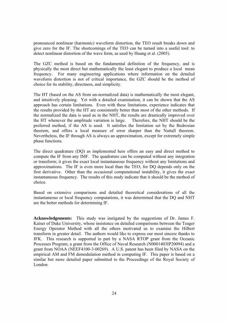
Figure 1.1 Arbitrary sample data used here as an example to illustrate the Empirical AM and FM decomposition through the spline fitted normalization scheme.

31

Figure 1.2 The maxima of the absolute values (red circle) of the data given in Figure 2.1 and the spline fitting (green line) through those values. The spline line is defined as the envelope (instantaneous amplitude) to be used as the base for normalizing the data.

32

Figure 1.3 The one time normalized data (blue line) compared with the original data (red line). Notice that the normalized data still have values greater than unity.

33

Figure 1.4 The data (blue line) and various envelopes: though both envelopes agree in general, the modulus of the AS (green line) shows high frequency intra-wave modulations, while the empirical envelope (red line) fitted by the spline method is smooth.

34

Figure 1.5 IF of the sample data based on various methods: Direct Quadrature (DQ), Hilbert Transform (HT), and Normalized Hilbert Transform (NHT), with the data plotted at 1/10 scale.

35

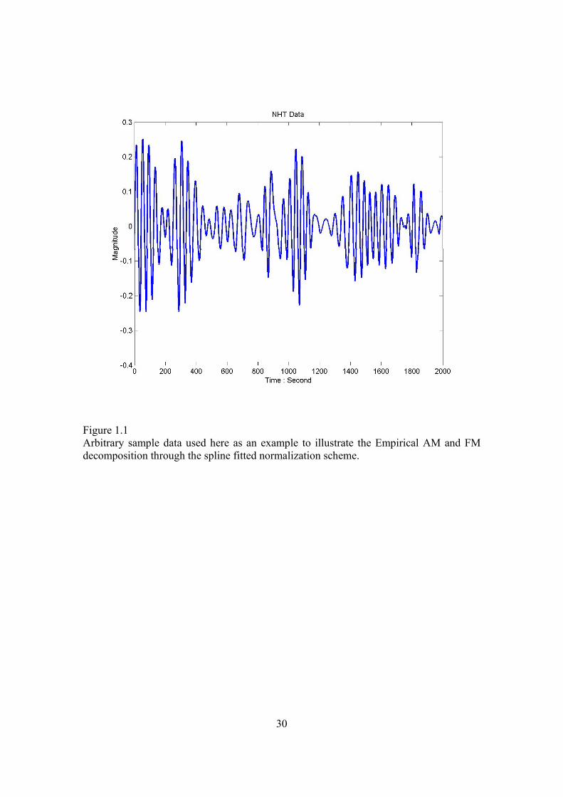
Figure 1.6 The energy based Error Index values for the sample data. Notice the Error Index is high whenever the waveform of the data is highly distorted from the regular sinusoidal form.

36

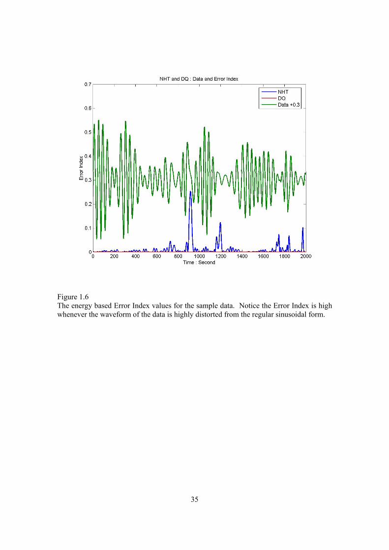
Figure 2.1 The modeled damped chirp Duffing waves based on Equation (38).

37

Figure 2.2 Comparison of the imaginary part from the AS based on a simple Hilbert transform, normalized Hilbert transform, and quadrature. While the quadrature is identical with the theoretical result, the AS’s are visibly different from the theoretical results, especially the one without normalization, where the jump condition at the ends forced the AS to diverge from the data.

38

Figure 2.3 Fourier power spectral density for the normalized carrier (FM, the red line) and envelope (AM the blue line). They are overlapping each other, indicating that the data violated the limitation of the Bedrosian theorem; therefore, the contamination of the FM part defined from the AS by the AM variations is to be expected.

39

Figure 2.4 IF computed from the various methods: Teager Energy Operator (TEO), Generalized Zero-Crossing (GZO), Hilbert Transform (HT), Normalized Hilbert Transform (NHT), Direct Quadrature (DQ), and the theoretical value (Truth). The IF from the HT (without normalization) and the TEO perform poorly.

40

Figure 2.5 Using the ratios of IF values given in Figure 3.6 to the truth as a measure of error directly. Other than at the very beginning, the DQ gives nearly a perfect ratio of one.