BRL-TRW30 , •' l • > pv .

0>

oo oo r- CNJ <

I Q

•.-• v*

TECHNICAL REPORT BRL-TR-3030

BRL TESTS FOR CONSISTENCY OF VULNERABILITY MODELS

DAVID W. WEBB S *4 Ä g I £ > % I W"

•-. uGT «JO lJw3 1 gg AUGUST 1989

>•../•;; 5"':' •« <-«....• /On *'»•'

^-'J 5i3a

APPROVED FOR PUBLIC RELEASE; DISTRIBUTION UNLIMITED.

U.S. ARMY LABORATORY COMMAND

BALLISTIC RESEARCH LABORATORY ABERDEEN PROVING GROUND, MARYLAND

••' N '" "i

JL «-

DESTRUCTION NOTICE

Destroy this report when it is no longer needed. DO NOT return it to the originator.

Additional copies of this report may be obtained from the National Technical Information Service, U.S. Department of Commerce, Springfield, VA 22161.

The findings of this report are not to be construed as an official Department of the Army position, unless so designated by other authorized documents.

The use of trade names or manufacturers' names in this report does not con- stitute indorsement of any ccrrmercial product.

SECURITY CLASSIFICATION OF THIS PAGE

REPORT DOCUMENTATION PAGE Form Approved OMB No. 0704-0188

la. REPORT SECURITY CLASSIFICATION

UNCLASSIFIED lb. RESTRICTIVE MARKINGS

2a. SECURITY CLASSIFICATION AUTHORITY

2b. DECLASSIFICATION/DOWNGRADING SCHEDULE

3. DISTRIBUTION/AVAILABILITY OF REPORT

Approved for public release; distribution unlimited

4. PERFORMING ORGANIZATION REPORT NUMBER(S)

BRL-TR-3030

5. MONITORING ORGANIZATION REPORT NUMBER(S)

6a. NAME OF PERFORMING ORGANIZATION

Ballistic Research Laboratory

6b. OFFICE SYMBOL (If applicable)

SLCBR-SE-P

7a. NAME OF MONITORING ORGANIZATION

Ballistic Research Laboratory 6c ADDRESS {City, State, and ZIP Code)

Aberdeen Proving Ground, MD 21005-5066 7b. ADDRESS (C/ty, State, and ZIP Code)

ATTN: SLCBR-DD-S Aberdeen Proving Ground, MD 21005-5066

8a. NAME OF FUNDING/SPONSORING ORGANIZATION

8b. OFFICE SYMBOL (If applicable)

9. PROCUREMENT INSTRUMENT IDENTIFICATION NUMBER

8c ADDRESS (City, State, and ZIP Code) 10. SOURCE OF FUNDING NUMBERS

PROGRAM ELEMENT NO.

PROJECT NO.

TASK NO.

WORK UNIT ACCESSION NO.

11. TITLE (Include Security Classification)

TESTS FOR CONSISTENCY OF VULNERABILITY MODELS 12. PERSONAL AUTHOR(S)

David W. Webb 13a. TYPE OF REPORT

TR 13b. TIME COVERED

FROM TO 14. DATE OF REPORT (Year, Month, Day) |15. PAGE COUNT

August 1989 16. SUPPLEMENTARY NOTATION

17. COSATI CODES

FIELD

I!

•*

GROUP SUB-GROIJP -^ mode

18, SUBJECT TERMS {Continue, on reverse if necessary and identify by block, number) I consistency^/ffi%'r,£b tfv/A-j- hypothesis testing.

density function f ,J, .'Ayi,, < r power cumulative distribution function -f*ws /rn*,n,~ -j{ ! > ') ft ; yc.J' zh£z

.9. ABSTRACT {Continue on reverse if necessary and identify by block number) , . , Small sample live-fire testing has been recently revived in the US Army's study of armored vehicle vulnerability. A statistically based procedureis proposed to test for consistency between these live-fire results and the predictions of coinputer simulation models. This procedure is compared with other candidate statistical procedures in their ability to reject false simulation based estimates of kill probabilities. S

It

20. DISTRIBUTION/AVAILABILITY OF ABSTRACT

D UNCLASSIFIED/UNLIMITED El SAME AS RPT. • DTIC USERS

21. ABSTRACT SECURITY CLASSIFICATION

22a. NAME O^ RESPONSIBLE INDIVIDUAL David W. Webb

22b. TELEPHONE (Include Area Code) 278-6646

22c. OFFICE SYMBOL SLCBR-SE-P

DD Form 1473, JUN 86 Previous editions are obsolete. SECURITY CLASSIFICATION OF THIS PAGE

ACKNOWLEDGEMENTS

The author wishes to acknowledge Dr. J. Richard Moore, retired from the Ballistic Research Laboratory, for the initial ideas and guidance in the research efforts, and Jerry Tho- mas and William E. Baker, Ballistic Research Laboratory, and Lawrence D. Losie, Vulnerability/Lethality Division, for their detailed look at the report; and Annette Wiseman for preparing the manuscript.

Accession For

"NITS GF'.A£I DTIC TAS 1;::-,:-=:T.---.-.- ,:,-d Ji.~.'-L"l-::>XLon.-

t G

I I;v_

M

:;•.!/'or al

111

TABLE OF CONTENTS

Page

ACKNOWLEDGEMENTS ui

LIST OF ILLUSTRATIONS .vii

I. INTRODUCTION 1

H. TEST CONCEPTS 2

m. PROCEDURE 1- THE ORDER BY PROBABILITY (OP) PROCEDURE 3

IV. PROCEDURE 2 - THE KILLS TEST 3

V. PROCEDURE 3-THE MORE-LIKELY RESPONSE (MLR) TEST 4

VI. PROCEDURE 4 - THE SQUARED DISTANCE MEASURE (SDM) TEST... 5

VH. AN ILLUSTRATIVE EXAMPLE 6

VIE. PROCEDURE COMPARISONS 13

DC THE FISHBOWL ARGUMENT. 13

X FURTHER NOTES AND RECOMMENDATIONS 21

XI. CONCLUSIONS 21

LIST OF SYMBOLS 23

APPENDIX 25

DISTRIBUTION LIST 29

LIST OF ILLUSTRATIONS

Page

1. Hypothetical 5-component example: All possible outcomes and measures of performance 7

2. Hypothetical 5-component example: Summary of Order by Probability (OP) Procedure 8

3. Hypothetical 5-component example: Summary of Kills test 9

4. Hypothetical 5-component example: Summary of More-Likely Response (MLR) test 10

5. Hypothetical 5-component example: Summary of Squared Distance Measure (SDM) test 11

6. Hypothetical 5-component example: Rejection regions for each procedure...« 12

7. Possible power versus power plots 14

8. Power versus power plots for K=6 15

9. Power versus power plots for K= 10. 16

10. Median power of the four candidate procedures 17

11. Sample outcome space with events drawn proportional to density 19

12. All possible 5% rejection regions for sample outcome space 20

vii

I. INTRODUCTION

Since the end of World War II and up until recent years the United States Army has conducted limited live-fire tests of armored fighting vehicles (AFVs) to investigate the interaction occurring between munitions and these vehicles. The live-fire tests were con- ducted only occasionally because of extremely high costs cf resources necessary for those tests. Although vulnerability studies of AFVs have used the insights gathered from such vehi- cle tests, they have relied more on mathematical modeling, computer simulation, live-fire tests of components, and inferences made from firing at armor plate. The live-fire testing of armored vehicles has recently intensified involving a very limited number of vehicles and shots. One question which Army researchers wish to answer is how well do computer model predictions compare with the results from live-fire field testing of AFVs. The answer to that question is the topic of this report.

The outcome of a direct hit on a target vehicle may be examined on three different lev- els. We may look at

1. the entire system (e.g., catastrophic kill),

2. subsystems (e.g., personnel, fire control), and

3. components (e.g., projectile tubes, propellant cases).

If the test results are described as either "kill" or "no-kill", we have a Bernoulli trial in which the outcome can be one of only two possible states. Vulnerability estimates are expressed as kill probabilities (Pk)'s, which represent the proportion of hits resulting in a kill.

Recently a computer model has been developed that incorporates randomness in its cal- culations so that simulated repeated firings at an AFV under identical shot conditions pro- duce varying degrees of destruction. Through many runs of the model, vulnerability research- ers can obtain hypothesized values (or estimates) of the true Pk's for the entire system, sub- systems and components. It would be an experimental luxury to be able to fire munitions at hundreds of AFVs under the same shot conditions to see how well these hypothesized values from the model replicate the live-fire results. Due to the destructive nature of the test and the cost of AFVs, such an experiment is economically infeasible. Usually the same munition or different munition types are fired at vehicles under varying shot conditions with no duplica- tion of shots and the experimenter is left to assess the validity of computer based vulnerability estimates from the firing of a single round. It is impossible to statistically analyze a hypothesized Pk on the basis of one fired round. However, if we look at a group of com- ponents, for example, then we can make a statistically valid statement for the corresponding group of Pk's if we assume that the components are independent. What is meant by indepen- dence is that the outcome of any component (kill or no-kill) has no influence on the probabil- ity that the other components in the group will be killed.

This report details four procedures for testing a group of hypothesized probabilities. The argument is presented that one of the four is the asymptotically most powerful test of the possible procedures. This problem was first studied by Dr. J. Richard Moore, formerly of the US Army Ballistic Research Laboratory (BRL), in response to requests from the Vulnerability/Lethality Division (VLD) of BRL. The author joined Dr. Moore in his research in 1986. Since then VLD has used some of the results in exarnining computed esti- mates, which were calculated with a expected value model, for consistency with observed test results from firings at AFVs.

H. TEST CONCEPTS

Assume that as a result of our computer simulation, we obtain a set of Pk estimates. Perhaps they are for a group of components within a subsystem of the AFV. Denote this set of estimates by the vector [p°, p£, • • •, p/°], where p° is the estimated kill probability of the il

component of interest and / is the number of components. Also, let the true but unknown kill probabilities be denoted by the vector [pi( p2,—, pj. If we assume that the components are independent, then we may begin to develop our test strategy by writing the null hypothesis:

Ho: Pi = Pi°' P2 = P2'•' P/ = P/°-

Note that while this is similar to the hypothesis for the binomial test, one fundamental difference exists: We allow for the p°'s to be unequal. We call this a test of generalized bino- mial proportions. The binomial test is a special case of this, namely p. = p., for all i,j.

If the data do not support the null hypothesis, then it is rejected in favor of its converse, the alternative hypothesis,

HA: pj jfcpj0 for some i.

The alternative hypothesis states that only one inequality has to exist; i.e., only one estimate needs to be incorrect. However, because the analysis is based upon as little as one round, gross inequalities are needed before a procedure will be able to reject the null hypothesis with satisfactory power.

Suppose we observe a set of/ independent Bernoulli outcomes from the live fire testing (denoted by 0 or 1, corresponding to no-kill or kill, respectively), and write them in the form of a row vector A = [a^ a^,..., a,]. For example, if /=5, we may observe A = [0,1,0,0,1]. There are Z possible outcome vectors Alf Aj,..., A^, which we collectively define to be R., Any test of the null hypothesis requires a measure of performance (MOP) for each of the 2* outcomes and some ordering of the measure. At this point we branch our discussion into four different MOP's and thus four different testing procedures.

m. PROCEDURE 1 - THE ORDER BY PROBABILITY (OP) PROCEDURE

This procedure rejects the null hypothesis if the observed vector is among a defined crit- ical set of "rarest" outcomes. The MOP for the procedure is simply P(A), the probability with which outcome A occurs assuming our hypothesized probabilities p°, p£, •», P/. The outcome set, fi, is ordered by P(A) in increasing magnitude, and each outcome is numbered so that A(1) is the least likely outcome and Af2i> is most likely. We then define a cumulative function B, where

B; = Bi-i + P(A(i)) i=2,3,4, ...,2'

We pick a desired level of significance, a, and find "c" such that c = max {]ß- < a and P(A^) -£P(Aß+1))}. Then the set RR = {A(1), A,-,..., A^} represents the c rarest out- comes in H and is the rejection region for the test of HQ at a l00a% level of significance. The "test statistic" is the observed outcome vector A; if A € RRop, then H0 is rejected.

IV. PROCEDURE 2-THE KILLS TEST

This test uses for its MOP, the number of kills (l's) observed. The underlying notion is that under the null hypothesis, a certain number of kills is expected. Letting K(A) denote the number of kills in our observed outcome vector A, then the expected value of K( A) is

E[K(A)]=Pl0 + p2

0 + ... + P;

= E Pi°- i=i

If the observed K(A) is much smaller than E[K(A)], then perhaps the model estimates are inflated estimates of the true kill probabilities. Likewise, if the observed K(A) is much larger than E[K(A)], then the estimated kill probabilities are probably too small.

To perform this test, we begin by calculating K(A) and P(A) for ail 2 outcomes. The outcomes are then ordered in increasing magnitude by K(A) and numbered, so that

K(A(1))<K(A(2))<---<K(A(2<)).

The order among outcomes with equal K(A) is irrelevant. Similar to the OP procedure the "cumulative function" is calculated. Since rejecting H0 may be due to either too small or too large a value of K(A), a two-tailed test is used. Critical values ct and c2 are selected so that the actual alpha level

PpCCA^cJ + PtKCA)^]

is maximized but still less than or equal to a. The rejection region for this test is RRK = {A|K(A) G {0,1, • • • cj u {c2,C2+l, • • • /}}. The model estimates will be rejected as inconsistent with the field tests if A G RRK.

V. PROCEDURE 3 - THE MORE-LIKELY RESPONSE (MLR) TEST

This test examines the number of more-likely, or "correct" responses where a more- likely response is defined as

1i

1 if aj = 0 when p? < .5, or if a} = 1 when p? > .5

5 if p° = .5

^0 otherwise

In other words a more-likelv response is the response which we expect to see more often than not in the long run. So if p{ = .8 we would expect to observe a kill more often than a no-kill. If aj = 1, a kill, then 7. = 1 and the observed response is considered "correct". When p.° = .5, we are essentially saying that we have no inclination as to which response is more likely. Therefore we compromise and always assign ^ = .5.

The MOP is the total number of correct responses

M(A) = 7i + 72 + • * • +7/

i=l

The reasoning behind this procedure is that if we observe an unusually low number of more-likely responses, then our model estimates are too large when they should be smaller and/or too small when they should be larger. We also note that it is possible to observe too many correct responses. This would tend to indicate that our large estimates (p° > .5) are not large enough and/or that our small estimates (p? < .5) are not small enough.

The expected value of M( A) is

E[M(A)] = ML + S*/2 + My

where

ML = E(

1-P/

>) foraUp°<.5

j

Mu=EPj° foraUP;>.5 j

* O S = number of Pj equal to .5

We start by calculating M(A) and P(A) for all possible outcomes. The outcomes are arranged in increasing magnitude by M(A) without regard for ties so that

MCA^MC^O-SMCA^)

The cumulative function is computed as usual. Since obtaining a value of M(A) much smaller or larger than the expected value leads us to believe that HQ is false, a two-tailed test is desired. Critical values c1 and <^ are selected as in the Kills test to maximize the actual alpha level. The rejection region becomes RRMLR

= {A|M(A) e {0,1, • • • cj U {c2, c2 + 1, • • • /} }, and we will reject H0 at the a level of significance if Ae RR^LR- In practice, though, c2 will usually not exist and a one-tailed test will be used instead.

VI. PROCEDURE 4 - THE SQUARED DISTANCE MEASURE (SDM) TEST

This test involves the calculation of a "squared distance measure" for each component of the outcome vector. The SDM is (p{° - af) . Squaring assures that all values are positive so that each component produces an additive effect; it also increases the "penalty" for responses which are very far from p?. Note that the SDM for any given component must lie in the interval [0,1]; and the two values SDM may take on are more extreme the nearer to 0 or 1 p° is. The SDM acts as a penalty functioa As p° approaches 0 (or 1), the penalty associated with being incorrect is greater. If p° is close to .5 (i.e., we have less confidence in our ability to predict aj), then the penalty for an incorrect response is not much different than the SDM for a correct response. The MOP is simply the sum of the SDM's,

S(A) = (p1°-a1)2 + (p2

0-a2)2+ ••• + (p,°-a,)2

= £(Pi°-ai)2

i=l

The expected value of S( A) is

E[S(A)] = J) Pi° (1 - Pi°) i=l

Again, we calculate S(A) and P(A) for each of the Z outcomes, and arrange them in decreas- ing magnitude by S(A) with no regard for ties so that

S(A(1))>S(A(2))>--->S(A(2())

The Bj's are computed in the usual fashion. We would tend to believe that H0 is false if S(A) is too large, therefore a one-tailed procedure is used. Given alpha, we select c which satisfies

c = maxtilB^aandSCA^) ^(A^)}.

The set of outcomes RRS = {A|S(A) > S(A,c))} represents the rejection region for our test of H0. Therefore if S(A) > S(A,c)) we reject H0 at the a level of significance.

Vn. AN ILLUSTRATIVE EXAMPLE

Assume that the model estimates of kill probabilities for five independent tank com- ponents are as follows:

A = [.23, .64, .19, .91, .70]

Figure 1 shows each of the 2 = 32 possible vector outcomes along with their associated P(Aj), K(Aj), M(Aj), and S(Aj). The outcomes are ordered by a binary counting scheme. The OP procedure is illustrated in Figure 2. Note that the vectors are now ordered by their probability of occurrence. The rejection region for an a = .05 level of significance is all the outcomes above the line. Figure 3 shows the Kills test ordering scheme and resultant two- tailed rejection region outside the two lines. Note the additional columns PfK^A^)] and B[K(Afiv)]. Since our test statistic is K(A), vectors having an equal number of kills are indis- tinguishable. Therefore P[K(A,jO] represents the probability of getting K(A^) kills and B[K(A,Ö)] represents the cumulative probability for the same number of kills. In Figure 4, the MLR test is shown. Although a two-tailed procedure can be used, the rejection region only includes a lower tail of six vectors. This is because the vector with M(A,32)) = 5 has a probability mass greater than alpha. The columns P[M(A~)] and B[M(A,jO] are analogous to the additional columns of Figure 3. We see the SDM test in Figure 5. It has a rejection region of 13 vectors containing the largest values of S(A,.x). Note that B14 < a, however A,14)

is not in the rejection region. This is because S(A.14)) = S(A,15J and B15 > a. Recall that in each of the tests, outcomes with equal MOP's are considered indistinguishable. If we had allowed A,14) € RRS and A,15) £ RRS then we would be violating the rule by differentiating between two outcomes with the same SDM. Figure 6 summarizes the rejection regions of the four procedures, with OP having the largest region and the kills test having the smallest.

The hypothesized probabilities are: [0.23,0.64, 0.19,0.91,0.70]

Vector Prob. Kills MLR SDM

\ P(Ai) K(Aj) M(Ai) S(Aj)

00000 0.00606 0 2 1.8167 00001 0.01415 1 3 1.4167 00010 0.06130 1 3 0.9967 00011 0.14303 2 4 0.5967 00100 0.00142 1 1 2.4367 00101 0.00332 2 2 2.0367 00110 0.01438 2 2 1.6167 00111 0.03355 3 3 1.2167 01000 0.01078 1 3 1.5367 01001 0.02515 \-':i'- 4 1.1367, 01010 0.10897 2 4 0.7167 01011 0.25427 3 5 0.3167 01100 0.00253 2 2 2.1567 01101 0.00590 3 3 1.7567 01110 0.02556 3 3 1.3367 01111 0.05964 4 4 0.9367 10000 0.00181 1 1 2.3567 10001 0.00423/ 2 2 1.9567 10010 0.01831 2 2 1.5367 10011 0.04272 3 3 1.1367 10100 0.00042 2 0 2.9767 10101 ,0.00099 3 1 2.5767 10110 0.00429 3 1 2.1567 10111 0.01002 4 2 1.7567 11000 0.00322 2 2 2.0767 11001 0.00751 3 3 1.6767 11010 0.03255 3 3 1.2567 11011 0.07595 4 4 0.8567 11100 0.00076 3 1 2.6967 11101 0.00176 4 2 2.2967 11110 0.00764 4 2 1.8767 11111 0,01782 5 3 1.4767

Figure 1. Hypothetical 5-component example: All possible outcomes and measures of performance.

The hypothesized probabilities are: [0.23,0.64,0.19,0.91,0.70]

Vector Prob. Cum.Prob. i

% P(V Bi

1 10100 0.00042 0.00042 2 11100 0.00076 0.00118 3 10101 0.00099 0.00217 4 00100 0.00142 0.00359 5 11101 0.00176 G.00536 6 10000 0.00181 0.00717 7 01100 0.00253 0.00969 8 11000 0.00322 0.01291 9 00101 0.00332 0.01623

10 10001 0.00423 0.02046 11 10110 0.00429 0.02475 12 01101 0.00590 0.03065 13 00000 0.00606 0.03671 14 11001 0.00751 0.04422 15 11110 0.00764 0.05186 16 10111 0.01002 0.06188 17 01000 0.01078 0.07266 18 00001 0.01415 0.08680 19 00110 0.01438 0.10118 20 11111 0.01782 0.11900 21 10010 0.01831 0.13731 22 01001 0.02515 0.16246 23 OHIO 0.02556 0.18802 24 11010 0.03255 0.22057 25 00111 0.03355 0.25412 26 10011 0.04272 0.29684 27 01111 0.05964 0.35648 28 00010 0.06130 0.41778 29 11011 0.07595 0.49373 30 01010 0.10897 0.60270 31 00011 0.14303 0.74573 32 01011 0.25427 1.00000

Figure 2. Hypothetical 5-component example: Summary of Order by Probability (OP) Procedure.

The hypothesized probabilities are: [0.23,0.64, 0.19,0.91,0.70]

Vector Kills Probability Cumulative Probability i

% K(A(i)) n%) PtKCA^)] Bi BtKCA^)]

1 00000 0 0.00606 0.00606 0.00606 0.00606 2 00001 0.01415 j 0.02021) 3 00010 0.06130/ 0.08151 4 00100 0.00142) 0.08945 0.08293) 0.09552 5 01000 0.010781 0.09371 6 10000 0.00181/ 0.09552 ] 7 00011 2 0.14303 \ 0.23855 i 8 00101 2 0.00332 0.24186 9 00110 2 0.01438 0.25624

10 01001 2 0.02515 I 0.28139 11 12

01010 01100

2 2

0.10897 1 0.00253 j > 0.32355

0.39036 1 039289 ) 0.41906

13 10001 2 0.00423 0.39711 14 10010 2 0.01831 | 0.41542 15 10100 2 0.00O42 | 0.41585 16 11000 2 0.00322 / 0.41906 17 00111 3 0.03355 \ 0.45262 18 01011 3 0.25427 0.70689 19 01101 3 0.00590 0.71278 20 OHIO 3 0.02556 0.73835 21 10011 3 0.04272 \ > 0.40811 0.78107 \ 0.82717 22 10101 3 0.00099 0.78206 23 10110 3 0.00429 0.78635 24 11001 3 0.00751 0.79387 25 11010 3 0.03255

0.00076/ 0.82642

26 11100 3 0.82717, 27 01111 4 0.05964) 0.88682 28 10111 4 0.01002 0.89684 29 11011 4 0.07595 0.15501 0.97279 0.98218 30 11101 4 0.00176 \ 0.97455 31 11110 4 0.00764/ 0.98218 32 11111 5 0.01782 0.01782 1.00000 1.00000

Figure 3. Hypothetical 5-component example: Summary of Kills test.

The hypothesized probabilities. are: [0.23,0.64,0.19,0.91,0.70]

Vector MLR Probability Cumulative Probability i *o M(A(i)) rev PIMCAQ)] Bi BIMCAgp]

1 10100 0 0.00042 0.00042 0.00042 0.00042 2 00100 1 0.00142 0.00185 3 10000 1 0.00181 0.00366 4 10101 1 0.00099 > 0.00927 0.00465 0.00970 5 10110 •4

i 0.00429 0.00894 6 11100 1 0.00076 0.00970 7 00000 2 0.006061 0.01576' 8 00101 2 0.00332 0.01908 9 00110 2 0.01438 0.03346

10 01100 2 0.002531 0.03599, 11 10001 2 0.004231 } 0.07146 0.04021' • 0.08116 12 10010 2 0.01831 j 0.05852 13 10111 2 0.010021 0.06854 14 11000 2 0.00322 0.07176 15 11101 2 0.00176 0.07352 16 11110 2 0.00764 0.081161 17 00001 3 0.014151 0.095301 18 00010 3 0.06130 0.15660 19 00111 3 0.03355 0.19015j 20 01000 3 0.010781 0.20093 21 22

01101 OHIO

3 3

0.00590' 0.02556 j I 0.25183

0.20683 J 0.232391

• 0.33299

23 10011 3 0.04272 0.27511! 24 11001 3 0.00751 0.28262' 25 11010 3 0.03255 0.31517 26 11111 3 0.01782 0.33299 J 27 00011 4 0.14303 0.47602

0.50117 28 01001 4 0.02515 29 01010 4 0.10897 0.41274 0.61014 0.74573 30 01111 4 0.05964 0.66978 31 11011 4 0.07595, 0.74573] 32 01011 5 0.25427 0.25427 1.00000 1.00000

Figure 4. Hypothetical 5-component example: Summary of More-Likely Response (MLR) test.

10

The hypothesized probabilities are: [0.23,0.64,0.19,0.91, 0.70]

i Vector

%

SDM Probability Cumulative Bi

Probability BßCAß)]

1 10100 2.9767 0.00042 0.00042 0.00042 0.00042 2 11100 2.6967 0.00076 0.00076 0.00118 0.00118 3 10101 2.5767 0.00099 0.00099 0.00217 0.00217 4 00100 2.4367 0.00142 0.00142 0.00359 0.00359 5 10000 2.3567 0.00181 0.00181 0.00540 0.00540 6 11101 2.2967 0.00176 0.00176 0.00716 0.00717 7 8

01100 10110

2.1567 2.1567

0.00253 0.00429

> 0.00682 0.00969) 0.01399 j

0.01399

9 11000 2.0767 0.00322 0.00322 0.01721 0.01721 10 00101 2.0367 0.00332 0.00332 0.02053 0.02053 11 10001 1.9567 0.00423 0.00423 0.02475 0.02475 12 11110 1.8767 0.00764 0.00764 0.03239 0.03239 13 00000 1.8167 0.00606 0.00606 0.03845 0.03845 14 15

01101 10111

1.7567 1.7567

0.00590 0.01002

0.01592 0.044351 0.05437 j

0.05437

16 11001 1.6767 0.00751 0.00751 0.06188 0.06188 17 00110 1.6167 0.01438 0.01438 0.07626 0.07626 18 19

01000 10010

1.5367 1.5367

0.01078 0.01831 0.02909

0.087041 0.10535 j

0.10535

20 11111 1.4767 0.01782 0.01782 0.12316 0.12316 21 00001 1.4167 0.01415 0.01415 0.13731 0.13731 22 OHIO 13367 0.02556 0.02556 0.16287 0.16287 23 11010 1.2567 0.03255 0.03255 0.19542 0.19542 24 00111 1.2167 0.03355 0.03355 0.22897 0.22897 25 26

01001 10011

1.1367 1.1367

0.02515 0.04272

[ 0.07287 0.25412) 0.29684 j

0.29684

27 00010 0.9967 0.06130 0.06130 0.35814 0.35814 28 01111 0.9367 0.05964 0.05964 0.41778 0.41778 29 11011 0.8567 0.07595 0.07595 0.49373 0.49373 30 01010 0.7167 0.10897 0.10897 0.60270 0.60270 31 00011 0.5967 0.14303 0.14303 0.74573 0.74573 32 01011 0.3167 0.25427 0.25427 1.00000 1.00000

Figure 5. Hypothetical 5-component example: Summary of Squared Distance Measure (SDM) test.

11

Order by Probability (OP) Procedure -- RR OP (14 outcomes)

10100 11100 10101 00100 11101 10000 01100 11000 00101 10001 10110 01101 00000 11001

Kills Test -- RR K (2 outcomes)

00000 11111

More-likely Response (MLR) Test ~ RR MLO (6 outcomes)

10100 00100 10000 10101 10110 11100

Squared Distance Measure (SDM) Test - RR SDM (13 outcomes)

10100 11100 10101 00100 10000 11101 01100 10110 11000 00101 10001 11110 00000

Figure 6. Hypothetical 5-component example: Rejection regions for each procedure.

12

VIII. PROCEDURE COMPARISONS

To study the four procedures, 2000 pairs of /-dimensional probability vectors were ran- domly generated for / = 5, 6, 7, 8, 9, and 10. The first vector of a pair (h0 hA) was considered the hypothesized probability vector and the second was considered the alternative probability vector. The level of significance was set at a = .05. The power of each test (i.e., the proba- bility of rejecting H0 when HA is true) was computed for each pair (h0, hA).

Figure 7 shows a graphic way of comparing the power of two test procedures, call them A and B. For a given pair of vectors (h0,1TA), we compute the ordered pair (ßA, /?B) where ßA and /?B are the powers of A and B respectively. Then the scatterplot of all 2000 points, (ßA, ßB), will give us a comparison of the two tests. If Procedure A is more powerful than Procedure B, then we expect to see a graph similar to Figure 7(A). If the opposite is true, the plot will be similar to Figure 7(B). But if both procedures have approximately the same power, then Figure 7(C) is the proper scatterplot.

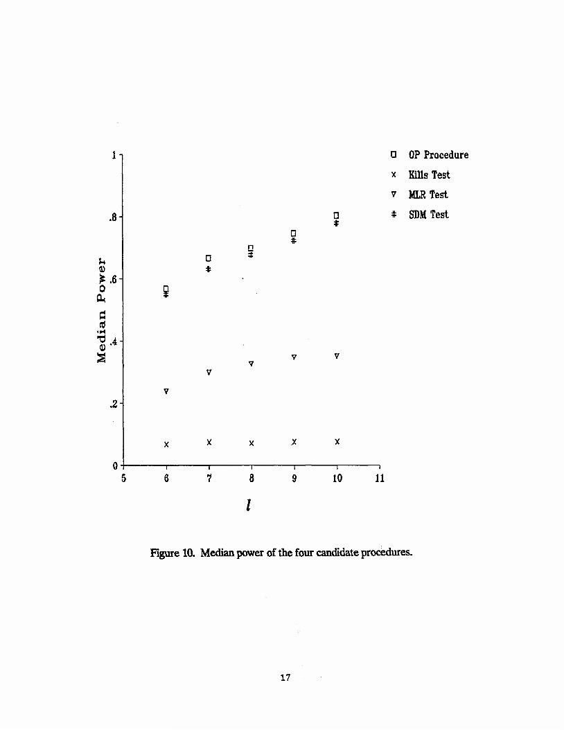
Comparisons of the four procedures consistently show the OP procedure to be the most powerful (See Figures 8 and 9). The SDM test appears to be only slightly less powerful. The MLR and Kills tests both showed poor ability to reject H0 when other Ps were used.

These findings are reinforced when the median power of each procedure is computed. In Figure 10, we see again that OP slightly outpowers SDM, with MLR and Kills exhibiting less power. It is impossible to tell for certain which of the four procedures is best unless we know "hA. But from the strictest viewpoint in which we assume no prior knowledge of the Pj's, this is not the case. When we do not know any information about hA, we must assume that all possible TTA's are equally likely. Therefore it makes sense to pick that procedure with the greatest number of outcomes in its rejection region.

IX. THE FISHBOWL ARGUMENT

Assume that the null hypothesis we are interested in testing is one that completely defines the distribution of the outcome space fi. For example, our illustrative example from Figures 1-6 is concerned with the null hypothesis

H0: Pl = .23, p2 = .64, p3 = .19, p4 = .91, p5 = .70.

Given the estimated probabilities in this hypothesis, P(Aj) can be calculated for all possible outcomes. Another null hypothesis that we may be interested in is:

H0: pj = .23, p2 = .64, p3 = .19, p4 = p5

Note that this does not contain all the probability estimates needed to compute P(A), how- ever it is certainly a valid hypothesis. We will define a simple null hypothesis to be one that completely defines the distribution of the outcome space, and denote it by HQ.

13

TEST fl POWER

00

l r k

. :"ä: ".'!•' .••*•• •'.v.-.'-V. '"-•?•'

TEST ft POWER

CO

Figure 7. Possible power versus power plots.

14

II

Ul at •=> a Ul o o a a. a. o

4 u- * o • ••-.. ..t

4~'.*...V«Sv~-

v4

iS3i anw JO a3i«iod

II

: •..*• £;£.~-i

•' • "•: •'i.'ii

Ui 3 o

^

II

•^Äv,:

. '•. '. •'W.;:-' •' •.

.'.**!;'•'.•.'. .'•

/.^iV-->' •. ' ••?v-" .- • -...'• X;«...

2J. 1S3J. MIS JO 33fl0d

vt>

o «ts efl <-J

O Ul Q: 7 3 a Ul o J •-

o a ct U- Ü. co •X a

«> u. •t. o

1 ,j

Ul 3 6 o CL;

«i <U

1S31 STIIX JO «PlOd

15

•ft

II

^^-y'.-^rV.-:•.;•.;:./:. ; •:.'-. >"•." ,.' \". *:. \ . -' •.

' v"^'!>••! v'y''-r^,' ?i ," . •' '" •"• ••.•""' * "•""" '; * _'.'•_

: • . z1 ".''*• *%^'^'• *•,"!' • •;•*•;!•• ••:' ,•• " ;'.*•*•*'"*' " •*"• " :| ,_.' V - """' ' • ** .. • i.*!1" "!•••*••** .* »*"."••:•"•>' •' "•.!.":'• ".""*"•"*"•'*'*• ""•:. * • * ~. ••• •

. _ * i*"' */..v.*" w"•••"•• .";• .*••".' *: •""• '-'""v": • *. '•'" :"•• '*.

• . "• • L •. ••• •

•"••* .'• . ";*••. * " ' .* '•"• "* .";. ••;. '•.-C'/."'--

" . * * * " '" .***". '-**.:*' - ". «* •••.;•*'• •{•• ':'•'••. . •• r! **' *': ""• *'•

> ."'"*" •• • •t •'.*,*•' •••* ".-"

.*•"-• V " . .". • -0 '*•* . - * .'»• ' - ' ''

•: .• : :•' '".•• ••;" •!." * '!•••"-. %r.' '•

• " . • » "."•."" . * *" '•'>'.ii ,*

. <*

JLS31 *nw JO a3nod

II

• •;;:'.,'j'0^Si- •'' ••-..v'Tv-"-.-;?^

.-• •.~£.1-;T*S

"•:i.'--"y>iSr-'

1-1

II

'•;*£/•••

ul O ex

U

o iü o LU a. a. o

en 3 t/3 h.

o ?> ?• Uc

Id <u 3 * a o a. PL,

E

ct

a UJ u o O.

CL O

u. o

Ui 3 O 0.

iS3i was JO aanod

lS3i snu JO ÜJ3BQ<i

16

.8

u CD M 0

ö cd

«H •d ©

.2-

8

0 OP Procedure

x Kills Test

v MLR Test

a *

# SDM Test

D n *

D *

*

-1 1 1 1 1 1

6 7 8 9 10 11

Figure 10. Median power of the four candidate procedures.

17

Now make the additional assumption that an experiment has a finite outcome space, n. If we are interested in testing some simple null hypothesis at the a level of significance, how many different ways can we perform a test of H^ and which is the optimal way?

To attempt to answer these questions let ft be of size N, m < N, and {Oj, 02, • • • Om} be any subset of ft such that under H^,

P(01) + P(02)+ ••• +P(Om)<a.

Then we claim that {Ov 02, • • • Om} is a rejection region for some test of HQ. Why? Because under HQ, the chance of observing an outcome from this subset is less than or equal to alpha, our desired level of significance. Therefore we have the foundations of a statistical test, even if the reasoning behind the selection of the subset is not specified.

To help explain this concept, Figure 11 shows an example of an outcome set with N=16. Each circle represents one of the 16 possible outcomes and its size is proportional to the den- sity of the outcome under the simple null hypothesis. In Figure 12, each group of circles (out- comes) connected by a horizontal line symbolizes a subset satisfying our condition (i.e., a < .05) to be a rejection region for some test of the simple null hypothesis. The probability of observing an outcome from each subset is indicated by the number in the right column. Note that these values (which are computed by summing the probabilities of the outcomes in the subset) are all less than or equal to .05, the desired alpha level, and that the addition of any other outcome to each set makes the new sum greater than .05. We therefore consider each of these 24 subsets a rejection region to test HQ.

For each rejection region, the probability of observing an outcome in that region is at most a under the simple null hypothesis. However, if some alternative hypothesis is true, the probability of observing an outcome in the rejection region (thereby correctly rejecting HQ) is some other value 1-ß, which we call the power of the test. Unfortunately the power is unk- nown to us if we do not know which alternative hypothesis is true. At best, we can only say that all alternative hypotheses are equally likely. Therefore each outcome in a rejection region is equally likely to occur, and the optimal rejection region is that one which contains the most outcomes. The way to build this rejection region is to include the least likely out- comes until no more can be added. In Figure 12, the star labels the rejection region that we would use since it contains six outcomes, more than any other rejection region.

As an analogy, assume you are given a small fishbowl partially filled with water and a large number of pebbles with which to completely fill it. Also assume that each pebble has a different volume. If you were instructed to raise the water level to the top of the fishbowl by adding as many pebbles as possible, how would you set out to do so? Instead of occupying space with one large pebble, you would fill the same space with smaller pebbles. Therefore you would begin by selecting the smallest pebble and putting it in the bowl. Then you would drop in the second smallest pebble. The third pebble would be the next smallest, and so on untü the water level reaches the brim. The remaining pebbles would of course be the largest ones.

18

© .HAS

© .011

.188

© .oos

0 .016

O 0 .ose #047

.127

© .006

O • OSS

11

.048

0 .010

O .091

.071

.624 .884

OUTCOME SET

Figure 11. Sample outcome space with events drawn proportional to density.

19

—o 0

o-o-o O-O

o o-o

—o-

O OO

o-o-O-O —o o—O-O- o-o

o—O o o—O-O

O

o o-o-o-O-O—O -o-o-o o-o-O—

o-o— o o-o-O- o-o

o <>

O

o-O-O —o-o

•o-O-O o

O

O

o

o

o

o o o Ü

o

u 15

U

ALPHA .050 .050 .049 .048 .050 .048 .049 .043 .050 .050 .047 .049 .050 .050 .049 . .048 ft .050 .043 .049 .046 .050 .048 = 047 .049

CU <o CO o CO CU ,_ cu c^ 00 o o o ^- *— ^- cu CO 0) *• •* o o o o o o o o o o o

—

*

Figure 12. All possible 5% rejection regions for sample outcome space.

20

The OP procedure uses this "fishbowl" technique by filling up the rejection region with those outcomes having the smallest probabilities. The only restriction to the technique is that the last outcome entered into the rejection region cannot have the same density as any out- come excluded from the region

X. FURTHER NOTES AND RECOMMENDATIONS

The OP procedure was only tested for 1 = 5,6, 7, 8, 9 and 10, for two reasons. Firstly, the data that spawned this research was only for small /, namely / < 10. Secondly, the compu- tational time and storage needed to compute the P(A)'s, B's, etc. grows nearly exponentially with each unit increase in /. Simulations using / = 12 were attempted but ran non-stop for a couple of days on a Gould 9050 minicomputer. *

Since the SDM tests does a good job of mimicking the OP procedure it may be an easier test to use when / is larger than 10, if the distribution of S(A) can be approximated. Initial attempts to find such an approximation were not successful. A listing of the computer pro- gram is given in the Appendix at the end of this report.

XL CONCLUSIONS

This problem is complicated by the fact that we must judge the entire set of computer generated estimates on a single shot. It must be admitted that while OP is the best procedure of those studied, occasionally H0 was not rejected although the alternative hypothesis differed greatly from it Great care must be taken in interpreting the final decisioa In rejecting H0

we can confidently say that the set of hypothesized kill probabilities is incorrect. However, venturing to say which components are incorrect and by how much is dangerous. It is vital to remember that we are trying to make inferences from one round. If we do not reject H0, then this does not allow us to "accept H0 as being true". It simply says that there is not enough evidence to say that H0 is false. We cannot validate the estimates, we can only state that they are consistent with the live fire results.

We must take care to see that our assumption of independent components is met. All the calculations involved in the OP procedure are made under these assumptions. Therefore the selection of components is critical, and we should avoid including incendiary components, shielded components, etc., in the analysis.

The OP procedure works best of the four tried because it does not lose any information by collapsing the data into a univariate test statistic. It simply creates that rejection region with the most outcomes.

* Lawrence D. Losie of the Ballistic Research Laboratory has made recommendations for improving the computational efficiency of the OP procedure. This work is unpublished but may be obtained through private communication with Mr. Losie.

21

TABLE OF SYMBOLS

A

A?V ai

B[K(A(i))]

B[M(A0)] B[S(AJ

Bi PA C c,

E

hA

\ K K(A) / M(A) MLR MOP ML

Mu

Oi OP P(A) P[K(A )] P[M(A )] P[S(A(ij]

Pk

Pi RR * S SDM S(A) n

vector of observed outcomes •th

.th

i ordered vector of observed outcomes armored fighting vehicle il component of vector A level of significance probability of observing that number of kills (or less) associated with the i1' ordered vector A,^ probability of observing that MLR value (or less) associated with the i' ordered vector Am

probability of obsrving that SDM value (or less) associated with the i' ordered vector A(j)

cumulative function value of vector A,f) power of some test procedure A critical value for one-sided rejection region lower critical value for two-sided rejection region upper critical value for two-sided rejection region more likely response value for i component of vector A expected value operator alternative hypothesis vectors of alternative probabilities null hypothesis vector of hypothesized probabilities null hypothesis which completely defines the distribution of the outcome space number of kills in vector A number of components number of "more-likely-responses" in vector A more-likely-response measure-of-performance expected number of non-kills for the group of components whose estimated probability of kill is less than one-half expected number of kills for the group of components whose estimated probability of kill is greater than one-half an element of the outcome space fi order-by-probability probability of vector A probability of observing that number of kills associated with the il ordered vector A(i)

probability of observing that MLR value associated with the il ordered vector A(i)

probability of observing that SDM value associated with the i ordered vector A,^ probability of kill true probability of kill for il component estimated probability of kill for i component rejection region number of estimated probabilities equal to one-half squared-distance-measure squared-distance-measure for vector A set of all possible outcomes

23

APPENDIX

25

APPENDIX

c FILE; vul.f c c This program takes a vector of k probabilities of 0,1 outcomes, c enumerates all possible outcome vectors and calculates the c probability of each, using the vector of outcome probabilities c given. It then sorts each of the outcome vectors according to c their probability of occurence. It calculates and prints the c cumulative probability. c c k < 13, is the dimension of the vector. c p(i), i=l,k is the vector of input probabilities. c jout(i,j) is the 2**k by k matrix of possible outcome vectors. c c This program is written to run in the interactive mode but c it can be run batch mode by reading k, the desired alpha level c and p(i), i=l,k from one file and writing the results in c another file. For example, vul.e < data.inp > data.out will c read input from a file named data.inp and write the results c into a file called data.out. c

common jout(4097,10),prob(4097),n,k double precision prob(4097),cum(4097) dimension p(12) read(5,*) k read(5,*) dalp read(5,*)(p(i) ,i = l ,k) epsilon=0.00000001 n=2**k

c GENERATE MATRIX OF ALL POSSIBLE OUTCOMES do 10 j=l,n do 10 i=l,k jout(j,i)=0

10 continue do 20 i=l,k ni=2**(k-i) nj =2*ni do 20 nk=ni+l,n,nj do 20 nl=nk,nk+ni-l

j out(nl,i) = 1 20 continue

«rite(6,120) write(6,130)(p(i),i=l,k) write(6,140) write(6,150) do 30 i = l,n prob(i) = 1. do 30 j = l,k prob(i) = prob(i)*p(j)**(jout(i,j))*(1.-p(j))**(1-jout(i,j))

30 continue

27

ORDER ALL OUTCOMES BY PROBABILITY, FROM LOWEST TO HIGHEST do 50 j=l,n-l do 50 m=j + 1,n if (prob(j ).gt.prob Cm)) then do 40 i=l,k isave = j out(j ,i) j out(j ,i)=jout(m,i) jout(m,i)=isave

40 continue save=prob( j ) prob(j)=prob(m) prob(m)= save endif

50 continue CALCULATE CUMULATIVE DISTRIBUTION FUNCTION

cum(1)=prob(1) do 60 j=2,n cum( j)=cum(j-1)+prob(j)

60 continue do 70 i=l,n write(6,160)i,prob(i),cum(i),(jout(i,j),j=l,k)

70 continue • DETERMINE REJECTION REGION

irr=n 80 irr=irr-l

if (cum(irr).ge.dalp) goto 80 if (prob(irr+1)-prob(irr).It.epsilon) goto 80 talp=cum(irr)

: OUTPUT REJECTION REGION VECTORS write(6,170)irr do 110 i=1,irr write(6,180)(jout(i,j), j = l ,k^

110 continue write(6,190)talp

120 format('The input probabilities are:') 130 format(12f6.3) 140 format(//' Vector Prob. Cum.Prob. Vector') 150 formate No. '/) 160 format(i6,2x,el0.5,f10.6,2x,lli2) 170 format(/'The rejection region consists of these ',i3,' vectors:'/) 180 format(4x,lli2) 190 format(/'The true alpha level is ',f6.3)

stop end

28

No of Copies Organization

(Undue, unlimited) 12 Administrator (Unclass., Umlud) 2 Defense Technical Info Center (Classified) 2 ATTN: DTICDDA

Cameron Station Alexandria, VA 22304-6145

No of Copies

1

HQDA (SARD-TR) WASH, DC 20310-0001

Commander US Army Materiel Command ATTN: AMCDRA-ST 5001 Eisenhower Avenue Alexandria, VA 22333-0001

Commander US Army Laboratory Command ATTN: AMSLC-DL Adelphi, MD 20783-1145

Commander Armament RD&E Center US Army AMCCOM ATTN: SMCAR-MSI Picatinny Arsenal, NJ 07806-5000

Commander Armament RD&E Center US Army AMCCOM ATTN: SMCAR-TDC Picatinny Arsenal, NJ 07806-5000

Director Benet Weapons Laboratory Armament RD&E Center US Army AMCCOM ATTN: SMCAR-LCB-TL Watervliet, NY 12189-4050

Commander US Army Armament, Munitions

and Chemical Command ATTN: SMCAR-ESP-L Rock Island, IL 61299-5000

Commander US Army Aviation Systems Command ATTN: AMSAV-DACL 4300 Goodfellow Blvd. St Louis, MO 63120-1798

Director US Army Aviation Research

and Technology Activity Ames Research Center Moffett Field. CA 94035-1099

(Ctan. coir) 1

(Didw. caly) 1

(Clm. only)

1

Organization

Commander US Army Missile Command ATTN: AMSMI-RD-CS-R (DOC) Redstone Arsenal, AL 35898-5010

Commander US Army Tank Automotive Command ATTN: AMSTA-TSL (Technical Library) Warren, MI 48397-5000

Director US Army TRADOC Analysis Command ATTN: ATAA-SL White Sands Missile Range, NM 88002-5502

Commandant US Army Infantry School ATTN: ATSH-CD (Security Mgr.) Fort Benning, GA 31905-5660

Commandant US Army Infantry School ATTN: ATSH-CD-CSO-OR Fort Benning, GA 31905-5660

The Rand Corporation P.O. Box 2138 Santa Monica, CA 90401-2138

Air Force Armament Laboratory ATTN: AFATL/DLODL Eglin AFB, FL 32542-5000

Aberdeen Proving Ground Dir. USAMSAA

ATTN: AMXSY-D AMXSY-MP, H. Cohen

Cdr, USATECOM ATTN: AMSTE-TO-F

Cdr, CRDEC, AMCCOM ATTN: SMCCR-RSP-A

SMCCR-MU SMCCR-MSI

29

AUTHOR'S DISTRIBUTION LIST

No. of No. of Copies Organization Copies Organization

Dir, USAMSAA ATTN: AMXSY-R, A.W. Benton

AMXSY-R, Bobby Bennett AMXSY-R, Harold Pasini AMXSY-R, Walter Mowchan AMXSY-G, Wilbert J. Brooks

Dir, USACSTA ATTN: STECS-MA-A, Vernon Visnaw

Commander US Army Development &

Employment Agency ATTN: MODE-TED-SAB Fort Lewis, WA 98433

AFWL/SUL Kirtland AFB, NM 87117

Aberdeen Proving Ground

Cdr, USATECOM ATTN: AMSTE-TO-F

AMSTE-EV-S, Larry West

30

USER EVALUATION SHEET/CHANGE OF ADDRESS

This laboratory undertakes a continuing effort to Improve the quality of the reports it publishes. Your comments/answers below will aid us in our efforts.

1. Does this report satisfy a need? (Comment on purpose, related project, or other area of interest for which the report will be used.)

2. How, specifically, is the report being used? (Information source, design data, procedure, source of ideas, etc.)

3. Has the information in this report led to any quantitative savings as far as man-hours or dollars saved, operating costs avoided, or efficiencies achieved, etc? If so, please elaborate.

4. General Comments. What do you think should be changed to improve future reports? (Indicate changes to organization, technical content, format, etc.)

BRL Report Number Division Symbol

Check here if desire to be removed from distribution list.

Check here for address change.

Current address: Organization Address

-FOLD AND TAPE CLOSED-

Director U.S. Army Ballistic Research Laboratory AT'.CN: SLCBR-DD-T (NEI) .Aberdeen Proving Ground, MD 21005-5066

OFFICIAL BUSINESS

BUSINESS REPLY LABEL FIRST ClASS PERMIT NO. 13063 WASHINGTON D. C.

POSTAGE WILL BE PAID BY DEPARTMENT OF THE ARMY

NO POSTAGE NECESSARY IF MAILED

IN THE UNITED STATES

Director U.S. Army Ballistic Research Laboratory ATTN: SLCBR-DD-T(NEI) Aberdeen Proving Ground, MD 21005-9989