The submitted m a n u a r m has been authored by a contractor of the U. S. Government under contract No. W-31-104ENG-38. Accordingly. the U. S Government retam a nonexclutiw. royalfy-fraa licenrs to plMirh or reproduce the published form of this contribution. or allow others to do so. for

I U. S. Gowrnmant DU-.

Decay Rates of Various Bottomonium systems*

SNUTP-95-089

ANL-HEP-CP-95-65

0 S..T I 1

Seyong I i i m t High Energy Physics Division, Argonne National Laboratory, 9700 South C a s .Avenue, Xrgonne. IL 60.139. USA

r-.;ing the Bodwin-Braaten-Lepage factorization theorem in heavy quarkonium decay and production processes. we calculated matrix elements associated with S- and P-wave bottomonium decays via lattice QCD simdation methods. In this u-ork, we report preliminary results on the operator matching between the lattice expression and the continuum expression at one loop level. Phenomenological implications are discussed using these preliminary .US matrix elements. -

Heavy quarkonium decay rates can be written as a sum of factorized products of perturbative coefficients and non-perturbative matrix elements Ell.

r (H -+ LH) =

for the decays intn light hadrons and

r(H -+ EM) =

for the electromagnetic decays, where A is a fac- torization scale and fn's are the coefficients from four-fermi vertices.

For t.he case of bottomonium decays, we have calculat-ed the lattice regulated matrix elements in th i s factorization theorem[2], using the leading order non-relativistic QCD lagrangian

(3)

The matrix elements in which we are interested are :

(4) 'Work supported by the U.S.Department of Energy, Divi- sion of High Energy Physics, Contract W-31-109-ENG- 38. \Vork done in collaboration with D.K.Sinclair and G . T. Bodwin 'current address : Center for Theoretical Physics, Seoul National University. Seou1,Korea

(5)

Hs = ( 1 PI $tT=XXtT" II, 11 P ) / M 2 . f7)

To make use of lattice regulated matrix ele- ments (which we have calculated already in [Z]) for phenomenology, we need to perform operator "renormalization" which translates lattice - regu- lated matrix elements into continuum M S matrix elements,

j

where 0 ' s are ordered following the velocity scal- ing law [3]. Once we calculate the matrix Zij , we obtain OF by inverting the Z matrix :

(9) j

From GI, FI, HI, and Ha, we note that neces- sary 0 ' s are :

I = *txx'*,

for the S-wave case and

for P-wave. Here, we dicuss our preliminary res- ults on the renormalization of these operators (full details will be reported elsewhere [4]).

Firstly, we derive Feynman rules for our lat- tice lagrangian upto O(g2) from the Iattice quark propagator,

G(2.t + 1) = (1 - H0/2n)~U~(Z,t)(l- Ho/2n)"G(Zlt) + 6,-.ij&+l,O, (14)

with G(Z,t) = 0 for t < 0 and Ho = -A2/2Mo - Estrb (A is lattice covariant derivative, ESub = 3(1 - ~ g ) / - W o , uo = (Ol#TrUp~aqlO)f,n = 2). Then, using these Feynman rules, we calculate one loop renormalization of the operators, (10) -

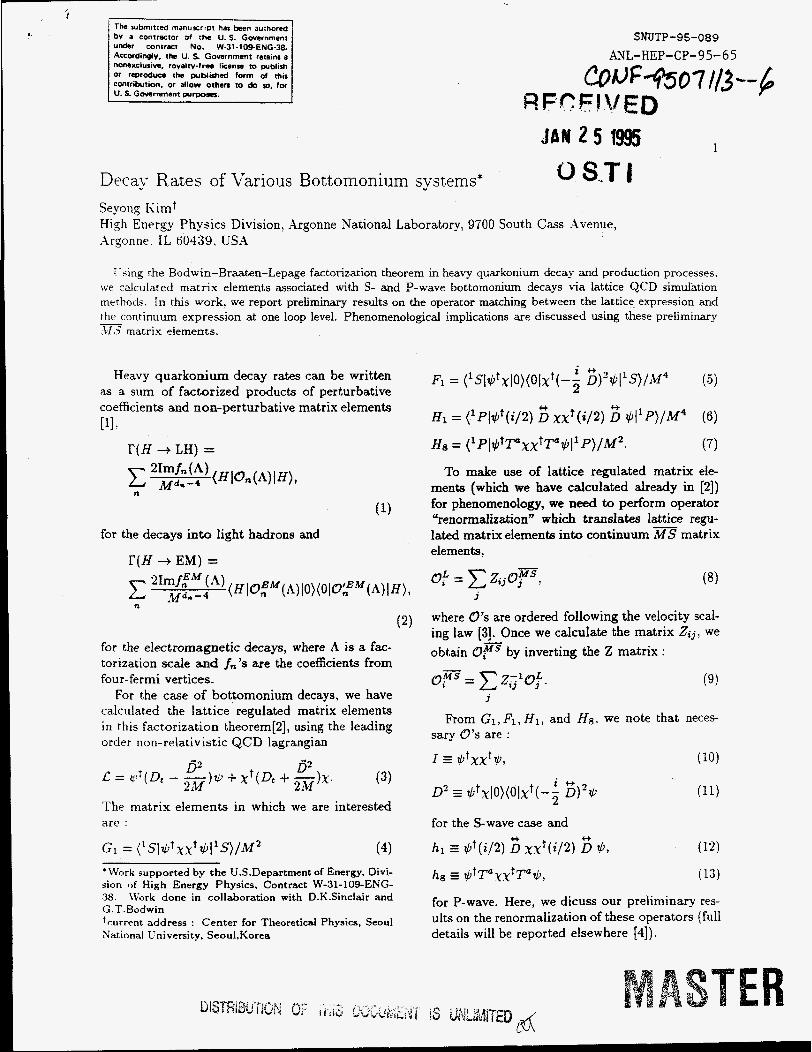
Necessary Feynman diagrams for the part of D2 which contributes to the mixing with the con- tinuum operator I are given in Fig 1. A dotted line means the temporal component of the gluon field and a wavy line means the spatial component of gluon field (in the following figures, we use the same convention). a) has the lattice V2 vertex, b) has the g ' p vertex, and c) is the tadpole con- tribution. Af'ter finding analytic expressions for these diagrams, we take $(external momentum) + O(except the tadpole contribution) to pick out pieces for the continuum I.

(13).

Figure 1. Feynman diagram for the power diver- gent part of D2 renormalization.

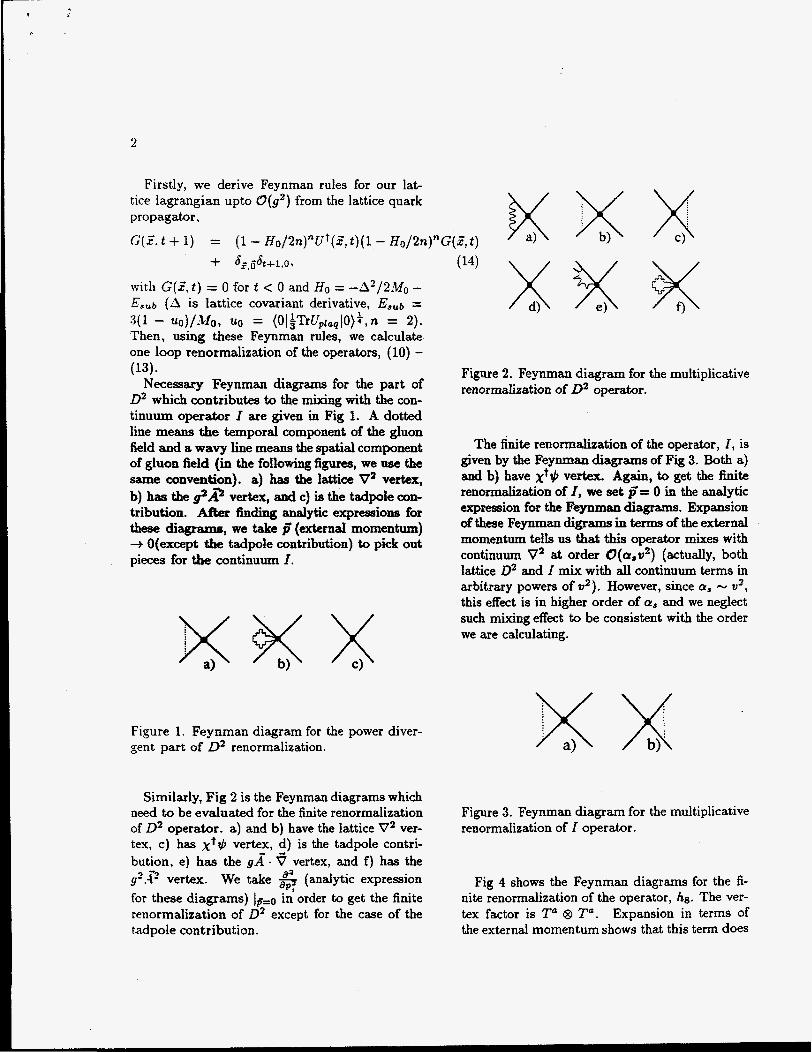
Similarly, Fig 2 is the Feynman diagrams which need to be evaluated for the finite renormalization of D2 operator. a) and b) have the lattice V2 ver- tex, c) has xty5 vertex, d) is the tadpole contri- bution, e) has the g x . ? vertex, and f ) has the g2;i? vertex. We take 4 (analytic expression

ap, for these diagrams) in order to get the finite renormalization of D2 except for the case of the tadpole contribution.

Figure 2. Feynman diagram for the multiplicative renormalization of Da oprator.

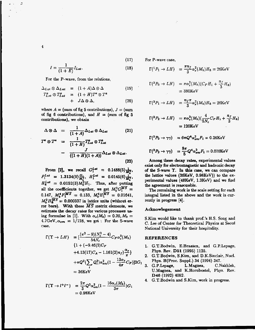
The finite renormalization of the operator, I, is given by the Feynman diagrams of Fig 3. Both a) and b) have xt$ vertex. Again, to get the fhite renormalization of I, we set p" 0 in the andytic expression for the Peymnan diagrams. Expansion of these Feynman digrams in terms of the external momentum tells us that this operator mixes with continuum V2 at order O(a,u2) (actually, both lattice D2 and I mix with all continuum terms in arbitrary powers of v2) . However, since os - w2, this effect is in higher order of a, and we neglect such mixing effect to be consistent with the order we are calculating.

Figure 3. Feynman diagram for the multiplicative renormalization of I operator.

Fig 4 shows the Feynman diagrams for the fi- nite renormalization of the operator, hs. The ver- tex factor is Tc @ Tu. Expansion in terms of the external momentum shows that this term does

3

Table 1 numerical values of Feynman integrals

Figure 4. renormalization of hs

Feynman diagrams the multiplicative

Figure 5. Feynmau diagrams for the multiplicat- ive renormalization of irl

not mix with hl- With p’= 0, we obtain the fi- nite renormalization contribution from these dia- grams.

With p’= j’ = 0, the Feynman diagrams in Fig 5 gives the contribution to the finite renormaliz- ation of the operabr, 31. The vertex factor is lattice version of e V.

Figure 6. Feynman diagrams for the mixing con- tribution from hl to hs

Finally, Fig 6 shows the Feynman diagrams for the mixing of the operator, h l , with he. The ver- tex factor is the same as Fig 5. With zero external

diagram fig la fig l b fig I C

fig 2a fig 2b fig 2c fig 2d fig 2e fig 2f fig 3

fig 4af4b fig 5af5b

fig 6a+6b+6c+6d (fig 6a+6b+6c+6d) log

Vega output 0.4781( 8) 0.7008( 2)

0.12476(3)

0.005360(4) 0.1411(100)

-O.8448( 100)

-0.18774( 3)

-0.27241 (5) -0.116804(7)

-0.001346(3) -0.11773(3)

-0.0060293(9)

0.010717(2)

0.0013

momentum, these diagrams have a logarithmic in- frared divergence. Therefore, these digrams need extra care. We subtract logarithmic divergent piece from the analytic expression of these dia- grams if Cip? 5 I? when the integral is evalu- ated numerically. The last entry in Table 1 is the difference between the logarithmically divergent piece which we use in the subtraction and that for the MS expression.

After we get the analytic expression for the Feynman diagrams we listed in the above, we eval- uate the integrals numerically by use of VEGAS. Table 1 is the summary of the numerical values of each Feynman integral. We used a, = 0.135 and Mb = 1.71 in lattice units. Note that 1%

in the integral differs from that in the simulation (1.5) because the tadpole improvement scheme we employed tells us that Mb = Mo/uo.

For the S-wave, from the relations,

Diat = (1 + G)D2 + FI ILat = (1 + E)I,

(15) (16)

where G = (sum of fig 2 contributions), F = (sum of fig 2 contributions), and E = (sum of fig 3 contribution), we get

4

1 (1+ E) '= ILot -

For the P-wave, from the relations,

Atat @ ALur = (1 + A)& @ A (19)

+ J A @ A , (20) T f a t 8 T,b,, = (1 + H)T' 8 T"

where A = (sum of fig 5 contributions), J = (sum of fig 6 contributions), and H = (sum of fig 5 contributions), we obtain

Ator 8 At&. J -

((1 + WI1+ 4) (22)

From [2], we recdi Gf"' = 0.1488(5)*, Ffot = 1.3134(9)-&, HfO' = 0.0145(6)4

Af. ' Hkat = O.O152(3)M,2Hr. Thus, after putting all the coefficients together, we get M 2 G F = 0.147, M 2 F F = 0.133, M t H F = 0.01641, M t H p = 0.000337 in lattice units (without er- ror bars). With these MS matrix elements, we estimate the decay rates for various processes us- ing fOl?nUk! [I]. with a,(&) = 0.20,Mb = 4.7GeV,ae, = 1/128, we get : For the S-wave case,

-

= 36KeV

I'(3P' + 77) = 67rQ4azmF1 = 0.26KeV

8 r 5 r(sP2 + ~ y ) = -@atmF~ = 0.070KeV

Among these decay rates, experimental values exist only for dectromagnetic and hadronic decay of the Swave T. In this case, we can compare the lattice values (36KeV, 0.98KeV)) to the ex- perimental values (48KeV, 1.3KeV) and we find the agreement is reasonable.

The remaining work is the scale setting for each integral listed in the above and the work is cur- rently in progress [4].

Acknowlegement

S.Kim would like to thank prof.'s H.S. Song and C. Lee of Center for Theoretical Physics at Seoul National University for their hospitality.

REFERENCES

1. G.T.Bodwin, E.Braaten, and G.P.Lepage, (1 + (-9.46(2)C~ ~-

+4.13(17)C~ - l.l61(2)nj)%)

+.Q2(C GMm(l - -$CF)J~GI

Phys. Rev. D51 (1995) 1125. k 2. G.T.Bodwin, S.Kim, and D.K .Sinclair, .Nucl.

Phys. B(Proc. Suppl.) 34 (1994) 347.

U.Magnea, and K.Hornboste1, Phys. Rev. D46 (1992) 4052.

4. G.T.Bodwin and S.Kim, work in progress.

13a I 3. G.P.Lepage, L.Magnea, C.NakhIeh,

= 0.98KeV

DISCLAIMER

This report was prepared as an account of work sponsored by an agency of the United States Government. Neither the United States Government nor any agency thereof, nor any of their employees, makes any warranty, express or implied, or assumes any legal liability or responsibiiity for the accuracy, completeness, or use- fulness of any information, apparatus, product, or process disclosed, or represents that its use would not infringe privately owned rights. Reference herein to any spe- cific commercial product, process, or service by trade name, trademark, manufac: turer, or otherwise does not necessarily constitute or imply its endorsement, recorn- mendation, or favoring by the United States Government or any agency thereof. The views and opinions of authors expressed herein do not necessarily state or reflect those of the United States Government or any agency thereof.