frederik.orellana.dkfrederik.orellana.dk/wp-content/files/diss.pdf · zusammenfassung die...
TRANSCRIPT

MesonicFinal State Interactions
Dissertation
zur Erlangung der naturwissenschaftlichen
Doktorwürde (Dr. sc. nat.)
vorgelegt der
Mathematisch-naturwissenschaftlichen Fakultät
der Universität Zürich
von
Frederik Orellana
aus Dänemark
Begutachtet von
Prof. Dr. Daniel Wyler
Dr. Gilberto Colangelo
Zürich 2002

Die vorliegende Arbeit wurde von der Mathematisch-naturwissenschaftlichen Fakultät derUniversität Zürich auf Antrag von Prof. Dr. Daniel Wyler und Prof. Dr. Ben Moore als Disser-tation angenommen.

A mi abuela : Christina Orellana
A mi tía : Consuelo Orellana

Zusammenfassung
Die vorliegende Arbeit beschäftigt sich mit zwei unterschiedlichen aber verwandten Pro-blemen: 1) Die Grössenordnung der Korrekturen infolge von Endzustandswechselwirkungenin mesonischen Prozessen. 2) Die Frage, wie weit es möglich ist, die Berechnung solcher Kor-rekturen zu automatisieren.
Insbesondere wird untersucht, ob die Diskrepanz zwischen theoretischen und experimentel-len Werten von¶¢/¶ durch die Berüchsichtigung mesonischer Endzustandswechselwirkungenim Zerfall K® ΠΠ erklärt werden kann. Für die präzise Auswertung solcher Korrekturen wur-de ein konsistenter Rahmen entwickelt. Das Ergebnis ist ein System von Integralgleichungen,das mit zwei Konstanten als Eingabe iterativ gelöst werden kann. Von diesen zwei Konstantenkann die eine bestimmt werden durch das Soft-Pion Theorem, die andere ist nicht bekannt. Esfolgt, dass im Moment die Unsicherheit bei der Auswertung von Endzustandswechselwirkun-gen zu gross ist, um eine definitive Aussage zu machen,aberdass das sich ändern wird, sobalddie zweite Konstante bekannt ist. Eine Ward-Identität wurde hergeleitet, welche die Berech-nung der Konstante in der Gittertheorie erleichtern sollte. Die vollständige Berechnung desZerfalls K® ΠΠ in chiraler Störungstheorie ist durchgeführt worden. Sie ist von begrenztemdirekten Nutzen wegen der vielen unbekannten Konstanten, hat aber während der Berechnungder Endzustandwechselwirkungen als Leitfaden gedient.
Für das durchgeführte Studium von K® ΠΠ sind die niederenergetischen Phasen derΠΠ-Streuung wichtig. Ein Kapitel ist der Berechnung elektromagnetischer Korrekturen zu diesenPhasen in chiraler Störungstheorie gewidmet. Die Ergebnisse werden für dasDIRAC Expe-riment wichtig sein, sobald die angekündigte Messung der 2P-2S Energiedifferenz in Pioni-um Ergebnisse liefert. Die Berechnung dient auch als Test der entwickelten Computerberech-nungsprogramme.
Diese Programme werden im letzten Kapitel beschrieben und sind in der ganzen Arbeit ver-wendet worden. In diesen Kapiteln werden auch viele analytische Berechnungen der chiralerStörungstheorie beschrieben und mit der Literatur verglichen.
Das Studium der Verletzung derCP-Symmetrie und der Parameter¶¢ und ¶ sowie dasStudium des Vakuums und des Mechanismus spontaner chiraler Symmetrieverletzung, diesich in der Streuung von Pionen aneinander manifestiert, sind Teil der laufenden Verifika-tion/Falsifikation und Erforschung des elektroschwachen Standardmodels und der Quanten-chromodynamik.
i

Summary
In the present work, two distinct but interrelated subjects are investigated: 1) The importanceof corrections due to final state interactions in mesonic processes. 2) The question of how farit is possible to automatize the calculation of such corrections.
In particular it is explored whether or not the discrepancy of theoretical predictions withexperimental values of¶¢/¶ can be explained by the inclusion of mesonic final state interactionsin the amplitude of the decay K® ΠΠ. A framework has been developed for the precisionevaluation of these corrections in a consistent way. The outcome is a set of integral equationsthat can be solved iteratively, requiring as input two constants of which one is known fromthe soft pion theorem and the other largely unknown. This is at present all that can be done.The conclusion is that the uncertainties involved in the evaluation of final state interactionsare too large for the method to be of any use at presentbut that this will change as soonas the second constant becomes known. A Ward identity is given which should facilitatethe lattice evaluation of the constant. The full calculation of K® ΠΠ in Chiral PerturbationTheory (although of limited direct use, due to the abundance of unknown constants) served asa guideline when calculating the final state interactions.
For the study of K® ΠΠ presented, the low energyΠ+Π- ® Π+Π- phases are crucial, and achapter has been devoted to the study of the inclusion of electromagnetic corrections to theseusing Chiral Perturbation Theory. The results will be relevant for theDIRAC experiment dueto the planned measuring of the energy difference between the 2P-2S levels of pionium. Thecalculation also provides checks of the calculational software developed.
The computational tools developed, are presented in the last chapter and are used through-out. Many calculations in Chiral Perturbation Theory, that have been worked out and checkedwith the literature, are described.
The study of the violation ofCP-symmetry and the parameters¶¢ and¶ as well as the studyof the structure of the vacuum and the mechanism of spontaneous chiral symmetry breakingas revealed by the scattering of pions, are part of the ongoing verification/falsification andexploration of the electro-weak Standard Model and Quantum Chromo-Dynamics.
ii

Contents
Zusammenfassung. . . . . . . . . . . . . . . . . . . . . . . . . . . . . . . . . . . iSummary . . . . . . . . . . . . . . . . . . . . . . . . . . . . . . . . . . . . . . . iiContents. . . . . . . . . . . . . . . . . . . . . . . . . . . . . . . . . . . . . . . . iii
1 Introduction 1
2 Chiral Perturbation Theory 52.1 Introduction. . . . . . . . . . . . . . . . . . . . . . . . . . . . . . . . . . . 52.2 Effective lagrangians. . . . . . . . . . . . . . . . . . . . . . . . . . . . . . 72.3 The Euler-Heisenberg lagrangian for photon-photon scattering. . . . . . . . 72.4 Chiral Goldstone bosons. . . . . . . . . . . . . . . . . . . . . . . . . . . . 92.5 Chiral mesonic lagrangians. . . . . . . . . . . . . . . . . . . . . . . . . . . 102.6 Pion-pion scattering. . . . . . . . . . . . . . . . . . . . . . . . . . . . . . . 14
3 Charged pion-pion scattering 173.1 Introduction. . . . . . . . . . . . . . . . . . . . . . . . . . . . . . . . . . . 173.2 Virtual photons . . . . . . . . . . . . . . . . . . . . . . . . . . . . . . . . . 173.3 Isospin breaking. . . . . . . . . . . . . . . . . . . . . . . . . . . . . . . . . 183.4 Divergent one-loop generating functional. . . . . . . . . . . . . . . . . . . 193.5 One-loop amplitudes. . . . . . . . . . . . . . . . . . . . . . . . . . . . . . 22
4 Final state interactions in non-leptonic kaon decays 254.1 Introduction. . . . . . . . . . . . . . . . . . . . . . . . . . . . . . . . . . . 254.2 Kaon phenomenology andFSI . . . . . . . . . . . . . . . . . . . . . . . . . 264.3 Off-shell matrix elements inCHPT . . . . . . . . . . . . . . . . . . . . . . . 294.4 Dispersion theory. . . . . . . . . . . . . . . . . . . . . . . . . . . . . . . . 334.5 The Omnès method. . . . . . . . . . . . . . . . . . . . . . . . . . . . . . . 384.6 The soft pion theorem for non-leptonic kaon decays. . . . . . . . . . . . . . 434.7 Crossed channel dispersion equations. . . . . . . . . . . . . . . . . . . . . 46
iii

4.8 Solving the equations. . . . . . . . . . . . . . . . . . . . . . . . . . . . . . 504.9 Results and discussion. . . . . . . . . . . . . . . . . . . . . . . . . . . . . 53
5 Computerized quantum field theory 555.1 Introduction. . . . . . . . . . . . . . . . . . . . . . . . . . . . . . . . . . . 555.2 Working with quantum fields. . . . . . . . . . . . . . . . . . . . . . . . . . 595.3 Lagrangians and Feynman rules. . . . . . . . . . . . . . . . . . . . . . . . 645.4 Feynman rules and Feynman diagrams. . . . . . . . . . . . . . . . . . . . . 68
Conclusion 75
A PHI reference manual 77A.1 Installing and loading the packages. . . . . . . . . . . . . . . . . . . . . . . 77A.2 Framework . . . . . . . . . . . . . . . . . . . . . . . . . . . . . . . . . . . 78A.3 Building blocks, lagrangians. . . . . . . . . . . . . . . . . . . . . . . . . . 80A.4 Feynman rules, loops and power counting. . . . . . . . . . . . . . . . . . . 87
B PHI applications 95B.1 QED . . . . . . . . . . . . . . . . . . . . . . . . . . . . . . . . . . . . . . . 95B.2 CHPT, pions . . . . . . . . . . . . . . . . . . . . . . . . . . . . . . . . . . . 96B.3 CHPT, pions and photons. . . . . . . . . . . . . . . . . . . . . . . . . . . . 98B.4 CHPT, mesons. . . . . . . . . . . . . . . . . . . . . . . . . . . . . . . . . . 98B.5 CHPT, pions and virtual photons. . . . . . . . . . . . . . . . . . . . . . . . 100B.6 WeakCHPT . . . . . . . . . . . . . . . . . . . . . . . . . . . . . . . . . . .102
C One-loop amplitudes 105C.1 Pion-pion scattering. . . . . . . . . . . . . . . . . . . . . . . . . . . . . . .105C.2 Non-leptonic kaon decays. . . . . . . . . . . . . . . . . . . . . . . . . . . . 109C.3 Decomposition of the kaon decay amplitude. . . . . . . . . . . . . . . . . . 121C.4 Loop functions . . . . . . . . . . . . . . . . . . . . . . . . . . . . . . . . .128
Bibliography 131
Acknowledgements 145
Curriculum Vitae 146
iv

Chapter 1
Introduction
The dynamics of quarks, which are regarded as the bulk constituents of matter on earth, be-comes untractable or irrelevant in the low energy world which is dominated by the stronginteraction. This world is described in terms of particles called hadrons, which are thoughtto be bound states of quarks, and, in contrast to quarks, directly observable. The mostabundant hadrons in nature are the ground states of the possible two- and three-quark en-sembles of the lightest two quark flavors: The proton, the neutron and the positive, nega-tive and neutral pion. With more quark flavors, other particles can be formed. In the lowenergy regime one restricts to the lightest two or three flavors, and thus to the light pseu-doscalar triplet or octet (pions, kaons and the eta-meson) and their interactions, that is, thestrong, electromagnetic (EM) and weak interactions. The low energy description and in-terplay of these forces is subtle: They are all governed by the symmetries underlying theelectro-weak Standard Model [Gla61, Wei67a, Sal68] (SM) and Quantum Chromo-Dynamics[GW73a, GW74, GW73b, Pol73] (QCD), but for instance, whereas the weak and strong in-teractions of mesons are described solely in terms of the contact interactions of the mesonsallowed by the symmetries, theEM interaction is additionally described by including the ex-change of photons. The reason for the feasibility of this is that the weak gauge bosons areheavy, the strong interaction is a short-range force, but the photon is light and electromag-netism is a long-range force. The tool for the description of these particles and forces iseffective field theory and in particular the effective field theory known as Chiral PerturbationTheory [GL84, GL85] (CHPT). When comparing with experimental data, other supplemen-tary tools become useful, namely dispersion relations exploiting the analytic properties of theamplitudes.
1

2 CHAPTER 1. INTRODUCTION
Symmetries of the Standard Model
The symmetries governing low energy phenomena are the fundamental symmetries of natureas well as the symmetries imposed by theSM. That is: The amplitudes have to satisfy Lorentzinvariance, analyticity, unitarity and crossing symmetry, as well as approximate chiral SU(N)´ SU(N) flavor symmetry spontaneously broken down to vectorial symmetry and explicitlybroken by small mass terms. Moreover the strong and electromagnetic lagrangians satisfycharge-parity (CP) invariance, whereas the weak lagrangian hasCP violating terms. What willbe explored is whether these unbroken and broken symmetries and their effective lagrangiansgive a realistic description of the material world as seen by experiment. The symmetry issuesunder consideration here are:
• Verification of the mechanism of approximate chiral symmetry - size of the quark con-densate.
• Determination of the size of the directCP symmetry breaking parameter¶¢/¶.
• Determination of the size of isospin symmetry breaking.
Low energy data
The amplitudes calculated in the present work are for the following processes: KS ® Π0Π
0,Π±Π±® Π
±Π±, ΓΓ ® ΠΠ (ΓΠ ® ΓΠ). The two last amplitudes are not directly accessible to
experiment, but can be extracted from other processes as indicated in the listing below of themost recent relevant experiments:
KS® Π0Π
0
• CERN NA-31 [NA3, B+88, B+93], K® Π0Π
0.
• CERN NA-48 [NA4, F+99], K® Π0Π
0.
• Fermilab E-731 [E73, G+93], K® Π0Π
0.
• KTEV E-832 [E83, AH+99], K® Π0Π
0.
Π±Π±® Π
±Π±
• Brookhaven E-865[E86, P+01], K l4 decays.
Notice that theCERN DIRAC [DIR, Sch00, Lan] experiment could in principle also give highprecision data for the last amplitude if they would in a next generation measure transitionenergies.

3
Calculational ingredients
The primary theoretical ingredient is the perturbative expansion of amplitudes using the chirallagrangians and straight-forward Feynman diagram analysis. The working out of Feynmandiagrams and amplitudes is a tedious and error prone undertaking. Therefore, as much as pos-sible has been done in an automatized fashion. Indeed, one major motivation for the presentwork was to see how far one can push the envelope w.r.t. computerizingCHPT. The authorhas developed a computer program christened "PHI " for this purpose. The program drawson previous work of others [MBD91a, KEM92, Mera, WMSBa, Hah01]; the new part beingthe addition of the capability of dealing with effective theories. The programming languageused isMathematica [Wol00]. Also, a general feature of this whole thesis is that non-trivialcalculations are provided explicitly in form ofMathematica notebooks [Ore]. As mentionedabove, the amplitudes calculated will be unitarized or improved by means of dispersion rela-tions. Other ways of saying this are that final state interactions shall be included or that pion(or meson) rescattering shall be accounted for. Two technical ways of doing this are common:The Omnès method and the inverse amplitude method. Here, the first of these shall be used.
Structure of the thesis
The chapters fall in two main categories:
1) The first three chapters and the last appendix, which deal with low energy formalism, thatis, CHPTand dispersion relations: In chapter,2 the strongCHPT formalism is briefly described.In chapter3, this is extended to include electromagnetism. Chapter4 contains a discussion ofmesonic final state interactions in Ks ® 2Π0. The amplitude is worked out usingCHPT to oneloop and dispersion relations to sum the final-state (unitarity) diagrams to all orders. AppendixC contains formulae too large to be displayed in the main text.
2) Chapter5 and appendicesA andB, which deal with computerization ofCHPT and fieldtheory in general as implemented in the calculational packageFeynCalc and extended by theauthor with the packagePHI: In chapter5, basic concepts of quantum field theory are intro-duced in a computerized fashion, that is, aMathematica syntax for these is defined, someof the computational tools developed are described and some examples are worked out. Ap-pendixA is a reference manual toPHI. AppendixB contains short descriptions of calculationscarried out withPHI. These include the calculations used in chapter3 and chapter4, as well ascalculations of results already avaliable in the literature. These last calculations serve as testsof the program. They all agree with results available in the literature. The actual calculationsare available in form ofMathematica notebooks that can be downloaded from theFeynCalc

4 CHAPTER 1. INTRODUCTION
web-site.
Typography
For abbreviationsSMALL CAPS are used.Bold typewriter tekst is used forMathemat-ica code. Italic small caps are used for names ofMathematica packages. Filenames arequoted. Excerpts fromMathematica notebooks are indicated with a beginning and an endinghorizontal line.

Chapter 2
Chiral Perturbation Theory
In this chapter the framework is set up in which the calculations of the subsequent chapterswill be made. This includes a brief introduction to effective lagrangians andCHPT as wellas a discussion of some of the main features ofCHPT. Towards the end of the chapter afew examples of using computer algebra techniques in calculations are given; the reader isencouraged to consult the notebooks of appendixB containing the full calculations.
2.1 Introduction
According to Weinberg [Wei96], in the early sixties, among quantum field theorists there wasa prevailing sense of crisis. Things seemed to be going nowhere in attempting to describethe newly found weak and strong interactions beyond leading order perturbations. One con-sequence of this was the development of dispersion relation methods (see section4.4) intoan attempt at describing amplitudes completely disregarding the underlying fields using in-stead postulated properties of amplitudes like analyticity, crossing and unitarity. Another con-sequence was the development of current algebra which was also an attempt at calculatingamplitudes without dealing with fields, but instead dealing with currents and postulating analgebra for these. Ironically the basic postulates of these two directions, although claimed tobe "fundamental", were both inspired by leading order perturbative quantum field theory.
At this time, low energyΠΠ scattering was important as a simple process to test the predic-tions for the strong interaction. One unique feature of this process is that it displays completecrossing symmetry. Dispersion theorists tried hard [CM60] to use this to device a self consis-tent system of integral equations, which, assuming the existence of the rho resonance shouldbe able to reproduce the full low energy amplitude - the so-called bootstrap method. Unfor-tunately this method failed - the rho resonance did not even reappear in the crossed channels
5

6 CHAPTER 2. CHIRAL PERTURBATION THEORY
(see section4.4). This should not be seen as a falsification of dispersion relation theory, ratherof one or more of the assumptions involved in the bootstrap method, which all seem plausiblebut which are not exact and the errors of which it is difficult to estimate. These assumptionsinvolve neglecting high energy inelasticity, inclusion of only the rho exchange singularities,and that the rho is predominantly aΠΠ resonance. Current algebra was able to provide a rea-sonable description, but it was equivalent to using a phenomenological lagrangian to leadingorder and there was no way of calculating higher order corrections. This phenomenologicallagrangian was derived in 1967 by Weinberg [Wei67b] by requiring that it be the most generallagrangian respecting Lorentz andCP invariance and chiral symmetry.
As is well known, for the weak interactions ’t Hooft, Weinberg and others came to therescue, introducing the Standard Model and reviving quantum field theory and perturbationtheory. For the strong interactions,QCD was then developed. Low energyΠΠ scattering andother hadronic processes however, were orphaned by these models: In the low energy regime,the blowing up of the strong coupling and confinement makes it impossible to describe exper-iment using perturbation in the coupling constant and quark degrees of freedom.
Instead, the method already endeavoured by Weinberg in 1967 was expanded by Gasser andLeutwyler into a phenomenological framework fully consistent withQCD, or, in fact, derivablefrom QCD (and Lorentz andCP invariance) via the external field method and the equivalencetheorem. The result wasCHPT, which is a low energy theory applying a dual expansion in thequark masses and the external momenta. At each order a new phenomenological lagrangiancomes into play.
The shortcoming ofCHPT is that the 0,1 and 2-loop calculations available are only validat very low energies (. 1GeV) and higher order calculations are senseless because of thehuge number of phenomenological parameters in the higher order lagrangians. Examinationof a method for extending the domain of validity by other means is the subject of chapter4. This method involves using dispersion relations in combination withCHPT. The successof this reflects the fact mentioned that although dispersion theory failed miserably with therho-bootstrap, what was to blame was not the method itself nor the underlying symmetries,but rather the additional assumptions made. Thus, crossing and analyticity remain (by gen-eral consensus) perfectly good, exact assumptions and can be applied as additional pieces ofinformation to supplement or test theCHPT predictions. Elastic unitarity is only approximate,but the application of it has more predictive potential. The remainder of this chapter is anintroduction to effective lagrangians andCHPT.

2.2. EFFECTIVE LAGRANGIANS 7
2.2 Effective lagrangians
Nowadays effective lagrangians are widely used in particle physics phenomenology when amore fundamental theory is either unknown or unsuited for calculating the quantity one is inter-ested in. Typically, heavy degrees of freedom are integrated out in order to achieve lagrangianscontaining only the light particles, taking advantage of the fact that large-scale dynamics islargely unaffected by very short distance structures and interactions. The effects from heavyparticles are then parameterized by coupling constants which have to be determined from ex-periment or using some model. Amplitudes are renormalized "order by order" in the energyexpansion, each order having a lagrangian with contact interactions to absorb loop infinitiesfrom lower order lagrangians. That is, effective theories are not necessarily renormalizable inthe traditional sense. Examples include the Euler-Heisenberg theory of photons forE � me
[HE36], the Fermi theory of the weak interactions [Fer34] and indeed, the Standard Modelitself can also be considered an effective (renormalizable) theory of an unknown fundamentaltheory. The general procedure is
• Settle for a set of expansion parameters and a scale.
• At each order in the expansion write down the most general lagrangian consistent withthe symmetries of the problem using the physical fields of the problem.
• Calculate the loop divergent parts of the generating functional (that is, the beta functions)up to a given order.
• Calculate the amplitude up to the given order, either using functional differentiation ofthe generating functional or Feynman rules and diagrams.
In the following, a few examples will be considered.
2.3 The Euler-Heisenberg lagrangian for photon-photonscattering
As a simple example, consider the electromagnetic scattering of two photons. Assuming thevanishing of the interactions with the momenta, the effective lagrangian for the photons is aseries of Lorentz and gauge invariant termsLeff = -
14F2ΜΝ+LU +LEH + . . . of increasing order
in the momenta (derivatives).LU is the Uehling interaction [Ueh35] due to the lowest-ordervacuum polarization loop whereΑ = e2/4Π is the fine structure constant and� º 
Μ¶Μ.
LU =Α
60Πm2FΜΝ
� FΜΝ (2.1)

8 CHAPTER 2. CHIRAL PERTURBATION THEORY
Figure 2.1: Lowest order diagram with effective lagrangian contributing tophoton-photon scattering.
This term is can be eliminated when no matter is present due to the free field equation of motion�FΜΝ= 0. To fourth order in the momenta, the most general Lorentz and gauge invariant
lagrangian with quartic interactions in the photon field is the Euler-Heisenberg lagrangian[HE36]
LEH = KΑ
m2O
2
Ac1(FΜΝFΜΝ)2+ c2(FΜΝF
ΜΝ)2E , (2.2)
using the field tensorFΜΝ= 
ΜAΝ- 
ΝAΜ
and its dualFΜΝ=
12ΕΜΝΑΒF
ΑΒ. Were the underlyingtheory not known or not manageable, one would then calculate the scattering amplitude (figure2.1) and compare with experiment to fix the constantsc1 andc2. In this case however, theunderlying theory isQED and the amplitude to orderO(p4
) can be calculated exactly (figure2.2) yielding the valuesc1 = 1/90 andc2 = 7/360. Loosely speaking, what we’ve done is toshrink the box in diagram2.2 to a point, that is, replaced the short distance interactions of thebox by an effective contact interaction. The next order correction is then furnished by thep6
contributions of the one-loop diagrams with (2.2) and the tree diagrams of thep6 lagrangian.In renormalizing the loop diagrams using the calculated one-loop divergencies, the scale thencomes into play.
Figure 2.2: Charged particle box diagram contributing to photon-photon scatter-ing.

2.4. CHIRAL GOLDSTONE BOSONS 9
2.4 Chiral Goldstone bosons
The 8 (3) lightest pseudo-scalar mesons are usually regarded as the Goldstone bosons of spon-taneously broken approximate SU(3) (SU(2)) chiral symmetry:
G = SU(N)L ´ SU(N)R -® H = SU(N)V, (2.3)
whereN is either 3 or 2. The motivation for this is the empirical fact that the mesons are muchlighter than other hadrons and that no corresponding scalar meson octet (triplet) exists. Thestarting point for chiral phenomenology is thus the Goldstone theorem, which we shall nowdiscuss. The Noether currents following from global invariance underG are
Jai Μ = qiΓΜ
Σa
2qi, (i = L,R; a = 1, . . . , N2
- 1), (2.4)
whereΣ are the two or three dimensional matrices generating SU(2) or SU(3) withXΣaΣb\ =
2∆ab. X\ indicate a trace. The corresponding Noether chargesQai = Ù d3xJa
i 0(x) satisfy
[Qai , Qb
j ] = i∆i j fabcQci , (2.5)
Generally, the Goldstone theorem [Gol61] states that, given a spontaneously broken symme-try G with Noether currentJΜ, there exists a continuous family of massles boson states|Α\
satisfyingXΑ| J0
(x) |0\ ¹ 0. (2.6)
The proof [Gol61, Bur00] relies on the assumption of the existence of a fieldΨ transforminglike
∆Ψ = i[Q,Ψ(x)] º Φ(x), (2.7)
where theordering parameterΦ satisfies
X0| Φ(x) |0\ ¹ 0. (2.8)
This last condition impliesQ |0\ ¹ 0, (2.9)
which, in turn, implies that different states are created from the ground state by the symmetrytransformation
|0\ ® eiΑQ|0\ º |Α\ ¹ |0\ . (2.10)
Because of the time independence ofQ, these states have the same energy as the ground state(hereH is the hamiltonian),
Q = i[H, Q] = 0Þ H |Α\ = HeiΑQ|0\ = eiΑQH |0\ . (2.11)

10 CHAPTER 2. CHIRAL PERTURBATION THEORY
In QCD, the charges in question are the axial charges
QaA = Qa
R -QaL (a = 1, . . . , N2
- 1). (2.12)
It then follows from (2.6) and current conservation,¶ΜJΜ = 0, that the Goldstone bosons are
pseudo-scalar particles. InQCD, a natural choice for the fieldsΨa are the simplest pseudoscalaroperatorsΨ = qΓ5Σaq with
AQaA,ΨbE = -
12
q{Σa,Σb}q. (2.13)
Thus, the existence of chiral Goldstone bosons follows from the non-vanishing of the chiralcondensates1,
X0|uu|0\ = X0|dd|0\ [= X0|ss|0\] . (2.14)
Generally, it follows from (2.6) and current conservation [Bur00] that the interactions of theGoldstone bosons vanish with vanishing momenta. Thus, in the chiral limit (vanishing quarkmasses) the interactions of mesons vanish with their momenta and a dual expansion in quarkmasses and meson momenta might be feasible. The construction of such lagrangians is thesubject of the following section.
2.5 Chiral mesonic lagrangians
Goldstone fieldsϕ = (j1,j2, . . .jN) can be viewed [CWZ69, CCWZ69] as coordinates of thecoset spaceG/H. Their symmetry tranformations are best studied by grouping the fields in amatrix u(ϕ) Î G/H (see [Eck98]). Generally, withg Î G, the compensator fieldh(g,j) Î His defined by
u(ϕ)gÎG-® gu(ϕ) = u(ϕ¢)h(g,ϕ). (2.15)
ForG = SU(N)L ´ SUSU(N)R, the left and right-handed transformations are related by parity,and specifically,
u(ϕ¢) = gRu(ϕ)h(g,ϕ)-1= h(g,ϕ)u(ϕ)g-1
L , (2.16)
g= (gL, gR) Î G .
For practical calculations it is often more convenient to work withU(ϕ) = u(ϕ)2, which hasthe simpler transformation
U(ϕ)G® gRU(ϕ)g-1
L . (2.17)
1Notice however, that there is nothing in the arguments presented that precludes a chiral Goldstone mechanismeven if the quark condensates vanish.

2.5. CHIRAL MESONIC LAGRANGIANS 11
Proceeding now to the construction of the lagrangians, the symmetries that have to be re-spected are Lorentz invariance,CP invariance (we are considering only strong interactions)and chiral symmetry broken by small mass terms to be considered on equal footing with themomenta in the expansion. In the chiral limit (mi = 0, i = u,d, . . .) the lowest order lagrangianis constructed by allowing only light meson fields collected in the matrixU , and fieldsv, a, s, pcoupling to external sources, and requiring that the generating functionalZ written in terms ofthe meson fields,
eiZ(v,a,s,p)= X0out|0in\v,a,s,p= à [dU]ei Ù d4xLCHPT
(U,v,a,s,p), (2.18)
is as general as allowed when requiring that it has the same symmetries as when written interms of the quark and gluon fields of theQCD lagrangian,
eiZ(v,a,s,p)= X0out|0in\v,a,s,p= à [dq][dq][dAa
Μ]ei Ù d4xLQCD
(q,q,AaΜ,v,a,s,p), (2.19)
Lqcd= L
QCD0 + qΓΜ(v
Μ+ a
ΜΓ5)q- q(s- ipΓ5)q, (2.20)
that is, Lorentz, parity and chiral invariance. Chiral tranformations for the external sources oftheQCD lagrangian read
v¢Μ+ a¢
Μ= VR(vΜ + a
Μ)VÖ
R + iVR¶ΜVÖ
R ,
v¢Μ- a¢
Μ= VL(vΜ - a
Μ)VÖ
L + iVL¶ΜVÖ
L ,
s¢ + ip¢ = VR(s+ ip)VÖ
L .
(2.21)
Gauge invariance permitsvΜ
andaΜ
to enter theCHPT lagrangian only as gauge fields in thecovariant derivative
DΜU = 
ΜU - i(v
Μ+ a
Μ)U + iU (v
Μ- a
Μ), (2.22)
or through the field strength tensors associated withrΜ= v
Μ+ a
Μandl
Μ= v
Μ- a
Μ,
F rΜΝ= 
ΜrΝ- 
ΝrΜ- i[r
Μ, rΝ],
F lΜΝ= 
ΜlΝ- 
ΝlΜ- i[l
Μ, lΝ].
(2.23)
The fieldsU and the field strengths are then found to transform like
U ¢ = VRUVÖ
L ,
DΜU ¢ = VRD
ΜUV
Ö
L ,
F rΜΝ
¢= VRF r
ΜΝVÖ
R ,
F lΜΝ
¢= VLF l
ΜΝVÖ
L .
(2.24)
12 CHAPTER 2. CHIRAL PERTURBATION THEORY
This enables us to find the lowest order lagrangian in the chiral limit (indicated by a superscript0):
L02 =
f 2Π
4XDΜUDΜUÖ\ +
f 2Π
4XΧUÖ +UΧÖ\ , (2.25)
withΧ º 2B0(s+ ip), (2.26)
andB0 a constant.In contrast to quarks, the mesons represented byU are experimentally observed particles.
As discussed in section2.4, the three lightest mesons (Π+,Π-,Π0) have almost equal masses andare considered an SU(2) isospin triplet, whereas the eight lightest (Π
+,Π-,Π0, K+, K0, K0, K-)are considered an SU(3) octet. In principleU can be chosen any way one likes as long as itcontains the 3 or 8 independent meson fields and
detU(x) = eiΘ(x), (2.27)
whereΘ(x) is the winding number density, which is set to 0 henceforth [GL85], but in SU(3),usually, the so-called exponential representation is used:
U = eifΠ
ϕ×σ, (2.28)
whereσ is the triplet or octet of two or three dimensional matrices generating SU(2) or SU(3),ϕ is the corresponding triplet or octet of fields representing the light mesons andϕ × σ is thushermitean and traceless. The fact that different representations give the same matrix elementsfor physical processes is called representation independence and was first proved by R. Haag[Haa58]. It states more precisely that if two fieldsΞ andΞ¢ are related byΞ = Ξ¢F(Ξ¢) withF(0) = 1, then the same matrix elements result if one uses eitherL(Ξ) orL(Ξ¢F(Ξ¢)).
The lagrangian contains two constants,fΠ
and B0. The physical interpretation of thesefollows from considering appropriate matrix elements.B0 can be studied by evaluating thequark-antiquark vacuum condensate inCHPTby expanding the generating functional in powersof the external fields(x) around theQCD ground states=M, v = a = p = 0 (M is the diagonalquark mass matrix withmu, md, . . . along the diagonal) and varying the components ofs. Itfollows straightforwardly that
X0|qΣaq|0\ = - f 2ΠB0 XΣ
a\ {1+ O(M)}. (2.29)
fΠ
can be evaluated by considering the vacuum to meson matrix element of the axial current,which evaluates to
X0|AkΜ|j
j(p)\ = i f
ΠpΜ∆
k j. (2.30)

2.5. CHIRAL MESONIC LAGRANGIANS 13
This justifies identifyingfΠ
with the pion decay constant.Expandings aroundM instead of 0 amounts to accounting for the approximate nature of
chiral symmetry (inQCD due to the light but non-vanishing quark masses). We will denote thisby dropping the superscript 0 onL2. For technical details, see section5.2. The meson masses,being small, will be counted asO(p2
) in the energy expansion, which is then a dual expansionin external momenta squared and the light quark masses which slightly, but explicitly breakchiral symmetry.
Due to the power counting theorem of Weinberg [Wei79], higher loop Feynman amplitudescorrespond to higher orders in the momentum and mass expansion. The amplitudes containdivergences that are absorbed by renormalization of constants of the higher order lagrangians.The next to leading order lagrangian reads [GL85]
L4 = L1 XDΜUÖDΜU\2 + L2 XDΜU
ÖDΝU\ XDΜUÖDΝU\
+L3 XDΜUÖDΜUD
ΝUÖDΝU\
+L4 XDΜUÖDΜU\ XΧÖU + ΧUÖ\
+L5 XDΜUÖDΜU(ΧÖU +UÖΧ)\ + L6 XΧ
ÖU + ΧUÖ\2
+L7 XΧÖU - ΧUÖ\2 + L8 XΧ
ÖUΧÖU + ΧUÖΧUÖ\
-iL9 XFΜΝ
R DΜUD
ΝUÖ + F
ΜΝ
L DΜUÖD
ΝU\
+L10 XUÖFΜΝ
R UFLΜΝ\ + H1 XFRΜΝFΜΝ
R + FLΜΝFΜΝ
L \
+H2 XΧÖΧ\ .
(2.31)
Li are coupling constants to be renormalized through
Lri = Li +
Gi
(32Π)2;
2D - 4
- log(4Π) + Γ - 1? . (2.32)
It is understood that in SU(2)U is a 2´ 2 matrix and in SU3) a 3 3 matrix. As alreadydiscussed, theLr
i are a priori unknown, but can be obtained if enough experimental data isavailable, allowing predictions for other experiments. The scale dependence of the counter-terms must cancel the scale dependence of the one-loop generating functional (see below) andtherefore takes the form
Lri (Μ2) = Lr
i (Μ1) +Gi
(4Π)2logΜ1
Μ2
. (2.33)
The standard procedure to obtain the beta functionsGi is to calculate the divergent part ofthe one-loop generating functionalZone-loop using heat-kernel methods [GL85]. For technicaldetails, see section5.2.

14 CHAPTER 2. CHIRAL PERTURBATION THEORY
2.6 Pion-pion scattering
ΠΠ scattering is the most important theoretical laboratory of low energy hadron physics. It isformally a very clean process and provides a testbed for our understanding of the way the left-right symmetry ofQCD vacuum is spontaneously broken in nature. The way this breakdown,responsible for the very existence of the pions, is realized depends on the value of the crucialordering parameter, the quark anti-quark vacuum condensate. Due to their Goldstone nature,the pions are the lightest hadrons, their kinematics is simple since they have spin 0, and theymake up an SU(2) isospin triplet. Moreover theΠΠ scattering process displays full crossingsymmetry and is unitary up to the KK threshold2 at about 1 GeV. Unfortunately, experimen-tally, ΠΠ scattering is not a very clean process because of the volatility of the pions. Sourcesof data were mentioned in the introduction ( chapter1). TheΠΠ scattering amplitude to next-to-leading order was first calculated in [GL84]. In the context of the present work the processis important in that the pion (meson) (re)scattering is the main subject of coming chapters. Inparticular, the phase-shift is what we will need later for the analysis of final state interactionsin K ® ΠΠ decay.
t
u
s
Figure 2.3: Kinematical channels of pion-pion scattering.
The amplitudeT is defined by
XΠm(p4)Π
l(p3) out|Πi
(p1)Πk(p2) in\ =
XΠm(p4)Π
l(p3) in|Π
i(p1)Π
k(p2) in\
+i(2Π)4∆(4)(Pf - Pi)Tik;lm(s, t, u),
(2.34)
2The 4Π state is heavily phase-space suppressed and we neglect it.

2.6. PION-PION SCATTERING 15
where
|Π1(mΠ±, Óp)\ = - 1
0
2I | Π
+(mΠ±, Óp)\ + | Π-(m
Π±, Óp)\ M ,
|Π2(mΠ±, Óp)\ = i
0
2IX Π
+(mΠ±, Óp)| - |Π-(m
Π±, Óp)\M ,
|Π3(mΠ
0, Óp)\ = |Π0(mΠ
0, Óp)\ .
(2.35)
Neglectingmu-md (see [GL84] for a discussion of the justification of this), there is full isospinsymmetry(m
Π± = m
Π0) and thus full crossing symmetry:
T ik;lm(s, t, u) = ∆ik∆lmA(s, t, u)+
∆il∆
kmA(t, s, u)+
∆im∆
klA(u, t, s),
(2.36)
with s, t, uthe usual Mandelstam variables
s= (p1 + p2)2, t = (p2 + p3)
2, u = (p2 + p4)2 . (2.37)
Equation (2.36) definesA.The amplitudeA(s, t, u), indexed with cartesian isospin indicesi1, i2, i3, i4 of the 4 pions,
reads (see section5.4and the notebook of appendixB for the calculation):
Ai1,i2,i3,i4(s, t, u) = ∆i1,i2∆i3,i4A(s-m2
Π)/ f 2Π-
(-21m4Π+ 8m2
Πs+ 10s2
+ 3t2- 4tu+ 3u2
)/ (288f 4ΠΠ
2)+
4(4(L3 - 2L4 - L5 + 2L6 + L8)m4Π- 2(2L3 - 2L4 - L5)m
2Πs+
L3s2+ 2L1(-2m2
Π+ s)2 + L2(8 m4
Π- 4m2
Πs+ s2
- 2tu))/ f 4Π-
(-7m4Π+ 4m2
Πs+ 3s2
+ (t - u)2) log(m2Π/Μ2)/ (96f 4
ΠΠ
2)+
(3(s2-m4
Π)Jm2
Π,m2Π
(s)+
(2m4Π-m2
Π(s+ 3t - 3u) + t(t - u))Jm2
Π,m2Π
(t)+
(2m4Π+ u(-t + u) -m2
Π(s- 3t + 3u))Jm2
Π,m2Π
(u))/ (6 f 4Π)E+
∆i1,i4∆i2,i3AsW tE+
∆i1,i3∆i2,i4AsW uE,
(2.38)
whereJ is the Chew-Mandelstam function. We observe: 1) the divergent pieces drop as theyshould. Analogously, using (2.33), the amplitude is scale independent. 2) The amplitude is

16 CHAPTER 2. CHIRAL PERTURBATION THEORY
fully crossing symmetric as it should be. 3) The bulk of the next-to-leading order correctioncomes from the non-analytic contributions (J’s).
We define the partial wave amplitudeTl by
Tl (s) =12 à
1
-1dzT(s, z)Pl (z), (2.39)
wherez is the cosine of the scattering angle andPl is a Legendre polynomial. We moreoverdefine the scattering lengthaI
l and effective rangebIl by
ReTl Iq2M /32Π = q2l
Ial + blq2+ . . .M , q2
= s/4-m2Π. (2.40)
With the values of theLi ’s mΠ
and fΠ
of [JFDH92] we then get the s-wave scattering lengths oftable2.13.
Leadingorder
Counter-terms
O(p4)
Polynomial log’s J’s Sum
a00 0.16 0.015 -0.010 0.034 0.015 0.21± 0.01
a20 -0.045 0.0015 -0.00095 0.0032 0.0013 -0.040± 0.002
Table 2.1: Contributions to s-waveΠΠ scattering lengths at renormalization scaleΜ = m
Ρ= 770 MeV.
3The experimental input used is:fΠ= 93.3 MeV, m
Π= 139.57 MeV, L1 = 0.6510-3, L2 = 1.8910-3, L3 = -3.0610-3, L4 = 0, L5 =
2.310-3, L6 = 0, L8 = 1.210-3 at renormalization scaleΜ = mΡ= 770 MeV.
The values are chosen so as to get agreement with [GL84]. The value of fΠ
is the one used there; the valueof the Li ’s are those of of [JFDH92]; the value ofm
Πis the mass of the charged pion according to [GAA+00]
(it is not given in [GL84]). Notice that theLi ’s correspond to the counter-terms in the basis with of a matrixrepresentation like the one used in [GL85] but with 2´2 SU(2) matrices. In [GL84] a different basis is used. Theslight difference of the one-loop results there as compared to the ones given here arises because the SU(3) valuesof the Li ’s have been used, thus neglecting the logarithms in the transition to SU(2), and because of numericalrounding errors.

Chapter 3
Charged pion-pion scattering
This chapter contains the calculation of theEM corrections toΠΠ scattering inCHPT. Af-ter a few introductory remarks on motivation, the introduction of virtual photons inCHPT isdescribed. Then, the renormalization of the next-to-leading order lagrangian is derived, cor-recting a few minor misprints in the literature, and, finally, the amplitude is calculated andnumerical scattering lengths to ordere2p2 are given.
3.1 Introduction
As pointed out by Cirigliano, Donoghue and Golowich in [CDG00c], one missing ingredient inthe full understanding of theFSI in K® 2Π is theEM corrections to chargedΠΠ scattering. Thisis the main motivation for the calculation presented here. Other points nevertheless deservemention: 1) As mentioned in the introduction, the scattering lengthsa0
0 anda20 may soon be
measured with high precision (also within a few percent) if theDIRAC collaboration measuresthe energy difference between the 2S and 2P levels of pionium. 2) The corrections are expectedto be of the same order of magnitude as the next-to-next-to leading order strong corrections,~ a few percent, and thus necessary for the extraction of the strong phase-shifts∆
00 and∆20. 3)
The calculation provides a nice check of the calculational packagePHI (see chapter5).
3.2 Virtual photons
Including virtual photons to leading order inCHPT was first touched upon by Eckeret al.in ref. [EGPdR89] and later systematically developed by Urech (for SU(3)) in [Ure95] andalmost simultaneously by Neufeld and Rupertsberger in [NR96]. The SU(2) case as well asthe calculation of theΠ0
Π0® Π
0Π
0 amplitude was done by Meissner, Müller and Steininger in
17

18 CHAPTER 3. CHARGED PION-PION SCATTERING
[MMS97]. Knecht and Urech calculated theΠ+Π- ® Π0Π
0 amplitude, and while writing this,the calculation of Knecht and Nehme of theΠ+Π- ® Π+Π- amplitude appeared [KN02].
To preserve chiral invariance, the coupling to the photon field is realized through the co-variant derivative introducing two chiral spurions (additional external fields)QL, QR,
DΜU ® d
ΜU =
¶ΜU - i(v
Μ+QRA
Μ+ a
Μ)U + iU (v
Μ+QLA
Μ- a
Μ),
(3.1)
whereA is the photon field. The spurions allow constructing additional chiral invariant termswhich must be added to the lagrangians; e.g. to (2.25) we add
LEM2 = -
14FΜΝF
ΜΝ-
12a(¶ × A)
2+C XQRUQLUÖ\ . (3.2)
3.3 Isospin breaking
The kinematics of theΠΠ scattering were discussed in section2.6 in the strong case, wherethere is isospin symmetry, full crossing symmetry and thus only 3 independent isospin chan-nels.
WhenEM interactions are switched on, although we still neglectmu -md, the charged andneutral pions acquire a mass difference already to leading order and instead of one amplitudefor the description of allΠΠ scattering processes we need 5:
T00;00=
13(T
0)str+
23(T
2)str+ DT00;00
T+0;+0=
12(T
2)str+ DT+0;+0
T+-;00= -
13(T
0)str+
13(T
2)str+ DT+-;00
T+-;+- = 13(T
0)str+
16(T
2)str+ DT+-;+-
T++;++ = (T2)str+ DT++;++
(3.3)
If one-photon exchange Born terms are subtracted off, the crossing formula (2.36) is stillvalid, but isospin is violated anyway (because of the mass shift). The numerical shifts in the
3.4. DIVERGENT ONE-LOOP GENERATING FUNCTIONAL 19
scattering lengths were calculated by Knecht and Urech [KU98]:
Da0(00;00) = -DΠ
32ΠF2 (-6.4%)
Da0(+0; +0) =DΠ
32ΠF2 (+6.4%)
Da0(+-;00) = -DΠ
32ΠF2 (-2.1%)
Da0(+-; +-) =DΠ
16ΠF2 (+6.4%)
Da0(++; ++) =DΠ
16ΠF2 (+6.4%)
(3.4)
Defining
a00 º (a
00)str+ 5D
Π32ΠF2
= 0.166
a20 º (a
20)str+ DΠ16ΠF2
= -0.042,(3.5)
we get
a0(00;00) = 13a0
0 +23a2
0 - DΠ8ΠF2
a0(+0; +0) = 12a2
0
a0(+-;00) = -13a0
0 +13a2
0
a0(+-; +-) =13a0
0 +16a2
0
a0(++; ++) = a20
(3.6)
As observed in [KU98], two effects can be discerned: 1) An overall shift of the two scatteringlengthsa0
0, a20. 2) An explicit isospin breaking correction toa0(00;00).
3.4 Divergent one-loop generating functional
The calculation of the generating functional proceeds along the same lines as the purely strongcase (see chapters2.5 and5.2) but now with the modified covariant derivative (3.1) and the
extra terms (3.2). In the end we setQL = QR = Q andQ is expanded aroundæçççççççè
QuQd
Qs.
ö÷÷÷÷÷÷÷ø
The physical fields must now be expanded around the solution to the EOMU = u2, A, of

20 CHAPTER 3. CHARGED PION-PION SCATTERING
the extended lagrangian,
U = uei0
2Ε/Fu = u JI + i0
2 ΕF -Ε2
F + × × × Nu,
Ε = ΞiΣ
i,
AΜ= A
Μ+ ΞΜ.
(3.7)
The complete calculation is done in a notebook in appendixB. Because a few misprints in theexisting literature were found, we give here our result for SU(2)
112 Tr I GΜΝ G
ΜΝM +
12 Tr I Σ2
M =
112 Xd
ΜUÖdΜU \2 + 1
6 XdΜUÖdΝU \ Xd
ΜUÖd
ΝU \
-132 X Χ
ÖU +UÖΧ \2 + 12 Xd
ΜUÖdΜΧ + dΜΧÖd
ΜU \
-16 XG
RΜΝ
UGL ΜΝUÖ \ - i6 XG
RΜΝ
dΜUdΝUÖ +GLΜΝ
dΜUÖdΝU \
+12 X Χ
ÖΧ \ -
112 XG
RΜΝ
GRΜΝ+GL
ΜΝGL ΜΝ
\+
Re(detΧ) + 16 XQ \
2 FΜΝFΜΝ
-3F2
4 XdΜUÖdΜU \ XQ2
R +Q2L \ + K
34 - ZOF2
XdΜUÖdΜU \ XQ \2
+2ZF2XdΜUÖd
ΜU \XQRUQLUÖ \
(3.8)

3.4. DIVERGENT ONE-LOOP GENERATING FUNCTIONAL 21
-3F2
4 I XdΜUÖQRU \ Xd
ΜUÖQRU \ + XdΜUÖQLUÖ \ Xd
ΜUQLUÖ \ M
+2ZF2XdΜUÖQRU \ Xd
ΜUQLUÖ\ - F2
8 X ΧÖU +UÖΧ \ XQ2
R +Q2L \
-ZF2X ΧÖU +UÖΧ \ XQ \2 + K14 + 2ZOF2
X ΧÖU +UÖΧ \ XQRUQLUÖ \
+K18 - ZOF2
X (ΧUÖ -UΧÖ)QRUQLUÖ + (ΧÖU -UÖΧ)QLUÖQRU \
+F2
4 XdΜUÖ[(cΜ
RQR), QR]U + dΜU[(c
Μ
LQL), QL]UÖ\
+K32 + 3Z + 12Z2
OF4XQRUQLUÖ \2 - 3F4
2 XQRUQLUÖ \ XQ2R +Q2
L \
-K3Z + 12Z2OF4XQRUQLUÖ \ XQ \2 + K38 -
3Z4 + Z2
OF4XQ2
R +Q2L \
2
+K3Z2 - 2Z2
OF4XQ2
R +Q2L \ XQ \
2-
14Z2F4
XQ2R -Q2
L \2+ 4Z2F4
XQ \4,
whereG andΣ are the usual heat-kernel quantities (see e.g. [KU98] or [GL85]) and the co-variant derivatives of the sourcesQL(x) andQR(x) are
cIΜQI = ¶ΜQI - i[GI
Μ, QI ], I = R,L , (3.9)
whereasGRΜΝ
andGLΜΝ
are the field strength tensors ofGRΜ
andGLΜ, respectively,
GIΜΝ= 
ΜGIΝ- 
ΝGIΜ- i AGI
Μ, GIΝE , I = R,L. (3.10)
The only differences as compared to [KU98] are: 1) The term
F2
4XdΜUÖQRU(c
Μ
LQL) + dΜUQLUÖ(c
Μ
RQR) \ (3.11)
is not present, because when specializing to SU(2) it cancels with the term
F2
4XdΜU(c
Μ
LQL)UÖQR + d
ΜUÖ(c
Μ
RQR)UQL \, (3.12)
which is not present in the SU(N) result of [KU98]. 2) the factor14 on the second last term.

22 CHAPTER 3. CHARGED PION-PION SCATTERING
3.5 One-loop amplitudes
Again, the full calculation is done in a notebook in appendixB. The full result forΠ+Π- ® Π+Π-
is given in appendixC. Notice that:
• The expressions in sectionC.1.1are in terms of unrenormalized pion decay constantf .
• TheO(e4) contributions are expected to be small and are not included here. The evalua-
tion of these contributions will be presented elsewhere.
• The soft photon diagrams do not contribute to the scattering lengths, but should be in-cluded in a full calculation of the amplitude. The evaluation of these contributions willalso be presented elsewhere.
The values of the corrections to the strongΠ+Π- ® Π+Π- scattering lengtha+-+-0 are givenin table3.11. Notice the following:
• The corrections given are with respect to the strong scattering length evaluated using theneutral pion mass.
• Here, the expressions used are in terms of the renormalized pion decay constantfΠ
.
• The renormalization scale used isΜ = mΡ= 770 MeV.
• The value 116Π2 has been used for theki(Μ = m
Ρ).
• The error estimate comes from varying this to- 116Π2 and from the errors on the pion mass
and decay constant.
1The experimental input used is:e =0
4Π/137, fΠ= 92.4 MeV, m
Π+ = 139.57 MeV, m
Π0 = 134.976 MeV, l1 = -2.3, l2 = 6.0, l3 = 2.9 at
renormalization scaleΜ = mΡ= 770 MeV.
These values are the same as those used in [KN02]. The basis used for the strong counter-term lagrangian is thatof [GL84] but expressed in terms of 22 matrices, following [KU98].

3.5. ONE-LOOP AMPLITUDES 23
Leadingorder
Counter-terms
O(p4)
Polynomial log’s J’s C0’s Sum
103Da+-+-0 5.9 0.74 12 -0.85 -15 0.001 2.6± 2
Table 3.1:EM corrections to the scattering lengtha+-+-.

24 CHAPTER 3. CHARGED PION-PION SCATTERING

Chapter 4
Final state interactions in non-leptonickaon decays
The process studied in this chapter is K® ΠΠ. For this purpose the general theory of dispersionrelations and mesonic final-state interactions (FSI) is discussed, following the approach ofOmnès, and a short introduction to soft pions is given. Finally, the theory is applied to K®
ΠΠ. For the same purpose, the full one-loopCHPT expressions of K® Π and K® ΠΠ with amomentum carrying weak lagrangian have been worked out using the software presented inchapter5.
4.1 Introduction
The K® ΠΠ amplitude has been the subject of numerous studies over the years, the main chal-lenge being either to explain theDI = 1/2 rule or to provide a reliable estimate of¶¢/¶ [BBG86,BBG87b, BBG87a, KMW91, BEFL98a, BEFL98b, BP99, BP00, HKS99, HKPS00, Lel01].Among these attempts, the lattice approach is in principle the most rigorous as the weak ma-trix elements are calculated from first principles in a truly non-perturbative way. However, theinclusion ofFSI is problematic. The calculation of the K® ΠΠ amplitude, e.g., proceeds bycalculating the K® Π amplitude on the lattice and usingCHPT at tree level to obtain the physi-cal decay amplitude [BDS+85]. As is well known, the latter step induces a sizable uncertaintyin the final result, commonly estimated to be around 30%, the typical size of next-to-leadingorder (NLO) corrections in chiral SU(3). To discuss the relation between the K® ΠΠ and theK® Π amplitude, it is necessary to allow the weak Hamiltonian to carry momentum. Thenthe former amplitude becomes a function of the usual three Mandelstam variabless, t andu,and is identified with the physical decay amplitude at the points = m2
K, t = u = m2Π. At the
25

26 CHAPTER 4. FINAL STATE INTERACTIONS IN NON-LEPTONIC KAON DECAYS
so-called soft-pion point (SPP), where the momentum of one of the two pions is sent to zero,this amplitude is related to theK ® Π amplitude, up toO(m2
Π) corrections. The problem is
how to extrapolate the amplitude from theSPPto the physical point. The only working methodproposed so far has been to useCHPTat tree level [BDS+85] - using the one-loop relation doesnot solve the problem because a number of unknown low energy constants appear [BPP98].
In section4.2the physical motivation for our calculation is briefly reviewed.In sections4.3, 4.4 and 4.5 the dispersive machinery is set up and discussed using the
isosinglet pion scalar form factor (SFF) and the K® 2Π amplitude to leading order (LO).Truong [Tru88], and more recently Pallante and Pich [PP00], have stressed the importance
of FSI in K® ΠΠ, for theDI = 1/2 rule and¶¢/¶, respectively. In estimating these effectsthey rely on a dispersion relation for the K® ΠΠ amplitude with the kaon off-shell. While themethod provides a quick and simple estimate of the effect ofFSI, it is not trivial to promote itto a systematic and rigorous calculation. The problems related to the formulation and the useof dispersion relations for an off-shell amplitude are touched upon in section4.5. For a fulldiscussion, see [BCKO01b].
In section4.6 the soft pion theorem is introduced in general form and specialized to thecase of K® 2Π needed for the following sections.
In section4.7 a dispersive framework for the K® ΠΠ amplitude is set up. In section4.8 itis shown that by solving numerically the dispersion relations one can do the extrapolation in acontrolled manner. The unitarity corrections due to rescattering of the pions in the final state,and those due toΠK (virtual) rescattering in thet- andu-channel, can be accurately accountedfor by solving the dispersion relations. These effects, which also appear to one loop inCHPT,are not the only sources of possible large corrections to tree level: Two subtraction constantsappear which may also suffer from largeO(m2
K) corrections. The soft-pion theorem providesthe means to determine one of the two subtraction constants, up to terms of orderm2
Π. The other
constant (the derivative ins of the amplitude at theSPP) is unfortunately not yet determinedwith the same accuracy, and at present can be estimated only with tree-levelCHPT. A betterdetermination of this constant is the core of the problem. Once solved, the K® ΠΠ amplitudecan be obtained with substantially smaller uncertainties than at present.
Finally, outlook and conclusions are given in section4.9.
4.2 Kaon phenomenology andFSI
The two main puzzles of kaon CP phenomenology are theDI = 1/2 rule and the large experi-mental value of¶¢/¶.
TheDI = 1/2 rule, that theI = 2 K® 2Π amplitudeA2 is heavily suppressed compared to

4.2. KAON PHENOMENOLOGY AND FSI 27
A0, stems from the experimental fact that
G(K0® Π
0Π
0)
G(K+ ® Π+Π0)» 200. (4.1)
One can attempt a naive analysis based using lowest orderW+ exchange diagrams as infigs. 4.1 and4.2. This approximation is known as naive factorization. As seen from fig.4.2,G(K0
® Π0Π
0) should be expected to be suppressed. The experimental evidence for the con-
trary, signals large corrections due to the strong interaction. That these corrections are due
0
+
++
++
0
+K
K
W�
π�
π�
W�
π�
π�
Figure 4.1: The two naive W+-exchange diagrams for K+ ® Π+Π0.
0
0
0
?
+W
�
K
π�
π�
?
Figure 4.2: No simple W+-exchange diagram is possible for K0® Π
0Π
0.
to FSI is indicated by the large phase-shift difference of theA0 andA2 amplitudes: Largeimaginary parts can arise through large contributions from mesonic rescattering diagrams.
If there were noCP violation, theCP eigenstates,
|K0±\ º
10
2I|K0\ ± |K0
\M , (4.2)
would be mass eigenstates and would decay only intoCP even states like 2Π andCP odd stateslike 3Π respectively. Moreover, Watson’s final state theorem (see section4.5) would be exact(up to unitarity) and we would have
A0= A0ei∆
00, A2
= A2ei∆20, (4.3)

28 CHAPTER 4. FINAL STATE INTERACTIONS IN NON-LEPTONIC KAON DECAYS
where∆Il is the isospinI , angular momentuml , ΠΠ scattering phase-shift andA = |A|.However,CP is violated, K andK mix, and the mass eigenstates are
|KLS\ =
1
1+ |¶|2I|K0¡
\ + ¶ |K0±\M . (4.4)
Moreover, Watson’s final state theorem (which relies on T invariance) is not exact and
A0= A0eiΞ0ei∆
00, A2
= A2eiΞ2ei∆20. (4.5)
The violation ofCP is usually expressed in terms of the parameters¶ and¶¢,
XΠ+Π-|HW |KL\
XΠ+Π-|HW |KS\
º ¶ + ¶¢,
XΠ0Π
0|HW |KL\
XΠ0Π
0|HW |KS\
º ¶ - 2¶¢,
(4.6)
whereHW is the weak hamiltonian and
¶ = ¶ + iΞ0,
¶¢=
ieiJ∆
20-∆
00N
0
2
ÄÄÄÄÄÄÄÄÄ
A2
A0
ÄÄÄÄÄÄÄÄÄ
IΞ2- Ξ
0M .
(4.7)
We observe that¶¢ has the phase1 ∆20 - ∆00 and that¶¢/¶ depends on four different decay rates.
Since the treatment ofFSI is the same for all four, we shall consider only Ks® Π0Π
0.The experimental world average of¶¢/¶ is [B+88, B+93, G+93, AH+99, F+99] (19.3 ±
2.4) 10-4. In contrast hereto, the Standard Model calculations [Jam99, Bur99, B+00, BBL96,BJLW92, BJLW93, BJL93, CFG+99, C+98, CFMR94, CFMR93, CM01a] yield a considerablylower number; typically around 7.0 × 10⁻⁴.
The claim in [PP01, PP00] is that this discrepancy is remedied if the strong final staterescattering of the pions is taken into account in the calculation of the K® 2Π decay constantAI , not only through the rescattering phase in (4.3), but also through the inclusion of higher-order corrections toAI . To display the correction explicitly, it is factored out:
AIº Im2
K -m2ΠMRI(m2
K, s0)AI(s0)e
i∆I0, (4.8)
1The phase-shifts were worked out inCHPT by Gasser and Meissner in [GM91b]; they found that althoughCHPT should in principle not be very reliable at the kaon mass, for this particular difference, higher order correc-tions largely cancel.

4.3. OFF-SHELL MATRIX ELEMENTS IN CHPT 29
whereAI is now the Standard Model result with noFSI corrections ands0 is the subtractionpoint used for the dispersive evaluation of theFSI corrections (to be discussed in the followingchapters).
For an overview of the experimental status and the many calculational intricacies includingFSI related to theDI = 1/2 rule and¶¢/¶, see ref. [BEF01, Ber00, Ber02] and referencestherein. Other corrections to K® ΠΠ that are potentially important for the understanding ofthese phenomena are isospin breakingEM effects, which have been discussed in a series ofpapers by Cirigliano, Donoghue and Golowich [CDG00a, CDG00b, CDG00b]. These authorsset up a full framework for evaluatingEM FSI in the absence of isospin symmetry. They findno sizeable shift in the theoretical prediction for¶¢/¶, but do find that the uncertainties ofAI
are enhanced by 0.6% and 4% forI = 0 andI = 2 respectively which translates into~ 4% for
AKs®2Π0=
1
23A
0-
20
3A2. Notice that in our treatment ofFSI, we assume isospin symmetry.
A complete treatment of all corrections would be desirable.
4.3 Off-shell matrix elements inCHPT
Mesonic physical scattering amplitudes and decay rates are on-shell Green’s functions cal-culable inCHPT using functional differentiation of Feynman diagram techniques consideringonly the meson fields collected in the matrixU . In order to continue these amplitudes beyondthe physical values of the momenta, one must consider not the Green’s functions of the me-son fields, but instead the Green’s functions of external pseudo-scalar sources coupled to themeson fields [GL84, GL85]. Other familiar examples of Green’s functions involving sourcefields include the scalar and vector form factors. In SU(2)CHPT theSFFFs is defined by
Xjb(p¢)| uu+ dd |ja
(p)\ = Xjb(p¢),s|ja
(p)\
º ∆ab Fs(s),
(4.9)
wheres is the usual Mandelstam variable and s is the scalar isosinglet external source. Withthe two pions on the mass-shell, to orderO(p4
) we find in SU(2) by straightforward evaluation

30 CHAPTER 4. FINAL STATE INTERACTIONS IN NON-LEPTONIC KAON DECAYS
of Feynman diagrams (see appendixB) with the two first chiral lagrangians (See chapter2).
Fs(s) = -2B0 -B0
f 2Π
A - 2s/(16Π2)
+2sJ(s, m2Π) -m2
ΠJ(s, m2
Π)+
s(8(2L4 + L5) - 2 log(m2Π/Μ2)/ (16Π2
))+
m2Π(-32(2L4 + L5 - 2(2L6 + L8)) - (2 log(m2
Π/Μ2) + 1)/ (16Π2
))E,
(4.10)
wheres is the usual Mandelstam variable.Exactly the same can of course be done for theSFF in SU(3),
Xjb(p¢)| uu+ dd+ ss|ja
(p)\ = Xjb(p¢),s|ja
(p)\
º Fabs (s).
(4.11)
Here the general resultFabs (t) has a more complicated isospin structure (see appendixB) and
it is better written for fixed isospins, e.g.a = b = 3:
F33s (s) = -2B0 -
B0
f 2Π
A - 3s/(16Π2)
+s(J(s, m2K) + 2J(s, m2
Π))
-m2Π(-1/3J(s, m2
Η) + J(s, m2
Π))
-4m2K(8(L4 - 2L6) + log(m2
Η/Μ2)/ (144Π2
))-
s(24L4 + 8L5 + (9 log(m2K/Μ2) + 18 log(m2
Π/Μ2))/ (144Π2
))-
2m2Π(16(2L4 + L5 - 4L6 - 2L8)+
(-3+ log(m2Η/Μ2) - 9 log(m2
Π/Μ2))/ (144Π2
))E,
(4.12)
where we have neglected isospin breaking and setmK± = mK0. We observe that the non-polynomial contributions which stem from the meson loop pick up additional contributions

4.3. OFF-SHELL MATRIX ELEMENTS IN CHPT 31
from the kaon and the eta when going to from SU(2) to SU(3). The numerical2 difference isdisplayed in fig.4.3. E.g. ats= m2
K the difference is~ 1%.
0.2 0.6 1E
1
2
3R
eG
Figure 4.3: Real part of the next-to-leading order isosinglet pion scalar formfactorG(s) º F(s)/F(0) as function of the energyE =
0
s in units of GeV. Thesolid line is SU(2), the dashed line is SU(3).
The central quantity to be discussed later is the off-shell kaon decay rate. We define (SU(N)indices are suppressed)
Τ(k2, p21, p2
2) º i Ù d4xÙ d4y1 Ù d4y2 eik×xeip1×y1eip2×y2
Z0ÄÄÄÄÄÄ
T J jÖ
K(x) jΠ,1(y1) jΠ,2(y2)e
i(LS)LWN
ÄÄÄÄÄÄ
0^ ,
(4.13)
where jK is a source coupling to the kaon field andjΠ,1 is a source coupling to one of the pion
fields andjΠ,2 is a source coupling to the other,LS is the strongCHPT lagrangian [GL85] and
LW is the weakCHPT lagrangianL8W,DS=1 of [EKW93]. Τ is a three-point Green’s function with
general momentak, p1, p2, not necessarily on the mass-shell. Puttingp1, p2 on the mass-shell,we define
A(k2) º X lim
p21®m2
Π
p22®m2
Π
(k2-m2
K)(p21 -m2
Π)(p2
2 -m2Π)Τ(k2, p2
1, p22), (4.14)
X is a factor, depending on the choice of source field, such that the residue atk2= m2
K is thedecay rateA,
A(m2K) = A. (4.15)
2The experimental input used is:fΠ= 93.3 MeV, m
Π= 139.57 MeV, mK = 497.672 MeV, m
Η= 547.30 MeV.

32 CHAPTER 4. FINAL STATE INTERACTIONS IN NON-LEPTONIC KAON DECAYS
In a Feynman diagram calculation of the (on-shell) decay constant, one needs of course onlycalculate the diagrams without the source fieldjK coupling directly to the pions. To calculatetheoff-shellfunctionA(k2
), it is necessary to includeall relevant diagrams. If this is not done,the function is not well-defined and higher order corrections are not finite. The form of theso calculated off-shell functionA(k2
), depends on the choice of the source fieldjK. Stayingwithin mesonicCHPT there are at least two possible choices: A pseudo-scalar fieldP and anaxial-vector fieldAΜ, both with the same quantum numbers as the kaon.
To illustrate the point we calculate the lowest order form ofA, using the leading weaklagrangian of [EKW93],
L8W,2,DS=1 = c2 XΛ6DΜU
ÖDΜU\ + c5 XΛ6 IÖΧ + Χ
ÖUM\ ,
DΜ= 
ΜU - ir
ΜU + iUl
Μ,
Χ = 2B0(s+ ip),
(4.16)
with s, p, v, athe scalar, pseudo-scalar, vector and axial-vector external fields respectively andsexpanded around the quark mass matrix. For the source field coupled to the kaon taken to bea pseudo-scalar fieldPKs
and an axial-vector fieldAΜ
Ks respectively, we get
APKs®2Π0
(k2) =
1i0
2-2i
3 f 3Π
m2K(c23m2
K(k2-m2
Π)-
c5(k2-m2
K)(m2Π+ 2m2
K)),
(4.17)
AAΜ
Ks®2Π0(k2) =
1
i0
2
-ic2
f 3Π
(k2- 2m2
Π+m2
K), (4.18)
with slopes
¶k2 APKs®2Π0
(k2) =
1i0
2-2i
3 f 3Π
m2K(c23m2
K - c5(m2Π+ 2m2
K)),(4.19)
¶k2AAΜ
Ks®2Π0(k2) =
1
i0
2
-ic2
f 3Π
. (4.20)
In the on-shell limit the two expressions of course become identical. Whichever source fieldis chosen,A will satisfy (4.15). Away from k2
= m2K, A(k2
) will have quite differing shapes,depending on the choice of source field. As will be elaborated in the next sections, it is possibleto use analyticity to determineA(m2
K), provided A(k2) is known (better ) at some otherk2
= s0.
4.4. DISPERSION THEORY 33
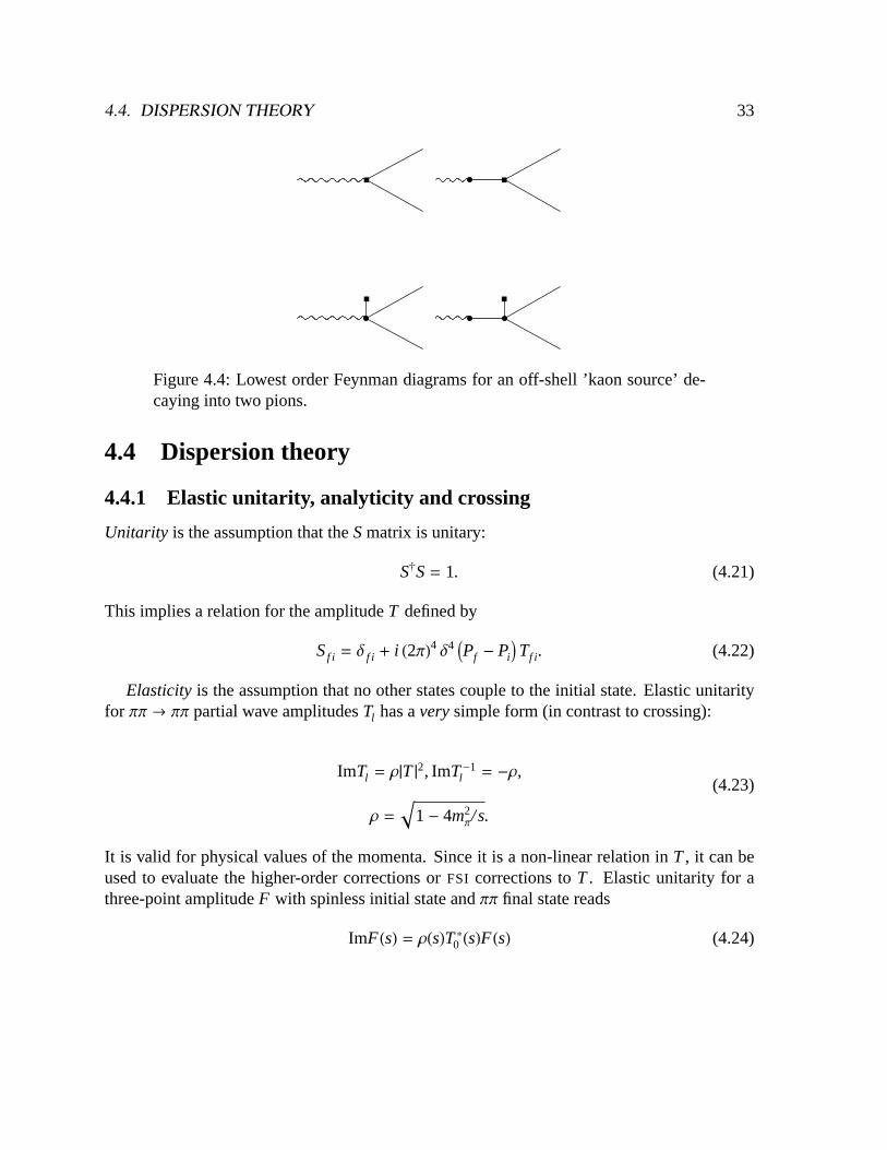
Figure 4.4: Lowest order Feynman diagrams for an off-shell ’kaon source’ de-caying into two pions.
4.4 Dispersion theory
4.4.1 Elastic unitarity, analyticity and crossing
Unitarity is the assumption that theSmatrix is unitary:
SÖS= 1. (4.21)
This implies a relation for the amplitudeT defined by
Sf i = ∆ f i + i (2Π)4 ∆4 IPf - PiMTf i. (4.22)
Elasticity is the assumption that no other states couple to the initial state. Elastic unitarityfor ΠΠ ® ΠΠ partial wave amplitudesTl has averysimple form (in contrast to crossing):
ImTl = Ρ|T |2, ImT-1
l = -Ρ,
Ρ =
1
1- 4m2Π/s.
(4.23)
It is valid for physical values of the momenta. Since it is a non-linear relation inT, it can beused to evaluate the higher-order corrections orFSI corrections toT. Elastic unitarity for athree-point amplitudeF with spinless initial state andΠΠ final state reads
ImF(s) = Ρ(s)T*0 (s)F(s) (4.24)

34 CHAPTER 4. FINAL STATE INTERACTIONS IN NON-LEPTONIC KAON DECAYS
As for any process with only aΠΠ final state, solving it with some low orderF as input pro-vides a means of evaluating a certain class of higher order corrections toF ; the so-calledFSI
or unitarity corrections coming from the interactions of the two pions: (4.24) allows the re-summation of the final state diagrams toall orders, but does not tell us anything about thecontributions from diagrams where the initial particle or source couples via higher order ver-tices to the two final pions. That is, given enough information on theΠΠ amplitude, we canresum all contributions from the right-hand blob of the "cut" diagram of fig.4.5. For the left-hand vertex we must provide the input, e.g. usingCHPT to some order. Contributions thatcannot be "cut" in this way are not addressed by this method. For the case of theI = 0 s-waveit is known [GM91a] that the final state interactions are very strong and dominate the higherorder corrections.
Crossing symmetry(or just crossing) entails the following: With the corresponding choiceof momenta and quantum numbersp1, p2, . . ., oneamplitudeT(p1, p2, . . .) describes the pro-cesses in all channels obtained by interchanging the particles (and changing the sign of theamplitude appropriately).
Analyticity is the assumption that a scattering or decay amplitudeT is an analytic functionof Lorentz invariant variables, e.g. the Mandelstam variabless, t, u, except for the cuts andsingularities demanded by kinematics and resonance poles, unitarity and crossing. E.g. for thecase ofΠK ® ΠK, the amplitudeT(s, t, u) is said to besu-crossing symmetric; it describesΠK ® ΠK in both thes- andu-channel andΠΠ ® KK scattering in thet-channel with thevariables in the regimes of fig.4.6. Between the physical regionsanalytic continuationhas tobe used.
Figure 4.5: "Cut" unitarity diagrams for a three-point amplitude.
4.4.2 Dispersion relations for scattering amplitudes
Consider some scattering process 1+ 2® 3+ 4. It is convenient to specialize to the center ofmass system and define the magnitude of the initial and final three-momentaq, q¢ and cosine

4.4. DISPERSION THEORY 35
of the scattering anglez. One then has
s= J1
q2(s) +m2
1 +
1
q2(s) +m2
2N2= J
1
q¢2(s) +m2
3 +
1
q¢2(s) +m2
4N
2,
t = J1
q¢2(s) +m2
3 -
1
q2(s) +m2
2N
2- q2
(s) - q¢2(s) + 2q
(s)q¢
(s)z(s),
u = J1
q¢2(s) +m2
3 -
1
q2(s) +m2
1N
2- q2
(s) - q¢2(s) - 2q
(s)q¢
(s)z(s),
(4.25)
with solutions
q2(s) =
Bs-(m1+m2)2FBs-(m1-m2)
2F
4s , q¢2(s) =
Bs-(m3+m4)2FBs-(m3-m4)
2F
4s ,
z(s) =
s(t-u)-Jm21-m2
2NJm23-m2
4N
4sq(s)q¢
(s),
(4.26)
and similarly in the other channels (denoted by the subscript). From these equations one easilyfinds the regions of the physical processes in the three crossed channels. For the case ofΠKscattering these regions are displayed in fig.4.6.
Dispersion relations are useful tools in relating the different energy regimes of amplitudes.Their application relies on the assumption of certain analyticity properties of the amplitudes,namely that the amplitudes have no other singularities than the ones arising from the singulari-ties due to the kinematical right-hand cut and the exchange of particles in the direct and crossedchannels. E.g. for elastic scattering of two particles of massesm1 andm2, su-crossing impliesthat theu-channel cut atu > (m1+m2)
2 translates into ans-channel cut atu < (m1-m2)2 since
s+ t + u = 2m22 + 2m2
2 Þ s- 2q2(1- z) + u = 2m2
1 + 2m22. For partial waves, similar consider-
ations show that poles in crossed channels give singularities on the cuts of thes-channel. Forelastic scattering of two particles with different masses, the cut structure of the partial waves isdisplayed in fig.4.7. Since the singularity structure is known, one can use Cauchy’s theoremfor the amplitudeTl to write
Tl (s) =1
2Πi àC
T (s¢)ds¢
s¢ - s, (4.27)
where C is some integration contour enclosing the singularities. If one further assumes suf-ficiently fast fall-off of Tl , contributions from circles at infinity can be dropped leaving thecontour enclosing the singularities.
For the case of elasticΠΠ scattering, as we have seen in section2.6, the scattering amplitudeT I
l (s, t, u) displays full crossing symmetry and has only a left- and a right-hand cut,[-¥, sL]
and[sR,¥] respectively. In the case of fixedt, sL = -t, sR = 4m2Π. For partial waves,sL =

36 CHAPTER 4. FINAL STATE INTERACTIONS IN NON-LEPTONIC KAON DECAYS
-100
0
100
-100
0
100
Figure 4.6: Kinematical boundaries of the Mandelstam variables,s, t, uin unitsof MeV2 for elastic pion kaon scattering.
0, sR = 4m2Π. If T does not fall of sufficiently fast towards infinity (4.27) must be modified:
Assuming thatT Il approaches a constant at infinity, asubtractionats= s0 must be made,
T Il (s) = T I
l (s0)+
s-s0Π Ù
sL
-¥
ImT Il (s¢)
(s¢-s)(s¢-s0)ds¢ + s-s0
Π Ù
¥
sR
ImT Il (s¢)
(s¢-s)(s¢-s0)ds¢,
(4.28)
where we have used the following property of the amplitude:
ImT(s) - ImT(s*) = 2ImT(s). (4.29)
This dispersion relation (withI = l = 1), with simple resonance form input in the crossedchannels, was used in the sixties in the failed attempts, referred to in section2.1, to use disper-sion relations for dynamical calculations. This failure indicated that the left-hand cut structureneeded to reproduce the physical amplitude was more subtle than what could be parameterizedwith a few resonances. A much more successful program was the use of dispersion relations inconjunction with experimental data as a way of analytically continuing the amplitudes beyondthe experimentally accessible regions. In particular, the set of coupled dispersion equations
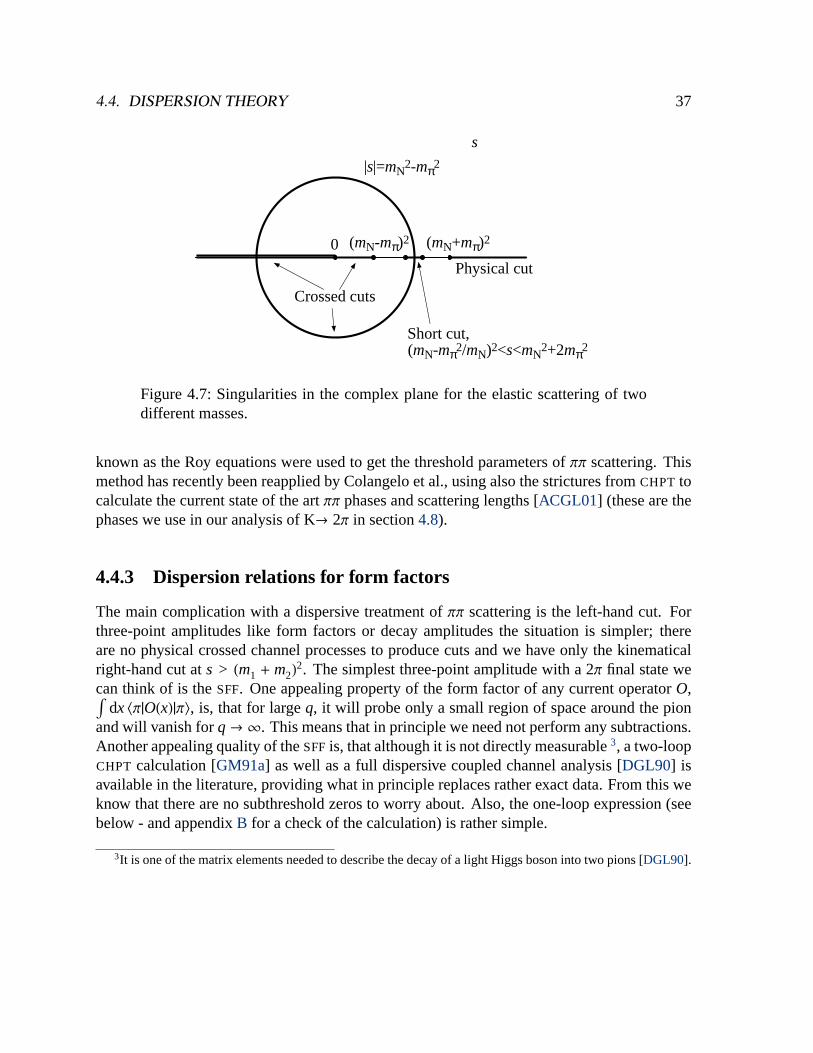
4.4. DISPERSION THEORY 37
Crossed cuts
Physical cut
Short cut,(mN-mπ2/mN)2<s<mN
2+2mπ2
|s|=mN2-mπ2
0 (mN-mπ)2 (mN+mπ)2
s
Figure 4.7: Singularities in the complex plane for the elastic scattering of twodifferent masses.
known as the Roy equations were used to get the threshold parameters ofΠΠ scattering. Thismethod has recently been reapplied by Colangelo et al., using also the strictures fromCHPT tocalculate the current state of the artΠΠ phases and scattering lengths [ACGL01] (these are thephases we use in our analysis of K® 2Π in section4.8).
4.4.3 Dispersion relations for form factors
The main complication with a dispersive treatment ofΠΠ scattering is the left-hand cut. Forthree-point amplitudes like form factors or decay amplitudes the situation is simpler; thereare no physical crossed channel processes to produce cuts and we have only the kinematicalright-hand cut ats > (m1 +m2)
2. The simplest three-point amplitude with a 2Π final state wecan think of is theSFF. One appealing property of the form factor of any current operatorO,Ù dx XΠ|O(x)|Π\, is, that for largeq, it will probe only a small region of space around the pionand will vanish forq® ¥. This means that in principle we need not perform any subtractions.Another appealing quality of theSFFis, that although it is not directly measurable3, a two-loopCHPT calculation [GM91a] as well as a full dispersive coupled channel analysis [DGL90] isavailable in the literature, providing what in principle replaces rather exact data. From this weknow that there are no subthreshold zeros to worry about. Also, the one-loop expression (seebelow - and appendixB for a check of the calculation) is rather simple.
3It is one of the matrix elements needed to describe the decay of a light Higgs boson into two pions [DGL90].

38 CHAPTER 4. FINAL STATE INTERACTIONS IN NON-LEPTONIC KAON DECAYS
We may write an unsubtracted dispersion relation,
Fs(s) =1Πà
¥
sR
ImFs (s¢)
s¢ - sds¢, (4.30)
wheresR = 4m2Π. The question here is then how to get ImFs on the (right-hand) cut. This is the
subject of the next section, where we shall consider a systematic way of resumming the chiralseries using unitarity4.
4.5 The Omnès method
4.5.1 General theory
Consider a three-point amplitudeF like theSFFor the K® ΠΠ amplitude. Assume analyticity,elastic unitarity and that only one subtraction is needed. Then
F(s+ iΕ) º F(s) = F(s0) +1Π Ù
ds¢ J ImF(s¢)(s¢-s) -
ImF(s¢)(s¢-s0)
N
= F(s0) +s-s0Π Ù
ds¢ ImF(s¢)(s¢-s)(s¢-s0)
,
(4.33)
wheres0 is an arbitrary subtraction point. Inserting a complete set of states, ImF can beidentified with the spectral functionΣ [Omn58, Mus53, Bar65],
ImF(s) = Σ(s) =12â
n
YΠΠ; sÄÄÄÄÄ
FÖÄÄÄÄÄ
n] Xn|K; s\ , (4.34)
4An alternative approach is the so-called inverse amplitude method: Perturbative elastic unitarity, as satisfiedby CHPT, reads
ImF (0) = 0, ImF (2) = ΡT0 (2)
0 , . . . . (4.31)
Using this together with exact elastic unitarity and chiral expansion ofT0
0 /F one gets the [0,1], [0,2], ... Padéapproximants ofF ,
F[0,1](s) =
11-F (2)(s)
,
F[0,2](s) =
11-F (2)(s)+F (2)(s)2-F (4)(s)
, . . . .
(4.32)
Gasser and Meissner showed in [GM91a] that if one expands these amplitudes inp the coefficients on the chirallogs come out wrong as compared to the true chiral expansion. What this means is that the Padé approximants donot resum the chiral series and are therefore of no help in evaluating the constants of the chiral lagrangians. Theycan be seen as aCHPT inspired parameterization of the form factor.
4.5. THE OMNÈS METHOD 39
whereF is the scattering operator, all states are "in" states andn is a state which couples toboth the final and initial state. Below the first inelastic threshold the only such state isΠΠ (seefootnote2 in section2.6), wherefore
ImF(s) = Ρ(s)T*0 (s)F(s)
= Ρ(s)T0(s)F*(s)
= ei∆(s) sin(∆(s))F*(s),
(4.35)
where∆ is theΠΠ scattering phase-shift. This leads to the famous Omnès equation [Omn58,Mus53, Bar65]
F(s) = F(s0) +s- s0
Πà
¥
4m2Π
ds¢tan∆(s¢)ReF(s¢)(s¢ - s)(s¢ - s0)
. (4.36)
The solution reads [Omn58, Mus53, Bar65]
F(s) = P(s)exp: s-s0Π Ù
¥
4m2Π
ds¢ ∆(s¢)(s¢-s)(s¢-s0)
>
º P(s) Ws0(s).
(4.37)
The twice subtracted solution reads
F(s) = P(s)exp:F ¢(s0) (s-s0)
F(s0)>exp: (s-s0)
2
Π Ù
¥
4m2Π
ds¢ ∆(s¢)(s¢-s)(s¢-s0)
2>
º P(s)exp:F ¢(s0) (s-s0)
F(s0)>W
(2)s0(s).
(4.38)
Since we assume that there are no other singularities than the cut,P(s) is an arbitrary poly-nomial factor.F has the phase ofT0. This is known as Watson’s final state theorem. IfF(s)happens to be vanish linearly ats = s0, a small modification is necessary; the zero must befactored out:
F(s) = (s- s0)F(s), (4.39)
and the same method applied toF , giving
F(s) = (s- s0)P(s)Ws0(s). (4.40)
If the subtraction polynomialP(s) can be determined,F(s) is known everywhere. We can thendistinguish two cases:

40 CHAPTER 4. FINAL STATE INTERACTIONS IN NON-LEPTONIC KAON DECAYS
1) F(s0) ¹ 0.
P(s) = P(s0) + P¢(s0)(s- s0)
= F(s0) + (F¢(s0) - F(s0)W
¢
s0(s0))(s- s0)
(4.41)
2) F(s0) = 0.P(s) = F ¢(s0) (4.42)
In either case the input isF(s0) andF ¢(s0).
4.5.2 TheSFF
As mentioned, theSFF is well under control both from a chiral and an "experimental" pointof view. To get an understanding of theFSI it is instructive to rewrite the one-loop expression(4.10) as
G(s) º Fs(s)/Fs(0) = 1+ cs+s2
Πà
¥
4m2Π
ds¢∆
0 (2)0 (s¢)
s¢2(s¢ - s)+ O(s3
), (4.43)
wherec is a constant related to theLi ’s ~ ln m2Π, which can be fixed from the scalar radius of
the pion.∆0 (2)0 is theLO ΠΠ phase-shift in the s-wave,I = 0 channel
∆00(s) = ∆
0 (2)0 (s) + ∆
0 (4)0 (s) + . . . ,
∆0 (2)0 (s) = ΠΣ(s)
32Π2 f 2Π
(2s-m2Π),
(4.44)
with Σ(s) =1
1- 4m2Π/s. Since there is no zero ofG at s = 0 and only one subtraction is
needed, we can use (4.37) with s0 = 0 andP(s) = 1. In practise one then needs to cut off theintegral at some valueL2 high enough that the result depends very little on the precise value.In fig. 4.8 this is displayed, using a cut-offL = 1.4GeV and the phase-shift of [CGL01a],together with the three first orders ofCHPT and the "true form factor" [DGL90] referred to insection4.4.3. At s= m2
K = 0.498 GeV the chiral series looks as follows:
1 (LO) ® 1.62 (NLO) ® 1.67 (NNLO)
® 1.42 ("true value").
(4.45)

4.5. THE OMNÈS METHOD 41
0 0.1 0.2 0.3 0.4 0.5
E (GeV)
0.8
1
1.2
1.4
1.6
1.8
Re[
FS(s
)]
CHPT LO
CHPT NLO
CHPT NNLO
Omnes - sharp cutoff at 1.4 GeV
Figure 4.8: Scalar form factor: Comparison of theCHPT calculation to leading,next-to-leading and next-to-next-to-leading order and the dispersive one (seelegenda). The solid curve is the "true form factor", see text.
We observe that the bending of the "true form factor" is reproduced byCHPT only at next-to-next-to-leading order (NNLO) and then shifted right. This, however, can be easily understoodby observing that
ReG(s) ~ cos∆(s) ~ 1-∆(s)2
2+ . . . , (4.46)
and that, since the phase is a quantity of orderp2 in the chiral expansion, the negative part,responsible for the bending down, starts atNNLO and will thus have sizeable contributionsfrom even higher orders.
From the previous paragraphs, we conclude thatFSI can indeed shift the leading order resultsubstantially,~ 50%, and that this effect is primarily carried by the one-loop correction, butthat higher orders can modify the one-loop prediction by another~ 15%.
4.5.3 K® 2Π
Armed with the knowledge thatFSI are indeed important for three-point amplitudes with s-waveΠΠ final state, we proceed now to the decay K® 2Π. Ignoring for the moment thatthe constantc5 of the LO weak chiral lagrangian and the constants of theNLO weak chirallagrangian are largely unknown, at small values ofs, CHPT is reliable and can be used fordeterminingA and the slope ofA; we shall use the two amplitudes defined in (4.17) and (4.18).The twoCHPT amplitudes have zeros at rather unsuitable values ofs: The right-and side of

42 CHAPTER 4. FINAL STATE INTERACTIONS IN NON-LEPTONIC KAON DECAYS
(4.17) has a zero atc23m2
Πm2
K + c5m2K(2m2
K -m2Π)
c23m2K + c5(2m2
K -m2Π)º sP
0, (4.47)
dependent onc5. The right-hand side of (4.18) has a zero at
2m2Π-m2
K º sA0 , (4.48)
Using (4.17), (4.47) and (4.39), setting c5 to zeroand subtracting ats0 = m2Π, we get5
ÄÄÄÄÄ
A Im2KMÄÄÄÄÄ
/c2 = 823 GeV-1. (4.49)
This is the result of [PP00]. Subtracting instead ats0 = 0, we getÄÄÄÄÄ
A Im2KMÄÄÄÄÄ
/c2 = 941 GeV-1. (4.50)
This is the result of [PP01]. If c5 is not set to zero, but instead to e.g. 0.1c2 and the subtractionis made ats0 = sP
0, we getÄÄÄÄÄ
A Im2KMÄÄÄÄÄ
/c2 = 875 GeV-1. (4.51)
Using (4.18) and (4.48) and subtracting ats0 = m2Π, we get
ÄÄÄÄÄ
A Im2KMÄÄÄÄÄ
/c2 = 477 GeV-1. (4.52)
It is seen that using the (pseudo-scalar) off-shell amplitude (4.17), modifies the result of [PP00]by 6 % withc5 = 0.1c2. It is also seen that using the (axial-vector) off-shell amplitude (4.18),gives a result which differs from the result of [PP00] by 58 %. In this case, it should be notedthat the difference is due to the term proportional toW¢(m2
Π) which is of one order higher in the
chiral expansion than the rest.These simple examples spotlight the perils of using (weak)CHPT for fixing subtraction
constants in a dispersive treatment of K® 2Π: In contrast to the case of theSFF, there is noobservable quantity which can be used for fixing the subtraction constants; that is, the couplingconstants of the weak chiral lagrangians are largely unknown, even those of theLO lagrangian.Moreover, the off-shellCHPT amplitudes are not uniquely defined and cannot be used to fixsubtraction constants in a dispersive representation. In other words,AK®ΠΠ
(s) is ill-suited fordispersive treatment because the subtraction point must be made in an off-shell region whereit is ambiguous.
In section4.7an alternative method is proposed which avoids this problem. First however,we need to introduce some additional tools.
5The experimental input used is:fΠ= 92.4 MeV, m
Π= 139.57 MeV, mK = 495.67 MeV and the phase-shift analysis of [AMP87]. The value of
fΠ
is the one used in [PP01].

4.6. THE SOFT PION THEOREM FOR NON-LEPTONIC KAON DECAYS 43
4.6 The soft pion theorem for non-leptonic kaon decays
4.6.1 Allowing the weak lagrangian to carry momentum
The generating functional reads
W[ jV , jA, js, jp] = Ù [dU]ei Ù dx(LS+LW
+VΜ
jΜ
V+...). (4.53)
Since the weak coupling is indeed very weak, we need keep only linear terms inLW,
W[ jV , jA, js, jp] =
Ù [dU]ei Ù dx(LS+VΜ
jΜ
V+...)(1+ i Ù dxLW
+ . . .).
(4.54)
We may viewLW like any other operator whose expectation values can be calculated fromW.To this end we couple it to a source, i.e. allow it to carry momentumq. The CP conservingDS = 1 weakCHPT lagrangianLW, which we are considering, can be viewed as the sixthcomponent of an isoscalar operator octet, and can thus be coupled to a multiplet of externalsourcesj i
W. To achieve this we substituteΛ6 ® j iWΛi. Thus instead of (4.16) we shall use
LW,2 = c2 X jiWΛiDΜU
ÖDΜU\ + c5 X jiWΛi I
ÖΧ + Χ
ÖUM\ . (4.55)
There is of course no field in nature corresponding toj iW, that is, the Green’s functions with
qΜ ¹ 0 are well-defined but unphysical objects. SettingqΜ = 0 is the physical limit.The amplitudes we shall need for our discussion of the soft pion theorem are the Kl ® Π
0
and Ks® Π0Π
0 amplitudes, both with a momentum carrying weak lagrangian. More precisely,we define
X(q2) º
1
(-2 fΠB0)
2 limk2®m2
Kp2®m2
Π
(k2-m2
K)(p2-m2
Π)Ξ
63(k2, p2, q2
), (4.56)
with
Ξ63(k2, p2, q2
) º
i Ù d4xÙ d4yÙ d4z eik×xeip×yeiq×zZ0ÄÄÄÄÄÄ
T :P6Ö(x)P3
(y)LW(z)>ÄÄÄÄÄÄ
0^ ,
(4.57)

44 CHAPTER 4. FINAL STATE INTERACTIONS IN NON-LEPTONIC KAON DECAYS
and
T+(s, t, u, q2) º
1(-i f
ΠpΜ)(-2 f
ΠB0)
2 limk2®m2
K
p21®m2
Π
p22®m2
Π
(k2-m2
K)(p21 -m2
Π)(p2
2 -m2Π)Τ
733Μ(s, t, u, k2, p2
1, p22, q2),
(4.58)
with
Τ733Μ(s, t, u, k2, p2
1, p22, q2) º ià
d4xà
d4y1à d4y2à d4z
eik×xeip1×y1eip2×y2eiq×zZ0ÄÄÄÄÄÄ
T :A7ÖΜ(x)P3
(y1)P3(y2)L
W(z)>ÄÄÄÄÄÄ
0^
(4.59)
ands, t, uthe usual Mandelstam variables
s= (p1 + p2)2, t = (q+ p1)
2, u = (q+ p2)2 , (4.60)
where all momenta considered incoming, related bys+ t + u = 2m2Π+ m2
K + q2, with q themomentum carried by the weak Hamiltonian. From now on we setq2
= 0 (but qΜ ¹ 0 ingeneral).
4.6.2 The soft pion theorem
First we consider a general matrix element involving a soft pion [LSZ55],
XΠi(p)B|O(0)|A\ = i Ù d4xeip×x
(2 +m2Π) XB|TΠi
(x)O(0)|A\
= Ù d4xeip×x(-p2
+m2Π) XB|T 9Πi
(x)O(0M}|A\ ,
(4.61)
whereA andB denote two arbitrary ensembles of particles,Πi a pion with isospin indexi,which is to be taken off-shell,p® 0, andO is some operator. According to the Haag theorem(see section2.5), we can make thePCAC choice
Πi=
1
fΠm2Π
¶ΜAiΜ, (4.62)

4.6. THE SOFT PION THEOREM FOR NON-LEPTONIC KAON DECAYS 45
whereAiΜ
is the isospini axial-vector current operator. From the above two equations follows
YΠi(p)B|O(0)|A] = i m2
Π-p2
fΠm2Π
Ù d4xeip×xYB|T 9¶ΜAi
Μ(x)O(0)= |A]
= i m2Π-p2
fΠm2Π
Ù d4xeip×x
YB|Θ(x0)¶ΜAiΜ(x)O(0) - Θ(-x0)O(0)
ΜAiΜ(x)|A]
= i m2Π-p2
fΠm2Π
Ù d4xeip×x
I¶ΜYB|T 9Ai
Μ(x)O(0)= |A] - ∆(x0) YB| AA
i0(x), O(0)E |A]M
= i m2Π-p2
fΠm2Π
Ù d4xeip×x
I-ipΜ YB|T 9AiΜ(x)O(0)= |A] - ∆(x0) YB| AA
i0(x), O(0)E |A]M ,
(4.63)
where we have used integration by parts and the fact that the derivative of the Heavyside stepfunctionΘ is the Dirac delta function∆. We now take the limitqΜ ® 0 by first settingq = 0and then lettingq0 ® 0, whereby we get the soft pion theorem,
XΠi(p = 0)B|O(0)|A\ = - i
fΠ
XB| AQi5, O(0)E |A\ + i limpΜ®0 pΜRi
Μ,
RiΜ= -
ifΠÙ d4xeip×x
XB|T 9AiΜ(x)O(0)= |A\ .
(4.64)
The last term vanishes unlessRiΜ
has a singularity atqΜ = 0. This is the case e.g. for the matrixelements considered in Kl4 decays as noted by Weinberg in [Wei66]. The soft pion theoremis exact at theSPP, p
Μ= 0, and relates one state|B\ to another state|Πi
pΜ=0B\ obtained by the
addition of a zero-energy Goldstone pion. When going away from the SU(2) chiral symmetrylimit to the real world,q2
= m2Π, corrections of orderm2
Πcan be expected [GL84].
Now we want to apply the soft pion theorem to the case of Ks ® 2Π0. For the amplitude
46 CHAPTER 4. FINAL STATE INTERACTIONS IN NON-LEPTONIC KAON DECAYS
T+(s, t, u, q2) of (4.58) we get
T+(s= m2Π, t = m2
K, u= m2Π, q2= 0) = YΦ3
|H6W(0)|Φ
7Φ
3]
= -ifΠ
Y0| AQ35,H
6W(0)E |Φ
7Φ
3] = -
ifΠ
Y0| AQ35,H
7W(0)E |Φ
6Φ
3]
= -1
2 fΠ
Y0|H6W(0)|Φ
6Φ
3] = -
12 fΠ
X(q2),
(4.65)
where we have used the fact thatH iW(0) is an SU(3) octet and obeys the algebra
BQi5,H
jW(0)F = i f i jkH
kW(0). (4.66)
(4.65) can be considered accurate up toO(m2Π) because it is based on the soft pion theorem.
In contrast hereto, theCHPT prediction at the physical point,q2= 0, s = m2
K, t = m2Π, u = m2
Π,
suffers fromO(m2K) corrections. MoreoverT+(s, t, u) is well-suited for dispersive treatment
because the continuation from theSPP to the physical point is done in the on-shell regionwhere it is well-defined.
We have checked the that the relation (4.64) is satisfied by theCHPT amplitudes of sectionC.2.
4.7 Crossed channel dispersion equations
Since the weak Hamiltonian has the quantum numbers of the kaon, and the pions are in anisospin zero state,T+(s, t, u) is analogous to thet W u even combination of the KK® ΠΠscattering amplitude (the notation is borrowed from ref. [Lan78]). Like in that case, one canshow that if one neglects the imaginary parts of d-waves and higher in all channels, then theanalytic structure of the amplitude simplifies and it can be decomposed into a combination offunctions of a single variable (for the KΠ scattering case see [AB01]):
T+(s, t, u) = M0(s) +13 AN0(t) + N0(u)E +
23 AR0(t) + R0(u)E
+12 BJs- u- m2
ΠD
t NN1(t) + Js- t - m2ΠD
u NN1(u)F ,
(4.67)

4.7. CROSSED CHANNEL DISPERSION EQUATIONS 47
whereD = m2K - m2
Π. Notice that the terms proportional toN1 drop out in the physical decay
amplitude:
AK®ΠΠ = T+(m2K, m2
Π, m2Π) =
= M0(m2K) +
23 AN0(m
2Π) + 2R0(m
2Π)E .
(4.68)
Each of the single variable functions appearing in equation (4.67) is analytic in the complexplane except for a cut starting at 4m2
Πfor M0 and at(mK +m
Π)2 for the remaining ones. These
functions are defined to have the discontinuity on the positive real axis identical to that of aspecific partial wave:M0 to theI = 0 S-wave in thes-channel, whereas in thet-channel,N0andN1 to theI = 1/2 s- and p-wave respectively, andR0 to theI = 3/2 s-wave6. Below theinelastic threshold, the elastic unitarity condition for these functions reads
discM0(s) = sin∆00(s)e-i∆
00AM0(s) + M0(s)E ,
discNl(s) = sin∆1/2l (s)e
-i∆1/2lANl(s) + Nl(s)E ,
discR0(s) = sin∆3/20 (s)e
-i∆3/20AR0(s) + R0(s)E ,
(4.69)
where∆00 is theΠΠ phase-shift, whereas those with half-integer isospin are theΠK phase-shifts.
The "hat functions" denote contributions from the other channels contributing via angular
6We disregard the imaginary part of theI = 3/2 p-wave in thet-channel because it is phenomenologicallyvery small and vanishes in the chiral expansion up to orderp6.

48 CHAPTER 4. FINAL STATE INTERACTIONS IN NON-LEPTONIC KAON DECAYS
averages (to be specified below). They are defined by
M0(s) = AsS1 - 2m2Km2Π-
14(m
4K + 3s2
)E XN1\ + 2s|p||q|XzN1\
+4|p|2|q|2Xz2N1\ +23(XN0\ + 2XR0\),
N0(t) = XM0\s+ y(t)XM1\s- r(t)XzM1\s+13 I4XR0\u - XN0\uM
-18w(t)XN1\u -
14v(t)XzN1\u +
18r2(t)Xz2N1\u,
N1(t) =2
r(t) 9XzM0\s+ y(t)XzM1\s- r(t)Xz2M1\s
+13 I4XzR0\u - XzN0\uM -
18w(t)XzN1\u
-14v(t)Xz2N1\u +
18r2(t)Xz3N1\u=
R0(t) = XM0\s-12y(t)XM1\s+
12r(t)XzM1\s+
13 IXR0\u + 2XN0\uM ,
+14w(t)XN1\u +
12v(t)XzN1\u -
14r2(t)Xz2N1\u,
(4.70)
where
N1(t) = N1(t)/t, S = m2K +m2
Π,
S1 = S +m2Π, y(t) = S1 - 3t - m2
ΠD
t ,
ΡΠK(t) =
1
I1- (mK +mΠ)2/tM I1- (mK -m
Π)2/tM,
r(t) = (t -m2Π)ΡΠK(t), v(t) = Jt - m2
ΠD
t N r(t),
w(t) = 3t2- 4tS1 + 5m4
Π+ S
2-
m4ΠD
2
t2 .
(4.71)
X\ indicate angular averages defined by
XznX\(s) = 12 Ù
1
-1dzznX(S1/2- s/2+ 2|p||q|z),
XznX\v(t) =12 Ù
1
-1dzznX(v(t, z)), v = s, u,
(4.72)

4.7. CROSSED CHANNEL DISPERSION EQUATIONS 49
where
|p|2 = s4 -m2
Π, |q|2 = s
4 J1-m2
Ks N
2,
s+ u = S1 - t, s- u = m2ΠD
t + r(t)z.
(4.73)
In the definition of the "hat functions" the functionM1 appears. This function is analogous toM0 in the case of theI = 1 p-wave in thes-channel, and is necessary to describe theT+(s, t, u)in full generality, for all channels (including thet W u odd, I = 1 s-channel). It does notcontribute directly to the physical decay process: Its indirect (and small) contribution via theangular average in the dispersion relation is a consequence of crossing symmetry.
If one is only interested in the low-energy region, neglecting the inelastic channels is a goodapproximation. Then the solution of the dispersion relation for each of the functions is wellapproximated by the Omnès function times a polynomial [Omn58]. It is therefore convenientto write the dispersion relation for the functions divided by the corresponding Omnès function(see [AL96] for a detailed discussion of this point, although in a different framework) in thefollowing form:
M0(s) = W00(s, s0) 9a+ b(s- s0)+
(s-s0)2
Π Ù
L21
4m2Π
sin∆00(s¢)M0(s¢)ds¢
|W00(s¢,s0)|(s
¢-s)(s¢-s0)
2? ,
N0(s) = W1/20 (s);
s2
Π Ù
L22
(mK+mΠ)2
sin∆1/20 (s¢)N0(s
¢)ds¢
|W1/20 (s¢)|(s¢-s)s¢2
? ,
N1(s) = W1/21 (s);
sΠ Ù
L22
(mK+mΠ)2
sin∆1/21 (s¢)N1(s
¢)ds¢
|W1/21 (s¢)|(s¢-s)s¢
? ,
R0(s) = W3/20 (s);
s2
Π Ù
L22
(mK+mΠ)2
sin∆3/20 (s¢)R0(s
¢)ds¢
|W3/20 (s¢)|(s¢-s)s¢2
? .
(4.74)
WIl (s) is the Omnès function [Omn58], defined by
W00(s, s0) = exp; (s-s0)
Π Ù
L21
4m2Π
ds¢ ∆00(s¢)
(s¢-s0)(s¢-s)? ,
WIl (s) = exp; s
Π Ù
L22
(mK+mΠ)2 ds¢ ∆
Il (s¢)
s¢(s¢-s)? , I = 12, 3
2.
(4.75)
All functions are subtracted ats= 0 except forM0, for which the subtraction points0 is leftunspecified. In the following we uses0 = m2
Π. The fact that onlyM0 depends on subtraction
constants does not have any deep reason: The splitting of polynomial terms ofT+ between

50 CHAPTER 4. FINAL STATE INTERACTIONS IN NON-LEPTONIC KAON DECAYS
the various functionsM0, N0,1 andR0 is arbitrary, and we have merely used this freedom toremove them from the latter three. The final result does not depend on this choice [AL96]. Allthe dispersive integrals above have been cut off at energiesL1,2 andL1,2 - numerical valueswill be given below.
4.8 Solving the equations
If the ΠΠ and KΠ phase-shifts, the cutoffsL1,2, and the subtraction constantsa andb are given,the dispersion relations (4.74) can be solved numerically. Such a solution gives the amplitudeT+(s, t, u) at any point (provided it is far enough from the inelastic thresholds) of the Mandel-stam plane, in particular at the physical point. The crucial new input here are the two subtrac-tion constants. The phase-shifts are known with sufficient accuracy, whereas the choice of thecutoffs is dictated by the inelastic thresholds. Before proceeding we have to discuss how thesetwo subtraction constants can be determined. If they could be calculated with better accuracythan the physical amplitude itself, it would represent a clear advantage for our method.
For one of the two subtraction constants this is the case. The soft-pion theorem relates theamplitude at theSPPto the K® Π amplitude up to terms of orderm2
Π. We can therefore write
-1
2 fΠ
AK®Π = a+13AN0(m
2K) + 2R0(m
2K)E + O(m
2Π), (4.76)
which shows thata is indeed directly related to a quantity that is calculable (more easily thanthe decay amplitude itself), e.g. on the lattice. The relation (4.76) illustrates the strength of thesoft-pion theorem: Although the process involves a kaon, the relation is based on the use oftheSU(2) symmetry, and therefore suffers from corrections of orderm2
Πonly.
The key to the problem is the calculation ofb. This constant is related to the derivative ins of the amplitudeT+ at theSPP. The calculation ofb requires the evaluation of the physicalamplitudeT+ at an unphysical point, via analytic continuation. While this is easy to do withan analytical method likeCHPT, it is practically impossible with a numerical method likethe lattice method. However there is a Ward identity that relates this derivative to a Green’sfunction which is directly calculable:
¶sT+(s,S - s, m2
Π)|s=m2
Π
=12C(m2
Π, m2
K, m2Π) + O(m2
Π), (4.77)
whereC(s, t, u) is an amplitude defined by
ifΠ
àdxeip1x
XΠ(p2)|TH1/2W (0)A
Μ(x)|K(q1)\ = ip
Μ
1B+ iqΜ
1C+ iqΜ
2D , (4.78)

4.8. SOLVING THE EQUATIONS 51
whereAΜ(x) is the axial current that couples to the pion removed from the outgoing state. Bymaking the momentump2 soft, one can also derive a soft-pion theorem which relates the four-point function in equation (4.78) to a three-point function. Unfortunately the functionC cannotbe singled out from this relation.
We are not aware of any attempts to calculateb. In order to illustrate our method we proceedby fixing b at a certain value and then varying it within a fairly wide range. To fix the centralvalue and the range we useCHPT as a guide. At leading order,CHPT dictates the followingrelation betweena andb:
b =3a
m2K -m2
Π
I1+ X + O(m4K)M . (4.79)
The size of the correction is at the moment unknown, but nothing prevents it from being oforderm2
K: X = m2K/ (16Π2F2
K )x, with x expected to be of order one. An explicit calculation inCHPT (see sectionC.2) yields7:
x = 3839 -
802154 log 4
+13 log m2
K
m2Π
-83(N5 + 2N7 - N9 - 4N10- 4N11)
+2(N19- N20) -43(2N21+ N22+ 2N23) + O J
m2Π
m2KN ,
(4.80)
whereNi = 16Π2Nri (mK) are the renormalized low-energy constants introduced in [EKW93].
Since we lack information on many of the constants, theCHPT calculation (4.80) does notallow us to do more than an order of magnitude estimate forb. In our numerical study wehave usedX = ±30%. The normalization of the amplitude is irrelevant here, and we havefixed it atT+(m2
Π, m2
K, m2Π) = 1. For the cutoffs we have usedL1 = 1 GeV,L2 = 1.3 GeV, and
Li = 1.05Li. Our results8 are shown in fig.4.9, where we have plotted|T+(s,S-s, m2Π)| versus
s, comparing our numerical solution of the dispersion relations to theCHPT leading orderformula. The latter is what has been used so far whenever a number for the K® ΠΠ matrixelement extracted from the lattice has been given. Our treatment shows that large correctionswith respect to leading-orderCHPT are to be expected. One source of large corrections isthe Omnès factor due toΠΠ rescattering in the final state [PP00, Tru88]. The other potentiallydangerous source is represented byX, the next-to-leading order correction to the relation (4.79)betweena andb. The latter could (depending on the sign) in principle double, or to a large
7We have dropped the contribution coming from the weak mass term - more on this below.8The experimental input used is:
mΠ= 139.57 MeV, mK = 497.672 MeV, m
Η= 547.30 MeV, theΠΠ phase-shifts from [ACGL01], the scattering
lengths determined in [CGL00], and theΠK phase-shifts from [JOP00].

52 CHAPTER 4. FINAL STATE INTERACTIONS IN NON-LEPTONIC KAON DECAYS
0.1 0.2 0.3 0.4 0.5
E(GeV)
0
1
2
3
4
5
6
7
8
|T+| Soft-pion point
Physical point
tree level CHPT
dispersive treatment X = 0.0
dispersive treatment X = 0.3
dispersive treatment X =-0.3
Figure 4.9: The function|T+(s, t, u)| plottedvs. E=0
salong the line of constantu = m2
Π. The result of our numerical study for different values ofX are compared
to tree levelCHPT.
extent reabsorb the correction due toFSI. The dependence onX is well described by thefollowing linear formula:
|A(K ® ΠΠ)||ALO CHPT
(K ® ΠΠ)|= 1.5 (1+ 0.76X) , (4.81)
after having normalized both amplitudes toT+(m2Π, m2
K, m2Π) = 1. The evaluation of the un-
certainties to be attached to the numbers in equation (4.81) is in progress. At the moment,however, the main source of uncertainty is the fact thatX is largely unknown.
One of the outcomes of the present analysis is that the effects embodied in the functionsN0,1andR0 have turned out to be very small: If we drop them altogether, the numbers in equation(4.81) change from 1.5 to 1.4 and from 0.76 to 0.75. Notice that these effects are in principleof orderm2
K, as can be seen in equation (4.76), and that they are not a priori negligible. On theother hand this result is very much welcome, because the size of these functions depends bothon theΠK phases (which are less well known than theΠΠ ones) and on the choice of the cutoffL2, which may induce large uncertainties.
4.9. RESULTS AND DISCUSSION 53
4.9 Results and discussion
We have set up a dispersive framework for the K® ΠΠ amplitude that allows evolving theamplitude from the soft-pion point (where it is given by theK ® Π amplitude) to the physicalpoint, taking into account all the main physical effects. As we have pointed out, this evolutionis on safe ground only if a second input is made available: The derivative of the amplitudeat the soft-pion point, which, to the best of our knowledge, has not been calculated so far.We have calculated this second subtraction constant toNLO in CHPT. Given the presenceof unknown low-energy constants, we cannot use this expression for more than an order ofmagnitude estimate. Our numerical work, however, shows that the amplitude at the physicalpoint depends strongly on the value of the slope at theSPP, see fig.4.9and related discussionin the text. A non-perturbative calculation of the second subtraction constantb is necessary inorder to obtain an accurate result with this method. We have provided a Ward identity whichmight be useful in this respect.
Lattice calculations of the K® ΠΠ amplitude made so far [Lel01] rely on tree-levelCHPT
to relate the calculatedK ® Π matrix elements to the physical decay amplitude. The methodproposed here improves this scheme by combining input from the lattice with dispersion re-lation techniques, thereby providing a fully consistent treatment ofFSI in K® ΠΠ. Given thetwo subtraction constants, the dispersion relations can be solved numerically to good accuracy.Recently, a direct calculation of the K® ΠΠ matrix element on the lattice has been proposedin ref. [LL01] - this method does not rely onCHPT. Other lattice methods, which also do notrely on the evaluation of the K® Π amplitude, have also been proposed [D+98]. Each of thesemethods presents different technical problems in its practical implementation [Gol00], and itis difficult to predict which one will lead to a reliable calculation of the K® ΠΠ amplitude. Wehope that the present work will stimulate further efforts to calculate the subtraction constantsa andb, either on the lattice, or by other non-perturbative methods.

54 CHAPTER 4. FINAL STATE INTERACTIONS IN NON-LEPTONIC KAON DECAYS

Chapter 5
Computerized quantum field theory
This chapter contains an introduction to the automatized Feynman diagram calculations usedin the previous chapters. This includes some historical notes and a short review of othercomputerization methods as well as some simple explicit examples of using theMathematicapackageFeynCalc coauthored by the author.
5.1 Introduction
Loop calculations in renormalizable theories
In recent years, a great deal of work has been invested by various groups in the automatizationof Feynman diagram calculations (see [HS99] for a review). The focus has mainly been on per-turbativeQCD [GW73a, GW74, GW73b, Pol73], the electro-weak part of the Standard Model[Gla61, Wei67a, Sal68] and supersymmetric extensions [WZ74, VA73] of it. Electro-weakcalculations are at the two-loop level for correlators (e.g. [WSB94, FHWW00]), but essen-tially still at one-loop level (e.g. [BMR72, DH98, DP01]) for vertex and scattering diagrams.Experiments are however reaching a level of precision demanding higher order calculationsand some have already been done, e.g. the muon anomalous moment to two loops [CKM96](see [CM01b] for an update on the muon anomalous magnetic moment and [GR01] for a gen-eral review of two-loop calculations), but a general method like [tHV79, PV79] is still lacking;thus some integrals have to be done numerically. InQED loop calculations are of course muchsimpler and of older date. The two-loop vacuum polarization was calculated in 1955 [KS55],the two-loop electron self energy in 1962 [Sab62], the anomalous magnetic moment [Sch49]to two loops in 1957 [Pet57], the full two-loop three-point function in 1972 [BMR72] andtwo-loop Bhabha scattering in 2000 [BDG01]. The QED contributions to the quark mass and
55

56 CHAPTER 5. COMPUTERIZED QUANTUM FIELD THEORY
wavefunction renormalization have by now been calculated to three loops on the mass-shell[MvR00] and the anomalous magnetic moment of the electron has been calculated analyti-cally to three loops [LR97] and numerically up to five loops [Kin96, CM99]. QCD calculationsare at two loops for correlator ([FJTV99]) diagrams and some vertex diagrams (e.gZ0 ® bbin the large top mass limit [FTJR92] or the matrix element of the current current operator inb ® sΓ [GHW96, BCMU01]) but are reaching three loops [CKS96, MvR00] and are at fourloops for the beta function [vRVL97] whereas scattering diagrams are at the two-loop level(see [GTY00, Glo01] for an overview). One challenge inQCD and electro-weak calculationsis the enormeous number of Feynman diagrams arising from the many different particles andcouplings. In the proposed supersymmetric extensions of the standard model this problemis all the more acute (see e.g. [HW01, HHRW01, HS01]). The physical motivation for suchcalculations is of course that they are necessary to match the precision of experiments. Moregenerally, these detailed checks are necessary because even though the Standard Model hasnot so far been in disagreement with experiment, it is generally considered unsatisfying as afinal theory and the only obvious way to look for a new theory is to find disagreement betweenthe old theory and experiments and explain these via extensions of the old theory.
Loop calculations in CHPT
Loop calculations inCHPT are necessary because of the level of accuracy direct low energyscattering experiments are reaching [G+01, P+01, Pan99, LMGPNP], but also becauseCHPT
is used as an ingredient in the calculation of important parameters of the Standard Modellike quark masses and the quark vacuum condensate [GL82, CGL01b], CKM matrix elements[KM73, BBJR92] and¶¢/¶ [PP00, PP01, BCKO01a]. Many processes inCHPT have by nowbeen calculated at the two-loop level [GM91a, BCT98, BCE+97, ABT00a, ABT00b, BGS,Bur96, GK95, GK98, DK00]. In one-loop SU(2) mesonicCHPT, the main challenge is not thenumber of Feynman diagrams, but rather the complexity of the counter-term lagrangian. Whengoing to SU(3) and/or two loops however, the number of Feynman diagrams also becomes anissue. Notice that one feature distinguishing effective theories likeCHPT from traditionallyrenormalizable theories is that there is no restriction on the number of legs in vertices (rulingout, for our purposes, all Feynman diagram generating software I know of except forFey-nArts).
Purpose and features of the packagePHI
As is clear from the preceding, loop calculations and in particular more or less computerizedloop calculations is a very active line of research in most field theories. Indeed, the precisionof high energy experiments like the ones atSLC andLEP 1 spurred computational projects like

5.1. INTRODUCTION 57
MADGRAPH [SL94], GRACE [Y+00], COMPHEP [P+99], FeynArts [Hah01] andFeynCalc[RMD91, MBD91b, KEM, Merb, WMSBb, MS98, MO00] of which all but the first one is stillin more or less active development. With the next generation of experiments like the ones atLEP 2 andLHC, some authors argue that it would be desirable to have more collaboration andstandardization between the different projects. Recently a proposal [DKR02] for standardizingthe definition of a field theoretical model has appeared. The proposal is far from perfect orcomplete, but in my opinion a step in the right direction. If all projects would follow such astandard, it would mean that the definition of a model could be written down by one groupin form of anXML [Con] file, immediately processed and used for calculations of amplitudesand sent to other groups that could also immediately process it and use it for calculations ofamplitudes with their different computational software. Of course, to be of real use, such astandard would have to be accompanied by a standard for the notation of amplitudes. Alsorecently a proposal [Tka02] for converging on a common programming language and furthermodularization or componentization of the computational software developed has appeared.One benefit of this would be the easy reuse of code (e.g. a fast algorithm for the evaluation ofDirac traces). While nice, I don’t think this idea has many chances of being adopted generally.
Notice one point: In all the computational projects mentioned except, despite good inten-tions, the specification of a model is a non-trivial undertaking and indeed all projects, exceptfor FeynCalc, deal exclusively with the Standard Model and/or minimal supersymmetric ex-tensions of the Standard Model.
Originally, theMathematica packageFeynCalc was developed for calculating one-loopFeynman diagrams in the electro-weak Standard Model. The input was raw integral expres-sions which can be written by hand or, when too many, produced by e.g. the Feynman diagramgeneratorFeynArts [KEM, HPV99, Hah01]. The output was expressions written in terms ofPassarino-Veltman functions [tHV79, PV79]. This implied implementing kinematical tensorstructures, Dirac algebra etc. Later, general aspects were developed further and some two-loopformalism was also implemented by the original author in connection with perturbativeQCD
calculations [MvN96], and recently (see previous chapters and [BCKO01a]), FeynCalc hasalso been used for some calculations inCHPT.
PHI is aMathematica [Wol00] package for Feynman diagram computations inCHPT. Itis an extension ofFeynCalc and can be used to automatize the most cumbersome tasks in thecalculation of amplitudes.
The motivation for writingPHI was the lack of software for quickly and systematicallyimplementing a quantum field theoretic model; for example an effective model like the variousCHPT models mentioned above which have a more complicated power counting than modelswhich simply expand Green’s functions perturbatively in a coupling constant. However, the

58 CHAPTER 5. COMPUTERIZED QUANTUM FIELD THEORY
package is general enough that other models can easily be specified as demonstrated with thesimple example ofQED (see appendixB). Given the many effective models that already existand the many new ones that keep coming, it is the hope of the author that this software mightbe of use also outside the realm ofCHPT.
The main features ofPHI are:
• A set of basic objects are provided that can be composed and manipulated to formCHPT
lagrangians.
• The most commonCHPT lagrangians are included and new ones can easily be defined.
• The lagrangians can be expanded in terms of pion (meson) fields, with SU(2) (SU(3))flavour traces being done automatically.
• External sources can be switched off and on.
• Compatibility with FeynArts for generation of Feynman diagrams and amplitudes in-cluding counter-terms. Power counting and storing of Feynman rules is systematized.
The idea is to allow writing up a calculation starting with a lagrangian and ending up withan amplitude, all within the framework ofFeynCalc. This write-up is then to be transparentand intelligible to others, since all the lengthy standard manipulations are done automaticallyby using functions provided by the package. The remaining sections of this chapter describethe elements of such calculations. This description relies on theFeynCalc framework, fromwhich, here, only the necessary variables and functions are briefly described. The full zooof variables and functions is described in [MO00]. For a full description of the sub-packagePHI, see appendicesB andA. Let me mention here that the modular structure ofPHI wouldmake the implementation of a standardized model definition like mentioned above fairly easy.Let me also mention that although there are no conceptual obstacles, with the current speedof computersFeynCalc/PHI is not well suited for multi-loop calculations, its main strengthbeing the relative ease of implementing and trying out new models.
Notice that the typeset expressions in the present chapter are not just how the results lookafter LATEX’ing it etc. It is exactly what one sees on the screen after evaluating theMathe-matica code. This is becauseFeynCalc by default gives the output inTraditionalForm
for which it has a lot of formatting rules defined. To obtain plain text output, one can eitherchangeMathematica’s default output format or applyInputForm to the result. ObtainingLATEX output is illustrated in some of the notebooks in appendixB; alternatively one can ofcourse use theMathematica built-in LATEX utilities.

5.2. WORKING WITH QUANTUM FIELDS 59
5.2 Working with quantum fields
Notation
A generic fieldΦ is written QuantumField[ φ] . When doing functional or space-time dif-ferentiation, an extra argument should be supplied:QuantumField[ φ][r] , wherer is amomentum or space-time variable. Depending on which kind of field is to be represented,additional information can be supplied toQuantumField .
• If φ represents a vector field, it may be given an argument with headLorentzIndex :QuantumField[ φ, LorentzIndex[ µ]][x] .
• If φ is part of an SU(N) isospin multiplet, it may be given an argument with headSUNIndex : QuantumField[ φ, SUNIndex[j]][x] .
• If φ represents a fermion, its adjoint fieldΦ = ΦÖΓ0 is represented byDiracBar[ φ]
(PHI 1).
• Optionally (PHI), instead of a symbolφ, one may useParticle[q] , whereq is someparticle name, e.g.Pion .
QuantumField s can be composed and manipulated arithmetically with+, - and * ,and space-time derivatives may be taken via the functionsFieldDerivative andCovariantFieldDerivative (PHI) 2. E.g.
¶Μ(ΦΠ(x)2) (5.1)
is represented by
FieldDerivative[QuantumField[Particle[Pion]][x] 2,
x, LorentzIndex[ µ]]
On polynomials ofQuantumField s, functional derivatives may be performed with respect totheQuantumField s. E.g.
¶ΦΦ
2 (5.2)
is calculated by
1Here and in the following thePHI in parentesis indicates aFeynCalc symbol/function that is available onlyon loadingPHI (see appendixA for how to do this.)
2This implementation of space-time differentiation is designed to work with thePHI extensions.The originalFeynCalc space-time differentiation operators areRightPartialD, LeftPartialD,LeftRightPartialD, ExpandPartialD .

60 CHAPTER 5. COMPUTERIZED QUANTUM FIELD THEORY
FunctionalD[QuantumField[ φ] 2, QuantumField[ φ]]
QuantumField s may be grouped in SU(N) matrices or multiplets via the headsIsoVector ,UMatrix andUVector . E.g. the SU(N) construction
--®ΨNΓ
Μu¶ΜuÖ--®ΨN, (5.3)
where u is someN ´ N field matrix, is represented by
UVector[QuantumField[DiracBar[Particle[Nucleon]]]][x].
DiracGamma[LorentzIndex[ µ]].
NM[UMatrix[SMM][x],
FieldDerivative[Adjoint[UMatrix[SMM][x]], x,
LorentzIndex[ µ]]].
UVector[QuantumField[Particle[Nucleon]]][x]
TheMathematica Dot is used for multiplication of Dirac matrices and the multiplication ofSU(N) matrices with SU(N) vectors, whereasNM(PHI) is used for multiplication of SU(N)matrices. Many operations throughFeynCalc/PHI functions can be performed on expressionslike the one above. For more information see [MO00] and appendicesB andA. To illustratethe use ofQuantumField s we shall now consider two examples fromCHPT. Notice thatin CHPT a condensed notation is used and objects likeMM[x] andSMM[x] actually containQuantumField s. For an explanation of the notation, see appendixA.
Example: Chiral equations of motion and meson mass eigenstates
As a specific example of usingQuantumField s we shall now consider the equations of mo-tion of CHPT as derived in [GL85] (see chapter2 for definitions of the variables used in thefollowing). The equation of motions are obtained by adding a perturbationξ to ϕ, that is,perturbU around the ground stateU ,
U = Uei
FΠξ×σ, (5.4)
and keeping only the terms linear in the perturbation. First we tellPHI to not expand thechiral quantitiesU, u,Χ, D
Μ; next we inputU as given by (5.4), calling it up, replaceMM[x]
in the predefined lagrangian (2.25) with up, discard other than terms linear in the perturba-tion, do some reduction and write out dot products with indices and finally do the functionaldifferentiation
SetOptions[#, Explicit -> False] & / MM, SMM,
UChi, CovariantFieldDerivative;

5.2. WORKING WITH QUANTUM FIELDS 61
up = NM[UMatrix[U][x],
UFieldMatrix[QuantumField[Particle[
UPerturbation]][x], ExpansionOrder -> 1,
DropOrder -> 1, Constant ->
DecayConstant[PhiMeson]]] // NMExpand;
lag = ArgumentsSupply[Lagrangian[ChPT3[2]], x] /.
MM[x, ___] -> up /.
CovariantFieldDerivative -> FieldDerivative;
s = DiscardTerms[lag, Retain ->
Particle[UPerturbation] -> 1] // Simplify;
s1 = s // SurfaceReduce[#,
UFields -> UPerturbation] & // Simplify;
s2 = s1 // IsoIndicesSupply // IndicesCleanup //
CycleUTraces // Simplify;
dsdpi = FunctionalDerivative[s2,
QuantumField[Particle[UPerturbation],
SUNIndex[i1]][p1]] // SUNReduce // Simplify
yielding
XJ¶Μ¶ΜUÖ
U -UÖ
¶Μ¶ΜU +U
Ö
Χ - ΧÖUNΣi
\ , (5.5)
which is to be set to zero. Due to the constraint detU = 1 this implies3
¶Μ¶ΜUÖ
U -UÖ
¶Μ¶ΜU +U
Ö
Χ - ΧÖU -
1n(XU
Ö
Χ - ΧÖU\) = 0, (5.6)
wheren is the order of the gauge group SU(n) (2 or 3). Writing outU in terms ofϕ × σ anddiagonalizing the mass terms with matrices satisfying
XΣpΣÖ
p¢\ = 2∆pp¢ , (5.7)
3More precisely: The fact that we can write the perturbation aseξ×σ stems from the condition detU = 1 orXlogU\ = 0 and implies that we end up with an equation of the formXAΣi
\ = 0Û XAΣi-
1n XA\Σ
i\ = 0 since
the last term is 0.

62 CHAPTER 5. COMPUTERIZED QUANTUM FIELD THEORY
one obtains in SU(3) (see the notebook in appendixB for the calculation)
ΣΠ+ = -
1
12(Σ
1+ iΣ2
) , ΣΠ- = -
1
12(Σ
1- iΣ2
),
ΣK+ = -
1
12(Σ
4+ iΣ5
) , ΣK- = -
1
12(Σ
4- iΣ5
),
ΣK0 = -
1
12(Σ
6+ iΣ7
) , ΣK0 = -
1
12(Σ
6- iΣ7
),
ΣΠ
0 = cos(¶)Σ3+ sin(¶)Σ8 , Σ
Η= cos(¶)Σ8
- sin(¶)Σ3,
(5.8)
tan(2¶) =
0
32
md -mu
ms-mu+md
2
, (5.9)
and, using (2.29), to lowest order in the masses, the eigenvalues
m2Π± = (mu +md)B0,
m2K± = (mu +ms)B0,
m2K0 = m2
K0 = (md +ms)B0,
m2Π
0 = (mu +md)B0 -43(ms-
mu+md2 )B0 sin2
(¶)/ cos(2¶),
m2Η=
23(
mu+md2 + 2ms)B0 +
43(ms-
mu+md2 )B0 sin2
(¶)/ cos(2¶).
(5.10)
Example: Chiral one-loop divergencies
Again, we shall derive a well-known result following [GL85]. First we write the lagrangian(2.25) in a notation more convenient for our purpose,
L2 =F2Π
4IXuΜuΜ\ + XΧ
+\M , (5.11)
withΧ+º uÖΧuÖ + uΧÖu, u
Μº iuÖD
ΜUuÖ. (5.12)
and then perturbU around the ground stateU ,
U = uei0
2FΠ
ξ×σu, (5.13)

5.2. WORKING WITH QUANTUM FIELDS 63
keeping only the terms quadratic in the perturbation. This can be achieved with the followingsequence of commands:
lag = 14 DecayConstant[Pion] 2 (UTrace[
NM[USmall[LorentzIndex[ Μ1][x],
USmall[LorentzIndex[ Μ1][x]] +
UChiPlus[x]])
lag0 = lag //
UPerturb[#, ExpansionOrder -> {0, 2}] & //
NMExpand // Expand //
DiscardTerms[#, Retain ->
{Particle[UPerturbation] -> 2}] & //
CycleUTraces // Simplify
s0 = -lag0 // IsoIndicesSupply //
IndicesCleanup // Expand //
CycleUTraces // Simplify
s0 is now minus the terms of the lagrangian quadratic in the perturbation.The next steps are: 1) Go to Euclidean space-time (x
ΝyΝ ® -x
ΝyΝ). 2) Write s0 as a
quadratic form(Ξ,DΞ),
àdxLChPT
2 = Z2 -12
F2(Ξ,DΞ) , (5.14)
with
DabΞ
b= -d
ΝdΝΞ
a+ Σ
abΞ
b,
dΝΞ
a= 
ΝΞ
a+ G
abΝΞ
b,
(5.15)
Σ hermitean, andG anti-hermitean. 3) IdentifyΣ andG. 4) CalculateZone loop,
eiZone loop= Ù dΜ[Ξ]e(i/ 2)F2(Ξ,DΞ),
Zone loop=12i log detD
= . . . - 116Π2
1D-4 Ù d4x SpI 1
12GΜΝGΜΝ+
12Σ
2M + . . . .
(5.16)

64 CHAPTER 5. COMPUTERIZED QUANTUM FIELD THEORY
All of this is done in a notebook in appendixB. In particular step 3) is accomplished by thefollowing reasoning:Assume that
(Ξ,DΞ) = Ξa(-∆
ab¶Ν¶Ν- G
a jΝG
jbΝ- ∆
a j(¶ΝG
jbΝ)
-2∆a jG
jbΝ¶Ν+ Σ
ab)Ξ
b
º A+ B+C+ D + E
(5.17)
• C drops due to anti-hermiticity.
• Find double derivative termA.
• Find (B+ E) by setting derivatives to 0.
• FindD = (Ξ,DΞ) - (B+ E) - A andG by setting¶ΝΞ, Ξ ® 1.
• CalculateB = ΞaG
a jΝG
jbΝΞ
b.
• CalculateE = (B+ E) - B andΣ by setting¶ΝΞ, Ξ ® 1.
• SymmetrizeΣ and anti-symmetrizeG and check thatA+ B+C+D + E is indeed equalto the original(Ξ,DΞ).
The idea governing the way such calculations are done in the present work is that generaland to some extent trivial but tedious operations such as using the completeness relations forSU(N) generators, the Cayley-Hamilton / Newton formulae and equations of motion relationsare relegated to functions defined in the packageFeynCalc.
5.3 Lagrangians and Feynman rules
FeynCalc has some lagrangians predefined: TheQCD lagrangian,Lagrangian["QCD"] ,some twist-2 operator product expansion lagrangians [MO00], many of theCHPT lagrangians(PHI) (see appendixA) like e.g. the leading strong lagrangianLagrangian[ChPT2[2]] , andthe two leadingQED lagrangians (PHI) Lagrangian[QED[1]] andLagrangian[QED[2]] .To get a Feynman rule from a lagrangian, functional differentiation must be done. Func-tional differentiation is implemented through the functionsFunctionalDerivative andFeynRule . The former is a lower level function which we have already used, the latter addi-tionally does some reduction. In the following, a few elementary applications ofFeynRule
will be considered.

5.3. LAGRANGIANS AND FEYNMAN RULES 65
Example: The QED 3-vertex
One does functional differentiation with respect to the three fields on the term
eAΜΨΓΜΨ (5.18)
from the leading orderQED lagrangianLagrangian[QED[1]] . In computerized notation,this term reads
CouplingConstant[QED[1]]
QuantumField[Particle[Photon], LorentzIndex[ µ]].
QuantumField[DiracBar[Particle[Electron]]].
DiracGamma[LorentzIndex[ µ]].
QuantumField[Particle[Electron]]
and the differentiation is done by issuing
FeynRule[Lagrangian[QED[1]],
{QuantumField[Particle[Electron]][p1],
QuantumField[DiracBar[Particle[Electron]]][p2],
QuantumField[Particle[Photon],
LorentzIndex[ µ3]][p3]}]
yieldingieΓΜ3. (5.19)
Notice thatFeynRule does not write out the momentum conserving∆(p1+p2+p3). As we shallsee later, this is anyway enforced when using the vertex for Feynman diagram calculations.
Example: The weakW+W+W-W- vertex
We calculate the Feynman rule from the term
LG = -12
GΜΝ
j GΜΝ
j . (5.20)
First we introduce some short-hand symbols:
q = QuantumField;
l = LorentzIndex;
s = SUNIndex;
p = Particle;

66 CHAPTER 5. COMPUTERIZED QUANTUM FIELD THEORY
Next we define the term (5.20)
lg = -1/4*
FieldStrength[l[ µ], l[ ν], s[i],
CouplingConstant -> g, Explicit -> True,
QuantumField -> Particle[G]]
FieldStrength[l[ µ], l[ ν], s[i],
CouplingConstant -> g, Explicit -> True,
QuantumField -> Particle[G]]
Transform to theW, WÖ fields
lg1 =
SUNReduce[SUNSimplify[L], Explicit -> True,
HoldSums -> False] /.
{q[__, s[3]] -> 0,
q[d___, p[G], l[ µ_], s[1]] ->10
2(q[d, p[W], l[ µ]] + q[d, p[W Ö], l[ µ]]),
q[d___, p[G], l[ µ_], s[2]] ->10
2I(q[d, p[W], l µ] - q[d, p[W Ö], l[ µ]])} // Calc
Getting the Feynman rule is done by
mWeak = FeynRule[lg1,
{q[p[W Ö], l[ µ1]][p1], q[p[W Ö], l[ µ2]][p2],
q[p[W], l[ µ3]][p3], q[p[W], l[ µ4]][p4]}] //
Simplify
The result reads-ig2(gΜ1Μ4gΜ2Μ3 + gΜ1Μ3gΜ2Μ4 - 2gΜ1Μ2gΜ3Μ4). (5.21)
Example: The strong 4-gluon vertex
To calculate the Feynman rule we can use a predefined lagrangian and simply evaluate
FeynRule[Lagrangian["QCD"],
q[GaugeField, l[ µ1], s[i1]][p],
q[GaugeField, l[ µ2], s[i2]][q],
q[GaugeField, l[ µ3], s[i3]][r],
q[GaugeField, l[ µ4], s[i4]][s]]//
IndicesCleanup // FullSimplify
5.3. LAGRANGIANS AND FEYNMAN RULES 67
which yields
-ig2S Jg
Μ1Μ2gΜ3Μ4( fi1i4k1fi2i3k1
+ fi1i3k1fi2i4k1)+
gΜ1Μ3gΜ2Μ4( fi1i2k1fi3i4k1
- fi1i4k1fi2i3k1)-
gΜ1Μ4gΜ2Μ3( fi1i3k1fi2i4k1
+ fi1i2k1fi3i4k1)N
(5.22)
Example: The 4-pionCHPT vertex
The leading 4-pionCHPT Feynman rule is derived from a predefined lagrangian by evaluatingthe following:
lag = Lagrangian[ChPT2[2]] //
ArgumentsSupply[#, x,
ExpansionOrder -> 4, DropOrder -> 4]& //
DiscardTerms[#, Retain ->
{Particle[Pion] -> 4}, Method -> Expand]& //
ExpandU // IsoIndicesSupply //
IndicesCleanup // Simplify;
mChPT = FeynRule[lag,
q[p[Pion], SUNIndex[I1]][p1],
q[p[Pion], SUNIndex[I2]][p2],
q[p[Pion], SUNIndex[I3]][p3],
q[p[Pion], SUNIndex[I4]][p4]] // Simplify
The reason for the initial sequence of commands issued is that theCHPT lagrangians are storedin the usual condensed notation (see chapter2) and need to be expanded in the physical fieldsbefore applyingFeynRule . For an explanation of these commands, see appendixA. The
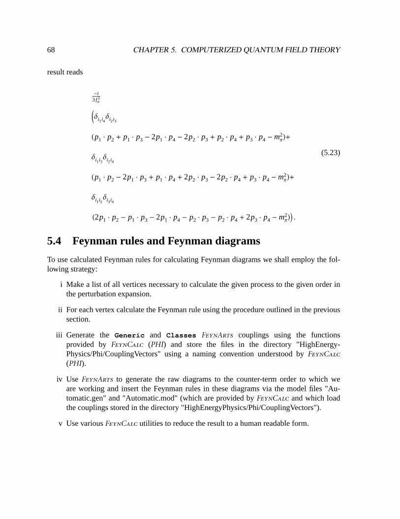
68 CHAPTER 5. COMPUTERIZED QUANTUM FIELD THEORY
result reads
-i3 f 2Π
J∆i1i4∆i2i3
(p1 × p2 + p1 × p3 - 2p1 × p4 - 2p2 × p3 + p2 × p4 + p3 × p4 -m2Π)+
∆i1i3∆i2i4
(p1 × p2 - 2p1 × p3 + p1 × p4 + 2p2 × p3 - 2p2 × p4 + p3 × p4 -m2Π)+
∆i1i2∆i3i4
(2p1 × p2 - p1 × p3 - 2p1 × p4 - p2 × p3 - p2 × p4 + 2p3 × p4 -m2Π)M .
(5.23)
5.4 Feynman rules and Feynman diagrams
To use calculated Feynman rules for calculating Feynman diagrams we shall employ the fol-lowing strategy:
i Make a list of all vertices necessary to calculate the given process to the given order inthe perturbation expansion.
ii For each vertex calculate the Feynman rule using the procedure outlined in the previoussection.
iii Generate theGeneric and Classes FeynArts couplings using the functionsprovided by FeynCalc (PHI) and store the files in the directory "HighEnergy-Physics/Phi/CouplingVectors" using a naming convention understood byFeynCalc(PHI).
iv Use FeynArts to generate the raw diagrams to the counter-term order to which weare working and insert the Feynman rules in these diagrams via the model files "Au-tomatic.gen" and "Automatic.mod" (which are provided byFeynCalc and which loadthe couplings stored in the directory "HighEnergyPhysics/Phi/CouplingVectors").
v Use variousFeynCalc utilities to reduce the result to a human readable form.

5.4. FEYNMAN RULES AND FEYNMAN DIAGRAMS 69
The first step is illustrated by the case ofΠΠ scattering inCHPT below. The second step hasbeen discussed in the previous section. In the following we shall discuss the remaining stepsone by one.
Regarding step iii: SinceFeynArts is used for the calculation of Feynman diagrams, we needto convert the vertices generated inFeynCalc notation to a form thatFeynArts understands.The standard way of doing this is to write two model definition files. One called a "generic"model definition file containing the kinematic structure for the couplings and one called a"classes" model definition file containing the isospin/particle structure. This splitting corre-sponds to the 3 different levels, "generic", "classes" and "particle", at which one can calculateamplitudes withFeynArts. These conventions are described in [Hah01]. For our purposes weneed not understand these details as we shall deal exclusively with the "classes" level. The waychosen to implement theFeynCalc® FeynArts communication is to feed the calculated ver-tices toFeynArts through the two model files "Automatic.gen" and "Automatic.mod". Thesefiles are really small programs that read settings (propagators etc.) from the activeFeynCalc(PHI) model file and couplings from the directory "HighEnergyPhysics/Phi/CouplingVectors".The coupling files in this directory have been generated with theFeynCalc (PHI) functionsMomentaCollect , GenericCoupling , ClassesCoupling andCheckF . To see how thisworks, we will again consider some examples.
Example: Storing the weakW+W+W-W- vertex
Consider the vertexmWeakfrom (5.21). First we need to tellPHI which monomials we con-sider kinematical:
$ExpansionQuantities =
Union[$ExpansionQuantities, {MetricTensor[__]}];
Then we collect these
mWeak1 = MomentaCollect[mWeak];
Next we generatemWeak1the "generic" vector by
GenericCoupling[mWeak1]
yielding (in StandardForm )
{MetricTensor[ µ1, µ4] MetricTensor[ µ2, µ3],
MetricTensor[ µ1, µ3] MetricTensor[ µ2, µ4],
MetricTensor[ µ1, µ2] MetricTensor[ µ3, µ4]}
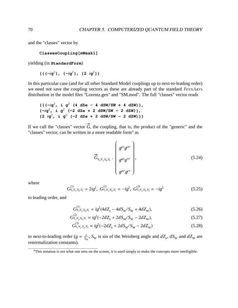
70 CHAPTER 5. COMPUTERIZED QUANTUM FIELD THEORY
and the "classes" vector by
ClassesCoupling[mWeak1]
yielding (in StandardForm )
{{(- äg2}, {- äg2}, {2 äg2}}
In this particular case (and for all other Standard Model couplings up to next-to-leading order)we need not save the coupling vectors as these are already part of the standardFeynArtsdistribution in the model files "Lorentz.gen" and "SM.mod". The full "classes" vector reads
{{(- äg2, i g 2 (4 dZe - 4 dSW/SW + 4 dZW)},
{- äg2, i g 2 (-2 dZe + 2 dSW/SW - 2 dZW)},
{2 äg2, i g 2 (-2 dZe + 2 dSW/SW - 2 dZW)}}
If we call the "classes" vector-®G, the coupling, that is, the product of the "generic" and the
"classes" vector, can be written in a more readable form4 as
-®GVi ,Vj ,Vk,Vl
.
æçççççççççççççççççççççè
gΜΝgΡΣ
gΜΡgΝΣ
gΜΣgΡΝ
ö÷÷÷÷÷÷÷÷÷÷÷÷÷÷÷÷÷÷÷÷÷ø
, (5.24)
whereG(1)Vi ,Vj ,Vk,Vl = 2ig2, G
(2)Vi ,Vj ,Vk,Vl = -ig2, G
(3)Vi ,Vj ,Vk,Vl = -ig2 (5.25)
to leading order, and
G(1)Vi ,Vj ,Vk,Vl = ig2
(4dZe- 4dSW/SW + 4dZW), (5.26)
G(2)Vi ,Vj ,Vk,Vl = ig2
(-2dZe+ 2dSW/SW - 2dZW), (5.27)
G(3)Vi ,Vj ,Vk,Vl = ig2
(-2dZe+ 2dSW/SW - 2dZW) (5.28)
to next-to-leading order (g = eSW
, SW is sin of the Weinberg angle anddZe, dSW anddZW arerenormalization constants).
4This notation is not what one sees on the screen, it is used simply to make the concepts more intelligible.

5.4. FEYNMAN RULES AND FEYNMAN DIAGRAMS 71
Example: Storing the 4-pionCHPT vertex
For renormalizable theories having a "generic" vector which contains the kinematical struc-tures is logical, since no new structures appear in the higher order counter-term lagrangians.For effective theories this is not the case. The way chosen to useFeynArts for effective the-ories is, as mentioned, through the two model files "Automatic.gen" and "Automatic.mod",which set up a "generic" vector containing all the kinematical structures (monomials) up theorder we are working. The "classes" vector then keeps track of the power counting by havingnon-zero entries only for the monomials of the given order. All this requires the environmentvariable$VerticesSpecifications to be set correctly.
Consider now the 4-pionCHPTvertex (5.23). To generate the coupling vectors to be stored,issue:
mChPT1 = MomentaCollect[mChPT1];
gChPT = GenericCoupling[mChPT1];
cChPT = ClassesCoupling[mChPT1];
These are saved in the directory "HighEnergyPhysics/Phi/CouplingVectors" by
CheckF[gChPT, XName[VertexFields ->
{Pion[0], Pion[0], Pion[0], Pion[0]},
PerturbationOrder -> 2, PhiModel -> ChPT2] <> ".Gen"];
CheckF[cChPT, XName[VertexFields ->
{Pion[0], Pion[0], Pion[0], Pion[0]},
PerturbationOrder -> 2, PhiModel -> ChPT2] <> ".Mod"];
The procedure outlined above has been carried out for manyCHPT vertices and the resultingfiles in "HighEnergyPhysics/Phi/CouplingVectors" are part of the standardFeynCalc distri-bution.
We now move on to the initially defined step iv and again consider a simple example.
Example: Møller scattering diagrams
Consider leading-order Møller scattering (see the notebook in appendixB for the full calcula-tion). First, create the topologies:
tops = CreateTopologies[0, 2 -> 2,
Adjacencies -> {3},

72 CHAPTER 5. COMPUTERIZED QUANTUM FIELD THEORY
ExcludeTopologies -> {SelfEnergies, WFCorrections},
CountertermOrder -> 0];
Insert the vertices in the topologies:
inserttops = InsertFields[tops,
Electron[0], Electron[0] -> Electron[0], Electron[0],
Model -> "Automatic", GenericModel -> "Automatic",
InsertionLevel -> Classes];
Calculate the amplitude:
amp = CreateFCAmp[inserttops]
Finally, for step v) we shall stick with the simple case of Møller scattering.
Example: Møller scattering postprocessing
The Møller cross-section can be calculated with the following code:
squaredAmp = FermionSpinSum[
(Plus @@ amp)
(ComplexConjugate[Plus @@ amp /.
{ µ1 -> ν1, µ2 -> ν1}]) /.
ParticleMass[Photon, ___] -> 0 //
Expand // Contract] /. DiracTrace -> Tr //
DiracSimplify // Contract;
squaredAmp // PropagatorDenominatorExplicit //
MandelstamReduce[#, Masses ->
ParticleMass[Electron, RenormalizationState[0]],
ParticleMass[Electron, RenormalizationState[0]],
ParticleMass[Electron, RenormalizationState[0]],
ParticleMass[Electron, RenormalizationState[0]],
MandelstamCancel -> MandelstamU] & // Simplify
The result reads
I16 I64 Im0ΨM
8- 16 (6 s- t) Im0
ΨM
6+ 4 I13s2
+ 3 t s+ 3 t2M
Im0ΨM
4- 4 I3 s3
+ 3 t s2+ 3 t2 s+ 2 t3
M Im0ΨM
2+
Is2+ t s+ t2
M
2M Ie0M
4M�It2I - 4 Im0
ΨM
2+ s+ tM
2M
(5.29)

5.4. FEYNMAN RULES AND FEYNMAN DIAGRAMS 73
Having discussed individually the steps i)-v) of a scattering amplitude calculation, we nowbriefly sketch the simple example of the calculation of the one-loop diagrams ofΠΠ scatteringin CHPT. (again, the full calculation of the one-loop scattering amplitude is contained in anotebook in appendixB).
Example: One-loop pion-pion scattering amplitude inCHPT
Create all topologies with one loop, 4- or 6-leg vertices and no self-energy or wave-functionrenormalization diagrams; tellPHI which field-vertices to use; insert these fields; create theamplitudes:
mesonstop =
CreateTopologies[1, 2 -> 2,
Adjacencies -> 4, 6,
ExcludeTopologies -> SelfEnergies, WFCorrections,
CountertermOrder -> 0];
mins = InsertFields[mesonstop,
Pion[0, i1], Pion[0, i2] ->
Pion[0, i3], Pion[0, i4],
Model -> "Automatic",
GenericModel -> "Automatic",
InsertionLevel -> Classes];
amplFC = CreateFCAmp[mins,
AmplitudeLevel -> Classes, NoSums -> True,
EqualMasses -> True];
Drawing the diagrams is done with
Paint[mins];
yielding fig.5.1The remaining contributions are calculated analogously. After adding every-thing up and simplifying using the tools provided byFeynCalc one gets the result given insection2.

74 CHAPTER 5. COMPUTERIZED QUANTUM FIELD THEORY
�
i1�
i2
�
i3�
i4
�
�
i1
�
i2
�
i3
�
i4�
�
�
i1
�
i2
�
i3
�
i4
� �
�
i1
�
i2
�
i3
�
i4
� �
Figure 5.1: One-loop diagrams of pion-pion scattering.

Conclusion
1) The calculation in Chiral Perturbation Theory of various processes, that are important forthe understanding of the strong and electro-weak forces at low energies, has been carried out.The approach has been to develop a general calculational machinery which can also be appliedto other processes. The resulting computer program has been made publicly available and canbe downloaded freely.
Two new calculations were carried out with the computer program:
• The calculation of the one-loopΠ+Π- ® Π+Π- amplitude in Chiral Perturbation Theorywith virtual photons.
• The calculation of the one-loop amplitude of K® 2Π with a momentum-carrying weakchiral lagrangian.
The conclusion from the first calculation is that electromagnetic corrections do not alter thestrong predictions by more than 5%. Therefore the extraction of the strong scattering lengthsa0
0 anda20 from theDIRAC experiment is on a sound footing. Work is under way to finish the
full radiative calculation includingO(e4) corrections. Moreover, the results of the calculation
are necessary for a complete treatment of final state interactions in K® 2Π.The second calculation allowed an order of magnitude estimate of the subtraction constant
b, needed for the analysis of final state interactions in K® 2Π.
2) Mesonic final-state interactions in K® 2Π have been analyzed. This analysis showed thatfinal state interactions do potentially resolve the discrepancy of experimental with theoreticalvalues of¶¢/¶, but that at present no conclusive statement can be made, because of the uncer-tainties due to our ignorance of the weak interaction at low energies. Our framework providesthe means of consistently including final state interactions in K® 2Π, but will remain non-predictive until the slope of the amplitude at the subtraction point has been provided e.g. by alattice calculation.
From (4.46) and fig.4.3 it is seen that the contribution of kaon loops is not of the sameorder of magnitude as the next-to-next-to-leading order contribution to the scalar form factor,but if one aims at a~ 1% level of accuracy, one should do a full coupled-channel analysis ofthe final state interactions, including the KK channel. For K® 2Π, work in this respect is alsounder way.

76 CHAPTER 5. COMPUTERIZED QUANTUM FIELD THEORY

Appendix A
PHI reference manual
This manual should serve both as a quick read for getting started with doingCHPT with Feyn-Calc and as a structured reference. It is, however, not an exhaustive reference for all functions.The full alphabetic reference can be found either with the help system coming with theFeyn-Calc distribution or on theFeynCalc web site [MO00]. Examples of applications of thesecan be found on theFeynCalc web-site [MO00].
It is assumed that the reader is familiar withMathematica, in particular with how input isgiven toMathematica and that the screen output can be chosen to be in eitherStandardForm
which can be fed back toMathematica, or in TraditionalForm which looks nice, butcannot be fed back toMathematica. The usual convention is followed: Names starting witha capital letter represent objects provided by the package (built-in).
A.1 Installing and loading the packages
TheMathematica packagePHI is distributed as a subpackage ofFeynCalc, which is avail-able at [MO00] in form of a compressed archive. InstallingFeynCalc (and therebyPHI) isdone by unpacking the archive and moving the resulting directory "HighEnergyPhysics" intoeither one of the following places:
• TheMathematica installation "Applications" directory: UnderUNIX /LINUX this wouldtypically be somewhere like "/usr/local/Mathematica/AddOns/Applications/". UnderWindows it would typically be "C:\Program Files\Wolfram Research\Mathematica\4.1\AddOns\Applications". Under MAC OS it would typically be "MacintoshHD:Applications:Wolfram Research:Mathematica:4.1:AddOns:Applications".
• Your local "Applications" directory: UnderUNIX /LINUX this is " /.Mathemat-
77

78 APPENDIX A. PHI REFERENCE MANUAL
ica/x/AddOns/Applications/", where the tilde refers to you home directory and the xto your version ofMathematica (e.g. 4.0 or 4.1; as of version 4.2 ofMathematica,"x/AddOns/" should be left out). Under other architectures there is no such directory.
In order to be able to useFeynArts together withFeynCalc, one should downloadFeynArtsfrom http://www.feynarts.de/. It should simply be extracted in the directory "HighEnergy-Physics". When done installing the packages,FeynCalc can be loaded as described below.
Before loadingFeynCalc, one should set configuration variables causingPHI and Fey-nArts to be loaded. This is done by evaluating the following:
$LoadPhi=True;$LoadFeynArts=True;
Then, the first thing to do before a calculation can be undertaken is to specify a model. Ifneeded, lagrangians to be loaded can also be specified. E.g. to specify standard SU(2)CHPT
one would have to evaluate the following before loadingFeynCalc:
$Configuration="ChPT2";$Lagrangians={"ChPT2"[2],"ChPT2"[4]};
After doing this (if often working with the same model, one may want to put the above in theconfiguration file "PhiStart.m" ), one can loadFeynCalc in the standard manner with
«"HighEnergyPhysics‘FeynCalc‘";
A.2 Framework
Consider the basic quantity inCHPT, theU(x) field containing the meson fieldsji. It is writ-ten asMM[x] . Below are shown some examples of input and the resulting screen output onevaluation
In[1]:= MM
Out[1]= U
In[2]:= ?MM

A.2. FRAMEWORK 79
MM[x] : =UFieldMatrix[QuantumField[Particle[Pion]][x]].
MM takes three optional arguments with head Renor-
malizationState, RenormalizationScheme and Expan-
sionState respectively. MM[i,x] is the i’th power of
MM[x]
In[3]:= MM[x]
Out[3]=ä®Π ×®Σ
fΠ
-
®Π ×®Σ÷®Π ×®Σ
2 ( fΠ)2 -
ä K®Π ×®Σ÷®Π ×®Σ÷®Π ×®ΣO
6 ( fΠ)3 +
®Π ×®Σ÷®Π ×®Σ÷®Π ×®Σ÷®Π ×®Σ
24 ( fΠ)4 + Id
In[4]:= MM[x, ExpansionOrder ® 6, DropOrder ® ¥]
Out[4]=ä®Π ×®Σ
fΠ
-
®Π ×®Σ÷®Π ×®Σ
2 ( fΠ)2 -
ä K®Π ×®Σ÷®Π ×®Σ÷®Π ×®ΣO
6 ( fΠ)3 +
®Π ×®Σ÷®Π ×®Σ÷®Π ×®Σ÷®Π ×®Σ
24 ( fΠ)4 +
ä K®Π ×®Σ÷®Π ×®Σ÷®Π ×®Σ÷®Π ×®Σ÷®Π ×®ΣO
120( fΠ)5 -
®Π ×®Σ÷®Π ×®Σ÷®Π ×®Σ÷®Π ×®Σ÷®Π ×®Σ÷®Π ×®Σ
720( fΠ)6 + Id
In[5]:= MM[x, ExpansionOrder ® 6, DropOrder ® 1]
Out[5]=ä À®Π ×®Σ
fΠ
+ Id
In[6]:= MM[1/2, x, ExpansionOrder ® 6, DropOrder ® 1]
Out[6]=ä À®Π ×®Σ
2 fΠ
+ Id
In[7]:= MM[1/2, x, ExpansionOrder ® 6, DropOrder ® 1]//
StandardForm
Out[7]= (ä DropFactor[PseudoScalar[2]]
IsoDot[IsoVector[QuantumField[Particle[PseudoScalar[2]]]][x],
IsoVector[UMatrix[UGenerator[]]]])/ (2 DecayConstant[PseudoScalar[2]])+
UMatrix[UIdentity]

80 APPENDIX A. PHI REFERENCE MANUAL
In[8]:= $UExpansionCoefficients
Out[8]= 91,1,12
,16
,124
,1
120,
1720
,1
5040,
140320
,1
362880,
13628800
=
These examples illustrate some general features ofMathematica:
• A function may take different numbers of arguments.
• If not supplied, optional arguments are assumed to have default values.
• The special kind of arguments called options and denoted with "®" are always optional.
• Default values for options can be set withSetOptions .
They also illustrate some general features ofFeynCalc andPHI:
• Most built-in quantities have display rules defined so that their output form is typeset(when usingTraditionalForm as output format type).
• All built-in quantities have descriptions which can be accessed in the standardMathe-matica way by using the? operator.
• The behaviour of some functions is controlled by the setting of environment variablesrecognizable by the$ as the first letter. In contrast to options, these are meant to be setonce and for all in a calculation session, preferably in the configuration "PhiStart.m" orin the chosen configuration file in the directory "Configurations". When using one of thepredefined configurations the user does not have to care about these.
A.3 Building blocks, lagrangians
As we have seen, the most important building block when constructing chiral mesonic la-grangians are theU matrix, theΧ matrix and traces and derivatives of these.
MM[x] the matrix ei
FΠϕ×σ collecting the meson
fields. Evaluating returns a result interms of dot products (IsoDot ) of isovec-tors (IsoVector ) of ϕ with isovectorsof the triplet or octet of matricesσ(UGeneratorMatrix ) generating SU(2)or SU(3)

A.3. BUILDING BLOCKS, LAGRANGIANS 81
MM[i, x] the i ’th power ofMM[x]
UChiMatrix[x] equivalent to UMatrix[UChi[]][x] .The matrix Χ containing the scalar andpseudoscalar external source fields.Depending on the setting of options,evaluating can return a result either interms of generator matrices or the uneval-uated quark mass matrix (seeUMatrix,
UGenerator, QuarkMass )
UTrace[e] attempts to calculate the trace of the ex-pressione. Only very simple expressionsare calculated; that is, terms with one sym-bolic matrix or explicitly written matri-ces. Other expressions are returned asUTrace1[e] . More complicated expres-sions can be reduced usingUExpand orWriteOutUMatrices
FieldDerivative[g[x],
x, {l1, l2, ...}]
calculates 
¶xl1
¶xl2. . . on the expression
g[x]
CovariantFieldField
Derivative[g[x], x,
{l1, l2, ...}]
as above but with the vector and axial-vector source field terms included. This isdefined in the chosen model configurationfile
Building blocks forCHPT lagrangians
These functions are predefined in terms of lower level functions, the most important of whichare listed below.
UFieldMatrix[f] matrixei
FΠf ×σ of the fieldf

82 APPENDIX A. PHI REFERENCE MANUAL
UMatrix[m] is recognized as an SU(2) or SU(3) ma-trix (depending on the setting of the op-tion GaugeGroup ). If mis one of the fourquantities below an expanded result is re-turned
UGenerator[] generic name for the matrices generatingSU(2) or SU(3)
UGenerator[i] the i ’th generating matrix
UChi[] the matrixΧ
QuarkMass[] the quark mass matrix
UQuarkCharge[] the quark charge matrix
QuantumField[f] QuantumField[f][x] represents aquantum field depending on the space-time argumentsx . QuantumField[f]
may be given as argument toIsoVector
Particle[p] represents a particle field and may be usedas the argumentf above
IsoVector[v] represents an SU(2) or SU(3) multipletwith number of entries corresponding tothe number of generators
UVector[v] represents an SU(2) or SU(3) multipletwith number of entries corresponding tothe dimension of the representation
Basic functions used internally for defining the above building blocks
ExpansionOrder the order in the meson fields to which ev-eryU matrix is expanded

A.3. BUILDING BLOCKS, LAGRANGIANS 83
DropOrder the maximal order of monomials in themeson fields (e.g. when multiplying twoU matrices)
GaugeGroup the numberN of generators of the gaugegroup SU(N)
UDimension the dimension of the representation of thegauge group
DiagonalToU whether a matrix should be written as alinear combination of the generator matri-ces and the identity matrix
QuarkToMesonMasses whether the quark masses in the quarkmass matrix should be expressed bythe meson masses using the mass re-lations $QuarkToPionMassesRules
(when GaugeGroup is set to 2) or$QuarkToMesonMassesRules (whenGaugeGroup is set to 3)
Options ofCHPT building blocks and basic functions
Adjoint[m] if m is a matrix it is adjoint, if it’s a scalar(members of$UScalars ) it’s just com-plex conjugated
Conjugate[s] complex conjugation of s. The built-infunctionConjugate has been extended toknow aboutPHI objects
Complex conjugation and adjungation
ParticleMass[p] mass of the particle p
DecayConstant[p] decay constant of the particle p

84 APPENDIX A. PHI REFERENCE MANUAL
UCouplingConstant[m, i] thei ’th coupling constant of the model m.The i is optional
RenormalizationState[i] optional argument for constants specifyingwhether or not a constant is renormalized(i =1 corresponds to the former,i =0 to thelatter)
RenormalizationOrder[i] optional argument for constants
RenormalizationScheme[i] optional argument for constants
Constants
As mentioned, not only options, but also environment variables control the behaviour ofthe defined functions and allow for customization. If for instance one wants to checkrepresentation independence (c.f. below (2.27)) one can calculate an amplitude, change$UExpansionCoefficients and verify that the result is the same as before.
$QuarkToPionMassesRules rules for translating from u, d quarkmasses to pion masses (the default is stan-dardCHPT to lowest order)
$QuarkToMesonMassesRules rules for translating from u, d, s quarkmasses to meson masses (the default isstandardCHPT to lowest order)
$UExpansionCoefficients list of coefficients used for expanding theU matrix containing the meson fields (thedefault is the exponential representation)
$UParticles list of allowed names for particle andsource fields
$ExpansionQuantities which quantities apart from powers of themomenta should be collected
$SUNBasis the basis matrices of the representation ofthe gauge group. Changing them will alsochangeSU2F, SU3F, SU3D

A.3. BUILDING BLOCKS, LAGRANGIANS 85
$ConstantIsoIndices isospin indices that are not automaticallycontracted or summed over
Environment variables controlling the behaviour ofCHPT functions
Corresponding to the way fields are grouped, there are several be multiplication operationsdefined: Single field, isovector and matrix multiplication.
NM non-commutative multiplication for matri-ces and/or fields
IsoDot dot product for isospin vectors
IsoCross cross product for isospin vectors us-ing the antisymmetric structure constantsSU2F[i,j,k] or SU3F[i,j,k]
IsoSymmetricCross cross product for isospin vectors us-ing the symmetric structure constantsSU3D[i,j,k] (0 in SU(2))
Multiplication operators for fields and field multiplets
To manipulate the expressions, a number of utility functions are provided. Which functionsshould be applied, in which order and with which options, depends on the problem underconsideration. Examples are given below.
ExpandU[e] expands IsoDot products in the expressione involving isovectors of generator matri-ces into products containing at most onegenerator matrix which can be handled byUTrace
DiscardTerms[e, Retain
® {p1 ® n1, p2 ® n2,
...}]
discards all factors of fields that do notcontainn1 particle fieldsp1, n2 particlefieldsp2, etc.

86 APPENDIX A. PHI REFERENCE MANUAL
ArgumentsSupply[e, x,
opts]
ArgumentsSupply is a function that al-lows quick entering of lagrangians. Thatis, an expressione can be given withoutheads for derivatives, Lorentz and isospinarguments and without an extra pairs ofempty brackets for scalars. The expressionis then returned with space-time argumentx and options specifications and bracketssupplied
UNMSplit[e, x , ops] returns the expressione with NMproductsof MM(without arguments) expanded in themeson fields
CycleUTraces[e] rotates factors inNMor dot products insideUTrace1 until the ’smallest’ factor is infront
CommutatorReduce[e] does some reduction on expressions con-tainingNMor dot products
NMExpand[e] distributesNMoverPlus
WriteOutIsoVectors[e] writes out isovectors (with headIsoVector ) in components
WriteOutUMatrices[e] writes out matrices (with headUMatrix )in components
IsoIndicesSupply[e] replaces dot products of isovectors withcontracted indices
SUNReduce[e] does some reduction on expressions in-volving isoindices (with headSUNIndex )
IndicesCleanup[e] renames Lorentz and isospin indices in asystematic way
Functions for manipulating lagrangians
After manipulations, the result typically contains functions of isospin indices. These have head

A.4. FEYNMAN RULES, LOOPS AND POWER COUNTING 87
SUNIndex .
SU2Delta[i,j] SU(2) Kronecker delta function
SU2F[i,j,k] SU(2) antisymmetric structure constants
SU3Delta[i,j] SU(3) Kronecker delta function
SU3F[i,j,k] SU(3) antisymmetric structure constants
SU3D[i,j,k] SU(3) symmetric structure constants
Isospin functions
As a simple example consider e.g. how the leading orderCHPT SU(3) lagrangian (2.25) wasused to derive the equations of motion (5.6) for the mesons, diagonalize the mass term andthus calculate the information (5.8) tabulated in$QuarkToMesonMassesRules . One pointof using some or all of the above functions for manipulating lagrangians is to bring it into aform where Feynman rules can simply be read off. The "reading off" can be done using thefunctionFeynRule or the lower level functionFunctionalDerivative . The task discussedin the next section is then how to generate all necessary Feynman rules (for a given process),store them and use the stored rules for doing loop Feynman diagram calculations.
A.4 Feynman rules, loops and power counting
Consider theCHPT 4-pion Feynman rule. It is derived straight-forwardly withFeynCalcas shown below (again an excerpt from aMathematica notebook with the full calculationavailable at [MO00]). Notice that the predefined lagrangianLagrangian[ChPT2[2]] ispreloaded because of the configuration choice described in the beginning of sectionA.2. It isstored in a compact notation which is expanded by the functionArgumentsSupply .
The leading order lagrangian in raw form:
In[9]:= Lagrangian [ChPT2[2]]
Out[9]=14( fΠ)2I XU÷ΧÖ\ + XΧ÷UÖ\ + YD
Μ(U)÷D
Μ(U)Ö]M
The evaluated lagrangian (external fields have been set to zero in the configuration file):

88 APPENDIX A. PHI REFERENCE MANUAL
In[10]:= ll = ArgumentsSupply [Lagrangian [ChPT2[2]], x,RenormalizationState [0], GaugeGroup ® 2,ExpansionOrder ® 4, DropOrder ® 4];
Redundant terms are discarded:In[11]:= lll = DiscardTerms [ll , Retain ® {Particle [Pion ,
RenormalizationState [0]] ® 4}, Method ® Expand ]//Simplify
Out[11]=1
48 ( fΠ)2 IY®Π ×®Σ÷®Π ×®Σ÷®Π ×®Σ÷®Π ×®Σ] (m
Π)2-
2 Y®Π ×®Σ÷®Π ×®Σ÷
ΜI
®Π M ×®Σ÷
ΜI
®Π M ×®Σ] +
Y
®Π ×®Σ÷
ΜI
®Π M ×®Σ÷®Π ×®Σ÷
ΜI
®Π M ×®Σ] +
3 Y®Π ×®Σ÷
ΜI
®Π M ×®Σ÷
ΜI
®Π M ×®Σ÷®Π ×®Σ] -
Y¶ΜI
®Π M ×®Σ÷®Π ×®Σ÷®Π ×®Σ÷
ΜI
®Π M ×®Σ] +
Y¶ΜI
®Π M ×®Σ÷®Π ×®Σ÷
ΜI
®Π M ×®Σ÷®Π ×®Σ] -
2 Y¶ΜI
®Π M ×®Σ÷
ΜI
®Π M ×®Σ÷®Π ×®Σ÷®Π ×®Σ]M
Generator matrices are traced:In[12]:= llle = ExpandU[lll , CommutatorReduce ®
True ]//Simplify
Out[12]=1
24 ( fΠ)2 KI®Π × 
ΜI
®Π MM
2+ I
ΜI
®Π M ×®Π M
2+
I
®Π ×®Π M
2(mΠ)2- 2 I®Π × ®Π÷
ΜI
®Π M × 
ΜI
®Π MM +
3 I®Π × ¶ΜI
®Π M÷
ΜI
®Π M ×®Π M -
¶ΜI
®Π M ×®Π÷®Π × 
ΜI
®Π M -
2 I¶ΜI
®Π M × 
ΜI
®Π M÷®Π ×®Π MO
Indices are supplied:
In[13]:= llll = llle //IsoIndicesSupply //IndicesCleanup //CommutatorReduce [#, FullReduce ®
True ]&//Simplify
Out[13]=(mΠ)2(Π
k1)2(Π
k2)2- 2 (Πk2
¶Τ1Π
k1- Π
k1¶Τ1Π
k2)2
24 ( fΠ)2

A.4. FEYNMAN RULES, LOOPS AND POWER COUNTING 89
Calculation of the Feynman rule:
In[14]:= melsimplified = FeynRule [llll ,{QuantumField [Particle [PhiMeson ],SUNIndex [i1 ]][p1],QuantumField [Particle [PhiMeson ],SUNIndex [i2 ]][p2],QuantumField [Particle [PhiMeson ],SUNIndex [i3 ]][p3],QuantumField [Particle [PhiMeson ],SUNIndex [i4 ]][p4]}]//Simplify
Out[14]= -1
3 ( fΠ)2 Iä I
I - (mΠ)2+ p1 × p2 + p1 × p3 - 2 p1 × p4 - 2 p2 × p3 + p2 × p4 + p3 × p4M ∆i1i4
∆i2i3+
I - (mΠ)2+ p1 × p2 - 2 p1 × p3 + p1 × p4 + p2 × p3 - 2 p2 × p4 + p3 × p4M ∆i1i3
∆i2i4-
I(mΠ)2+ 2 p1 × p2 - p1 × p3 - p1 × p4 - p2 × p3 - p2 × p4 + 2 p3 × p4M ∆i1i2
∆i3i4MM
Terms are collected according to momenta:
In[15]:= mfacoll = MomentaCollect [melsimplified ,ParticlesNumber ® 4, PerturbationOrder ® 2,ScalarproductForm ® Pair ];
Coupling vectors are generated and saved:
In[16]:= gencoup = GenericCoupling [mfacoll ];
In[17]:= classcoup = ClassesCoupling [mfacoll ];
In[18]:= CheckF[gencoup , XName[VertexFields ®
{PseudoScalar [2][0], PseudoScalar [2][0],PseudoScalar [2][0], PseudoScalar [2][0]},PerturbationOrder ® 2, PhiModel ® ChPT2] <> .Gen];
In[19]:= CheckF[classcoup , XName[VertexFields ®
{PseudoScalar [2][0], PseudoScalar [2][0],PseudoScalar [2][0], PseudoScalar [2][0]},PerturbationOrder ® 2, PhiModel ® ChPT2] <> .Mod];
The reason for collecting the monomials in the momenta is that this allows splitting in twocoupling vectors, one containing the kinematical monomials and one containing the rest. Thedot product of these two vectors then gives the full coupling. Although this splitting is of noobvious use here, this is the convention used byFeynArts (see [Hah01]). The coupling vectors

90 APPENDIX A. PHI REFERENCE MANUAL
are stored in the "Phi" subdirectory "CouplingVectors". From there they can be loaded by theFeynArts models "Automatic.gen" and "Automatic.mod".
FunctionalDerivative[
lag, {f1,...}]
where {f1,...} is of the form {Quan-tumField[name, LorentzIndex[mu], ...,SUNIndex[a]][p1],...}, calculates thefunctional derivative of lag with respect tothe field list (with incoming momenta p1,etc.) and does the fourier transform
FunctionalDerivative[
lag, {f1,...}]
where {f1,...} is of the form{QuantumField[name, LorentzIn-dex[mu],...SUNIndex[a]],...}] calculatesthe functional derivative and does partialintegration but omits the x-space deltafunctions
FeynRule[lag,{f1,...}] gives the feynmanrule corresponding tothe field configuration {f1,...} of the la-grangian lag
Functions for calculating Feynman rules. These are built-inFeynCalc functions and are describe hereonly for completeness
MomentaCollect[f] collects terms containing the variablesgiven by the setting of the optionsMomentumVariablesString andParticlesNumber

A.4. FEYNMAN RULES, LOOPS AND POWER COUNTING 91
GenericCoupling[f] constructs the kinematical coupling vec-tor to be used in a generic model filefor FeynArts from the Feynman rulef. GenericCoupling will only workon sums where each term has a mono-mial in the momenta (and other expan-sion quantities) as overall factor. Suchexpressions can usually be obtained withMomentaCollect . Also depends on thesetting of$ExpansionQuantities
ClassesCoupling[f] constructs the corresponding "Classes"coupling vector
XName[opts] generates a filename using a simple nam-ing convention
CheckF[exp,fil] If fil exists, Get s fil and returns the loadedexpressions. If fil does not exist, evaluatesexp, saves it to fil and returns the evaluatedexp. If fil ends with ".Gen" or ".Mod", thesetting ofDirectory is ignored and fil issaved in the "CouplingVectors" subdirec-tory of "Phi"
Functions for generating and saving coupling definitions
ParticlesNumber specifies the number of lines of a vertex
PerturbationOrder specifies the maximum order in themomentum and/or other pertur-bative expansion parameters from$ExpansionQuantities
ScalarProductForm specifies the scalarproduct used for themomenta

92 APPENDIX A. PHI REFERENCE MANUAL
ExtendedCollect specifies whether or not to col-lect terms containing elements from$ExpansionQuantities
Directory specifies the directory used for storingfiles
ForceSave whether or not to force evaluation and sav-ing
NoSave whether or not to save. Overrides the set-ting of ForceSave
VertexFields list of fields of a vertex
PhiModel name of the model to be used for namingfiles
XFileName name to be used for saving files. If set toAutomatic the name is generated fromthe remaining options specifications
Options of functions for generating and saving coupling definitions
Similarly to the 4-pion Feynman rule, any other Feynman rule can be generated using the pre-defined lagrangians or defining new lagrangians one self. Indeed, this has been done by theauthor, andPHI ships with a number of ready to use coupling vectors (in the directory "Cou-plingVectors"). Thus, when calculating some amplitude to some order, having all necessaryFeynman rules at our disposal, the procedure is to useFeynArts for generating all diagramsand calculating the amplitude using the models "Automatic.gen" and "Automatic.mod" in-cluded with theFeynCalc distribution [MO00]. These are actually small programs that loadthe coupling vector definitions specified by the variable$VerticesSpecifications fromthe directory "CouplingVectors" inside theFeynCalc directory hierarchy. Thus, in order to usetheFeynArts ChPT couplings distributed withFeynCalc, one must have assigned a suitablevalue to$VerticesSpecifications and give
Model -> "Automatic",GenericModel -> "Automatic"
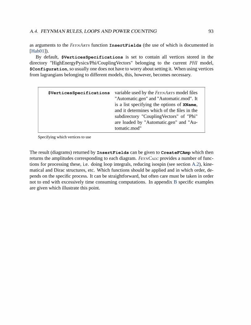
A.4. FEYNMAN RULES, LOOPS AND POWER COUNTING 93
as arguments to theFeynArts function InsertFields (the use of which is documented in[Hah01]).
By default, $VerticesSpecifications is set to contain all vertices stored in thedirectory "HighEnergyPysics/Phi/CouplingVectors" belonging to the currentPHI model,$Configuration , so usually one does not have to worry about setting it. When using verticesfrom lagrangians belonging to different models, this, however, becomes necessary.
$VerticesSpecifications variable used by theFeynArts model files"Automatic.gen" and "Automatic.mod". Itis a list specifying the options ofXName,and it determines which of the files in thesubdirectory "CouplingVectors" of "Phi"are loaded by "Automatic.gen" and "Au-tomatic.mod"
Specifying which vertices to use
The result (diagrams) returned byInsertFields can be given toCreateFCAmp which thenreturns the amplitudes corresponding to each diagram.FeynCalc provides a number of func-tions for processing these, i.e. doing loop integrals, reducing isospin (see sectionA.2), kine-matical and Dirac structures, etc. Which functions should be applied and in which order, de-pends on the specific process. It can be straightforward, but often care must be taken in ordernot to end with excessively time consuming computations. In appendixB specific examplesare given which illustrate this point.

94 APPENDIX A. PHI REFERENCE MANUAL

Appendix B
PHI applications
This chapter contains descriptions of calculations made to test the packagePHI (andFeynCalcin general andFeynArts). The calculations presented should be seen as attempts at realizingthe ideal goal set at the end of section5.1. Insofar as obtaining publication ready output fromcalculated amplitudes is by no means straightforward, the goal is not always reached and someof the notebooks do contain rather lengthy and unreadable code, mostly serving the purposeof structuring calculated expressions. Also, certainly, some of the calculations were left whena result was obtained and could use some more cleaning up. Nevertheless, in general, it is thehope that the calculations will serve the interested reader as prototypes for his own calculationswith PHI.
If you have the CD accompanying this text, the notebooks described in this chapter areavailable to you from the CD, and should run with the versions ofPHI andFeynCalc alsoon the CD. Alternatively, the notebooks can be downloaded from [Ore02]. Some of thesenotebooks will undergo improvement with time, but should run with the version ofFeynCalcavailable at the same place. Since they are compressed, they must be uncompressed beforethey can be opened withMathematica. Assuming the right versions ofPHI andFeynCalchas been installed (see sectionA.1), the notebooks should run with no further ado, as they loadFeynCalc in their preambles.
B.1 QED
These notebooks derive textbook results fromQED with one lepton, thus testing among otherthings, the handling of one-loop two-point functions with two propagators and two differentmasses in the loop, a three-point function with three propagators and two different masses, aswell as the handling of spinors.
95

96 APPENDIX B. PHI APPLICATIONS
Møller scattering
Name of file: "Moeller.nb".Available at: http://www.feyncalc.org/phi/examples/QED/Moeller.nb.gz.Description: The Møller differential cross section to leading order.
Radiative corrections
Name of file: "QEDRadiativeCorrections.nb".Available at: http://www.feyncalc.org/phi/examples/QED/QEDRadiativeCorrections.nb.gz.Description: The photon self-energy, the electron self-energy and the photon-electron-electron vertex correction to one loop inQED.
B.2 CHPT, pions
These notebooks derive some of the classical SU(2) results of Gasser and Leutwyler [GL84]using Feynman diagram techniques for the calculation of amplitudes.
Lagrangians
Name of file: "EOMTricks.nb".Available at:http://www.feyncalc.org/phi/examples/ChPT/Pions/EOMTricks.nb.gz.Description: Useful SU(2) equation of motion relations are derived.
Name of file: "GeneratingFunctional.nb".Available at:http://www.feyncalc.org/phi/examples/ChPT/Pions/GeneratingFunctional.nb.gz.Description: The one-loop generating functional is derived.
Feynman rules
Name of file: "FeynmanRules.nb".Available at:http://www.feyncalc.org/phi/examples/ChPT/Pions/FeynmanRules.nb.gz.Description: The pionicO(p2
) 4,6-vertices and theO(p2) 4-vertex are calculated and stored.
Name of file: "PSFeynmanRules.nb".

B.2. CHPT, PIONS 97
Description: Pionic vertices with external pseudo-scalar and scalar fields are calculated andstored.Available at:http://www.feyncalc.org/phi/examples/ChPT/Pions/PSFeynmanRules.nb.gz.
Two-point amplitudes
Name of file: "WaveFunctionFactor.nb".Available at:http://www.feyncalc.org/phi/examples/ChPT/Pions/WaveFunctionFactor.nb.gz.Description: The one-loop pion wave-function and mass renormalization factors are calcu-lated and stored.
Name of file: "DecayConstantFactor.nb".Available at:http://www.feyncalc.org/phi/examples/ChPT/Pions/DecayConstantFactor.nb.gz.Description: The one-loop renormalization of the pion decay constant is calculated and stored.
Name of file: "PionPseudoscalarFactor.nb".Available at:http://www.feyncalc.org/phi/examples/ChPT/Pions/PionPseudoscalarFactor.nb.gz.Description: The two-point pion-pseudo-scalar correlator to one loop is calculated and stored.
Scalar form factor
Name of file: "ScalarFormFactor.nb".Available at:http://www.feyncalc.org/phi/examples/ChPT/Pions/ScalarFormFactor.nb.gz.Description: The pion scalar form factor to one loop.
Pion-pion scattering
Name of file: "PiPiScattering.nb".Available at:http://www.feyncalc.org/phi/examples/ChPT/Pions/PiPiScattering.nb.gz.Description: The one-loop pion-pion scattering amplitude. Partial wave and isospin projec-tions are given.

98 APPENDIX B. PHI APPLICATIONS
B.3 CHPT, pions and photons
Amplitudes involving the external vector field of the covariant derivative are calculated.
Feynman rules
Name of file: "FeynmanRules.nb".Description: Pionic vertices with an external vector field are calculated and stored.Available at:http://www.feyncalc.org/phi/examples/ChPT/Pions+Photons/FeynmanRules.nb.gz.
Vector form factor
Name of file: "PhotonFormFactor.nb".Available at:http://www.feyncalc.org/phi/examples/ChPT/Pions+Photons/PhotonFormFactor.nb.gz.Description: The vector form factor to one loop.
Compton scattering
Name of file: "ComptonScattering.nb".Available at:http://www.feyncalc.org/phi/examples/ChPT/Pions+Photons/ComptonScattering.nb.gz.Description: Compton scattering of a pion and an external vector field to one loop.
B.4 CHPT, mesons
These notebooks derive some of the classical SU(3) results of [GL85] as well as a few 3- and4-point amplitudes.
Lagrangians
Name of file: "EquationsOfMotion.nb".Available at:http://www.feyncalc.org/phi/examples/ChPT/Mesons/EquationsOfMotion.nb.gz.Description: The SU(3) equations of motion are derived.
Name of file: "EOMTricks.nb".

B.4. CHPT, MESONS 99
Available at:http://www.feyncalc.org/phi/examples/ChPT/Mesons/EOMTricks.nb.gz.Description: Useful SU(2) equation of motion relations are derived.
Name of file: "GeneratingFunctional.nb".Available at:http://www.feyncalc.org/phi/examples/ChPT/Mesons/GeneratingFunctional.nb.gz.Description: The one-loop generating functional is derived.
Feynman rules
Name of file: "FeynmanRules.nb".Available at:http://www.feyncalc.org/phi/examples/ChPT/Mesons/FeynmanRules.nb.gz.Description: The mesonic SU(3)O(p2
) 4,6-vertices and theO(p2) 4-vertex are calculated and
stored.
Name of file: "SFeynmanRules.nb".Available at:http://www.feyncalc.org/phi/examples/ChPT/Mesons/PSFeynmanRules.nb.gz.Description: Mesonic SU(3) vertices with an external scalar field are calculated and stored.
Two-point amplitudes
Name of file: "WaveFunctionFactor.nb".Available at:http://www.feyncalc.org/phi/examples/ChPT/Mesons/WaveFunctionFactor.nb.gz.Description: The one-loop meson SU(3) wave-function and mass renormalization factors arecalculated and stored.
Name of file: "DecayConstantFactor.nb".Available at:http://www.feyncalc.org/phi/examples/ChPT/Mesons/DecayConstantFactor.nb.gz.Description: The one-loop renormalization of the pion, kaon and eta-meson decay constantsare calculated and stored.
Name of file: "MesonPseudoscalarFactor.nb".Available at:http://www.feyncalc.org/phi/examples/ChPT/Mesons/MesonPseudoscalarFactor.nb.gz.Description: The two-point one-loop correlators of a pseudo-scalar external field with a pion,kaon and an eta-meson are calculated and stored.

100 APPENDIX B. PHI APPLICATIONS
Scalar form factor
Name of file: "ScalarFormFactor.nb".Available at:http://www.feyncalc.org/phi/examples/ChPT/Mesons/ScalarFormFactor.nb.gz.Description: The SU(3) meson scalar form factors to one loop.
Meson-meson scattering
Name of file: "MesonMesonScattering-pions.nb".Available at:http://www.feyncalc.org/phi/examples/ChPT/Pions/MesonMesonScattering-pions.nb.gz.Description: The one-loop SU(3) pion-pion scattering amplitudes.Name of file: "MesonMesonScattering-kaons.nb".Available at:http://www.feyncalc.org/phi/examples/ChPT/Pions/MesonMesonScattering-kaons.nb.gz.Description: The one-loop kaon-kaon scattering amplitudes.
B.5 CHPT, pions and virtual photons
Following [KU98], the EM interaction is incorporated through the inclusion of virtual photonsin the lagrangians. The one-loop generating functional is explicitly calculated, making useof the Cayley-Hamilton equations of motion. Also, the amplitude given in appendixC.1.1iscalculated.
Lagrangians
Name of file: "EquationsOfMotion.nb".Available at:http://www.feyncalc.org/phi/examples/ChPT/Pions+VirtualPhotons/EquationsOfMotion.nb.gz.Description: The SU(2) equations of motion for the pion and the photon are derived.
Name of file: "EOMTricks.nb".Available at:http://www.feyncalc.org/phi/examples/ChPT/Pions+VirtualPhotons/EOMTricks.nb.gz.Description: Useful equation of motion relations are derived.

B.5. CHPT, PIONS AND VIRTUAL PHOTONS 101
Name of file: "GeneratingFunctional.nb".Available at:http://www.feyncalc.org/phi/examples/ChPT/Pions+VirtualPhotons/GeneratingFunctional.nb.gz.Description: The one-loop generating functional with virtual photons is derived.
Feynman rules
Name of file: "FeynmanRules.nb".Available at:http://www.feyncalc.org/phi/examples/ChPT/Pions+VirtualPhotons/FeynmanRules.nb.gz.Description: Feynman rules with virtual photons are calculated and stored.
Two-point amplitudes
Name of file: "WaveFunctionFactor.nb".Available at:http://www.feyncalc.org/phi/examples/ChPT/Pions+VirtualPhotons/WaveFunctionFactor.nb.gz.Description: The one-loop pion wave-function and mass renormalization factors are calcu-lated and stored.
Name of file: "PhotonWaveFunctionFactor.nb".Available at:http://www.feyncalc.org/phi/examples/ChPT/Pions+VirtualPhotons/PhotonWaveFunctionFactor.nb.gz.Description: The one-loop photon wave-function renormalization factor is calculated andstored.
Name of file: "DecayConstantFactor.nb".Available at:http://www.feyncalc.org/phi/examples/ChPT/Pions+VirtualPhotons/DecayConstantFactor.nb.gz.Description: The one-loop renormalization of the pion decay constant with virtual photons iscalculated and stored.
102 APPENDIX B. PHI APPLICATIONS
Pion pion scattering
Name of file: "PiPiScattering.nb".Available at:http://www.feyncalc.org/phi/examples/ChPT/Pions+VirtualPhotons/PiPiScattering.nb.gz.Description: The one-loop pion-pion scattering amplitude with virtual photons. All channelscan be calculated.O(e4
) contributions are also calculated.
B.6 Weak CHPT
TheDS= 1 lagrangians of [EKW93] are coupled to an external source and used for calculatingthe amplitudes used given in sectionC.2.
Feynman rules
Name of file: "FeynmanRules.nb".Available at:http://www.feyncalc.org/phi/examples/ChPT/Weak/FeynmanRules.nb.gz.Description: Feynman rules of mesons and an axial external field using the weak lagrangianare calculated and stored.
Name of file: "SFeynmanRulesA.nb".Available at:http://www.feyncalc.org/phi/examples/ChPT/Weak/SFeynmanRulesA.nb.gz.Description: O(p2
) Feynman rules of mesons and the weak lagrangian lagrangian are calcu-lated and stored.
Name of file: "SFeynmanRulesB.nb".Available at:http://www.feyncalc.org/phi/examples/ChPT/Weak/SFeynmanRulesB.nb.gz.Description: O(p4
) Feynman rules of mesons and the weak lagrangian lagrangian are calcu-lated and stored.
Name of file: "PFeynmanRules.nb".Available at:http://www.feyncalc.org/phi/examples/ChPT/Weak/PFeynmanRules.nb.gz.Description: Feynman rules of mesons, a pseudo-scalar external field and the weak lagrangianare calculated and stored.

B.6. WEAK CHPT 103
Name of file: "S2FeynmanRules.nb".Available at:http://www.feyncalc.org/phi/examples/ChPT/Weak/S2FeynmanRules.nb.gz.Description: Feynman rules of mesons, a scalar external field and the weak lagrangian arecalculated and stored.
Two-point amplitudes
Name of file: "ScalarMesonFactor.nb".Available at:http://www.feyncalc.org/phi/examples/ChPT/Weak/ScalarMesonFactor.nb.gz.Description: The two-point one-loop correlators of a scalar external field with a kaon arecalculated and stored.
K ® Π
Name of file: "KSPiAmplitude.nb".Available at:http://www.feyncalc.org/phi/examples/ChPT/Weak/KSPiAmplitude.nb.gz.Description: The three-point function of a kaon, a pion and the weak lagrangian.
Name of file: "KSPiChecks.nb".Available at:http://www.feyncalc.org/phi/examples/ChPT/Weak/KSPiChecks.nb.gz.Description: Various checks and reduction of the expressions of "KSPiAmplitude.nb".
K ® 2Π
Name of file: "A7PiPiAmplitude.nb".Available at:http://www.feyncalc.org/phi/examples/ChPT/Weak/A7PiPiAmplitude.nb.gz.Description: The one-loop three-point function of an external axial-vector field with the SU(3)index of Ks and two neutral pions.
Name of file: "P7PiPiAmplitude.nb".Available at:http://www.feyncalc.org/phi/examples/ChPT/Weak/P7PiPiAmplitude.nb.gz.Description: The leading order three-point function of an external pseudo-scalar field withthe SU(3) index of Ks and two neutral pions.

104 APPENDIX B. PHI APPLICATIONS
Name of file: "KSPiPiAmplitude.nb".Available at:http://www.feyncalc.org/phi/examples/ChPT/Weak/KSPiPiAmplitude.nb.gz.Description: The four-point function of a Ks, two neutral pions and the weak lagrangian.
Name of file: "KSPiPiChecksA.nb".Available at:http://www.feyncalc.org/phi/examples/ChPT/Weak/KSPiPiChecksA.nb.gz.Description: Various checks of the expressions of "KSPiPiAmplitude.nb".
Name of file: "KSPiPiChecksB.nb".Available at:http://www.feyncalc.org/phi/examples/ChPT/Weak/KSPiPiChecksB.nb.gz.Description: Reduction of the expressions of "KSPiPiAmplitude.nb".
K ® s
Name of file: "KSS2Amplitude.nb.nb".Available at:http://www.feyncalc.org/phi/examples/ChPT/Weak/KSS2Amplitude.nb.nb.gz.Description: The three-point function of a kaon, an external scalar field and the weak la-grangian.
Name of file: "KSS2Checks.nb.nb".Available at:http://www.feyncalc.org/phi/examples/ChPT/Weak/KSS2Checks.nb.nb.gz.Description: Various checks and reduction of the expressions of "KSS2Amplitude.nb".

Appendix C
One-loop amplitudes
C.1 Pion-pion scattering
C.1.1 Π+Π-® Π
+Π-
Leading order:
T (2) =1
f 2 (-2m2Π
0 + s+ t)+ (C.1)
1
f 2st9-2e2 f 2
Is2+ st+ t2
- 2m2Π+(s+ t)M= .
Rational contribution from the loops:
T(4)
poly = -4e4
288Π2st(s- 4m2Π+)(t - 4m2
Π+)
(C.2)
(-9344m8Π+ + 8m4
Π+(73s2
+ st+ 73t2)+
st(109s2+ 199st+ 109t2
)+
2336m6Π+u+ 2m2
Π+u(146s2
+ 543st+ 146t2))-
1
288f 4Π
2
105

106 APPENDIX C. ONE-LOOP AMPLITUDES
(280m4Π+ + 198m4
Π0 + 23s2
+ 20st+ 23t2+
90m2Π
0u- 2m2Π+(324m2
Π0 + 17u))-
4e2
288f 2Π
2(s- 4m2
Π+)(t - 4m2
Π+)
(54m2Π
0(-4m2Π+ + s)(4m2
Π+ - t) - 69stu-
4m2Π+(51s2
+ 91st+ 51t2+ 292m2
Π+u- 816m4
Π+)).
Counter-terms:
T(4)
CT =2e2
9 f 2 A4(-10k1 - 10k2 + 18k3 + 9k4 + 9l6)m2Π++ (C.3)
2(10k1 + 10k2 + 9(2k3 - k4 + 8(k6 + k8)))m2Π
0-
(-10k1 + 26k2 + 54k3 + 27k4 + 27l6)uE+
1
f 4 A4l3m4Π
0 + 2l1(-8m4Π+ + s2
+ t2+ 4m2
Π+u)+
l2(-32m4Π+ + 3s2
+ 4st+ 3t2+ 12m2
Π+u)E+
8e4
9A10h2 + 18k14- 5k15+
5st((2h2 - k15)(-8m4
Π+ + s2
+ t2+ 2m2
Π+u)-
l5(-8m4Π+ + s2
+ st+ t2+ 2m2
Π+u))E.
Logs:
T(4)
log = -e4 log(m2
Γ/Μ2)
2Π2 - (C.4)

C.1. PION-PION SCATTERING 107
log(m2Π+/Μ2)
96f 4Π
2 A8e2 f 2(8m2
Π+ - 9m2
Π0 + 3u)+
4e4 f 4
st(-8m4
Π+ + s2
+ 7st+ t2+ 2m2
Π+u)+
(64m4Π+ + 60m4
Π0 + 5s2
+ 8st+ 5t2+
24m2Π
0u- 4m2Π+(48m2
Π0 + u))E-
log(m2Π
0/Μ2)
32f 4Π
2 A10m4Π
0 + s2+ t2+ 4m2
Π0(u- 4m2
Π+)E.
J’s (see appendixC.4):
T(4)
J = Jm2Γ,m2Γ
(s)4e4+ Jm2
Γ,m2Γ
(t)4e4+ (C.5)
Jm2Π0,m2Π0(s)
2 f 4 (-m2Π
0 + s)2 +Jm2Π0,m2Π0(t)
2 f 4 (-m2Π
0 + t)2+
Jm2Π+ ,m2
Π+(u)
2 f 4 (-2e2 f 2- 4m2
Π+ + 2m2
Π0 + u)2+
Jm2Π+ ,m2
Π+(s)
6 f 4s2(s- 4m2
Π+)
As2(s- 4m2
Π+)(4(6m4
Π0 - 3m2
Π0(4m2
Π+ + s)+
m2Π+(8m2
Π+ + 2s- t)) + s(2s+ t))+
4e2 f 2s(32m6Π+ + s2
(6m2Π
0 - 8s- 13t)-
16m4Π+(3s+ t) + 2m2
Π+s(-12m2
Π0 + 21s+ 16t))+
4e4 f 4(-32m
6Π+ - 28m2
Π+s(3s+ 2t)+
8m4Π+(15s+ 2t) + s2
(14s+ 25t))E + (sW t)

108 APPENDIX C. ONE-LOOP AMPLITUDES
Jm2Π+ ,m2
Γ
(m2Π+)
3 f 2(s- 4m2
Π+)(t - 4m2
Π+)
4e2
A - 8m2Π+st+ 6m2
Π0(s- 4m2
Π+)(t - 4m2
Π+)-
80m4Π+u+ 3stu+ 6e2 f 2
(-16m4Π+ + s2
+ st+ t2+ 8m2
Π+u)E.
C0’s (see sectionC.4):
T(4)
C0 =e4
2Π2C0(s, m2Π+, m2
Π+, m2
Γ, m2Γ, m2Π+)(s- 2m2
Π+)+ (C.6)
e4
2Π2C0(t, m2Π+, m2
Π+, m2
Γ, m2Γ, m2Π+)(t - 2m2
Π+)+
1
16C f2Π
2sC0(s, m2
Π+, m2
Π+, m2
Π+, m2
Π+, m2
Γ)
(s- 2m2Π+)( f 2(-4m4
Π+ + 7m2
Π+m
2Π
0 - 3m4Π
0)s+
2Ce2(4e2 f 2
(s+ t - 2m2Π+) + s(2u- 4m2
Π+ +m2
Π0)))+
1
16C f2Π
2tC0(t, m2
Π+, m2
Π+, m2
Π+, m2
Π+, m2
Γ)
(t - 2m2Π+)( f 2(-4m4
Π+ + 7m2
Π+m
2Π
0 - 3m4Π
0)t+
2Ce2(4e2 f 2
(-2m2Π+ + s+ t) + t(-4m2
Π+ +m2
Π0 + 2u)))-
1
16C f2Π
2C0(u, m2Π+, m2
Π+, m2
Π+, m2
Π+, m2
Γ)
(u- 2m2Π+)( f 2(-4m4
Π+ + 7m2
Π+m
2Π
0 - 3m4Π
0)+
2Ce2(-4e2 f 2
- 4m2Π+ +m2
Π0 + 2u)).
D0’s (see appendixC.4):

C.2. NON-LEPTONIC KAON DECAYS 109
T(4)
D0 =e4
4Π2 I (C.7)
D0(s, m2Π+, t, m2
Π+, m2
Π+, m2
Π+, m2
Γ, m2Γ, m2Π+, m2
Π+)(t - 2m2
Π+)
2+
D0(s, m2Π+, t, m2
Π+, m2
Π+, m2
Π+, m2
Π+, m2
Π+, m2
Γ, m2Γ)(s- 2m2
Π+)
2+
D0(s, m2Π+, u, m2
Π+, m2
Π+, m2
Π+, m2
Γ, m2Γ, m2Π+, m2
Π+)(u- 2m2
Π+)
2+
D0(t, m2Π+, u, m2
Π+, m2
Π+, m2
Π+, m2
Γ, m2Γ, m2Π+, m2
Π+)(u- 2m2
Π+)
2M.
Notice that any of the other (4 independent) elastic scattering processes involvingΠ+,Π and/or
pi0 can easily be calculated with the notebook described in appendixB. Therefore the expres-sions are not given here.
C.2 Non-leptonic kaon decays
The expressions given in this section use the counter-term basis of ref. [EKW93]. They reduceto the off-shell expressions with a static lagrangian given in ref. [KMW91] and in [BPP98], ifone translates into theEi counter-term basis used by these authors. Notice that there is a signerror onE3 andE4 in the translation table (2.19) of [BPP98].
C.2.1 K l ® Π0
Leading order:
X(2)= 4B2
0((2c5 - c2)m2K - c2m
2Π+ c2q
2). (C.8)
Logs:
X(4)log =
B20
288f 2Π
2(m2Π-m2
K)(C.9)
Alog(m2Π/Μ2)

110 APPENDIX C. ONE-LOOP AMPLITUDES
9m2Π(3m2
Π- 7m2
K + 5q2)((c2 - 2c5)m
2K + c2m
2Π- c2q
2)+
log(m2K/Μ2)
18m2K 9(m
2Π-m2
K)((11c2 - 10c5)m2K + 7c2m
2Π)+
(2(3c2 + c5)m2K - 8c2m
2Π)q2+ c2q
4=+
log(m2Η/Μ2)
3m2Η9(10c5 - 9c2)m
4K + 2(14c2 - 17c5)m
2Km2Π+ 5c2m
4Π
-2((8c2 - 9c5)m2K + 7c2m
2Π)q2+ 9c2q
4=E .
Loop functions (see appendixC.4):
X(4)JK =
B20
18f 2 (C.10)
BJmKmΗ
(q2)
9(11c2 - 12c5)m4K + 6(3c2 - 2c5)m
2Km2Π- 5c2m
4Π-
3(3(3c2 - 2c5)m2K + c2m
2Π)q2+ 9c2q
4=+
JmΠmK(q2)
9 9-(c2 + 4c5)m4K + 2(5c2 - 2c5)m
2Km2Π- c2m
4Π+
((-7c2 + 10c5)m2K - 7c2m
2Π)q2+ 5c2q
4=+
(m2Π-m2
K)
6:-KmKmΗ
(q2)((6c5 - 7c2+)m
2K + c2m
2Π)+
C.2. NON-LEPTONIC KAON DECAYS 111
9KmΠmK(q2)((c2 - 2c5)m
2K + c2m
2Π)>F .
Strong counter-terms:
X(4)Li = -
64B20
f 2 (C.11)
((c2 - 2c5)m2K + c2m
2Π- c2q
2)(m2
Π(2L6 + L8) +m2
K(4L6 + L8)).
Weak counter-terms contributing also to K® Π with q = 0:
X(4)N5,8,10,11 =
c2B20
f 28(C.12)
9-m4ΠN8 + q2
(m2ΠN8 + 2m2
K(N5 + N8))
-2m4K(N5 + N8 - 2(N10+ N11))
+m2Km2Π(-2N5 - 3N8 + 2N11+ 4N12)= .
Weak counter-terms not contributing to K® Π with q = 0:
X(4)N20-23 =
4c2B20
f 2 (C.13)
92q4N20- (m2Π-m2
K)2(2N21+ N22+ 2N23)
+q2(m2
K(-2N20- 2N21+ N22+ 2N23)
+m2Π(-2N20+ 2N21+ N22+ 2N23))= .

112 APPENDIX C. ONE-LOOP AMPLITUDES
C.2.2 Ks® 2Π0
Leading order:
T+(2) =i
2 f 2 9c2 (-m2K + 4m2
Π+ q2- 3s)+ (C.14)
1
q2-m2
K
I2c5 (m2K -m2
Π)(-m2
K + q2+ s)M? .
Logs:
T+(4)
log,tu =i
Π2 f 4(m2
K -m2Π)(q2-m2
K)(C.15)
Clog(m2Η/Μ2)
m2Η
256
9((7c2 - 6c5)m2K + 6c5m
2Π)t2+
2((5c2 + 6c5)m2K - 6c5m
2Π)tu+
((7c2 - 6c5)m2K + 6c5m
2Π)u2-
c2q2(7t2+ 10tu+ 7u2
)=+
log(m2K/Μ2)m2
K
192
9((5c2 - 18c5)m2K + 18c5m
2Π)t2+
2((c2 - 12c5)m2K + 12c5m
2Π)tu+
((5c2 - 18c5)m2K + 18c5m
2Π)u2-
c2q2(5t2+ 2tu+ 5u2
)=-
log(m2Π/Μ2)
m2Π
768

C.2. NON-LEPTONIC KAON DECAYS 113
9-((49c2 + 102c5)m2K - 102c5m
2Π)t2-
2((71c2 + 42c5)m2K - 42c5m
2Π)tu-
((49c2 + 102c5)m2K - 102c5m
2Π)u2+
c2q2(49t2
+ 142tu+ 49u2)=G.
T+(4)
log,s =-i
6912f 4(m2
K -m2Π)
(C.16)
Clog(m2Η/Μ2)
1
Π2(q2-m2
K)2
98c5(-m2K +m2
Π) I2m4
Πq2(-2q2
+ 15s)-
m6K(-45m2
Π- 100q2
+ 108s)-
m2Km2Π(-50q4
+ 36m2Πs+ 5q2
(m2Π+ 12s))
+m4K(9m4
Π+ 5m2
Π(-19q2
+ 18s) + 4q2(-25q2
+ 21s))M-
12c2(-m2K + q2
) I-64m8K +m2
K(9m6Π+
m4Π(22q2
- 9s) + 3m2Πq2(8q2- 7s)+
12q4(q2- s)) + 3m2
Πq4(-q2
+ s) -m6Π(9q2+ s)+
6m4Πq2(-2q2
+ 3s) +m6K(-97m2
Π- 8q2
+ 124s)-
2m4K(5m4
Π- 30q4
+ 3m2Πs+ q2
(-38m2Π+ 48s))M=+
log(m2K/Μ2)
18
Π2(m2
K - q2)

114 APPENDIX C. ONE-LOOP AMPLITUDES
9-6c5(-m2K +m2
Π) I15m6
K + 3m2Πs(q2+ s)-
m4K(-18m2
Π- 8q2
+ 23s)-
m2K(-16m4
Π- 5q4
+ 11q2s+ 9m2Π(-2q2
+ s))M+
c2 I-23m8K + 3m2
Πq2s(-q2
+ 3s)-
m6K(-158m2
Π- 57q2
+ 137s)+
m4K(-156m4
Π- 41q4
+ 143m2Πs+ q2
(-220m2Π+ 162s))-
m2K(-7q6
+ 9m2Πs2+ q4(-62m2
Π+ 13s)+
4q2(-39m4
Π+ 38m2
Πs))M=+
log(m2Π/Μ2)
36
Π2(m2
K - q2)
96c5(-m2K +m2
Π) I12m6
Π+m2
Πq2(3q2- 7s)+
2m4Π(4q2- 7s) + 2m4
K(m2Π- s)+
m2K(13m4
Π-m2
Π(-6q2
+ s) + 2s(q2+ s))M+
c2 I3m6Π(25q2
+ 3s) -m6K(17m2
Π+ 6s)-
4m2Πq4(-4q2
+ 7s) - 2m4Πq2(-34q2
+ 19s)-
m4K(46m4
Π- 64m2
Πs+ 18s2
- 3q2(-3m2
Π+ 4s))+
m2K(-75m6
Π+ q4(10m2
Π- 6s) + 29m4
Πs+
q2(-22m4
Π- 36m2
Πs+ 18s2
))M=+

C.2. NON-LEPTONIC KAON DECAYS 115
288
q2-m2
K
9k(m2K, m2
Η)(-m2
K +m2Π)2(-m2
Π+ q2)
(5c2 + (6c5(-m2K +m2
Π)))+
k(m2Π, m2
K)(-m2K +m2
Π)2(-m2
Π+ q2)
(c2 + (6c5(-m2K +m2
Π)))=G
Loop functions (see appendixC.4):
T+(4)
JKMr,c2=
i c2
864f 4 (C.17)
CJm2Η,m2Η
(s) 24m2Π(-13m2
K + 4m2Π- 3q2
+ 9s)+
Jm2K ,m2
K(s) 108s(-3m2
K - q2+ 3s)-
Jm2Π,m2Π
(s) 216(-m2Π+ 2s)(m2
K - 4m2Π- q2+ 3s)+
Jm2K ,m2
Η
(t)
(302m4K - 3q2
(-91m2K + 19m2
Π+ 24t)+
m2K(443m2
Π- 480t - 420u)-
m2Π(97m2
Π+ 24t - 60u) + 18t(7t + 5u))+
Jm2Π,m2
K(t)
9(-42m4K - 13m4
Π+

116 APPENDIX C. ONE-LOOP AMPLITUDES
q2(-19m2
K + 35m2Π- 16t)-
4m2Π(16t + u) + 2t(23t + u)+
m2K(103m2
Π- 4(6t + u)))+
Km2K ,m2
Η
(t)
12(-26m4K +m2
K(31m2Π+ 13q2
- 5u)+
m2Π(17q2
+ 5(-7m2Π+ u)))+
Km2Π,m2
K(t)
36(-10m4K +m2
Π(17m2
Π- 11q2
+ u)-
m2K(-23m2
Π+ 19q2
+ u))+
Mrm2
K ,m2Η(t) 540(-m2
K +m2Π)(-m2
Π+ q2)+
Mrm2Π,m2
K(t) 108(-m2
K +m2Π)(-m2
Π+ q2)+
(t W u)G.
T(4)
JKMr,c5=
i c5(m2K -m2
Π)
144f 4(q2-m2
K)(C.18)
CJm2Η,m2Η
(s) 8m2Π(q2+ 9(-m2
K + s))+
Jm2K ,m2
K(s) 108s(-m2
K + q2+ s)+
Jm2Π,m2Π
(s) 72(-m2K + q2
+ s)(-m2Π+ 2s)+

C.2. NON-LEPTONIC KAON DECAYS 117
Jm2K ,m2
Η
(t)
(-46m4K + 5m4
Π+ 21m2
Πq2- 24m2
Πt+
18t2- 12m2
Πu- 18tu+
m2K(-31m2
Π- 45q2
+ 24t + 84u))+
Jm2Π,m2
K(t)
9(-6m4K + q2
(3m2K + 13m2
Π- 8t)-
m2Π(3m2
Π+ 24t - 4u)+
2t(9t - u) +m2K(25m2
Π- 16t + 4u))+
Km2K ,m2
Η
(t)
(-12)(2m4K -m2
K(m2Π- 5q2
+ u)+
m2Π(-7m2
Π+ q2+ u))-
Km2Π,m2
K(t)
36((m2K +m2
Π)(2m2
K - 3m2Π+ q2)+
(-m2K +m2
Π)u)-
Mrm2
K ,m2Η(t) 108(-m2
K +m2Π)(-m2
Π+ q2)-
Mrm2Π,m2
K(t) 108(-m2
K +m2Π)(-m2
Π+ q2)+
(t W u)G.

118 APPENDIX C. ONE-LOOP AMPLITUDES
(C.19)
Rational contribution from the loops:
T+(4)
pol =i
1152f 4Π
2 (C.20)
C
2c5(m2K -m2
Π)
(q2-m2
K)(66q4
+ q2(147m2
K + 283m2Π- 192s)-
3(-27m4K - 90m4
Π+ 89m2
Πs+
m2K(-99m2
Π+ 37s) + 46tu+ 22(t2
+ u2)))+
c2(-103m4K - 84q4
+ 5m2K(-73m2
Π+ 57s)+
q2(-187m2
K - 311m2Π+ 138s)+
3(-90m4Π+ 37m2
Πs+ 58tu+ 28(t2
+ u2)))G.
Strong counter-terms:
T+(4)
Li =c54i(m2
Π-m2
K)
3 f 4(q2-m2
K)2 (C.21)
Cq4;-2(12L2 + 3L3 + 4L4 + 2L5 - 8L6 - 4L8)m
2K-
2(24L1 + 12L2 + 9L3 - 10L4 - 4L6 - 6L8)m2Π+
3(8L1 + 4L2 + 3L3)s?+
3m2K;(-((8L1 + 4L2 + 3L3-

C.2. NON-LEPTONIC KAON DECAYS 119
12L4 - 2L5 + 8L6 + 4L8)m2K)-
2(8L1 + 4L2 + 3L3 - 5L4+ (C.22)
2(-L5 + L6 + L8))m2Π)s+
(8L1 + 4L2 + 3L3)s2+
2(-((2L4 + L5 - 4L6 - 2L8)m4K)+
(8L1 + 4L2 + 3L3 - 13L4-
4L5 + 18L6 + 10L8)m2Km2Π+
(4L2 + L3)m4Π- (4L2 + L3)tu)?+
q2;6(-2(4L4 + L5 - 4L6 - 2L8)m
2K+
(8L1 + 4L2 + 3L3 - 6L4 - 2L5 + 4L6 + 2L8)m2Π)s-
3(8L1 + 4L2 + 3L3)s2+
2((12L2 + 3L3 + 5(2L4 + L5 - 4L6 - 2L8))m4K+
(29L4 + 12L5 - 58L6 - 36L8)m2Km2Π-
3(4L2 + L3)m4Π+ 3(4L2 + L3)tu)?G.
Weak counter-terms contributing also to K® Π with q = 0:
T+(4)
N5,8,10,11 =-ic2
3 f 4 (C.23)

120 APPENDIX C. ONE-LOOP AMPLITUDES
C2(-m2K +m2
Π)(m2
ΠN11+ 2m2
K(N10+ N11))
(m2K - q2
+ 3s)/ (q2-m2
K)-
3{(-2m4K(-8(N10+ N11) + 3N5 + 3N8))/3+ 2m2
K(N5 + N8)q2+
(4m4Π(-6N10- 14N11- 6N12+ 6N5 + 12N7 + 3N8))/3+
m2Π((m2
K(8(N10+ 5N11+ 3N12) - 48N7 + 21N8 + 18N9))/3+
(N8 + 2N9)q2) - 2(m2
K + 2m2Π)(N5 - 4N7 + 3N8 + 2N9)s}G.
Weak counter-terms not contributing to K® Π with q = 0:
T+(4)
N20-23 =ic2
6 f 4 (C.24)
C-3(N19- 3N20)q4+ q2(m2Π(-6N19+ 30N20+ 16N21)+
m2K(-12N19+ 6N20- 10N21+ 3N22+ 6N23) + 3(N19- 7N20)s)+
3(-6m4Π(N19- N20) -m4
K(N19- N20+ 2N21+ N22+ 2N23)+
2m2Km2Π(-N19+ N20+ 4N21+ 2N22+ 4N23)+
(2m2Π(N19- N20- 4N21- 2N22- 4N23)+
m2K(N19- N20+ 2N21+ N22+ 2N23))s)+
3(N19- N20)(t2+ 4tu+ u2
)G.

C.3. DECOMPOSITION OF THE KAON DECAY AMPLITUDE 121
C.3 Decomposition of the kaon decay amplitude
We decompose the amplitude as follows:
T+(s, t, u) = M0(s) +13AN0(t) + N0(u)E +
23AR0(t) + R0(u)E (C.25)
+12CKs- u-
m2ΠD
tON1(t) + Ks- t -
m2ΠD
uON1(u)G ,
whereD = m2K -m2
Π. Notice that the terms proportional toN1 drop out from the physical decay
amplitude:
A(K ® ΠΠ) = T+(m2K, m2
Π, m2Π) (C.26)
= M0(m2K) +
23AN0(m
2Π) + 2R0(m
2Π)E .
In the following subsection we give the one loop expressions of the functionsM0, N0,1 andR0. At tree level the amplitude is a polynomial ins, t andu which, by definition, has to besymmetric undert W u exchange. Since at this chiral order the polynomial is at most linear inthe Mandelstam variables, it is only a function ofs. At leading order we can choose to haveonly M0 different from zero.
At one loop level each of the functionsM0, N0,1 andR0 develops an imaginary part, which isuniquely determined by unitarity. The real part, however, contains polynomial terms which canbe shuffled from one term to another – only the amplitudeT+(s, t, u) has a physical significance,not the single variable functions in which it has been decomposed. Indeed one can split theamplitudeT+ into a polynomial part and a rest:
T+(s, t, u) = P(s, t, u) + T+(s, t, u), (C.27)
P(s, t, u) = x0 + x1s+ x2s2+ x3(t - u)2.
Only the polynomial coefficientsxi are physical and independent from each other, not theTaylor coefficients of the functionsM0, N0,1 andR0 (see below for a precise definition of thevarious symbols):
x0 = m0 + n1
m4K
4I1- 8x
ΠKM + r2
S21
6, (C.28)
x1 = m1 + S1 Kn1 -13
r2O ,
x2 = m2 +16Kr2 -
92
n1O ,
x3 =14Kn1 +
23
r2O .

122 APPENDIX C. ONE-LOOP AMPLITUDES
C.3.1 M0
We write the chiral expansion ofM0 as
M0(s) =c2
F0
JM(2)0 (s) +M
(4)0 (s) + . . .N , (C.29)
with self-explanatory notation.
M(2)0 (s) =
14I3s+m2
K - 4m2ΠM , (C.30)
M(4)0 (s) =
1
F20
Im0 +m1s+m2s2+
¯U0(s)M ,
mi = m2(2-i)K
éêêêêêêêêêêë
m(0)i + ui
N+m
(1)i L
(5)1 +m
(2)i L
(5)2 +â
k
mi kNk
ùúúúúúúúúúúû
, (C.31)
m(0)0 =
9255184
+50098640
xΠK -
157732160
x2ΠK +
548236480
x3ΠK -
630118640
x4ΠK +
91732880
x5ΠK (C.32)
-916
x6ΠK +
115
x7ΠK + A3 K-
73691155520
-10033888
xΠK +
320912960
x2ΠK
-1504177760
x3ΠK +
349131104
x4ΠK +
51728
x5ΠKO + A2
3 K268731104
-1397776
xΠK
-922977760
x2ΠK +
1337776
x3ΠK +
8699155520
x4ΠK -
91938880
x5ΠK +
11296
x6ΠKO
+ A33 K-
71346656
+152358320
xΠK -
48738880
x2ΠK +
916480
x3ΠK -
4601233280
x4ΠK
+83
9720x5ΠK -
1714580
x6ΠKO + A4
3 K151
29160-
62946656
xΠK +
34346656
x2ΠK
+329
46656x3ΠK -
37946656
x4ΠK +
5929160
x5ΠKO
+ A53 K-
4943740
+23
6480xΠK -
83645
x2ΠK -
38987480
x3ΠK +
293645
x4ΠK
-289
58320x5ΠK +
5943740
x6ΠK -
17290
x7ΠKO ,
m(1)0 =
196
xΠK I13- 302x
ΠK + 1377x2ΠK - 2930x3
ΠK (C.33)
+3070x4ΠK - 1458x5
ΠK + 262x6ΠK - 32x7
ΠKM ,

C.3. DECOMPOSITION OF THE KAON DECAY AMPLITUDE 123
m(2)0 = -
25288
xΠK +
2596
x3ΠK -
25144
x4ΠK + A3 K
516
xΠK +
5144
x2ΠK -
1516
x3ΠK (C.34)
+2548
x4ΠK +
572
x5ΠKO + A2
3 K19432+
2031296
xΠK -
3411296
x2ΠK -
65144
x3ΠK
+137162
x4ΠK -
215648
x5ΠKO + A3
3 K605
23328+
251296
xΠK -
5832592
x2ΠK
+315111664
x3ΠK -
3237776
x4ΠK -
35432
x5ΠK +
77923328
x6ΠK -
53888
x7ΠKO
+ A43 K
60569984
-667
34992xΠK -
43923328
x2ΠK +
166117496
x3ΠK -
790169984
x4ΠK
+719
11664x5ΠK -
114769984
x6ΠK +
178748
x7ΠKO + A5
3 K19
11664-
131458
xΠK
+245
11664x2ΠK -
551944
x3ΠK +
953888
x4ΠK -
412916
x5ΠK +
5911664
x6ΠK
-5
5832x7ΠKO + A6
3 K-49
26244+
817104976
xΠK -
33534992
x2ΠK -
19752488
x3ΠK
+108552488
x4ΠK -
25111664
x5ΠK +
1103104976
x6ΠK -
6526244
x7ΠK +
14374
x8ΠKO ,
m(0)1 = -
1463325920
-1109405
xΠK +
18631712960
x2ΠK -
697034320
x3ΠK +
11839960
x4ΠK (C.35)
-5910
x5ΠK +
11980
x6ΠK -
320
x7ΠK + A3 K
135371155520
-8691440
xΠK +
454125920
x2ΠK
-5117776
x3ΠK -
53456
x4ΠKO + A2
3 K-5273456
+4671944
xΠK -
198725920
x2ΠK
-263
12960x3ΠK +
1493155520
x4ΠK -
12592
x5ΠKO + A3
3 K7009
233280-
9073116640
xΠK
+7799
116640x2ΠK -
1497290
x3ΠK +
281233280
x4ΠK +
13116640
x5ΠKO+A4
3 K-95
11664
+691
23328xΠK -
94723328
x2ΠK +
1997776
x3ΠK -
16923328
x4ΠK +
55832
x5ΠK
-1
11664x6ΠKO + A5
3 K47
21870-
86987480
xΠK +
673645
x2ΠK -
18810935
x3ΠK
+92
10935x4ΠK -
5929160
x5ΠK +
14374
x6ΠK -
143740
x7ΠKO ,

124 APPENDIX C. ONE-LOOP AMPLITUDES
m(1)1 = -
12+
14932
xΠK -
754
x2ΠK +
136132
x3ΠK -
2414
x4ΠK +
4278
x5ΠK -
44116
x6ΠK (C.36)
+294
x7ΠK -
34
x8ΠK,
m(2)1 = I1- x
ΠKM2C
25288
xΠK - A3
5144
xΠK I9+ x
ΠKM + A23 K-
19432-
71432
xΠK (C.37)
+35216
x2ΠKO +
A33
23328I1- x
ΠKM I605+ 365xΠK - 337x2
ΠK + 15x3ΠKM
+ -A4
3
69984I1- x
ΠKM2I293- 58x
ΠK + 53x2ΠKM - A5
3
534992
I1- xΠKM
4
+A6
3
52488I1- x
ΠKM3I188- 117x
ΠK + 12x2ΠK - 2x3
ΠKMG ,
m(0)2 =
13360-
214632880
xΠK +
214372880
x2ΠK -
142632880
x3ΠK +
593320
x4ΠK -
71240
x5ΠK (C.38)
+ A3
5144I4- x
ΠKM - A23
5864I1- x
ΠKM I4- xΠKM
+ A33
53888
I4- xΠKM I1- x
ΠKM2- A4
3
515552
I4- xΠKM I1- x
ΠKM3
+A5
3
11664I4- x
ΠKM I1- xΠKM
4,
m(1)2 = -
148I72- 71x
ΠKM I1- xΠKM
5, (C.39)
m(2)2 =
534992
A63 I4- x
ΠKM I1- xΠKM
5. (C.40)
The only non-zeromi k are given in TableC.1.
U0(s) = JΠΠ(s)
14A6s2+ sm2
K I2- 11xΠKM -m4
KxΠK I4x
ΠK - 1ME (C.41)
+JΗΗ(s)
xΠK
36Am4
K I13- 4xΠKM - 9sm2
KE .
It is useful to know the Taylor expansion ofU0, especially because its coefficient appear in thedefinition of themi coefficients, Eq. (C.31):
U0(s) =1NIu0 + u1s+ u2s
2M +
¯U0(s), (C.42)

C.3. DECOMPOSITION OF THE KAON DECAY AMPLITUDE 125
k m0 k m1 k m2 k
5 2- 8x2ΠK 2+ 4x
ΠK 0
7 16xΠK(1- x
ΠK) 8(-1+ xΠK) 0
8 2- 7xΠK - 4x2
ΠK 6+ 3xΠK 0
9 -6xΠK 4+ 2x
ΠK 0
10 -4(1+ xΠK - 2x2
ΠK) 4(1- xΠK) 0
11 -4- 14xΠK + 18x2
ΠK 2(2- xΠK - x2
ΠK) 0
12 -8xΠK(1+ x
ΠK) 0 0
19 -12 - 3x
ΠK - x2ΠK
32 + 3x
ΠK -1
20 12 + 3x
ΠK + x2ΠK -
32 - 3x
ΠK 1
21 1- 4xΠK -1+ 4x
ΠK 0
22 12 - 2x
ΠK -12 + 2x
ΠK 0
23 1- 4xΠK -1+ 4x
ΠK 0
Table C.1: Values of the coefficientsmi k which are different from zero.

126 APPENDIX C. ONE-LOOP AMPLITUDES
where
u0 = 0, (C.43)
u1 = m2K C-
124I1- 4x
ΠKM +xΠKxKΗ
256I13- 4x
ΠKMG ,
u2 = -91240K1-
1991
1xΠKO -
124
xΠKxKΗ C1- xKΗ K
1390-
245
xΠKOG .
C.3.2 N0, R0 and N1
The combinationô
R0 := N0 + 2R0 starts at orderp4 and reads:
ô
R(4)0 (s) =
c2
F30
Jr2s2+V
(2)0 (s)N , (C.44)
wherer2 = r
(0)2 + r
(1)2 L
(5)1 + r
(2)2 L
(7)2 +â
k
r2 kNk, (C.45)
r(0)2 =
12IN19- N20M +
1NC
1309351840
+333121362880
xΠK + A3 K
77720
xΠK +
531831088640
O (C.46)
+ A23 K
277911088640
xΠK +
52790720
O + A33 K-
235571224720
xΠK +
7681979776
O
+ A43 K-
559979776
xΠK +
123328
O + A53 K
73272160
xΠK -
276545
O
+ A63 K
734992
xΠK -
126244
O + K-25
367416xΠK +
191854
OA73G ,
r(1)2 =
196
xΠK, (C.47)
r(2)2 =
5864
xΠK I143A3 - 42M + A2
3 K10452592
xΠK +
95864O (C.48)
+ A33 K-
6895832
xΠK +
94711664
O + A43 K
532916
-775
11664xΠKO
+ A53 K
1126244
xΠK -
7209952
O + A63 K
497209952
xΠK -
513122
O
+ A83 K-
29157464
xΠK +
139366
O .

C.3. DECOMPOSITION OF THE KAON DECAY AMPLITUDE 127
The only non-zeror2 k are
r2 19 = -r2 20 =12
, (C.49)
V0(s) = JΠK(s) C-
1532
s2+ sm2
K K732+
5xΠK
8O +m4
K K1532-
131xΠK
128OG (C.50)
+ JKΗ(s) C-332
s2+ sm2
K K2596-
xΠK
24O +m4
K K-23216+
5A3
864(1- 2x
ΠK)
-5xΠK
384A3
(1+ 3A3)OG
-m4
KxΠK
32C3Mr
ΠK(s) - 5MrKΗ(s)
1A3
I1- 4A3MG
+m4
KxΠK
32KΠK(s)(14- 29x
ΠK)
+m4
KxΠK
48KKΗ(s) C19(1- x
ΠK) -15x
ΠK
2A23
(9A3 - 2)G .
Also N1 starts at orderp4:
N(4)1 (s) =
c2
F30
Jn1s+V(1)1 (s)N , (C.51)
n1 = n(0)1 + n
(1)1 L
(3)1 + n
(2)1 L
(3)2 , (C.52)
n(0)1 = K
652592
-35
1296xΠKOA3 -
25432+
11864
xΠK, (C.53)
n(1)1 = -
xΠK
96,
n(2)1 =
5144(xΠK - 1) + K
652592
-596
xΠKOA
23 + K
55864-
25432
xΠKOA3,
V1(s) = JΠK(s)
196As- 2m2
K(1+ xΠK)E (C.54)
+ JKΗ(s)5
288A3s- 2m2
K(7- xΠK)E
+m2
K
144(1- x
ΠK) A3KΠK(s) - 5KKΗ(s)E .

128 APPENDIX C. ONE-LOOP AMPLITUDES
C.3.3 Notation
N = 16Π2, (C.55)
xΠK =
m2Π
m2K
,
xKΗ =m2
K
m2Η
,
A3 = 3m2Η-m2
K
m2K -m2
Π
,
L1 =1N
log(m2Π/m2
K),
L2 =1N
log(m2Η/m2
K).
We have also used the following notation for the subtracted functions:
V (n)(s) = V(s) - CV(0) +V ¢(0)s+ . . .+dn
dsnV(s)|s=0
snG , (C.56)
and for the subtracted logarithms:
L :=1N
log(x), (C.57)
L(n) :=1
(x- 1)(n+1)
éêêêêêêêêêêë
L +1N
n
â
i=1
(1- x)i
i
ùúúúúúúúúúúû
.
C.4 Loop functions
In this appendix we define the loop integrals used in the preceding appendices and in the maintext. We consider a loop with two masses,M andm. All two-point functions can be given interms of the subtracted scalar integralJ(t) = J(t) - J(0) evaluated in four dimensions,
J(t) = - ià
ddp
(2Π)d1
((p+ k)2 -M2)(p2-m2), (C.58)

C.4. LOOP FUNCTIONS 129
with t = k2. The functions used in the text are then
J(t) = -1
16Π2 à
1
0dx log
M2- tx(1- x) - Dx
M2- Dx
(C.59)
1
32Π2
ìïïíïïî
2+D
tlog
m2
M2 -S
Dlog
m2
M2 -
0
Λ
tlog(t +0
Λ)2- D
2
(t -0
Λ)2- D
2
üïïýïïþ
,
Mr(t) =
112t{t - 2S} J(t) +
D2
3t2J(t) +1
288Π2 -k6
-1
96Π2t;S + 2
M2m2
Dlog
m2
M2? ,
K(t) =D
2tJ(t) ,
D = M2-m2 ,
S = M2+m2 ,
Λ = Λ(t, M2, m2) = (t + D)2 - 4tM2 .
In the text these are used with subscripts,
Ji j (t) = J(t) with M = mi, m= mj , (C.60)
and similarly for the other symbols. The subtraction point dependent part is contained in theconstantk
k =1
32Π2
M2 log JM2
Μ2 N -m2 log Jm
2
Μ2 N
M2-m2 , (C.61)
whereΜ is the subtraction scale.The scalar 3-point functionC0 is defined by [tHV79]
C0(p21, p2
2, (p1 + p2)2, m2
1, m22, m2
3) = (C.62)
iΠ2à
d4q1
(q21 -m2
1)((q1 - p1)2-m2
2)((q1 - p1 - p2)2-m2
3).
The numerical evaluation ofC0 has been done withFeynCalc, which in turn (with the rightflags given) uses the infrared expansion,
C0(m2Π+, m2
Π+, s, m2
Π+, m2
Γ, m2Π+) = (C.63)

130 APPENDIX C. ONE-LOOP AMPLITUDES
12sΣ; - 4Li2 K1-
1- Σ1+ Σ
O +4Π2
3+ log2
K
1- Σ1+ Σ
O
+2C logKs
m2Π+
O - logKm2Γ
m2Π+
O + 2 log(Σ)G ClogK1- Σ1+ Σ
O + iΠG ?,
with
Σ =
2
1-4m2Π+
s, (C.64)
and
Li2(z) = à0
zdt
log(1- t)t
, (C.65)
valid for two equal masses andmΓ® 0. The values away from threshold have been checked
with LoopTools [HPV99] (which uses the algorithms of [vOV90]).

Bibliography
[AB01] B. Ananthanarayan and P. Buttiker. Comparison of pi k scattering in su(3) chiralperturbation theory and dispersion relations.Eur. Phys. J., C19:517–528, 2001.hep-ph/0012023.
[ABT00a] G. Amoros, J. Bijnens, and P. Talavera. K(l4) form-factors and pi pi scattering.Nucl. Phys., B585:293–352, 2000.hep-ph/0003258.
[ABT00b] Gabriel Amoros, Johan Bijnens, and Pere Talavera. Two-point functions at twoloops in three flavour chiral perturbation theory.Nucl. Phys., B568:319–363,2000.hep-ph/9907264.
[ACGL01] B. Ananthanarayan, G. Colangelo, J. Gasser, and H. Leutwyler. Roy equationanalysis of pi pi scattering.Phys. Rept., 353:207–279, 2001.hep-ph/0005297.
[AH+99] A. Alavi-Harati et al. Observation of direct cp violation in k(s,l) –> pi pi decays.Phys. Rev. Lett., 83:22, 1999.hep-ex/9905060.
[AL96] A. V. Anisovich and H. Leutwyler. Dispersive analysis of the decay eta -> 3 pi.Phys. Lett., B375:335–342, 1996.hep-ph/9601237.
[AMP87] K. L. Au, D. Morgan, and M. R. Pennington. Meson dynamics beyond the quarkmodel: A study of final state interactions.Phys. Rev., D35:1633, 1987.
[B+88] H. Burkhardt et al. First evidence for direct cp violation.Phys. Lett., B206:169,1988.
[B+93] G. D. Barr et al. A new measurement of direct cp violation in the neutral kaonsystem.Phys. Lett., B317:233–242, 1993.
[B+00] S. Bosch et al. Standard model confronting new results for epsilon’/epsilon.Nucl. Phys., B565:3–37, 2000.hep-ph/9904408.
131

132 BIBLIOGRAPHY
[Bar65] G. Barton.INTRODUCTION TO DISPERSION TECHNIQUES IN FIELD THE-ORY. W. A. Benjamin, New York, 1965.
[BBG86] William A. Bardeen, A. J. Buras, and J. M. Gerard. The delta i = 1/2 rule in thelarge n limit. Phys. Lett., B180:133, 1986.
[BBG87a] William A. Bardeen, A. J. Buras, and J. M. Gerard. A consistent analysis of thedelta i = 1/2 rule for k decays.Phys. Lett., B192:138, 1987.
[BBG87b] William A. Bardeen, A. J. Buras, and J. M. Gerard. The k® pi pi decays in thelarge n limit: Quark evolution.Nucl. Phys., B293:787, 1987.
[BBJR92] F. C. Barker, B. A. Brown, W. Jaus, and G. Rasche. Determination of v (ud) fromfermi decays and the unitarity of the km mixing matrix.Nucl. Phys., A540:501–519, 1992.
[BBL96] Gerhard Buchalla, Andrzej J. Buras, and Markus E. Lautenbacher. Weak de-cays beyond leading logarithms.Rev. Mod. Phys., 68:1125–1144, 1996.hep-ph/9512380.
[BCE+97] J. Bijnens, G. Colangelo, G. Ecker, J. Gasser, and M. E. Sainio. Pion pion scat-tering at low energy.Nucl. Phys., B508:263–310, 1997.hep-ph/9707291.
[BCKO01a] M. Buchler, G. Colangelo, J. Kambor, and F. Orellana. Dispersion relations andsoft pion theorems for k® pi pi. 2001.hep-ph/0102287.
[BCKO01b] M. Buchler, G. Colangelo, J. Kambor, and F. Orellana. A note on the dispersivetreatment of k –> pi pi with the kaon off-shell.Phys. Lett., B521:29–32, 2001.hep-ph/0102289.
[BCMU01] Andrzej J. Buras, Andrzej Czarnecki, Mikolaj Misiak, and Joerg Urban. Two-loop matrix element of the current-current operator in the decay b –> x/s gamma.2001.hep-ph/0105160.
[BCT98] J. Bijnens, G. Colangelo, and P. Talavera. The vector and scalar form factors ofthe pion to two loops.JHEP, 05:014, 1998.hep-ph/9805389.
[BDG01] Z. Bern, L. Dixon, and A. Ghinculov. Two-loop correction to bhabha scattering.Phys. Rev., D63:053007, 2001.hep-ph/0010075.

BIBLIOGRAPHY 133
[BDS+85] Claude W. Bernard, T. Draper, A. Soni, H. David Politzer, and M. B. Wise. Ap-plication of chiral perturbation theory to k® 2 pi decays.Phys. Rev., D32:2343–2347, 1985.
[BEF01] Stefano Bertolini, Jan O. Eeg, and Marco Fabbrichesi. An updated analysis ofepsilon’/epsilon in the standard model with hadronic matrix elements from thechiral quark model.Phys. Rev., D63:056009, 2001.hep-ph/0002234.
[BEFL98a] S. Bertolini, J. O. Eeg, M. Fabbrichesi, and E. I. Lashin. The delta(i) = 1/2 ruleand b-hat(k) at o(p**4) in the chiral expansion.Nucl. Phys., B514:63–92, 1998.hep-ph/9705244.
[BEFL98b] S. Bertolini, J. O. Eeg, M. Fabbrichesi, and E. I. Lashin. epsilon’/epsilonat o(p**4) in the chiral expansion.Nucl. Phys., B514:93–112, 1998.hep-ph/9706260.
[Ber00] Stefano Bertolini. Final state interactions in epsilon’/epsilon. 2000.hep-ph/0007137.
[Ber02] Stefano Bertolini. Calculation of epsilon’/epsilon. 2002.hep-ph/0201218.
[BGS] S. Bellucci, J. Gasser, and M. E. Sainio. Low-energy photon photon collisionsin chiral perturbation theory. In *Maiani, L. (ed.) et al.: The second DAPHNEphysics handbook, vol. 2* 559-572.
[BJL93] Andrzej J. Buras, Matthias Jamin, and Markus E. Lautenbacher. The anatomyof epsilon-prime / epsilon beyond leading logarithms with improved hadronicmatrix elements.Nucl. Phys., B408:209–285, 1993.hep-ph/9303284.
[BJLW92] Andrzej J. Buras, Matthias Jamin, M. E. Lautenbacher, and Peter H. Weisz. Ef-fective hamiltonians for delta s = 1 and delta b = 1 nonleptonic decays beyondthe leading logarithmic approximation.Nucl. Phys., B370:69–104, 1992.
[BJLW93] Andrzej J. Buras, Matthias Jamin, Markus E. Lautenbacher, and Peter H. Weisz.Two loop anomalous dimension matrix for delta s = 1 weak nonleptonic decays.1. o(alpha-s**2).Nucl. Phys., B400:37–74, 1993.hep-ph/9211304.
[BMR72] R. Barbieri, J. A. Mignaco, and E. Remiddi. Electron form-factors up to fourthorder. 1.Nuovo Cim., A11:824–864, 1972.
[BP99] Johan Bijnens and Joaquim Prades. The delta(i) = 1/2 rule in the chiral limit.JHEP, 01:023, 1999.hep-ph/9811472.

134 BIBLIOGRAPHY
[BP00] Johan Bijnens and Joaquim Prades. epsilon’(k)/epsilon(k) in the chiral limit.JHEP, 06:035, 2000.hep-ph/0005189.
[BPP98] Johan Bijnens, Elisabetta Pallante, and Joaquim Prades. Obtaining k –> pi pifrom off-shell k –> pi amplitudes.Nucl. Phys., B521:305–333, 1998.hep-ph/9801326.
[Bur96] U. Burgi. Pion polarizabilities and charged pion pair production to two loops.Nucl. Phys., B479:392–426, 1996.hep-ph/9602429.
[Bur99] Andrzej J. Buras. Theoretical status of epsilon’/epsilon. 1999.hep-ph/9908395.
[Bur00] C. P. Burgess. Goldstone and pseudo-goldstone bosons in nuclear, particle andcondensed-matter physics.Phys. Rept., 330:193–261, 2000.hep-th/9808176.
[C+98] Marco Ciuchini et al. Next-to-leading order qcd corrections to delta(f) = 2 effec-tive hamiltonians.Nucl. Phys., B523:501–525, 1998.hep-ph/9711402.
[CCWZ69] Curtis G. Callan, Sidney R. Coleman, J. Wess, and Bruno Zumino. Structure ofphenomenological lagrangians. 2.Phys. Rev., 177:2247–2250, 1969.
[CDG00a] Vincenzo Cirigliano, John F. Donoghue, and Eugene Golowich. Electromagneticcorrections to k –> pi pi. i: Chiral perturbation theory.Phys. Rev., D61:093001,2000.hep-ph/9907341.
[CDG00b] Vincenzo Cirigliano, John F. Donoghue, and Eugene Golowich. Electromagneticcorrections to k –> pi pi. ii: Dispersive matching.Phys. Rev., D61:093002, 2000.hep-ph/9909473.
[CDG00c] Vincenzo Cirigliano, John F. Donoghue, and Eugene Golowich. K –> pi pi phe-nomenology in the presence of electromagnetism.Eur. Phys. J., C18:83–95,2000.hep-ph/0008290.
[CFG+99] Marco Ciuchini, E. Franco, L. Giusti, V. Lubicz, and G. Martinelli. ep-silon’/epsilon from lattice qcd. 1999.hep-ph/9910237.
[CFMR93] Marco Ciuchini, E. Franco, G. Martinelli, and L. Reina. epsilon-prime / epsilonat the next-to-leading order in qcd and qed.Phys. Lett., B301:263–271, 1993.hep-ph/9212203.
BIBLIOGRAPHY 135
[CFMR94] Marco Ciuchini, E. Franco, G. Martinelli, and L. Reina. The delta s = 1 effec-tive hamiltonian including next-to- leading order qcd and qed corrections.Nucl.Phys., B415:403–462, 1994.hep-ph/9304257.
[CGL00] G. Colangelo, J. Gasser, and H. Leutwyler. The pi pi s-wave scattering lengths.Phys. Lett., B488:261–268, 2000.hep-ph/0007112.
[CGL01a] G. Colangelo, J. Gasser, and H. Leutwyler. pi pi scattering.Nucl. Phys.,B603:125–179, 2001.hep-ph/0103088.
[CGL01b] G. Colangelo, J. Gasser, and H. Leutwyler. The quark condensate from k(e4)decays.Phys. Rev. Lett., 86:5008–5010, 2001.hep-ph/0103063.
[CKM96] Andrzej Czarnecki, Bernd Krause, and William J. Marciano. Electroweak correc-tions to the muon anomalous magnetic moment.Phys. Rev. Lett., 76:3267–3270,1996.hep-ph/9512369.
[CKS96] K. G. Chetyrkin, J. H. Kuhn, and M. Steinhauser. Heavy quark vacuum polari-sation to three loops.Phys. Lett., B371:93–98, 1996.hep-ph/9511430.
[CM60] Geoffrey F. Chew and Stanley Mandelstam. Theory of low-energy pion-pioninteractions.Phys. Rev., 119:467–477, 1960.
[CM99] Andrzej Czarnecki and William J. Marciano. Lepton anomalous magnetic mo-ments: A theory update.Nucl. Phys. Proc. Suppl., 76:245–252, 1999.hep-ph/9810512.
[CM01a] Marco Ciuchini and Guido Martinelli. Theoretical status of epsilon’/epsilon.Nucl. Phys. Proc. Suppl., 99B:27–34, 2001.hep-ph/0006056.
[CM01b] Andrzej Czarnecki and William J. Marciano. The muon anomalous magneticmoment: A harbinger for ’new physics’.Phys. Rev., D64:013014, 2001.hep-ph/0102122.
[Con] The World Wide Web Consortium. Extensible markup language (xml).http://www.w3.org/TR/REC-xml.
[CWZ69] Sidney R. Coleman, J. Wess, and Bruno Zumino. Structure of phenomenologicallagrangians. 1.Phys. Rev., 177:2239–2247, 1969.
[D+98] C. Dawson et al. New lattice approaches to the delta(i) = 1/2 rule.Nucl. Phys.,B514:313–335, 1998.hep-lat/9707009.

136 BIBLIOGRAPHY
[DGL90] John F. Donoghue, J. Gasser, and H. Leutwyler. The decay of a light higgs boson.Nucl. Phys., B343:341–368, 1990.
[DH98] A. Denner and T. Hahn. Radiative corrections to w+ w- –> w+ w- in the elec-troweak standard model.Nucl. Phys., B525:27–50, 1998.hep-ph/9711302.
[DIR] Cern-ps-212 experiment. http://www.slac.stanford.edu/spires/find/experiments/www2?rawcmd=fin+expt+CERN-PS-212. DIRACCollaboration.
[DK00] Stephan Durr and Joachim Kambor. Two-point function of strangeness-carryingvector-currents in two-loop chiral perturbation theory.Phys. Rev., D61:114025,2000.hep-ph/9907539.
[DKR02] A. Demichev, A. Kryukov, and A. Rodionov. Xml-based formulation of field the-oretical models. a proposal for a future standard and data base for model storage,exchange and cross-checking of results. 2002.hep-ph/0203102.
[DP01] Ansgar Denner and Stefano Pozzorini. One-loop leading logarithms in elec-troweak radiative corrections. i: Results.Eur. Phys. J., C18:461–480, 2001.hep-ph/0010201.
[E73] Fnal-e-0731 experiment. http://www.slac.stanford.edu/spires/find/experiments/www2?rawcmd=fin+expt+FNAL-E-0731. Fermi-lab.
[E83] Fnal-e-0832 experiment. http://www.slac.stanford.edu/spires/find/experiments/www2?rawcmd=fin+expt+FNAL-E-0832. KTEV.
[E86] Bnl-e-0865 experiment. http://www.slac.stanford.edu/spires/find/experiments/www2?rawcmd=fin+expt+BNL-E-0865. Brookhaven.
[Eck98] Gerhard Ecker. Chiral symmetry. 1998.hep-ph/9805500.
[EGPdR89] G. Ecker, J. Gasser, A. Pich, and E. de Rafael. The role of resonances in chiralperturbation theory.Nucl. Phys., B321:311, 1989.
[EKW93] G. Ecker, J. Kambor, and D. Wyler. Resonances in the weak chiral lagrangian.Nucl. Phys., B394:101–138, 1993.
[F+99] V. Fanti et al. A new measurement of direct cp violation in two pion decays ofthe neutral kaon.Phys. Lett., B465:335–348, 1999.hep-ex/9909022.

BIBLIOGRAPHY 137
[Fer34] E. Fermi. Trends to a theory of beta radiation. (in italian).Nuovo Cim., 11:1–19,1934.
[FHWW00] A. Freitas, W. Hollik, W. Walter, and G. Weiglein. Complete fermionic two-loopresults for the m(w)-m(z) interdependence.Phys. Lett., B495:338–346, 2000.hep-ph/0007091.
[FJTV99] J. Fleischer, F. Jegerlehner, O. V. Tarasov, and O. L. Veretin. Two-loop QCD cor-rections of the massive fermion propagator.Nucl. Phys., B539:671–690, 1999.hep-ph/9803493.
[FTJR92] J. Fleischer, O. V. Tarasov, F. Jegerlehner, and P. Raczka. Two loop o (alpha-s g(mu) m (t)**2) corrections to the partial decay width of the z0 into b anti-b finalstates in the large top mass limit.Phys. Lett., B293:437–444, 1992.
[G+93] L. K. Gibbons et al. Measurement of the cp violation parameter re (epsilon-prime/ epsilon).Phys. Rev. Lett., 70:1203–1206, 1993.
[G+01] F. Gomez et al. Dirac experiment.Nucl. Phys. Proc. Suppl., 96:259–266, 2001.
[GAA+00] D.E. Groom, M. Aguilar-Benitez, C. Amsler, R.M. Barnett, P.R. Burchat, C.D.Carone, C. Caso, G. Conforto, O. Dahl, M. Doser, S. Eidelman, J.L. Feng,L. Gibbons, M. Goodman, C. Grab, A. Gurtu, K. Hagiwara, K.G. Hayes, J.J.Hernández, K. Hikasa, K. Honscheid, C. Kolda, M.L. Mangano, A.V. Manohar,A. Masoni, K. Mönig, H. Murayama, K. Nakamura, S. Navas, K.A. Olive,L. Pape, A. Piepke, M. Roos, M. Tanabashi, N.A. Törnqvist, T.G. Trippe, P. Vo-gel, C.G. Wohl, R.L. Workman, W.-M. Yao, B. Armstrong, J.L. Casas Ser-radilla, B.B. Filimonov, P.S. Gee, S.B. Lugovsky, F. Nicholson, K.S. Babu,D. Besson, O. Biebel, P. Bloch, R.N. Cahn, A. Cattai, R.S. Chivukula, R.D.Cousins, T. Damour, K. Desler, R.J. Donahue, D.A. Edwards, J. Erler, V.V.Ezhela, A. Fassò, W. Fetscher, D. Froidevaux, M. Fukugita, T.K. Gaisser, L. Gar-ren, S. Geer, H.-J. Gerber, F.J. Gilman,. Review of Particle Physics.The Euro-pean Physical Journal, C15:1+, 2000.http://pdg.lbl.gov.
[GHW96] Christoph Greub, Tobias Hurth, and Daniel Wyler.Phys. Rev., D54:3350–3364,1996.hep-ph/9603404.
[GK95] Eugene Golowich and Joachim Kambor. Two loop analysis of vector currentpropagators in chiral perturbation theory.Nucl. Phys., B447:373–404, 1995.hep-ph/9501318.

138 BIBLIOGRAPHY
[GK98] Eugene Golowich and Joachim Kambor. Two-loop analysis of axialvector cur-rent propagators in chiral perturbation theory.Phys. Rev., D58:036004, 1998.hep-ph/9710214.
[GL82] J. Gasser and H. Leutwyler. Quark masses.Phys. Rept., 87:77–169, 1982.
[GL84] J. Gasser and H. Leutwyler. Chiral perturbation theory to one loop.Ann. Phys.,158:142, 1984.
[GL85] J. Gasser and H. Leutwyler. Chiral perturbation theory: Expansions in the massof the strange quark.Nucl. Phys., B250:465, 1985.
[Gla61] S. L. Glashow. Partial symmetries of weak interactions.Nucl. Phys., 22:579–588, 1961.
[Glo01] E. W. N. Glover. Overview of nnlo qcd corrections. 2001.hep-ph/0106069.
[GM91a] J. Gasser and Ulf G. Meissner. Chiral expansion of pion form-factors beyondone loop.Nucl. Phys., B357:90–128, 1991.
[GM91b] J. Gasser and Ulf G. Meissner. On the phase of epsilon-prime.Phys. Lett.,B258:219–224, 1991.
[Gol61] J. Goldstone. Field theories with ’superconductor’ solutions.Nuovo Cim.,19:154–164, 1961.
[Gol00] Maarten Golterman. Chiral perturbation theory, non-leptonic kaon decays, andthe lattice. 2000.hep-ph/0011084.
[GR01] T. Gehrmann and E. Remiddi. Progress on two-loop non-propagator integrals.2001.hep-ph/0101147.
[GTY00] E. W. N. Glover and M. E. Tejeda-Yeomans. Progress towards 2 –> 2 scatteringat two-loops.Nucl. Phys. Proc. Suppl., 89:196–202, 2000.hep-ph/0010031.
[GW73a] D. J. Gross and F. Wilczek. Asymptotically free gauge theories. i.Phys. Rev.,D8:3633–3652, 1973.
[GW73b] D. J. Gross and F. Wilczek. Ultraviolet behavior of non-abelian gauge theories.Phys. Rev. Lett., 30:1343–1346, 1973.
[GW74] D. J. Gross and F. Wilczek. Asymptotically free gauge theories. 2.Phys. Rev.,D9:980–993, 1974.

BIBLIOGRAPHY 139
[Haa58] R. Haag. Quantum field theories with composite particles and asymptotic condi-tions. Phys. Rev., 112:669–673, 1958.
[Hah01] Thomas Hahn. Generating feynman diagrams and amplitudes with fey-narts 3. Comput. Phys. Commun., 140:418–431, 2001. hep-ph/0012260.http://www.feynarts.de/.
[HE36] W. Heisenberg and H. Euler. Consequences of dirac’s theory of positrons.Z.Phys., 98:714–732, 1936.
[HHRW01] S. Heinemeyer, W. Hollik, J. Rosiek, and G. Weiglein. Neutral mssm higgs-boson production at e+ e- colliders in the feynman-diagrammatic approach.Eur.Phys. J., C19:535–546, 2001.hep-ph/0102081.
[HKPS00] T. Hambye, G. O. Kohler, E. A. Paschos, and P. H. Soldan. Analysis of ep-silon’/epsilon in the 1/n(c) expansion.Nucl. Phys., B564:391–429, 2000.hep-ph/9906434.
[HKS99] T. Hambye, G. O. Kohler, and P. H. Soldan. New analysis of the delta(i) = 1/2rule in kaon decays and the b-hat(k) parameter.Eur. Phys. J., C10:271–292,1999.hep-ph/9902334.
[HPV99] T. Hahn and M. Perez-Victoria. Automatized one-loop calculations in four andd dimensions.Comput. Phys. Commun., 118:153–165, 1999.hep-ph/9807565.http://www.feynarts.de/looptools/.
[HS99] R. Harlander and M. Steinhauser. Automatic computation of feynman diagrams.Prog. Part. Nucl. Phys., 43:167–228, 1999.hep-ph/9812357.
[HS01] Thomas Hahn and Christian Schappacher. The implementation of the mini-mal supersymmetric standard model in feynarts and formcalc. 2001.hep-ph/0105349.
[HW01] S. Heinemeyer and G. Weiglein. Precision observables in the mssm: Leadingelectroweak two- loop corrections. 2001.hep-ph/0102317.
[Jam99] Matthias Jamin. Theoretical status of epsilon’/epsilon. 1999.hep-ph/9911390.
[JFDH92] Eugene Golowich John F. Donoghue and Barry R. Holstein.Dynamics of theStandard Model. Cambridge University Press, 1 edition, 1992.

140 BIBLIOGRAPHY
[JOP00] Matthias Jamin, Jose Antonio Oller, and Antonio Pich. S-wave k pi scattering inchiral perturbation theory with resonances.Nucl. Phys., B587:331–362, 2000.hep-ph/0006045.
[KEM] J. Kublbeck, H. Eck, and R. Mertig. Computeralgebraic generation and calcu-lation of feynman graphs using feynarts and feyncalc. Prepared for 2nd Inter-national Workshop on Software Engineering, Artificial Intelligence and ExpertSystems for High-energy and Nuclear Physics, La Londe Les Maures, France,13-18 Jan 1992.
[KEM92] J. Kublbeck, H. Eck, and R. Mertig. Computeralgebraic generation and calcu-lation of feynman graphs using feynarts and feyncalc.Nucl. Phys. Proc. Suppl.,29A:204–208, 1992.
[Kin96] Toichiro Kinoshita. The fine structure constant.Rept. Prog. Phys., 59:1459–1492, 1996.
[KM73] M. Kobayashi and T. Maskawa. Cp violation in the renormalizable theory ofweak interaction.Prog. Theor. Phys., 49:652, 1973.
[KMW91] J. Kambor, J. Missimer, and D. Wyler. K® 2 pi and k® 3 pi decays in next-to-leading order chiral perturbation theory.Phys. Lett., B261:496–503, 1991.
[KN02] M. Knecht and A. Nehme. Electromagnetic corrections to charged pion scatter-ing at low energies. 2002.hep-ph/0201033.
[KS55] G. Klallen and A. Sabry.Dan. Mat. Fys. Medd., 29, 1955.
[KU98] Marc Knecht and Res Urech. Virtual photons in low energy pi pi scattering.Nucl. Phys., B519:329–360, 1998.hep-ph/9709348.
[Lan] A. Lanaro. A determination of the s-wave pion pion scattering lengths from themeasurement of the lifetime of pionium.
[Lan78] C. B. Lang. The pi k scattering and related processes.Fortschr. Phys., 26:509,1978.
[Lel01] Laurent Lellouch. Light hadron weak matrix elements.Nucl. Phys. Proc. Suppl.,94:142–158, 2001.hep-lat/0011088.

BIBLIOGRAPHY 141
[LL01] Laurent Lellouch and Martin Luscher. Weak transition matrix elements fromfinite-volume correlation functions.Commun. Math. Phys., 219:31–44, 2001.hep-lat/0003023.
[LMGPNP] (ed. ) L. Maiani, (ed. ) G. Pancheri, and (ed. ) N. Paver. The second daphnephysics handbook. vol. 1, 2.http://www.lnf.infn.it/theory/dafne.html. Frascati,Italy: INFN (1995) 1202 p.
[LR97] S. Laporta and E. Remiddi. The electron (g(e)-2) and the value of alpha: A checkof qed at 1 ppb.Acta Phys. Polon., B28:959–977, 1997.
[LSZ55] H. Lehmann, K. Symanzik, and W. Zimmermann. On the formulation of quan-tized field theories.Nuovo Cim., 1:205–225, 1955.
[MBD91a] R. Mertig, M. Bohm, and A. Denner. Feyncalc: Computer algebraic calculationof feynman amplitudes.Comput. Phys. Commun., 64:345–359, 1991.
[MBD91b] R. Mertig, M. Bohm, and A. Denner. Feyncalc: Computer algebraic calculationof feynman amplitudes.Comput. Phys. Commun., 64:345–359, 1991.
[Mera] R. Mertig. Perturbative qcd with feyncalc. Prepared for 3rd International Work-shop on Software Engineering, Artificial Intelligence and Expert systems forHigh-energy and Nuclear Physics, Oberammergau, Germany, 4-8 Oct 1993.
[Merb] R. Mertig. Perturbative qcd with feyncalc. Prepared for 3rd International Work-shop on Software Engineering, Artificial Intelligence and Expert systems forHigh-energy and Nuclear Physics, Oberammergau, Germany, 4-8 Oct 1993.
[MMS97] Ulf-G. Meissner, G. Muller, and S. Steininger. Virtual photons in su(2) chiralperturbation theory and electromagnetic corrections to pi pi scattering.Phys.Lett., B406:154–160, 1997.hep-ph/9704377.
[MO00] Rolf Mertig and Frederik Orellana. The feyncalc web site: Documentation,download and discussion. 2000.http://www.feyncalc.org/.
[MS98] R. Mertig and R. Scharf. Tarcer: A mathematica programfor the reduction of two-loop propagator integrals.Comput. Phys. Commun.,111:265, 1998.hep-ph/9801383. http://www.feyncalc.org/tarcer/.
[Mus53] N.I. Muskhelishvili. Singular Integral Equations. Noordhoof, Groningen, 1953.

142 BIBLIOGRAPHY
[MvN96] R. Mertig and W. L. van Neerven. The calculation of the two-loop spin splitting
functionsp(1)i j (x). Z. Phys., C70:637–654, 1996.
[MvR00] Kirill Melnikov and Timo van Ritbergen. The three-loop on-shell renormaliza-tion of qcd and qed.Nucl. Phys., B591:515–546, 2000.hep-ph/0005131.
[NA3] Cern-na-31 experiment. http://www.slac.stanford.edu/spires/find/experiments/www2?rawcmd=fin+expt+CERN-NA-031.
[NA4] Cern-na-48 experiment. http://www.slac.stanford.edu/spires/find/experiments/www2?rawcmd=fin+expt+CERN-NA-048.
[NR96] H. Neufeld and H. Rupertsberger. The electromagnetic interaction in chiral per-turbation theory.Z. Phys., C71:131–138, 1996.hep-ph/9506448.
[Omn58] R. Omnes. On the solution of certain singular integral equations of quantum fieldtheory.Nuovo Cim., 8:316–326, 1958.
[Ore] Frederik Orellana. Phi, a mathematica package for doing loop calculations inchiral perturbation theory.http://www.feyncalc.org/phi/. In preparation.
[Ore02] Frederik Orellana.Χpt calculation with feyncalc and feynarts(mathematica notebooks). 2002.http://www.feyncalc.org/phi/examples/.
[P+99] A. Pukhov et al. Comphep: A package for evaluation of feynman diagrams andintegration over multi-particle phase space. user’s manual for version 33. 1999.hep-ph/9908288.
[P+01] S. Pislak et al. A new measurement of k+(e4) decay and the s-wave pi pi scatter-ing length a(0)(0).Phys. Rev. Lett., 87:221801, 2001.hep-ex/0106071.
[Pan99] G. Pancheri. Meson physics at daphne.PiN Newslett., 15:84–89, 1999.
[Pet57] A. Peterman.Helv. Phys. Acta, 30:407, 1957.
[Pol73] H. David Politzer. Reliable perturbative results for strong interactions?Phys.Rev. Lett., 30:1346–1349, 1973.
[PP00] Elisabetta Pallante and Antonio Pich. Strong enhancement of epsilon’/epsilonthrough final state interactions.Phys. Rev. Lett., 84:2568–2571, 2000.hep-ph/9911233.

BIBLIOGRAPHY 143
[PP01] Elisabetta Pallante and Antonio Pich. Final state interactions in kaon decays.Nucl. Phys., B592:294–320, 2001.hep-ph/0007208.
[PV79] G. Passarino and M. Veltman. One loop corrections for e+ e- annihilation intomu+ mu- in the weinberg model.Nucl. Phys., B160:151, 1979.
[RMD91] M. Böhm R. Mertig and A. Denner. Feyncalc: Computer algebraic calculationof feynman amplitudes.Comput. Phys. Commun., 64:345, 1991.
[Sab62] A. Sabry.Nucl. Phys., 33:401, 1962.
[Sal68] A. Salam. In Almqvist and Wiksell, editors,Elementary Particle Physics: Rela-tivistic Groups and Analyticity, 1968.
[Sch49] J. Schwinger. Quantum electrodynamics. iii: The electromagnetic properties ofthe electron: Radiative corrections to scattering.Phys. Rev., 76:790–817, 1949.
[Sch00] J. Schacher. Experimental status of pionium at cern. 2000.hep-ph/0010085.
[SL94] T. Stelzer and W. F. Long. Automatic generation of tree level helicity amplitudes.Comput. Phys. Commun., 81:357–371, 1994.hep-ph/9401258.
[tHV79] G. ’t Hooft and M. Veltman. Scalar one loop integrals.Nucl. Phys., B153:365–401, 1979.
[Tka02] Fyodor V. Tkachov. From novel mathematics to efficient algorithms. do we haveproper sd foundation to build future? 2002.hep-ph/0202033. http://www-sc.kek.jp/minami/cpp2001/.
[Tru88] Tran N. Truong. K® pi, k ® 2 pi, k® 3 pi amplitudes with unitarity.Phys.Lett., B207:495, 1988.
[Ueh35] E. A. Uehling. Polarization effects in the positron theory.Phys. Rev., 48:55–63,1935.
[Ure95] Res Urech. Virtual photons in chiral perturbation theory.Nucl. Phys., B433:234–254, 1995.hep-ph/9405341.
[VA73] D. V. Volkov and V. P. Akulov. Is the neutrino a goldstone particle?Phys. Lett.,B46:109–110, 1973.
[vOV90] G. J. van Oldenborgh and J. A. M. Vermaseren. New algorithms for one loopintegrals.Z. Phys., C46:425–438, 1990.
144 BIBLIOGRAPHY
[vRVL97] T. van Ritbergen, J. A. M. Vermaseren, and S. A. Larin. The four-loop betafunction in quantum chromodynamics.Phys. Lett., B400:379–384, 1997.hep-ph/9701390.
[Wei66] Steven Weinberg.Phys. Rev. Lett., 17:336, 1966.
[Wei67a] S. Weinberg. A model of leptons.Phys. Rev. Lett., 19:1264–1266, 1967.
[Wei67b] Steven Weinberg. Dynamical approach to current algebra.Phys. Rev. Lett.,18:188–191, 1967.
[Wei79] Steven Weinberg. Phenomenological lagrangians.Physica, A96:327, 1979.
[Wei96] Steven Weinberg. What is quantum field theory, and what did we think it was?1996.hep-th/9702027.
[WMSBa] G. Weiglein, R. Mertig, R. Scharf, and M. Bohm. Computealgebraic calculationof 2-loop selfenergies in the electroweak standard model. In *La Londe-les-Maures 1992, New computing techniques in physics research II* 617-623.
[WMSBb] G. Weiglein, R. Mertig, R. Scharf, and M. Bohm. Computealgebraic calculationof 2-loop selfenergies in the electroweak standard model. In *La Londe-les-Maures 1992, New computing techniques in physics research II* 617-623.
[Wol00] Steven Wolfram.The Mathematica Book. Cambridge University Press, fourthedition, 2000.http://www.mathematica.com/.
[WSB94] G. Weiglein, R. Scharf, and M. Bohm. Reduction of general two loop self-energies to standard scalar integrals.Nucl. Phys., B416:606–644, 1994.hep-ph/9310358.
[WZ74] J. Wess and B. Zumino. Supergauge transformations in four-dimensions.Nucl.Phys., B70:39–50, 1974.
[Y+00] F. Yuasa et al. Automatic computation of cross sections in hep: Status of gracesystem.Prog. Theor. Phys. Suppl., 138:18–23, 2000.hep-ph/0007053.

Acknowledgements
I thank Daniel Wyler, Günther Rasche and Geoff Oades for making it possible to undertakethis work.
I also thank Gilberto Colangelo, Joachim Kambor and Matthias Büchler for much help andinteraction and for providing a very nice working environment. Thanks for this last essentialpoint also go to our secretary Esther Meier as well as to all the other PhD students and postdocsof the institute.
Thanks to Rolf Mertig for providingFeynCalc and for help with programming issues.

Curriculum Vitae
Persönliche Daten
Name : OrellanaVorname : FrederikGeboren am : 10. August 1968 in GuatemalaHeimatort : Dänemark
Ausbildung
1987 : Matura, Mulernes Legatskole (Gymnasium), Odense, Dänemark1988 - 1994 : Studium der theoretischen Physik an der Universität Aarhus, Däne-
mark1994 - 1996 : Diplomarbeit bei Dr. Geoffrey Oades, ”Hadrons at Low Energies”1997 - 2002 : Dissertation am Institut für Theoretische Physik der Universität Zürich
bei Prof. Dr. Daniel Wyler, ”Mesonic Final State Interactions”
Tätigkeit als Assistent und Systemadministrator
Dozentenverzeichnis
K. HeppA. DennerD. Wyler