CHAPTER 2

Probability Concepts and Applications

TEACHING SUGGESTIONSTeaching Suggestion 2.1: Concept of Probabilities Ranging From 0 to 1.

People often misuse probabilities by such statements as, “I’m 110% sure we’re going to win the big game.” The two basic rules of probability should be stressed.

Teaching Suggestion 2.2: Where Do Probabilities Come From?

Students need to understand where probabilities come from. Sometimes they are subjective and based on personal experiences. Other times they are objectively based on logical observations such as the roll of a die. Often, probabilities are derived from historical data—if we can assume the future will be about the same as the past.

Teaching Suggestion 2.3: Confusion Over Mutually Exclusive and Collectively Exhaustive Events.

This concept is often foggy to even the best of students—even if they just completed a course in statistics. Use practical examples and drills to force the point home. The table at the end of Example 3 is especially useful.

Teaching Suggestion 2.4: Addition of Events That Are Not Mutually Exclusive.

The formula for adding events that are not mutually exclusive is P(A or B) = P(A) + P(B) – P(A and B). Students must understand why we subtract P(A and B). Explain that the intersect has been counted twice.

Teaching Suggestion 2.5: Statistical Dependence with Visual Examples.

Figure 2.3 indicates that an urn contains 10 balls. This example works well to explain conditional probability of dependent events. An even better idea is to bring 10 golf balls to class. Six should be white and 4 orange (yellow). Mark a big letter or number on each to correspond to Figure 2.3 and draw the balls from a clear bowl to make the point. You can also use the props to stress how random sampling expects previous draws to be replaced.

Teaching Suggestion 2.6: Concept of Random Variables.

Students often have problems understanding the concept of random variables. Instructors need to take this abstract idea and provide several examples to drive home the point. Table 2.4 has some useful examples of both discrete and continuous random variables.

Teaching Suggestion 2.7: Expected Value of a Probability Distribution.

2-1

A probability distribution is often described by its mean and variance. These important terms should be discussed with such practical examples as heights or weights of students. But students need to be reminded that even if most of the men in class (or the United States) have heights between 5 feet 6 inches and 6 feet 2 inches, there is still some small probability of outliers.

Teaching Suggestion 2.8: Bell-Shaped Curve.

Stress how important the normal distribution is to a large number of processes in our lives (for example, filling boxes of cereal with 32 ounces of cornflakes). Each normal distribution depends on the mean and standard deviation. Discuss Figures 2.8 and 2.9 to show how these relate to the shape and position of a normal distribution.

Teaching Suggestion 2.9: Three Symmetrical Areas Under the Normal Curve.

Figure 2.14 is very important, and students should be encouraged to truly comprehend the meanings of ±1, 2, and 3 standard deviation symmetrical areas. They should especially know that managers often speak of 95% and 99% confidence intervals, which roughly refer to ±2 and 3 standard deviation graphs. Clarify that 95% confidence is actually ±1.96 standard deviations, while ±3 standard deviations is actually a 99.7% spread.

Teaching Suggestion 2.10: Using the Normal Table to Answer Probability Questions.

The IQ example in Figure 2.10 is a particularly good way to treat the subject since everyone can relate to it. Students are typically curious about the chances of reaching certain scores. Go through at least a half-dozen examples until it’s clear that everyone can use Table 2.9. Students get especially confused answering questions such as P(X 85) since the standard normal table shows only right-hand-side (positive) Z values. The symmetry requires special care.

2-2

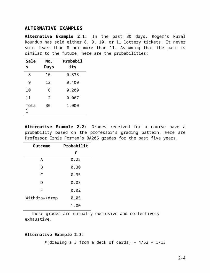
ALTERNATIVE EXAMPLESAlternative Example 2.1:  In the past 30 days, Roger’s Rural Roundup has sold either 8, 9, 10, or 11 lottery tickets. It never sold fewer than 8 nor more than 11. Assuming that the past is similar to the future, here are the probabilities:

Sales No. Days Probability

 8 10 0.333

 9 12 0.400

10 6 0.200

11 2 0.067

Total 30 1.000

Alternative Example 2.2:  Grades received for a course have a probability based on the professor’s grading pattern. Here are Professor Ernie Forman’s BA205 grades for the past five years.

Outcome Probability

A 0.25

B 0.30

C 0.35

D 0.03

F 0.02

Withdraw/drop 0.05

1.00

These grades are mutually exclusive and collectively exhaustive.

Alternative Example 2.3:

P(drawing a 3 from a deck of cards) = 4/52 = 1/13

P(drawing a club on the same draw) = 13/52 = 1/4

These are neither mutually exclusive nor collectively exhaustive.

2-3

Alternative Example 2.4:  In Alternative Example 2.3 we looked at 3s and clubs. Here is the probability for 3 or club:

P(3 or club) = P(3) + P(club) – P(3 and club)

= 4/52 + 13/52 – 1/52

= 16/52 = 4/13

Alternative Example 2.5:  A class contains 30 students. Ten are female (F) and U.S. citizens (U); 12 are male (M) and U.S. citizens; 6 are female and non-U.S. citizens (N); 2 are male and non-U.S. citizens.

A name is randomly selected from the class roster and it is female. What is the probability that the student is a U.S. citizen?

U.S. Not U.S. Total

F 10 6 16

M 12 2 14

Total 22 8 30

P(U | F) = 10/16 = 5/8

Alternative Example 2.6:  Your professor tells you that if you score an 85 or better on your midterm exam, there is a 90% chance you’ll get an A for the course. You think you have only a 50% chance of scoring 85 or better. The probability that both your score is 85 or better and you receive an A in the course is

P(A and 85) = P(A 85) P(85) = (0.90)(0.50) = 0.45

= a 45% chance

2-4

Alternative Example 2.7:  An instructor is teaching two sections (classes) of calculus. Each class has 24 students, and on the surface, both classes appear identical. One class, however, consists of students who have all taken calculus in high school. The instructor has no idea which class is which. She knows that the probability of at least half the class getting As on the first exam is only 25% in an average class, but 50% in a class with more math background.

A section is selected at random and quizzed. More than half the class received As. Now, what is the revised probability that the class was the advanced one?

P(regular class chosen) = 0.5

P(advanced class chosen) = 0.5

P(1/2 As regular class) = 0.25

P(1/2 As advanced class) = 0.50

P(1/2 As and regular class)

= P(1/2 As regular ) P(regular)

= (0.25)(0.50) = 0.125

P(1/2 As and advanced class)

= P(1/2 As advanced) P(advanced)

= (0.50)(0.5) = 0.25

So P(1/2 As) = 0.125 + 0.25 = 0.375

So there is a 66% chance the class tested was the advanced one.

2-5

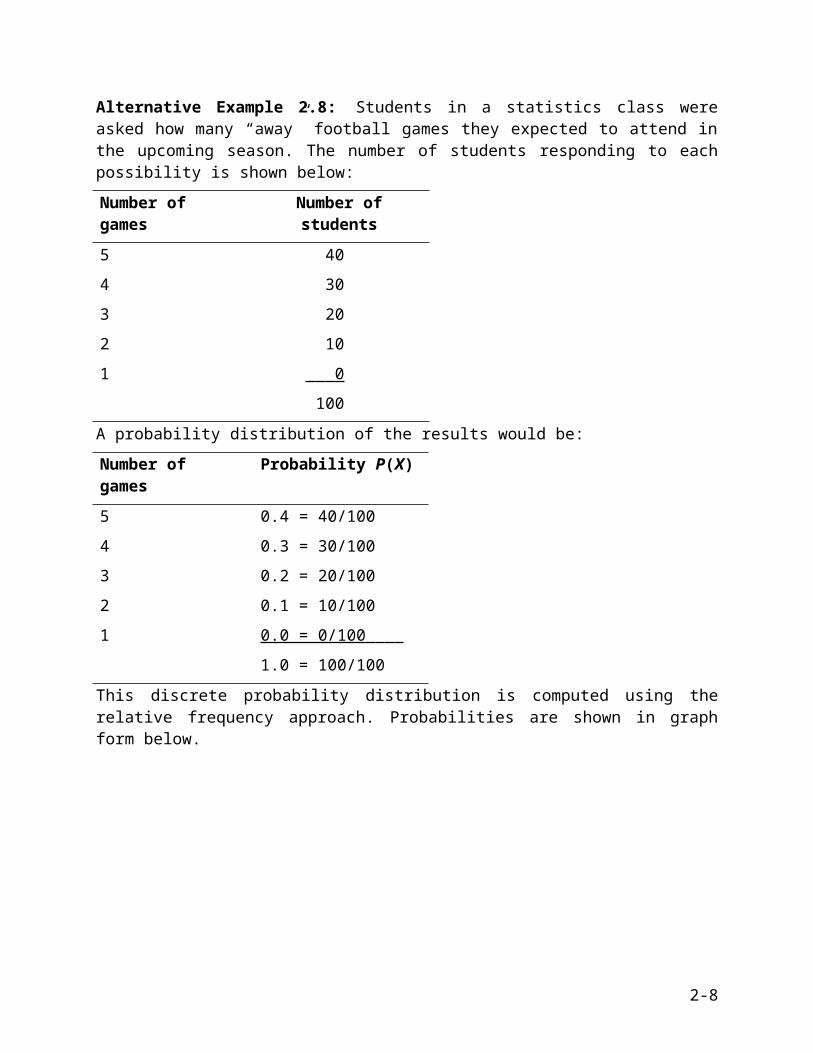
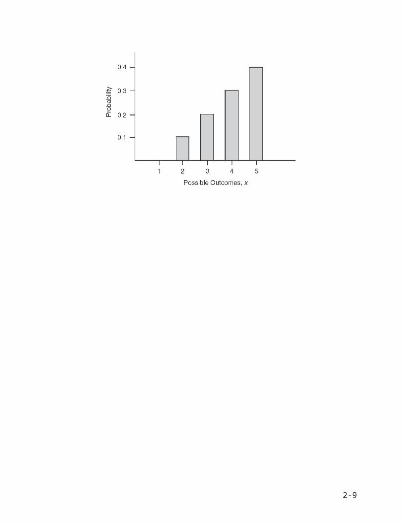
Alternative Example 2.8:  Students in a statistics class were asked how many “away” football games they expected to attend in the upcoming season. The number of students responding to each possibility is shown below:

Number of games Number of students

5 40

4 30

3 20

2 10

1       0

100

A probability distribution of the results would be:

Number of games Probability P(X)

5 0.4 = 40/100

4 0.3 = 30/100

3 0.2 = 20/100

2 0.1 = 10/100

1 0.0 = 0/100        

1.0 = 100/100

This discrete probability distribution is computed using the relative frequency approach. Probabilities are shown in graph form below.

2-6

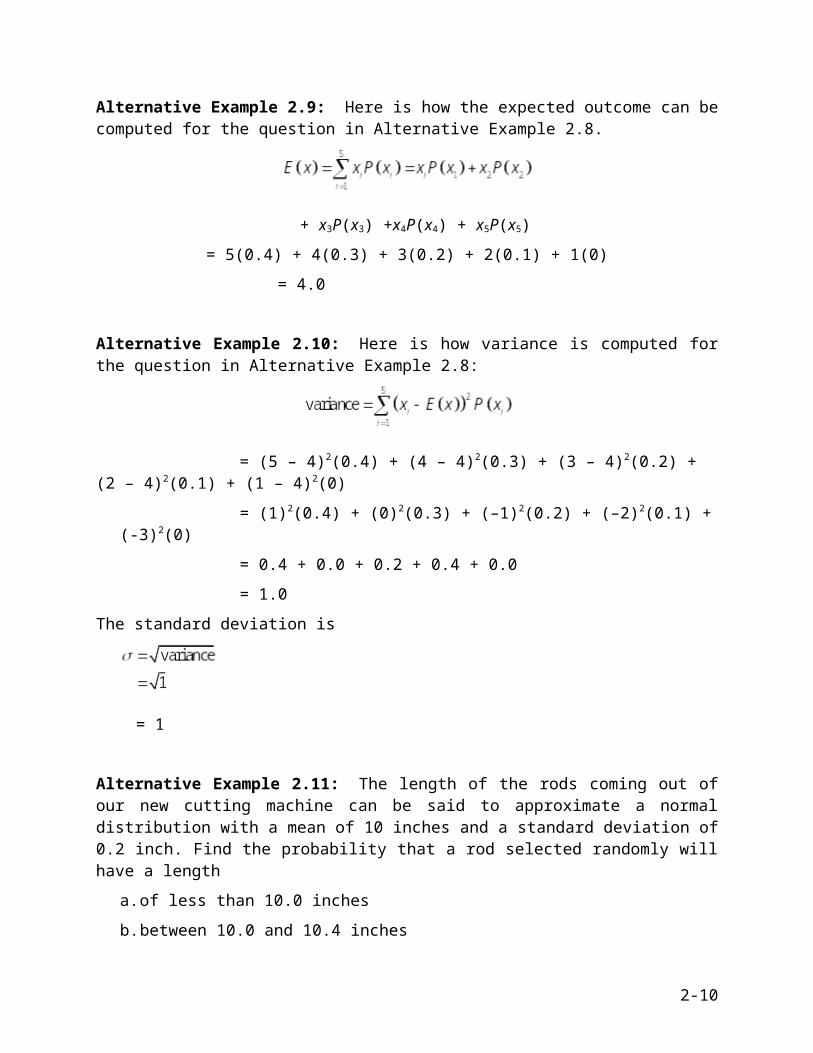
Alternative Example 2.9:  Here is how the expected outcome can be computed for the question in Alternative Example 2.8.

+ x3P(x3) +x4P(x4) + x5P(x5)

= 5(0.4) + 4(0.3) + 3(0.2) + 2(0.1) + 1(0)

= 4.0

Alternative Example 2.10:  Here is how variance is computed for the question in Alternative Example 2.8:

= (5 – 4)2(0.4) + (4 – 4)2(0.3) + (3 – 4)2(0.2) + (2 – 4)2(0.1) + (1 – 4)2(0)

= (1)2(0.4) + (0)2(0.3) + (–1)2(0.2) + (–2)2(0.1) + (-3)2(0)

= 0.4 + 0.0 + 0.2 + 0.4 + 0.0

= 1.0

The standard deviation is

= 1

Alternative Example 2.11:  The length of the rods coming out of our new cutting machine can be said to approximate a normal distribution with a mean of 10 inches and a standard deviation of 0.2 inch. Find the probability that a rod selected randomly will have a length

a. of less than 10.0 inches

b. between 10.0 and 10.4 inches

c. between 10.0 and 10.1 inches

d. between 10.1 and 10.4 inches

e. between 9.9 and 9.6 inches

f. between 9.9 and 10.4 inches

g. between 9.886 and 10.406 inches

2-7

First compute the standard normal distribution, the Z-value:

Next, find the area under the curve for the given Z-value by using a standard normal distribution table.

a. P(x 10.0) = 0.50000

b. P(10.0 x 10.4) = 0.97725 – 0.50000 = 0.47725

c. P(10.0 x 10.1) = 0.69146 – 0.50000 = 0.19146

d. P(10.1 x 10.4) = 0.97725 – 0.69146 = 0.28579

e. P(9.6 x 9.9) = 0.97725 – 0.69146 = 0.28579

f. P(9.9 x 10.4) = 0.19146 + 0.47725 = 0.66871

g. P(9.886 x 10.406) = 0.47882 + 0.21566 = 0.69448

SOLUTIONS TO DISCUSSION QUESTIONS AND PROBLEMS2-1.  There are two basic laws of probability. First, the probability of any event or state of nature occurring must be greater than or equal to zero and less than or equal to 1. Second, the sum of the simple probabilities for all possible outcomes of the activity must equal 1.

2-2.  Events are mutually exclusive if only one of the events can occur on any one trial. Events are collectively exhaustive if the list of outcomes includes every possible outcome. An example of mutually exclusive events can be seen in flipping a coin. The outcome of any one trial can either be a head or a tail. Thus, the events of getting a head and a tail are mutually exclusive because only one of these events can occur on any one trial. This assumes, of course, that the coin does not land on its edge. The outcome of rolling the die is an example of events that are collectively exhaustive. In rolling a standard die, the outcome can be either 1, 2, 3, 4, 5, or 6. These six outcomes are collectively exhaustive because they include all possible outcomes. Again, it is assumed that the die will not land and stay on one of its edges.

2-3.  Probability values can be determined both objectively and subjectively. When determining probability values objectively, some type of numerical or quantitative analysis is used. When determining probability values subjectively, a manager’s or decision maker’s judgment and experience are used in assessing one or more probability values.

2-4.  The probability of the intersection of two events is subtracted in summing the probability of the two events to avoid double counting. For example, if the same event is in both of the probabilities that are to be added, the probability of this event will be included twice unless the intersection of the two events is subtracted from the sum of the probability of the two events.

2-8

2-5.  When events are dependent, the occurrence of one event does have an effect on the probability of the occurrence of the other event. When the events are independent, on the other hand, the occurrence of one of them has no effect on the probability of the occurrence of the other event. It is important to know whether or not events are dependent or independent because the probability relationships are slightly different in each case. In general, the probability relationships for any kind of independent events are simpler than the more generalized probability relationships for dependent events.

2-6.  Bayes’ theorem is a probability relationship that allows new information to be incorporated with prior probability values to obtain updated or posterior probability values. Bayes’ theorem can be used whenever there is an existing set of probability values and new information is obtained that can be used to revise these probability values.

2-7.  A Bernoulli process has two possible outcomes, and the probability of occurrence is constant from one trial to the next. If n independent Bernoulli trials are repeated and the number of outcomes (successes) are recorded, the result is a binomial distribution.

2-8.  A random variable is a function defined over a sample space. There are two types of random variables: discrete and continuous.

2-9.  A probability distribution is a statement of a probability function that assigns all the probabilities associated with a random variable. A discrete probability distribution is a distribution of discrete random variables (that is, random variables with a limited set of values). A continuous probability distribution is concerned with a random variable having an infinite set of values. The distributions for the number of sales for a salesperson is an example of a discrete probability distribution, whereas the price of a product and the ounces in a food container are examples of a continuous probability distribution.

2-10.  The expected value is the average of the distribution and is computed by using the following formula: E(X) = X · P(X) for a discrete probability distribution.

2-11.  The variance is a measure of the dispersion of the distribution. The variance of a discrete probability distribution is computed by the formula

2 = [X – E(X)]2P(X)

2-12.  The purpose of this question is to have students name three business processes they know that can be described by a normal distribution. Answers could include sales of a product, project completion time, average weight of a product, and product demand during lead or order time.

2-13.  This is an example of a discrete probability distribution. It was most likely computed using historical data. It is important to note that it follows the laws of a probability distribution. The total sums to 1, and the individual values are less than or equal to 1.

2-9

2-14.

Grade Probability

A

B

C

D

F

1.0

Thus, the probability of a student receiving a C in the course is 0.30 = 30%.

The probability of a student receiving a C may also be calculated using the following equation:

= 0.30

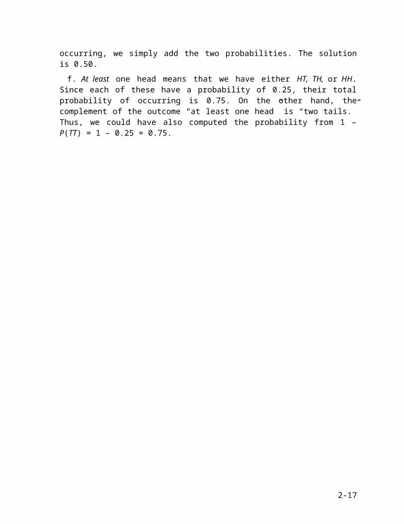
2-15. a. P(H) = 1/2 = 0.5

b. P(T H) = P(T) = 0.5

c. P(TT) = P(T) P(T) = (0.5)(0.5) = 0.25

d. P(TH) = P(T) P(H) = (0.5)(0.5) = 0.25

e. We first calculate P(TH) = 0.25, then calculate P(HT) = (0.5)(0.5) = 0.25. To find the probability of either one occurring, we simply add the two probabilities. The solution is 0.50.

f. At least one head means that we have either HT, TH, or HH. Since each of these have a probability of 0.25, their total probability of occurring is 0.75. On the other hand, the complement of the outcome “at least one head” is “two tails.” Thus, we could have also computed the probability from 1 – P(TT) = 1 – 0.25 = 0.75.

2-10

2-16. The distribution of chips is as follows:

Red   8

Green 10

White     2

 Total = 20

a. The probability of drawing a white chip on the first draw is

b. The probability of drawing a white chip on the first draw and a red one on the second is

P(WR) = P(W) P(R)

(the two events are independent)

= (0.10)(0.40)

= 0.04

c. P(GG) = P(G) P(G)

= (0.5)(0.5)

= 0.25

d. P(R W) = P(R) (the events are independent and hence the conditional probability equals the marginal probability)

= 0.40

2-11

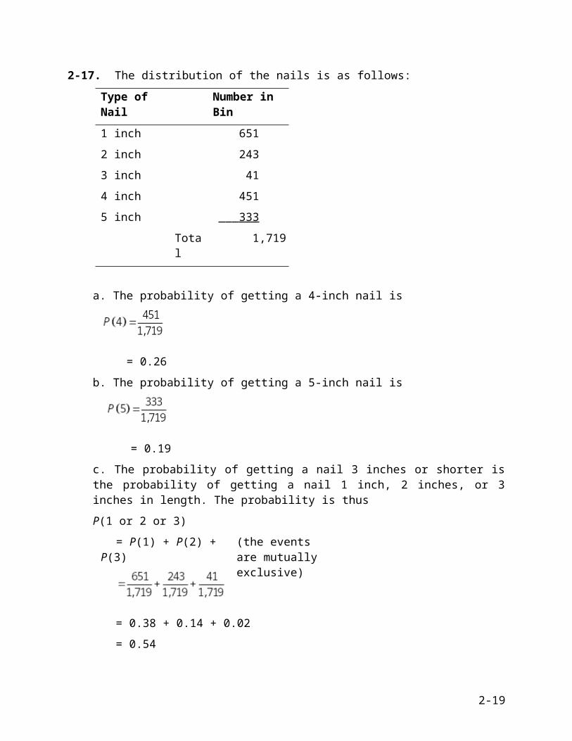
2-17.  The distribution of the nails is as follows:

Type of Nail Number in Bin

1 inch 651

2 inch 243

3 inch 41

4 inch 451

5 inch       333

Total 1,719

a. The probability of getting a 4-inch nail is

= 0.26

b. The probability of getting a 5-inch nail is

= 0.19

c. The probability of getting a nail 3 inches or shorter is the probability of getting a nail 1 inch, 2 inches, or 3 inches in length. The probability is thus

P(1 or 2 or 3)

= P(1) + P(2) + P(3) (the events are mutually exclusive)

= 0.38 + 0.14 + 0.02

= 0.54

2-12

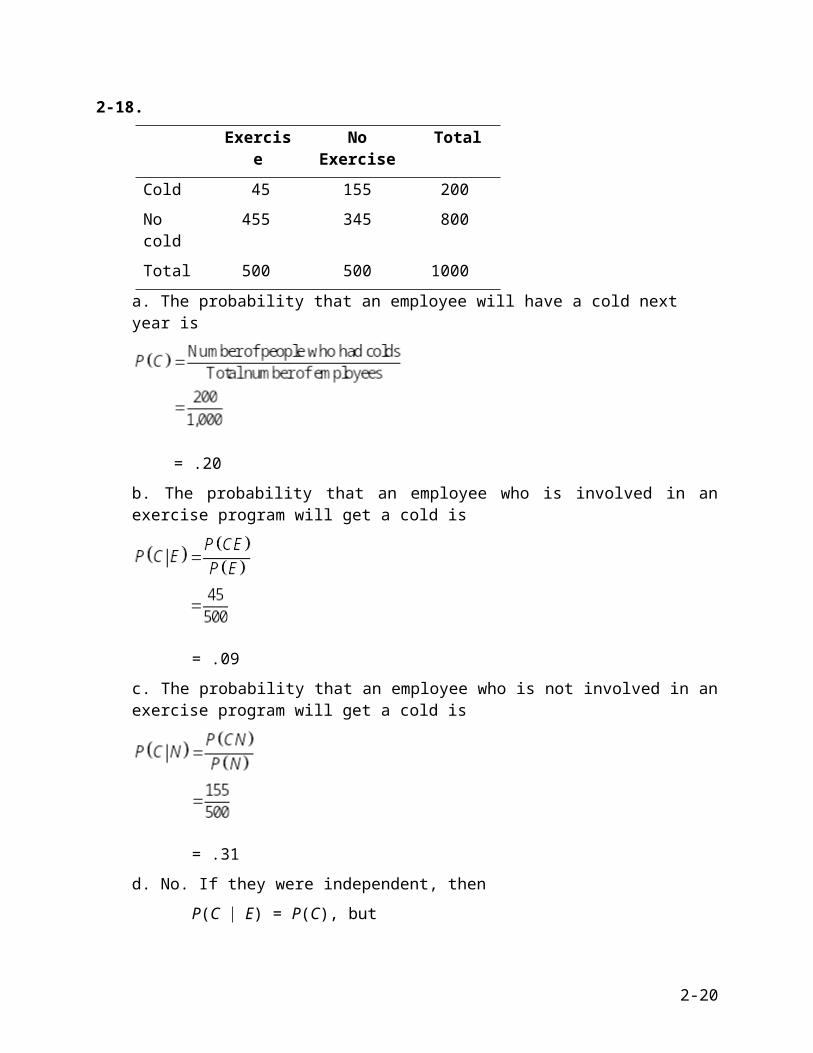
2-18.

Exercise No Exercise Total

Cold 45 155 200

No cold 455 345 800

Total 500 500 1000

a. The probability that an employee will have a cold next year is

= .20

b. The probability that an employee who is involved in an exercise program will get a cold is

= .09

c. The probability that an employee who is not involved in an exercise program will get a cold is

= .31

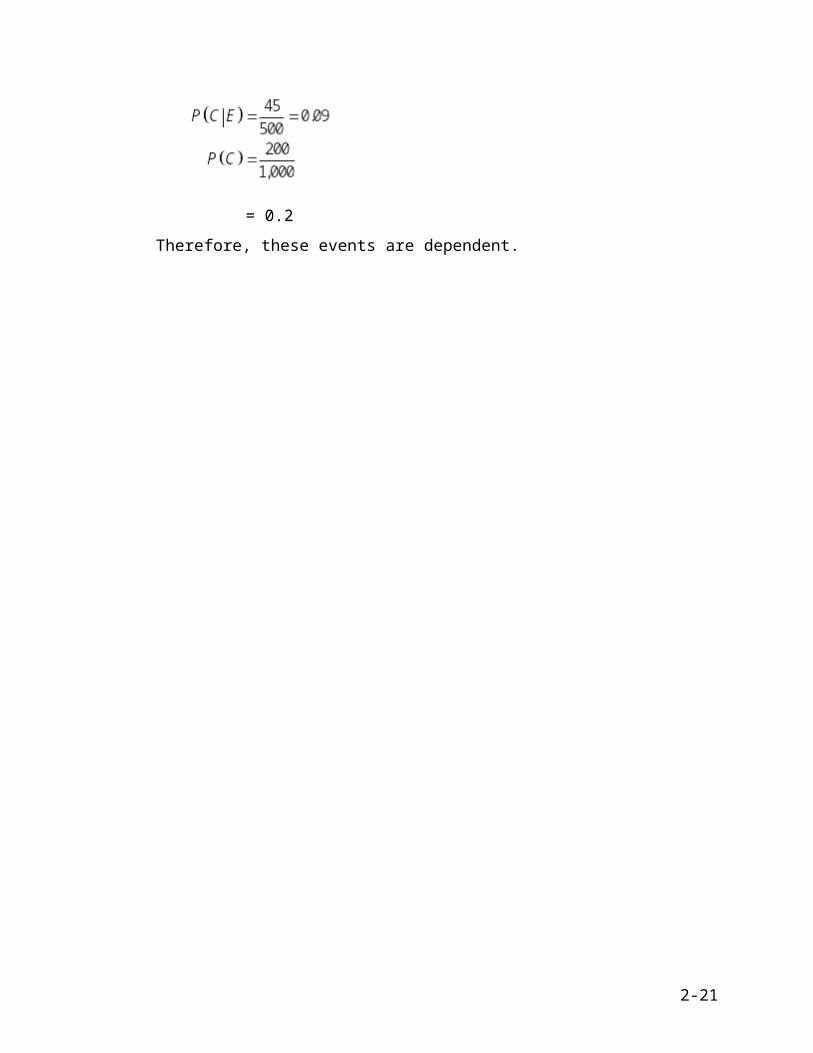
d. No. If they were independent, then

P(C E) = P(C), but

= 0.2

2-13

Therefore, these events are dependent.

2-14

2-19.  The probability of winning tonight’s game is

= 0.6

The probability that the team wins tonight is 0.60. The probability that the team wins tonight and draws a large crowd at tomorrow’s game is a joint probability of dependent events. Let the probability of winning be P(W) and the probability of drawing a large crowd be P(L). Thus

P(WL) = P(L W) P(W) (the probability of large crowd is 0.90 if the team wins tonight)

= 0.90 0.60

= 0.54

Thus, the probability of the team winning tonight and of there being a large crowd at tomorrow’s game is 0.54.

2-20.  The second draw is not independent of the first because the probabilities of each outcome depend on the rank (sophomore or junior) of the first student’s name drawn. Let

J1 = junior on first draw

J2 = junior on second draw

S1 = sophomore on first draw

S2 = sophomore on second draw

a. P(J1) = 3/10 = 0.3

b. P(J2 S1) = 0.3

c. P(J2 J1) = 0.8

d. P(S1S2) = P(S2 S1) P(S1) = (0.7)(0.7)

= 0.49

e. P(J1J2) = P(J2 J1) P(J1) = (0.8)(0.3) = 0.24

f. P(1 sophomore and 1 junior regardless of order) is P(S1J2) + P(J1S2)

P(S1J2) = P(J2 S1) P(S1) = (0.3)(0.7) = 0.21

P(J1S2) = P(S2 J1) P(J1) = (0.2)(0.3) = 0.06

Hence, P(S1J2) + P(J1S2) = 0.21 + 0.06 = 0.27.

2-15

2-21.  Without any additional information, we assume that there is an equally likely probability that the soldier wandered into either oasis, so P(Abu Ilan) = 0.50 and P(El Kamin) = 0.50. Since the oasis of Abu Ilan has 20 Bedouins and 20 Farimas (a total population of 40 tribesmen), the probability of finding a Bedouin, given that you are in Abu Ilan, is 20/40 = 0.50. Similarly, the probability of finding a Bedouin, given that you are in El Kamin, is 32/40 = 0.80. Thus, P(Bedouin Abu Ilan) = 0.50, P(Bedouin El Kamin) = 0.80.

We now calculate joint probabilities:

P(Abu Ilan and Bedouin) = P(Bedouin Abu Ilan) P(Abu Ilan)

= (0.50)(0.50) = 0.25

P(El Kamin and Bedouin)

= P(Bedouin El Kamin)  P(El Kamin) = (0.80)(0.50)

= 0.4

The total probability of finding a Bedouin is

P(Bedouin) = 0.25 + 0.40 = 0.65

P(Abu Ilan Bedouin)

P(El Kamin Bedouin)

The probability the oasis discovered was Abu Ilan is now only 0.385. The probability the oasis is El Kamin is 0.615.

2-16

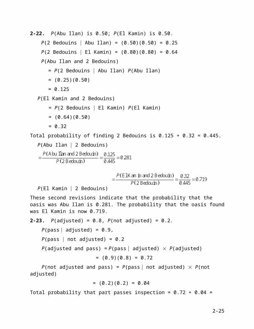
2-22.  P(Abu Ilan) is 0.50; P(El Kamin) is 0.50.

P(2 Bedouins Abu Ilan) = (0.50)(0.50) = 0.25

P(2 Bedouins El Kamin) = (0.80)(0.80) = 0.64

P(Abu Ilan and 2 Bedouins)

= P(2 Bedouins Abu Ilan) P(Abu Ilan)

= (0.25)(0.50)

= 0.125

P(El Kamin and 2 Bedouins)

= P(2 Bedouins El Kamin) P(El Kamin)

= (0.64)(0.50)

= 0.32

Total probability of finding 2 Bedouins is 0.125 + 0.32 = 0.445.

P(Abu Ilan 2 Bedouins)

P(El Kamin 2 Bedouins)

These second revisions indicate that the probability that the oasis was Abu Ilan is 0.281. The probability that the oasis found was El Kamin is now 0.719.

2-23.  P(adjusted) = 0.8, P(not adjusted) = 0.2.

P(pass adjusted) = 0.9,

P(pass not adjusted) = 0.2

P(adjusted and pass) = P(pass adjusted) P(adjusted)

= (0.9)(0.8) = 0.72

P(not adjusted and pass) = P(pass not adjusted) P(not adjusted)

= (0.2)(0.2) = 0.04

Total probability that part passes inspection = 0.72 + 0.04 = 0.76

P(adjusted pass)

The posterior probability the lathe tool is properly adjusted is 0.947.

2-17

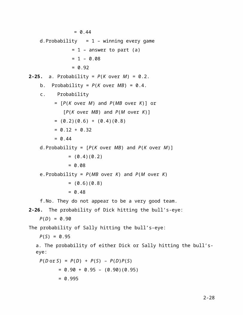
2-24. MB = Mama’s Boys, K = the Killers, and M = the Machos

a. The probability that K will win every game is

P = P(K over MB) and P(K over M)

= (0.4)(0.2 ) = 0.08

b. The probability that M will win at least one game is

P(M over K) + P(M over MB) – P(M over K) P(M over MB)

= (0.8) + (0.2) – (0.8)(0.2)

= 1 – 0.16

= 0.84

c. The probability is

1. [P(MB over K) and P(M over MB)], or

2. [P(MB over M) and P(K over MB)]

P(1) = (0.6)(0.2) = 0.12

P(2) = (0.8)(0.4) = 0.32

Probability = P(1) + P(2)

= 0.12 + 0.32

= 0.44

d. Probability = 1 – winning every game

2-18

= 1 – answer to part (a)

= 1 – 0.08

= 0.92

2-25.  a. Probability = P(K over M) = 0.2.

b. Probability = P(K over MB) = 0.4.

c. Probability

= [P(K over M) and P(MB over K)] or

   [P(K over MB) and P(M over K)]

= (0.2)(0.6) + (0.4)(0.8)

= 0.12 + 0.32

= 0.44

d. Probability = [P(K over MB) and P(K over M)]

  = (0.4)(0.2)

  = 0.08

e. Probability = P(MB over K) and P(M over K)

  = (0.6)(0.8)

  = 0.48

f. No. They do not appear to be a very good team.

2-26.  The probability of Dick hitting the bull’s-eye:

   P(D) = 0.90

The probability of Sally hitting the bull’s-eye:

   P(S) = 0.95

a. The probability of either Dick or Sally hitting the bull’s-eye:

   P(D or S) = P(D) + P(S) – P(D)P(S)

= 0.90 + 0.95 – (0.90)(0.95)

= 0.995

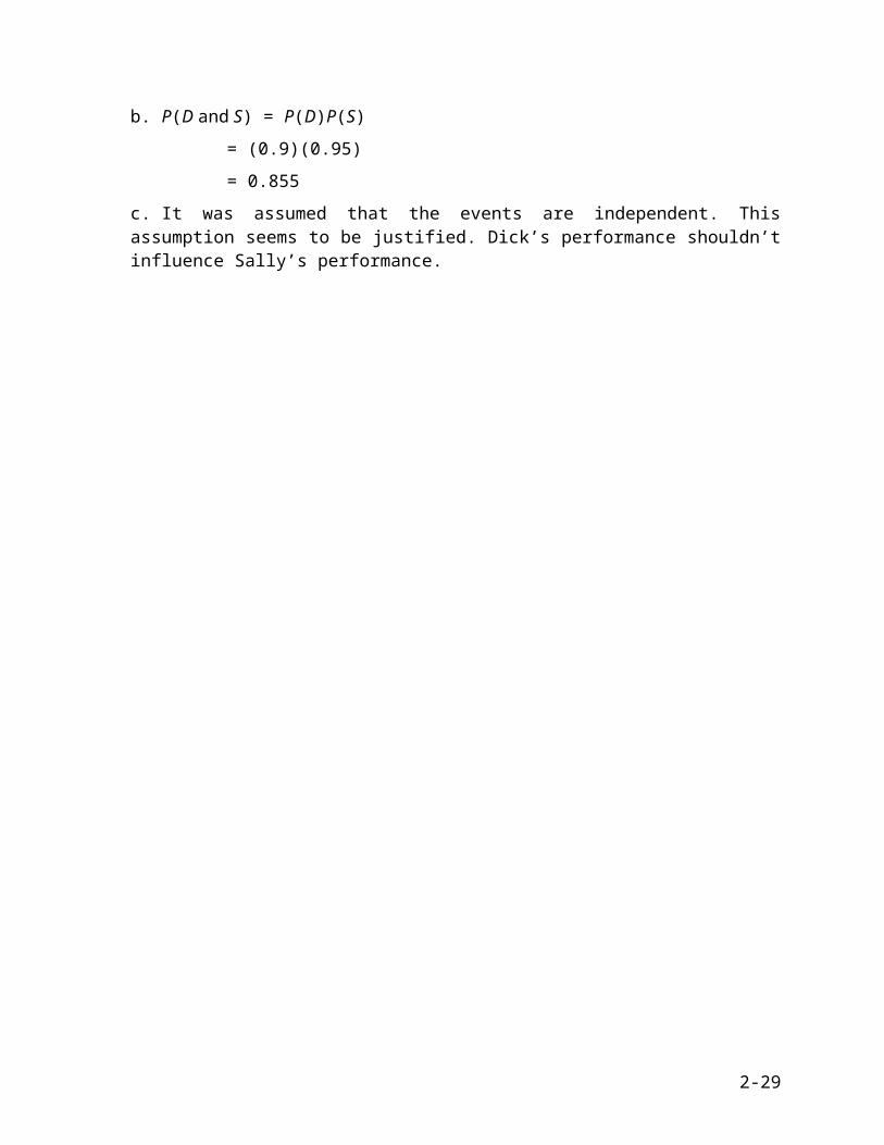
b. P(D and S) = P(D)P(S)

= (0.9)(0.95)

= 0.855

c. It was assumed that the events are independent. This assumption seems to be justified. Dick’s performance shouldn’t influence Sally’s performance.

2-19

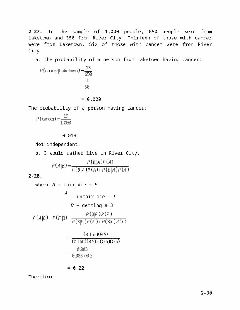
2-27.  In the sample of 1,000 people, 650 people were from Laketown and 350 from River City. Thirteen of those with cancer were from Laketown. Six of those with cancer were from River City.

a. The probability of a person from Laketown having cancer:

= 0.020

The probability of a person having cancer:

= 0.019

Not independent.

b. I would rather live in River City.

2-28.   

where A = fair die = F

           = unfair die = L

          B = getting a 3

= 0.22

Therefore,

P(L) = 1 – 0.22 = 0.78

2-29.  Parts (a) and (c) are probability distributions because the probability values for each event are between 0 and 1, and the sum of the probability values for the events is 1.

2-20

2-21

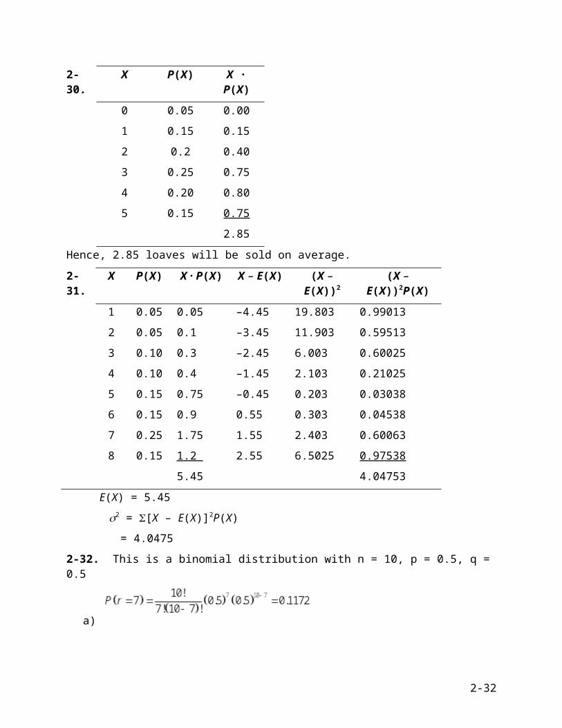
2-30. X P(X) X · P(X)

0 0.05 0.00

1 0.15 0.15

2 0.2 0.40

3 0.25 0.75

4 0.20 0.80

5 0.15 0.75

2.85

Hence, 2.85 loaves will be sold on average.

2-31. X P(X) X · P(X) X – E(X) (X – E(X))2 (X – E(X))2P(X)

1 0.05 0.05 –4.45 19.803 0.99013

2 0.05 0.1 –3.45 11.903 0.59513

3 0.10 0.3 –2.45 6.003 0.60025

4 0.10 0.4 –1.45 2.103 0.21025

5 0.15 0.75 –0.45 0.203 0.03038

6 0.15 0.9 0.55 0.303 0.04538

7 0.25 1.75 1.55 2.403 0.60063

8 0.15 1 .2   2.55 6.5025 0 .97538

5.45 4.04753

E(X) = 5.45

2 = [X – E(X)]2P(X)

= 4.0475

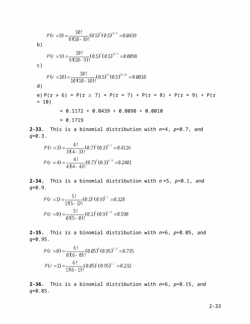
2-32.  This is a binomial distribution with n = 10, p = 0.5, q = 0.5

a) 

b) 

c) 

2-22

d) 

e) P(r 6) = P(r 7) = P(r = 7) + P(r = 8) + P(r = 9) + P(r = 10)

= 0.1172 + 0.0439 + 0.0098 + 0.0010

= 0.1719

2-33.  This is a binomial distribution with n=4, p=0.7, and q=0.3.

  

2-34.  This is a binomial distribution with n =5, p=0.1, and q=0.9.

  

2-35.  This is a binomial distribution with n=6, p=0.05, and q=0.95.

  

2-36.  This is a binomial distribution with n=6, p=0.15, and q=0.85.

 

Probability of 0 or 1 defective = P(0) + P(1) = 0.377 + 0.399 = 0.776.

2-23

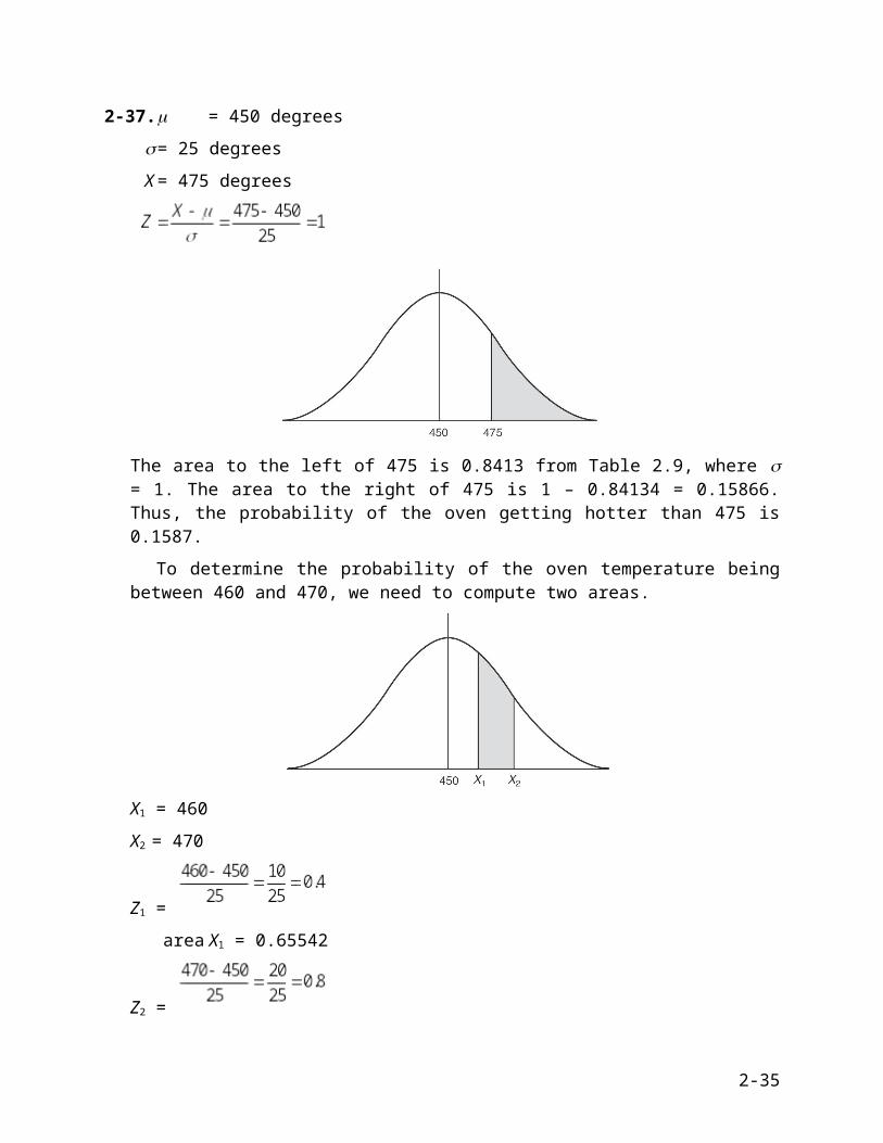
2-37. = 450 degrees

= 25 degrees

X= 475 degrees

The area to the left of 475 is 0.8413 from Table 2.9, where = 1. The area to the right of 475 is 1 – 0.84134 = 0.15866. Thus, the probability of the oven getting hotter than 475 is 0.1587.

To determine the probability of the oven temperature being between 460 and 470, we need to compute two areas.

X1 = 460

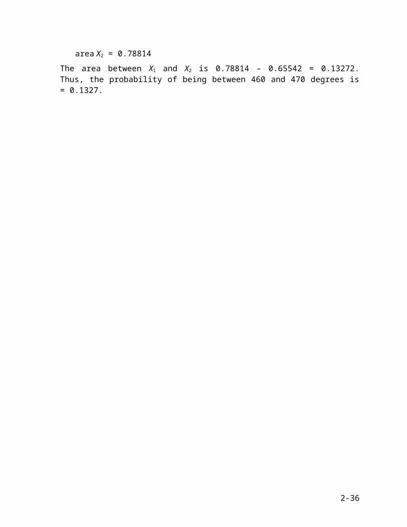
X2 = 470

Z1 =

area X1 = 0.65542

Z2 =

area X2 = 0.78814

The area between X1 and X2 is 0.78814 – 0.65542 = 0.13272. Thus, the probability of being between 460 and 470 degrees is = 0.1327.

2-24

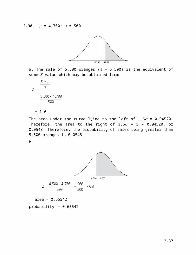
2-38.   = 4,700; = 500

a. The sale of 5,500 oranges (X = 5,500) is the equivalent of some Z value which may be obtained from

Z =

=

= 1.6

The area under the curve lying to the left of 1.6 = 0.94520. Therefore, the area to the right of 1.6 = 1 – 0.94520, or 0.0548. Therefore, the probability of sales being greater than 5,500 oranges is 0.0548.

b.

area = 0.65542

probability= 0.65542

2-25

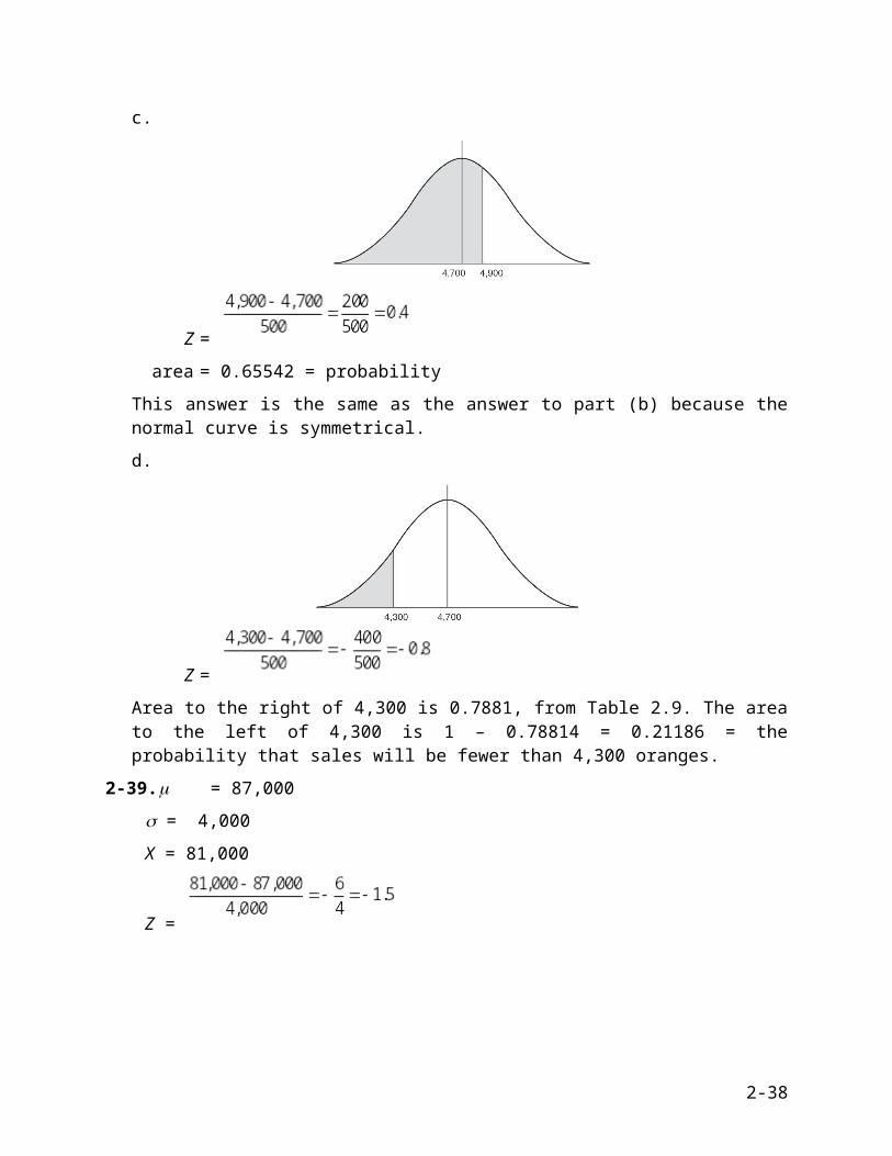
c.

Z =

area = 0.65542 = probability

This answer is the same as the answer to part (b) because the normal curve is symmetrical.

d.

Z =

Area to the right of 4,300 is 0.7881, from Table 2.9. The area to the left of 4,300 is 1 – 0.78814 = 0.21186 = the probability that sales will be fewer than 4,300 oranges.

2-39. = 87,000

=  4,000

X = 81,000

Z =

2-26

Area to the right of 81,000 = 0.93319, from Table 2.9, where Z = 1.5. Thus, the area to the left of 81,000 = 1 – 0.93319 = 0.06681 = the probability that sales will be fewer than 81,000 packages.

2-40.

= 457,000

Ninety percent of the time, sales have been between 460,000 and 454,000 pencils. This means that 10% of the time sales have exceeded 460,000 or fallen below 454,000. Since the curve is symmetrical, we assume that 5% of the area lies to the right of 460,000 and 5% lies to the left of 454,000. Thus, 95% of the area under the curve lies to the left of 460,000. From Table 2.9, we note that the number nearest 0.9500 is 0.94950. This corresponds to a Z value of 1.64. Therefore, we may conclude that the Z value corresponding to a sale of 460,000 pencils is 1.64.

Using Equation 2-15, we get

X = 460,000

= 457,000

is unknown

Z = 1.64

1.64 = 3000

= 1829.27

2-41.  The time to complete the project (X) is normally distributed with = 60 and = 4.

a) P(X 62) = P(Z (62 – 60)/4) = P(Z 0.5) = 0.69146

    b) P(X 66) = P(Z (66 – 60)/4) = P(Z 1.5) = 0.93319

   c) P(X 65) = 1 – P(X 65)

 = 1 – P(Z (65 – 60)/4)

2-27

 = 1 – P(Z 1.25)

 = 1 – 0.89435 = 0.10565

2-28

2-42.  The time to complete the project (X) is normally distributed with = 40 and = 5. A penalty must be paid if the project takes longer than the due date (or if X due date).

a) P(X 40) = 1 – (X 40) = 1 – P(Z (40 – 40)/5) = 1 – P(Z 0) = 1 – 0.5 = 0.5

b) P(X 43) = 1 – P(X 43) = 1 – P(Z (43 – 40)/5) = 1 – P(Z 0.6) = 1 – 0.72575 = 0.27425

c) If there is a 5% chance that the project will be late, there is a 95% chance the project will be finished by the due date. So,

P(X due date) = 0.95 or

P(X _____) = 0.95

The Z-value for a probability of 0.95 is approximately 1.64, so the due date (X) should have a Z-value of 1.64. Thus,

5(1.64) = X – 40

X = 48.2.

The due date should be 48.2 weeks from the start of the project

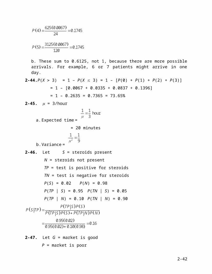
2-43.   = 5/day; e– = 0.0067 (from Appendix C)

a.

b. These sum to 0.6125, not 1, because there are more possible arrivals. For example, 6 or 7 patients might arrive in one day.

2-29

2-44. P(X 3) = 1 – P(X 3) = 1 – [P(0) + P(1) + P(2) + P(3)]

= 1 – [0.0067 + 0.0335 + 0.0837 + 0.1396]

= 1 – 0.2635 = 0.7365 = 73.65%

2-45.   = 3/hour

a. Expected time =

= 20 minutes

b. Variance =

2-46.  Let S = steroids present

N = steroids not present

TP = test is positive for steroids

TN = test is negative for steroids

P(S) = 0.02 P(N) = 0.98

P(TP | S) = 0.95 P(TN | S) = 0.05

P(TP | N) = 0.10 P(TN | N) = 0.90

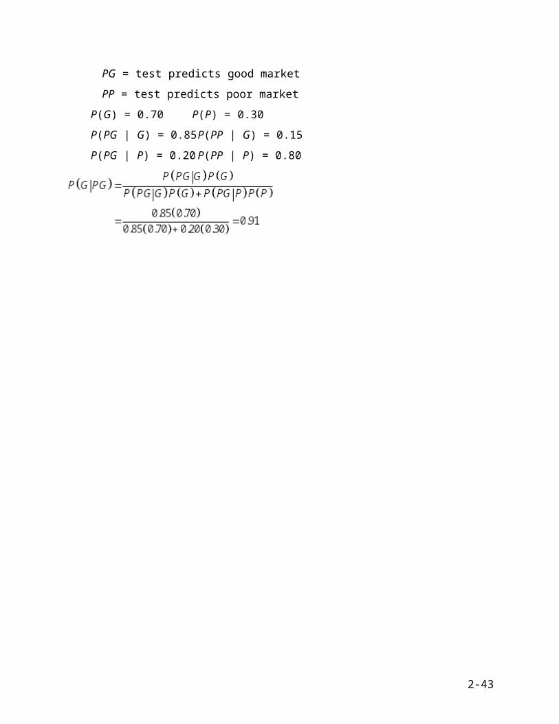
2-47.  Let G = market is good

       P = market is poor

    PG = test predicts good market

    PP = test predicts poor market

P(G) = 0.70 P(P) = 0.30

P(PG | G) = 0.85 P(PP | G) = 0.15

P(PG | P) = 0.20 P(PP | P) = 0.80

2-30

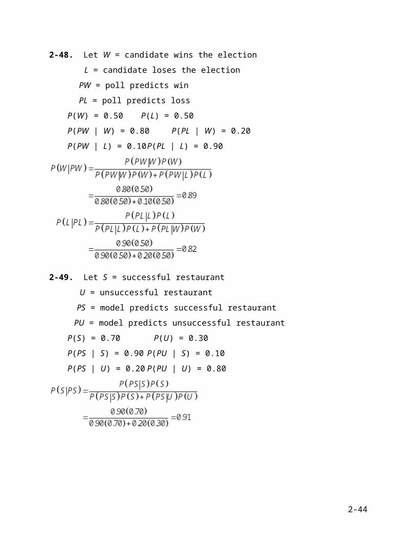
2-48.  Let W = candidate wins the election

        L = candidate loses the election

 PW = poll predicts win

 PL = poll predicts loss

P(W) = 0.50 P(L) = 0.50

P(PW | W) = 0.80 P(PL | W) = 0.20

P(PW | L) = 0.10 P(PL | L) = 0.90

2-49.  Let S = successful restaurant

U = unsuccessful restaurant

PS = model predicts successful restaurant

PU = model predicts unsuccessful restaurant

P(S) = 0.70 P(U) = 0.30

P(PS | S) = 0.90 P(PU | S) = 0.10

P(PS | U) = 0.20 P(PU | U) = 0.80

2-31

2-50.  Let D = Default on loan; D' = No default; R = Loan rejected; R = Loan approved Given:

P(D) = 0.2

P(D') = 0.8

P(R | D) = 0.9

P(R' | D') = 0.7

(a) P(R | D') = 1 – 0.7 = 0.3

(b)

2-51. (a) F0.05, 5, 10 = 3.33

(b) F0.05, 8.7 = 3.73

(c) F0.05, 3, 5 = 5.41

(d) F0.05, 10. 4 = 5.96

2-52. (a) F0.01, 15, 6 = 7.56

(b) F0.01, 12, 8 = 5.67

(c) F0.01, 3, 5 = 12.06

(d) F0.01, 9, 7 = 6.72

2-53. (a) From the appendix, P(F3,4 6.59) = 0.05, so P(F 6.8) must be less than 0.05.

(b) From the appendix, P(F7,3 8.89) = 0.05, so P(F 3.6) must be greater than 0.05.

(c) From the appendix, P(F20,20 2.12) = 0.05, so P(F 2.6) must be less than 0.05.

(d) From the appendix, P(F7,5 4.88) = 0.05, so P(F 5.1) must be less than 0.05.

(e) From the appendix, P(F7,5 4.88) = 0.05, so P(F 5.1) must be greater than 0.05.

2-32

2-54. (a) From the appendix, P(F5,4 15.52) = 0.01, so P(F 14) must be greater than 0.01.

(b) From the appendix, P(F6,3 27.91) = 0.01, so P(F 30) must be less than 0.01.

(c) From the appendix, P(F10,12 4.30) = 0.01, so P(F 4.2) must be greater than 0.01.

(d) From the appendix, P(F2,3 30.82) = 0.01, so P(F 35) must be less than 0.01.

(e) From the appendix, P(F2,3 30.82) = 0.01, so P(F 35) must be greater than 0.01.

2-55. Average time = 4 minutes = 1/µ. So µ = ¼ = 0.25

(a) P(X < 3) = 1 – e-0.25(3) = 1 – 0.4724 = 0.5276

(b) P(X < 4) = 1 – e-0.25(4) = 1 – 0.3679 = 0.6321

(c) P(X < 5) = 1 – e-0.25(5) = 1 – 0.2865 = 0.7135

(d) P(X > 5) = e-0.25(5) = 0.2865

2-56. Average number per minute = 5. So λ = 5

(a) P(X is exactly 5) = P(5) = (55e-5)/5! = 0.1755

(b) P(X is exactly 4) = P(4) = (54e-5)/4! = 0.1755

(c) P(X is exactly 3) = P(3) = (53e-5)/3! = 0.1404

(d) P(X is exactly 6) = P(6) = (56e-5)/6! = 0.1462

(e) P(X< 2) = P(X is 0 or 1) = P(0) + P(1) = 0.0067 + 0.0337 = 0.0404

2-57. The average time to service a customer is 1/3 hour or 20 minutes. The average number that would be served per minute (µ) is 1/20 = 0.05 per minute.

P(time < ½ hour) = P(time < 30 minutes) = P(X < 30) = 1 – e-0.05(30) = 0.7769

P(time < 1/3 hour) = P(time < 20 minutes) = P(X < 20) = 1 – e-0.05(20) = 0.6321

P(time < 2/3 hour) = P(time < 40 minutes) = P(X < 40) = 1 – e-0.05(40) = 0.8647

These are exactly the same probabilities shown in the example.

2-33

2-58. X = 280

= 250

= 25

= 1.20 standard deviations

From Table 2.9, the area under the curve corresponding to a Z of 1.20 = 0.88493. Therefore, the probability that the sales will be less than 280 boats is 0.8849.

2-34

2-59. The probability of sales being over 265 boats:

X = 265

= 250

= 25

= 0.60

From Table 2.9, we find that the area under the curve to the left of Z = 0.60 is 0.72575. Since we want to find the probability of selling more than 265 boats, we need the area to the right of Z = 0.60. This area is 1 – 0.72575, or 0.27425. Therefore, the probability of selling more than 265 boats = 0.2743.

For a sale of fewer than 250 boats:

X = 250

= 250

= 25

However, a sale of 250 boats corresponds to = 250. At this point, Z = 0. The area under the curve that concerns us is that half of the area lying to the left of = 250. This area = 0.5000. Thus, the probability of selling fewer than 250 boats = 0.5.

2-35

2-60. = 0.55 inch (average shaft size)

X = 0.65 inch

= 0.10 inch

Converting to a Z value yields

= 1

We thus need to look up the area under the curve that lies to the left of 1. From Table 2.9, this is seen to be = 0.84134. As seen earlier, the area to the left of is = 0.5000.

We are concerned with the area between and + 1. This is given by the difference between 0.84134 and 0.5000, and it is 0.34134. Thus, the probability of a shaft size between 0.55 inch and 0.65 inch = 0.3413.

2-61. Greater than 0.65 inch:

area to the left of 1 = 0.84134

area to the right of 1 = 1 – 0.84134

= 0.15866

Thus, the probability of a shaft size being greater than 0.65 inch is 0.1587.

2-36

The shaft size between 0.53 and 0.59 inch:

X2 = 0.53 inch

X1 = 0.59 inch

= 0.55 inch

Converting to scores:

Since Table 2.9 handles only positive Z values, we need to calculate the probability of the shaft size being greater than 0.55 + 0.02 = 0.57 inch. This is determined by finding the area to the left of 0.57, that is, to the left of 0.2. From Table 2.9, this is 0.57926. The area to the right of 0.2 is 1 – 0.57926 = 0.42074. The area to the left of 0.53 is also 0.42074 (the curve is symmetrical). The area to the left of 0.4 is 0.65542. The area between X1 and X2 is 0.65542 – 0.42074 = 0.23468. The probability that the shaft will be between 0.53 inch and 0.59 inch is 0.2347.

Under 0.45 inch:

X = 0.45

= 0.55

= 0.10

2-37

= –1

Thus, we need to find the area to the left of –1. Again, since Table 2.9 handles only positive values of Z, we need to determine the area to the right of 1. This is obtained by 1 – 0.84134 = 0.15866 (0.84134 is the area to the left of 1). Therefore, the area to the left of –1 = 0.15866 (the curve is symmetrical). Thus, the probability that the shaft size will be under 0.45 inch is 0.1587.

2-62.

x = 3

n = 4

q = 15/20 = .75

p = 5/20 = .25

(4)(.0156)(.75) =

.0468   [probability that Marie will win 3 games]

   [probability that Marie will win all four games against Jan]

2-38

Probability that Marie will be number one is .04698 + .003906 = .050886.

2-39

2-63. Probability one will be fined =P(2) + P(3) + P(4) + P(5)= 1 – P(0) – P(1)

= 1 – .03125 – .15625= .08125

Probability of no foul outs = P(0) = 0.03125Probability of foul out in all 5 games = P(5) = 0.03125

2-64.

X P(X)

0 .327

1 .410

2 .205

3 .051

4 .0064

5 .00032

1.0

XP(X) X – E(X) (X – E(X))2 (X – E(X))2P(X)

0.0 –.9985 .997  .326.41 .0015 0 0.41 1.0015 1.003 .2056.153 2.0015 4.006 .2043.024 3.0015 9.009 .0541.0015 4.0015 16.012 .0048 .9985 .7948

E(X) = .9985 1.0     2 = (X – E(X))2P(X)

2-40

= .7948 0.80

2-41

Using the formulas for the binomial:E(X) = np

= (5)(.2) = 1.02 = np(1 – p)

= 5(.2)(.8)= 0.80

The equation produced equivalent results.

2-65. a. n = 10; p = .25; q = .75;

P(X) X

.0563 0

.1877 1

.2816 2

.2503 3

.1460 4

.0584 5

.0162 6

.0031 7

.0004 8

2-42

.00003 9

.0000 10

b.  E(X) = (10).25 = 2.5

2 = npq = (10)(.25)(.75)

= 1.875

c.  Expected weekly profit:

$125.

      2.5

$312.50

SOLUTION TO WTVX CASE1.  The chances of getting 15 days of rain during the next 30 days can be computed by using the binomial theorem. The problem is well suited for solution by the theorem because there are two and only two possible outcomes (rain or shine) with given probabilities (70% and 30%, respectively). The formula used is:

Probability of r successes =

where

n = the number of trials (in this case, the number of days = 30),

r = the number of successes (number of rainy days = 15),

p = probability of success (probability of rain = 70%), and

q = probability of failure (probability of shine = 30%).

The probability of getting exactly 15 days of rain in the next 30 days is 0.0106 or a 1.06% chance.

2.  Joe’s assumptions concerning the weather for the next 30 days state that what happens on one day is not in any way dependent on what happened the day before; what this says, for example, is that if a cold front passed through yesterday, it will not affect what happens today.

But there are perhaps certain conditional probabilities associated with the weather (for example, given that it rained yesterday, the probability of rain today is 80% as opposed to 70%).

2-43

Not being familiar with the field of meteorology, we cannot say precisely what these are. However, our contention is that these probabilities do exist and that Joe’s assumptions are fallacious.

2-44