UNIVERSAL LIQUID MIXTURE MODELS FOR VAPOR-LIQUID AND LIQUID- LIQUID EQUILIBRIA IN HEXANE-BUTANOL

-WATER SYSTEM

by

Akand Wahid Islam

A thesis submitted to the graduate faculty in partial fulfillment of the requirements for the degree of

MASTER OF SCIENCE

Department: Chemical Engineering Major: Chemical Engineering

Major Professor: Dr. Vinayak Kabadi

North Carolina A&T State University Greensboro, North Carolina

2009

 

iii

BIOGRAPHICAL SKETCH

Akand Wahid Islam was born on 26 October, 1980 in Madaripur, Bangladesh. He

received his Bachelor of Science degree in Chemical Engineering from Bangladesh

University of Engineering and Technology (BUET), Bangladesh, in 2005. He is a

candidate for the Master of Science degree in Chemical Engineering.

 

iv

ACKNOWLEDGMENTS

I wish to express my sincerest gratitude to the individuals who supported and

encouraged me both professionally and personally in the completion of this work.

Foremost, I would like to thank my direct supervisor, Dr. Vinayak Kabadi. Admittedly,

without his continued support, encouragement, patience and valuable advice, this work

would not have been possible. Despite the fact that I had no previous research experience,

his enthusiasm, inspiration and effort drove me to conduct this research in a highly

professional manner.

I would also like to thank my committee members, Dr. Shamsuddin Ilias and Dr.

John Kizito, for their cooperation and suggestions. I would also like to thank the

Department of Chemical Engineering for providing me the opportunity to pursue my

M.S. degree.

I also wish to express my deepest appreciation to my parents and other family

members for their lifelong sacrifices and belief in me. Their consistent mental support,

love and concern have played a significant role in my life’s journey.

I would like to acknowledge Ferdaus Faruq for his cooperation and my friends in

Yanceyville who made my stay very comfortable in Greensboro, North Carolina.

 

v

TABLE OF CONTENTS

LIST OF FIGURES .......................................................................................................... vii

LIST OF TABLES ............................................................................................................. ix

LIST OF SYMBOLS ......................................................................................................... xi

ABSTRACT ..................................................................................................................... xiii

CHAPTER 1. INTRODUCTION .......................................................................................1

CHAPTER 2. THEORY AND BACKGROUND ..............................................................4

2.1 Separation of Liquid Mixture into Two Phases .................................................5

2.2 Thermodynamic Conditions for Phase Equilibrium ..........................................5

2.3 Phase Equilibrium Calculation ..........................................................................5

2.4 Models for Activity Coefficients .......................................................................7

2.4.1 UNIQUAC Model .................................................................................7

2.4.2 Modified UNIQUAC Model .................................................................8

2.4.3 Different Forms of UNIQUAC Models ..............................................10

2.5 NRTL Model .....................................................................................................13

2.6 LSG Model........................................................................................................13

2.7 GEM-RS Model ................................................................................................14

2.8 Computation of Binodal Curves for Ternary Systems ......................................15

CHAPTER 3. EXPERIMENTAL METHODS OF MEASURING γ∞, VLE AND LLE DATA .........................................................................20

3.1 Experimental Methods of Measuring Infinite Dilution Activity Coefficients..21

3.1.1 Differential Ebulliometry Method ....................................................21

3.1.2 Description of Apparatus ..................................................................22

3.1.3 Experimental Procedure ....................................................................24

3.2 VLE Measurement ............................................................................................25

3.2.1 Dynamic Equilibrium Stills Method .................................................26

3.2.2 Static Method ....................................................................................26

3.3 LLE Data Measurement .....................................................................................26

 

vi

CHAPTER 4. DATA SELECTION AND RESULTS AT 25 °C .....................................30

4.1 Data Selection ..................................................................................................30

4.1.1 Pure Components Data .....................................................................31

4.1.2 Binary Data .......................................................................................33

4.1.2.1 Hexane-Water ...................................................................33

4.1.2.2 Butanol-Water ...................................................................33

4.1.2.3 Hexane-Butanol ................................................................34

4.1.3 LLE and Dsw Data Selection ............................................................35

4.2 Results of 25 °C ..............................................................................................35

CHAPTER 5. SELECTION OF DATA FOR TEMPERATURE DEPENDENT WORK..... ..........................................................................64

5.1 Data Selection ..................................................................................................64

5.1.1 Hexane-Water .................................................................................64

5.1.2 Water-Butanol .................................................................................64

5.1.3 Hexane-Butanol ..............................................................................66

5.2 Results of Temperature Dependent Work ........................................................67

CHAPTER 6. DISCUSSION ............................................................................................84

CHAPTER 7. CONCLUSION..........................................................................................86

REFERENCES ..................................................................................................................87

APPENDIX A. DERIVATION OF EQUATION IN CHAPTER 3 ................................95

APPENDIX B. COMPARISON OF CALCULATED AND EXPERIMENTAL Dsw OF TERNARY SYSTEMS .........................................................100

APPENDIX C. BARKER’S ACTIVITY COEFFICIENT METHOD ..........................112

APPENDIX D. FORTRAN CODE ...............................................................................121

APPENDIX E. TERNARY DATA ...............................................................................143

APPENDIX F. TABLES OF DATA SELECTION OVER THE TEMPERATURE RANGE 10-100 °C ..............................................................................145

 

vii

LIST OF FIGURES

FIGURE PAGE

2.1 Molar Gibbs free energy for ideal and non-ideal binary mixtures ............................16

3.1. Scheme of the experimental arrangement .................................................................28

3.2. Detailed drawing of an ebulliometer .........................................................................29

4.1. Infinite dilution activity coefficient of water in butanol at different temperatures ...43

4.2 Variation of experimental and calculated γ’s in the binary Hexane-Butanol liquid mixture by two-parameter models .................................................................48

4.3 Variation of experimental and calculated γ’s in the binary Hexane-Butanol liquid mixture by three-parameter models ................................................................50

4.4 Comparison of experimental data and results calculated by NRTL for different α of Hexane-Water pair ...............................................................................55

4.5 Comparison of experimental data and results calculated by NRTL for different α of Hexane-Water pair ...............................................................................56

4.6 Comparison of experimental data and results calculated by GEM-RS for different λ of Hexane-Water pair .........................................................................58

4.7 Comparison of experimental data and results calculated by GEM-RS for different λ of Hexane-Water pair .........................................................................59

4.8 Comparison of experimental data and results calculated by UNIQUAC, NRTL, LSG, GEM-RS model over the concentration range .....................................60

4.9 Comparison of experimental data and results calculated by UNIQUAC, NRTL, LSG, GEM-RS model over the concentration range in L1 phase .................60

4.10 Comparison of experimental data and results calculated by UNIQUAC, NRTL, LSG, GEM-RS model over the concentration range in L2 phase ..................61

4.11 Comparison of experimental data and results calculated by UNIQUAC, NRTL, LSG, GEM-RS model in very dilute region ..................................................62

4.12 Comparison of experimental data and results calculated by UNIQUAC, NRTL, LSG, GEM-RS model in very dilute region ..................................................62

4.13 Variation of experimental and calculated γ’s in the binary Hexane-Butanol liquid mixture by three-parameter models .................................................................63

 

viii

5.1 Solubility of Hexane in Water at different temperatures ............................................68

5.2 Solubility of Water in Hexane at different temperatures ............................................69

5.3 Solubility of Water in Butanol at different temperatures ............................................71

5.4 Solubility of Butanol in Water at different temperatures ............................................72

5.5 Infinite dilution activity coefficient of Water in Butanol at different temperatures ...73

5.6 Infinite dilution activity coefficient of Butanol in Water at different temperatures ...74

5.7 Excess Enthalpy of Water-Butanol at different temperatures .....................................75

5.8 Excess Enthalpy of Hexane-Butanol ..........................................................................76

5.9 γ∞ of Hexane-Butanol at different temperatures ........................................................77

5.10 γ∞ of Hexane-Butanol at different temperatures ........................................................78

5.11 Ternary diagram for Hexane-Butanol-Water at higher temperatures ........................82

5.12 Variation of Butanol concentration in L1 phase at higher temperatures ....................83

 

ix

LIST OF TABLES

TABLE PAGE

2.1 List of activity coefficient models and their applicability .........................................17

2.2 Size parameter q’ for water and alcohols ...................................................................19

3.1 Experimental methods of measuring infinite dilution activity coefficient ................27

4.1 Ternary systems which show good match between experimental and calculated Dsw ..............................................................................40

4.2 Ternary systems which show order of magnitude difference between experimental and calculated Dsw .............................................................................41

4.3 Pure component data ..................................................................................................42

4.4 Binary data selection ..................................................................................................44

4.5 P-x-y-γ data of Water-Butanol ..................................................................................45

4.6 P-x-y-γ data of Hexane-Butanol from Smirnova ......................................................45

4.7 P-x-y-γ data of Hexane-Butanol from Rodriguez .....................................................46

4.8 P-x-y-γ data of Hexane-Butanol from Gracia ...........................................................46

4.9 Comparison between experimental and calculated results using UNIQUAC ..........47

4.10 Comparison between experimental and calculated results using LSG model ..........49

4.11 Comparison between experimental and calculated results using NRTL ..................51

4.12 Calculated results by GEM-RS model using best fitted parameters for all three pairs .......................................................................................................52

4.13 Average percentage of error of Butanol and Water composition in Hexane phase for different α’s ..................................................................................53

4.14 Change of activity coefficient values with the change of Hexane-Water concentrations in different α’s ..........................................................54

4.15 Average percentage of error of Butanol and Water composition in Hexane phase for different λ’s ..................................................................................56 4.16 Change of activity coefficient values with the change of Hexane-Water concentrations in different λ’s ..................................................................................57

5.1 Parameters of Daubert and Danner, Harvey and Lemon ...........................................70

 

x

5.2 Coefficients for use in Barker’s method in Equations 2.23 and 2.24 ........................75

5.3 Parameter estimation for Water-Butanol (for temperature dependent work) ............79

5.4 Parameter estimation for Hexane-Butanol (for temperature dependent work) ..........80

5.5 Calculated results by NRTL using best fitted parameters (temperature dependent function) for all three pairs .................................................81

5.6 Best fitted parameters for all three pairs (for temperature dependent work) .............81

 

xi

LIST OF SYMBOLS

GIM Gibbs Energy of ideal mixture

Gex Excess Gibbs Energy

R Universal gas constant

P Total pressure

T Temperature

xi Mole fraction of component i in liquid phase

yi Mole fraction of component i in vapor phase

γi Activity coefficient of component i Iiμ Chemical potential of component i in phase I

IIiμ Chemical potential of component i in phase II

Iia Activity of component i in phase I

IIia Activity of component i in phase II

satip Saturated vapor pressure of component i

,i jγ ∞ Infinite dilution activity coefficient i in j

Tc Critical temperature

Pc Critical pressure

ωi Accentric factor of component i

Tr Reduced temperature

Pcij Cross critical pressure of components i and j

Tcij Cross critical temperature of components i and j

γiL Activity coefficient of component i in liquid phase 0

iLf Fugacity of pure liquid component i at temperature T, pressure P of mixture

0iVf Fugacity of pure vapor component i at temperature T,

pressure P of mixture

 

xii

φP,T Fugacity coefficient of component i at pressure P, temperature T

φis Saturated fugacity coefficient

 

xiii

ABSTRACT

Islam, Akand Wahid. UNIVERSAL LIQUID MIXTURE MODELS FOR VAPOR-LIQUID AND LIQUID-LIQUID EQUILIBRIA IN HEXANE-BUTANOL-WATER SYSTEM. (Advisor: Dr. Vinayak Kabadi), North Carolina Agricultural and Technical State University.

The research conducted here was an attempt to use the currently available activity

coefficient methods with universal sets of parameters to simultaneously predict binary

and ternary vapor-liquid and liquid-liquid equilibrium data. Literature studies available

with such correlations based on two-parameter models (UNIQUAC and LSG) and three-

parameter models (NRTL and GEM-RS) used different binary interaction parameters to

represent vapor-liquid and liquid-liquid equilibrium data. The focus of this research was

to calculate all kinds of phase equilibrium data within fair error using only a single set of

parameters obtained from the above-mentioned models regardless of vapor-liquid or

liquid-liquid equilibrium. This was proven by an investigation of the Hexane-Butanol-

Water ternary system, in which Hexane-Butanol, Hexane-Water, and Water-Butanol

binary LLE data, binary VLE data, and γ∞ (infinite dilution activity coefficient) data was

used to analyze the ternary system. Ternary LLE data for the Hexane-Butanol-Water

system was also analyzed. In each of the mentioned binary systems and the ternary

system, the calculated and experimental data were compared.

The results of this analysis predicted binary mutual solubility data, binary VLE

data, ternary LLE data, infinite dilution activity coefficient and infinite dilution

distribution coefficient concurrently within reasonable error (not more than 15%).

1

CHAPTER 1

INTRODUCTION

This work is based on the hypothesis that liquid should exhibit the same physical

behavior when it is in equilibrium with another substance whether or not said substance is

in liquid phase or vapor phase. Hence, using only a single set of parameters of a universal

model, all kinds of phase equilibrium data can be calculated with acceptable error and the

use of different parameters to calculate different phase equilibrium data will not be

required. To prove this hypothesis, an extensive analysis was carried out on the Hexane-

Butanol-Water ternary system which is non-ideal. Experimental liquid-liquid equilibrium

data of this system was measured by Javvadi [1] from very dilute regions to higher

concentrations. Javvadi tried to fit his experimental data with currently available liquid

state model UNIQUAC [2]. Javvadi found that experimental and calculated distribution

coefficient of Butanol in Hexane-Water differs with an error of about 1000%. When

Javvadi correctly fitted finite concentration data, he failed to predict dilute region data

and vice versa. When trying to calculate other phase equilibrium data like γ∞, mutual

solubility data, and VLE data for each binary pairs using Javvadi’s regressed parameters

[1], it was found that the calculated data shows large errors in comparison with the

experimental data. These results indicate that liquid behaves differently when it is in

binary equilibrium with another liquid/vapor phase or in ternary equilibrium with two

other liquids, a natural condition which is contradictory to our presumed hypothesis.

Despite this contradiction, it had to be determined whether or not the hypothesis was

acceptable. In order to determine this acceptability, a single set of binary parameters of a

phase equilibrium model had to be obtained with which all types of phase equilibrium

data could be calculated, and thus show that the hypothesis is reasonable.

During the course of this study, a number of ternary systems were investigated

and both distribution coefficients as well as finite concentration data were attempted to

fit. For some systems UNIQUAC showed very good fit, but for others, this model

produced large errors between experimental and calculated Dsw. Also in some cases,

2

parameters obtained from ternary data could not be used for binary calculations. Based on

this investigation, it was found that Hexane-Water and Butanol-Water pairs could be

fitted with ease. For these pairs both mutual solubility and infinite dilution activity

coefficient data could be fitted. However, Hexane-Butanol presented a challenge as far as

fitting the data was concerned. The data for this pair could not be fit throughout the

concentration range. Hence, various models were used in order to obtain an acceptable fit

for this pair.

There are different models available for correlating phase equilibrium. The

simplest and most effective models among them are Margules, Van Laar, Redlich-Kister

and Black equations [2]. These equations often give good results, but extrapolation to

concentrations beyond the range of data or the prediction of ternary phase diagrams from

only binary information cannot be carried out with these models due to large errors.

Local composition models like LSG, LCG, GEM-RS, GEM-QC [3], NRTL [4] and

UNIQUAC [5-12], have proven superior to the simple models, both for correlating binary

and ternary liquid-liquid equilibria and for predicting ternary phase diagrams from binary

data. The UNIQUAC model has only two adjustable parameters per binary. Abrams and

Prausnitz [6] showed that UNIQUAC performs reasonably well, both in predicting

ternary diagrams from binary information and correlating ternary diagrams. Anderson

and Prausnitz [7] also showed UNIQUAC sufficiently predicts ternary diagrams from

binary information when binary vapor-liquid and liquid-liquid equilibrium data are

correlated simultaneously. Essentially, the UNIQUAC model is a two-parameter model

and is of considerable use because of its wide applicability to various liquid solutions. In

order to yield better results for systems containing water and alcohols, Anderson and

Prausnitz [7] have empirically modified the UNIQUAC equation by using different

values for the pure component area parameter q for water and alcohols in combinatorial

and residual parts. Nagata and Katoh [11] have also proposed another modified

UNIQUAC equation for a variety of systems containing alcohols and water. However,

this model poses some problems in its extension to systems with more than three

components.

3

For phase equilibrium calculations, all models require binary interaction

parameters. These parameters can be obtained in several ways. If the two components are

completely miscible, then parameters can be regressed by taking vapor-liquid equilibrium

data only. But for partial miscible pairs, these can be obtained either by mutual solubility

data or by vapor-liquid equilibrium data. Binary interaction parameters can also be fitted

from specific ternary systems. These show good results for that particular ternary system;

however, they cannot be used to calculate data like binary VLE (vapor-liquid

equilibrium), binary LLE (liquid-liquid equilibrium), infinite dilution activity coefficient

(γ∞), and so on. These parameters cannot represent the data of both very dilute regions

and finite concentrations. On the other hand, the parameters that are regressed from

binary data cannot predict ternary data. Hence, a single set of parameters are unable to

represent different types of phase equilibrium data. Here we will introduce new kinds of

interaction parameters which we have termed universal parameters. Universal binary

interaction parameters are the parameters which are able to predict binary mutual

solubility data, binary VLE data, ternary LLE data, infinite dilution activity coefficient

and infinite dilution distribution coefficient correctly with reasonable error. Universal

parameters are fitted using all possible phase equilibrium data simultaneously. In this

work, a process to obtain said universal parameters is devised.

4

CHAPTER 2

THEORY AND BACKGROUND

In the case of liquid-liquid equilibrium, one liquid phase is in equilibrium with

another liquid phase, and in vapor-liquid equilibrium, one liquid phase is in equilibrium

with another vapor phase. To be in equilibrium, three conditions must be fulfilled for a

component. The conditions are

TiI=TiII (2.1)

PiI=PiII (2.2)

fiI=fi

II (2.3)

Here T is for temperature, P is for pressure, subscript i is for component and superscript I

and II are for phase numbers. Here fi represents fugacity of component i. In ternary

liquid-liquid equilibrium, liquids are separated into two phases. The reasons behind these

separations are discussed in the following section.

2.1 Separation of Liquid Mixture into Two Phases

A stable state is defined as a state that has a minimum Gibbs free energy at a fixed

temperature and pressure. For an ideal mixture, Gibbs free energy is given by

)4.2( ln∑∑ +=i

iii

iiIM xxRTGxG

Here xi ‘s are always less than unity, ln (xi)≤ 0 and the last term in the above equation is

negative. Therefore, Gibbs Free Energy of an ideal mixture is always less than the mole

fraction weighted sum of the pure component Gibbs free energies. For a real mixture, we

have exIM GGG += (2.5)

Excess Gibbs free energy would be determined by experiment, or approximated

by a liquid solution model. For a mixture with a Gibbs free energy curve shown in Figure

2.1, with an overall composition between x1’ and x1

’’, the lowest value of Gibbs free

energy is obtained when the mixture separates into two phases, one of composition x1’

and the other of composition x1’’. In this case Gibbs free energy of the mixture is a linear

5

combination of the Gibbs free energies of the two coexisting equilibrium liquid phases. If

the overall composition is less than x1’ or greater than x1

’’, only a single phase will exist.

2.2 Thermodynamic Conditions for Phase Equilibrium

The necessary and sufficient condition of equilibrium is that the Gibbs free energy

of mixing for the mixture is minimum. Since the molar Gibbs free energy of mixing is

minimum, a differential change of composition occurring at equilibrium at fixed pressure

and temperature will not produce any change in ΔG and hence,

( ) 0, =Δ PTGd (2.6)

This criterion is necessary but not sufficient, since ΔG can be either a maximum

or a minimum. The usual equilibrium condition is:

( ) ( )IIi

IIi

Ii

Ii xPTxPT ,,,, μμ = (2.7)

Or more conveniently in terms of activities

IIi

Ii aa = (2.8)

Equations 2.3 and 2.5 are often used in liquid-liquid equilibrium calculations and in

order to carry out these calculations, one must have

1. a model giving GE or γI, as functions of compositions and temperature, and

2. a method for calculating liquid-liquid equilibrium compositions using the above

model.

2.3 Phase Equilibrium Calculation

If an expression is available for relating molar excess Gibbs energy Gex to

composition, the activity coefficient of every component can be calculated. For a liquid-

liquid equilibrium system containing m components, there are m equations of

equilibrium. The standard-state fugacity for every component i in all phases should be

the same.

If an appropriate expression for Gex is available, it is not immediately obvious

how to solve these m equations simultaneously when m>2. To fix ideas, consider a

6

ternary system at a fixed temperature and pressure. We want to know coordinates x1' and

x2' on the binodal curve that are in equilibrium with coordinates x1" and x2". Therefore, we

have four unknowns. However, there are only three equations of equilibrium. To find the

desired coordinates, therefore, it is not sufficient to consider only three equations of

equilibrium indicated by Equation 2.1.

f(g1E)’x1

’ = f(g1E)’’x1

’’ (2.9)

To obtain the coordinates, we must use a material balance by performing what is

commonly known as an isothermal flash calculation.

One mole of a liquid stream with overall composition x1, x2 is introduced into a

flash chamber where that stream isothermally separates into two liquid phases ' and ".

The number of moles of phases between ' and " are designated by L' and L".

L'+L"=1 (2.10)

x1'L' +x1

"L"= x1 (2.11)

x2'L' +x2"L"=x2 (2.12)

There are six equations that must be solved simultaneously. Three equations of

equilibrium and three material balances. We also have six unknowns: x1', x2

', x1" x2

", L',

and L". In principle, therefore, the problem is solved, although the numerical procedure

for doing so efficiently is not necessarily easy. This flash calculation for a ternary system

is readily generalized to systems containing any number of components. When m

components are present, we have a total of 2m unknowns: 2(m-1) compositions and two

mole numbers, L' and L". These are found from m independent equations of equilibrium

and m independent material balances.

To calculate ternary liquid-liquid equilibrium at a fixed temperature, we require

an expression for the molar excess Gibbs Energy Gex as a function of composition; this

expression requires binary parameters characterizing 1-2, 1-3 and 2-3 interactions.

Calculated ternary equilibrium is strongly sensitive to the choice of these parameters. The

success of the calculation depends directly on the care exercised in choosing these binary

parameters from data reduction.

7

To calculate phase equilibrium for a ternary mixture, it is necessary to estimate

binary parameters for each of the three binaries; there is always some uncertainty in the

three sets of binary parameters. To obtain reliable calculated ternary liquid-liquid

equilibrium, the most important task is to choose the best set of binary parameters. This

choice can only be made if a few ternary liquid-liquid data are available, for example, by

Bender and Black, who used the NRTL equation, and by Anderson, who used the

UNIQUAC equation. Procedures of VLE calculation are the same as LLE calculation. To

calculate vapor phase fugacity virial equation or some equation of states are used like

Peng-Robinson Equation of State, and so on.

2.4 Models for Activity Coefficients

As mentioned earlier there are different models available for correlating liquid-

liquid equilibrium and the simplest and most effective models among them are Margules,

Van Laar, Redlich-Kister and Black equations [2]. Local composition models, like NRTL

[4] and UNIQUAC [5-12], have proven superior to the simple models, both for

correlating binary and ternary liquid-liquid equilibrium and for predicting ternary phase

diagrams from binary data. There are also some models which are particularly used for

calculation of infinite dilution activity coefficient. These are described in Table 2.1.

2.4.1 UNIQUAC Model

The UNIQUAC model [5] is derived by phenomenological arguments based on a

two-fluid theory and it allows local compositions to result from both size and energy

differences between the molecules in the mixture.

RT

residualGRT

ialcombinatorGRTG exexex )()(

+=

(2.13)

The first term in the above expression accounts for molecular size and shape

differences and the second term accounts largely for energy differences.

i

ii

ii

i

i

ii

ex

qxzx

xRT

ialcombinatorGφθφ

ln2

ln)( ∑∑ += (2.14)

8

( )∑∑−= φθ iii

ex

xqRT

residualG ln)( (2.15)

where

ri =volume parameter for species i

qi = surface area parameter for species i

θi , area fraction of species i

θi= )16.2( /∑ jjii qxqx

φi , volume fraction of species i

)17.2( /∑=′ jjiii rxrxϕ

( )

)18.2( lnRT

uu jjijij

−=τ

uij being the average interaction energy between i-j and z being the average

coordination number, usually taken to be 10.

)20.2( ln1)(ln

)19.2( ln2

ln)(ln

⎥⎥⎥

⎦

⎤

⎢⎢⎢

⎣

⎡−⎟⎟

⎠

⎞⎜⎜⎝

⎛−=

−++=

∑∑∑

∑

jk

kjk

jij

jjiii

jjj

i

ii

i

ii

i

ii

jqresidual

lxlqzx

ialcombinator

τθτθ

τθγ

θφ

φθφ

γ

The UNIQUAC model is essentially a two-parameter model and is of

considerable use because of its wide applicability to various liquid solutions.

2.4.2 Modified UNIQUAC Model

To yield better results for systems containing water and alcohols, Anderson and

Prausnitz [7] have empirically modified the UNIQUAC equation by using different

values for the pure component area parameter q for water and alcohols in combinatorial

and residual parts. These are shown in Table 2.2.

( )∑∑−= jiiii

ex

xqRT

residualG τθ '' ln)( (2.20)

9

⎥⎥⎥

⎦

⎤

⎢⎢⎢

⎣

⎡−⎟⎟

⎠

⎞⎜⎜⎝

⎛−= ∑∑∑

jk

kjk

jiij

jjijii qresidual

τθτθ

τθγ ''' ln1)(ln (2.21)

where

)22.2( '

''

∑=

jjj

iii qx

qxθ

There is another modified UNIQUAC equation proposed by Nagata and Katoh [8]

for a variety of systems containing alcohols and water but it can be extended to multi

component systems only under additional assumptions that the third parameter C is the

same for all the binaries, which comprise the multi component mixture.

∑−+⎟⎠⎞

⎜⎝⎛+= jj

i

ii

i

ii

i

ii lx

xlqZ

xφ

φθφ

γ ln2

lnln

⎥⎥⎥

⎦

⎤

⎢⎢⎢

⎣

⎡

⎟⎟⎠

⎞⎜⎜⎝

⎛−+−−+⎟⎟

⎠

⎞⎜⎜⎝

⎛−+ ∑∑∑

k i

i

i

i

jjkj

ikk

jjij xxGx

GxGxC

θθ1ln1ln

(2.23)

where

( )( ) ( )

( ) )25.2( exp

)24.2( 12

⎟⎟⎠

⎞⎜⎜⎝

⎛ Δ−=

−−−=

CRTu

qqG

rqrZl

ijjiij

iiii

In general UNIQUAC is a very useful two-parameter equation for excess Gibbs

energy but the modified UNIQUAC is more effective. Introducing a third parameter in

effective UNIQUAC eliminates the advantages of two-parameter model and also does

relax any other assumptions.

10

2.4.3 Different Forms of UNIQUAC Models

Abrams and Prausnitz [5] first developed the UNIQUAC Model. Later on based

on applicability on different systems and to get better results than the original, this model

has been modified over the years. First Maurer and Prausnitz [6] modified this model

introducing a constant ‘C’ with residual part. Weidlich and Gmehling [7] modified

volume fraction. Larsen et al. [8] first introduced a temperature dependent function for

this model to make more applicable over the temperature range. Different forms of the

modified UNIQUAC model are shown as follows

Maurer and Prausnitz [6]:

i

ii

ii

i

i

ii

ex

qxzx

xRT

ialcombinatorGφθφ

ln2

ln)( ∑∑ += (2.26)

( ) )27.2( ln)( ∑∑−= jijii

ex

xqCRT

residualG τθ

)29.2( ln)(ln

)28.2( ln2

ln)(ln

⎥⎥⎥

⎦

⎤

⎢⎢⎢

⎣

⎡−⎟⎟

⎠

⎞⎜⎜⎝

⎛−=

−++=

∑∑∑

∑

jk

kjk

jiji

jjiiii

jjj

i

ii

i

ii

i

ii

CqjqCqresidual

lxlqzx

ialcombinator

τθτθ

τθγ

θφ

φθφ

γ

Weidlich and Gmehling [10]:

)30.2( ln

2ln)( /

i

ii

ii

i

i

ii

ex

qxzx

xRT

ialcombinatorGφθφ ∑∑ +=

( ) )31.2( ln)( /∑∑−= jiiii

ex

xqCRT

residualG τθ

)33.2( ln)(ln

)32.2( ]1[ln2

1ln)(ln

/

/////

//

⎥⎥⎥

⎦

⎤

⎢⎢⎢

⎣

⎡−⎟⎟

⎠

⎞⎜⎜⎝

⎛−=

−+−−+=

∑∑∑j

kkjk

jiji

jjiiii

i

i

i

ii

i

i

i

ii

qjqqresidual

qZxx

ialcombinator

τθτθ

τθγ

θφ

θφφφγ

11

θi and φi are determined from equations. 2.16 and 2.17

φi/ is modified volume fraction of species i

φi/ = )35.2( / 4/34/3 ∑ ijii rxrx

Larsen, Rasmussen and Fredenslund [9]:

)36.2( ln)( /

i

i

ii

ex

xx

RTialcombinatorG φ∑=

)37.2( ln)(

⎟⎟⎠

⎞⎜⎜⎝

⎛−= ∑

i

iiii

ex

xqRT

residualGθθ

θi and φi are determined from equations. 2.16 and 2.17

j jiji

j ji

θ τθ

θ τ=∑

(2.38)

/

exp (2.39)jiji

aT

τ⎡ ⎤

= −⎢ ⎥⎢ ⎥⎣ ⎦

/ 00 0( ) ( ln )ji ji ji ji

Ta a b T T c T T TT

= + − + + − (2.40)

T0=reference temp (like 298.15 K)

( ){ } )42.2( 1ln2

)(ln

)41.2( ]1[ln2

1ln)(ln//

⎥⎥⎦

⎤

⎢⎢⎣

⎡−+−=

−+−−+=

∑∑∑

mjm

ijjjijii

i

i

i

ii

i

i

i

ii

qZresidual

qZxx

ialcombinator

τθτθ

τθγ

θφ

θφφφγ

Nagata [11]:

i

ii

ii

i

i

ii

ex

qxzx

xRT

ialcombinatorGφθφ

ln2

ln)( /

∑∑ += (2.43)

2/ exp (2.34)ij ij ijji

a b T c TT

τ⎡ ⎤+ +

= −⎢ ⎥⎢ ⎥⎣ ⎦

12

)44.2( ln)( /⎟⎟⎠

⎞⎜⎜⎝

⎛+−= ∑∑∑∑

<j kjjkikjjijii

ex

xqRT

residualG τθθτθ

( )( )

∑ ∑∑ +

−−⎟

⎟⎠

⎞⎜⎜⎝

⎛

++−=

−+−−+=

jkikjjij

jkiikjiiiij

j

j

ijkikjjijii

i

i

i

ii

i

i

i

ii

qqq

qqresidual

qZxx

ialcombinator

τθθτθτθθτθ

θτθθτθγ

θφ

θφφφ

γ

//

/

//

ln)(ln

)45.2( ]1[ln2

1ln)(ln

( ) ( )/ /

1 1 (2.46)

j ki j ji i k jki i k ik i j ijk

j k

j jj i k ikj j jk i j ijk

q qq qq qθ τ θ θ τ θ τ θ θ τ

θ τ θ θ τ θ τ θ θ τ

⎛ ⎞ ⎛ ⎞⎡ ⎤+ − ⎡ ⎤⎜ ⎟ + −⎜ ⎟⎣ ⎦ ⎣ ⎦⎜ ⎟⎝ ⎠ ⎝ ⎠− −

+ +∑ ∑

Tamura, Chen, Tada, Yama and Nagata [12]:

i

ii

ii

i

i

ii

ex

qxzx

xRT

ialcombinatorGφθφ

ln2

ln)( /

∑∑ += (2.47)

)48.2( ln)( /⎟⎟⎠

⎞⎜⎜⎝

⎛+−= ∑∑∑∑

<j kjjkikjjijii

ex

xqRT

residualG τθθτθ

( ) ( )∑ ∑∑ +

−−⎟

⎟⎠

⎞⎜⎜⎝

⎛++−=

−+−−+=

jkikjjij

jkiikjiiiij

j

jijkikjjijii

i

i

i

ii

i

i

i

ii

qqq

qCqresidual

qZxx

ialcombinator

τθθτθτθθτθ

θτθθτθγ

θφ

θφφφγ

///

//

[ln)(ln

)49.2( ]1[ln2

1ln)(ln

( ) ( )/ /

1 1] (2.50)

j ki j ji i k jki i k ik i j ijk

j k

j jj i k ikj j jk i j ijk

q qq qq qθ τ θ θ τ θ τ θ θ τ

θ τ θ θ τ θ τ θ θ τ

⎛ ⎞ ⎛ ⎞⎡ ⎤+ − ⎡ ⎤⎜ ⎟ + −⎜ ⎟⎣ ⎦ ⎣ ⎦⎜ ⎟⎝ ⎠ ⎝ ⎠− −

+ +∑ ∑

This model was used for our calculation. Values of r and q are reported in Chapter

4.

13

2.5 NRTL Model

This model was developed by Renon and Prausnitz [4] based on two-liquid

theories. This is different from the UNIQAC and his two-parameter model. This model

does not contain combinatorial and residual parts separately. For a solution of m

components, the NRTL equation is

1

1

1

(2.51)

m

ji ji jE mj

i mi

li ll

G xg xRT G x

τ=

=

=

=∑

∑∑

where

(2.52)jiji

gRT

τ =

exp( ) (2.53)ji ji jiG α τ= −

(2.54)ji ijα α=

The activity coefficient for any component i is given by

1 1

1

1 1 1

ln (2.55)

m m

ji ji j r rj rjmj j ij r

i ijm m mj

li l lj l lj ll l l

G x x Gx G

G x G x G x

τ τγ τ= =

=

= = =

⎛ ⎞⎜ ⎟⎜ ⎟= + −⎜ ⎟⎜ ⎟⎝ ⎠

∑ ∑∑

∑ ∑ ∑

Here, gij, gji and αij(αij= αji) are regressed.

2.6 LSG Model

This model is based on Guggenheim’s quasi-lattice model and Wilson’s local

composition concept proposed by Vera [2]. Like UNIQUAC this has also combinatorial

and residual parts, although the equation is similar but not identical to UNIQUAC.

14

/ln 1 ln ln (2.56)2

i i i i k ki i ii

ki i i j kj k ikj k

zqx xϕ ϕ ϕ θ τ θ ϕγ

θ θ τ θ τ

⎡ ⎤⎢ ⎥= − + + − +⎢ ⎥⎢ ⎥⎣ ⎦

∑∑ ∑

where

ri = volume parameter for species i

qi = surface area parameter for species i

θi and φi are determined from eq. 2.16 and 2.17

)57.2( lnRTuij

ij =τ

Here, like UNIQUAC, uij and uji are regressed.

2.7 GEM-RS Model

This is the same as the LSG model but contains the third interaction parameters

like the NRTL model. The method of obtaining r and q values is the same for the LSG

and GEM-RS model. Methods of obtaining these volume and surface parameters are

discussed in Chapter 4.

1

/ln 1 ln ln2

(2.58)2 2

i i i i k ki i ii

ki i i j kj k ikj k

i iik k kl k l

k i k l k

zqx x

zq zq

ϕ ϕ ϕ θ τ θ ϕγθ θ τ θ τ

π θ π θ θ≠ = >

⎡ ⎤⎢ ⎥= − + + − +⎢ ⎥⎢ ⎥⎣ ⎦

−

∑∑ ∑

∑ ∑∑

where

ri = volume parameter for species i

qi = surface area parameter for species i

θi and φi are determined from eq. 2.16 and 2.17

)59.2( ln

RTuij

ij =τ

15

RTij

ij

λπ = (2.60)

Here, uij , uij and λij(λij= λji) are regressed.

2.8 Computation of Binodal Curves for Ternary Systems

Using a given set of binary interaction parameters, a binodal curve for a ternary

system can be constructed by establishing a series of tie lines using either the isoactivity

method or minimization of Gibbs free energy methods. If these tie lines are spaced

throughout the two-phase region, the entire binodal curve can be readily drawn. The first

step in this computation is to establish the tie line with no solute, that is, on the base line

of the triangular diagram. The next step is to predict a tie line a little above the base line

and specifying the concentration of one of the components in one of the phases can do

this. A more general method, which is also applicable for multi component systems, is to

specify the amounts of each of the components in the feed, in other words, the overall

composition is known.

Although the procedure looks straightforward, there is in reality an additional

difficulty, which occurs frequently for both UNIQUAC and NRTL and for both

correlation of ternary data sets and their predictions from binary data. Sometimes we

obtain three liquid phases in equilibrium but in reality there exists only two phases. In

correlating ternary data sets, it is important to ensure that the obtained parameters cannot

yield extra two- and three-phase regions where these do not exist.

16

Figure 2.1. Molar Gibbs free energy for ideal and non-ideal binary mixtures

17

Table 2.1. List of activity coefficient models and their applicability

Model Name

Type of model

Application and Accuracy Recommendation Reference

ASOG

SPACE LSG LCG GEM-QC

Group contribution method similar to UNIFAC but based on the Wilson equation. Based on solvatochromic parameters for activity coefficient estimation. Based on Guggenheim’s quasi-lattice model. Based on Wilson’s local composition concept. Based on Guggenheim’s renormalized canonical partition function proposed by Wang and Vera.

Good to calculate LLE data mainly at finite concentration. Superior predictive method for γ∞

calculation in nonaqueous systems. Good at LLE calculation. Good at LLE calculation. Quasi-chemical model is good at LLE calculation for ternary systems containing water/organic solvents.

Not can be used for both finite and dilute region. Not can be used for both finite and dilute region. Not can be used for both finite and dilute region. Not can be used for both finite and dilute region. Includes non randomness, we can check this model for our purpose to get consistency between dilute region and finite concentration.

[63]

[64]

[2]

[2]

[3]

18

Table 2.1. (Continued)

Model Name Type of model Application and accuracy

Recommendation Reference

GCSKOW

COSMO-SAC COSMO-RS GCS

Based on group contribution salvation octanol-water partition coefficient. Based on conductor like screening model for segment activity co-efficient. Based on conductor like screening model for real solvent. Infinite dilution activity coefficient model developed from group contribution salvation energy.

Good at calculating γ∞ for organic compounds in water. Good at calculating γ∞ for organic compounds in water. This model is also good at VLE calculation. Good at calculating γ∞ for organic compounds in water. This model is also good at VLE calculation. Applied only to calculate γ∞ for organic compounds in water.

Not can be used for both finite and dilute region.

Not can be used for both finite and dilute region. Not can be used for both finite and dilute region. Not can be used for both finite and dilute region.

[61]

[62]

[62]

[62]

19

Table 2.2. Size parameter q’ for water and alcohols

Component q’ Component q’

Water 1.00 C4 alcohols 0.88

CH3OH 0.96 C5 alcohols 1.15

C2H5OH 0.92 C6 alcohols 1.78

C3 alcohols 0.89 C7 alcohols 2.71

20

CHAPTER 3

EXPERIMENTAL METHODS OF MEASURING γ∞,

VLE AND LLE DATA

The activity coefficient at infinite dilution (limiting activity coefficient, γ∞) is an

important parameter, particularly for the reliable design of thermal separation processes.

Thus, the synthesis, simulation, and optimization of such processes requires exact values

of the separation factors (αij) which, depending on pressure, temperature, and the

composition of the mixture, can be calculated across the complete concentration range

using the following simplified equation:

j

sati i

ij satj

PP

γαγ

= (3.1)

where, i is the low-boiling component and j is the high boiling component. Thus, the

separation of the final traces of a component requires the greatest effort because the least

favorable values of the separation factor occur at high dilution. In the case of positive

deviations from Raoult’s Law (γi > 1), the greatest separation effort is required at the top

of the column (xi→1). In such cases the separation factor is given by the relation sat

iij sat

j j

PP

ααα

γ= (3.2)

At the bottom of the column (xj→1) the effort involved in the separation is largest

for negative deviations from Raoult’s Law (γi < 1). In such cases the relation applies. sat

i iij sat

j

PP

αα γα = (3.3)

The effort necessary for the separation is determined by the value α - 1. To avoid

an overdesign of the distillation column and to minimize the investment and operating

costs, reliable knowledge of the separation factor at high dilution (αij∞) is important. The

values of the limiting activity coefficients can be used for the reliable design of

distillation columns; at the same time the type and the extent of the influence of selective

additives on unfavorable separation factors (0.9 ≤αij ≤ 1.1) can be determined directly.

21

Thus, for example, in extractive distillation the addition of a selective solvent influences

the limiting activity coefficients to differing extents to achieve separation factors very

different from unity. This has been applied in a software package for the selection of

selective solvents. Gmehling and Mollmann [66] have presented a detailed discussion of

the selection of selective solvents for extractive distillation with the help of γ∞ data (taken

from factual databases or calculated using thermodynamic models).

Taking into account limiting activity coefficients also improves the reliability of

the description in the dilute range when reliable GE model parameters are to be fitted or

in the development and improvement of group contribution methods. In addition, it is

possible to obtain reliable values for Henry constants and partition coefficients and to

forecast the occurrence of azeotropic points.

3.1 Experimental Methods of Measuring Infinite Dilution Activity Coefficients

A large number of methods can be used for the measurement of activity

coefficients, the most important being the retention time method (GLC), non steady state

gas-liquid chromatography, differential ebulliometry, static methods, and the dilutor

technique. All these techniques can only be used to determine the limiting activity

coefficient in pure solvents, with the exception of the dilutor technique, which is also

applicable to the measurement of γ∞ in solvent mixtures. The measurement of γ∞ values

for high-boiling solutes can be carried out using the dew point method. Table 3.1 shows

the range of applicability and comments about several measurement techniques. Since the

ebulliometry method is used to measure γ∞ of Butanol in Hexane, Water systems, this

technique is discussed here very elaborately.

3.1.1 Differential Ebulliometry Method

The principles of differential ebulliometry have been described and applied in

many publications. In differential ebulliometry the boiling temperature of a liquid binary

mixture (of a solute in a solvent) is compared to that of the pure solvent under the same

pressure. 1

22

The application of that method to the determination of the infinite dilution activity

coefficient of a solute in a solvent at the boiling point temperature of that solvent was

first given by Gautreaux and Coates. The condition of phase equilibrium applied to the

vapor-liquid equilibrium of the binary mixture gives the following relation, when the

vapor phase is assumed to behave like an ideal gas and the influence of pressure on the

properties of the liquid are neglected

2 2 11,2

1

( / )( / )sat satp

sat

p dp dT T xp

ααγ

− ∂ ∂=

(3.3)

where, γ1,2 ∞ is the activity coefficient of solute 1 infinitely diluted in solvent 2, pisat is

the saturation pressure of pure component i, and (∂T /∂x1)∞ is the change of the boiling

temperature T with the liquid phase mole fraction of the solute, x1, at constant pressure p

extrapolated to zero solute concentration. That slope is determined in differential

ebulliometry, where the difference ∆T=(Ts pure solvent 2-Tsmix of 1 and 2)p is calculated from a

plot of ∆T versus the mole fraction of the solute x1 at constant pressure. The

ebulliometric method is typically restricted to mixtures of components with similar

volatilities, i.e., when the ratio 1,2 1 1 2 2( / ) /( / )y x y xα = and 0.1<α12<10

Approximating the fugacity of a gaseous component by its partial pressure and

replacing the fugacity of a pure liquid by its saturation pressure gives (at very small

solute mole fractions):

1 1,21,2

2

sat

sat

pp

αγα

⎛ ⎞= ⎜ ⎟⎜ ⎟⎝ ⎠

(3.4)

Equations (2) and (3) represent that the ebulliometric method is appropriate as long as

1,2 2(.1 10) satpαγ ≈ − (3.5)

The ebulliometric method was used for the determination of infinite dilution

activity coefficient by many researchers. Details are described in Dobrjakov et al. [65].

3.1.2 Description of Apparatus

The equipment used in this work is shown in Figure 3.1 (scheme of the complete

experimental arrangement) and Figure 3.2 (scheme of the differential ebulliometer). Two

ebulliometers of the Swietoslawskitype (cf. Malanowski [79]) are connected to a

23

common pressostat. One ebulliometer contains about 80–100 cm3 of the pure solvent, the

other about the same amount of a binary solute/solvent mixture. The ebulliometers are

heated separately and electrically so that both liquids boil at the same and constant

pressure. The heaters are filled with Raschig-rings to reduce bumping. A Cotrell pump

delivers the two-phase mixture into an equilibrium chamber where the vapor is separated

from the liquid by gravitational force. The temperature in that equilibrium chamber is

measured by quartz thermometers (Model 2804A with HP18111A type sensor, Hewlett-

Packard, Rockville, MD, USA). The resolution of the thermometers corresponds to a

temperature difference of 10−4 K. However, the fluctuations of the temperature amount

up to about ±0.003 K. The vapor is condensed by cooling with thermo stated liquids.

The condensation is achieved in a two-step process. In the first step, the cooling

agent is water of about 10 °C, in the second step; the temperature is reduced to about 4 °C

by means of an ethylene glycol/water mixture. The heating and cooling powers are

chosen so that some fluctuation of those powers has no influence on the final

experimental results. These ranges were determined in preliminary experiments. Nitrogen

is used for transferring the pressure in the condensers from the pressostat to the

ebulliometers.

The pressostat consists of a large container (volume of about 250 dm3) charged

with a certain amount of nitrogen. That amount can be adjusted (to result in a desired

pressure) by means of a vacuum pump and by charging nitrogen from a high pressure

bottle (for pressures below and above the atmospheric pressure, respectively). To keep

the pressure constant the container is kept at a nearly constant temperature, as it is buried

in the ground at a depth of about 1 m below the surface. The pressure is measured by a

pressure transducer (type 891.10.500, range 0–0.25MPa, WIKA Alexander Wiegand

GmbH, Klingenberg, Germany). The pressure fluctuations were smaller than the

resolution of the pressure transducer (100 Pa). There are two ports in each ebulliometer

for adding solvent or solute as well as for taking samples of the coexisting phases (liquid

phase and condensed vapor phase). Preliminary experiments show that (e.g., due to the

hold up) the composition of the liquid in the equilibrium chamber is somewhat different

24

from that of the solvent/solute mixture charged to the ebulliometer. Therefore, samples

from both phases are taken and analyzed by measuring the density. The density of the

mixture as well as that of the solvents is determined with a vibrating tube instrument. The

uncertainty of the experimental result for the specific density is smaller than ±5×10−5 g

cm−3. The mixtures used for calibrating the densimeter are prepared by mixing the liquid

components. The mass of each component is determined with a high precision balance

with an accuracy of ±10−4 g.

3.1.3 Experimental Procedure

An ebulliometric experiment starts by flushing both ebulliometers with nitrogen

and then filling the ebulliometers with the pure solvent. Next, the pressure is transferred

from the pressostat to the ebulliometers; the heating power is set and the cooling fluids

are sent through the condensers. The system needs about 30 to 60 min to achieve a steady

state for the temperature in the equilibrium cells. The pressure is recorded and the

(usually small) temperature difference between both ebulliometers is measured. Then a

small amount (typically about 200–300mm3) of the pure solute is injected by a syringe

through a port of that ebulliometer that is supposed to be charged with the solute/solvent

mixture. When (typically after about 15–20 min) a new steady state is achieved, the

temperatures in both ebulliometers and the temperature difference are recorded, and

samples (of about 300mm3) are taken from the vapor phase condensate (cf. port 3 in

Figure 3.2) and from the boiling liquid (cf. port 8 in Figure 3.2). The samples are

analyzed by measuring the density. Then some liquid is removed and another small

amount of the solute is injected and the corresponding steps are repeated. The

experimental data is comprised of the initial amount of mass of the solvent, m2(0), in that

ebulliometer which is used to determine the boiling point temperature of the binary

mixture; the amount of mass of the liquid withdrawn from the ebulliometer before an

experiment, ∆mmixliq; the amount of solute ∆m1

liq added to the ebulliometer before that

experiment; the amount of mass of the mixture in that ebulliometer during an experiment

(i) mmix(i); the density of the liquid mixture, ρliq; the liquid phase mole fraction of the

solute x1; the temperature difference, ∆T, between the boiling liquids; and the scattering

25

of that difference σ∆T. The experimental results for the temperature difference are used

to determine the slope (∂T/∂x1)pα. That slope is determined by

( ( / ))max( )

( / )k k kk

kk kk

y y yy y

y yδ

δδ

= ±∑∑

(3.6)

1 1( / ) , (( ) / )p k mix solvent ky T x y T T xα= ∂ ∂ = − and δyk is the absolute uncertainty of the

direct experimental results for yk:

δyk=σ∆T/(Tmax-Tsolvent) (3.7)

The infinite dilution activity coefficient of solute (component 1) in the solvent

(component 2) is calculated from Equation (3.3). Derivation of this equation is given in

Appendix A.

3.2 VLE Measurement

VLE measurements are tedious and time-consuming as measurement conditions

are often controlled and recorded manually. Cost reduction can be achieved by affordable

automation, which permits a more efficient operation of the apparatus and, in some cases,

an increase in accuracy. One problem associated with automation is that researchers

working with experimental thermodynamics seldom seem to have the expertise needed in

laboratory automation. When, however, automation expertise has been successfully

created in the laboratory, the goal should be to implement data acquisition programs and

automation software to increase the measurement output of the experimental devices. It is

thereby possible to decrease the cost of one individual measurement point substantially.

Suitable methods for determination of VLE vary. In some cases several methods can be

applied, but in the most difficult cases measurements are almost impossible. The

selection of methods and apparatus depend on the physical properties of the system

studied: vapor pressure, component stability, material compatibility, measurement

accuracy and safety. The properties determined specifically for binary vapor-liquid

equilibrium systems are temperature, pressure and the compositions of the constituent

phases. Different types of VLE measurement are discussed as follows.

26

3.2.1 Dynamic Equilibrium Stills Method

In the dynamic equilibrium stills, the mixture is brought to boil under controlled

pressure. The vapor and liquid mixture is separated in the equilibrium chamber and the

vapor phase is condensed and returned to the boiling chamber. The liquid phase formed

in the equilibrium chamber is also circulated. The composition of the boiling liquid and

the vapor change with time until a steady state is achieved [91]. The steady state still

represents the true equilibrium values or, in other words, one equilibrium step.

3.2.2 Static Method

In the static method, the degassed components are fed to the equilibrium cell. The

volume of the cell can either be controlled or uncontrolled. The temperature and pressure

are regulated to assure that two phases are present. The runs carried out with this type of

apparatus are most often isothermal. The content of the cell is agitated in order to shorten

the equilibration time. Samples are drawn from the liquid and vapor phases and analyzed,

for example, with gas chromatography or mass spectrometry. These samples can also be

drawn from sample circulation lines the challenging task is to ensure that the samples

analyzed represent the equilibrium state. The problems that arise are associated with the

partial condensation of the vapor phase and the partial vaporization of the liquid phase,

during sampling and sample transfer. Another drawback of this type of apparatus is the

time needed for producing one isotherm and the calibration of the analyzer. An advantage

is that the results obtained can be tested with consistency tests.

3.3 LLE Data Measurement

Partial miscibility in a liquid mixture at equilibrium is evidence of a highly non-

ideal system, and liquid-liquid equilibrium (LLE) computation is difficult. Paradoxically,

LLE data are measured much more easily than VLE data. Accurate experimental

measurement is essential, since data accuracy can not be tested thermodynamically.

There are some experimental methods to measure LLE data. Examples of such methods

are turbidity method, analytical method, volume measurement and so on. In our lab

several sets of ternary LLE data (Hexane-Butanol-Water, CCl4-PA-Water, Hexane-PA-

27

Water) were measured. Detailed descriptions of experimental methods are reported in

Javvadi’s thesis [1].

Table 3.1. Experimental methods of measuring infinite dilution activity coefficient

Method Range of α12 Comments

Dew point technique

Differential Ebuliometry

 

 

Headspace Chromatography 

 

 

Gas Stripping 

Gas Chromatography

Liquid-liquid

chromatography

.01-.4

.3-20.0

.5-1000

>1000

>20

>20

Rapid measurements(30

min/data point; limited to

aqueous systems at present)

General applicability; time

consuming (6-12 h/data

point).

Rapid measurements; able to

measure more than one

solute.

Simultaneously; careful

calibration required.

No calibration required;

measure more than one

solute.

Well known technique;

adsorption problems for

aqueous systems.

Well known technique;

adsorption problems for

aqueous systems.

28

Figure 3.1. Scheme of the experimental arrangement (differential ebulliometers): 1, ebulliometer; 2, recipient vessel; 3, cryostat; 4, cooling trap; 5, manostat (large gas container buried in the ground); 6, nitrogen supply; 7, vacuum pump; 8, pressure gauge; 9, quartz thermometer

29

Figure 3.2. Detailed drawing of an ebulliometer: 1, Cotrell pump; 2, electric heater; 3, port for vapor phase sampling; 4, cold water; 5, cold ethyleneglycol–water mixture; 6, to manostat, 7, shaft for quartz thermometer; 8, port for liquid sampling

30

CHAPTER 4

DATA SELECTION AND RESULTS AT 25 °C

A number of ternary liquid systems have been studied with water as the third

component and data being available at 25 °C. An extensive collection of binary, ternary

and quaternary data is available in “Liquid-Liquid Data Collection”, Chemistry Data

Series, DECHEMA [44]. Volume I of this series contains binary systems and volumes II,

III and IV contain ternary and quaternary systems. These DECHEMA books also contain

the common and specific UNIQUAC parameters for all the systems given in the book. A

large collection of log Ksw were found in a book titled, “Substituent Constants for

Correlations Analysis in Chemistry and Biology”, by Hansch and Leo [51]. All ternary

systems were categorized from these data books based on minimum solute concentrations

in the range of 0≤xi≤.01, .01≤ xi≤.02, .02≤ xi≤.03, .03≤ xi ≤.04. Detailed tables are shown

in Appendix B. These tables show the variations of the calculated and experimental Dsw

values for a number of ternary systems. Some systems show an acceptable match, while

others display order of magnitude differences. Examples of these systems are shown in

Tables 4.1 and 4.2, respectively. More detailed tables are reported in Javvadi’s thesis [1].

From these systems, the highly non-ideal system of Hexane-Butanol-Water was

investigated in detail to determine whether or not it was possible to calculate γ∞, Dsw,

mutual solubility data, binary VLE data and ternary LLE data using a single set of

parameters suitably. Here, the complete data selection for Hexane- Butanol-Water will be

shown.

4.1 Data Selection

A thorough literature search was carried out to obtain mutual solubility, γ∞ and

VLE data of Hexane-Water, Butanol-Water, Butanol-Hexane pairs, distribution

coefficient (Dsw), LLE data of Hexane-Butanol-Water and vapor pressure of Hexane,

Butanol and Water. From this search, final data was selected which was used to regress

31

the parameters. The criteria for the selections were based on averaged values that were

found to be in close proximity. Outliers were not considered. Most of the solubility and

γ∞ data were taken from Dechema [43, 44, 57 and 58]. Here the data are at 25 °C and in

cases where the data was not exactly at 25 °C, then the corresponding temperature was

mentioned and marked with *. First, selection of data of pure components Hexane,

Butanol and Water will be discussed, then the data corresponding to binary pairs.

4.1.1 Pure Components Data

In this section, all types of pure component data that have been used throughout

the calculations are discussed. Vapor pressure ( satip ) of Hexane, Butanol and Water were

taken from different sources. These are reported in Table 4.3. Our selected vapor

pressures of Hexane and Butanol are 20.167 and .906 Kpa, respectively, which are the

average of values shown in the table. Selected water vapor pressure was 3.165 Kpa which

was taken from ASME [53] steam table. L

iV of Hexane and Butanol were calculated from temperature dependent

correlations given in Daubert and Danner [70]. Saturated Water liquid volume at 25 °C

was taken from ASME Table [53].

The Daubert and Danner [57] equation for calculating LiV is,

)/( ))/1(1( DCTLi BAV −+= *1000. (Here L

iV is in cm3/mol) (4.1)

The Daubert and Danner coefficients (A,B,C,D) for calculating LiV for Hexane

are .7147, .265, 507.43, .2781 and for Butanol are 9677, .2667,562.93 and .2457,

respectively.

The second virial coefficient (Bi) of Hexane and Butanol was calculated by the

Tsonopoulos correlation [59]. This method was selected due to the fact that there were no

direct experimental data for pure Butanol and Bij for Hexane-Butanol /Water-Butanol in

the literature. Since the VLE calculations were at 25 °C and at very low pressures Bi or Bj

do not vary much using any method and do not affect x-γ generation significantly. Direct

data of Bii for Water was taken from Dymond and Smith [55]. The Tsonopoulos

correlation to calculate Bii is as follows

32

(0) (1) (2)( ) ( ) ( )ii cR R R

c

B P f T f T f TRT

ω= + +

(4.2)

(0) 3 8( ) .1445 .33 / .1385 / .000607 /R R R Rf T T T T= − − − (4.3)

(1) 2 3 8( ) .0637 .331/ .423 / .008 /R R R Rf T T T T= + − − (4.4)

(2)6 8( )R

R R

a bf TT T

= − (4.5)

Here Rc

TTT

=

The second virial cross coefficient Bij has the same temperature dependence that

Bii and Bjj have, but the parameters to be used with the above equations are Pcij, Tcij, ωij, aij

and bij. The mixing rules given below make it possible to relate these characteristic

constants to pure component parameters. .5( ) (1 )cij ci cj ijT T T k= − (4.6)

1/3 1/3

4 ( / / )cij ci ci ci cj cj cjcij

ci cj

T P v T P v TP

v v+

=+

(4.7)

.5( )ij i jω ω ω= + (4.8)

.5( )ij i ja a a= + (4.9)

.5( )ij i jb b b= + (4.10)

Critical properties were taken from Smith et al. [90]. ω, ai, bi, and kij values were

used from Tsonopoulos [59]. These are all shown in Table 4.3. kij for Hexane-Butanol

and Water-Butanol are .15 and .1, respectively. As mentioned earlier, since the

calculations were at 25 °C and at very low pressure, selections of cross virial coefficients

would not affect the calculations significantly. The experimental values of Bij for

Hexane-Butanol and Water-Butanol pairs could not be found in the literature. Hence,

Tsonopoulos [59] correlation for Bij calculations was selected. Bij data are reported in the

“Binary Data” section. Also there are very simple methods available in literature [2, 47]

to calculate Bij. To consider accuracy for these particular pairs, those methods were

avoided.

33

To calculate area fraction (θi), volume fraction (φi) in UNIQUAC, r and q were

taken from DECHEMA [73]. r and q of LSG/GEM-RS models were calculated as

follows [2]:

ri=υi/υi* (4.11)

qi=ψi/ψi* (4.12)

Here, υi is a quantity related to some measure of the volume (or size) of the molecules

and ψi is a quantity related to surface. υi is 55% of molar volume of component i. ψi is

calculated from the relation ψi =1.32*108* υi+6.259*108. υi* and ψi* are equal to

18.92(cm3/mol), 3.13*109(cm2/mol), respectively. Final values of r and q are reported in

Table 4.3.

4.1.2 Binary Data

The details of the selection technique are described in the subsections below.

4.1.2.1 Hexane-Water

Hexane-Water is an immiscible pair. Therefore, the solubility of Hexane in Water

is very, very low and vice versa. Solubility and infinite dilution activity coefficient data

for this pair are shown in Table 4.4. The closest data were marked with * since some data

fall apart to others. Selected solubility of Hexane in Water is 2.577E-6 and that of Water

in Hexane is 4.7E-4 which are the average of * values. It is known that for very low

solubility, the infinite dilution activity coefficient can be taken as the reciprocal of

solubility data [89]. According to this relation, infinite dilution activity coefficient of

Hexane in Water is 3.88E+5 and that of Water in Hexane is 2127.65. Binary data are

shown in Table 4.4.

4.1.2.2 Butanol-Water

Butanol-Water is a partially miscible pair. Solubility of Butanol in Water is low

whereas the solubility of Water in Butanol is high. Our final selection of solubility of

Butanol in Water was .01875 and that of Water in Butanol was .5056. These are the

average of the data marked with *. As seen in Table 4.4, numerous values of infinite

dilution activity coefficient (γ∞) data of Butanol in Water were found. Our selected value

was 51.37 (average of * data). There was only one experimental γ∞ of Water in Butanol

34

available at 25 °C that was 3.8. However, when the other γ∞ values were observed at

different temperatures, it was found that the actual value should be greater than 3.8 at 25

°C. Hence, after extrapolation of the temperature versus γ∞ values, the final value was

5.06. This is shown in Figure 4.1. This value is also consistent according to our generated

x-γ values shown in Table 4.5.

The x-γ values were generated after having worked with VLE data. Here, x-γ

means activity coefficient (γ) values for corresponding compositions of a binary pair.

From the thermodynamic relation as we know,

( )exp

i ii L sat

sat sat i ii i i

y pV p px p

RT

ϕγϕ

=⎡ ⎤−⎢ ⎥⎣ ⎦

(4.11)

Fugacity coefficient (φi) was calculated from the virial equation as follows

1

ln 2( )m

i j ij mixj

py B BRT

ϕ=

= −∑ (4.12)

where 2 22i ii i j ij j jjB y B y y B y B= + + (4.13)

There were two isothermal (25 °C) VLE datasets of Water-Butanol that were

found in literature [71]. By analyzing x-γ values, these two datasets were checked. After

combining the data points, the final selection for this pair is shown in Table 4.5. Some

data points, which were found to be inconsistent, were disregarded.

4.1.2.3 Hexane-Butanol

This pair is completely miscible. Our selected γ∞ of Butanol in Hexane is 38.6

because this is consistent with the Dsw value of Hexane-Butanol-Water. For cases in a

ternary system when solvent-water are completely immiscible, the Dsw value can be

defined as the ratio of γ∞ of solute in water to γ∞ of solute in solvent. γ∞ of Hexane in

Butanol is 5.12 (average of * values shown in Table 4.4). Isothermal (25 °C) VLE data of

this pair was taken from three different sources Smirnova et al. [71], Rodriguez et al. [58]

and Gracia et al. [59]. The analyzed x-γ values of these three datasets are shown in Tables

4.6 to 4.8. The data in source Gracia was in isothermal P-x form. Thus, Barker’s method

[66] was applied to obtain y data and to generate corresponding γ. Coefficients (A0,A1,

35

A2 and B1) that were obtained from our calculations to use in Barker’s method are 1.8374,

-1.108, -.0234 and -.8047, respectively. These coefficients are valid only at 25 °C. Details

of this method are discussed in Appendix C.

Once the x-γ data from those three different sources were analyzed, it was simple

to observe that data from Rodriguez [58] and Gracia [59] were consistent both in very

dilute regions and in finite concentrations. In both data sets, it was noticed that γb values

increased very rapidly as xh rose higher. γ∞ values also follow this trend. However, this

case was not found in the dataset from Smirnova [76]. Hence, this dataset was discarded.

4.1.3 LLE and Dsw Data Selection

In Dechema, only one ternary LLE data set of Hexane-Butanol-Water was found.

However, this dataset is at only finite concentration. The behaviors in very dilute regions

can not be determined based only on one dataset.

Hence, LLE data of this system measured by Javvadi [1] was taken since this

dataset covered dilute regions to high concentration regions. Distribution coefficient

(Dsw) of Butanol in Hexane-Butanol-Water is 1.2, 1.45. These were taken from Hanch

and Leo [65].

4.2 Results of 25 °C

Binary parameters can be regressed in different ways for different pairs. Some

parameters are regressed from mutual solubility data if the two components are partially

miscible. If the two components are completely miscible, parameters are regressed by

taking the number of systems containing the binary pair of interest. First, we will show

the variations between calculated and experimental results of binary mutual solubility

data, γ∞, Dsw, binary VLE data using the modified UNIQUAC Model. These parameters

have been obtained from binary mutual solubility data for Hexane-Water/Water-Butanol

pairs and for Hexane-Butanol x-γ data generated from VLE data. The results are shown

in Table 4.9. The second column of this table shows the types of data from which

parameters have been regressed. Here, symbols w1, w2, w3, w3/ represent the weighted

Mutual Solubility, γ∞, VLE data of all concentration ranges, and VLE data of only finite

concentration ranges respectively. Corresponding parameters are also reported.

36

Combinations of weighted functions are shown as regression # in the third column of

Table 4.9. All computational work has been carried out using FORTRAN 77 and Absoft

10.1 as the compiler. Regression calculations have been done by using IMSL FORTRAN

Numerical Library 5.1. A sample regression calculation is shown in Appendix C. In all

cases, the objective function was set as

(exp) ( )1( )(exp)

k iN Ni i

kk i i

F F calF obj wN F

−=∑∑

(4.14)

where

N=Nk*Ni (4.15)

Ni=number of data points

Nk=total number of property

wk=weightage

k=1, mutual solubility

k=2, γ∞

k=3, VLE

k=4, HE (Excess Enthalpy)

In this table we observed that using only the solubility data for the Water-Butanol

pair presented an error of around 40% in the γ∞ calculation. On the other hand, using the

given γ∞ data to calculate solubility, a variation of 40% is observed compared to the

experimental data. Regression using VLE data results in the reduction of error in all

calculations by 21%. Subsequently, using all data types in conjunction with the necessary

weighted objective functions resulted in a further reduced error of 15%. Hence, for this

pair the UNIQUAC [12] model performs well.

For the Hexane-Butanol pair, using only the VLE data for parameter regression

calculations of γ∞ show 68.4% error. Alternately, using γ∞ data for overall VLE

calculations show around 40% error. In fact, for some data points of VLE(x-γ), error is

100%. This pair was found to be more challenging, and thus studied extensively in order

to better understand the problem. We have also checked with the other two-parameter

model, LSG [2]. The LSG model presents the same kind of behavior observed when

37

using the UNIQUAC model. In this pair, γ of Butanol in Hexane increases abruptly as the

Butanol concentration is reduced and these two-parameter models are unable to take into

account this steep behavior. This is clearly shown in Figure 4.2.

In Figure 4.2, it can be seen that the regression of the parameters using finite

concentration data to calculate γ∞ of Butanol in Hexane shows an order of magnitude

difference from the experimental value. To solve this problem, extra weight is given to

the data in very dilute regions. This allows the models to predict γ∞ suitably; however, γ

values in the finite concentration range are inconsistent. Using all of the concentration

data slightly improves the γ∞ value, yet the values remain unacceptable compared to

experimental data. Despite using the best parameters, the results were still within an error

of 15-20%. Since weighted objective functions were not able to produce acceptable

results, the two-parameter models failed to represent the data for this pair.

Complete results of the LSG model are shown in Table 4.10. Parameters shown in

the last row of each pair of Tables 4.9 and 4.10 are the final parameters of the UNIQUAC

and LSG models. After this, the NRTL model was used, since it contributes an additional

parameter, that is, the non-randomness factor. The NRTL model provided acceptable

results for the Hexane-Butanol pair unlike the previous two-parameter models.

Using the NRTL model, the data was fit with an overall error of 5%. To judge the

consistency of this result, another three-parameter model (GEM-RS) was used with the

Hexane-Butanol pair. GEM-RS also showed similar behavior compared to NRTL. Both

NRTL and GEM-RS are able to represent steep functions. The third parameter of these

models helps to adjust functionality changes. This fact is shown more clearly in Figure

4.3.

After the success of using NRTL and GEM-RS models on the Hexane-Butanol

pair, these said models were used for the entire computational work. For all three pairs,

attempts to obtain the best fitted parameters were made using all kinds of data by various

combinations of objective functions.

For the Hexane-Water pair, there is no flexibility to regress all three parameters

since there are only two datasets (mutual solubility of Hexane in Water and that of Water

38

in Hexane). Hence, a third parameter was fixed (α, λ for NRTL, GEM-RS respectively)

and while the other two parameters were regressed. For the Water-Butanol and Hexane-

Butanol pairs, α and λ were fitted as independent parameters. Between NRTL and GEM-

RS, NRTL provides slightly better results than GEM-RS. Complete results for these

models are shown in Tables 4.11 and 4.12, respectively. For fair comparison, all four

models used the same weights when regressing the final parameters. Final parameters of

these two models are reported in the last rows of each table for each pair.

Parameters of the Hexane-Water pair have been fixed based upon ternary results.

In the case of NRTL, different combinations of interaction parameters (g12, g21) and non-

random factors (α12= α21) are possible for the Hexane-Water pair and correcting this was

a challenge. The effects of different non random factors (α) on ternary LLE calculation,

especially in a Hexane-rich phase, were investigated. In a Water-rich phase, compositions

of all three components are fixed throughout the concentration range. However, in the

Hexane-rich phase, addition of more Butanol amounts to considerable changes in the

concentration of Hexane and Water. Hence, different α values of the Hexane-Water pair

will have substantial effects in ternary LLE calculations, particularly in the Hexane-rich

phase.

The value of α should be in between 0 and 1. The calculations were checked at

every .05 increment of α, starting at α=.05. In each case the overall percentage of error of

the Butanol and Water composition in the Hexane-rich phase was compared. From this

comparison, it was observed that the appropriate α value should be in between .15 and

.25. Subsequently, starting at α=.15, the error percentage was observed at every .01

increment. This resulted in overall minimum error at α=.22. Hence, the final selection

was α=.22. Comparison of results for different α’s are shown in Table 4.13. The

variations of x-γ for different α’s are also shown in Table 4.14. As the α value is

increased, the change of γ of the Hexane-Water pair becomes very critical. Higher α

values make considerably less change in γ than smaller α values.

Graphical representation of α=.15, .22, and .25 are shown in Figures 4.4 and 4.5.

L1 and L2 indicate Hexane-rich phase and Water-rich phase, respectively. The same

39

investigation that was conducted on the α parameter was also used to investigate the

effect of λ in the GEM-RS model. From NRTL, variations of x-γ based on the

appropriate third parameter are known.

In the case of the GEM-RS model, attempts to obtain a third parameter, which

would show similar x-γ transformations, were made. Starting at λ=-50 and increasing by

increments of 25, changes of x-γ seem to be more similar with NRTL’s α variation.

From this observation, the optimal λ value was found to be in between 250 to 260.

Again, starting at λ=250 and increasing by increments of 1, the optimal λ value was

found to be 254, after checking the error percentage. Thus, λ=254 was selected as the

final parameter for our ternary calculation. Comparative results for different λ are shown

in Table 4.15.

Changes of x-γ for different λ values are shown in Table 4.16. Similar to the

NRTL, as the value of third parameter increases, γ does not change significantly with

Hexane composition. Differences between calculated results of Butanol and Water

composition in the Hexane-rich phase and experimental values for different λ’s are

shown in Figures 4.6 and 4.7.

After establishing the third parameters for the NRTL and GEM-RS models, the

ternary results using the best parameters of all four models were compared. Results of L1

and L2 phase are shown in Figures 4.8 and 4.9, respectively. Quantative experimental

ternary data are shown in Appendix E. Comparison of water in the Hexane-rich phase is

also shown in Figure 4.10.

According to Figures 4.8 to 4.10, both the UNIQUAC and LSG models fail to

represent the ternary data at higher concentration range. These two-parameter models

show a peculiar behavior in L2 phase. In dilute concentration ranges, the calculated data

reaches a peak, which is not observed in the experimental data. Three-parameter models

do not show this peak. They can predict the data well over the concentration range.

Comparisons between calculated and experimental data for all four models in very dilute

regions are shown in Figures 4.11 and 4.12.

40

One very important observation is that the three-parameter models behave

similarly when the third parameter is kept constant and the two interaction parameters are

regressed. As noticed earlier, the main difficulty was fitting the data of the Hexane-

Butanol pair. All three parameters were regressed for this pair; however, keeping the

third parameter fixed and regressing the other two parameters in both the NRTL and

GEM-RS models results in problems similar to the UNIQUAC and LSG models. Without

the third parameter, binary interaction parameters of three-parameter models are unable

to represent sharp function. In Figure 4.13, α and λ values are kept fixed to .2 and 200,

which results in poor calculated results like two-parameter models.

Since the final parameters of the NRTL and GEM-RS models are used for

calculating all types of binary phase equilibrium data (γ∞, Mutual Solubility, VLE), these

parameters can be named Universal Parameters since the calculations of the data types

mentioned above can be solely obtained using these parameters. Although these

parameters have been obtained from binary data, they can also predict ternary LLE data

well for all concentration ranges. These can predict correct Dsw as well.

Table 4.1. Ternary systems which show good match between experimental and calculated Dsw.

Ternary System Literature Dsw Calculated Dsw

Benzene – Ethanol – Water

Benzene – Pyridine – Water

Benzene – Acetone – Water

Toluene – Aniline – Water

Toluene – Pyridine – Water

Toluene – Acetone – Water

Toluene – Methanol – Water

Toluene – Ethanol – Water

Trichloro Methane – Formic Acid – Water

Hexane – Ethanol – Water

0.19

14.94

4.41

45.97

11.54

2.90

0.04

0.11

0.02

0.04

0.21

16.46

4.14

50.16

14.83

3.74

0.05

0.09

0.02

0.03

41

Table 4.2. Ternary systems which show order of magnitude difference between experimental and calculated Dsw

Ternary System Literature Dsw Calculated Dsw

Hexane – Acetic Acid – Water 0.011 0.091

Hexane – Propanoic Acid – Water 0.002 1.651

Hexane – 1-Propanol – Water 0.221 9.984

Hexane – 1-Butanol – Water 1.212 14.634

Hexane – Acetone – Water 0.879 1.847

Benzene – Methanol – Water 0.064 0.112

Benzene – 2-Propanol – Water 0.543 4.448

Benzene – 2-Butanol – Water 3.841 20.653

Benzene – Acetic Acid – Water 0.031 0.213

Benzene – Propanoic Acid – Water 0.211 4.989

Toluene – Acetic Acid – Water 0.075 0.222

Toluene – Propanoic Acid – Water 0.201 5.946

Toluene – 1-Propanol – Water 0.896 10.500

Trichloro Methane – Ethanol – Water 0.628 1.138

Trichloro Methane – 2-Propanol – Water 1.985 8.182

Trichloro Methane – Formic Acid – Water 0.014 0.022

Trichloro Methane – Acetic Acid – Water 0.122 0.582

Trichloro Methane – Propanoic Acid – Water 0.487 10.060

Tetrachloro Methane – Acetic Acid – Water 0.0428 0.148

Tetrachloro Methane – Propanoic Acid – Water 0.068 3.534

Tetrachloro Methane – 2-Propanol – Water 0.325 4.281

Tetrachloro Methane – Nicotine – Water 46.929 19.977

Heptane – Propanoic Acid – Water 0.284 1.892

Heptane – 1-Propanol – Water 0.247 2.345

Cyclohexane – 1-Propanol – Water 0.182 7.006

42

Table 4.3. Pure component data

** average of values marked with * which is our final value

Property Hexane Butanol Water Pc(Kpa) TC(K) Vc(cm3/mol) ωi ai bi ri qi Bii(cm3/mol)

LiV (cm3/mol)

Pi

sat (Kpa)

3.025[90] 507.6[90] 371[90] .301[90] 0[59] 0[59] 4.49(UNIQUAC)[73] 3.77(LSG,GEM-RS) [2] 3.85(UNIQUAC)[73] 3.21(LSG,GEM-RS) [2] -1749.1[59], -1917.8[54], -1918[70] 131.6[57] 20.158*[43], 20.132[43],20.15*[46], 20.174*[47], 20.136[48], 20.169*[49],20.167**

4.423[90] 563.1[90] 275[90] .594[90] .0878[59] .0367[59] 3.45(UNIQUAC)[73] 2.66(LSG,GEM-RS) [2] 3.05(UNIQUAC)[73] 2.32(LSG,GEM-RS)[2] -3475.9[59],-6382.7[70], -6495[54] 91.96[57] .921[43],.823[47],.901*[48] .948[49],.905*[49],.912*[49], .933[50], .933[51],906**

22.025[90] 647.1[90] 55.9[90] .345[90] .0279[59] .0229[59] .92(UNIQUAC)[73].73(LSG,GEM-RS)[2] 1.4(UNIQUAC)[73]1.19(LSG,GEM-RS)[2] -1162.1[55], -1281[70], -1160[77] 18.045[53] 3.165[53]

43

temp(K)

280 300 320 340 360 380

infin

ite d

ilutio

n ac

tivity

coe

ffic

ient

of

w

ater

in b

utan

ol

2.5

3.0

3.5

4.0

4.5

5.0

5.5

25 C (extrapolated data)Ref 80Ref 75

Figure 4.1. Infinite dilution activity coefficient of Water in Butanol at different temperatures

44

Table 4.4. Binary data selection

Binary pair Type of data Data[Ref]

Hexane-Water Butanol-Water Hexane-Butanol

Solubility of Hexane in Water Solubility of Water in Hexane Solubility of Btanol in Water Solubility of Water in Butanol γ∞ of Butanol γ∞ of Water Bij γ∞ of Hexane γ∞ of Butanol Bij

2.699E-6[15], 1.986E-6[16], 2.592E-6*[17], 2.571E-6*[18], 1.984E-6[19],2.570E-6*[20], 2.986E-6[21], 2.406E-6[22], 3.830E-6[43], 2.780E-6[43],2.57E-6** 4.3E-4*[17],5.1E-4*[22],3.84E-4[23], 4.41E-4[20], 6.06E-4[43],4.7E-4** .01892*[24],.01905*[25], .01797[43], .01851*[43], .01854*[43],.01869[26], .0192[43],.0187** .5055*[43], .5058*[43], .512[43],.5112[36],.5178[37],.506** 45.1[27],50.5*[58],51.6*[28], 52.8*[29], 53.7[30], 205.6[31], 53.33[32], 52.24*[33], 48.2[34], 50.9*[35], 50.2*[58] ,51.37** 3.8[38] -2465[2],-2514[47],-2090[59] 5.12*[40],5.25*[58], 5.00*[58],5.123** 33.0[41] -2009[2],-2119[47],-596[59]

45

Table 4.5. P-x-y-γ data of Water-Butanol

Table 4.6. P-x-y-γ data of Hexane-Butanol from Smirnova

P(Kpa) xw yw γw γb 0.906 1.0226 2.5571 3.4091 3.7157 3.7157 3.5157 3.1650

0.0000 0.0081 0.1500 0.3000 0.5124 0.9812 0.9900 1.0000

0.0000 0.1036 0.6882 0.7900 0.8253 0.8253 0.8874 1.0000

5.0650 4.1283 3.4198 2.8352 1.9282 1.0070 1.0055 1.0000

1.0000 1.0197 1.1301 1.1531 1.4749 38.2524 43.6943 51.3700

P(Kpa) xh yh γh γb 0.906 8.305 12.87 15.38 18.14 19.02 19.31 19.55 19.95 19.97 20.17

.000

.082

.171

.276

.488

.681

.715

.765

.867

.894 1.00

0.00 .901 .939 .95 .964 .969 .972 .976 .984 .987 1.00

5.12000 4.98000 4.00720 3.00071 2.03070 1.53330 1.48600 1.41260 1.28230 1.24098 1.00000

1.00000 1.25587 1.32830 1.48981 1.78824 2.59180 2.65820 2.79760 3.36194 3.43225 38.6000

46

Table 4.7. P-x-y-γ data of Hexane-Butanol from Rodriguez

Table 4.8. P-x-y-γ data of Hexane-Butanol from Gracia

P(Kpa) xh yh γh γb 0.906 2.7339 6.8289 9.3450 13.2880 15.9079 17.3079 17.7929 18.7759 19.5769 19.9480 20.1379 20.2499 20.2289 20.1670

0.0000 0.0181 0.0710 0.1138 0.2057 0.3128 0.4086 0.4541 0.5962 0.7767 0.8770 0.9331 0.9709 0.9878 1.0000

0.0000 0.6320 0.8678 0.9154 0.9412 0.9555 0.9592 0.9594 0.9641 0.9731 0.9757 0.9750 0.9755 0.9860 1.0000

5.12000 4.82350 4.19880 3.77110 3.03800 2.42150 2.02240 1.87050 1.51020 1.21860 1.10170 1.04430 1.01210 1.00260 1.00000

1.00000 1.00040 1.00690 1.01800 1.06080 1.14850 1.27150 1.34910 1.71120 2.76700 4.54720 7.69140 14.6782 23.1481 38.6000

P(Kpa) xh yh γh γb 0.906 4.0970 6.7660 8.6310 9.5080 11.3230 13.5420 15.5780 17.8750 18.4820 19.3450 19.7900 19.8210 19.7980 20.0020 20.1140 20.1670

0.0000 0.0390 0.0730 0.1090 0.1220 0.1760 0.2810 0.3630 0.5290 0.5740 0.6990 0.7740 0.7950 0.8320 0.8470 0.9550 1.0000

0.0000 0.8080 0.8850 0.9140 0.9200 0.9350 0.9500 0.9580 0.9680 0.9700 0.9730 0.9760 0.9760 0.9770 0.9770 0.9800 1.0000

5.1200 4.3030 4.0680 3.6860 3.5410 2.9920 2.3090 2.0210 1.6350 1.5460 1.3340 1.2330 1.2060 1.1600 1.1420 1.0210 1.0000

1.0000 1.0000 1.0030 1.0130 1.0190 1.0490 1.1320 1.2050 1.4320 1.5350 1.9930 2.4880 2.6930 3.1900 3.4700 10.677 38.600

47

Table 4.9. Comparison between experimental and calculated results using UNIQUAC

*using γ∞ of Butanol in Water 59.05 and that of Butanol in Hexane in corresponding row

Pair i-j

Weightage Parameter (Aij,Aji)

Reg #

Solubility

γ∞ Average error in γ

Average error

Dsw

i in j

j in i

i j i j

exp cal exp cal exp cal exp cal P y exp cal Hexane- Water

1545.48, 845.14 1 2.57 2.57 E-6 E-6

4.7 4.7 E-4 E-4

3.89 3.89 E+5 E+5

2.13 2.13 E+3 E+3

1.2, 1.45

Butanol- Water

w1=1, w2=1 w3=1 274.45,144.7

1

.0187 .021 .505 .42 51.37 54.74 5.06 4.58 3.37 5.61 2.91 3.7

w1=0, w2=1 w3=0 214.9,209.7

2

.0187 .026 .505 .30 51.37 51.37 5.06 5.06 13.37 5.16 11.5 6.6

w1=0, w2=0 w3=1 286.16,142.28

3

.0187 .022 .505 .38 51.37 54.53 5.06 3.97 3.0 4.47 2.59 3.34

w1=1, w2=0 w3=0 362.73,77.4

4

.0187 .0187 .505 .505 51.37 56.9 5.06 3.04 14.44 5.67 12.5

7.3

w1=5, w2=10 w3=1 355.56,82.72

5

.0187 .0186 .505 .47 51.37 59.05 5.06 4.43 6.95 4.52 6.01 5.8

Hexane- Butanol

w2=1,w3=1 520.25,60.71

1

5.12 4.75 38.6 14.9 4.89 22.43 28.9 2.94 3.96*

w2=1,w3=0 723.17,67.51

2

5.12 5.12 38.6 38.6 .98 39.76 39.4 3.0 1.53*

w2=0,w3/=1 295.41,106.48

3

5.12 5.30 38.6 5.89 2.73 9.34 12.0 1.64 10.0*

w2=5,w3=1 703.45,64.2

4

5.12 4.98 38.6 38.14 .89 38.97 35.8 2.98 1.54*

48

mole fraction of Hexane

0.0 0.2 0.4 0.6 0.8 1.0

activ

ity c

oeff

icie

nt o

f Hex

ane

0

1

2

3

4

5

6

activ

ity c

oeff

icie

nt o

f But

anol

0

10

20

30

40

exp(Hexane)exp(Butanol)UNIQUAC(Reg 1)*LSG(Reg 1)*UNIQUAC(Reg 2)*LSG(Reg 2)*UNIQUAC(Reg 3)*LSG(Reg 3)*

Figure 4.2. Variation of experimental and calculated γ’s in the binary Hexane-

Butanol liquid mixture by two parameter models. γHexane scale is given on the y-axis to the left and γButanol on the y-axis to the right of the figure.(* parameters used are according to the regression # in table 4.9 and 4.10)

49

Table 4.10. Comparison between experimental and calculated results using LSG model

*using γ∞ of Butanol in Water 58.95 and that of Butanol in Hexane in corresponding row

Pair i-j

Weightage

Reg

#

Solubility

γ∞ Average error in γ

Average error

Dsw

i in j

j in i

i j i j

exp cal exp cal exp cal exp cal P y exp cal Hexane- Water

-9.04, 384.06

1

2.57 2.57 E-6 E-6

4.7 4.7 E-4 E-4

2.13 2.13 E+3 E+3

3.89 3.89 E+5 E+5

1.2, 1.45

Butanol- Water

w1=1, w2=1 w3=1 81.18,-16.62

1

.0187 .019 .505 .44 51.37 53.88 5.06 4.27 3.19 5.0 3.01 3.92

w1=0, w2=1 w3=0 39.22,25.13

2

.0187 .027 .505 .28 51.37 51.37 5.06 5.06 12.57 4.98 11.2 6.2

w1=0, w2=0 w3=1 103.65,-36.3

3

.0187 .02 .505 .40 51.37 53.63 5.06 3.81 2.98 4.17 2.78 3.81

w1=1, w2=0 w3=0 198.31,-111.2

4

.0187 .0187 .505 .505 51.37 58.1 5.06 3.07 15.05 5.17 13.1

7.9

w1=5, w2=10 w3=1 192.33,-104.15

5

.0187 .0185 .505 .48 51.37 58.95 5.06 4.72 6.15 4.19 6.34 5.91

Hexane- Butanol

w2=1,w3=1 -150.45,270.08

1 5.12 4.83 38.6 17.17 4.14 20.98 27.7 2.98 3.43*

w2=1,w3=0 -160.36,307.58

2 5.12 5.12 38.6 38.6 .87 38.06 38.6 2.92 1.54*

w2=0,w3/=1 -102.36,176.68

3 5.12 5.26 38.6 6.03 2.53 8.95 11.9 1.87 9.76*

w2=5,W3=1 -161.31,308.7

4 5.12 5.01 38.6 38.32 .78 38.69 34.1 2.32 1.54*

50

mole fraction of Hexane

0.0 0.2 0.4 0.6 0.8 1.0

activ

ity c

oeff

icie

nt o

f Hex

ane

0

1

2

3

4

5

6

activ

ity c

oeff

icie

nt o

f But

anol

in H

exan

e

0

10

20

30

40

exp(Hexane)exp(Butanol)NRTLGEM-RS

Figure 4.3. Variation of experimental and calculated γ’s in the binary Hexane-

Butanol liquid mixture by three parameter models. γHexane scale is given on the y-axis to the left and γButanol on the y-axis to the right of the figure

51

Table 4.11. Comparison between experimental and calculated results using NRTL

*using γ∞ of Butanol in Water 55.8 and that of Butanol in Hexane in corresponding row

Pair i-j

Weightage Parameter (Aij,Aji,α)

Reg #

Solubility

γ∞ Average error in γ

Average error

Dsw

i in j

j in i

i in j j in i i in j j in i

exp cal exp cal exp cal exp cal P y exp cal Hexane- Water

3381.1,2013.86,.22

1

2.57 2.57 E-6 E-6

4.7 4.7 E-4 E-4

3.89 3.89 E+5 E+5

2.13 2.13 E+3 E+3

1.2, 1.45

Butanol- Water

w1=1, w2=1,w3=1 1070.01,146.32,.35

1

.505 .42 .0187 .021 51.37 54.74 5.06 4.58 5.34 3.37 1.23 2.91

w1=0, w2=0,w3=1 1099.3,133.41.,.34

2

.505 .39 .0187 .023 51.37 58.65 5.06 4.32 5.06 2.87 1.16 2.47

w1=5, w2=10,w3=1 1031.46,229.43,.41

3

.505 .49 .0187 .02 51.37 55.8 5.06 5.02 5.6 3.8 1.29 3.24

Hexane- Butanol

w2=1,w3=1 871.16,329.66.,55

1

5.12 5.42 38.6 33.91 2.71 3.63 2.68 1.95 1.64*

w2=5,w3=1 910.21,323.42,.56

2

5.12 5.23 38.6 38.5 3.03 4.48

3.0 2.41 1.45*

52

Table 4.12. Calculated results by GEM-RS model using best fitted parameters for all three pairs

*using γ∞ of Butanol in Water 56.2 and that of Butanol in Hexane in corresponding row

Pair i-j

Weightage Parameter (Aij,Aji,λ)

Reg #

Solubility

γ∞ Average error in γ

Average error

Dsw

i in j

j in i

i in j j in i i in j j in i

exp cal exp cal exp cal exp cal P y exp cal Hexane- Water

-438.05,1380.45, 254.0

2.57 2.57 E-6 E-6

4.7 4.7 E-4 E-4

3.89 3.89 E+5 E+5

2.13 2.13 E+3 E+3

Butanol- Water

w1=1, w2=1 w3=1 -198.86, 271.76,75.87

1

.505 .41 .0187 .022 51.37 55.14 5.06 4.93 5.42 3.51 1.31 3.01

w1=0, w2=0 w3=1 -234.34,339.57, 84.73

2 .505 .37 .0187 .024 51.37 59.67 5.06 4.57 5.21 2.93 1.23 2.52 1.2 1.4

w1=5, w2=10 w3=1 -85.68,104.79, 58.58

3

.505 .48 .0187 .021 51.37 56.2 5.06 4.98 5.78 3.93 1.41 3.32

Hexane- Butanol

w2=1,w3=1 -272.87, 464.36,70.56

1

5.12 5.42 38.6 31.72 2.71 3.63 2.68 1.95 1.65*

w2=5,w3=1 -278.75,485.91, 70.56

2

5.12 5.25 38.6 38.2 3.23 4.83 3.26 2.74 1.47*

53

Table 4.13. Average percentage of error of Butanol and Water composition in Hexane phase for different α’s

α Xh Xw γh γw .15

.22

.25

0.0000 1.0000 387966 1.00

0.0001 0.9999 384010. 1.0

0.001 0.999 350374 1.0

0.01 0.99 147619 1.004

0.1 0.9 764.4 1.31

0.5000 0.5000 4.37 7.4

0.9900 0.100 1.0 1670

1.0000 0.0000 1.00 2153

0.0000 1.0000 388144 1.00

0.0001 0.9999 377610 1.0

0.001 0.999 296015 1.0

0.01 0.99 37159 1.01

0.1 0.9 33.56 1.36

0.5000 0.5000 2.95 2.8

0.9900 0.100 1.0 1240

1.0000 0.0000 1.00 2186

0.0000 1.0000 388489 1.00

0.0001 0.9999 372142 1.0

0.001 0.999 155306 1.0

0.01 0.99 13199 1.01

0.1 0.9 11.4 1.34

0.5000 0.5000 2.48 2.05

0.9900 0.100 1.0 1025

1.0000 0.0000 1.00 2211

54

Table 4.14. Change of activity coefficient values with the change of Hexane-Water

concentrations in different α’s α Average % err of Butanol

composition in Hexane phase

Average % err of Water composition in Hexane

phase .05 .1 .15 .16 .17 .18 .19 .2 .21 .22 .23 .24 .25 .35

27.83 20.13

13.2 12.04 11.3 10.68 10.1

9.91 9.33 9.02 9.53

10.01 10.78 21.38

27.96 21.32 15.18 14.13

13.40 12.12 11.61 10.91 10.23 10.41 11.03 12.21 13.32 24.62

55

mole fraction of butanol in feed

0.0 0.1 0.2 0.3 0.4 0.5 0.6

mol

e fr

actio

n of

but

anol

in L

1 pha

se

0.0

0.1

0.2

0.3

0.4

0.5

0.6

Ref 1Ref 22cal calcal

(α =.15) (α =.22) (α =.35)

Figure 4.4. Comparison of experimental data and results calculated by NRTL for

different α of Hexane-Water pair

56

mole fraction butanol in feed

0.0 0.1 0.2 0.3 0.4 0.5 0.6

mol

e fr

actio

n of

wat

er in

L1

phas

e

0.0

0.1

0.2

0.3

0.4

Ref 22Ref 1cal cal cal

(α =.15)(α =.22)(α =.25)

Figure 4.5. Comparison of experimental data and results calculated by NRTL for

different α of Hexane-Water pair Table 4.15. Average percentage of error of Butanol and Water composition in

Hexane phase for different λ’s

λ Average % err of Butanol composition in Hexane

phase

Average % err of Water composition In Hexane

phase 250 251 252 253 254 255 256 257 258 259 260

13.68 12.83 11.21 10.12 9.13 9.82 10.10 11.2 12.41 13.39 14.08

14.92 13.38 12.91 11.18 10.73 11.08 12.13 13.23 14.51 15.68 16.71

57

Table 4.16. Change of activity coefficient values with the change of Hexane-Water concentrations in different λ’s

λ Xh Xw γh γw 250

254

260

0.0000 1.0000 387986 1.00 0.0001 0.9999 384110 1.0 0.001 0.999 350348 1.0 0.01 0.99 147599 1.003 0.1 0.9 742.4 1.28 0.5000 0.5000 4.28 7.3 0.9900 0.100 1.0 1659 1.0000 0.0000 1.00 2148

0.0000 1.0000 388126 1.00 0.0001 0.9999 377589 1.0 0.001 0.999 296008 1.0 0.01 0.99 37139 1.01 0.1 0.9 32.68 1.27 0.5000 0.5000 2.73 2.7 0.9900 0.100 1.0 1228 1.0000 0.0000 1.00 2174

0.0000 1.0000 388458 1.00 0.0001 0.9999 372119 1.0 0.001 0.999 155292 1.0 0.01 0.99 13159 1.01 0.1 0.9 10.9 1.28 0.5000 0.5000 2.31 2.03 0.9900 0.100 1.0 1018 1.0000 0.0000 1.00 2209

58

mole fraction of butanol in feed

0.0 0.1 0.2 0.3 0.4 0.5 0.6

mol

e fr

actio

n of

but

anol

in L

1 pha

se

0.0

0.1

0.2

0.3

0.4

0.5

0.6

Ref 1 Ref 22calcalcal

(λ =250)(λ =254)(λ =260)

Figure 4.6. Comparison of experimental data and results calculated by GEM-RS

for different λ of Hexane-Water pair

59

mole fraction butanol in feed

0.0 0.1 0.2 0.3 0.4 0.5 0.6

mol

e fr

actio

n of

wat

er in

L1

phas

e

0.0

0.1

0.2

0.3

0.4

Ref 22Ref 1cal cal cal

(λ =250)(λ =254)(λ =260)

Figure 4.7. Comparison of experimental data and results calculated by GEM-RS

for different λ of Hexane-Water pair

60

mole fraction of butanol in feed

0.0 0.1 0.2 0.3 0.4 0.5 0.6

mol

e fr

actio

n of

but

anol

in L

1 ph

ase

0.0

0.2

0.4

0.6

Ref 22Ref 1UNIQUACNRTLLSGGEM-RS

Figure 4.8. Comparison of experimental data and results calculated by UNIQUAC,

NRTL, LSG, GEM-RS model over the concentration range

mole fraction of butanol in feed

0.0 0.1 0.2 0.3 0.4 0.5 0.6

mol

e fr

actio

n of

but

anol

in L

2 ph

ase

0.000

0.002

0.004

0.006

0.008

0.010

0.012

0.014

0.016

0.018

Ref 22Ref 1UNIQUACNRTLLSGGEM-RS

Figure 4.9. Comparison of experimental data and results calculated by UNIQUAC,

NRTL, LSG, GEM-RS model over the concentration range in L1 phase

61

mole fraction of Water in feed

0.0 0.1 0.2 0.3 0.4 0.5 0.6

mol

e fr

actio

n of

wat

er in

L1 p

hase

0.0

0.1

0.2

0.3

0.4

Ref 22Ref 1UNIQUACNRTLLSGGEM-RS

Figure 4.10. Comparison of experimental data and results calculated by

UNIQUAC, NRTL, LSG, GEM-RS model over the concentration range in L2 phase

62

mole fraction of butanol in feed

0.000 0.002 0.004 0.006 0.008 0.010

mol

e fr

actio

n of

but

anol

in L

1 pha

se

0.000

0.002

0.004

0.006

0.008

0.010

0.012

0.014

0.016

0.018

Ref 1UNIQUACNRTLLSGGEM-RS

Figure 4.11. Comparison of experimental data and results calculated by

UNIQUAC, NRTL, LSG, GEM-RS model in very dilute region

mole fraction of butanol in feed

0.000 0.002 0.004 0.006 0.008 0.010

mol

e fr

actio

n of

but

anol

in L

2 ph

ase

0.000

0.002

0.004

0.006

0.008

0.010

Ref 1UNIQUACNRTLLSGGEM-RS

Figure 4.12. Comparison of experimental data and results calculated by UNIQUAC, NRTL, LSG, GEM-RS model in very dilute region

63

mole fraction of hexane

0.0 0.2 0.4 0.6 0.8 1.0

activ

ity c

oeff

icie

nt o

f hex

ane

0

1

2

3

4

5

6

activ

ity c

oeff

icie

nt o

f but

anol

0

10

20

30

40

exp(hexane)exp(Butanol)NRTL(Reg 1)GEM-RS(Reg 1)NRTLGEM-RS

(α=.2)(λ=200)

Figure 4.13. Variation of experimental and calculated γ’s in the binary Hexane-Butanol liquid mixture by three parameter models if 3rd parameter is kept constant. γHexane scale is given on the y-axis to the left and γButanol on the y-axis to the right of the Figure

64

CHAPTER 5

SELECTION OF DATA FOR TEMPERATURE

DEPENDENT WORK

5.1 Data Selection

After obtaining satisfactory results at 25 °C, a set of universal parameters that can

be used within a temperature range of 10 to 100 °C was to be found. Hence, similar to

previous methods, an extensive literature search was carried out to obtain mutual

solubility, γ∞ and VLE data of Hexane-Water, Butanol-Water, and Butanol-Hexane pairs;

distribution coefficient (Dsw) and LLE data of Hexane-Butanol-Water; vapor pressure,

and liquid density of Hexane, Butanol and Water ranging from 10 to 100 °C. Most of the

solubility, γ∞ and excess enthalpy (HE) data was taken from Dechema [43, 44, 57, 58, 73,

74]. Complete descriptions of the data selection are discussed by pairs as follows.

5.1.1 Hexane-Water

In the literature [15-26], numerous values for solubility were found at several

temperatures for this pair. However, these values vary between each source. The data was

selected from Tsonopoulos et al. [23] since it follows a non-erratic trend throughout.

Figure 5.1 illustrates the difficulty in selecting solubility data of Hexane in Water.

Generally, it is known that solubility of oil in water increases with temperature and using

this criterion, the data points were selected. From Figure 5.2, it was observed that the

solubility of Water in Hexane at 293.15 K does not follow the trend at other

temperatures, such as at 298.15, 303.15 and 313.15 K (Englin et al. [43]). Hence, data at

293.15 K was discarded. The final selected data are shown in Appendix F.

5.1.2 Water-Butanol

There are numerous values of infinite dilution activity coefficients (γ∞) and

solubility data for this pair [44-53, 71, 72]. In this case some data points were discarded

due to discontinuity. For VLE data selection, x-γ values were generated by the previously

mentioned procedure. This time also the second virial coefficients (Bii), saturated liquid

65

volume ( LiV ) and saturated vapor pressure ( sat

ip ) data or corresponding expressions from

literature [56, 77-80] were chosen carefully. L

iV and satip of Hexane and Butanol were calculated from the temperature

dependent correlation by Daubert and Danner [56] and for Water from the ASME Table

[67]. Equations for calculating LiV and sat

ip by Daubert and Danner [56] are as follows:

)/( ))/1(1( DCTLi BAV −+= *1000 (Here L

iV is in cm3/mol) (5.1)

[ ] 1000log/exp ÷+++= Esati DTTCTBAp (5.2)

Bii of Hexane and Butanol and mixed virial coefficient (Bij) of Hexane-

Butanol/Water-Butanol pairs were calculated by the Tsonopoulos correlation [20], and

for Water it was taken from Harvey and Lemon [77]. The Harvey and Lemon correlation

is as follows:

∑=

=4

1

* )(/)(i

bi

o iTaBTB

(5.3)

All the parameters of Daubert and Danner [56], Harvey and Lemon [77], are

shown in Table 5.1.

There are enormous solubility datasets, which are available for this pair, as seen

in Figures 5.3 and 5.4. In Figure 5.3, solubility data for Water in Butanol at different

temperatures do not differ much from one source to another. It seems that solubility of

Water in Butanol increases with temperature. Hill et al. [36] showed smooth solubility

data from lower temperature to higher temperature and these data were taken for our final

selection.

In Figure 5.4, most of the reference data showed a decline of solubility of Butanol

in Water with temperature; however, Lesteva et al. [43] showed reverse behavior.

Fuehner et al. [43] reported smooth trend data with temperature ranging from lower to

higher and this dataset was finally selected. For γ∞ data of Water in Butanol, Loblein et

al. [80] was finally selected since this was the only reference data which was consistent

with values at 25 °C. This is shown in Figure 5.5.

66

Different literature show different trends of γ∞ data of Butanol in Water with

temperatures as shown in Figure 5.6. Tochigi et al. [63] showed that γ∞ of Butanol in

Water decreases with temperature whereas other sources showed the opposite manner.

Since Vrbka et al. [45] reported from lower temperature to higher temperature, his dataset

was used.

Five excess enthalpy (HE) dataset was found for Water-Butanol. These are shown in

Figure 5.7. Ponner et al. [74] data was not selected since the dataset did not show the

solubility gap between Water and Butanol. Hence for this regression purpose, Pannov

[74] and Goodwin [83] datasets were used. Excess enthalpy data are also very important

for an activity coefficient model because excess enthalpy is the first derivative of activity

coefficient at constant pressure and composition.

5.1.3 Hexane-Butanol

Large amounts of VLE data of Butanol-Hexane over the temperature range were

found in the literature. Barker’s method [52] was also applied to get y data and to

generate corresponding γ. Coefficients that were calculated to use in Barker’s method are

listed in Table 5.2 and the VLE dataset of Hexane-Butanol which was used for the

calculations are reported in Appendix F.

Five excess enthalpy datasets for this pair were collected [82]. Brown et al. [82]

reported datasets at temperatures of 25, 35 and 45 °C. Those datasets were part of the

final selection. Nguyen’s [89] dataset seemed to be uncertain since data points were

erratic. Mukrami’s [82] also had the same problem. All the datasets are shown in Figure

5.8.

There was a scarcity of γ∞ data of Hexane in Butanol and that of Butanol in

Hexane in literature. For these datasets, the final selections are shown in Figures 5.9 and

5.10, respectively.

67

5.2 Results of Temperature Dependent Work

The temperature dependent work was done using the NRTL model over the temperature

range of 10-100 °C. In this case parameters at 25 °C were taken as reference parameters.

As mentioned earlier, the temperature dependent functions are as follows:

)1.5( )15.298()15.298( 22,12,12,12,1 −+−+= TCTBAg

)2.5( )15.298()15.298( 21,21,21,21,2 −+−+= TCTBAg

For this work, all types of phase equilibrium data in addition to excess enthalpy

data were used. In this case A12, A21, and α were kept fixed at 25 °C and only four

parameters, B12, B21, C12 and C21, were regressed. Overall percentage of error was

minimized for each data point. Based on the work done at 25 °C, to obtain the best

parameters for each pair (Hexane-Water, Hexane-Butanol, Water-Butanol), several

combinations of objective functions were tried. For each objective function in the

regression, overall average percentage of error and percentage of error in each data point

was recorded. The target was to minimize overall percentage of error in each data point

of binary LLE, binary VLE, HE and γ∞ data. Here HE is a new type of data set. Weight on

this data set was mentioned by w4. w1, w2, w3 were the same as in Chapter 4. Samples of

regression work are shown in Tables 5.3 and 5.4.

The objective was to obtain the parameters which will give overall average

percentage of error within 15%. After thorough computation work, these parameters were

successfully obtained. The complete overall results are reported in Table 5.5 and the

parameters are shown in Table 5.6.

After obtaining a universal set of parameters for the temperature dependent work,

a ternary diagram was plotted with calculated results at 25 °C as well as at 75 °C. This is

shown in Figure 5.11. Like the experimental data, the calculated results also clearly show

phase split. Although in the literature, ternary LLE data was not available at higher

temperatures, a prediction can be made based on these calculated results. From this figure

it was seen that at higher temperatures, the Water-rich phase behaves the same as in 25

°C; however, the Hexane-rich phase behaves differently. At higher temperatures, there is

more Butanol in the Hexane-rich phase than in 25 °C. Calculated ternary data at 40, 60

68

and 75 °C are also shown in this figure. Variations of Butanol concentrations in the

Hexane-rich phase at high temperatures are shown in Figure 5.12. Calculated Dsw at 40,

60 and 75 °C are 1.81, 2.31 and 2.98, respectively.

Temp(K)

260 280 300 320 340 360 380

solu

bilit

y of

Hex

ane

in W

ater

2e-6

3e-6

4e-6

5e-6

6e-6

7e-6

298.15(Previous seletion)Ref [23]Ref [43]

Figure 5.1. Solubility of Hexane in Water at different temperatures

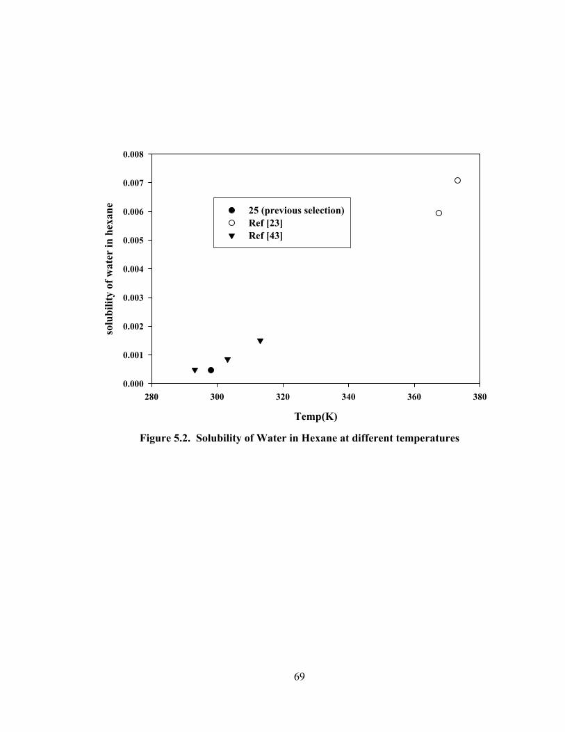
69

Temp(K)

280 300 320 340 360 380

solu

bilit

y of

wat

er in

hex

ane

0.000

0.001

0.002

0.003

0.004

0.005

0.006

0.007

0.008

25 (previous selection)Ref [23]Ref [43]

Figure 5.2. Solubility of Water in Hexane at different temperatures

70

Table 5.1. Parameters of Daubert and Danner [56], Harvey and Lemon [77]

Parameter

of

Ref [56]

LiV sat

ip parameter of

Ref [77]

Bi

Hexane Butanol Hexane Butanol i Water

ai bi A

B

C

D

E

.7147

.265

507.43

.2781

0.

.9677

.26674

562.93

.2457

0.

165.47

-8353.3

-23.972

.02949

1.0

96.23

-9214.3

-10.295

.000002

2.0

1

2

3

4

.34

-.76

-24.22

-3978.2

-0.5

-0.8

-3.35

-8.3

71

Temp(K)

280 300 320 340 360 380

solu

bilit

y of

wat

er in

but

anol

0.48

0.50

0.52

0.54

0.56

0.58

0.60

0.62

0.64

0.66

25(previous selection)Ref [24]Ref [43]Ref [43]

Figure 5.3. Solubility of Water in Butanol at different temperatures

72

temp(K)

260 280 300 320 340 360

solu

bilit

y of

but

anol

in w

ater

0.010

0.012

0.014

0.016

0.018

0.020

0.022

0.024

0.026

0.028

0.030

25 (previous selection)Ref [36]Ref [43]Ref [43]

Figure 5.4. Solubility of Butanol in Water at different temperatures

73

temp(K)

280 300 320 340 360 380

infin

ite d

ilutio

n of

act

ivity

coe

ffic

ient

of

w

ater

in b

utan

ol

2.5

3.0

3.5

4.0

4.5

5.0

5.5

25 (previous selection)Ref [63]Ref [38]Ref [80]

Figure 5.5. Infinite dilution activity coefficient of Water in Butanol at different

temperatures

74

temp(K)

260 280 300 320 340 360 380

infin

ite d

ilutio

n ac

tivity

coe

ffic

ient

of

b

utan

ol in

wat

er

30

35

40

45

50

55

60

65

70

25(previous selection)Ref [35]Ref [63]Ref [57]

Figure 5.6. Infinite dilution activity coefficient of Butanol in Water at different

temperatures

75

x(water)

0.0 0.2 0.4 0.6 0.8 1.0

HE

(j/m

ol)

-200

0

200

400

600

800

1000

1200

30(Ref [74])30(Ref [74])30(Ref [83])55(Ref [74])75(Ref [74])

Figure 5.7. Excess Enthalpy of Water-Butanol at different temperatures

Table 5.2. Coefficients for use in Barker’s method in Equations 2.23 and 2.24

T(K) A0 A1 A2 B1 288.15 293.15 298.15 303.15 308.15 313.15 318.15 323.15

1.8698 1.8553 1.8374 1.8204 1.8049 1.788 1.7741 1.7538

-1.1973 -1.1564

-1.108 -1.1015 -1.0658 -1.0416 -1.0031

-.9645

-.0527 -.0348 -.0234

-.031 -.0182

-.031 .0118 .0163

-.8453 -.8254 -.8047 -.8025 -.7852 -.7745 -.7487 -.7305

76

x(Hexane)

0.0 0.2 0.4 0.6 0.8 1.0

HE

(j/m

ol)

0

200

400

600

800

100015(Ref [89])25(Ref [82])25(Ref [82])35(Ref [82])45(Ref [82])

Figure 5.8. Excess Enthalpy of Hexane-Butanol

77

T(K)

295 300 305 310 315 320 325

infin

ite d

ilutio

n ac

tivity

coe

ffic

ient

of h

exan

e

5.0

5.1

5.2

5.3

5.4

5.5

5.6

5.7

25(previous selection)Ref [65]

Figure 5.9. γ∞ of Hexane-Butanol at different temperatures

78

temp(K)

290 300 310 320 330 340 350

infin

ite d

ilutio

n ac

tivity

coe

ffic

ient

of

but

anol

in h

exan

e

10

20

30

40

50

25(previous selection)Ref [41]

Figure 5.10. γ∞ of Hexane-Butanol at different temperature

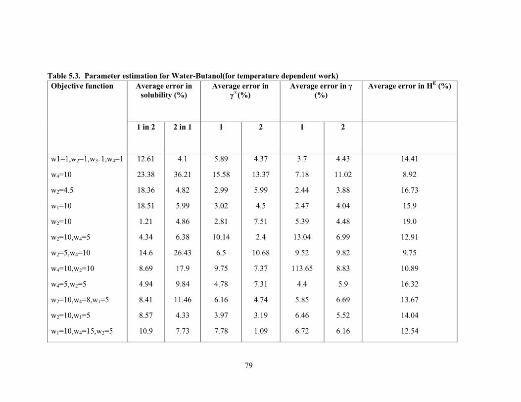
79

Table 5.3. Parameter estimation for Water-Butanol(for temperature dependent work)

Objective function Average error in solubility (%)

Average error in γ∞(%)

Average error in γ (%)

Average error in HE (%)

1 in 2 2 in 1 1 2 1 2

w1=1,w2=1,w3=1,w4=1

w4=10

w2=4.5

w1=10

w2=10

w2=10,w4=5

w2=5,w4=10

w4=10,w2=10

w4=5,w2=5

w2=10,w4=8,w1=5

w2=10,w1=5

w1=10,w4=15,w2=5

12.61

23.38

18.36

18.51

1.21

4.34

14.6

8.69

4.94

8.41

8.57

10.9

4.1

36.21

4.82

5.99

4.86

6.38

26.43

17.9

9.84

11.46

4.33

7.73

5.89

15.58

2.99

3.02

2.81

10.14

6.5

9.75

4.78

6.16

3.97

7.78

4.37

13.37

5.99

4.5

7.51

2.4

10.68

7.37

7.31

4.74

3.19

1.09

3.7

7.18

2.44

2.47

5.39

13.04

9.52

113.65

4.4

5.85

6.46

6.72

4.43

11.02

3.88

4.04

4.48

6.99

9.82

8.83

5.9

6.69

5.52

6.16

14.41

8.92

16.73

15.9

19.0

12.91

9.75

10.89

16.32

13.67

14.04

12.54

80

Table 5.4. Parameter estimation for Hexane-Butanol(for temperature dependent work)

*** objective function for our final parameters.

Objective function Average error in HE

Average error in γ∞(%)

Average error in γ (%)

1

2

1 2

w2=1,w3=1,w4=1

w2=2

w3=3

w4=5

w2=2, w4=5

w2=5, w4=5

w2=2.5,w4=5***

8.95

7.48

6.42

6.05

9.18

8.82

8.53

10.02

11.7

12.39

12.43

9.48

10.31

11.02

14.08

15.51

17.14

11.49

13.69

12.97

12.13

3.41

3.83

4.06

4.33

2.48

2.73

2.57

5.17

6.19

6.93

7.64

3.51

3.85

3.52

81

Table 5.5. Calculated results by NRTL using best fitted parameters (temperature dependent function) for all three pairs

Table 5.6. Best fitted parameters for all three pairs (for temperature dependent work)

Hexane- Water

Water- Butanol

Hexane- Butanol

1.13

5.52

5.49

12.48

8.47

11.02

8.98

2.13

3.14

2.57

6.49

3.52

12.21

8.53

1.2, 1.45/ 1.45

Pair(i-j) A B C α

Hexane-Water i,j

j,i

3381.24

2013.85

7.478

-17.886

-.0167

.1527

.22

Water-Butanol i,j

j,i

1031.46

229.43

6.315

.585

.00096

-.0387

.41

Hexane-Butanol i,j

j,i

910.21

323.42

-.307

-2.157

-.003

.018

.55

82

Hexane0.0 0.1 0.2 0.3 0.4 0.5 0.6 0.7 0.8 0.9 1.0

Butanol

0.0

0.1

0.2

0.3

0.4

0.5

0.6

0.7

0.8

0.9

1.0

Water

0.0

0.1

0.2

0.3

0.4

0.5

0.6

0.7

0.8

0.9

1.0

exp (L1 phase)exp ( L2 phase)25 (L1 phase)25 (L2 phase)40 (L1 phase)40 (L2 phase)60 (L1 phase)60 (L2 phase)75 (L1 phase)75 (L2 phase)

Figure 5.11. Ternary diagram for Hexane-Butanol-Water at higher temperatures

83

mole fraction of butanol in feed

0.0 0.1 0.2 0.3 0.4 0.5 0.6

mol

e fr

actio

n of

but

anol

in L

1 pha

se

0.0

0.1

0.2

0.3

0.4

0.5

0.6

Ref 22Ref 125406075

Figure 5.12. Variation of Butanol concentration in L1 phase at higher temperatures

84

CHAPTER 6

DISCUSSION

Throughout this work, it was observed that careful selection of data and

regression of parameters using x vs. γ data generated from VLE, all γ∞, binary mutual

solubility (LLE) and excess enthalpy data (HE) data made it possible to obtain a universal

liquid state model as well as a universal set of parameters for 25 °C and also for a

temperature range of 10-100 °C. These parameters are not only able to predict binary data

but also ternary data very well. For the Hexane-Water and Water-Butanol pairs, either

two parameter or three-parameter models provide good results. The Hexane-Water pair

does not show any problems due to the fact that the solubility itself is in infinite dilution

and appropriate γ∞ values can be obtained using any model. Also, problems do not arise

for the Water-Butanol pair since they are partially miscible and the x-γ functionality

change within the miscibility gap is not known and cannot be described by any of the

models. For these Hexane-Water and Water-Butanol pairs, any of the models can be used

to fit the data at infinite dilution and finite concentration simultaneously. These two pairs

did not show large deviations between calculated and experimental data. However, it was

not possible to fit the data for all concentration ranges for the Hexane-Butanol pair. From

x-γ analysis, it was found that at dilute concentrations γ values of Butanol increases very

sharply. So any model which can represent sharp functionality changes can only be able

to fit the data of this pair. The two-parameter models were found unable to show rapid

changes of x-γ values. For the other two pairs, since γ changes smoothly with

concentration, the two-parameter models perform well. Three-parameter models are

capable of showing steep γ changes. The third additional parameter (in terms of non-

randomness) helps to adjust the fit. It is also very important that the three-parameter

models can only fit the data when the third parameter is regressed independently.

Otherwise, there would be no difference between the three and two-parameter models.

This additional parameter has the flexibility to fit the data for all concentration ranges. As

seen in Figure 4.13, using the three-parameter models to fit the data showed the same

85

behavior as in the UNIQUAC or LSG model. This is due to the fact that the third

parameters were kept fixed and other two interaction parameters were regressed.

For ternary systems, using the three-parameter models is not straightforward. Due

to the immiscible pair, Hexane-Water, many combinations of third parameters and binary

parameters are possible. Although every combination will give reasonable solubility

values for this binary pair, they will not necessarily give good ternary results. The Water-

rich phase calculations can be done using any set of parameters, unlike the Hexane-rich

phase. In the Water-rich phase, the amount of Hexane and Water remain nearly fixed

throughout the entire concentration range. In the Hexane-rich phase, as the Butanol

concentration increases, the concentration of Hexane and Butanol changes substantially.

Hence, different third parameters will give different results for this phase. The most

accurate way of selecting suitable third parameters is to compare the calculated results

with the experimental data, which is very tedious work. As seen from the results,

optimum ternary data can be achieved at α=.22 (NRTL) and λ=254 (GEM-RS) after a

thorough investigation with this third parameter.

Following the same procedures of the work at 25 °C, it is also possible to acquire

a single set of parameters for the temperature range between 10 and 100 °C. In addition

to phase equilibrium calculations, excess enthalpy data can be reasonably predicted with

these parameters, all within fair error.

86

CHAPTER 7

CONCLUSION

From our observations the following conclusions can be drawn:

Data selections should be done very cautiously.

Hexane-Butanol pair was the main problem for fitting data since x-γ shows steep

function.

Two-parameter models can not fit this steep function; however, three-parameter

models can represent that.

Regression has to be done using all kinds of possible data.

The Third parameter has to be regressed independently.

Selecting the appropriate third parameter of three parameter model for an

immiscible pair (Hexane-water) is very important since only a fixed α or λ of

NRTL and GEM-RS are able to predict ternary data well.

From our results it is observed that, NRTL/GEM-RS (three-parameter models) are

the universal models for Hexane-Butanol-Water system because these models can

fit the data for Hexane-Butanol pair which show sharp x-γ change,

predict all kinds of binary phase equilibrium data,

represent ternary data from very dilute region to finite concentration

simultaneously, and

calculate Dsw correctly.

Hence, it is possible to obtain universal liquid mixture models for VLE and LLE,

meaning that separate sets of parameters are not needed to calculate different types of

phase equilibrium data. The work based on a typical non-ideal ternary system that is

Hexane-Butanol-Water was satisfactory. However, more work is needed to be done to

show that this process provides acceptable universal parameters for other non-ideal

ternary systems like Benzene-Methanol-Water, Hexane-Propanol-Water and so on. This

process can be further validated if used on quaternary systems.

87

REFERENCES

[1] Javvadi, A. Partitioning of Higher Alcohols in Alkane-Water at Dilute

Concentrations, MS Thesis, 2000. North Carolina A&T State University.

[2] Prausnitz, J.M.; Lichtenthaler, R. N.; Azevedo, E.G. Molecular thermodynamics

for fluid phase equilibria. Prentice Hall International Series in the Physical and

Chemical Engineering Sciences. Third Edition,2005

[3] Vera, J.H.; Sayegh, S.G.; Ratcliff, G.A. A Quasi Lattice-Local Composition Model

for the Excess Gibbs free energy of Liquid Mixtures. Fluid Phase Equilibria

1977,1,113

[4] Renon, H.; Prausnitz, J.M. Local Compositions in Thermodynamic Excess

Functions for Liquid Mixtures. AIChE Journal. 1968, 14, 135

[5] Abrams, D. S.; Prausnitz, J. M. Statistical Thermodynamics of liquid Mixtures: A

New Expression for the Excess Gibbs energy of Partly or Completely Miscible

systems. AIChE Journal, 1975, 116

[6] Maurer. G.; Praunirz. J.M. On the Derivation and extension of uniquac equation.

Fluid Phase Equilibria.1978,2, 91

[7] Anderson, T. F.; Prausnitz, J. M. Appication of the Uniquac Equation to Calculation

of Multicomponent Phase Equilibria. 2. Liquid-Liquid Equilibria Ind. Eng. Chem.,

Process Des. Dev., 1978, 17, 561

[8] Nagata, I.; Katoh, K. Effective UNIQUAC Equation in Phase Equilibrium

Calculation. Fluid Phase Equilibria, 1981, 5, 225.

[9] Larsen. B. L.; Ramussen. P; Fredenslund. A. A Modified UNIFAC Group-

Contribution Model for Prediction of Phase Equilibria and Heats of Mixing. Ind.

Eng. Chem. Res. 1987, 26, 2274

[10] Weidlich. U.; Gmehling. J. A Modified UNIFAC Model. 1. Prediction of VLE, hE,

and γ∞. Ind. Eng. Chem. Res. 1987, 26, 1372

[11] Nagata. I. Modification of the Extended Uniquac Model for Ternary and Quaternary

Liquid-Liquid Equilibrium Calculations. Fluid Phase Equilibria, 1989, 51, 53

88

[12] Tamura. K.; Chen. Y.; Tada. K.; Yamada. T.; Yamada. T.; Nagata. I.;

Representation of Multicomponent Liquid-Liquid Equilibria for aqueous and

Organic Solutions Using a Modified UNIQUAC Model. Journal of Solution

Chemistry. 2000,29, 463

[13] Tse, G.; Sandler, S. I. Determination of Infinite Dilution Activity Coefficients and

1-Octanol/Water Partition Coefficients of Volatile Organic Pollutants. J. Chem.

Eng. Data, 1994, 39, 354

[14] P. Alessi, M.; Fermeglia, M.; Kikic, I. Significance of Dilute Regions. Fluid

Phase Equilibria, 1991,70,239

[15] Chapoy, A.; Haghighi, H.; Tohidi, B. Development of a Henry’s constant

correlation and solubility measurements of n-pentane, I pentane, Cyclopentane,n

hexane, and toluene in water. J. Chem. Therm, 2008, 40, 1030

[16] Macauliffe, C. Solubility in Water of C1-C9 Hyderocarbon.Nature (London). 1963,

200,1092

[17] Polak J.; B.C. Lu. Mutual Solubilities of Hydrocarbons and Water at 0 and 25 C.

Can. J. Chem. 1973,51,4018

[18] Leinonen, P.J.; Mackay. D. The Multicomponent Solubility of Hydrocarbons in

Water. Can. J. Chem. 1973,51,230

[19] Mackay, D.; Shiu, W.Y. A Critical Review of Henry’s Law Constants for

Chemicals and Environmental Interest. J. Phys. Chem. Ref. Data. 1981,10,1175

[20] Tsonopoulos, C.; Wilson, G.M. High Temperature Mutual Solubilities of

hydrocarbons and Water .AIChE Journal. 1983, 29, 990

[21] Deal, C. H.; Derr, E. L. Selectivity and Solvency in Aromatics Recovery. Ind.

Eng. Chem. Process Des. Dev. 1964,3, 394

[22] Sugi, H.; Katayama, T. Liquid-Liquid Equilibrium Data for Three Ternary Systems

of Aquous Alcohol Solutions and Applicability of The Analytical Solutions of

Groups.J. Chem. Eng. Jpn. 1977,10, 400

[23] Roddy, J. W.; Coleman, C. F. Solubility of Water in Hydrocarbons as a Function of

Water Activity. Talanta. 1968, 15,1281

89

[24] Hill, A.E. ; Malisoff, W. M. The Mutual Solubility of Liquids. III. The Mutual

Solubility of Phenol and Water . IV. The Mutual Solubility of Normal Butyl

Alcohol and Water. J. Am. Chem. Soc 1926,48,918

[25] Kinoshita, K. ; Ishikawa, H.; Shinoda, K. Solubility of Alcohols in Water

Determined by the Surface Tension Measurements. Chem. Soc. Jpn. 1958,31, 1081

[26] Yaws, C.L.; Hopper, J.R.; Sheth, S.D.; Hen, M.; Pike, R.W. Solubility and Henry’s

Law Constant for Alcohols in Water. Waste Management.1997, 17,541

[27] Lebert, A.; Richon, D. Infinite Dilution Activity Coefficients of N-Alcohols as a

function of Dextrin Concentration in Water-Dextrin Systems.J. Agri. Food

Chem.1984,32,1156

[28] Mash, C.J.; Pemberton, R.C. Activity Coefficient at very low concentrations for

organic solutes in Water determined by an Automatic Chromatographic Method.

NPL Report Chem. 111 Natl Phys. Lab., Middlesex., U.K., July 1980.

[29] Rytting, J.H.; Huston, L.P.; Higuchi, L.P. Thermodynamic Group Contributions

for Hydroxyl, Amino, and Methyl Groups. J. Pharm. Sci 1978,67,615

[30] Landau, L.; Belfer, A.J; Locke, D.C. Measurements of Limiting Activity

Coefficients Using Non-Steady State Gas Chromatography. Ind. Eng. Chem.

Res.1991,30,1900

[31] Djerki, R.A.; Laub, R.J. Solute Retention in Column Liquid Chromatography. X.

Determination of Solute Infinite-Dilution Activity Coefficients in Methanol, Water,

and Their Mixtures by Combined Gas-Liquid and Liquid-Liquid Chromatography.

J. Liquid Chromatgr.1988,11, 585

[32] Li. J.J.; Carr, P.W. Measurement of Water-Hexadecane Partition Coefficients by

Headspace Gas Chromatography and Calculaton of Limiting Activity Coefficients

in Water. Anal. Chem. 1993,65,1443

[33] Abraham, M.H.; Whitting, G.S; Fuchs, R.; Chambers, E.J. Thermodynamics of

Solute Transfer from Water to Hexadecane. J. Chem. Soc., Perkin Trans.1990,2,

291

90

[34] Paul, G.W.; Sandler,S.I. Headspace gas chromatography for measurement of

infinite dilution activity coefficients of C4 alcohols in water. Fluid Phase

Equilibria. 1999,157,111

[35] Vrbka, P.; Fenclova, D.; Lastovka, V.; Dohnal, V. Measuremnt of inifinite dilution

activity coefficients of 1-alkanols (C1-C5) in water as a function of temperature

(273-373 K). Fluid Phase Equilibria 2005,237, 123

[36] Hill, A.E.; Malisoff, W. M. The Mutual Solubility of Liquids. III. The Mutual

Solubility of Phenol and Water. IV. The Mutual Solubility of Normal Butyl Alcohol

and Water. J. Am. Chem. Soc 1926,48,918

[37] Petrisis V.E.; Geankoplis C.J. Phase Equilibria in 1-Butanol-Water-Lactic Acid

System. J. Chem. Eng. Data 1959,4,197

[38] Pierotti G. J.; Deal C.H.,Derr E.L. Activity Coefficients and Molecular Structures.

Ind. Eng. Chem. 1959,51,95

[39] Gmehling J.; Menke J.; Schiller, M. Activity Coefficients at infinite dilution.

Chemistry Data Series, Vol. IX, Part 4, 1994

[40] Castells C.B.;Carr. P.W.; Eikens D.I.; Bush D. Comparative Study of

Semitheoritical Models for Predicting Infinite Dilution Activity Coefficients of

Alkanes in Organic Solvents. Ind. Eng. Chem. Res. 1999,38,4104

[41] Thomas, E. R.; Newman, B.A.; Long, T.C.; Wood, D.A.; Eckert, C.A. Limiting

Activity Coefficients of Polar and non polar solutes in both volatile and non

volatile solvents by Gas Chromatography. J. Chem. Eng. Data 1982, 27,399

[42] Thomas, E. R.; Newman, B.A.; Nicolaides, G. L.; Eckert C.A.; Limiting Activity

Coefficients from Differential Ebulliometry. J. Chem. Eng. Data 1982, 27,233

[43] Ghemehling, G.; Onken U. Vapor Liquid Equilibrium Data Collection.

DECHEMA, Chemistry Data Series,Vol 1. Part 1, 1977

[44] Sorensen J. M.; Arlt W. Liquid-Liquid Equilibrium Data Collection. DECHEMA,

Chemistry Data Series, 1979, Vol V,Part 1

[45] Thomas, E. R.;Newman, B.A.; Nicolaides, G. L.; Eckert C.A. Limiting Activity

Coefficients from Differential Ebulliometry. J. Chem. Eng. Data 1982, 27,233

91

[46] Reid, R.C.; Prausnitz, J.M.; Polling, B.E. The properties of Gases And Liquids.

McGraw Hill, New-York, 4th ed.,1987

[47] Rodriguez, V.; Pardo, J.; Lopez, M.C.; Royo, F.M.; Urieta, J.S. Vapor Pressures

of Binary Mixtures of Hexane+1 Butanol,+2 butanol,+2 Methyl 1 Propanol, or+ 2

Methyl 2 Propanol at 298.15 K. J. Chem. Eng. Data 1993,38,350

[48] Gracia, M.; Sanchez, F.;Perez, P;Valero, J.; Losa, C.G. Vapor Pressure of (butan-1

ol+hexane) at temperatures between 283.1 and 323.12 K. J. Chem. Therm 1992, 24,

463

[49] Garriza, R.; Mertinez, S.; Perez, P.; Gracia,M. Vapor Pressure at Several

Temperatures between 278.15 and 323.15 K and Excess Functions at T=298.15 for

1 Bromobutane with 1 Butanol or 2 Methyl-2-propanol. J. Chem.Eng.Data 2002,

47, 322

[50] Ambrose D.; Ghiasse, N.B. Vapor pressure and critical temperatures of some

alkanoic acids; C1 to C10. J. Chem. Therm. 1987, 19, 505-519

[51] Hansch, C.; Leo, A. Substituent Constants for Correlation analysis in Chemistry and

Biology. Wiley – Interscience, NY, 1979

[52] Barker, J.A. Determination of Activity Coefficients from Total Pressure

Measurements. Aust. J. chem.1953,6,207

[53] ASME Steam Tables. American Society of Mechanical Engineers, NY, 1993.

[54] Selected Values of Chemicals Compounds. TRC Tables. Thermodynamic Research

Center Data Project, College Station, TX,1995

[55] Dymond, J.H.; Marsh, K.N.; Wilhoit, R.C. Virial Coefficients of Pure Gases and

Mixtures. Group IV: Volume 21,Springer,2003

[56] Daubert, T.E.; Danner, R. P. Physical and Thermodynamic Properties of Pure

Chemicals. Data Compilation. Part 2 &3, Taylor & Francis, 1992

[57] Gmehling J.; Menke J. Activity Coefficients at Infinite Dilution.Chemistry Data

Series, Vol. IX, Part 4

[58] Gmehling, J; Menke J. Activity Coefficients at infinite dilution, C1-C16.

DECHEMA, Chemistry Data Series, 2007, Vol IX, Part 5

92

[59] Tsonopoulos, C. An Empirical Correlation of Second Virial Coefficients. AIChE

Journal, 20, 263

[60] Tarakad, R.R.; Danner, R.P. An Improved Corresponding States Method for Polar

Fluids: Correlation of Second Virial Coefficients. AIChE J.1977,23,685

[61] Lin, S.T.; Sandler, S. I. Prediction of Octanol-Water Partition Coefficients Using a

Group Contributoion Solvation Model. Ind. Eng. Chem. Res, 1999, 38,4081

[62] Lin, S.T.; Sandler, S. I. A Priori Equilibrium Prediction from a Segment

Contribution Solvation Model. Ind. Eng. Chem. Res, 2002, 41,899

[63] Tochigi, K.; Tiegs, D.; Gmheling, K.; Kojima, K. Determination of New ASOG

Parameters. J.Chem.Eng.Japan,1990,23,453

[64] Li, J.; Carr, P.W. Gas chromatographic study of salvation enthalpy by

solvatochromically based linear salvation energy relationships. J. Chrom,

1994,659,367

[65] Dobrjakov, Y.G.; Balashova, I.M.; Maurer, G. The limiting activity coefficient of

phenol in Water and Some organic solvents from Differential Ebuliometry. Fluid

Phase Equilibria. 2001,181,59

[66] Gmehling, J.; Mollmann, C. Synthesis of Distillation Process using Thermodynamic

Models and the Dortmund Data Bank. Ind.Eng.Chem.Res. 1988,37,3112

[67] McCann, D.W.; Danner, R.P. Prediction of Second Virial Coefficients of Organic

compounds by a Group Contribution Method. Ind.Eng.Chem.Process Des.Dev.

1984,23,529

[68] Vetere, A. On the Calculation of the Second Virial Coefficients of Pure Compound

And Mixture. Chem.Eng.Sci.1991,46,1787

[69] Hendi, H.; Vogel, E. Second Cross Virial coefficient of the Binary Vapor Mixture

n-Hexane/Methanol from Quasi-isochoric ppT Measurements. Fluid Phase

Equilibria. 1996,125,55

[70] Vetere, A. An Improved Method to Predict Second Cross Virial Coefficients. Fluid

Phase Equilibria. 2005,230,15

93

[71] Ghemehling G.; Onken U. ; Arlt W. Vapor Liquid Equilibrium Data Collection.

DECHEMA, Chemistry Data Series,Vol 1. Part 1a, 1981

[72] Ghemehling G.; Onken U.; Rarey-Nies, J.R. Vapor Liquid Equilibrium Data

Collection. DECHEMA, Chemistry Data Series, Vol 1. Part 1b, 1987

[73] Sorensen J. M.; Arlt W. Liquid-Liquid Equilibrium Data Collection. DECHEMA,

Chemistry Data Series, 1980, Vol V,Part 2-3

[74] Christensen, C.; Gmehling, J.; Rasmussen, P.; Weidlich, U. Heats of Mixing Data

Collection, Binary System. Chemistry Data series. 1984, Vol 3,part 1.

[75] Kojima, K.; Zhang, S; Hiaki, T. Measuring Methods of Infinite Dilution Activity

Coefficients and a Database for Systems Including Water. Fluid Phase Equilibria,

1997,131,145

[76] Ghemehling G.; Onken U. Vapor Liquid Equilibrium Data Collection. DECHEMA,

Chemistry Data Series,Vol 1. Part 1c, 2003

[77] Harvey, A. H.; Lemon, E.W. Correlation for the Second Virial Coefficient of

Water. J. Phys. Chem. Ref. Data. 33, 369,2004

[78] Fischer, K.; Gmehling, J. P-x and γ∞ Data for the Different Binary Butanol-Water

systems at 500 C. J. Chem. Eng. Data. 1994, 39, 309

[79] Butler, J.A.V.; Thomson, D.W.; Maclennan, W.H. The Free Energy of the Normal

Alcohols in Aqueous Solution. Part I. The Partial Vapor Pressures of Aqueous

Solutions of Methyl, n-Propyl, and n-Butyl Alcohols. Part II. The Solubilities of

Some Normal Aliphatic Alcohols in Water. Part III. The Theory of Binary

Solutions, and its Application to Aqueous-Alcoholic Solutions. J. Chem.

Soc(London) 1933, 674

[80] Loblein, G.M.; Prausnitz, J.M. Infinite Dilution Activity Coefficients from

Differential Ebulliometry. Ind.Eng.Chem.Fundum.1982,21,109

[81] Tochigi, K.; Kojima, K. The Determination of Group Wilson Parameters to Activity

Coefficients by Ebulliometer. J.Chem.eng.Jpn. 1976,9,267

[82] Christensen, C.; Gmehling, J; Rasmussen, P.; Weidlich, U. Heats of Mixing Data

Collection, Binary System. Chemistry Data series. Vol 3,part 1.1984

94

[83] Goodwin, S.R.; Newsham, D.M. A flow calorimeter for the determination of

enthalpies of mixing of liquids: enthalpies of mixing of water+n-propanol and

water+n butanol at 300 C. J. Chem. Thermodyn.1971,3,325

[84] Berro, C.; Rogalski, M.; Peneloux, A. Excess Gibbs Energies and excess volumes

of 1 -Butanol-n-Hexane and 2-methyl-1-propanol-n-Hexane binary systems.

J.Chem.Eng.Dat.1982,27,352

[85] Regina, M.W.; Maciel, A.Z.F. Vapor-Liquid phase equilibrium measurements for

the n-hexane-1-butanol system at 323.15, 338.15 and 348.15 K. Fluid Phase

Equilibria.1989,50,201

[86] Castells C.B.; Carr. P.W; Eikens D.I.; Bush D. Comparative Study of

Semitheoritical Models for Predicting Infinite Dilution Activity Coefficients of

Alkanes in Organic Solvents. Ind. Eng. Chem. Res. 1999,38,4104

[87] Thomas, E.R.; Newman, B.A.; Long, T.C.; Wood, D.A.;Eckert, C.A. Limiting

Activity Coefficients of Polar and non polar solutes in both volatile and non volatile

solvents by Gas Chromatography. J. Chem. Eng. Data. 1982, 27,39

[88] Arlt, W.;Sphul, O.; Klamt, A. Challenges of Thermodynamics. Chemical

Engineering and Proceeding.2004,43,221

[89] Nguyen, T.H.; Ratcliff, G, A. Heats of Mixing of n-Alcohol-n-Alkane Systems at15

and 55 C. J.Chem.Eng.Data.1975,20,252

[90] Introduction of Chemical Engineering Thermodynamics. Smith, J.M; Van Ness,

H.C; Abbot, M.M. 5th edition. McGraw-Hill International Editions, 1996.

[91] Abbot, M., M.; Low pressure phase equilibria: Measurement of VLE, Fluid Phase

Equilib, 1986,29, 193

[92] Rarey, J., R.; Gmehling, J. Computer-operated static apparatus for the

measurement of vapor-liquid equilibrium data, Fluid Phase Equilib. 1993,83, 279

[93] Malanowski S.; Experimental methods for vapour-liquid equilibria. II. Dew- and

bubble-point method, Fluid Phase Equilib. 1982,9,311

95

APPENDIX A

DERIVATION OF EQUATION IN CHAPTER 3

Here, the thermodynamic relations to derive Equation 3.3 (in Chapter 3) are

shown. This technique is based on no assumptions concerning liquid-phase nonideality

other than the obvious one of the finiteness of the activity coefficient and of its

composition derivative at infinite dilution. The fugacity coefficient terms, not too critical

at the atmospheric or lower pressure used here, are obtained from virial coefficients.

At equilibrium,

0 01 1 1 1 1 1L L V Vx f y fγ γ= =>

01 11

01 1 1

VL

V L

y fx f

γγ

=

(A1)

as x1 approaches zero, the right hand side approaches form 0/0. Applying L’ Hospital’s

rule yields

1 1 1

0 01 11 1

10 01 1 1 10 0 0

V VL

V L Lx x x

f fy Kx f f

γγ

= = =

⎡ ⎤ ⎡ ⎤⎛ ⎞ ⎛ ⎞⎛ ⎞ ⎛ ⎞∂= =⎢ ⎥ ⎢ ⎥⎜ ⎟ ⎜ ⎟⎜ ⎟ ⎜ ⎟∂⎝ ⎠⎝ ⎠ ⎝ ⎠⎝ ⎠ ⎣ ⎦ ⎣ ⎦

(A2)

Here K is the equilibrium vaporization ratio. An equation for component 2 analogous to

equation (A2) becomes

y1=1-y2= 0

2 2 2 2 20

2 2

oV V L L

V V

f x ff

γ γγ−

(A3)

Differentiating with respect to x1 and noting that x1=0, γ2V=γ2L=1.0, f2L0=f2V

0=f20

96

( )

( )

1 1

1

0 02 20

20 01 1

2 1 20 01 1 2 20 0

0

1 1

V L

V Lx x

x

f ff

y xf x fx x f f

= =

=

⎡ ⎤∂ −+⎢ ⎥

⎛ ⎞ ⎧ ⎫∂ ∂∂ ⎢ ⎥⎡ ⎤= − − =⎨ ⎬⎜ ⎟ ⎣ ⎦ ⎢ ⎥∂ ∂⎝ ⎠ ⎩ ⎭ ⎢ ⎥⎢ ⎥⎣ ⎦

(A4)

This equation is applicable to both constant pressure and constant temperature data

At constant pressure,

( ) ( )0 0 0 02 2 2 2

1 1

V L V L

PP P

f f f f Tx T x

⎡ ⎤ ⎡ ⎤∂ − ∂ − ⎛ ⎞∂⎢ ⎥ ⎢ ⎥= ⎜ ⎟∂ ∂ ∂⎢ ⎥ ⎢ ⎥ ⎝ ⎠⎣ ⎦ ⎣ ⎦

(A5)

here 1

Tx

⎛ ⎞∂⎜ ⎟∂⎝ ⎠

is the slope of an isobaric temperature-liquid composition curve.

now,

( )2

0 22 2 2,

exp (A6)satsat satL

L P T

Vf P PRT

ϕ π⎡ ⎤= −⎢ ⎥⎣ ⎦

( )2

0 22 , 2 2,

exp (A7)satsat satV

V P T P T

Vf P P PRT

ϕ ϕ ⎡ ⎤= = −⎢ ⎥⎣ ⎦

( ) ( )

( ) ( ) ( ) (A8) exp

expexp

22222

2222,2

,222

222,

02

2

2

2

⎥⎥⎦

⎤

⎢⎢⎣

⎡⎟⎟⎠

⎞⎜⎜⎝

⎛∂∂

−⎟⎠⎞

⎜⎝⎛∂∂−

+−

−−

+⎟⎟⎠

⎞⎜⎜⎝

⎛

∂

∂−+⎟⎟

⎠

⎞⎜⎜⎝

⎛∂∂−

=⎟⎟⎠

⎞⎜⎜⎝

⎛∂∂

π

πππ

ϕ

ϕϕ

TP

RTV

TV

RTPP

RTPPV

RTPPVP

TRTPPVP

TP

RTPPV

Tf

satL

P

Lsatsat

Lsat

LTP

sat

TPsat

Lsatsatsat

LTP

L

sat

sat

sat

( ) ( )

( ) ( ) ( )(A9) exp

expexp

22222

2222,2

,222

222,

02

2

2

2

⎥⎥⎦

⎤

⎢⎢⎣

⎡⎟⎟⎠

⎞⎜⎜⎝

⎛∂∂

−⎟⎠⎞

⎜⎝⎛∂∂−

+−

−−

+⎟⎟⎠

⎞⎜⎜⎝

⎛

∂

∂−+⎟⎟

⎠

⎞⎜⎜⎝

⎛∂∂−

=⎟⎟⎠

⎞⎜⎜⎝

⎛∂∂

P

satV

P

Vsatsat

Vsat

VTP

sat

TPsat

Vsatsatsat

VTP

V

TP

RTV

TV

RTPP

RTPPV

RTPPV

P

TRTPPV

PT

PRT

PPVT

f

sat

sat

sat

ϕ

ϕϕ

πππ

now, at x1=0, we assume that,P2sat≈ P ≈ f2

0 and Φ P2sat

,T ≈ 1

97

so, from equation (A6) and (A7)

( )(A10) 222

2

02

02 ⎟

⎠⎞

⎜⎝⎛ −⎟⎟

⎠

⎞⎜⎜⎝

⎛∂∂

−=⎥⎦

⎤⎢⎣

⎡∂−∂

RTV

RTV

TPP

Tff LV

satsatLV

ππ

(A11) 222

2

2 ⎟⎠⎞

⎜⎝⎛ −⎟⎟

⎠

⎞⎜⎜⎝

⎛∂∂

−=RTV

RTV

TP

PP LV

P

sat

sat

sat

⎟⎠⎞

⎜⎝⎛ −⎟⎟

⎠

⎞⎜⎜⎝

⎛−=

RTPV

RTPV

dTPdf LV

sat2220

2ln

π (A12)

from Eq. (A4) we get that,

( )1

0 02 2 0 22 2

21 1

, 0

ln satV L V L

P x

f f PVd P PVTfx x dT RT RT

π=

⎡ ⎤∂ − ⎛ ⎞ ⎛ ⎞∂ ⎛ ⎞⎢ ⎥ = − −⎜ ⎟ ⎜ ⎟⎜ ⎟∂ ∂ ⎝ ⎠⎢ ⎥ ⎝ ⎠⎝ ⎠⎣ ⎦

(A13)

combining eqn (A2), (A4) and (A9)

1

01 21 2 20

1 1 10

ln1 (A14)sat

V VL L

V L Px

f PVd P PVTf x dT RT RT

γγ

=

⎡ ⎤⎧ ⎫⎛ ⎞ ⎛ ⎞ ⎛ ⎞∂⎪ ⎪ ⎛ ⎞= − −⎢ ⎥⎨ ⎬⎜ ⎟ ⎜ ⎟ ⎜ ⎟⎜ ⎟∂ ⎝ ⎠⎪ ⎪ ⎢ ⎥⎝ ⎠⎝ ⎠⎝ ⎠⎩ ⎭ ⎣ ⎦

Now, for low pressure equations

Assumptions:

1

010

1 1

2

1

1

V

vsat

L

V

f P

f PPVRT

γ ≈

≈

≈

≈

( )1

01 1 2

1 001 1

ln1 (A15)sat

V Vx

L P

f d PTf x dT

γγ=

⎡ ⎤⎛ ⎞ ⎛ ⎞∂= −⎢ ⎥⎜ ⎟ ⎜ ⎟∂⎢ ⎥⎝ ⎠⎝ ⎠⎣ ⎦

=> ( )1

21 0

1 1

ln1 1 (A16)sat

satxP

d PP TP x dT

γ=

⎡ ⎤⎛ ⎞ ⎛ ⎞∂= −⎢ ⎥⎜ ⎟ ⎜ ⎟∂⎢ ⎥⎝ ⎠⎝ ⎠⎣ ⎦

98

this is same as equation 3.3 in chapter 3

from equation. (A1),

1

010

1 1

11

1 0

V

L L

V

x

ff

xy

γγ

=

=⎛ ⎞∂⎜ ⎟∂⎝ ⎠

(A17)

( )

1

0 02 20

21 1

01 20

(A18)

V L

x

f ff

y xx f

=

∂ −+

⎛ ⎞∂ ∂=⎜ ⎟∂⎝ ⎠

=

( )1

0 02 20 1

21 1 0

02

(A19)

V L

x

f f yfy x

f=

∂ − ⎛ ⎞∂+ ⎜ ⎟∂ ∂⎝ ⎠

= ( )

1

0 02 21

02 1 10

11 (A20)V L

x

f fyf x y

=

∂ −⎛ ⎞∂+ ⎜ ⎟∂ ∂⎝ ⎠

( )1

0 02 21

01 2 10

11 1 (A21)V L

x

f fyx f y

=

⎧ ⎫∂ −⎛ ⎞∂ ⎪ ⎪⇒ − =⎨ ⎬⎜ ⎟∂ ∂⎝ ⎠ ⎪ ⎪⎩ ⎭

( )

1

10 0

1 2 20 02

10

2

1

V Lx

yx f f

fy

f

=

⎛ ⎞∂⇒ =⎜ ⎟∂ ∂ −⎝ ⎠

−∂

(A22)

at constant pressure,

( ) ( )0 0 0 02 2 2 2

1

(A23)V L V L

PP P

f f f f Ty T y

⎡ ⎤ ⎡ ⎤∂ − ∂ − ⎛ ⎞∂⎢ ⎥ ⎢ ⎥= ⎜ ⎟∂ ∂ ∂⎢ ⎥ ⎢ ⎥ ⎝ ⎠⎣ ⎦ ⎣ ⎦

99

= 0 22 22

ln (A24)sat

V L

PP

PVd P PV TfdT RT RT y

⎛ ⎞ ⎛ ⎞∂⎛ ⎞− −⎜ ⎟ ⎜ ⎟⎜ ⎟ ∂⎝ ⎠⎝ ⎠⎝ ⎠

so, from equations. (A2), (A11) and (A12)

1

0110

1 1 22 20

1

1 (A25)ln1

VLsat

V L V Lx

P

ff PVd P PVT

y dT RT RT

γγ

=

⎛ ⎞=⎜ ⎟ ⎛ ⎞ ⎛ ⎞∂ ⎛ ⎞⎝ ⎠ + −⎜ ⎟ ⎜ ⎟⎜ ⎟∂ ⎝ ⎠⎝ ⎠⎝ ⎠

For low pressure equation considering previous assumptions,

( )1

1 01 2

1

1 (A26)ln1

L satx sat

P

PP d PT

y dT

γ=

⎡ ⎤⎢ ⎥⎢ ⎥= ⎢ ⎥⎛ ⎞ ⎛ ⎞∂+⎢ ⎥⎜ ⎟ ⎜ ⎟∂⎢ ⎥⎝ ⎠⎝ ⎠⎣ ⎦

At constant temperature from equation. A5 we can write,

( ) ( )0 0 0 02 2 2 2

1

V L V L

TT T

f f f f Px P x

⎡ ⎤ ⎡ ⎤∂ − ∂ − ∂⎛ ⎞⎢ ⎥ ⎢ ⎥= ⎜ ⎟∂ ∂ ∂⎝ ⎠⎢ ⎥ ⎢ ⎥⎣ ⎦ ⎣ ⎦

(A27)

Now,

( ) ( )

( ) ( )

2

2

2

0,2 2 2 2

2 2 2,

22 2 2 22 2,

exp exp

exp 1 (A28)

sat

sat

sat

satP T sat sat satL L L

P T

satsatsat satL L L

P T

f V P VP P P P PP P RT P RT

P PV V P VP P PRT RT P RT P

ϕϕ

ϕ

∂∂ ∂⎡ ⎤ ⎡ ⎤= − + −⎢ ⎥ ⎢ ⎥∂ ∂ ∂⎣ ⎦ ⎣ ⎦⎧ ⎫−⎛ ⎞∂ ∂⎪ ⎪⎡ ⎤+ − − +⎨ ⎬⎜ ⎟⎢ ⎥ ∂ ∂⎣ ⎦ ⎝ ⎠⎪ ⎪⎩ ⎭

considering same assumptions

0

2 22 (A29)satL Lf VP

P RT∂

=∂

similarly, 0

2 22 (A30)satV Vf VP

P RT∂

=∂

( )0 0

2 2 02 22 22 2 (A31)V L sat V VL L

T

f f V VV VP fP RT RT RT RT

⎡ ⎤∂ − ⎛ ⎞ ⎛ ⎞⎢ ⎥ = − = −⎜ ⎟ ⎜ ⎟∂ ⎝ ⎠ ⎝ ⎠⎢ ⎥⎣ ⎦

100

APPENDIX B

COMPARISON OF CALCULATED AND EXPERIMENTAL Dsw OF TERNARY

SYSTEMS

In this section, all the ternary systems that were studied from DECHEMA [73] are

listed from Tables B1 to B4. From these tables, it is simple to observe for which systems

the calculated Dsw show good match with literature values and which systems show

significant errors. The first component is the solvent and the second component is the

solute. The first and second columns have the calculated and literature distribution

coefficient, Dsw values using common UNIQUAC parameters.

101

Table B1. Ternary systems with minimum solute concentration in the range of 0≤x≤.01

System Dsw(calc) Dsw(lit) xi (phase 1) xi (phase2) Reference [73], page/vol

Parameters available

1. Benzene-2-Methyl-1-propanol-water

2. Benzene-2-Methyl-2-

propanol-water 3. Nitrobenzene-phenol-

water 4. 1-butanol-3-Methyl 1,3

butanediol-water 5. 1-butanol-succinic acid-

water 6. 2-butanone-2-butanol-

water 7. 2-butanone-1,2,3

propanetricarboxylic acid-water

8. 2-butanone-nicotine-water 9. 1-aza cycloheptane-6

amino lactam hexanoic acid-water

10. Benzene-furfural-water 11. 1-butanol-2 hydroxy

propanoic acid-water 12. Tri chloro ethane-6-amino

3.06

3.07

3.0557

2.7275

2.609

9.807 1.874

1.9928

4.11/ 3.84

1.27/ 1.33

49.91/ 41.51/ 44.48

--

2.67 -- --

-- --

-- 2.2

--

--

--

.00967

.00682

.0009

.003

.00011 .009

.00667

.00281

.00046

.00730

.00213

.00231 .00568

.00317

.00228

.00399

.00002

.002

.00003 .002

.00102

.00296

.00018

.00036 .0011

.00242

.00276

.00093

142/2

143/2

259/3

116/3

11/3 17/3 23/3

31/3 335/3

190/3 533/2

159/2

532/2

59/2

Yes

Yes

No

Yes

Yes Yes No

No No

Yes Yes

Yes

Yes

Yes

102

lactam hexanoic acid-water

13. 2-butanone-2-hydroxy propanoic acid-water

14. 4,4 dimethyl 1,3 dioxane-formic acid-water

15. Tri chloro ethane-6-amino lactam hexanoic acid-water

16. Furfural-formic acid-water 17. Diethyl ether-malonic

acid-water 18. 4 methyl-2-pentanone-

1,2,3-propanetricarboxylic acid-water

19. Iso-propyl-phenol-water 20. Toluene-2-propanone-

water 21. 2-butanone-2 hydroxy

propanoic acid-water 22. Water-Ethanol-Oleic acid 23. 2 butanone-acetic acid-

water 24. diethyl ether-acetic acid-

water

9.821

1.7925

2.496

3.505 3.63

1.874

2.31 3.07

9.96

1.54

--

--

.52/

.42/ .63

-- --

2.88

--

-- 3.33 2.28/ 2.56/ 2.395/ 2.23/ 2.34 1.27/ 1.33

.00231

.00512

.0049

.00677 .00174

.00569

.00568

.00374

.00851

.00886

.00682

.003

.00242

.0099

.00889

.00310 .00022

.00184

.00276

.00705 .000307 .00385

.00399

.002

159/2

50/2

456/2

333/3 301/3

495/2 532/2

213/2 218/2 229/2

142/3

116/3

Yes

Yes

Yes

Yes Yes

Yes Yes

No Yes Yes

Yes

Yes

103

Table B2. Ternary systems with minimum solute concentration in the range of .01<x≤.02

System Dsw(calc) Dsw(lit) xi (phase 1) xi (phase 2) Reference [73],page/vol

Parameter available

1. Tetrachloro methane-nicotine-water

2. Water-methanol-acetic acid, ethyl ester

3. Phenol-methanol-water 4. Acetic acid, butyl ester-

methanol-water 5. Butanoi c acid, ethyl ester-

methanol-water 6. Water-methanol-toluene 7. 1 butanol-acetic acid-water 8. Acetic acid, isobutyl ester-

acetic acid-water 9. Water-acetic

acid,amide,amide,n,n dimethyl-formic acid, methyl ester

10. Acetic acid, ethyl ester-ethanol-water

11. Ether, dibutyl-ethanol-water 12. Furfural-ethanol, 2 amino-

water 13. Acetic acid, ethyl ester-2

propanone-water 14. 2 butanone-2 propanol-water 15. Acetic acid, propyl ester-2

propanone-water 16. Cyclohexanone-propanoic

86.51

2.68

1.75 2.77

--

-- 2.17 2.9

--

2.6

3.55 --

2.97

1.99 3.21

2.486

22.38

.089/ .635

-- .115/ .32 --

.041 3.28

--

--

--

-- 6.64

--

-- --

--

.01803

.01331

.01983

.01689

.01355

.01422

.01054

.01197

.013

.00175

.01139 .0186

.01983

.01253 .01451

.01938

.00022

.001014

.00731

.01894

.01951

0.0 .00281 .00556

.01

.01646

.01119

.00328

.0036

.00463

.01198

.00918

15/2

90/2

125/2 131/2

132/2

135/2 226/2 273/2

316/2

334/2

389/2 437/2

466/2

467/2 473/2

536/2

Yes

Yes

Yes Yes

No

Yes Yes Yes

No

Yes

Yes No

Yes

Yes Yes

Yes

104

acid, 2 hydroxy-water 17. 1 hexanol-propanoic acid, 2

hydroxy-water 18. Water-formic acid, amide,

n,n dimethyl-furfural 19. Benzene-1 propanol-water 20. Cyclohexane-1 propanol-

water 21. Furfural-2 propanol-water 22. Benzene-2 propanol-water 23. Phenol-2 propanol-water 24. 2 butanone-2 butanol-water 25. 2 butanone-nicotine-water 26. Nicotine-2 butanone-water 27. Aniline-butanoic acid-water 28. 1 butanol-2,3 butanediol-

water 29. 2 butanol-2 propanol, 2

methyl-water 30. Benzene-2 butanol-water

2.987

--

2.56

3.00

2.948 2.55

2.67 2.66

-- --

2.85

--

2.27

3.08

--

--

.66/

.98/ 1.13/ 1.1/

1.108

.11/ .107/ .08

-- .54/ .59 -- --

--

--

--

.01387

.0122

.01677

.01256

.0189 .01035

.01427 .015

.01806

.01212

.01689

.01942

.0166

.01616

.00894

.01078

.01076

.01813

.01456 .0088

.00193 .001

.00409

.01151

.00224

.01493

.0044

.00539

537/2

539/2

569/2

572/2

591/2 595/2

607/2 19/3 33/3 35/3 64/3

112/3

125/3

129/3

Yes

No

Yes

Yes

Yes Yes

Yes Yes No No Yes

Yes

Yes

Yes

105

31. 1 propanol-butanoic acid, 3 methyl-water

32. Water-2,3 butanediol-acetic acid, 1 ethenylethyl ester

33. Water-amine, diethyl, 2,2 dihydroxy-aniline

34. 3 buten 1 ol 3 methyl-1,3 dioxane 4 4 dimethyl-water

35. Aniline-amine,triethyl,2,2,2 tridydroxy-water

36. Toluene-2 propanol, 1,3 bis(dimethylamino)-water

37. Water-n-methyl 2 pyrrolidone-1 pentanol

38. dipropyl ether-1 propanol-

Water 39. Water-acetic acid-2 methyl 2

butanol 40. benzene-ethanol-water

3.45

--

3.71

4.66

5.22

6.28

.21

2.9

--

--

--

--

4.11/ 3.84

--

--

--

.156/ .118/ .22/ .16/ 4.73

-- --

--

.01637

.0174

.00924

.019

.01364

.00627

.01177

.01197

.01942

.0174

.00037

.002218

.01086

.001

.01525

.01654

.00994

.00556

.01493

.002218

138/3

151/3

181/3

250/3

313/3

361/3

351/2

273/2

112/3

151/3

Yes

No

Yes

Yes

Yes

Yes

Yes

Yes

No

No

106

Table B3. Ternary systems with minimum solute concentration in the range of .02<x≤.03

System Dsw(calc) Dsw(lit) xi (phase 1) xi (phase 2) Reference [73],page/vo

l

Parameter available

1. Tetrachloro methane-2 propanone-Water

2. Water-6 amino lactam

hexanoic acid-tetra chlo methane

3. Acetic acid, ethyl ester-formic acid-water

4. Formic acid, propyl ester-formic acid-water

5. Water-formic acid, amide-furfural

6. Water-acetic acid-trichloro ethane

7. Water-dichloro acetic acid-chloro benzene

8. 1,2 dichloro ethane-6 amino lactam hexanoic acid-water

9. Acetic acid, ethyl ester-acetaldehyde-water

10. Furfural-acetic acid-water 11. Cyclohexanol-acetic acid-

water 12. 4 methyl 2 pentanone-acetic

acid-water

3.04

9.78

2.09

--

1.83

2.53

3.75

10.35

2.59 2.07 2.348

2.77

2.28/ 2.39/ 2.45/ 2.68

--

--

--

--

--

--

--

-- --

3.11

--

.0209

.02389

.02836

.0211

.02672

.02918

.02944

.0261

.02069

.02306

.02836

.02736

.01066

.00543

.01073

.01904

.01737

.01088

.0107

.01102

.00827

.00778

.00667

.00885

7/2

12/2

48/2

49/2

65/2

151/2

166/2

209/2

210/2 230/2 260/2

261/2

Yes

Yes

Yes

No

Yes

Yes

Yes

Yes

Yes Yes Yes

Yes

107

13. 3 methylbutyl ester-acetic acid-water

14. 1-butanol-ethanol-water 15. 4 heptanone-ethanol-water 16. Water-1,2 ethane dilo-1

butanol 17. Water-1,2 ethane diol-

furfural 18. Water-ethanol, 2 amino-

aniline 19. Propanoic acid, nitril-

cyclohexane, methyl-octane, 1,8 oxy-perfluro

20. 1 butanol-2 propanone-water 21. Water-acetic acid, amide, n,n

dimethyl-formic acid, ethyl ester

22. Cyclo hexane-propanoic acid-water

23. 1 butanol-propanoic acid, 2 hydroxy-water

24. 1 propanol, 2 methyl-1 propanol-water

25. Cyclohexane-2 propanol-

water 26. Water-acetic acid, amide,n,n

dimethyl-acetic acid, ethyl ester

27. Acetic acid, ethyl ester-2 propanol, 2 methyl-water

3.03

2.22 --

2.41

--

2.51

-- 2.468

4.64

2.72

2.87

2.69

2.97

4.72

2.57

--

-- -- --

--

--

-- --

--

--

--

--

--

--

--

.02186

.02206

.02851

.02787

.024

.02749

.0282 .02454

.022

.02544

.02051

.0212

.02241

.024

.02842

.01073

.00486

.00839

.02531

.02907

.01256

.0151 .00735

.011

.01963

.01185

.0054

.0028

.013

.00997

298/2

340/2 374/2 420/2

421/2

441/2

458/2 469/2

509/2

519/2

535/2

555/2

613/2

48/3

55/3

Yes

Yes No Yes

Yes

Yes

Yes Yes

Yes

Yes

Yes

Yes

Yes

Yes

Yes

108

28. Toluene, 2-amino-butanoic acid-water

29. Water-acetic acid,amide,n,n, dimethyl-acetic acid, isobutyl ester

30. Water-acetic acid,amide,n,n, dimethyl-ether, dibutyl

31. Benzene-1 butanol-water 32. Water-2,3 butanediol-acetic

acid, 1 ethenylethyl ester 33. Acetic acid, 1 ethenylethyl

ester- 2,3 butanediol-water 34. 2,3 butanediol diacetate-2,3

butandiol-water 35. Water-hexanoic acid, 6

amino, lactam-benzene 36. trichloro methane-acetic

acid-water 37. cyclohexane-2 propanol-

water 38. dibutyl ether-acetic acid,

amide, n,n,dimethyl-water 39. acetic acid, ethyl ester-2

propanol, 2 methyl-water

2.95

5.64

6.34

3.01

--

--

10.06

--

3.04

6.67

3.039

2.58

--

--

--

3.19/ 2.26/ 3.75/ 3.93/ 2.06/ 4.21

--

--

--

--

--

--

--

--

.02096

.024

.025

.02526 .0174

.02403

.02003

.02091

.02028

.02047

.022441

.025

.02842

.0014

.002

.005

.00469 .002218

.01869

.00335

.02577

.01524

.01968

.0028

.005

.00997

68/3

102/3

104/3

118/3 151/3

153/3

154/3

155/3

272/3

18/2

613/2

104/3

55/3

Yes

Yes

Yes

Yes Yes

No

No

No

No

Yes

Yes

Yes

Yes

109

Table B4. Ternary systems with minimum solute concentration in the range of .03<x≤.04

System Dsw(calc) Dsw(lit) xi (phase 1) xi (phase 2) Reference [73],page/vol

Parameter available

1. Tetrachloro methane-2 propanol-Water

2. Dichloro methane-acetic

acid-water 3. 1,3 dioxane 4,4 dimethyl-

formic acid-water 4. Acetic acid, ethyl ester-

methanol-water 5. 1 butanol-methanol-water 6. Water-methanol-propenoic

acid,2 methyl, methyl ester 7. Water-methanol-benzene 8. Tetrachloro ethene-propanoic

acid-water 9. Trichloro ethene-furfural-

water 10. Trichloro ethane-nicotine-

water 11. Acetic acid, ethyl ester-acetic

acid-water 12. Water-acetic acid-benzene

3.02

2.06

2.02

2.2

1.95 2.54

1.81

3.06

--

--

2.37

2.049

.58/ .32

--

--

--

-- --

.075/ .063

--

--

--

2.97

.053/

.078/ .0495/ .031/

.01521

.03008

.0317

.00746

.03148

.03164

.03027

.03081

.03522

.03939

.03091

.03023

.03681

.00928

.00093

.03179

.02813

.02999

.01328

.02186

.00081

.00055

.00899

.00597

10/2

37/2

59/2

94/2

100/2 113/2

121/2

149/2

158/2

163/2

220/2

241/2

Yes

Yes

Yes

Yes

Yes Yes

Yes

Yes

Yes

Yes

Yes

Yes

110

13. Hexanoic acid-acetic acid-

water 14. Water-acetic acid-toluene 15. Water-acetic acid-anilene,

n,n dimethyl 16. Water-acetic acid-tetralin 17. Acetic acid, octyl ester-acetic

acid-water 18. Diisopropyl ether-ethanol, 2

chloro-water 19. 1 pentanol-ethanol-water 20. Water-ethanol-toluene, 2-

chloro 21. Water-1,2 ethane diol-2

butanone 22. Toluene-propenoic acid-

water 23. Furfural-propanoic acid-

water 24. Benzene-propanoic acid-

water

2.75

2.23 2.48

--

3.84

3.53

--

2.5

2.04

1.01

2.48

2.39

.09/ .042/ .027

--

.074 --

-- --

--

--

--

--

.27/ .276/

.2 --

.31/

.34/

.21/ .298/ .216/ .124

.03753

.03833

.03771

.03194 .0359

.03131

.03157

.03079

.03551

.039

.03834

.03326

.02382

.00914 .0257

.00701 .02275

.00799

.01601

.01085

.00435

.02651

.0056

.01582

280/2

289/2 301/2

310/2 312/2

319/2

348/2

369/2

418/2

454/2

512/2

518/2

Yes

Yes Yes

Yes Yes

Yes

No

Yes

Yes

Yes

Yes

Yes

111

25. 1 octanol-propanoic acid, 2 hydroxy-water

26. Toluene-1 propanol-water 27. Acetic acid, iso butyl ester-

propenoic acid, 2 methyl amide

28. 2 butanone-ethanol, 2 butoxy-water

29. Acetic acid, ethyl ester-2 propanol, 2 methyl-water

30. Acetic acid, ethyl ester-furfural-water

31. Cyclo hexane-benzene-water 32. Benzene-pyridine-water 33. Water-2 pyrolidone, 1

methyl-tridecane 34. Tetralin-toluene, alpha

hydroxyl-water

3.14

2.7 2.85

--

6.8

--

2.976

9.32

19.89

6.14

--

.89 --

--

--

--

--

13.0/ 12.15/ 14.95/ 13.63/ 12.72

--

--

.03319

.037 .0303

.03698

.03738

.0379

.02438

.03021

.03609

.03942

.02704

.02618

.00979

.00812

.001

.01635

.03277

.00036

.00269

.01654

538/2

580/2 16/3

28/3

58/3

76/3

98/3

190/3

227/3

361/3

Yes

Yes Yes

Yes

Yes

Yes

Yes

Yes

Yes

Yes

112

APPENDIX C

BARKER’S ACTIVITY COEFFICIENT METHOD

There is a numerical method to calculate activity coefficient. This method is

called Barker’s method [52]. The method is discussed here in detail. From

Thermodynamics as we know total pressure P for a binary system is written / /

1 1 1 2 2 2P x p x pγ γ= + (C1)

The symbols p1/ and p2

/ are the “corrected” vapor pressure of component 1 and 2

respectively.

These are defined by

(C2)

2

/ 2 22 2 12 12 2 2

( )( )expL sat

sat V B P p P yp x PRT RT

δ⎡ ⎤− −= −⎢ ⎥

⎣ ⎦ (C3)

Here, 1satP and 2

satP are the vapor pressure of the pure components, x and y are

liquid and vapor molar fractions respectively, γ1 and γ2 are activity coefficients, 1LV and

2LV are liquid molar volumes, B11, B22 and B12 are second virial coefficients in the

equations of state of the pure and mixed vapors, and

12 12 11 222B B Bδ = − − (C4)

At constant temperature, activity coefficients are functions only of composition.

Equation (C1) is rigorous provided we assume that the vapor phase of the mixture, as

well as the vapors in equilibrium with the pure components, are adequately described by

the volume-explicit virial equation terminated after the second virial coefficient; that the

pure component liquid volumes are incompressible over the pressure range in question;

and that the liquid partial molar volume of each component is invariant with composition.

The standard states for the activity coefficients in equation (C1) are the pure components

2/ 1 11 1 12 21 1 1

( )( )expL sat

sat V B P p P yp x PRT RT

δ⎡ ⎤− −= −⎢ ⎥

⎣ ⎦

113

at the same temperature and pressure as those of mixture. From these assumptions it

follows that

( ) 211 1 11 1 2 12

11 1

( )ln ln

L sat

sat

B V P PPy P yx P RT RT

δγ− −⎛ ⎞

= − +⎜ ⎟⎝ ⎠

(C5)

( ) 222 2 22 2 1 12

22 2

( )ln ln

L sat

sat

B V P PPy P yx P RT RT

δγ− −⎛ ⎞

= − +⎜ ⎟⎝ ⎠

(C6)

C1. Description of Barker’s Method

Barker’s method is used to reduce experimental data that give the variation of

total pressure with liquid composition at constant temperature. One further relation is

needed in addition to Eqs. (C1) to (C3), and that is an equation relating the activity

coefficients to mole fractions. This relation may contain any desired number of

undetermined numerical coefficients that are then found from the total pressure data as

shown below. For example, suppose we assume that

{ } 221 4/))(1()1(ln BBABAzABz ′−′++−=γ (C7)

{ } 221 4/))(1()1(ln BBABAzABz ′−′−−+=γ (C8)

here ∑=

−=′n

m

mm zmAA

0

1 ; ∑=

−=′m

n

nn znAB

0

1 and z=1-2x

Equations (C1) to (C6) contain unknowns A0, A1, A2, and B1 (since B0 is taken as

one). (It is assumed that values for the quantities V, B, Ps, and δ12 are available. It is true

that y is also unknown but once A0, A1, A2, B1 are known, y can be determined).

In principle, Equations (C1) to (C6) could yield A0, A1, A2, B1 using only two

points on the experimental P-x curve. In practice, however, more than two points are

required; we prefer to utilize all reliable experimental points and then optimize the values

of A0, A1, A2, B1 to give the best agreement between the observed total pressure curve

and that calculated with parameters A0, A1, A2, B1.

114

The calculations are iterative because y1 and y2 can only be calculated after A0,

A1, A2, B1 have been determined; the method of successive approximation must be used.

In the first approximation, y1 and y2 are set equal to zero in Equations (C2) and (C3).

Then A0, A1, A2, B1 are found, and immediately thereafter y1 and y2 are computed (from

the first approximation of the parameters A0, A1, A2, B1) using Equations (C1) to (C6).

The entire calculation is then repeated except that the new values of y1 and y2 are now

used in Equations (C5) and (C6). We proceed in this way until the assumed and

calculated values of y1 and y2 are in agreement; usually three or four successive

approximation is sufficient. But in some cases it requires more number of iteration based

upon tolerance setting. For our calculation it required >100 iterations and we set tolerance

10E-4. The form of Equations (C1) to (C6) is arbitrary; we may use any desired set of

equations with any desired number of constants, provided that the equations satisfy the

Gibbs-Duhem equation.

Proof of Equations (C1), (C2) and (C3)

01 1 1 1 1

(C9)

v Li if f

Py x fϕ γ

=

=> =0

11 1 1

1

(C10)

(C11)fPy x γϕ

=> =

similarly

02

2 2 22

(C12)fPy x γϕ

=

( )

0 01 2

1 2 1 1 2 21 2

(C13)f fP y y x xγ γϕ ϕ

⎛ ⎞ ⎛ ⎞∴ + = +⎜ ⎟ ⎜ ⎟

⎝ ⎠ ⎝ ⎠

/ /

1 1 1 2 2 2 (C14)S SP x P x Pγ γ∴ = +

where corrected pressure,

115

( )

/0

11

1

1 11

1

(C15)

exp

(C16)

S

L satsat

fP

V P Pf

RT

ϕ

ϕ

=

⎡ ⎤−⎢ ⎥⎢ ⎥⎣ ⎦=

( )1 11 1

1

exp

(C17)

L sats s

V P PP

RTϕ

ϕ

⎡ ⎤−⎢ ⎥⎢ ⎥⎣ ⎦=

( )1 111

1

exp (C18)L sats

sV P P

PRT

ϕϕ

⎡ ⎤−⎢ ⎥=⎢ ⎥⎣ ⎦

( )/

1 11 1

1 1

exp (C19)L sats s

s

V P PPP RT

ϕϕ

⎡ ⎤−⎢ ⎥=⎢ ⎥⎣ ⎦

( )/

1 11 1

1 1

ln ln (C20)L ss s

s

V P PPP RT

ϕϕ

−⎛ ⎞ ⎛ ⎞= +⎜ ⎟ ⎜ ⎟⎜ ⎟ ⎝ ⎠⎝ ⎠

11 1

1lns

s B PRT

ϕ = (C22)

2

1 11 12 2ln (C23)P B yRT

ϕ δ⎡ ⎤= +⎣ ⎦

21 11 111 12 2

1

ln (C24)s sB P P B y

RT RTϕ δϕ

⎡ ⎤= − +⎣ ⎦

( )/

1 121 11 111 12 2

1

ln (C25)L ss s

s

V P PP B P P B yP RT RT RT

δ−

⎡ ⎤= − + +⎣ ⎦

( ) ( ) 21 1 11 1 12 2 (C26)

L s sV P P B P P PyRT

δ− − − −=

( )( ) 21 11 1 12 2 (C27)

L sV B P P PyRT

δ− − −=

116

( )( )/2

1 11 1 12 21 1 exp (C28)

L ss s

V B P P P yP P

RTδ⎡ ⎤− − −

⎢ ⎥∴ =⎢ ⎥⎣ ⎦

similarly

( )( )/2

2 22 2 12 12 2 exp (C29)

L ss s

V B P P P yP P

RTδ⎡ ⎤− − −

⎢ ⎥∴ =⎢ ⎥⎣ ⎦

Proof of equation (C5) and (C6)

( )21 11 2 12

111

ln (C34)

ln (C35)sat

P B yRT

B PRT

ϕ δ

ϕ

= +

=

( ) ( )1 1 21 11 1 11 11 2 12

1 1

ln ln (C36)L sat sat

sat

V P PPy B P P B yx P RT RT RT

γ δ−⎛ ⎞

∴ = + + − +⎜ ⎟⎝ ⎠

( ) 21 11 11 1 1 2 12

11 1

( )ln ln (C37)L sat sat

sat

V P PPy B P P P yx P RT RT RT

δγ−⎛ ⎞ −

∴ = + + −⎜ ⎟⎝ ⎠

( ) 211 1 11 1 2 12

11 1

( )ln ln (C38)

L sat

sat

B V P PPy P yx P RT RT

δγ− −⎛ ⎞

∴ = − +⎜ ⎟⎝ ⎠

( ) 222 2 22 2 1 12

22 2

( )ln ln (C39)

L sat

sat

B V P PPy P yx P RT RT

δγ− −⎛ ⎞

∴ = − +⎜ ⎟⎝ ⎠

( )1 11 1 1 1 1

(C30)

exp

v Li i

L satsat sat

i

f f

V P PPy x P

RTϕ γ ϕ

=

⎡ ⎤−⎢ ⎥=> =⎢ ⎥⎣ ⎦

( )

( )

1 21 1

1 1 1

1 21 11

1 1 1

(C31)

exp (C32)

ln ln ln exp

L satsat

sat

L satsat

sat

V P PPyx P RT

V P PPyx P RT

ϕϕ

ϕγϕ

⎡ ⎤−⎢ ⎥=> =⎢ ⎥⎣ ⎦

⎧ ⎫⎡ ⎤−⎛ ⎞ ⎪ ⎪⎢ ⎥=> = + ⎨ ⎬⎜ ⎟⎢ ⎥⎝ ⎠ ⎪ ⎪⎣ ⎦⎩ ⎭

(C33)

117

Here, MATLAB code is given which will regress the coefficients A0, A1, A2, and B1 and

will generate x-γ values. % hebut22 is P-x data of Hexane-Butanol load hebut22.m for i=1:13 xx(i,:)=1-hebut22(i,2); p(i,:)=hebut22(i,1)/760; an(i,1)=0; end X(1)=0; X(2)=0; X(3)=0; X(4)=0; %para=nlinfit(xx,p,@press,X); para1=lsqcurvefit(@press,X,xx,p); clc for j=2:1000 z=1-2*xx; A0=para1(1); A1=para1(2); A2=para1(3); B1=para1(4); R=82.0578; T=298.11; A=A0+z.*A1+A2*z.^2; AP=A1+z.*A2*2; B=1+z.*B1; BP=B1; c=1-z; d=1+z;

118

for i=1:13 lngm1(i,:)=(c(i,:)^2*(A(i,:)*B(i,:)+d(i,:)*(AP(i,:)*B(i,:)-A(i,:)*BP)))/4/(B(i,:)^2); lngm2(i,:)=(d(i,:)^2*(A(i,:)*B(i,:)-c(i,:)*(AP(i,:)*B(i,:)-A(i,:)*BP)))/4/(B(i,:)^2); gm1(i,:)=exp(lngm1(i,:)); gm2(i,:)=exp(lngm2(i,:)); end for i=1:13 y=real(fsolve(@(y) chh(y,gm1(i,:),gm2(i,:),hebut22(i,1),hebut22(i,2)),[hebut22(i,5);1-hebut22(i,5)])); a(i,:)=y(1); an(i,j)=y(1); b(i,:)=y(2); c(i,:)=y(1)+y(2); d(i,:)=an(i,j)-an(i,j-1); diff(i,j)=d(i,:); end d=abs(d); d=sort(d); if d(13,1)<.0001 jj=j; break end para1=lsqcurvefit(@(para1,xx) press1(para1,xx,a),para1,xx,p); end function PP=press(X,xx) p(1,:)=20.506/760; p(2,:)=51.221/760; p(3,:)=70.093/760; p(4,:)=99.668/760;

119

p(5,:)=119.319/760; p(6,:)=129.820/760; p(7,:)=133.458/760; p(8,:)=140.831/760; p(9,:)=146.839/760; p(10,:)=149.622/760; p(11,:)=151.047/760; p(12,:)=151.887/760; p(13,:)=151.729/760; z=1-2*xx; A0=X(1); A1=X(2); A2=X(3); B1=X(4); R=82.0578; T=298.11; B11=-1918; B22=-6495; B12=((B11^(.333)+B22^(.333))^3)/8; d12=2*B12-B11-B22; v1=131.66; v2=92.02; psat1=151.0324/760; psat2=6.7881/760; q1=(B11-v1)*(p-psat1)./R/T; q2=(B22-v2)*(p-psat2)./R/T; A=A0+z.*A1+A2*z.^2; AP=A1+z.*A2*2; B=1+z.*B1; BP=B1; c=1-z; d=1+z; for i=1:13 lngm1(i,:)=(c(i,:)^2*(A(i,:)*B(i,:)+d(i,:)*(AP(i,:)*B(i,:)-A(i,:)*BP)))/4/(B(i,:)^2); lngm2(i,:)=(d(i,:)^2*(A(i,:)*B(i,:)-c(i,:)*(AP(i,:)*B(i,:)-A(i,:)*BP)))/4/(B(i,:)^2); gm1(i,:)=exp(lngm1(i,:));

120

gm2(i,:)=exp(lngm2(i,:)); p1(i,:)=(1-xx(i,:))*psat1*exp(-q1(i,:)+lngm1(i,:)); p2(i,:)=xx(i,:)*psat2*exp(-q2(i,:)+lngm2(i,:)); end PP=(p1+p2);

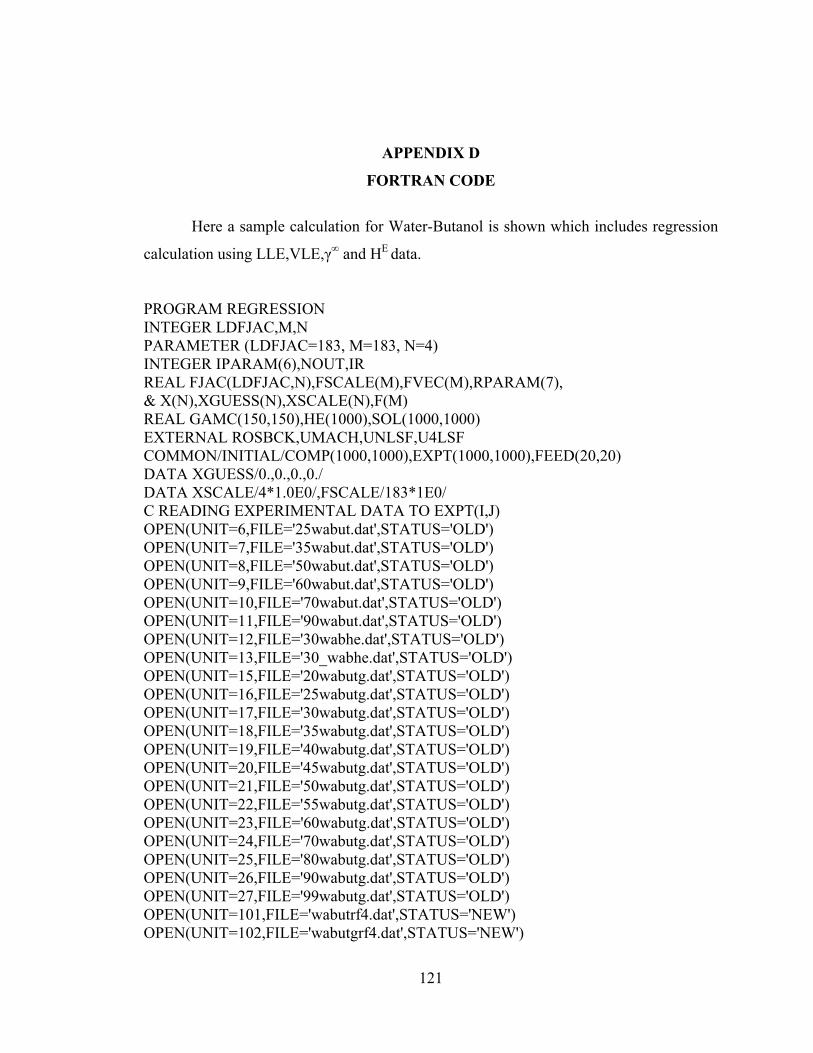
121

APPENDIX D

FORTRAN CODE

Here a sample calculation for Water-Butanol is shown which includes regression

calculation using LLE,VLE,γ∞ and HE data.

PROGRAM REGRESSION INTEGER LDFJAC,M,N PARAMETER (LDFJAC=183, M=183, N=4) INTEGER IPARAM(6),NOUT,IR REAL FJAC(LDFJAC,N),FSCALE(M),FVEC(M),RPARAM(7), & X(N),XGUESS(N),XSCALE(N),F(M) REAL GAMC(150,150),HE(1000),SOL(1000,1000) EXTERNAL ROSBCK,UMACH,UNLSF,U4LSF COMMON/INITIAL/COMP(1000,1000),EXPT(1000,1000),FEED(20,20) DATA XGUESS/0.,0.,0.,0./ DATA XSCALE/4*1.0E0/,FSCALE/183*1E0/ C READING EXPERIMENTAL DATA TO EXPT(I,J) OPEN(UNIT=6,FILE='25wabut.dat',STATUS='OLD') OPEN(UNIT=7,FILE='35wabut.dat',STATUS='OLD') OPEN(UNIT=8,FILE='50wabut.dat',STATUS='OLD') OPEN(UNIT=9,FILE='60wabut.dat',STATUS='OLD') OPEN(UNIT=10,FILE='70wabut.dat',STATUS='OLD') OPEN(UNIT=11,FILE='90wabut.dat',STATUS='OLD') OPEN(UNIT=12,FILE='30wabhe.dat',STATUS='OLD') OPEN(UNIT=13,FILE='30_wabhe.dat',STATUS='OLD') OPEN(UNIT=15,FILE='20wabutg.dat',STATUS='OLD') OPEN(UNIT=16,FILE='25wabutg.dat',STATUS='OLD') OPEN(UNIT=17,FILE='30wabutg.dat',STATUS='OLD') OPEN(UNIT=18,FILE='35wabutg.dat',STATUS='OLD') OPEN(UNIT=19,FILE='40wabutg.dat',STATUS='OLD') OPEN(UNIT=20,FILE='45wabutg.dat',STATUS='OLD') OPEN(UNIT=21,FILE='50wabutg.dat',STATUS='OLD') OPEN(UNIT=22,FILE='55wabutg.dat',STATUS='OLD') OPEN(UNIT=23,FILE='60wabutg.dat',STATUS='OLD') OPEN(UNIT=24,FILE='70wabutg.dat',STATUS='OLD') OPEN(UNIT=25,FILE='80wabutg.dat',STATUS='OLD') OPEN(UNIT=26,FILE='90wabutg.dat',STATUS='OLD') OPEN(UNIT=27,FILE='99wabutg.dat',STATUS='OLD') OPEN(UNIT=101,FILE='wabutrf4.dat',STATUS='NEW') OPEN(UNIT=102,FILE='wabutgrf4.dat',STATUS='NEW')

122

OPEN(UNIT=103,FILE='wabherf4.dat',STATUS='NEW') OPEN(UNIT=104,FILE='solnrf4.dat',STATUS='NEW') DO 103 I=1,6 READ(6,906) (COMP(I,J),J=1,5) 906 FORMAT (5F9.5) 103 CONTINUE DO 104 I=7,13 READ(7,907) (COMP(I,J),J=1,3) 907 FORMAT (3F7.4) 104 CONTINUE DO 105 I=14,42 READ(8,908) (COMP(I,J),J=1,3) 908 FORMAT (3F7.4) 105 CONTINUE DO 106 I=43,47 READ(9,909) (COMP(I,J),J=1,3) 909 FORMAT (3F7.4) 106 CONTINUE DO 107 I=48,53 READ(10,910) (COMP(I,J),J=1,3) 910 FORMAT (3F7.4) 107 CONTINUE DO 108 I=54,59 READ(11,911) (COMP(I,J),J=1,3) 911 FORMAT (3F7.4) 108 CONTINUE DO 109 I=60,68 READ(12,912) (COMP(I,J),J=1,2) 912 FORMAT (2F7.4) 109 CONTINUE DO 110 I=69,80 READ(13,913) (COMP(I,J),J=1,2) 913 FORMAT (2F7.4) 110 CONTINUE FEED(1,1)=.8 FEED(1,2)=.2 c T=15 EXPT(81,1)=.5048 EXPT(81,2)=.0213 c T=20 c EXPT(82,1)=.508 c EXPT(82,2)=.0202 c T=25 EXPT(82,1)=.5056

123

EXPT(82,2)=.0187 c T=30 EXPT(83,1)=.516 EXPT(83,2)=.0182 c T=35 EXPT(84,1)=.523 EXPT(84,2)=.0175 c T=40 EXPT(85,1)=.528 EXPT(85,2)=.0168 c T=50 EXPT(86,1)=.543 EXPT(86,2)=.0165 c T=60 EXPT(87,1)=.5599 EXPT(87,2)=.0162 c T=70 EXPT(88,1)=.58 c EXPT(89,2)=.0167 c T=80 EXPT(89,1)=.597 c EXPT(90,2)=.017 c T=92 EXPT(90,1)=.646 DO 112 I=91,91 READ(15,915) (COMP(I,J),J=1,3) 915 FORMAT (3F7.4) 112 CONTINUE DO 113 I=92,93 READ(16,916) (COMP(I,J),J=1,3) 916 FORMAT (3F7.4) 113 CONTINUE DO 114 I=94,94 READ(17,917) (COMP(I,J),J=1,3) 917 FORMAT (3F7.4) 114 CONTINUE DO 115 I=95,95 READ(18,918) (COMP(I,J),J=1,3) 918 FORMAT (3F7.4) 115 CONTINUE DO 116 I=96,96 READ(19,919) (COMP(I,J),J=1,3) 919 FORMAT (3F7.4) 116 CONTINUE

124

DO 117 I=97,97 READ(20,920) (COMP(I,J),J=1,3) 920 FORMAT (3F7.4) 117 CONTINUE DO 118 I=98,98 READ(21,921) (COMP(I,J),J=1,3) 921 FORMAT (3F7.4) 118 CONTINUE DO 119 I=99,99 READ(22,922) (COMP(I,J),J=1,3) 922 FORMAT (3F7.4) 119 CONTINUE DO 120 I=100,100 READ(23,923) (COMP(I,J),J=1,3) 923 FORMAT (3F7.4) 120 CONTINUE DO 121 I=101,102 READ(24,924) (COMP(I,J),J=1,3) 924 FORMAT (3F7.4) 121 CONTINUE DO 122 I=103,103 READ(25,925) (COMP(I,J),J=1,3) 925 FORMAT (3F7.4) 122 CONTINUE DO 123 I=104,104 READ(26,926) (COMP(I,J),J=1,3) 926 FORMAT (3F7.4) 123 CONTINUE DO 124 I=105,105 READ(27,927) (COMP(I,J),J=1,3) 927 FORMAT (3F7.4) 124 CONTINUE C READING FEED COMPOSITIONS C STARTING REGRESSION CALL U4LSF(IPARAM,RPARAM) RPARAM(4) = 10.0E0*RPARAM(4) CALL UNLSF(ROSBCK,M,N,XGUESS,XSCALE,FSCALE,IPARAM,RPARAM, &X,FVEC,FJAC,LDFJAC) CALL UMACH (2,NOUT) WRITE(*,*) 'SOL',X c WRITE(*,*) 'THE FUNCTION EVALUATED AT THE SOLUTION', FVEC c WRITE(*,*) 'NO. OF ITERATIONS',IPARAM(3) c WRITE(*,*) 'NO. OF FUNCTION EVALUATIONS',IPARAM(4) CALL GAMA(N,X,GAMC)

125

CALL LLEQ(N,X,SOL) CALL EXCS(N,X,HE) err1=0. err2=0. DO 155 I=1,59 IF(I.LT.7)THEN err1=err1+(abs(comp(I,4)-gamc(I,1)))*100./comp(I,4) err2=err2+(abs(comp(I,5)-gamc(I,2)))*100./comp(I,5) WRITE(101,928)comp(I,2),comp(I,4),gamc(I,1),comp(I,5),gamc(I,2), 1 (abs(comp(I,4)-gamc(I,1)))*100./comp(I,4), 2 (abs(comp(I,5)-gamc(I,2)))*100./comp(I,5) ELSE err1=err1+(abs(comp(I,2)-gamc(I,1)))*100./comp(I,2) err2=err2+(abs(comp(I,3)-gamc(I,2)))*100./comp(I,3) WRITE(101,928)comp(I,1),comp(I,2),gamc(I,1),comp(I,3),gamc(I,2), 1 (abs(comp(I,2)-gamc(I,1)))*100./comp(I,2), 2 (abs(comp(I,3)-gamc(I,2)))*100./comp(I,3) ENDIF 928 FORMAT (7F9.5) 155 continue write(101,929) err1/59,err2/59,X 929 FORMAT (9F12.5) err1=0. err2=0. DO 156 I=91,105 err1=err1+(abs(comp(I,2)-gamc(I,1)))*100./comp(I,2) err2=err2+(abs(comp(I,3)-gamc(I,2)))*100./comp(I,3) WRITE(102,930)comp(I,1),comp(I,2),gamc(I,1),comp(I,3),gamc(I,2), 1 (abs(comp(I,2)-gamc(I,1)))*100./comp(I,2), 2 (abs(comp(I,3)-gamc(I,2)))*100./comp(I,3) 930 FORMAT (7F9.5) 156 continue write(102,934) err1/11, err2/11,X 934 FORMAT (9F12.5) err=0. DO 157 I=60,80 err=err+abs((comp(I,2)-HE(I))*100./comp(I,2)) WRITE(103,935)comp(I,1),comp(I,2),HE(I), 1 abs((comp(I,2)-HE(I))*100./comp(I,2)) 935 FORMAT (4F9.3) 157 continue write(103,936) err/21,X 936 FORMAT (8F12.5) er1=0.

126

er2=0. DO 158 I=81,90 IF(I.GT.87) THEN WRITE(104,977)expt(i,1),sol(I,1), 1 abs(expt(i,1)-sol(I,1))*100./expt(i,1) er1=er1+abs(expt(i,1)-sol(I,1))*100./expt(i,1) 977 FORMAT(4F9.5) ELSE WRITE(104,937)expt(i,1),sol(I,1),expt(i,2),sol(I,2), 1 abs(expt(i,1)-sol(I,1))*100./expt(i,1), 2 abs(expt(i,2)-sol(I,2))*100./expt(i,2) er1=er1+abs(expt(i,1)-sol(I,1))*100./expt(i,1) er2=er2+abs(expt(i,2)-sol(I,2))*100./expt(i,2) ENDIF 937 FORMAT(6F9.5) 158 CONTINUE WRITE(104,938)er1/10.,er2/7.,X 938 FORMAT(9F12.5) END SUBROUTINE ROSBCK(M,N,X,F) INTEGER M,N COMMON/INITIAL/COMP(1000,1000),EXPT(1000,1000),FEED(20,20) REAL X(N),F(M),REG(7),FIR(6),GAMC(150,150),HE(1000), 1 SOL(1000,1000) CALL GAMA(N,X,GAMC) CALL LLEQ(N,X,SOL) CALL EXCS(N,X,HE) IR=1 DO 9 I=1,6 F(IR)=(COMP(I,4) - GAMC(I,1)) / COMP(I,4) F(IR)=F(IR)*1. IR=IR+1 F(IR)=(COMP(I,5) - GAMC(I,2)) / COMP(I,5) F(IR)=F(IR)*1. IR=IR+1 9 CONTINUE DO 10 I=7,59 F(IR) = (COMP(I,2) - GAMC(I,1)) / COMP(I,2) IR=IR+1 F(IR) = (COMP(I,3) - GAMC(I,2)) / COMP(I,3) IR=IR+1 10 CONTINUE DO 11 I=60,80 F(IR)=(COMP(I,2) - HE(I)) / COMP(I,2)

127

F(IR)=F(IR)*1. IR=IR+1 11 CONTINUE DO 12 I = 81,90 DO 14 J=1,2 F(IR) = (EXPT(I,J) - SOL(I,J)) / EXPT(I,J) IF(I.EQ.81.AND.J.EQ.2) F(IR)=F(IR)*4.5 IF(I.GT.87)GOTO 12 IR=IR+1 14 CONTINUE 12 CONTINUE DO 13 I=91,105 F(IR) = (COMP(I,2) - GAMC(I,1)) / COMP(I,2) F(IR)=F(IR)*1. IF(I.EQ.92)F(IR)=F(IR)*1. IR=IR+1 F(IR) = (COMP(I,3) - GAMC(I,2)) / COMP(I,3) F(IR)=F(IR)*1. IF(I.EQ.93)F(IR)=F(IR)*1. IR=IR+1 13 CONTINUE RETURN END SUBROUTINE GAMA(N,X,GAMC) COMMON/BINARY/A(100,100),B(100,100),C(100,100),AL(100,100) COMMON/INITIAL/COMP(1000,1000),EXPT(1000,1000),FEED(20,20) REAL Z(20),GAM(20),tau(20,20) INTEGER NC,ID(20),ERR,N DIMENSION GAMC(150,150),X(N) NC = 2 A(1,1)=0. A(1,2)= 1031.46 A(2,1)= 229.43 A(2,2)=0. B(1,1)=0. B(1,2)=X(1) B(2,1)=X(3) B(2,2)=0. C(1,1)=0. C(1,2)=X(2) C(2,1)=X(4) C(2,2)=0. AL(1,2)=.4081 AL(2,1)=AL(1,2)

128

ID(1)=1 ID(2)=2 KEY=1 C COMP(1,1)=0. C COMP(2,1)=1. C N,ID,KEY,X,T,GAM,ERG DO 103 I=1,6 Z(1)=COMP(I,2) Z(2)=1.-Z(1) T = 273.15+25 CALL nrtl(NC,ID,KEY,Z,T,GAM,ERR) GAMC(I,1) = GAM(1) GAMC(I,2) = GAM(2) 103 CONTINUE DO 104 I=7,13 Z(1)=COMP(I,1) Z(2)=1.-Z(1) T = 273.15+35 CALL nrtl(NC,ID,KEY,Z,T,GAM,ERR) GAMC(I,1) = GAM(1) GAMC(I,2) = GAM(2) c print*,GAMC(I,1),GAMC(I,2) 104 CONTINUE DO 105 I=14,42 Z(1)=COMP(I,1) Z(2)=1.-Z(1) T = 273.15+50 CALL nrtl(NC,ID,KEY,Z,T,GAM,ERR) GAMC(I,1) = GAM(1) GAMC(I,2) = GAM(2) C print*, GAMC(I,1),GAMC(I,2) 105 CONTINUE DO 106 I=43,47 Z(1)=COMP(I,1) Z(2)=1.-Z(1) T = 273.15+60 CALL nrtl(NC,ID,KEY,Z,T,GAM,ERR) GAMC(I,1) = GAM(1) GAMC(I,2) = GAM(2) C print*, GAMC(I,1),GAMC(I,2) 106 CONTINUE DO 107 I=48,53 Z(1)=COMP(I,1) Z(2)=1.-Z(1)

129

T = 273.15+70 CALL nrtl(NC,ID,KEY,Z,T,GAM,ERR) GAMC(I,1) = GAM(1) GAMC(I,2) = GAM(2) C print*, GAMC(I,1),GAMC(I,2) 107 CONTINUE DO 108 I=54,59 Z(1)=COMP(I,1) Z(2)=1.-Z(1) T = 273.15+90 CALL nrtl(NC,ID,KEY,Z,T,GAM,ERR) GAMC(I,1) = GAM(1) GAMC(I,2) = GAM(2) C print*, GAMC(I,1),GAMC(I,2) 108 CONTINUE DO 112 I=91,91 Z(1)=COMP(I,1) Z(2)=1.-Z(1) T = 273.15+20 CALL nrtl(NC,ID,KEY,Z,T,GAM,ERR) GAMC(I,1) = GAM(1) GAMC(I,2) = GAM(2) C print*, GAMC(I,1),GAMC(I,2) 112 CONTINUE DO 113 I=92,93 Z(1)=COMP(I,1) Z(2)=1.-Z(1) T = 273.15+25 CALL nrtl(NC,ID,KEY,Z,T,GAM,ERR) GAMC(I,1) = GAM(1) GAMC(I,2) = GAM(2) C print*, GAMC(I,1),GAMC(I,2) 113 CONTINUE DO 114 I=94,94 Z(1)=COMP(I,1) Z(2)=1.-Z(1) T = 273.15+30 CALL nrtl(NC,ID,KEY,Z,T,GAM,ERR) GAMC(I,1) = GAM(1) GAMC(I,2) = GAM(2) C print*, GAMC(I,1),GAMC(I,2) 114 CONTINUE DO 115 I=95,95 Z(1)=COMP(I,1)

130

Z(2)=1.-Z(1) T = 273.15+35 CALL nrtl(NC,ID,KEY,Z,T,GAM,ERR) GAMC(I,1) = GAM(1) GAMC(I,2) = GAM(2) C print*, GAMC(I,1),GAMC(I,2) 115 CONTINUE DO 116 I=96,96 Z(1)=COMP(I,1) Z(2)=1.-Z(1) T = 273.15+40 CALL nrtl(NC,ID,KEY,Z,T,GAM,ERR) GAMC(I,1) = GAM(1) GAMC(I,2) = GAM(2) C print*, GAMC(I,1),GAMC(I,2) 116 CONTINUE DO 117 I=97,97 Z(1)=COMP(I,1) Z(2)=1.-Z(1) T = 273.15+45 CALL nrtl(NC,ID,KEY,Z,T,GAM,ERR) GAMC(I,1) = GAM(1) GAMC(I,2) = GAM(2) C print*, GAMC(I,1),GAMC(I,2) 117 CONTINUE DO 118 I=98,98 Z(1)=COMP(I,1) Z(2)=1.-Z(1) T = 273.15+50 CALL nrtl(NC,ID,KEY,Z,T,GAM,ERR) GAMC(I,1) = GAM(1) GAMC(I,2) = GAM(2) C print*, GAMC(I,1),GAMC(I,2) 118 CONTINUE DO 119 I=99,99 Z(1)=COMP(I,1) Z(2)=1.-Z(1) T = 273.15+55 CALL nrtl(NC,ID,KEY,Z,T,GAM,ERR) GAMC(I,1) = GAM(1) GAMC(I,2) = GAM(2) C print*, GAMC(I,1),GAMC(I,2) 119 CONTINUE DO 120 I=100,100

131

Z(1)=COMP(I,1) Z(2)=1.-Z(1) T = 273.15+60 CALL nrtl(NC,ID,KEY,Z,T,GAM,ERR) GAMC(I,1) = GAM(1) GAMC(I,2) = GAM(2) C print*, GAMC(I,1),GAMC(I,2) 120 CONTINUE DO 121 I=101,102 Z(1)=COMP(I,1) Z(2)=1.-Z(1) T = 273.15+70 CALL nrtl(NC,ID,KEY,Z,T,GAM,ERR) GAMC(I,1) = GAM(1) GAMC(I,2) = GAM(2) C print*, GAMC(I,1),GAMC(I,2) 121 CONTINUE DO 122 I=103,103 Z(1)=COMP(I,1) Z(2)=1.-Z(1) T = 273.15+80 CALL nrtl(NC,ID,KEY,Z,T,GAM,ERR) GAMC(I,1) = GAM(1) GAMC(I,2) = GAM(2) C print*, GAMC(I,1),GAMC(I,2) 122 CONTINUE DO 123 I=104,104 Z(1)=COMP(I,1) Z(2)=1.-Z(1) T = 273.15+90 CALL nrtl(NC,ID,KEY,Z,T,GAM,ERR) GAMC(I,1) = GAM(1) GAMC(I,2) = GAM(2) C print*, GAMC(I,1),GAMC(I,2) 123 CONTINUE DO 124 I=105,105 Z(1)=COMP(I,1) Z(2)=1.-Z(1) T = 273.15+99 CALL nrtl(NC,ID,KEY,Z,T,GAM,ERR) GAMC(I,1) = GAM(1) GAMC(I,2) = GAM(2) C print*, GAMC(I,1),GAMC(I,2) 124 CONTINUE

132

RETURN END SUBROUTINE EXCS(N,X,HE) COMMON/BINARY/A(100,100),B(100,100),C(100,100),AL(100,100) COMMON/INITIAL/COMP(1000,1000),EXPT(1000,1000),FEED(20,20) REAL HE(1000),HEE,Z(20) INTEGER N DIMENSION X(N) A(1,1)=0. A(1,2)= 1031.46 A(2,1)= 229.43 A(2,2)=0. B(1,1)=0. B(1,2)=X(1) B(2,1)=X(3) B(2,2)=0. C(1,1)=0. C(1,2)=X(2) C(2,1)=X(4) C(2,2)=0. AL(1,2)=.4081 AL(2,1)=AL(1,2) DO 109 I=60,68 Z(1)=COMP(I,1) Z(2)=1.-Z(1) T = 273.15+30 CALL ENTH(Z,T,HEE) HE(I)=HEE C print*, HE 109 CONTINUE DO 110 I=69,80 Z(1)=COMP(I,1) Z(2)=1.-Z(1) T=273.15+30 CALL ENTH(Z,T,HEE) HE(I)=HEE C print*, HE 110 CONTINUE RETURN END SUBROUTINE LLEQ(N,X,SOL) COMMON/BINARY/A(100,100),B(100,100),C(100,100),AL(100,100) COMMON/INITIAL/COMP(1000,1000),EXPT(1000,1000),FEED(20,20) REAL K(20),Z(20),GAE(20),GAR(20)

133

INTEGER ID(20),ERR,NC,N DIMENSION XE(20), XR(20),SOL(1000,1000),X(N) REAL GAME(20), GAMR(20) NC = 2 ID(1) = 1 ID(2) = 2 A(1,1)=0. A(1,2)= 1031.46 A(2,1)= 229.43 A(2,2)=0. B(1,1)=0. B(1,2)=X(1) B(2,1)=X(3) B(2,2)=0. C(1,1)=0. C(1,2)=X(2) C(2,1)=X(4) C(2,2)=0. AL(1,2)=.4081 AL(2,1)=AL(1,2) Z(1) = FEED(1,1) Z(2) = FEED(1,2) KEY = 1 IR=1 IE=2 T=273.15+15 CALL ELIPS(NC,ID,KEY,IR,IE,Z,T,A,XR,XE,K,ERR) SOL(81,1) = XE(1) SOL(81,2) = XR(2) c print*,sol(91,1),sol(91,2) c T=273.15+20 c CALL ELIPS(NC,ID,KEY,IR,IE,Z,T,A,XR,XE,K,ERR) c SOL(82,1) = XE(1) c SOL(82,2) = XR(2) T=273.15+25 CALL ELIPS(NC,ID,KEY,IR,IE,Z,T,A,XR,XE,K,ERR) SOL(82,1) = XE(1) SOL(82,2) = XR(2) T=273.15+30 CALL ELIPS(NC,ID,KEY,IR,IE,Z,T,A,XR,XE,K,ERR) SOL(83,1) = XE(1) SOL(83,2) = XR(2) T=273.15+35 CALL ELIPS(NC,ID,KEY,IR,IE,Z,T,A,XR,XE,K,ERR)

134

SOL(84,1) = XE(1) SOL(84,2) = XR(2) T=273.15+40 CALL ELIPS(NC,ID,KEY,IR,IE,Z,T,A,XR,XE,K,ERR) SOL(85,1) = XE(1) SOL(85,2) = XR(2) T=273.15+50 CALL ELIPS(NC,ID,KEY,IR,IE,Z,T,A,XR,XE,K,ERR) SOL(86,1) = XE(1) SOL(86,2) = XR(2) T=273.15+60 CALL ELIPS(NC,ID,KEY,IR,IE,Z,T,A,XR,XE,K,ERR) SOL(87,1) = XE(1) SOL(87,2) = XR(2) T=273.15+70 CALL ELIPS(NC,ID,KEY,IR,IE,Z,T,A,XR,XE,K,ERR) SOL(88,1) = XE(1) SOL(88,2) = XR(2) T=273.15+80 CALL ELIPS(NC,ID,KEY,IR,IE,Z,T,A,XR,XE,K,ERR) SOL(89,1) = XE(1) SOL(89,2) = XR(2) T=273.15+92 CALL ELIPS(NC,ID,KEY,IR,IE,Z,T,A,XR,XE,K,ERR) SOL(90,1) = XE(1) SOL(90,2) = XR(2) C print*,sol(1,1),sol(1,2) RETURN END SUBROUTINE ELIPS(N,ID,KEY,IR,IE,Z,T,A,XR,XE,K,ERR) C ELIPS CALCULATES CONJUGATE PHASE COMPOSITIONS XR AND XE FOR C PARTIALLY MISCIBLE N COMPONENT LIQUID SYSTEMS OF OVERALL COMPOSTION C Z AT GIVEN TEMPERATURE T(K). INDICES OF THE COMPONENTS INVOLVED C SHOULD BE IN THE VECTOR ID. IR AND IE ARE THE COMPONENT NRS OF THE C R AND E PHASE SOLVENTS (SHOULD BE ..................) REAL Z(N),XR(N),XE(N),K(N),GAR(20),GAE(20),K1(20),KS,KP,K2, 1 RX(20),EX(20) INTEGER ID(N),ERR,ERL 100 ERR = 0 KEE = KEY IF (IR.EQ.0.OR.IE.EQ.0) GO TO 101

135

GO TO(101,130,130,130,130,130,130,130,101,130),KEY C FOR NEW SYSTEMS WITHOUT IR, IE SPECIFIED, FIND IR, IE AS LEAST SOLUBLE C PAIR 101 KS = 1. KP = 1. 110 DO 115 I=1,N XR(I) = 0. 115 XE(I) = 0. J1 = 1 IF (IR.NE.0) GO TO 120 IF (IE.NE.0) GO TO 121 116 DO 119 J=2,N XR(J1) = 0. XE(J1) = 0. J1 = J-1 XR(J) = 0.98 XE(J) = 0.02 XR(J-1) = 0. XE(J-1) = 0. IF(Z(J).LT.0.10) GO TO 119 DO 118 I=1,J1 XE(I) = 0.98 XR(I) = 0.02 IF(I.GT.1) XE(I-1) = 0. IF(I.GT.1) XR(I-1) = 0. IF(Z(I).LT.0.10) GO TO 118 CALL LILIK(N,ID,KEE,XR,XE,T,K,GAR,GAE,ERL) IF(ERL.GT.1) GO TO 900 KEE = 3 IF(K(I).LE.KS) GO TO 117 KS = K(I) IS = I 117 IF(1./K(J).LE.KS) GO TO 118 KS = 1./K(J) IS = J 118 CONTINUE 119 CONTINUE XR(N) = 0. XE(N) = 0. XR(J1) = 0. XE(J1) = 0. GO TO 125 120 IF(IE.NE.0) GO TO 130

136

IS = IR GO TO 125 121 IS = IE 125 XE(IS) = 0.98 XR(IS) = 0.02 126 DO 129 J=1,N IF(J.EQ.IS) GO TO 129 XR(J) = 0.98 XE(J) = 0.02 IF(J.EQ.(IS+1)) GO TO 128 IF(J.GT.1) XR(J-1) = 0. IF(J.GT.1) XE(J-1) = 0. 127 IF(Z(J).LT.0.10) GO TO 129 CALL LILIK(N,ID,KEE,XR,XE,T,K,GAR,GAE,ERL) IF(ERL.GT.1) GO TO 900 KEE = 3 IF(K(J).GE.KP) GO TO 129 KP = K(J) IP = J GO TO 129 128 IF(J.GT.2) XR(J-2) = 0. IF(J.GT.2) XE(J-2) = 0. GO TO 127 129 CONTINUE IE = IP IF(IR.NE.IS) IE = IS IF(IR.NE.IS) IR = IP C INITIALIZE R AND E PHASE COMPOSITIONS 130 DO 131 I=1,N XR(I) = 0. 131 XE(I) = 0. XR(IR) = 0.98 XE(IR) = 0.02 XR(IE) = 0.02 XE(IE) = 0.98 C GET INITIAL ESTIMATES FOR K VALUES 135 CALL LILIK(N,ID,KEE,XR,XE,T,K,GAR,GAE,ERL) IF(ERL.GT.1) GO TO 900 SZ = 0. 136 DO 137 I=1,N SZ = SZ+Z(I) 137 K1(I) = K(I)-1 IF(ABS(SZ-1.).GT.0.01) GO TO 903 C GET INITIAL ESTIMATE FOR A

137

A = Z(IE)/(Z(IE)+Z(IR)) A = -A/K1(IR)+(A-1.)/K1(IE) IF(A.LT.0.) A=0. IF(A.GT.1.) A=1. A0 = A IT = 0 KAC = 0 C CONDUCT ITERATION OVER PHASE COMPOSTION (OUTER LOOP) 200 IT = IT+1 IF(IT.GT.50) GO TO 900 AA = A0 A0 = A AN = A C CONDUCT NEWTON-RAPHSON ITERATION FOR A AT FIXED K VALUES 300 DO 319 M=1,10 F = 0. DF = 0. 301 DO 309 I = 1,N K2 = A*K1(I)+1. F = F+Z(I)*K1(I)/K2 309 DF = DF-Z(I)*(K1(I)/K2)**2 IF(ABS(F).LT.1.E-05) GO TO 210 DA = F/DF 310 AN = A-DA C LIMIT A TO RANGE 0-1 IF IT FALLS OUTSIDE POLES OF F IF(AN.LT.-1./K1(IR)) GO TO 312 AN = A+(1./K1(IR)+A)/2. GO TO 319 312 IF(AN.GT.-1./K1(IE)) GO TO 319 AN=A+(1./K1(IE)+A)/2. 319 A = AN GO TO 900 210 A = AN SR = 0. SE = 0. C FIND NEW R AND E PHASE COMPOSITIONS 211 DO 215 I=1,N XR(I) = Z(I)/(A*K1(I)+1.) XE(I) = K(I)*XR(I) SR = SR+XR(I) 215 SE = SE+XE(I) 220 DO 225 I=1,N XR(I) = XR(I)/SR 225 XE(I) = XE(I)/SE

138

C AT ALTERNATE ITERATIONS AFTER 3 ACCELERATE PHASE COMPOSITIONS BY C WEGSTEIN METHOD BASED ON SUM OF DEVIATIONS OF COMPONENT FUGACITITES 230 IF(IT.LT.3) GO TO 250 IF(IT.LE.5.AND.(A.LT.0..OR.A.GT.1.)) GO TO 250 IF(KAC.GE.1) GO TO 239 IF(SS.GT.SL) GO TO 250 IF(SS.GT.0.2) GO TO 250 KAC = 1 WG = SS/(SL-SS) WK = 1.+WG SR = 0. SE = 0. DO 235 I=1,N XR(I) = WK*XR(I)-WG*RX(I) C ALLOW NO NEGATIVE MOL FRACTIONS IF(XR(I).LT.0.) XR(I) = 0. XE(I) = WK*XE(I)-WG*EX(I) IF(XE(I).LT.0.) XE(I) = 0. SR = SR+XR(I) 235 SE = SE+XE(I) C NORMALIZE ACCELERATED COMPOSITIONS (TO ALLOW FOR XR(I) OR XE(I) SET C TO 0) 236 DO 237 I=1,N XR(I) = XR(I)/SR 237 XE(I) = XE(I)/SE GO TO 250 239 KAC = 0 C NEW K AND GAMMA VALUES 250 CALL LILIK(N,ID,3,XR,XE,T,K,GAR,GAE,ERL) IF(ERL.GT.1) GO TO 900 ESS = 1.E-03 IF(IT.LE.5) GO TO 252 C CHECK FOR VICINITY OF A PLAIT POINT PPI = K(IR)/K(IE)+K(IE)/K(IR) IF(PPI.GT.10..OR.SS.GT.0.05) GO TO 251 C EXIT IF TOO NEAR PLAIT POINT IF(IT.GE.20) GO TO 290 IF(PPI.GT.7.) GO TO 251 C CHECK IF CALCULATION NEAR PLAIT POINT IS PROBABLY IN SINGLE PHASE C REGION--IF SO CONTINUE

139

DE=A0 IF(DE.GT.0.5) DE=A0-1. DI = (AA-A)/DE IF(DI.LT.0.1) GO TO 290 251 IF(PPI.LT.20) ESS = 2.E-04 252 SL = SS SS = 0. 253 DO 255 I=1,N K1(I) = K(I)-1. C CALCULATE OBJECTIVE FUNCTION 255 SS = SS+ABS(GAE(I)*XE(I)-GAR(I)*XR(I)) C CHECK CONVERGENCE IF(SS.LE.ESS) GO TO 190 IF(A.GE.0..AND.A.LE.1.) GO TO 260 IF(IT.LT.3.OR.SS.GT.0.20) GO TO 260 IF(IT.LT.5.AND.SS.GT.0.05) GO TO 260 C CHECK IF A MOVING AWAY FROM 0 - 1 REGION WRITE(*,*) 'DONE',A,A0 IF((ABS(A)-ABS(A0)).GT.0.) GO TO 195 C SAVE LAST PHASE COMPOSITIONS FOR USE IN ACCELERATION 260 DO 265 I=1,N RX(I) = XR(I) 265 EX(I) = XE(I) GO TO 200 C FEED IN VICINITY OF PLAIT POINT -- CHECK IF IN TWO PHASE REGION 290 IF(A.GE.0..AND.A.LE.1.) GO TO 905 GO TO 195 C DO NOT ALLOW CONVERGENCE ON ACCELERATED ITERATION 190 IF(KAC.EQ.1) GO TO 260 C CONVERGED SOLUTION--CHECK IF IN TWO PHASE REGION 191 IF(A.LT.0..OR.A.GT.1.) GO TO 195 ERR = ERL RETURN C FEED OUTSIDE TWO PHASE REGION 195 DO 196 I=1,N WRITE(*,*) 'JUNK' XR(I) = Z(I) 196 XE(I) = Z(I) IF(A.LT.0.) A=0. IF(A.GT.1.) A=1. ERR=ERL RETURN C ON FAILURE TO CONVERGE SET A TO -1 AND ERR TO 2 900 ERR = 2

140

GO TO 910 C FOR BAD INPUT DATA SET A TO -1 AND ERR TO 5 903 ERR = 5 GO TO 910 C FOR FEED TOO NEAR PLAIT POINT SET A TO -1 AND ERR TO 7 905 ERR = 7 910 DO 911 I=1,N XR(I) = Z(I) 911 XE(I) = Z(I) A = -1 RETURN END SUBROUTINE LILIK(N,ID,KEY,XR,XE,T,K,GAR,GAE,ERR) REAL XR(N),XE(N),K(N),GAR(N),GAE(N),X(20),Y(20),GX(20),GY (20) INTEGER ID(N),IDF(20),ERR,ERG 100 ERR = 0 C CONVERT COMPOSITION VECTORS TO DIMENSION 20 TO MATCH LOWER LEVEL C SUBROUTINES 101 DO 102 I=1,N X(I) = XR(I) Y(I) = XE(I) 102 IDF(I) = ID(I) C GET R AND E PHASE ACTIVITY COEFFICIENT VECTORS TO DIMENSION N CALL NRTL(N,IDF,KEY,X,T,GX,ERG) CALL NRTL(N,IDF,3,Y,T,GY,ERG) C CONVERT ACTIVITY COEFFICIENT VECTORS TO DIMENSION N 110 DO 119 I=1,N GAR(I) = GX(I) GAE(I) = GY(I) K(I) = GAR(I)/GAE(I) IF(K(I).LE.0..OR.K(I).GT.1.E+19) GO TO 900 119 CONTINUE ERR = ERG RETURN C FOR A K VALUE OUT OF RANGE SET ERR TO 2 900 ERR = 2 DO 905 I=1,N 905 K(I)=0. RETURN END SUBROUTINE NRTL(N,ID,KEY,X,T,GAM,ERG) C STGX=SUMMATION OF PRODUCT TAU,G,X C SGX=SUMMATION OF PRODUCT G,X

141

C XG=PRODUCT OF X,G C SGX=SUMMATION OF PRODUCT G,X C SXTG=SUMMATION OF PRODUCT X,TAU,G C TAU=TAU(I,J) C SG FOR 'g',AL FOR ALPHA REAL X(20),GAM(20),STGX,SGX1,SGX2,SGX3,SXTG,ST2, 1 TAU(20,20),G(20,20),SG(20,20) COMMON/BINARY/A(100,100),B(100,100),C(100,100),AL(100,100) integer bb,cc,r do 15 bb=1,n do 25 cc=1,n sg(bb,cc)=A(bb,cc)+B(bb,cc)*(T-298.15)+C(bb,cc)*(T-298.15)**2 tau(bb,cc)=sg(bb,cc)/T G(bb,cc)=exp(-AL(bb,cc)*tau(bb,cc)) 25 continue 15 continue DO 120 I=1,N SGX1=0. ST2=0. STGX=0. DO 121 J=1,N STGX=STGX+TAU(J,I)*G(J,I)*X(J) 121 CONTINUE DO 122 L=1,N SGX1=SGX1+G(L,I)*X(L) 122 CONTINUE DO 123 J=1,N sgx2=0. sxtg=0. sgx3=0. DO 124 L=1,N SGX2=SGX2+G(L,J)*X(L) 124 CONTINUE DO 125 R=1,N SXTG=SXTG+X(R)*TAU(R,J)*G(R,J) 125 CONTINUE DO 126 L=1,N SGX3=SGX3+G(L,J)*X(L) 126 CONTINUE ST2=ST2+X(J)*G(I,J)/SGX2*(TAU(I,J)-SXTG/SGX3) 123 CONTINUE GAM(I)=EXP(STGX/SGX1+ST2) 120 CONTINUE RETURN

142

END SUBROUTINE ENTH(X,T,HE) C TAU=TAU(I,J) C SG FOR 'g',AL FOR ALPHA REAL X(20),TAU(20,20),G(20,20),SG(20,20),HE,T COMMON/BINARY/A(100,100),B(100,100),C(100,100),AL(100,100) integer bb,cc do 15 bb=1,2 do 25 cc=1,2 sg(bb,cc)=A(bb,cc)+B(bb,cc)*(T-298.15)+C(bb,cc)*(T-298.15)**2 tau(bb,cc)=sg(bb,cc)/T G(bb,cc)=exp(-AL(bb,cc)*tau(bb,cc)) 25 continue 15 continue A12=A(1,2) A21=A(2,1) B12=B(1,2) B21=B(2,1) C12=C(1,2) C21=C(2,1) G12=G(1,2) G21=G(2,1) sg12=sg(1,2) sg21=sg(2,1) TAU12=TAU(1,2) TAU21=TAU(2,1) ALP=AL(1,2) x1=X(1) x2=1.-x1 c HE=x1*x2*(G21*(A21-2*C21*T**2)/(x1+x2*G21)**2*(x1*(1.-ALP* c 1 TAU21)+x2*G21)+G12*(A12-2*C12*T**2)/(x2+x1*G12)**2*(x2*(1.-ALP* c 2 TAU12)+x1*G12)) HE=(x1*x2*G21/(x1+x2*G21))*(-1.+ALP*x1*TAU21/(x1+x2*G21))* 1 (B21*T+2*C21*T*(T-298.15)-sg21)+ 2 (x1*x2*G12/(x2+x1*G12))*(-1.+ALP*x2*TAU12/(x2+x1*G12))* 3 (B12*T+2*C12*T*(T-298.15)-sg12) HE=HE*8.314 RETURN END

143

APPENDIX E

TERNARY DATA

Table E1. Experimental Ternary Data for Hexane – 1-Butanol – Water (in mole percent) [1] Hexane – Rich Phase Water – Rich Phase

Hexane 1-Butanol Water Hexane 1-Butanol Water 99.791 0.209 0.000 0 0.170 99.830 99.544 0.456 0.000 0 0.343 99.657 99.057 0.943 0.000 0 0.550 99.450 98.444 1.556 0.000 0 0.695 99.305 97.826 2.174 0.000 0 0.792 99.208 97.225 2.775 0.000 0 0.819 99.181 96.756 3.244 0.000 0 0.885 99.115 96.607 3.393 0.000 0 0.887 99.113 95.694 4.306 0.000 0 0.955 99.045 96.964 3.036 0.000 0 0.871 99.129 95.280 4.720 0.000 0 0.997 99.003 93.336 6.664 0.000 0 1.077 98.923 93.030 6.410 0.560 0 1.037 98.963 88.656 10.301 1.043 0 1.144 98.856 83.966 14.224 1.810 0 1.216 98.784 80.071 17.338 2.591 0 1.228 98.772 75.459 21.029 3.512 0 1.279 98.721 71.569 23.895 4.536 0 1.326 98.674 65.068 28.635 16.296 0 1.348 98.652 24.740 52.850 22.410 0 1.411 98.589 16.978 55.206 27.816 0 1.451 98.449 11.762 56.548 31.690 0 1.480 98.520

144

Table E2. Experimental Ternary Data for Hexane – 1-Butanol – Water (in mole percent) [22]

Hexane – Rich Phase Water – Rich Phase Hexane 1-Butanol Water Hexane 1-Butanol Water 83.28 15.40 01.32 0 00.66 99.34 76.01 21.18 02.81 0 00.71 99.29 55.71 35.47 08.82 0 00.80 99.20 44.60 42.07 13.33 0 00.90 99.10 29.83 49.42 20.75 0 01.02 98.98 19.89 53.11 27.00 0 01.20 98.80 06.69 54.13 39.18 0 01.29 98.71

145

APPENDIX F

TABLES OF DATA SELECTION OVER THE TEMPERATURE RANGE 10-100 °C

Table F1. Binary data selection over the temperature range 10-100 °C

Binary pair Type of data Temp(°C) Data[Ref]

Hexane-Water Butanol-Water

Solubility of Hexane in Water Solubility of Water in Hexane Solubility of Butanol in Water Solubility of Water in Butanol γ∞ of Butanol γ∞ of Water

25 35 93 100 25 40 93 100 15 25 30 35 40 50 60 70 80 92 15 25 30 35 40 50 60 20 25 30 35 40 45 50 55 60 70 25 70

2.57E-06 [from @25°C selection] 2.69E-06 [20] 5.73E-06 [20] 6.21E-06 [20] 4.7E-04 [from @25°C selection] 1.5E-03 [20] 5.95E-03 [20] 7.09E-03 [20] .5048 [36] .506 [from @25 °C selection] .511 [36] .516 [36] .523 [36] .528 [36] .543 [36] .559 [36] .581 [36] .597 [36] .021 [36] .0187 [from @25 °C selection] .0181 [36] .0175 [36] .0168 [36] .0165 [36] .0162 [73] 48.4 [35] 51.37 [from @25 °C selection] 53.4 [35] 57.2 [35] 58.9 [35] 60.2 [35] 61.5 [35] 62.8 [35] 63.4 [35] 63.8 [35] 5.06 [from @25 °C selection] 3.27 [80]

146

Hexane-Butanol

VLE HE γ∞ of Hexane γ∞ of Butanol VLE HE

80 90 99 25 35 50 60 70 90 30 30 30 25 50 60 25 42 58 67 25 30 35 40 45 50 59 65 75 15 25 35 45

3.12 [80] 3.07 [80] 2.97 [80] [from @25 C selection] [71] [78] [43] [72] [72] [74] [74] [83] 5.12 [from @25 °C selection] 5.6 [65] 5.3 [65] 38.6 [from @25 °C selection] 22.5 [41] 15.1 [41] 12.2 [41] [from @25 °C selection] [48] [48] [48] [48] [48] [76] [76] [76] [89] [from @25 °C selection] [82] [82]