-tiLt LuriPoverty and Growth in Kenya

INTEANATIONL MONETARy FUND

SWP389

World Bank Staff Working Paper No. 389

May 1980

Prepared by: Paul Collier (Consultant)Deepak Lal, Development Economics Department

Copyright © 1980The World Bank1818 H Street, N.W.Washington, D.C. 20433, U.S.A.

The views and interpretations in this document are those of theauthors and should not be attributed to the World Bank, to itsIIraffiliated organizations, or to any individual acting in their behalf. FIL 1 COpy

Pub

lic D

iscl

osur

e A

utho

rized

Pub

lic D

iscl

osur

e A

utho

rized

Pub

lic D

iscl

osur

e A

utho

rized

Pub

lic D

iscl

osur

e A

utho

rized

Pub

lic D

iscl

osur

e A

utho

rized

Pub

lic D

iscl

osur

e A

utho

rized

Pub

lic D

iscl

osur

e A

utho

rized

Pub

lic D

iscl

osur

e A

utho

rized

The views and interpretations in this document are those of the authorand should not be attributed to the World Bank, to its affiliatedorganizations, or to any individual acting in their behalf.

WORLD BANK

Staff Working Paper No. 389

May 1980

POVERTY AND GROWTH IN KENYA

Chapters 1 and 2 of this paper provide an empirical investigation oftrends in poverty and income distribution in Kenya between 1963 and 1974,differentiated by region and occupation. Chapter 3 provides a framework forexplaining these trends in terms of the pattern of growth, and in particularemphasizes the two way rural-urban interactions which largely explain the"spread" effects of growth in Kenya. Chapter 4 derives some policy conclusionson how future growth could be made to yield even higher degrees of povertyredressal.

- The research was begun when both researchers worked as consultantsto the Eastern African Regional Office of the Bank, and was completedafter the second author joined the Development Economics Department. Partof the research has been funded through RPO 671-84.

Prepared by: Paul Collier (Consultant)Deepak Lal, Development Economics Department

Copyright 01980The World Bank1818 H Street, N.W.Washington, D.C. 20433, U.S.A.

POVERTY AND GROWTH IN KENYA

By

Paul Collier and Deepak Lal

Contents

PaRe No.

Chapter 1 Overall Trends in Poverty, IncomeDistribution, and Growth ..................... 1

Chapter 2 The Characteristics of the Poor ............... 12

Chapter 3 Poverty and Growth: Rural-Urban Interactions . 35

Chapter 4 Policy Implications ..... *... ... *................ 59

Appendix 1 Poverty Lines ...... . .... . .. . * .. ........................ . 68

Appendix 2 The Innovation Index ......................... 69

List of Tables in the Main Report

Page No.

Table 1 Poverty in Kenya - 1974 ................ * .......... 2

Table 2 Trends in Absolute Poverty 1963-74 ................ 4

Table 3 The Distribution of Income in Kenya, 1974 ......... 4

Table 4 The Distribution of Income in Kenya by EconomicStatus of Household ............................. 5

Table 5 Trends in Income Distribution, 1963-74 .............. 7

Table 6 Trends in the Distribution of SmallholderConsumption, 1963-74 .......................... . 9

Table 7 Landholding of those Cultivating Land onSmallholdings ............................. . ................... 10

Table 8 Characteristics of the Smallholder Poor ........... 12

Table 9 Smallholder Poverty by Region, 1974 ........ .......... 13

Table 10 Smallholder Characteristics by Income and Province

Table 11 Direct Inputs Associated with an Increase inFarm Inocme of 1,000s.p.a. for Three Regions .... 14

Table 12 Mean Smallholder Incomes and Use of DirectInputs for Three Provinces ...................... 16

Table 13 Direct and Indirect Farm Inputs for ThreeProvinces ....... .................. ............................ 18

Table 14 Farmers' Ranking of Different Sources of Income ... 20

Table 15 Why Poor Smallholders have low Non-Farm Incomes,for Three Provinces ............... ..... ...... 22

Table 16 Sources of Mean Smallholder Non-Farm Income forThree Provinces .................................. 23

Table 17 Urban-Based Non-Farm Income and Ecucation ......... 23

Table 18 Innovation and Education ........ ....... . . ..... 24

Table 19 The Rural Landless by Occupation, 1976 ....... ...... 25

Table 20 The Landless in Low Income Activities by Province . 26

Table 2.1 Income, Food Consumption and Nutrition ofLaborers and Smallholders ....... ............ 27

Page No.

Table 22 Landlessness in Central Province 1963-76 .......... 28

Table 23 Net Out-Migration from Districts of CentralProvince, 1962-69 ........................ .......... . 28

Table 24 Pastoralists' Cattle Distribution, 1972-76 ......... 30

Table 25 Nairobi Household Income Distribution, 1974 ........ 31

Table 26 Mean and Poor Nairobi Households by Activity, 1974. 32

Table 27 Characteristics of the Urban Unemployed ........... 33

Table 28 The Distribution of Income in the Urban InformalSector ............................. ......... ...... so...... 33

Table 29 The Informal Sector and Unemployment in Nairobi ... 34

Table 30 Frequency Distribution of Households EarningIncome from Sales of Milk and Tea, 1965-70 ....... 36

Table 31 Mean Landholding Size and Gini Coefficient ofCash Income from Sales of Tea and Milk perSurvey Farm Household ............................ 38

Table 32 A Comparison of Smallholder Innovation inWestern and Central Provinces.........* ........... 38

Table 33 Rural-Urban Migrants and Smallholders byEducation .............. 0................. .... ................. 39

Table 34 The Nairobi Unskilled Labor Market 1969-77 ........ 40

Table 35 Remittances from Nairobi by Income Level .......... 40

Table 36 Urban Wage Labor Turnover ......... ....... . . ..... 42

Table 37 Rural-Urban and Urban-Rural Migration, 1973-74 .... 42

Table 38 Female Marriage and Migration ..................... 43

Table 39 Remittances Received in Smallholder Householdsof Central Province, by Household Income ........ 44:

Table 40 Smallholder Characteristics for Coast Province .... 46

Table 41 Farm Income and Renittances from Relatives as aPercentage of Small-Holder Household IncomeBy Province-1974 ........ .............. ..... . 47

Table 42 Income from Trading and Home Crafts ............... 47

Page No.

Table 43 Rural Households Dependent upon Agricultural ...... 49

Table 44 Net Male Out-Migration from Nairobi of OlderAge Groups *.*.. .* .o...........51

Table 45 Educational Selectivity of Male Out-Migrationfrom Nairobi, 1969-77.......... ...... ........... ... ... 51

Table 46 Annual Growth Rates of the Nairobi Population...... 53

Table 47 Migration Propensities of Form IV Leavers ......... 56

Table 48 Real Interest Rates .... a ...... *................... 60

Table 49 Skill Differentials in Three Activities ........... 62

Table 50 Regional Distribution of Central GovernmentExpenditure ..... 64

Table 51 Development Expenditure on Secondary Educationby Province, 1974-78.9 7-7..... . .$.. .. . ... .. 8. 65

INTRODUCTION*

This paper has two major objectives. The first is to delineatethe trends in poverty and income distribution between 1963 and 1974 inKenya. The second is to provide a framework for explaining these trends,and interalia the determinants of poverty in terms of the patterns of pastgrowth in the country. In this context it attempts to answer the question:whether the type of growth Kenya has experienced has had any significant"spread" effects in terms of alleviating poverty? Past studies (e.g..ILO [56], Leys [66] ) have asserted that Kenyan style development has not(and could not) lead to poverty redressal with rapid growth. The majorpurpose of this paper is to question both the empirical as well as theo-retical basis of this view. The paper provides a set of interrelatedhypotheses concerning poverty and growth which particularly emphasize twoway rural-urban interactions in contrast with unicausal models which stresswhat has been labelled the "urban bias" of Kenyan style development (seeLipton (66a]).

It should be emphasized at the outset that, given the limitationsof the data, namely the absence of a number of comparable surveys at dif-ferent dates for determining the values of the major variables in the hypo-thesised rural-urban interactions, the empirical evidence we cite cannotestablish the validity of these hypotheses with any marked degree ofrigour. In that sense, none of the evidence we cite is conclusive initself. We have, however, attempted to put together different pieces ofevidence into a mosaic in which each bit of the jigsaw puzzle is meant toprovide at least some degree of plausibility for the "story" we think bestexplains the relationship of past patterns of Kenyan growth to povertyredressal. Rigorous testing of our hypotheses must await better data. Butwe hope to present enough tentative evidence to suggest at the least thatthese seemingly unconventional hypotheses merit further attention and hencethe conventional views on Kenyan development are not as soundly based as isnormally assumed. The paper is in four parts. The first two parts provideour empirical investigation of trends in Kenyan poverty and income-distri-bution. The third part provides such evidence as is available on our hypo-thesised rural-urban interactions for explaining these trends; whilst thefourth part derives some policy conclusions on how future growth could beeven more poverty redressing.

* Comments by members of two seminars at the World Bank have greatlyhelped to improve the paper. In particular, detailed comments byJack Duloy and Eric Thorbecke were most valuable.

I. Overall Trends in Poverty, Income Distribution, and Growth

In this chapter we present a summary account of the trends inpoverty, income distribution, and growth in Kenya between 1963 and about1977.

Absolute Poverty

We begin with a snapshot of absolute poverty in 1974 (as theavailable data are the most comprehensive or reliable for this year), andthen try to see how this distribution evolved, on the basis of more scat-tered information for earlier and later years.

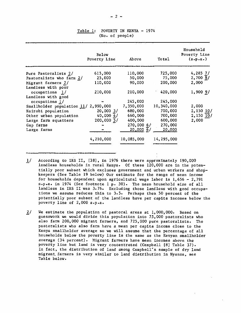
Any measure of absolute poverty is very sensitive to thepoverty line chosen. We discuss the relevant issues in this choice inAppendix 1. We have taken the Thorbecke-Crawford [90] cut-off povertylevel of 2,000 sh. p.a. per rural smallholder household as the ruralpoverty level. This has then been adjusted for rural-urban price dif-ferentials and differences in mean household size to yield the povertylines shown in the last column of Table 1. (The notes to the Tableprovide the details of their derivation.)

-2-

Table 1: POVERTY IN KENYA - 1974(No. of people)

HouseholdBelow Poverty Line

Poverty Line Above Total (s.p.a.)

Pure Pastoralists 2/ 615,000 110,000 725,000 4,285 7/Pastoralists who farm 2/ 25,000 50,000 75,000 2,700 8/Migrant farmers 2/ 110,000 90,000 200,000 2,000Landless with poor

occupations 1/ 210,000 210,000 420,000 1,900 9/Landless with good

occupations 1/ - 245,000 245,000Smallholder population 11/ 2,990,000 7,350,000 10,340,000 2,000Nairobi population 20,000 3/ 680,000 700,000 2,150 10/Other urban population 40,000 4/ 660,000 700,000 2,150 10/Large farm squatters 200,000 5/ 400,000 600,000 2,000Gap farms - 270,000 6/ 270,000Large farms - 20,000 6/ 20,000

4,210,000 10,085,000 14,295,000

1/ According to IRS II, (38], in 1976 there were approximately 190,000landless households in rural Kenya. Of these 120,000 are in the poten-tially poor subset which excluaes government and urban workers and shop-keepers (See Table 19 below) Our estimate for the range of mean incomefor households dependent upon agricultural wage labor is 1,656 - 2,791s.p.a. in 1974 (See footnote I p. 30). The mean household size of alllandless in IRS II was 3.76. Excluding those landless with good occupa-tions we assume reduces this to 3.5. Perhaps then 50 percent of thepotentially poor subset of the landless have per capita incomes below thepoverty line of 2,000 s.p.a.

2/ We estimate the population of pastoral areas at 1,000,000. Based onguesswork we would divide this population into 75,000 pastoralists whoalso farm 200,000 migrant farmers, and 725,000 pure pastoralists. Thepastoralists who also farm have a mean per capita income close to theKenya smallholder average so we will assume that the percentage of allhouseholds below the poverty line is the same as the Kenyan smallholderaverage (34 percent). Migrant farmers have mean incomes above thepoverty line but land is very concentrated (Campbell [8] Table 37).In fact, the distribution of land among Campbell's sample of dry landmigrant farmers is very similar to land distribution in Nyanza, seeTable below.

- 3 -

Table la: Land Distribution of Migrant Farmers 1976

% Population Migrant Farmers Nyanza,Smallholders

40 14.8 12.930 25.8 28.030 59.4 59.1

The poverty line among migrant farmers occurs at 77 percent of mean income.In Nyanza 55 percent of smallholders earn below 77 percent of mean income. Wewill therefore assign 55 percent of migrant farmers to the poverty group. Inthe case of pure pastoralists mean per capita income is below the poverty line.Using the distribution of cattle cited above, only 15 percent of pastoralistswould have per capita incomes above the poverty line.

3/ See Appendix 3 [39a], p. 18.

4/ Wages in other urban areas are 79% of the Nairobi mean wage. Thisfactor is then applied to the 1974 Nairobi income distribution and theresult rounded up to the nearest 10,000. The population of 'otherurban areas' is assumed to be 50% of total urban by 1974, see [39a]Appendix 3, p. 1.

5/ Thorbecke's [90] total times the proportion of the smallholderpopulation in poverty.

6/ Thorbecke's figure.

7/ Mean household size of pastoralists/mean household size ofsmallholders x smallholder poverty line = 15/7x2000=4,285.

8/ As in 7, 9.5/7 x 2,000 = 2,700.

9/ This is possibly too high given that the landless household is abouthalf the size of the smallholder household. However, prices mightbe higher for the landless than those used to estimate smallholderincome.

10/ Smallholder poverty line of 340 s.p. capita X 1.69 cost of livingdifferential X urban household size.

11/ Derived from IRS-I [331.

From this Table it can be seen that in 1974 roughly four millionpeople were poor in Kenya (out of a total population of 14.3 million), ofwhich the majority (three million) were smallholders. There were only avery small number of urban poor, namely sixty thousand.

- 4 -

It is not possible with the available data to present as completea picture of the extent of poverty (or its composition) for earlier years.However, there is data which enables us to chart trends in the incidence ofpoverty for three sub-groups of the Kenyan population, viz., smallholders inCentral Province, smallholders in Nyanza, and for Nairobi. This represents74 percent of the smallholder population in 1974, and about 50 percent of theurban population in the same year.

Table 2 provides our estimates of the proportion of the relevantpopulation in poverty for earlier years (1963 for Central Province small-holders and 1969 for Nairobi), as well as the relevant proportions for 1974(derived from Table 1).

Table 2: Trends in Absolute Poverty, 1963-74(% Population Below Poverty Line)

1963 1969 1970 1974

Smallholders (Central Province) 18.0 - - 14.6Smallholders (Nyanza) - - 28.6 28.4Nairobi - less than - less than

3% 3%

Source: Derived in Appendices 1, 2, 3 in [39a].

From this table it can be seen that the proportion of the relevant populationin absolute poverty is likely to have remained relatively constant in Nyanza,but somewhat declined in Central Province, whilst in Nairobi the incidenceof absolute poverty has been negligible.

Income, Consumption and Land Distribution

Tables 3 and 4 provide our estimates of the national distributionof income for 1974.

Table 3: The Distribution of Income in Kenya: 1974

Smallholder householdincome equivalent (s.p.a.) % Population % Income

Above 8,000 25 672,000 - 8,000 46 27Below 2,000 29 6

Source: Table 4.

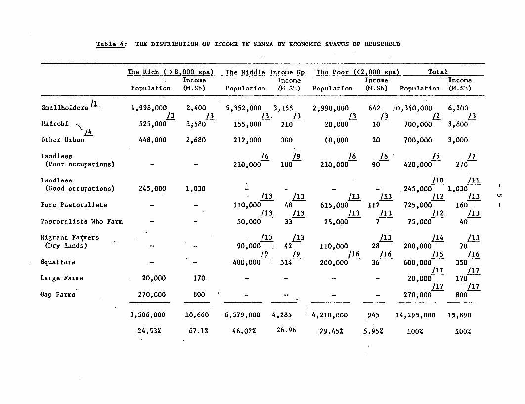
Table 4: THE DISTRIBUTION OF INCOME IN KENYA BY ECONOMIC STATUS OF HOUSEIIOLD

The Rich >8,000 spa) The Middle Income Cp The Poor (<2,000 spa) TotalIncome Income Income Income

Population (M.Sh) Population (H.Sh) Population (M.Sh) Population (M.Sh)

Smallholderas 1,998,000 2,400 5,352,000 3,158 2,990,000 642 10,340,000 6,200/3 /3 /3. /3 /3 /3 /2 /3

Nlairobi 525,000 3,580 155,000 210 20,000 10 700,000 3,800

Other Urban 448,000 2,680 212,000 300 40,000 20 700,000 3,000

Landless /6 /9 /6 /8 /5 /7(Poor occupations) - - 210,000 180 210,000 90 420,000 270

Landless - /10 /11(Good occupations) 245,000 1,030 - - - - 245,000 1,030

- /13 /13 /13 /13 /12 /13Pure Pastoralists - - 110,000 48 615,000 112 725,000 160

/13 /13 /13 /13 /12 /13Pastoralists Who Farm - - 50,000 33 25,000 7 75,000 40

Migrant Farmers /13 /13 /li /14 /13(Dry lands) - 90,000 42 110,000 28 200,000 70

/9 /9 /16 /16 /15 /16Squatters - 400,000 314 200,000 36 600,000 350

/17 117Large Fanrs 20,000 170- - - - - 20,000 170

/17 /17Gap Farms 270,000 800 ' - - - - 270,000 800

3,506,000 10,660 6,579,000 4,285 4,210,000 945 14,295,000 15,890

24,53% 67.1% 46.02% 26.96 29.45% 5.95% 100% 100%

- 6 -

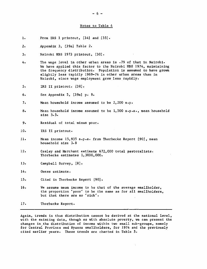
Notes to Table 4

1. From IRS I printout, [34] and [35].

2. Appendix 3, [39a] Table 2.

3. Nairobi HBS 1973 printout, (30].

4. The wage level in other urban areas is .79 of that in Nairobi.We have applied this factor to the Nairobi HBS 1974, maintainingthe frequency distribution. Population is assumed to have grownslightly less rapidly 1969-74 in other urban areas than inNairobi, since wage employment grew less rapidly.

5. IRS II printout. [38].

6. See Appendix 5, [39a] p. 9.

7. Mean household income assumed to be 2,200 s.p.

8. Mean household income assumed to be 1,500 s.p.a., mean householdsize 3.5.

9. Residual of total minus poor.

10. IRS II printout.

11. Mean income 15,935 s.p.a. from Thorbecke Report (901, meanhousehold size 3.8

12. Casley and Marchant estimate 672,000 total pastoralists.Thorbecke estimates 1,3000,000.

13. Campbell Survey, [8].

14. Guess estimate.

15. Cited in Thorbecke Report (90].

16. We assume mean income to be that of the average smallholder,the proportion 'poor' to be the same as for all smallholders,but that there are no 'rich'.

17. Thorbecke Report.

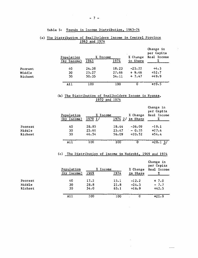
Again, trends in thus distribution cannot be derived at the national level,with the existing data, though as with absolute poverty, we can present thechanges in*the distribution of income within two small sub-groups, namelyfor Central Province and Nyanza smallholders, for 1974 and the previouslycited earlier years. These trends are charted in Table 5.

-7-

Table 5: Trends in Income Distribution, 1963-74

(a) The Distribution of Smallholders Income in Central Province1963 and 1974

Change inper Capita

Population % Income % Change Real Income(by Income) 1963 1974 in Share %

Poorest 40 24.38 18.23 -25.22 +4.3Middle 30 25.27 27.66 + 9.46 +52.7Richest 30 50.35 54.11 + 7.47 +49.9

All 100 100 0 +39.5

(b) The Distribution of Smallholders Income in Nyanza,1970 and 1974

Change inper Capita

Population % Income % Change Real Income(by Income) 1970 1/ 1974 2/ in Share %

Poorest 40 28.85 18.44 .-36.09 -19.1Middle 30 25.61 25.47 - 0.55 +27.4Richest 30 46.54 56.09 +20.52 +54.4

All 100 100 0 +28.1 3/

(c) The Distribution of Income in Nairobi, 1969 and 1974

Change inper Capita

Population % Income % Change Real Income(by Income) 1969 1974 in Share %

Poorest 40 17.2 15.1 -12.2 + 7.0Middle 30 28.8 21.8 -24.3 - 7.7Richest 30 54.0 63.1 +16.9 +42.5

All 100 100 0 +21.9

- 8-

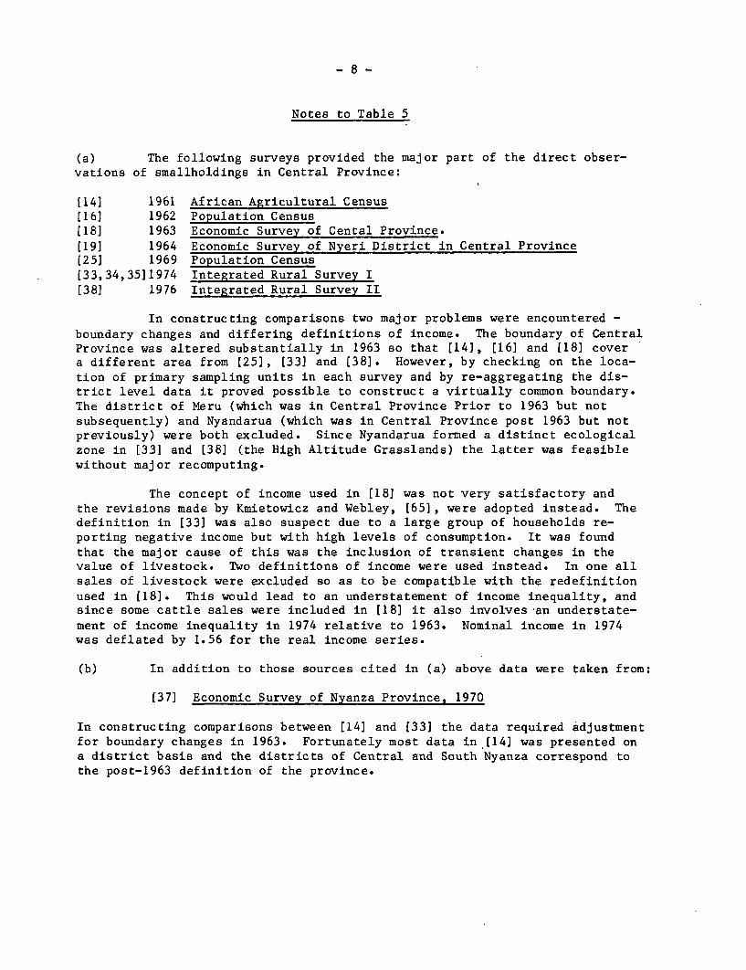
Notes to Table 5

(a) The following surveys provided the major part of the direct obser-vations of smallholdings in Central Province:

[14] 1961 African Agricultural Census[16] 1962 Population Census[18] 1963 Economic Survey of Cental Province.[19] 1964 Economic Survey of Nyeri District in Central Province[251 1969 Population Census[33,34,35]1974 Integrated Rural Survey I[38] 1976 Integrated Rural Survey II

In constructing comparisons two major problems were encountered -

boundary changes and differing definitions of income. The boundary of CentralProvince was altered substantially in 1963 so that [14], [16] and [18] covera different area from [25], [33] and [38]. However, by checking on the loca-tion of primary sampling units in each survey and by re-aggregating the dis-trict level data it proved possible to construct a virtually common boundary.The district of Meru (which was in Central Province Prior to 1963 but notsubsequently) and Nyandarua (which was in Central Province post 1963 but notpreviously) were both excluded. Since Nyandarua formed a distinct ecologicalzone in [33] and [38] (the High Altitude Grasslands) the latter was feasiblewithout major recomputing.

The concept of income used in (18] was not very satisfactory andthe revisions made by Kmietowicz and Webley, [65], were adopted instead. Thedefinition in [33] was also suspect due to a large group of households re-porting negative income but with high levels of consumption. It was foundthat the major cause of this was the inclusion of transient changes in thevalue of livestock. Two definitions of income were used instead. In one allsales of livestock were excluded so as to be compatible with the redefinitionused in [18]. This would lead to an understatement of income inequality, andsince some cattle sales were included in [18] it also involves an understate-ment of income inequality in 1974 relative to 1963. Nominal income in 1974was deflated by 1.56 for the real income series.

(b) In addition to those sources cited in (a) above data were taken from:

[37] Economic Survey of Nyanza Province, 1970

In constructing comparisons between [14] and (33] the data required adjustmentfor boundary changes in 1963. Fortunately most data in [14] was presented ona district basis and the districts of Central and South Nyanza correspond tothe post-1963 definition of the province.

-9-

1. [37], Table 1.8. This includes households reportingfor less than 10 months because the exclusion of thesehouseholds biases upwards the income estimates in theremaining tables of [37].

2. [35] Income redefined to adopt the permanent offtakeconcept of livestock income. This being that rate ofofftake which would keep constant the value of the herd.This replaced transient changes in the value of livestock.The remaining 1.3% of households still showing negativeincome were found to be farmers with government loans,anxious to demonstrate an inability to repay them. Thesehouseholds were found to have above average levels ofconsumption and were excluded from the income distri-bution data. No such households were reported in [37]so the problems of negative income did not arise.

3. This figure is unreliable for reasons given in (b) 1 and2.

(c) Derived from Household Budget Surveys [15], [30].

From Table 5 it can be seen that the distribution of income amongstthe rural sub-groups of the population has worsened; per capita real incomeamongst the lower 40 percent of the smallholder population of Central Provincewas roughly constant, whilst that of the other income classes increased sub-stantially. For Nyanza the per capita real income of the lowest 40 percentdeclined by about 19 percent between 1970 and 1974, that for the middle 30percent of smallholders rose significantly, and that for the top 30 percentincreased very substantially (about 54 percent).

For Central Province and Nyanza smallholders we can also chartchanges in the distribution of consumption (for the relevant years). Theseare shown in Table 6.

Table 6: Trends in the Distribution ofSmallholder Consumption, 1963-1974

% Population Central Province Nyanza(by household Income) 1963 1/ 1974 2/ 1970 3/ 1974 4/

Poorest 40 32.2 25.8 32.2 26.2Middle 30 24.7 28.4 30.7 29.7Richest 30 43.1 45.8 37.1 44.1

Source: 1/ and 2/ are from [18] [33,34,35]; and 3/ (35] and 4/ [37]

- 10 -

The distribution of consumption also seems to have worsened in both groups,but not as much as the distribution of income.

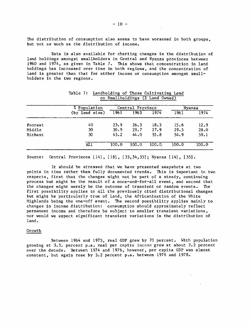
Data is also available for charting changes in the distribution ofland holdings amongst smallholders in Central and Nyanza provinces between1960 and 1974, as given in Table 7. This shows that concentration in landholdings has increased over time in both regions, and the concentration ofland is greater than that for either income or consumption amongst small-holders in the two regions.

Table 7: Landholding of Those Cultivating Landon Smallholdings (% Land Owned)

% Population Central Province Nyanza(by land size) 1961 1963 1974 1961 1974

Poorest 40 23.9 26.3 18.3 15.6 12.9Middle 30 30.9 29.7 27.9 29.5 28.0Richest 30 45.2 44.0 53.8 54.9 59.1

All 100.0 100.0 100.0O 100.0 100.0

Source: Central Provinces [14], [18], [33,34,35]; Nyanza [14], [35].

It should be stressed that we have presented snapshots at twopoints in time rather than fully documented trends. This is important in tworespects, first that the changes might not be part of a steady, continuingprocess but might be the result of a once-and-for-all event, and second thatthe changes might merely be the outcome of transient or random events. Thefirst possibility applies to all the previously cited distributional changesbut might be particularly true of land, the Africanisation of the WhiteHighlands being the one-off event. The second possibility applies mainly tochanges in income distribution: consumption should approximately reflectpermanent income and therefore be subject to smaller transient variations,nor would we expect significant transient variations in the distribution ofland.

Growth

Between 1964 and 1975, real GDP grew by 70 percent. With populationgrowing at 3.3. percent p.a. real per capita income grew at about 2.2 percentover the decade. Between 1974 and 1976, however, per capita GDP was almostconstant, but again rose by 3.2 percent p.a. between 1976 and 1978.

Per capita consumption grew at the rate of 2.5 percent p.a. overthe period 1963-74. Total wage employment between 1966 and 1975 grew atthe rate of 3.8 percent per annum, of which agricultural wage employmentgrew by only 0.44 percent per annum, and private non-agricultural employmentby 4.05 percent p.a., whilst public sector wage employment grew at 6.07percent p.a. Urban wage employment grew at the rate of 3.3 percent p.a.between 1967-76. However, this included substantial differences in growthrates in sub-periods. There was virtual stagnation till 1970, rapid growthbetween 1970 and 1974, stagnation in 1974-75, and a recovery between 1975-77.

- 12 -

II. The Characteristics of the Poor

In this chapter we provide evidence on the characteristics of thepoor in Kenya. From Table 1, it can be seen that (in descending order ofimportance) the poor are to be found amongst smallholders, pastoralists,landless, squatters, migrant farmers in dryland areas, and urban dwellers.

1. Smallholders

Thirty percent of the smallholder population in 1974 were poor.From Table 8, it can be seen that the poor smallholders have less land, lowerinputs (purchased and own produced) per acre, lower non-farm incomes, lowereducation levels, lower subsistence consumption as well as lower levels of on-farm innovation (as measured by purchased inputs) than the smallholder average.

Table 8: Characteristics of the Smallholder Poor 1/(K.shs., except percentage)

Smallholder0-999 spa 1000-1999 spa Average

Farm sales 191 586 1192Subsistence consumption 458 751 1297'Wages paid 40 46 160Purchased inputs 50 96 241Own produced inputs 13 47 84

Farm operating surplus 129 649 2081Non-farm enterprises surplus 87 170 354Other non-farm income 335 666 1217

Value of land 951 1084 1820Value of buildings 850 887 1796Value of livestock 1060 1505 2462

Total assets 3150 3954 6905Total consumption 1611 2166 3450No education (%) 83% 87% 72%

Source: [33], [34], [35].

1/ IRS coverage of smallholdings is not complete since large farm areas inwhich illegal subdivision has taken place are excluded, however itclearly ranks among the best surveys of African smallholders. A problemencountered by the survey was that some 7% of houeholds reported negativeincome during the year. On inspection these households have high levelsof both consumption and assets. Negative income is not a sign of povertyand can be attributed to two causes, households which have sufferedtransient livestock losses, and households with large loans outstandingwhich have overstated farm costs fearing that the survey was connectedwith loan repayment. In this table and our subsequent analysis of thepoverty group we have excluded the negative income group and also thosehouseholds whose income is within the band 0-2,000 s.p.a. purely due tolarge livestock losses. Our poverty group is therefore smallholders withincomes between 0 and 2,000 s.p.a. after exclusion of these groups.

- 13 -

From Table 9 which provides our estimates and those by Crawfordand Thorbecke [8a], it can be seen that smallholder poverty is not stronglyregion-specific. In no region on our estimates are less than 20 percent ormore than 50 percent of smallholders poor. (But see the note to the Table)

Table 9: Smallholder Poverty by Region, 1974

No. of Poor % Households in Re- As a % of AllRegion Households gion Who are Poor Smallholder Poor

Central 71,409 (61,000) 21.67 (18). 14.1 (16.2)Coast 21,657 (34,000) 31.00 (48) 4.3 ( 9.0)Eastern 124,100 (71,000) 35.14 (20) 24.4 (18.8)Nyanza 145,684 (85,000) 37.70 (22) 28.7 (22.6)Rift 16,869 (17,000) 18.78 (19) 3.3 ( 4.5)Western 128,073 (109,000) 50.30 (43) 25.2 (28.9)

Total 507,792 (377,000) 34.24 (25) 100.0 (100.0)

Source: [33], [34], [35], and [8a].

Note: The figures in brackets are the estimates of Crawford and Thorbecke[8a], of the percentage of households in each region who sufferfrom what they term food poverty. Their estimates differ from oursbecause they have taken account of regional price differences tooin the minimum food basket, which we have ignored for the reasonsgiven in Appendix 1. The reason why they show a much higher pro-portion of households in poverty in the Coast, is because theyestimate that their food cost index based on prices of maize andbeans were 26% higher than the national average in the Coast. Theirhousehold food poverty lines have ranged from shs 1265 in Nyanzato shs 2301 in Coast province. However, T. Kirton in an unpublishednote on [8a] has argued that they have exaggerated the cost of thereference diet, by a mistaken weighting of beans and maize in theirstandard reference diet. Secondly they have underestimated thecalorific content of maize. Taking account of these errors Kirtonfinds only 10% of Kenya smallholders in food poverty.

Using a Thiel index only 4% of the variance in household incomes is explainedby inter-regional differences. This is not necessarily an indication thatrural poverty is not location specific. Whilst regions are the appropriateunits for investigating policy-induced inequalities (being the location-specific budgeting divisions) they are not the best units for the analysis ofinequalities due to ecology. However, even when we grouped the IRS-I datainto eight ecological zones, only 10% of the variance in incomes is explainedby interzonal differences. The major explanations for smallholder poverty,is unlikely, therefore, to be found in regional or ecological differences.Nevertheless, not surprisingly, there are differences in the reasons forsmallholder poverty in the different regions. To focus on these we examine

- 14 -

the causes of smallholder poverty in greater detail for three regions: viz.Central, Nyanza, and Western provinces, which together accounted for 60percent of smallholder poverty in 1974.

These three provinces represent different stages of rural develop-ment. Thus, Central Province has had a high degreee of agricultural innova-tion (in the form of a switch to cash crops, improved livestock, hybrid maizeand a high level of purchased inputs): By contrast, Western Province has hadlittle agricultural innovation, whilst Nyanza is at an intermediate stage.

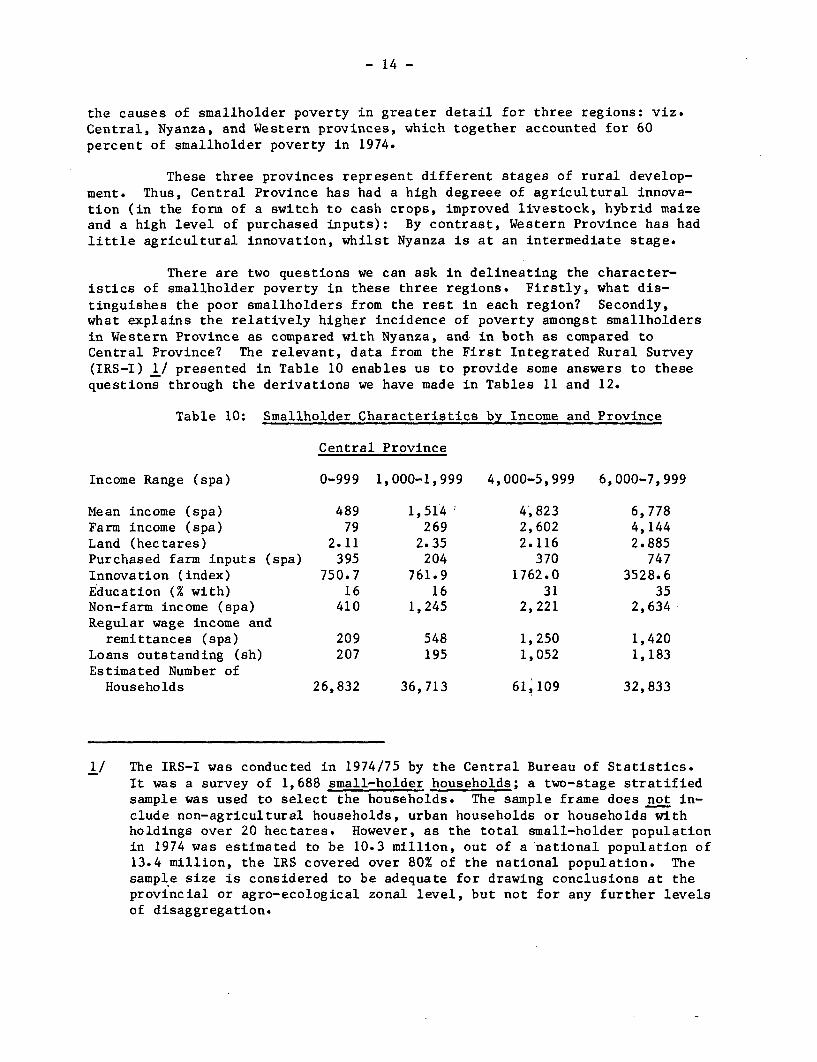
There are two questions we can ask in delineating the character-istics of smallholder poverty in these three regions. Firstly, what dis-tinguishes the poor smallholders from the rest in each region? Secondly,what explains the relatively higher incidence of poverty amongst smallholdersin Western Province as compared with Nyanza, and, in both as compared toCentral Province? The relevant, data from the First Integrated Rural Survey(IRS-I) 1/ presented in Table 10 enables us to provide some answers to thesequestions through the derivations we have made in Tables 11 and 12.

Table 10: Smallholder Characteristics by Income and Province

Central Province

Income Range (spa) 0-999 1,000-1,999 4,000-5,999 6,000-7,999

Mean income (spa) 489 1,514 4,823 6,778Farm income (spa) 79 269 2,602 4,144Land (hectares) 2.11 2.35 2.116 2.885Purchased farm inputs (spa) 395 204 370 747Innovation (index) 750.7 761.9 1762.0 3528.6Education (% with) 16 16 31 35Non-farm income (spa) 410 1,245 2,221 2,634Regular wage income and

remittances (spa) 209 548 1,250 1,420Loans outstanding (sh) 207 195 1,052 1,183Estimated Number of

Households 26,832 36,713 61,109 32,833

1/ The IRS-I was conducted in 1974/75 by the Central Bureau of Statistics.It was a survey of 1,688 small-holder households; a two-stage stratifiedsample was used to select the households. The sample frame does not in-clude non-agricultural households, urban households or households withholdings over 20 hectares. However, as the total small-holder populationin 1974 was estimated to be 10.3 million, out of a 'national population of13.4 million, the IRS covered over 80% of the national population. Thesample size is considered to be adequate for drawing conclusions at theprovincial or agro-ecological zonal level, but not for any further levelsof disaggregation.

- 15 -

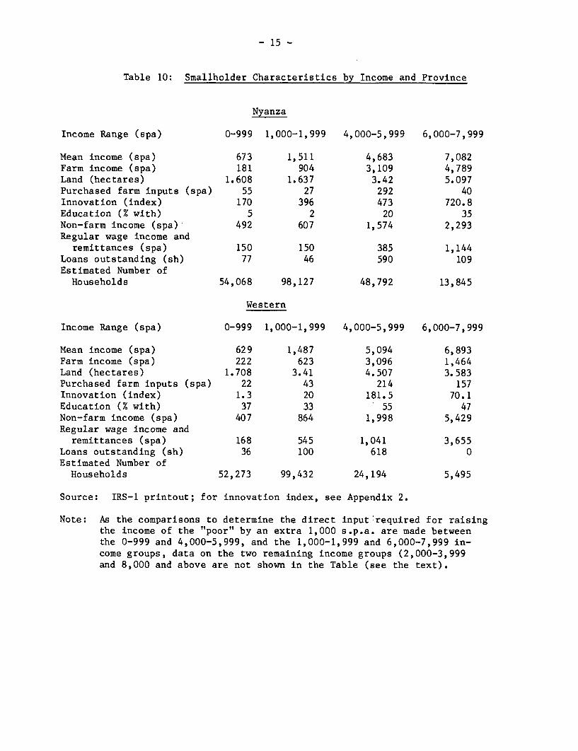
Table 10: Smallholder Characteristics by Income and Province

Nyanza

Income Range (spa) 0-999 1,000-1,999 4,000-5,999 6,000-7,999

Mean income (spa) 673 1,511 4,683 7,082Farm income (spa) 181 904 3,109 4,789Land (hectares) 1.608 1.637 3.42 5.097Purchased farm inputs (spa) 55 27 292 40Innovation (index) 170 396 473 720.8Education (% with) 5 2 20 35Non-farm income (spa) 492 607 1,574 2,293Regular wage income and

remittances (spa) 150 150 385 1,144Loans outstanding (sh) 77 46 590 109Estimated Number of

Households 54,068 98,127 48,792 13,845

Western

Income Range (spa) 0-999 1,000-1,999 4,000-5,999 6,000-7,999

Mean income (spa) 629 1,487 5,094 6,893Farm income (spa) 222 623 3,096 1,464Land (hectares) 1.708 3.41 4.507 3.583Purchased farm inputs (spa) 22 43 214 157Innovation (index) 1.3 20 181.5 70.1Education (% with) 37 33 55 47Non-farm income (spa) 407 864 1,998 5,429Regular wage income and

remittances (spa) 168 545 1,041 3,655Loans outstanding (sh) 36 100 618 0Estimated Number of

Households 52,273 99,432 24,194 5,495

Source: IRS-1 printout; for innovation index, see Appendix 2.

Note: As the comparisons to determine the direct input required for raisingthe income of the "poor" by an extra 1,000 s.p.a. are made betweenthe 0-999 and 4,000-5,999, and the 1,000-1,999 and 6,000-7,999 in-come groups, data on the two remaining income groups (2,000-3,999and 8,000 and above are not shown in the Table (see the text).

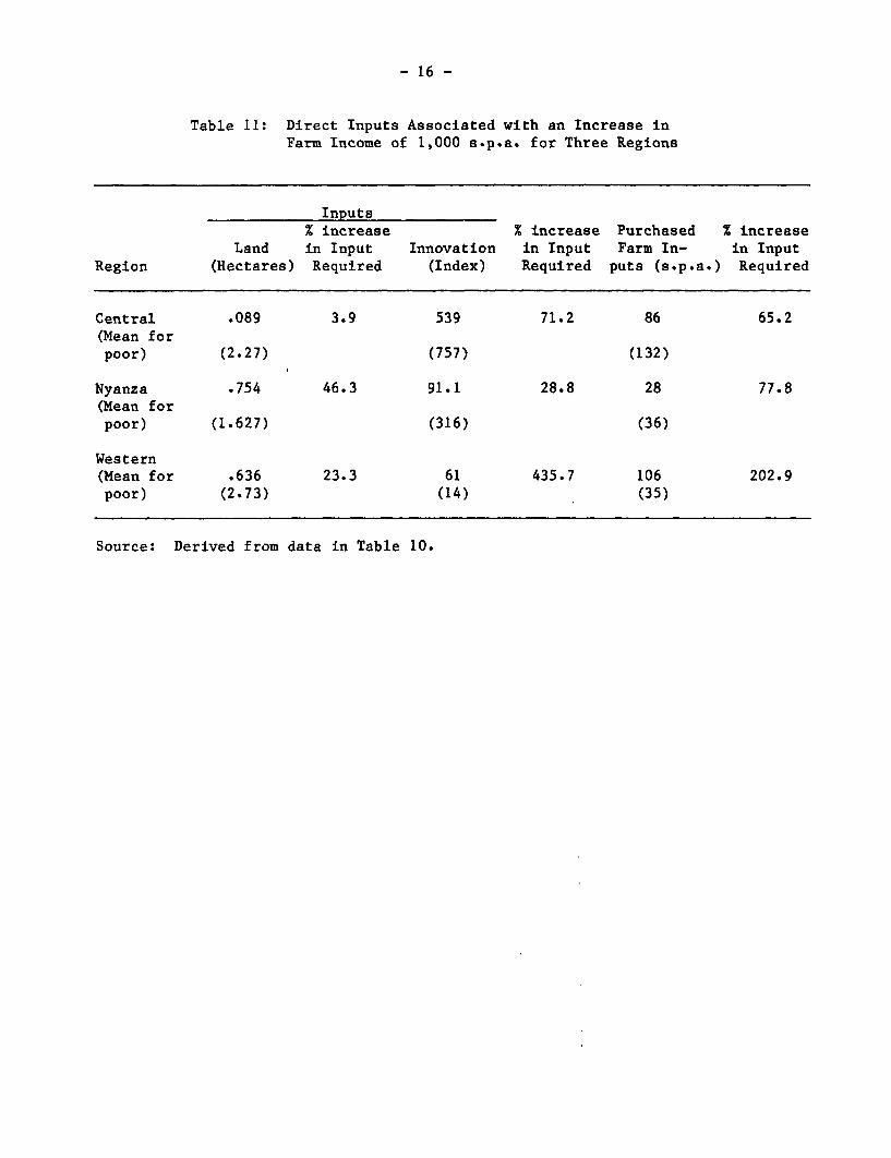
- 16 -

Table 11: Direct Inputs Associated with an Increase inFarm Income of 1,000 s.p.a. for Three Regions

Inputs% increase % increase Purchased % increase

Land in Input Innovation in Input Farm In- in InputRegion (Hectares) Required (Index) Required puts (s.p.a.) Required

Central .089 3.9 539 71.2 86 65.2(Mean forpoor) (2.27) (757) (132)

Nyanza .754 46.3 91.1 28.8 28 77.8(Mean forpoor) (1.627) (316) (36)

Western(Mean for .636 23.3 61 435.7 106 202.9poor) (2.73) (14) (35)

Source: Derived from data in Table 10.

- 17 -

Table 10 shows characteristics of small-holders in 3 provinces andby four income groups. We compare (in Tables 11 and 12) the determinantsof household incomes of two "poor" groups (those with incomes in the range0-999 spa and 1,000-1,999 spa) with those of two relatively better-offgroups (income ranges 4,000-5,999 and 6,000-7,999 spa). We then seekexplanations of the determinants of small-holder poverty by comparing theincreases in the inputs of land, an innovation index (derived in Appendix 2)and purchased farm inputs, which are jointly required to yield an extra 1,000shillings of farm income to the average poor small-holder in the region.Assuming that the relative prices of these inputs and hence the ratios oftheir marginal products are the same for every income group in the respectiveregion, variations in farm output and farm incomes will depend upon the jointvariation in these inputs accross the various income groups. Thus for eachregion we compare the levels of these inputs for the 0-999 s.p.a. incomegroup with those for the 4,000-5,999 spa group; and those for the 1,000-1,999spa group with those for the 6,000-7,999 group. It being assumed that theresulting income increase would in each case unambigously redress the povertyof the relevant "poor" group. In each of these two-way comparisons wedetermine the marginal increases in the three inputs which are required toyield an extra 1,000 shillings of farm income to each of the two poor small-holder groups. The figures for the region's average 'poor' small-holder isthen derived as the weighted average of the determinants of the two poorgroups incremental income, the weights being the number of households in thetwo respective "poor" income classes. The resulting figures are given inTable 11. 1/

1/ Thus if Y is farm income, L is land, I is innovation and P is purchasedfarm inputs, then we assume that Y=f (L, I, P) - (1)Total differentiation yields dY= fL dL + fI dI + f dP - (2)

Hence we have for an increase in farm income of 1000 shs that:

1000 = 1000 [ f dL + f dl + f dP -(3)L dY I dY p dY

Assuming that in each region small holders in the different income groupsface the same prices of the inputs, the marginal products of the inputswill ex hypothesi be the same for the different income groups in each region.It should be noted that we have no data to test this "efficiency" assumption.If it is valid, however, then given that the fi terms are region - specificparameters, we can determine the total differentials dL/dY, dI and dP/dY.

dyFrom IRS-1 we have the data in Table 10 for four sub-groups, two "poor" andtwo "rich", on the mean values of Y, L, I,P for each of the groups. De-noting poor by subscript p, and rich by subscript r, we then have

dX = Xr - XpdY Yr - Yp

for X = L, I, P. The resulting figures for the two sub-groups are thenaveraged by using the no. of households in each of the two poor sub-groupsas weights. Multiplying the resulting figures by 1,000 yields the figuresgiven in Table 11.

- 18 -

This shows that, in Central province for instance, the averagepoor smallholder has 2.27 hectares of land, uses purchased farm inputs of132 sh. p.a., and has an innovation index (based on a composite of the adop-tion of coffee, tea, and improved livestock per farm) of 757. To generate anextra 1,000 sh. of farm income (and assuming unchanged productivities of theseinputs), this average poor smallholder would need an extra 0.089 hectares ofland, plus an extra 86 sh. worth of purchased farm inputs, and an increase inits innovation index of 539.

By contrast in Nyanza, incremental farm income requires (in absoluteterms) much more extra land, and much less innovation or increases in purchasedfarm inputs than in Central and Western provinces (except for the innovationrequirement being lower in Western province). The latter is clearly an inter-mediate case between Central and Nyanza Provinces. Thus we can conclude thatsmallholder poverty in Central Province is primarily associated with a failureto innovate relative to the better off farmers in the region, whilst that inNyanza is also associated with their low levels of land holdings. In WestrnProvince all three factors are of importance, but relative to the mean levelsof the inputs on the average poor smallholder farm, the levels of innovationand purchased farm inputs need to be doubled to generate an extra 1,000 sh.of farm income, whilst the land area has to be increased by only 20 percent.These conclusions are also supported by the relative strengths of the simplecorrelation between land size and smallholder income for the three regionswhich we ran on IRS-1 data. The correlation coefficient is significant atthe one percent level for Nyanza, at only the 5 percent level for WesternProvince, and is not significant even at the 10 percent level for CentralProvince. 1/

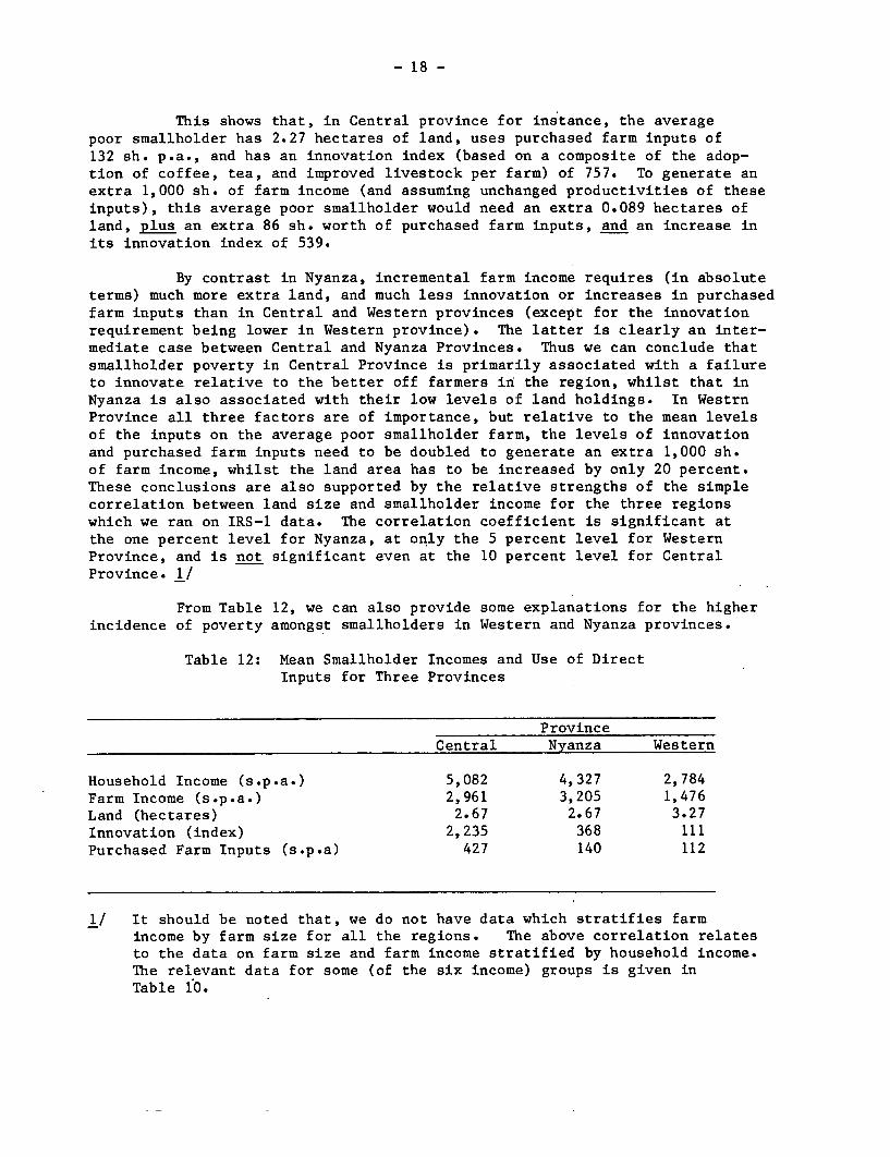
From Table 12, we can also provide some explanations for the higherincidence of poverty amongst smallholders in Western and Nyanza provinces.

Table 12: Mean Smallholder Incomes and Use of DirectInputs for Three Provinces

ProvinceCentral Nyanza Western

Household Income (s.p.a.) 5,082 4,327 2,784Farm Income (s.p.a.) 2,961 3,205 1,476Land (hectares) 2.67 2.67 3.27Innovation (index) 2,235 368 111Purchased Farm Inputs (s.p.a) 427 140 112

1/ It should be noted that, we do not have data which stratifies farmincome by farm size for all the regions. The above correlation relatesto the data on farm size and farm income stratified by household income.The relevant data for some (of the six income) groups is given inTable 10.

- 19 -

Prima facie one would expect that differences in the average incomes of allsmallholders in the three regions would be correlated with the differencesin the incidence of poverty amongst their smallholders. From Table 12, itcan be seen that the mean household income in Nyanza is about 20 percentless than in Central Province, whilst that in Western Province is nearlyhalf that in Central Province. But whereas, in Western Province both thefarm and non-farm components of household incomes are lower than their re-spective values for Central Province, in Nyanza mean farm income levels ofthe average smallholder are higher than in Central Province, and the dif-ference in the mean household incomes in the two provinces is explicableentirely in terms of differences in non-farm income. Thus, we would expectthat differences in the relative incidence of poverty in the three provinceswould be related to the determinants of lower non-farm incomes in Nyanzarelative to Central Province, and to both lower farm and non-farm incomes inWestern Province. For the latter, from the evidence on the mean inputs ofinnovation, purchased farm inputs and labor on the average smallholder farm,it appears that all these are lower than those on a smaller average farm sizein the other two provinces.

The characteristics of smallholder poverty identified above, arein terms of the determinants of farm income, and the relative contributionof farm income to total household income. Of the determinants of farm in-come the differences in the size of land-ownership are in a sense structuralvariables, for which we provide no further explanation and take them as givenin what follows. For the two other inputs, innovation and the purchase offarm inputs, we need to explain differences in their values across dif-ferent smallholder farms. Two variables which are likely to be importantdeterminants of these inputs are education and financing.

In addition to loans, non-farm income is likely to be an impor-tant source of funds to break any financial constraint on financing bothinnovation as well as purchased farm inputs. Thus, for instance, if theaverage poor smallholder were to increase his purchased farm inputs tothe level of the mean for all smallholders, the financial burden wouldrequire a reduction in household consumption of about 25 percent if met outof current income. Hence the importance of the financial constraint onpurchases of farm inputs as well as the capital expenditure (including the'waiting' involved in the relatively long gestation periods) associatedwith innovation. Thus, we need to look at differences in education, loansand non-farm income as providing further (and deeper) explanations of thepoverty of smallholders in the three regions. Table 13 provides thenecessary data, on loans and non-farm income.

- 20 -

Table 13: Direct and Indirect Farm Inputs for Three Provinces

Direct Inputs Indirect InputsPurchased Non-Farm Loans

Innovation Farm Inputs Income Outstanding(Index) (s.p.a.) (s.p.a.) (Sh)

Mean for all Smallholders

Central 2,235 427 2,121 991Nyanza 368 140 1,122 247Western 111 112 1,308 144

Incremental 1,000 s.p.a. ofFarm Income

Central 539 86 488 284Nyanza 91 28 414 67Western 61 106 3,330 155

From Table 13 it can be seen that the levels of loans cum non-farmincome are correlated with the levels of innovation and purchased farm in-puts for smallholders in both the Central and Western Provinces. The Tablealso suggests that, as we have already found that innovation and/or purchaseof farm inputs were important determinants of poverty amongst smallholders inCentral and Western Provinces, the availability of loans and increases in non-farm income would be relatively more important determinants of small-holderpoverty within these regions, than in Nyanza (where the inequalities of land-holdings were an additional determinant of smallholder poverty).

As regards the effects of differences in the levels of non-farmincomes cum loans, as between the three regions, in explaining the differingregional incidence of small-holder poverty, from Table 13 it appears that thedifferences in the levels of innovation and purchased farm inputs are corre-lated with those in non-farm income cum loans. Thus it. seems that besidesthe importance of differences in land-holdings for Nyanza province, the majorcorrelate of smallholder poverty is the availability of financing. It shouldbe noted that for Nyanza, the low non-farm income component is a direct causeof smallholder poverty (see Table 12). What the above arguments have soughtto establish is that non-farm income cum loans are also indirectly (throughtheir high correlation with the levels of innovation and purchased inputs)important correlates of smallholder poverty in Central and Western Provinces.

- 21 -

Furthermore, we would expect that the loans component of the avail-ability of finance for smallholders would be closely correlated with non-farmincome (as it is), with the level of non-farm income determining both theability as well as the willingness of smallholders to borrow. The risk ofborrowing without an adequate non-farm income is that land offered as col-lateral might have to be sold. That this is not an idle fear for smallholdersin Kenya, is borne out by the experience of smallholders on the Lugari settle-ment scheme. On this scheme, smallholders were forced to take out loans tofinance both purchases of current inputs as well as the purchases of the free-hold of the land. By 1977, 80 percent of the smallholders had forfeited theirland because of loan defaults. Similarly, lenders in Kenya look to the non-farm income of smallholders as a source of servicing any loans, when extendingcredit. For example, in a recent survey of smallholders with loans for farm-ing purposes taken out from the Kenya Commercial Bank, David and Wyeth [41]found that 70% received income from wage employment. The survey coveredNyanza, Western, Rift, Eastern and Central Provinces. Applying the samecoverage and weights to IRS-I data 1/ yields the result that only 9.7% ofsmallholder household heads received income from wage employment, only 20.5%undertaking any activity other than operating their own holding. Hence,smallholders taking out loans for farming purposes are heavily biased towardsthose with above average non-farm incomes. Further support for this is givenin Table 14 which shows that most farmers taking out loans regarded theirsalary as more important than their farm incomes. 2/

1/ Table 6.4 of [33], using teaching, government and urban employmentas a proxy for wage employment.

2/ If we had this data classified by farm size, which we do not, afirm test of the hypothesis would have been possible.

- 22 -

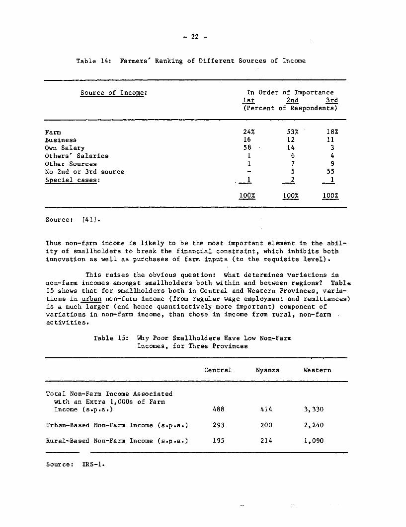
Table 14: Farmers' Ranking of Different Sources of Income

Source of Income: In Order of Importance1st 2nd 3rd(Percent of Respondents)

Farm 24% 53% 18%Business 16 12 11Own Salary 58 14 3Others' Salaries 1 6 4Other Sources 1 7 9No 2nd or 3rd source - 5 55Special cases: 1 2 1

100% 100% 100%

Source: [41].

Thus non-farm income is likely to be the most important element in the abil-ity of smallholders to break the financial constraint, which inhibits bothinnovation as well as purchases of farm inputs (to the requisite level).

This raises the obvious question: what determines variations innon-farm incomes amongst smallholders both within and between regions? Table15 shows that for smallholders both in Central and Western Provinces, varia-tions in urban non-farm income (from regular wage employment and remittances)is a much larger (and hence quantitatively more important) component ofvariations in non-farm income, than those in income from rural, non-farmactivities.

Table 15: Why Poor Smallholders Have Low Non-FarmIncomes, for Three Provinces

Central Nyanza Western

Total Non-Farm Income Associatedwith an Extra 1,000s of FarmIncome (s.p.a.) 488 414 3,330

Urban-Based Non-Farm Income (s.p.a.) 293 200 2,240

Rural-Based Non-Farm Income (s.p.a.) 195 214 1,090

Source: IRS-1.

- 23 -

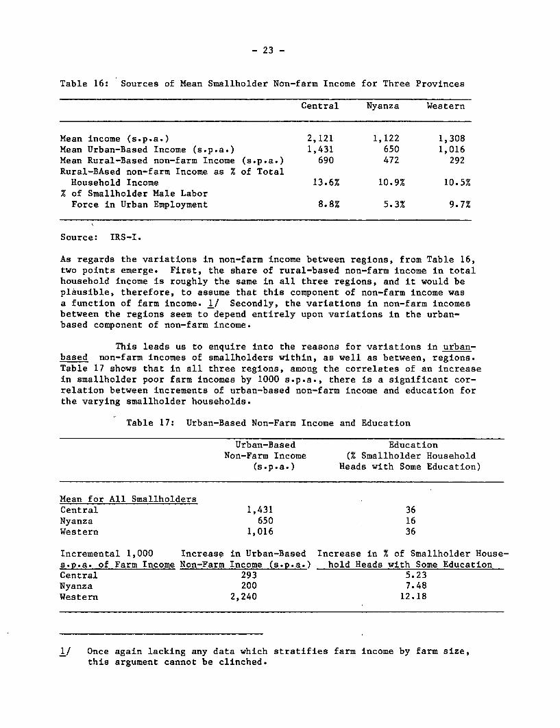
Table 16: Sources of Mean Smallholder Non-farm Income for Three Provinces

Central Nyanza Western

Mean income (s.p.a.) 2,121 1,122 1,308Mean Urban-Based Income (s.p.a.) 1,431 650 1,016Mean Rural-Based non-farm Income (s.p.a.) 690 472 292Rural-BAsed non-farm Income as % of Total

Household Income 13.6% 10.9% 10.5%% of Smallholder Male Labor

Force in Urban Employment 8.8% 5.3% 9.7%

Source: IRS-I.

As regards the variations in non-farm income between regions, from Table 16,two points emerge. First, the share of rural-based non-farm income in totalhousehold income is roughly the same in all three regions, and it would beplausible, therefore, to assume that this component of non-farm income wasa function of farm income. 1/ Secondly, the variations in non-farm incomesbetween the regions seem to depend entirely upon variations in the urban-based component of non-farm income.

This leads us to enquire into the reasons for variations in urban-based non-farm incomes of smallholders within, as well as between, regions.Table 17 shows that in all three regions, among the correlates of an increasein smallholder poor farm incomes by 1000 s.p.a., there is a significant cor-relation between increments of urban-based non-farm income and education forthe varying smallholder households.

Table 17: Urban-Based Non-Farm Income and Education

Urban-Based EducationNon-Farm Income (% Smallholder Household

(s.p.a.) Heads with Some Education)

Mean for All SmallholdersCentral 1,431 36Nyanza 650 16Western 1,016 36

Incremental 1,000 Increase in Urban-Based Increase in % of Smallholder House-s.p.a. of Farm Income Non-Farm Income (s.p.a.) hold Heads with Some EducationCentral 293 5.23Nyanza 200 7.48Western 2,240 12.18

1/ Once again lacking any data which stratifies farm income by farm size,this argument cannot be clinched.

- 24 -

From this same table it appears that the same correlation holds between themeans of the regional smallholder urban-based non-farm income and the pro-portion of the smallholder population with education.

Thus, through the above chain of argument, we seem to have arrivedat the importance of varying levels of education as the major indirect in-fluence which explains variations in smallholder household incomes. Thechain runs through the effects of education on urban-based non-farm income,and thence on total non-farm income which in turn enables any financialbottlenecks in the purchase of farm inputs, as well as other means forinnovating, to be broken, leading to higher farm incomes. However, it mayalso be thought that education would also directly effect the levels offarm incomes through its effects on inducing innovation. From Tables 10and 18 it appears that though there is a positive correlation between edu-cation and innovation levels within each region, there is no correlationin the same variables between regions.

Table 18: Innovation and Education

EducationInnovation (% Smallholder Household

(Index) Heads with some Education)

Mean for All Smallholders

Central 896 36Nyanza 89 16Western 62 36

Thus Western Province has the most educated smallholder population but thelowest level of innovation amongst our three regions. So it might not beimplausible to conclude that the within region correlation between educationand innovation is due to the indirect effect of education on innovationthrough the chain which runs via the effects of education on the levels ofurban-based non-farm income, rather than any direct effects of education oninnovation levels.

- 25 -

2. The Landless, Outmigrants and Pastoralists

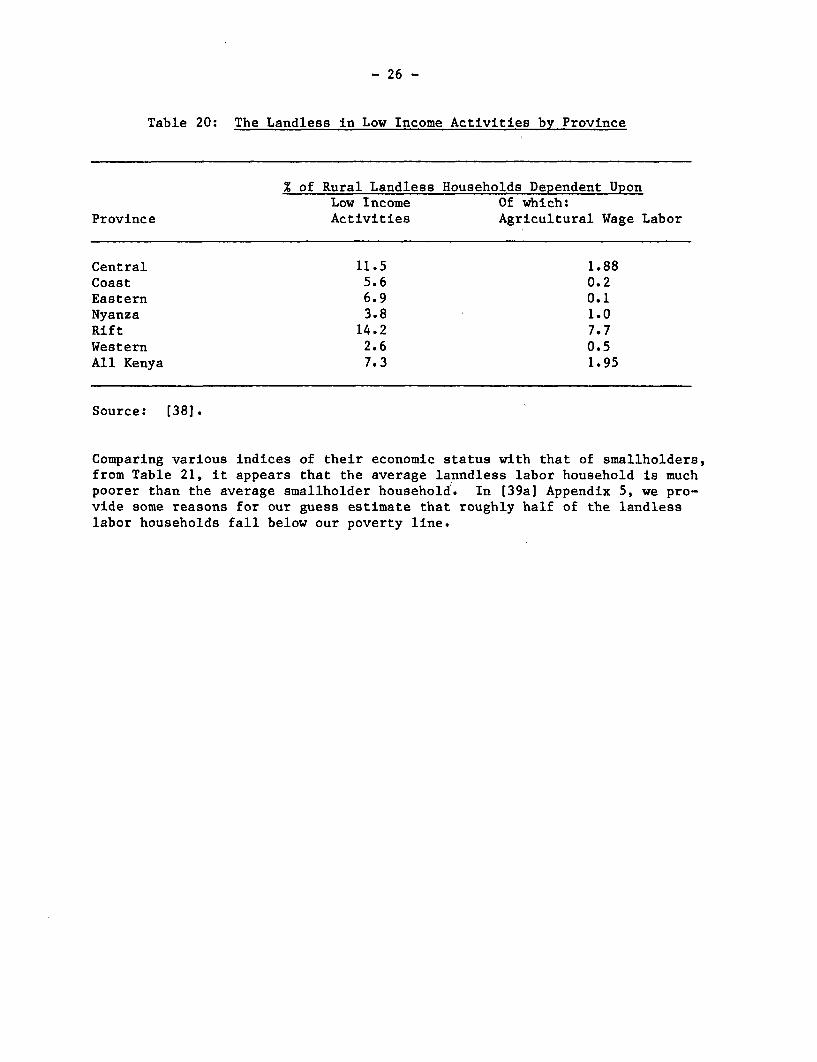
About 11 percent of all rural households are landless, but not allof the landless are poor. As Table 19 shows, if the categories of "urbanemployment", "shopkeepers", and "government workers" are taken to be occupa-tions where income levels are likely to be well above the poverty line, we areleft with roughtly 7.3 percent of the rural population which is landless andlikely to be poor.

Table 19: The Rural Landless by Occupation in 1976

Activity %

Agricultural Laborer 17.1Government Worker 27.5Shopkeeper/Trader a/ 8.5Production, Transport and Crafts .7.2Urban Employment 3.7Other Employment 29.4No employment Reported 6.25

Total 100.00

Source: (38]

Note: a/ These exclude petty traders, as a study among the poorin Machakos [79], found that petty traders had thesame social characteristics as agricultural laborers.

Of this subset of the potentially poor, we have virtually noinformation on any of the other occupations besides agriculturallaborers, who, however, account for 60 percent of the populationin this subset (excluding the category other employment - see[39a] Appendix 5).

From Table 20 it appears that most of the landless agri-cultural laborers (65 percent) are in the Rift Valley.

- 26 -

Table 20: The Landless in Low Income Activities by Province

% of Rural Landless Households Dependent UponLow Income Of which:

Province Activities Agricultural Wage Labor

Central 11.5 1.88Coast 5.6 0.2Eastern 6.9 0.1Nyanza 3.8 1.0Rift 14.2 7.7Western 2.6 0.5All Kenya 7.3 1.95

Source: (38].

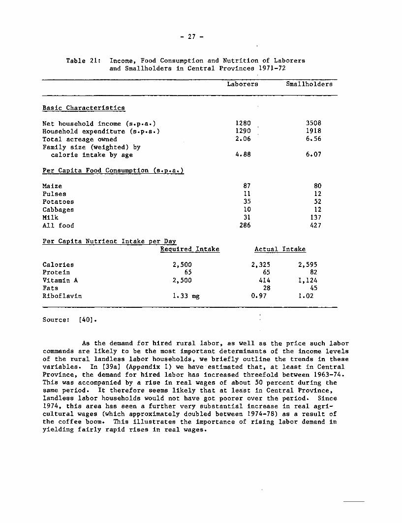
Comparing various indices of their economic status with that of smallholders,from Table 21, it appears that the average lanndless labor household is muchpoorer than the average smallholder household. In (39a] Appendix 5, we pro-vide some reasons for our guess estimate that roughly half of the landlesslabor households fall below our poverty line.

- 27 -

Table 21: Income, Food Consumption and Nutrition of Laborersand Smallholders in Central Provinces 1971-72

Laborers Smallholders

Basic Characteristics

Net household income (s.p.a.) 1280 3508Household expenditure (s.p.a.) 1290 1918Total acreage owned 2.06 6.56Family size (weighted) by

calorie intake by age 4.88 6.07

Per Capita Food Consumption (s.p.a.)

Maize 87 80Pulses 11 12Potatoes 35 52Cabbages 10 12Milk 31 137All food 286 427

Per Capita Nutrient Intake per DayRequired Intake Actual Intake

Calories 2,500 2,325 2,595Protein 65 65 82Vitamin A 2,500 414 1,124Fats 28 45Riboflavin 1.33 mg 0.97 1.02

Source: [40].

As the demand for hired rural labor, as well as the price such laborcommands are likely to be the most important determinants of the income levelsof the rural landless labor households, we briefly outline the trends in thesevariables. In [39a] (Appendix 1) we have estimated that, at least in CentralProvince, the demand for hired labor has increased threefold between 1963-74.This was accompanied by a rise in real wages of about 50 percent during thesame period. It therefore seems likely that at least in Central Province,landless labor households would not have got poorer over the period. Since1974, this area has seen a further very substantial increase in real agri-cultural wages (which approximately doubled between 1974-78) as a result ofthe coffee boom. This illustrates the importance of rising labor demand inyielding fairly rapid rises in real wages.

- 28 -

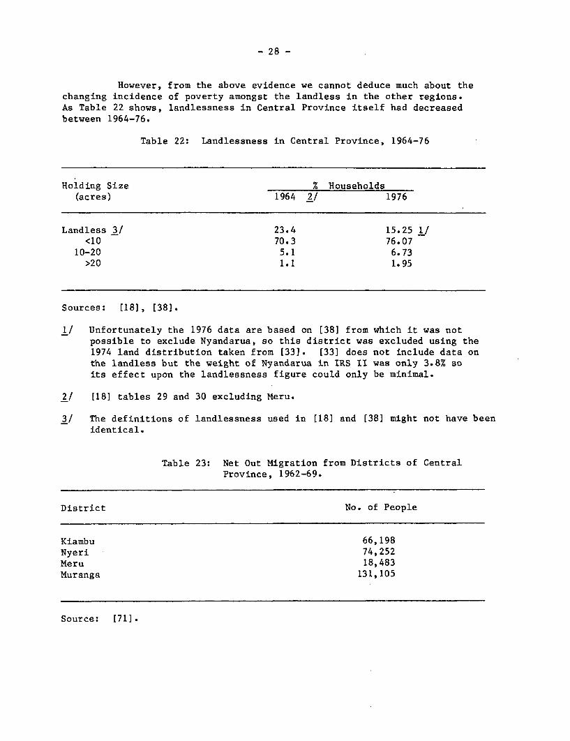
However, from the above evidence we cannot deduce much about thechanging incidence of poverty amongst the landless in the other regions.As Table 22 shows, landlessness in Central Province itself had decreasedbetween 1964-76.

Table 22: Landlessness in Central Province, 1964-76

Holding Size % Households(acres) 1964 2/ 1976

Landless 3/ 23.4 15.25 1/<10 70.3 76.07

10-20 5.1 6.73>20 1.1 1.95

Sources: [18], [38).

1/ Unfortunately the 1976 data are based on (38] from which it was notpossible to exclude Nyandarua, so this district was excluded using the1974 land distribution taken from [33]. [33] does not include data onthe landless but the weight of Nyandarua in IRS II was only 3.8% soits effect upon the landlessness figure could only be minimal.

2/ [18] tables 29 and 30 excluding Meru.

3/ The definitions of landlessness used in [18] and [38] might not have beenidentical.

Table 23: Net Out Migration from Districts of CentralProvince, 1962-69.

District No. of People

Kiambu 66,198Nyeri 74,252Meru 18,483Muranga 131,105

Source: [71].

- 29 -

This is primarily the result of outmigration from the province (see Table23). Given our evidence on the increased land concentration in the province(Table 7), the decrease in landlessness could not be due to any redistributionof land amongst the province's rural population. Thus any provincial trendsin landlessness are likely to be misleading, because most of the potentiallandless in each of the provinces have outmigrated to newer lands, where theycease to be landless. It is therefore more useful to incorporate the out-migrants as part of the subset of potentially landless groups.

Most of the potentially landless have migrated to three broad areasof "newer" lands. These are (a) to the settlement schemes, which were ex-hausted during the 1960s; (b) to large farms as squatters; and (c) to drylands, previously occupied by.pastoralists. (In addition there is a rela-tively small number of landless migrants to urban areas, but as we show inChapter 3, rural-urban migration is not linked to landlessness).

In deriving the characteristics of the outmigrants, and hence ofthe potentially landless (which includes the actual landless in each province),we need some explanation of the causes of landlessness in Kenya, as well astheir income earning potential in their new locations.

There are four main causes of landlessness in Kenya. From a surveyof Machokos, and a study by Migot-Adholla for Nyanza [71), [72], [79], itappears that first, privatistation of land, leading to legal disputes andthe ensuing court decisions, have led to landlessness. Second, land sales tofinance school fees or repay loans, are also important causes of landlessness.Third, squatters who leave the holdings which they farm (due for instance toa drought) cannot return as they have no rights to the land. Fourth, land-lessness results from widowhood and divorce as old social norms are broken.Not only are wives deprived of their husband's lands following a divorce, buttheir children too are often disinherited.

The resulting landlessness is the major cause' of rural-ruralmigration. 1/ Of the possible alternative locations for these migrants, the

1/ In a survey of migrants to Machakios 53 percent had previously been land-less and a further 27 percent had owned less than one acre. Rural migra-tion is neither education nor age biased. Rural-to-rural out-migrationhas been a feature of Central Province, Western Province and parts ofNyanza. For example, in 1962-69 the district of Kagmega experiencednet out-migration of 310,927. Mbithi [68] considers western Kenya to besuffering from "rural involution" in which the frustrated landless resortto delinquency such as crop burning in addition to out-migration. Rurallandless out-migrants do not go to the towns but either purchase landelsewhere, become squatters, or move to marginal lands. Narok, forexample, has experienced very substantial in-migration, especially fromCentral Province.

- 30 -

settlement schemes ceased offering any outlet after the late 1960s. We havevery little information on those who have chosen to squat on large farms.That leaves those migrants who have settled on the dry lands of the pastoral-ists. This move does lead to some increase in the migrants' household in-comes. We have estimated that the average income in 1976 of landless agri-cultural labor households was within the range of 1,700 to 2,500 sh. p.a. 1/From a survey by Campbell, [8], the mean income of dryland migrant farmers in1976 was 2,590 sh. p.a. This would still leave a number of these drylandmigrants below the poverty line. In Table 1 we estimate that roughly half ofdryland migrant households were below the poverty line in 1976.

The movement of the potentially landless into the drylands, hasbrought them into conflict with the pastoralists, another of our povertygroups in Kenya. The migrants compete with the pastoralists for land.

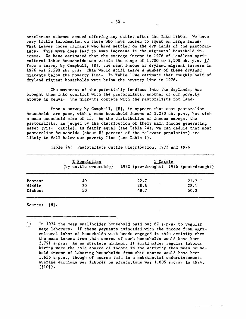
From a survey by Campbell, (8], it appears that most pastoralisthouseholds are poor, with a mean household income of 3,270 sh. p.a., but witha mean household size of 15. As the distribution of income amongst thepastoralists, as judged by the distribution of their main income generatingasset (viz. cattle), is fairly equal (see Table 24), we can deduce that mostpastoralist households (about 85 percent of the relevant population) arelikely to fall below our poverty line (see Table 1).

Table 24: Pastoralists Cattle Distribution, 1972 and 1976

% Population % Cattle(by cattle ownership) 1972 (pre-drought) 1976 (post-drought)

Poorest 40 22.7 21.7Middle 30 28.6 28.1Richest 30 48.7 50.2

Source: (8].

1/ In 1974 the mean smallholder household paid out 67 s.p.a. to regularwage laborers. If these payments coincided with the income from agri-cultural labor of households with heads engaged in this activity thenthe mean income from this source of such households would have been2,791 s.p.a. As an absolute minimum, if smallholder regular laborerhiring were the sole source of income in the activity then mean house-hold income of laboring households from this source would have been1,656 s.p.a., though of course this is a substantial understatement.Average earnings per laborer on plantations was 1,885 s.p.a. in 1974,([10]).

- 31 -

3. The Urban Poor

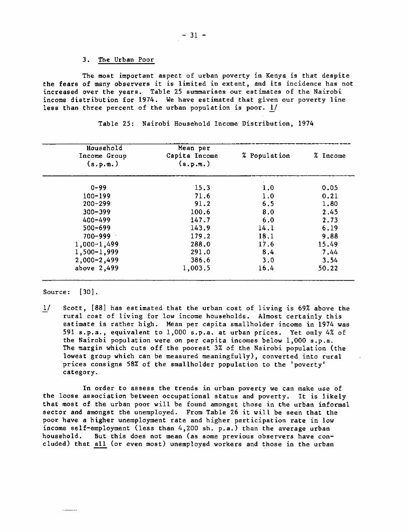
The most important aspect of urban poverty in Kenya is that despitethe fears of many observers it is limited in extent, and its incidence has notincreased over the years. Table 25 summarises our estimates of the Nairobiincome distribution for 1974. We have estimated that given our poverty lineless than three percent of the urban population is poor. 1/

Table 25: Nairobi Household Income Distribution, 1974

Household Mean perIncome Group Capita Income % Population % Income

(s.p.m.) (s.p.m.)

0-99 15.3 1.0 0.05100-199 71.6 1.0 0.21200-299 91.2 6.5 1.80300-399 100.6 8.0 2.45400-499 147.7 6.0 2.73500-699 143.9 14.1 6.19700-999 179.2 18.1 9.88

1,000-1,499 288.0 17.6 15.491,500-1,999 291.0 8.4 7.442,000-2,499 386.6 3.0 3.54above 2,499 1,003.5 16.4 50.22

Source: [30].

1/ Scott, [88] has estimated that the urban cost of living is 69% above therural cost of living for low income households. Almost certainly thisestimate is rather high. Mean per capita smallholder income in 1974 was591 s.p.a., equivalent to 1,000 s.p.a. at urban prices. Yet only 4% ofthe Nairobi population were on per capita incomes below 1,000 s.p.a.The margin which cuts off the poorest 3% of the Nairobi population (thelowest group which can be measured meaningfully), converted into ruralprices consigns 58% of the smallholder population to the 'poverty'category.

In order to assess the trends in urban poverty we can make use ofthe loose association between occupational status and poverty. It is likelythat most of the urban poor will be found amongst those in the urban informalsector and amongst the unemployed. From Table 26 it will be seen that thepoor have a higher unemployment rate and higher participation rate in lowincome self-employment (less than 4,200 sh. p.a.) than the average urbanhousehold. But this does not mean (as some previous observers have con-cluded) that all (or even most) unemployed workers and those in the urban

- 32 -

informal sector are poor. Thus in [39a] Appendix 3, we derive estimatesof the "poor" on the basis of a poverty line (which is roughly twice thenational poverty line) amongst the unemployed, and those in the urban in-formal sector in 1974. We find that even with this much higher povertyline, 67 percent of the unemployed are above the poverty line, as comparedwith 78 percent of all urban households. This suggests that there is onlya very loose correlation between unemployment and urban poverty.

Table 26: Mean and Poor Nairobi Households by Activity, 1974

Poor All

3.6 4.4 Household size40% 40% % in labour force29% 16% % unemployment rate16% 4% % low income self-employment

Source: [30].

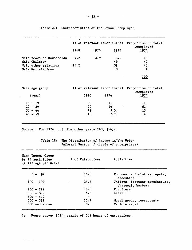
Furthermore, the average urban "poor" household has 1.44 members inthe labor force as compared with 1.76 for all urban households and 2.2 fornon-poor urban households. This implies that if we exclude the householdhead, the number of dependents in the labor force is much lower for "poor"urban households. If urban poverty and unemployment were closely related,we would thus expect to find a preponderance of heads of households amongstthe unemployed (or conversely a relatively smaller proportion of dependentsamongst the unemployed). From table 27, it is clear that this is not thecase for urban Kenya. Most of the unemployed are young dependents, and asthe poor households have only 12 percent of all the urban dependent laborforce, whilst dependents account for 33 percent of urban employment, it is areasonable inference that most of these dependent unemployed are not poor.

- 33 -

Table 27: Characteristics of the Urban Unemployed

(% of relevant labor force) Proportion of TotalUnemployed

1968 1970 1974 1974

Male heads of Households 4.2 4.9 3.9 19Male Children 49 40Male other relations 15.2 39 40Male No relations 3 1

100

Male age group (% of relevant labor force) Proportion of TotalUnemployed

(year) 1970 1974 1974

16 - 19 30 11 1120 - 29 20 19 6230 - 44 12 3.3. 1345 - 59 10 7.7 14

Source: For 1974 [30], for other years ILO, [56].

Table 28: The Distribution of Income in-the UrbanInformal Sector 1/ (heads of enterprises)

Mean Income Groupby 14 activities % of Enterprises Activities(shillings per week)

0 - 99 16.5 Footwear and clothes repair,shoeshine

100 - 199 34.7 Tailors, footwear manufacture,charcoal, barbers

200 - 299 18.5 Furniture300 - 399 5.6 Retail400 - 499 _500 - 599 16.1 Metal goods, restaurants600 and above 8.6 Vehicle repair

1/ House survey [54], sample of 502 heads of enterprises.

- 34 -

As regards the informal sector, Table 28 shows that, contrary tothe received view of this being a homogenous low income sector, the distribu-tion of income in this sector in 1977 was bi-modal, with the population inthe sector roughly equally divided between richer entrepreneurs and poorerworkers. The House survey also shows that, entrepreneurs' average incomewas roughly 27,600 sh. p.a., well above any conceivable urban poverty line!The wage-earners average income was 1,850 sh. p.a., which would put themwell below our national poverty line.

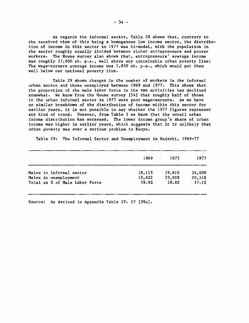
Table 29 shows changes in the number of workers in the informalurban sector and those unemployed between 1969 and 1977. This shows thatthe proportion of the male labor force in the two activities has declinedsomewhat. We know from the House survey [54] that roughly half of thosein the urban informal sector in 1977 were poor wage-earners. As we haveno similar breakdown of the distribution of income within this sector forearlier years, it is not possible to say whether the 1977 figures representany kind of trend. However, from Table 5 we know that the ovrall urbanincome distribution has worsened. The lower income group's share of urbanincome was higher in earlier years, which suggests that it is unlikely thaturban poverty was ever a serious problem in Kenya.

Table 29: The Informal Sector and Unemployment in Nairobi, 1969-77

1969 1973 1977

Males in informal sector 18,115 19,616 24,000Males in unemployment 19,622 23,928 20,518Total as % of Male Labor Force 19.8% 18.8% 17.1%

Source: As derived in Appendix Table IV. 17 [39a].

- 35 -

III. Poverty and Growth: Rural-Urban Interactions

We have presented a statistical snapshot of the poor in the lastchapter. In this chapter we provide an account of the ways in which thepattern and rate of growth have effected the levels and composition of povertyin Kenya. From the last two chapters, it is clear that, there are three setsof 'events' in Kenya in the past decade which need explanation. The first,is the nature and determinants of smallholder innovation, which has been veryrapid by African standards, but whose uneven spread in large part accounts forthe existing smallholder poverty (the largest curent poverty group in Kenya).Secondly, the pattern of growth has led to an increased concentration in landholdings. The sources of this concentration, as well as its effects on theincidence of poverty will have to be examined. Thirdly, we need to explain anon-event, namely that despite the fears of many observers in the early 1970sthere has been no dramatic increase in urban poverty, and its expected corre-lates, the levels and rate of urban unemployment, and the size of the urbaninformal sector.

Our major thesis (which will hopefully emerge) in this chapter isthat all these three 'events' can be explained in terms of some specificrural-urban interactions. In the process we also hope to show the relation-ship between urban growth and rural poverty - redressal. We have shown inChapter II, that the major explanation of differential rates of innovationamongst smallholders lies in their differential access to urban-based non-farm income. In turn differences in the latter are dependent upon differen-tials in education. We begin by trying to provide some causal explanationsfor these links.

1. Migration, Education and Innovation

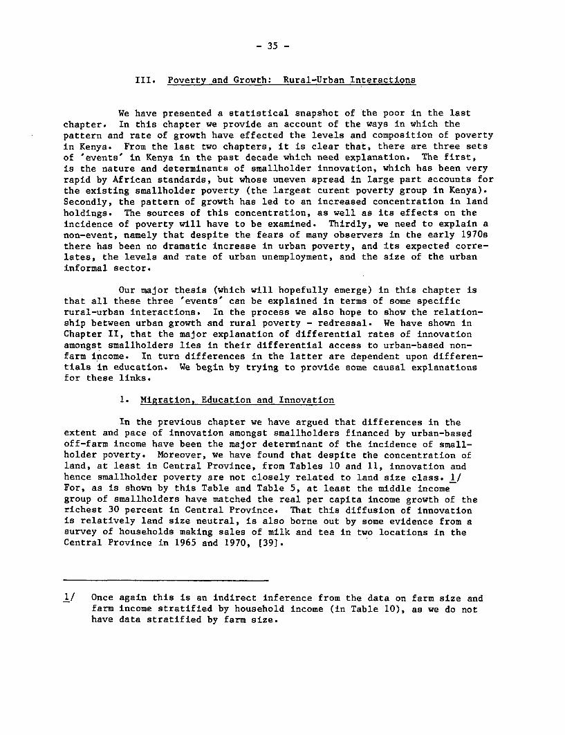
In the previous chapter we have argued that differences in theextent and pace of innovation amongst smallholders financed by urban-basedoff-farm income have been the major determinant of the incidence of small-holder poverty. Moreover, we have found that despite the concentration ofland, at least in Central Province, from Tables 10 and 11, innovation andhence smallholder poverty are not closely related to land size class. 1/For, as is shown by this Table and Table 5, at least the middle incomegroup of smallholders have matched the real per capita income growth of therichest 30 percent in Central Province. That this diffusion of innovationis relatively land size neutral, is also borne out by some evidence from asurvey of households making sales of milk and tea in two locations in theCentral Province in 1965 and 1970, [39].

1/ Once again this is an indirect inference from the data on farm size andfarm income stratified by household income (in Table 10), as we do nothave data stratified by farm size.

- 36 -

Table 30: Frequency Distribution of Households Earning Incomefrom Sales of Milk and Tea in the Majutu Districtof Central Province - 1965-1970

1) Sub Region - Gatei

Percentage of Relevant Households inEach Income Group in 1970

Per Household Per Household Sales in 1970 Total No. of Householdsin All Income Groups in

Sales in 1965 (sh) Exits 0-500 500-2000 Over-2000 1965

Entrants 0 55 39 6 360-50 2 33 51 15 81500-2000 36 63 27Over 2000 100 8

Source: [39].

2) Sub Location - Gaikuyu

Percentage of Relevant Households inEach Income Group in 1970

Per Household Per Household Sales in 1970Total No. of Households

Sales in 1965 (sh) Exits 0-500 500-2000 Over-2000 in 1965

Entrants 0 63 34 2 900-500 3 22 54 21 78500-2000 42 58 38Over 2000 8 92 13

Source: [39].

- 37 -

Table 30 shows the changes in the percentage of households withindifferent classes of the value of milk and tea sales, between 1965 and 1970.Thus for instance for the first sub-location, of the new entrants since 1965,55 percent were in the 0-500 sh. sales class in 1970. Similarly of thehouseholders who had sales of between 0-500 sh. in 1965, only 33 percentremained in the same sales class in 1970, 51 percent having moved into thehigher sales class of 500-2,000 and 15 percent into that over 2,000 sh.Table 30, therefore, shows that of the households in all the sales classes in1965, a substantial portion had succeeded in markedly raising their salesinto higher sales classes. However, only 18 percent of farm households inCentral Province in 1974 were growing tea. Moveover, from Table 31 mean landholding size in the two regions of the surveyed households was not very large.Hence it would seem likely that the increased sales from milk and tea foreach sales group (in 1965) would not be confined to the large farms. As theoverall growth in income from milk and tea sales in both sub-locations wasabout 19 percent, it would thus appear that there has been substantial dif-fusion of the benefits from the expansion in those income generating activi-ties, but that these effects have probably been confined to the relativelylarger amongst the middle income land size groups. Hence, it would seem thatit is the relatively greater diffusion of new income opportunities amongstthe middle income rural households in Central Province, which would explaintheir maintenance of real per capita income growth rates on a par with thosein higher income groups.

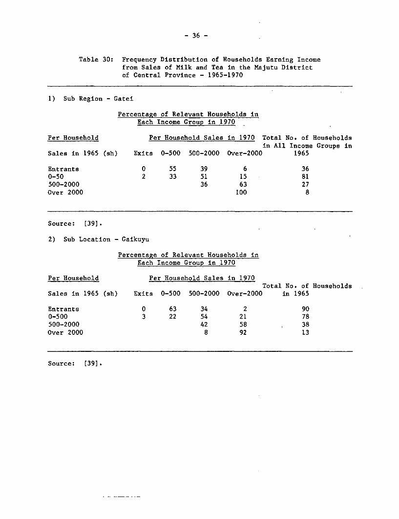
This conclusion is strengthened by the evidence from the same surveysummarised in Table 31. This provides estimates of the Gini coefficient ofcash income from sales of tea and milk of the survey households. It showsthat the distribution of income from sales of tea and milk had become moreequal in both sublocations between 1965 and 1970. This means that the house-holds which had started with the smaller sales in 1965 had experienced themore rapid growth in sales.

- 38 -

Table 31: Mean Landholding Size and Gini Coefficient of Cash Incomefrom Sales of Tea and Milk per Survey Farm Household

Central ProvinceGini Coefficient Size of Landholding

Survey Household1965 1970 (acres)

Sublocation

Gatei 0.62 0.50 3.8Gaikuyu 0.62 0.56 6.5

Source: [391.

Where non-farm incomes are high enough, smallholders ootsde._ .entralProvince too, will adopt improved farming. In Western Province--those tarmetrwhose total incomes exceeds 8,000 spa are comparable with the mean householderin Central Province in terms of farm improvements - and radically better thanthe mean smallholder in Western Province (see Table 32).

Table 32: A Comparison of Smallholder Innovation in Western andCentral Provinces

Smallholder mean WesternWestern Central > 8,000 spa

Purchased farm inputs (s.p.a.) 112 427 718Innovation (index) 62 896 768

We have argued that it is the urban-based off-farm income componentof smallholder household income which is likely to be the most important deter-minant of innovation. In turn it is the educational status of smallholderhousehold members willing and able to migrate to the towns which is likely tobe the most important determinant of the size of their urban-based off-farmincome. Thus Momanyi, [77], compared two rival sub-clans in South Nyanza.One had invested in education, the other had not. (The reason for this wasthat schools take up land and the more powerful sub-clan had used its powerto locate the schools on the land of the rival sub-clan). The sub-clan whichacquired education was then able to get jobs in the local town (Kisii) andthis money was used to purchase improved livestock and to switch into cashcrops - especially coffee. All political power still lies with the unedu-cated sub-clan but their economic fortunes have diverged dramatically fromthose of the educated sub-clan.

- 39 -

We thus need to examine the links between education, migration andsmallholder innovation. Table 33 provides data on the educational charac-teristics of rural-urban migrants for the period 1964-77. This shows thatmigrants have always been better educated, and are becoming more so overthe years. They are better educated relative to both the rural smallholderpopulation as well as rural-rural migrants. The latter's educational charac-teristics are the same as those of the rural population. 1/ However, rural-urban migrants have lower levels of education than the urban population, andare concentrated amongst those with primary education.

Table 33: Rural-Urban Migrants and Smallholders by Education

Male Migrants to Nairobi Male SmallholdersEducation 1964-68 1969-77 Aged over 20 (1974)

None (%) 10.8 - (1) 58.1Primary (%) 55.2 52.1 36.0Secondary I - III (%) 11.1 20.5 5.9Secondary IV - VI (%) 22.9 27.4 -

(1) Net out-migration

Source: Derived from [84], [36], [28], (27], [26], [74], as described in[39a] Appendix 3.

In Table 34 we provide our estimates (derived in [39a] Appendix 4)on the changing urban demand and supply balances of labor differentiated byeducational status between 1969-77. This shows that most of the unskilledlabor in the urban sector is provided by migrants with primary education.Moreover, as the bulk of unskilled jobs (from this Table) are in the urbanformal sector (with only seven percent of the incremental unskilled urbanemployment between 1969-77 being in the urban informal sector), it wouldappear that the bulk of rural-urban migrants seek and find wage employmentin the urban organised sector.

1/ See [71] and (72].

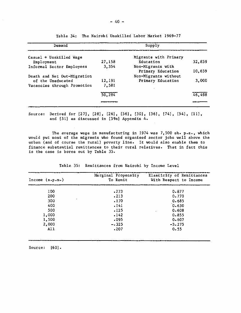
- 40 -

Table 34: The Nairobi Unskilled Labor Market 1969-77

Demand Supply

Casual + Unskilled Wage Migrants with PrimaryEmployment 27,158 Education 32,839

Informal Sector Employees 3,354 Non-Migrants withPrimary Education 10,659

Death and Net Out-Migration Non-Migrants withoutof the Uneducated 12,191 Primary Education 3,000

Vacancies through Promotion 7,581

50,284 46,498

Source: Derived for (27], [28], [26], [56], [30], (36], [74], [54], (11],and [31] as discussed in [39a] Appendix 4.

The average wage in manufacturing in 1974 was 7,500 sh. p.a., whichwould put most of the migrants who found organised sector jobs well above theurban (and of course the rural) poverty line. It would also enable them tofinance substantial remittances to their rural relatives. That in fact thisis the case is borne out by Table 35.

Table 35: Remittances from Nairobi by Income Level

Marginal Propensity Elasticity of RemittancesIncome (s.p.m.) To Remit With Respect to Income

100 .273 0.877200 .213 0.770300 .170 0.685400 .141 0.630500 .125 0.608

1,000 .142 0.8551,500 .095 0.6072,000 -.325 -3.275All .207 0.55

Source: [60].

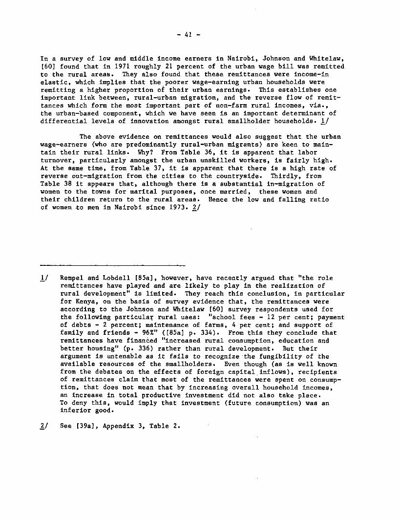
- 41 -

In a survey of low and middle income earners in Nairobi, Johnson and Whitelaw,[60] found that in 1971 roughly 21 percent of the urban wage bill was remittedto the rural areas. They also found that these remittances were income-inelastic, which implies that the poorer wage-earning urban households wereremitting a higher proportion of their urban earnings. This establishes oneimportant link between, rural-urban migration, and the reverse flow of remit-tances which form the most important part of non-farm rural incomes, via.,the urban-based component, which we have seen is an important determinant ofdifferential levels of innovation amongst rural smallholder households. 1/

The above evidence on remittances would also suggest that the urbanwage-earners (who are predominantly rural-urban migrants) are keen to main-tain their rural links. Why? From Table 36, it is apparent that laborturnover, particularly amongst the urban unskilled workers, is fairly high.At the same time, from Table 37, it is apparent that there is a high rate ofreverse out-migration from the cities to the countryside. Thirdly, fromTable 38 it appears that, although there is a substantial in-migration ofwomen to the towns for marital purposes, once married, these women andtheir children return to the rural areas. Hence the low and falling ratioof women to men in Nairobi since 1973. 2/

1/ Rempel and Lobdell [85a], however, have recently argued that "the roleremittances have played and are likely to play in the realization ofrural development" is limited. They reach this conclusion, in particularfor Kenya, on the basis of survey evidence that, the remittances wereaccording to the Johnson and Whitelaw (60] survey respondents used forthe following particular rural uses: "school fees - 12 per cent; paymentof debts - 2 percent; maintenance of farms, 4 per cent; and support offamily and friends - 96%" ([85a] p. 334). From this they conclude thatremittances have financed "increased rural consumption, education andbetter housing" (p. 336) rather than rural development. But theirargument is untenable as it fails to recognize the fungibility of theavailable resources of the smallholders. Even though (as is well knownfrom the debates on the effects of foreign capital inflows), recipientsof remittances claim that most of the remittances were spent on consump-tion, that does not mean that by increasing overall household incomes,an increase in total productive investment did not also take place.To deny this, would imply that investment (future consumption) was aninferior good.

2/ See [39a], Appendix 3, Table 2.

- 42 -

Table 36: Urban Wage Labor Turnover

Length of Stay in JobSource Type of Labor (years)

Ministry of Labor 1971 Non-Agricultural Wage[76] Labor 3.5 (Mean

IBRD Labor Force Survey Nairobi Private Sector 4.4 (Median)1968 [89] Nairobi Public Sector 4.0 (Median)

ILO Survey 1972 [561 All Urban 5.0 (Median)

% Quitting in Last12 months

ILO Survey 1972 Non-Agricultural SkilledWorkers 11.5

Non-Agricultural UnskilledWorkers 16.7

CBS Survey 1977 [31] Nairobi Informal Sector 8.9

Table 37: Rural-Urban and Urban-Rural Migration, 1973-74 1/

(% Annual Rates) 2/Male Females

Rural to Nairobi 6.1 11.0Nairobi to Rural 3.0 4.7Rural to Other Urban 3.9 5.2Other Urban to Rural 2.1 3.1

1/ Data source is [27].

2/ As a percentage of the urban population.

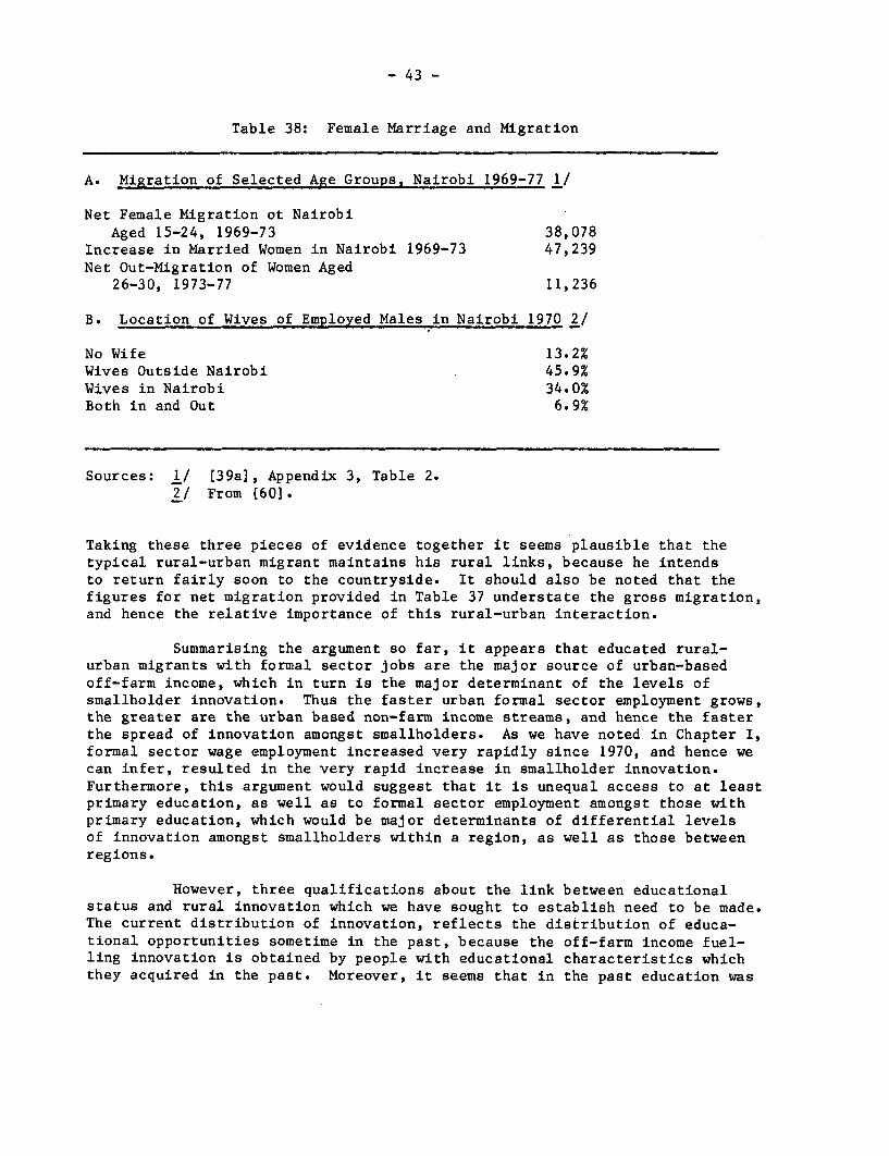
- 43 -

Table 38: Female Marriage and Migration

A. Migration of Selected Age Groups, Nairobi 1969-77 1/

Net Female Migration ot NairobiAged 15-24, 1969-73 38,078

Increase in Married Women in Nairobi 1969-73 47,239Net Out-Migration of Women Aged

26-30, 1973-77 11,236

B. Location of Wives of Employed Males in Nairobi 1970 2/

No Wife 13.2%Wives Outside Nairobi 45.9%Wives in Nairobi 34.0%Both in and Out 6.9%

Sources: 1/ [39a], Appendix 3, Table 2.2/ From (60].

Taking these three pieces of evidence together it seems plausible that thetypical rural-urban migrant maintains his rural links, because he intendsto return fairly soon to the countryside. It should also be noted that thefigures for net migration provided in Table 37 understate the gross migration,and hence the relative importance of this rural-urban interaction.

Summarising the argument so far, it appears that educated rural-urban migrants with formal sector jobs are the major source of urban-basedoff-farm income, which in turn is the major determinant of the levels ofsmallholder innovation. Thus the faster urban formal sector employment grows,the greater are the urban based non-farm income streams, and hence the fasterthe spread of innovation amongst smallholders. As we have noted in Chapter I,formal sector wage employment increased very rapidly since 1970, and hence wecan infer, resulted in the very rapid increase in smallholder innovation.Furthermore, this argument would suggest that it is unequal access to at leastprimary education, as well as to formal sector employment amongst those withprimary education, which would be major determinants of differential levelsof innovation amongst smallholders within a region, as well as those betweenregions.

However, three qualifications about the link between educationalstatus and rural innovation which we have sought to establish need to be made.The current distribution of innovation, reflects the distribution of educa-tional opportunities sometime in the past, because the off-farm income fuel-ling innovation is obtained by people with educational characteristics whichthey acquired in the past. Moreover, it seems that in the past education was

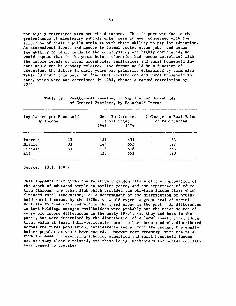
- 44 -

not highly correlated with household income. This in part was due to thepredominance of missionary schools which were as much concerned with thesalvation of their pupil's souls as with their ability to pay for education.As educational levels and access to formal sector urban jobs, and hencethe ability to remit funds to the countryside, are highly correlated, wewould expect that in the years before education had become correlated withthe income levels of rural households, remittances and rural household in-come would not be closely related. The former would be a function ofeducation, the latter in early years was primarily determined by farm size.Table 39 bears this out. We find that remittances and rural household in-come, which were not correlated in 1963, showed a marked correlation by1974.

Table 39: Remittances Received in Smallholder Householdsof Central Province, by Household Income

Population per Household Mean Remittances % Change in Real ValueBy Income (Shillings) of Remittances

1963 1974

Poorest 40 122 459 122Middle 30 144 555 127Richest 30 113 676 253All 126 553 160

Source: [331, [18].

This suggests that given the relatively random nature of the composition ofthe stock of educated people in earlier years, and the importance of educa-tion (through the urban link which provided the off-farm income flows whichfinanced rural innovation), as a determinant of the distribution of house-hold rural incomes, by the 1970s, we would expect a great deal of socialmobility to have occurred within the rural areas in the past. As differencesin land holdings amongst smallholders were probably not the major source ofhousehold income differences in the early 1970's (as they had been in thepast), -but were determined by the distribution of a 'new' asset, viz., educa-tion, which at least intra-regionally seems to have been randomly distributedacross the rural population, considerable social mobility amongst the small-holder population would have ensued. However more recently, with the rela-tive increase in fee-paying schools, education and rural household incomeare now very closely related, and these benign mechanisms for social mobilityhave ceased to operate.

- 45 -

Secondly, access to urban formal sector wage employment is likelybe unequal because of the relative distance of the various rural areas

:om the fastest growing urban centre, namely Nairobi. Thus between 1969-77,there were 70,000 extra jobs created in Nairobi, but less than 2,000 inKisumu (the local urban centre for Nyanza and Western Province). Thus,whereas the educated smallholders in Central Province had a fairly closefast growing urban centre to fuel their off-farm income increases, similaropportunities were limited for the equivalent smallholder population ofNyanza and Western Province. They would have to migrate a much further dis-tance to participate in the fast growing Nairobi economy. Because of therelatively greater distance, one would also expect that, the migrants inNairobi from Nyanza and Western Province would find it more difficult tovisit their smallholdings as often as migrants from Central Province, andperhaps they would not be able to use their urban-based off-farm income aseffectively for rural innovation.

The third qualification concerns our neglect so far of the deter-minants of poverty in Coast province and to question whether, in line withour hypothesised rural-urban interactions, the Mombassa labor market playedthe same role for Coast small-holders as Nairobi did for Central province infuelling on-farm innovation. First, from Table 9, it will be seen that,though on our estimates the incidence of poverty amongst Coast small holdersis higher than in Central Province (but lower than in most other provincesapart from Rift), as a proportion of the total number of poor small holdersCoast province accounts for only 4% of the Kenyan total. Thus in thenational context, poverty in Coast province is of marginal significance.Secondly, from Table 40 it will be seen that given the ecology of thisprovince, the indices of innovation we have derived for the other provinces(based on improved livestock, coffee and trees) are irrelevant for Coastprovince. There is virtually no improved livestock and no coffee or teagrown in the province. Coconuts and cashew are the cash crops, but we donot have any way of deriving an innovation index from these which would becomparable with that for the other provinces. Thirdly, for ecologicalreasons it is likely that the agricultural potential of this province ispoor. This is borne out by the evidence in Tables 41-and-42. From theformer Table, it will be seen that, remittance income forms the largestproportion of household income for Coast small-holders. By contrast farmincome is a low (25%) percentage, and of the same order of magnitude asremittances, of total household income. This is not surprising given therelatively poor agricultural potential of this area (see World Bank [96]p's 453 - 470). By contrast as Table 42 shows, the Coast small holdershave a very high level of income from trading and home crafts as comparedwith the other provinces. We would therefore conjecture that, the verysubstantial remittances in the Caost province (besides providing increasesin consumption for small-holder families) have been probably channeled intothe above non-farm activities. Finally, it is again likely that the basisof these large remittances, was the rapid growth of urban jobs in Mombassa,which increased by 23,497 between 1969-77. This represented a 41% increasein urban jobs in Mombassa compared to a 43% increase in Nairobi, duringthis period.

- 46 -

Table 40: Smallholder Characteristics for Coast Province

Innovation Regular Percentage PurchasedIncome Cashew Coconut Farm Employment Remit- with Farm Loans No. ofGroup Trees Trees L.S.U. Income Income tances Education Inputs Outstanding Households(spa) (No) (No) (spa) (spa) (spa) (spa) (Shs)

0-999 0.0 3.31 0 -282 29 387 3.2 77 0 5,306

1000-1999 9.48 10.43 0 195 88 540 9.4 18 0 15,439

4000-5999 20.33 16.84 0.047 874 817 1,352 25.5 51 499 14,347

6000-7999 5.98 1.68 0 2,500 1,775 1,214 26.0 32 544 4,015

8000 & above 48.16 83.65 0 9,392 1,064 1,332 21.8 24 0 3,640

Source: IRS-I (tapes).

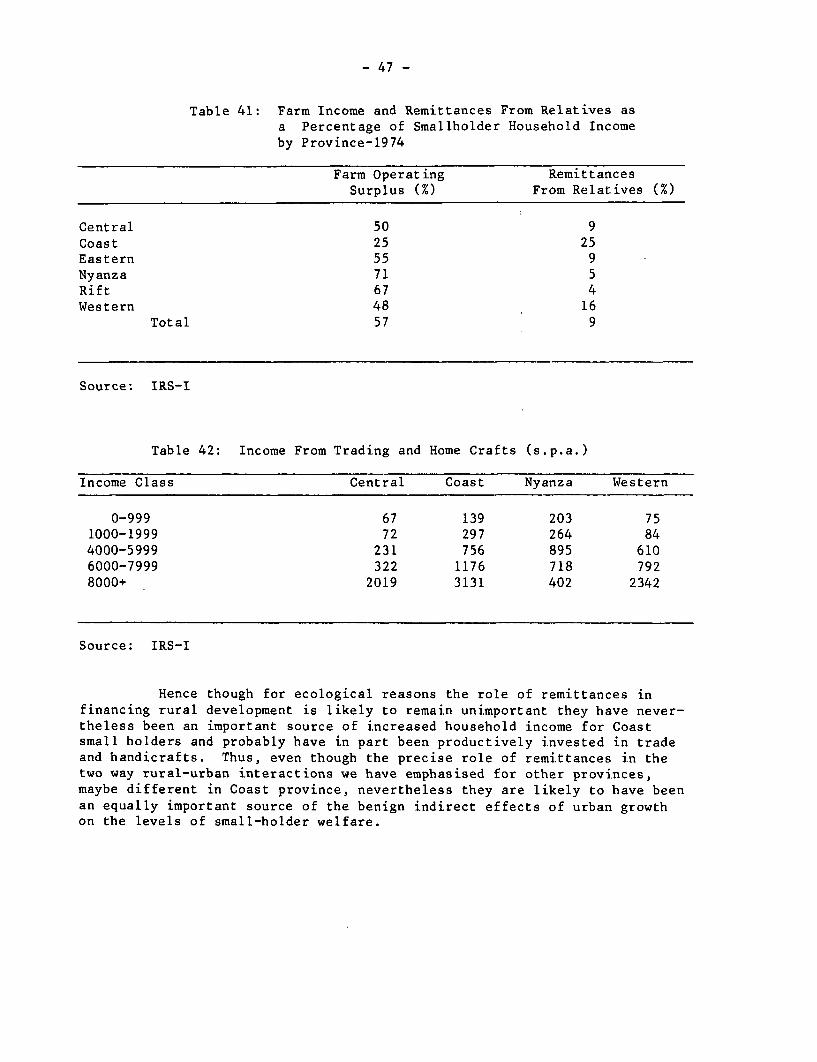
- 47 -

Table 41: Farm Income and Remittances From Relatives asa Percentage of Smallholder Household Incomeby Province-1974

Farm Operating RemittancesSurplus (%) From Relatives (%)

Central 50 9Coast 25 25Eastern 55 9Nyanza 71 5Rift 67 4Western 48 16

Total 57 9

Source: IRS-I

Table 42: Income From Trading and Home Crafts (s.p.a.)

Income Class Central Coast Nyanza Western

0-999 67 139 203 751000-1999 72 297 264 844000-5999 231 756 895 6106000-7999 322 1176 718 7928000+ 2019 3131 402 2342

Source: IRS-I

Hence though for ecological reasons the role of remittances infinancing rural development is likely to remain unimportant they have never-theless been an important source of increased household income for Coastsmall holders and probably have in part been productively invested in tradeand handicrafts. Thus, even though the precise role of remittances in thetwo way rural-urban interactions we have emphasised for other provinces,maybe different in Coast province, nevertheless they are likely to have beenan equally important source of the benign indirect effects of urban growthon the levels of small-holder welfare.

- 48 -

We hope therefore to have provided some evidence to suggest thatthere are important indirect links between the growth of the urban sector,and the rate and levels of rural innovation and more generally of rural devel-opment. Moreover, these links provide a deeper explanation of the changingextent and incidence of smallholder poverty through the mechanisms identifiedabove.

In addition, however, the same rural-urban interactions also haveimplications for the incidence of poverty amongst the landless laborers, andthe rural-rural outmigrants, and thence on the pastoralists (the other majorpoverty groups in Kenya). As shown in Chapter II, the major determinant ofpoverty amongst the landless laborers (and hence their propensity to migrateto the dry lands, and/or to become squatters), is the availability of remu-nerative work in the major agricultural regions. Both the level of demandfor rural hired labor, and its relationship with the given supply, willdetermine the rural wage rate, which in turn will determine the income levelsof rural landless labor households.

The demand for rural hired labor (from both the landless and small-holder households, who each supply roughly half of the hired labor in Kenyanagriculture (see Table 43)) is effected both by trends in innovation as wellas in land concentration. Keeping land concentration and land area constant,we have estimated that in Central Province, between 1963-74, total small-holder labor demand increased by 2.4 percent p.a., with the demand for hiredlabor rising by 2.3 percent p.a., as a result of innovation, which was measuredby the changes in cropping patterns, type of livestock and the balance betweenlivestock and crops (see [39a] Appendix 1 for details). This increased demandfor hired labor in the Province was associated with an increase of about 50percent in real rural wages during this period. This would certainly haveraised the incomes of landless laborers in the region. Thus, we can concludethat the smallholder farm innovation financed by urban remittances, would havereduced the incidence of poverty not only amongst smallholders, but alsoamongst the landless. This, of course, assumes that this innovation did notlead to any further concentration of land, which could be expected to havecountervailing depressive effects on the demand for labor. We turn to thisissue in the next section. At this stage we can conclude that through therural-urban mechanisms described in this section, rapid growth in the demandfor urban unskilled labour could (in the absence of land concentration) simul-taneously raise the income levels of rural smallholders, as well as those ofrural landless laborers.

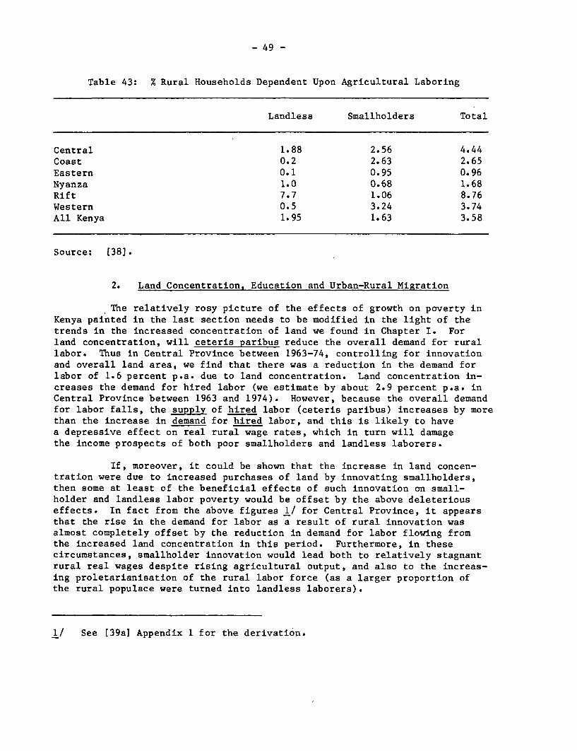
- 49 -

Table 43: % Rural Households Dependent Upon Agricultural Laboring

Landless Smallholders Total

Central 1.88 2.56 4.44Coast 0.2 2.63 2.65Eastern 0.1 0.95 0.96Nyanza 1.0 0.68 1.68Rift 7.7 1.06 8.76Western 0.5 3.24 3.74All Kenya 1.95 1.63 3.58

Source: (38].

2. Land Concentration, Education and Urban-Rural Migration

The relatively rosy picture of the effects of growth on poverty inKenya painted in the last section needs to be modified in the light of thetrends in the increased concentration of land we found in Chapter I. Forland concentration, will ceteris paribus reduce the overall demand for rurallabor. Thus in Central Province between 1963-74, controlling for innovationand overall land area, we find that there was a reduction in the demand forlabor of 1.6 percent p.a. due to land concentration. Land concentration in-creases the demand for hired labor (we estimate by about 2.9 percent p.a. inCentral Province between 1963 and 1974). However, because the overall demandfor labor falls, the supply of hired labor (ceteris paribus) increases by morethan the increase in demand for hired labor, and this is likely to havea depressive effect on real rural wage rates, which in turn will damagethe income prospects of both poor smallholders and landless laborers.

If, moreover, it could be shown that the increase in land concen-tration were due to increased purchases of land by innovating smallholders,then some at least of the beneficial effects of such innovation on small-holder and landless labor poverty would be offset by the above deleteriouseffects. In fact from the above figures 1/ for Central Province, it appearsthat the rise in the demand for labor as a result of rural innovation wasalmost completely offset by the reduction in demand for labor flowing fromthe increased land concentration in this period. Furthermore, in thesecircumstances, smallholder innovation would lead both to relatively stagnantrural real wages despite rising agricultural output, and also to the increas-ing proletarianisation of the rural labor force (as a larger proportion ofthe rural populace were turned into landless laborers).

1/ See (39a] Appendix 1 for the derivation.

- 50 -

Furthermore, this increase in landlessness would then spill overinto outmigration to the drylands, where without any marked improvement intheir income levels (as we have seen in Chapter II that dryland migrantfarmers are also a major poverty group), these outmigrants would be competingfor scarce land with another major poverty group in Kenya - the pastoralists.As these outmigrants to the drylands usually transfer inappropriate agricul-tural techniques used in the high-potential areas that they come from (suchas deep ploughing), to their new environment, there is the further potentialfor damaging their own income prospects as well as those of the pastoralists.This is because the use of these inappropriate techniques leads to soil ero-sion, and hence to a diminution of the available land area. Furthermore,such soil erosion also damages the prospects of irrigating these drylands,since it increases the pace at which dams silt up. Thus land concentrationcan be seen to lead to direct and indirect effects on the incidence of povertyin Kenya. Hence it is of some importance to examine the causes of land con-centration by determining which groups are net purchasers and net sellers ofland in Kenya.

As land is one of the most important rural assets, as well as thetraditional source of social status in Kenya, it is not surprising that mostland sales in Kenya would in some sense be distress sales. In Chapter II,we provided evidence which shows that this was indeed the case. Most landsales were due to the need to finance school fees and/or debts.

Though it is natural to expect that most of the land purchases areby innovating smallholders, the available evidence does not support this hypo-thesis. First, in the provinces where innovation has not occurred there issome evidence of a correlation between farm incomes and farm size (land area)(see Chapter II). Secondly, in Central Province, which has had the most in-novation, our expectation would be that if these innovating farmers had in-creased the size of their land holdings, the correlation between farm incomeand farm size would be at least as strong as in Nyanza and Western Province.However, as reported in Chapter II, there seems to be little correlationbetween farm incomes and farm size for Central Province. This would suggestthat, the larger farms are being farmed relatively inefficiently compared withthe small smallholder farms in Central Province as well as the large farmsin Nyanza. Moreover, as virtually all the land in Central Province is ofhigh quality, this absence of a correlation between farm income and farm sizecannot be explained in terms of differences in land quality. Thirdly, fromthe evidence in Chapter II, it appears that smallholder innovators in CentralProvince do not have more land than non-innovators. Thus it would seemunlikely that innovating smallholders (who could be expected to apply theirsuperior agricultural skills on all parts of their land holdings) are themajor net purchasers of land.

- 51 -

Who then are the net purchasers of land in Kenya? Our hypothesisis that they are high income urban households, buying land both with a viewto its speculative return, as well as for somewhere to retire. Wie have sixpieces of (admittedly speculative) evidence in support of this view. First,a survey by Cohen, [40], within Central Province in 1971, showed that 90 per-cent of farms over three hectares had absentee landowners.

Secondly, from Table 44, it appears that a fair number ofNairobi residents retire outside Nairobi.

Table 44: Net Male Out-Migration from Nairobi of Older Age Groups

Population Net Migration (sum of flows)Age 1969 1977 1969-73 1973-77

PPPPP__

30 - 39 56,787 76,553 4,996 4,41840 - 49 30,758 46,105 - 703 -1,86650 - 59 13,309 20,155 -6,024 -1,24160+ 7,248 10,207 -3,560 680

Source: Derived from [25], [281, [271, [26), [36], as described in [39a],Appendix 3.

From Table 45, it appears that the migration of people over the age of about40 from the cities to the countryside is heavily biased towards those withat least secondary education. Moreover, we know that urban income levelsare highly correlated with education levels (see Thias and Carnoy [88)).Amongst the urban male labor force aged over 40, only 13 percent haveattained educational levels of secondary school and above, whereas amongstthe urban-rural migrants aged 40, 38 percent are educated to the secondaryschool level and above. This sugeests that the stream of older urban-ruralmigrants contains a heavily biased proportion of the most successful urbanresidents.

Table 45: Educational Selectivity of Male Out-Migrationfrom Nairobi, 1969-77

Net Out-Migration Resident in Out-Migration1969-77 Nairobi 1977 as % of stock 1977

(Males Over Age 40)

With Secondary Education 7,075 9,940 71%Less than Secondary

Education 6,999 66,526 11%% with Secondary Education 50% 13%

Source: Same as Table 44.

- 52 -

Thirdly, from Table 36, it appears that the older urban-ruralmigrants are people who have been relatively long-term residents. Thus, wefind that the turnover rate in occupations with more highly educated workersare lower than those for uneducated (unskilled) workers. This suggests thatthe average worker in these "educated" urban occupations is more likely tospend a larger part of his working life in that occupation and hence in theurban sector.

Fourth, from Table 35, we know that the high income urban groupshave a low propensity to remit funds to the countryside. This suggests thatthey are probably not as directly involved with the rural sector as the rela-tively poorer unskilled urban workers.

Fifth, from Migot-Adholla's study of the Lugari settlement scheme[71], it appears that the settlement officers actively promoted purchases ofland from the larger number of defaulting smallholders, by absentee urbandwellers, who had sufficient off-farm income to meet debt repayments.

Sixth, the survey by David and Wyeth, [41], supports the linkbetween higher income wage earners and land purchases. Of those taking outbank loans for farm purposes, 53% had secondary education and 70% had wageincome. For this 70% the mean wage was 1,489 s.p.m. - well above the averageformal sector wage in 1975, the year of the survey. Only 50% of borrowerswere resident in rural areas and 22% of all farm loans had been used to pur-chase land, the mean loan being 22,700 s. Borrowers were asked to estimatethe contribution of the loan to operating profits. Out of six different usesof loans, land purchase had the lowest rate of profitability.

But, if land purchase is a poor way of raising operating profitsit can still prove a very good investment. We estimate that the price ofland has risen threefold in Certral Province between 1974-78, and from allaccounts this rise was part of a much older trend. Given these substantialrises in the price of land, it would be rational for urban residents contem-plating retirement in the countryside to purchase land well ahead of theiractual retirement. 1/

Thus, we would argue that smallholder innovation cannot be heldto be primarily responsible for the increased concentration of land inKenya, and hence for the effects of such concentration on the incidenceof poverty.

1/ But admittedly, it would equally be rational for recently enrichedsmallholders too, to purchase land, and no doubt some have. Our hypo-thesis, however, is that the motives for land purchase by smallholdersare the rises in farm incomes this permits, which from our evidence isnot very large, but those of urban dwellers is a place to retire.

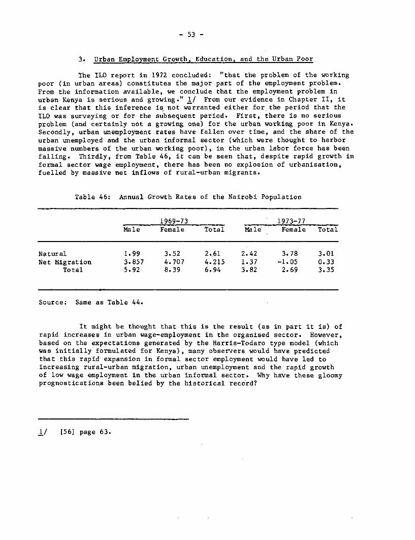
- 53 -

3. Urban Employment Growth, Education, and the Urban Poor

The ILO report in 1972 concluded: "that the problem of the workingpoor (in urban areas) constitutes the major part of the employment problem.From the information available, we conclude that the employment problem inurban Kenya is serious and growing." 1/ From our evidence in Chapter II, itis clear that this inference is not warranted either for, the period that theILO was surveying or for the subsequent period. First, there is no seriousproblem (and certainly not a growing one) for the urban working poor in Kenya.Secondly, urban unemployment rates have fallen over time, and the share of theurban unemployed and the urban informal sector (which were thought to harbormassive numbers of the urban working poor), in the urban labor force has beenfalling. Thirdly, from Table 46, it can be seen that, despite rapid growth informal sector wage employment, there has been no explosion of urbanisation,fuelled by massive net inflows of rural-urban migrants.

Table 46: Annual Growth Rates of the Nairobi Population

1969-73 1973-77Male Female Total Male Female Total

Natural 1.99 3.52 2.61 2.42 3.78 3.01Net Migration 3.857 4.707 4.215 1.37 -1.05 0.33

Total 5.92 8.39 6.94 3.82 2.69 3.35

Source: Same as Table 44.

It might be thought that this is the result (as in part it is) ofrapid increases in urban wage-employment in the organised sector. However,based on the expectations generated by the Harris-Todaro type model (whichwas initially formulated for Kenya), many observers would have predictedthat this rapid expansion in formal sector employment would have led toincreasing rural-urban migration, urban unemployment and the rapid growthof low wage employment in the urban informal sector. Why have these gloomyprognostications been belied by the historical record?

1/ [56] page 63.

- 54 -

It will be best to set out the implicit assumptions underlying theview that rapid urban formal sector employment growth would lead to risingrural-urban migration and urban unemployment and poverty. The basic assump-tion was that the urban formal sector wage was relatively rigid, and as notmuch faith could be put on rising rural incomes to narrow existing rural-urbanincome differentials, growth in formal sector urban wage employment would in-crease rural urban migration and the equilibrium level of unemployment, asmigrants equated their expected incomes from high wage urban employment withtheir rural incomes. In fact, between 1971 and 1977, the rural-urban incomedifferential declined substantially. Thus, real formal sector urban wagesfell by 22 percent during this period, whilst at least in Central Province,the per capita incomes of a substantial proportion (the top 60 percent) hadbeen growing at an annual rate of nearly 3 percent between 1963 and 1974. Ifthis trend also applied to the period 1971-77, then per capita smallholderincomes would have risen by 18 percent in this period. Hence, the rural-urban income differential is likely to have declined by about 34 percentbetween 1971 and 1977, as compared with its relative value in 1971.

Moreover, the Harris-Todaro type framework is known to be rathersimplistic in its assumptions about the homogeneity of the job-searchers, aswell as about the processes by which they adjust their expectations aboutfinding various types of high wage urban jobs. The so-called "bumping" modelof job search and urban labor market adjustment (see Fields [44]) provides amore subtle account of the workings of the urban labor market. Within thisframework, education is used as a screening device by potential employers,and hence it is important to examine the changing balances in the demand andsupply for different types of educated workers. Thus, if we can order jobsby the educational level that employers are currently using as a screen, themodel postulates that if someone with a higher level of education offershimself for a job which the employer has been filling with workers with alower-level of education, the more highly educated worker will be preferred.Hence job-searchers with levels of education that are higher than thosecurrent amongst workers at each rung in the job-ladder, will have a veryhigh probability of being hired. With an expansion of education relativeto the jobs at each rung in the job-ladder, the "excess" workers with therequisite education for that rung, will then find that it is increasinglyin their interest to offer themselves for jobs at the next lower rung inthe job ladder, because whereas their prospects of finding a job at the rungwhich was (till then) associated with their educational qualifications aredeclining, their prospects of finding jobs at the next lower rung stillremain high. As this realization sinks in, more and more of the "excess"workers at each rung of the job ladder and the accompanying educationalstatus, will offer themselves for jobs at lower and lower rungs of the jobladder. In the process, whilst employers will be seen to be upgrading thejobs at each rung in terms of the required educational qualifications, rela-tively more educated workers will be seen to be 'bumping' the less educatedcohorts off each rung of the ladder.

- 55 -

The resulting composition of the unemployed as well as the rateof unemployment over time will then be determined by three sets of inter-related factors. First, the relative imbalance between the jobs offeredand job seekers at each educationally differentiated rung in the job ladder,will determine how many people are in "excess" at that rung in the presentperiod. Next, of this 'excess', some will decide to remain unemployed, andtry their luck at the same rung in the ladder in the next period, and somewill lower their sights and seek and obtain (with near certainty) jobs atthe next lower rung in the ladder. This latter choice will be determinedin part by the speed with which job-seekers lower their expectations, whenexcess supply for a particular level of educated labor appears, as well astheir access to some means of financing the unemployment they might liketo choose whilst they are deciding whether or not to lower their sights.Thirdly, as the major source of financing is likely to be financial supportfrom relatives, and as (given the private costs), the more educated are likelyto belong to richer families, the relatively less educated are also likely tobe the least able to finance any prolonged period of unemployment, whilstthey are adjusting their job expectations. For these reasons we should expectthat, ceteris paribus, unemployment rates should be heavily biased towardsthe more educated, and that over time, with an expansion of education at eachlevel relative to the jobs, the bumping process will be forcing more and moreof the relatively less educated to choose between unemployment and continuedjob search. This should lead to a tendency for the unemployment rate to belowered over time. Both these predictions are borne out for Kenya by theevidence we have cited in Chapter II.

It remains for us to provide more direct evidence that in fact the'bumping' process which we have postulated accounts for these trends is infact taking place in urban Kenya. Table 33 provided evidence on the changingeducational profile of rural-urban migrants (the major component of urban job-seekers), which showed that their educational levels have been rising overtime. Secondly, Table 47 shows the falling propensity of secondary schoolleavers to migrate to the towns, between 1964 and 1976. Moreover, we havecomputed that the propensity to migrate of primary school leavers was .049between 1964-68 and .033 between 1969-76. Thus the propensity to migrateof secondary school leavers has fallen faster than that of primary schoolleavers.

- 56 -

Table 47: Migration Propensities of Form IV Leavers 1/'000

1964-68 1969-72 1973-76

National output of leavers 19.6 54.5 79.9Nairobi output of leavers 3.9 6.8 10.0

Non-Nairobi output of leavers 15.7 47.7 69.9Migrants with form IV Education 12.4 8.7 8.5

as of % of all migrants 23% 23% 34%Propensity of Non-Nairobi form IV

leavers to migrate to Nairobi .79 .183 .122

Mean Annual migration ('000) 3.1 2.9 2.8

1/ See (39a] Appendix 3 for derivation.

Finally, the table also shows the aggregate implications for the urban labormarket of these three processes, viz, a reduction in rural-urban incomedifferentials, 'bumping', and the changing expectations of job-seekers. Thenet migration stream of form IV leavers remained fairly constant over theyears, representing an increasing share of total migration but a reducedshare of total form IV output.

4. A Framework for Analysing Growth and Poverty-Redressal in Kenya

We are now in a position to provide a framework which shows theinterrelationships between growth (in particular in the urban sector) andpoverty redressal (mainly in the rural areas), which is based on the evidenceand analyses presented above, and within which various policy options can bediscussed. In order to bring out the novel features of this framework, itwill be best to contrast it with the implicit model of the interrelationshipsbetween urban growth and rural poverty redressal which seem to underlie thethinking of many observers of the Kenyan scene in the past.

Caricaturing somewhat, the conventional views on the likely conse-quences of Kenyan style development can be put as follows: Given existinginequalities in the distribution of assets (including human capital), andvarious structural rigidities which weaken intersectoral links, the promo-tion of rapid expansion of the private formal sector as well as of capitalistsmallholder farming, would lead to both increasing concentration in incomeand wealth in both rural and urban areas, but more seriously to the immiseri-sation of a growing non-formal urban labor force, as well as increasingproletarisation of the weakest groups in the rural countryside. In thisprocess, it is believed, the benefits of growth would not spread evenly or

- 57 -

fast enough amongst most sections of the population, because the adjustmentmechanisms in the form of price adjustments to particular sectoral imbalancesin demand and supply, would either be weak or absent. Hence, the structuralfeatures, for instance wage-differentials, would not be modified over thecourse of development, and instead maladjustments in demands and supplieswould show themselves up increasingly in the form of quantity adjustments.This led to predictions of increasing rural-urban migration flows into lowincome infor'mal sector employment or burgeoning unemployed pools of urbanlabor. Furthermore, in these implicit models, most of the flows of peopleand resources are assumed to be one way, from the rural to the urban sector.Many have therefore accepted the thesis that this type of development entailsa built-in urban bias, which needs to be corrected by deliberate acts ofpublic policy. The latter would be aimed at both changing the structure(for instance) of the existing income and asset distribution, as well as inreducing the one-way rural-urban flows. To the extent that various struc-tural features of the economy have to be accepted as given, these observerssee the promotion of the urban informal sector as the main panacea for urbanpoverty redressal. As regards the rural sector they see that: "for most ofthe rural.population, the problem is not the availability of jobs, in thesense of paid work for others, but the availability of land." 1/

Our thesis is that on the basis of the available evidence assembledand discussed above, many of the implicit assumptions underlying these viewshave proved to be false, and at the same time they are based on rather sim-plistic notions of the interactions between the rural and urban sectors inthe process of development. Thus one of the primary assumptions of the alter-native view that markets (and in particular labor markets) do not functionefficiently, with prices adjusting fairly smoothly to emerging imbalances indemand and supply is false. This is borne out by the very substantial realwage adjustments that have taken place, and the resulting failure of markedincreases in urban unemployment and low income wage-employment to emerge.Secondly, the reverse links between urban and rural areas, are at the least(in Kenya) just as important as the one way rural-urban links emphasized inthe past. What is more when account is taken of these two way flows, anyurban bias as exhibited for instance in a very rapid growth of urban formalsector employment, need not in any sense be at the expense of other groups(particularly those in the rural sector) in the economy. In fact a majorpart of our thesis is that it is the close two-way links between rural small-holders and formal sector employees, which in large part have determined thepace and extent of rural development in Kenya. Far from sucking in peopleand resources from the rural areas to the latter's detriment, the close rural-urban links that we have documented imply that the growth of the urban sectorhas shifted the production possiblity set of the rural sector. Finally, wehave provided some (admittedly speculative) evidence to suggest that it isprobably not the growth of capitqlist smallholder agriculture in Kenya which

1/ [56) page 23.

- 58 -

has led to the concentration of land, which in principle (and as we haveshown, in practice) by lowering the overall demand for rural labor, damagesthe interest of the rural poor. Instead, it is the growth of a particularclass of urban incomes (which we discuss in greater detail in the next chap-ter) which has boen mainly responsible for land concentration in Kenya. Thisremains the single most important structural source of the rural poverty prob-lem, as it leads to landlessness, outmigration to the drylands, and the emerg-ing conflict between these outmigrants and the pastoralists (all poor groups,by any standard in Kenya), for the meagre and diminishing land resources.

Finally, we have argued that, at least amongst smallholders thereis some evidence that, differences in land holding have not been the majordeterminant of household income and hence the incidence of poverty. It wasthe historically determined (relatively random) distribution of education,through its effects on the relative ability of different smallholder house-holds to obtain the urban-based off-farm income needed to finance smallholderinnovation, which was the prime determinant of differences in smallholderhousehold incomes. As household income and education are now increasinglycorrelated, the relatively benign distributional effects of the past dis-tribution of what has turned out to be a major asset viz. education, areless likely in the future.

We turn to an examination of the policy implications flowing fromthis framework of the two-way rural-urban interactions, for poverty redressalin Kenya. Before doing so, it may be useful to reiterate that in the type oftwo way rural-urban interactions charted in this chapter the notion of theeffects of growth "trickling down" is a very limited and highly misleadingrepresentation of the spread effects of growth. Thus, as we have shown,rural innovation has in no sense "trickled down" in Kenya; it is a directfunction of the growth of urban formal unskilled wage employment and itleads simultaneously to increases in income for most of the smallholdergroups (as it has been diffused across smallholder households irrespectiveof the size of farm), as well as of landless laborers.

- 59 -

IV. Policy Implications

Broadly speaking, we have identified three crucial processes whichproximately determine the incidence of poverty (which is mainly rural) inKenya. These are, first, the process of land concentration, which we haveargued is likely to have been fuelled by the increased demand for land forboth speculative and retirement purposes by the better educated and richerurban classes. Second, there is the process of smallholder innovation, whichwe have argued has been mainly determined by urban-based off-farm incomeobtained from the remittances of unskilled rural-urban migrants in the urbanformal sector. Thirdly, there is the increased competition for the meagreresources on marginal dry lands, between their traditional occupants (thepastoralists), and the landless outmigrants from areas of higher agriculturalpotential. The relevant policies must therefore be concerned with eitherhalting these processes (in the case of land concentration, and the competi-tion for marginal lands), or in promoting their further spread (in the caseof smallholder innovation). We, therefore, briefly discuss some relevantpolicy options under these three headings in this chapter.

1. Arresting Land Concentration

We can divide up the policy options into those concerning landconcentration amongst smallholders, and those concerning the problems of thelarge estates. We deal in this section, mainly with the smallholder problem,though in the last part we briefly discuss the issues relevant in formingjudgements on the appropriate policies towards the large farms.

We have argued that the increased concentration has most likelybeen due to the asset choices of high-income urban groups. We can influencethese choices through (a) direct intervention in the land market, (b) throughinterest rate policies, and the provision of alternative assets, and (c)through reducing the high urban incomes which finance this particular assetchoice. We examine policies under each of these sub-headings.

(a) Direct Intervention in the Land Market - Three forms ofdirect intervention in the land market may be considered. These are (i) aland tax; (ii) a capital gains tax on land; and (iii) legislative restric-tions on absentee ownership of land.

There are problems of administrative feasibility in the Kenyancontext, with both the first and last of these options.

Hence, a capital gains tax on land sales, may be the mostattractive option because to the extent land purchases are being fuelledby speculation in land values, such a tax will tend to reduce theexpected after-tax rate of return from such speculation. If the tax werelevied only on land bought and sold after the date of the institution of

- 60 -

the tax, the administrative costs would be lower as compared with a landtax, as the authorities would only have to monitor current and future salesof land. The tax would, therefore, only affect those who bought land witha view to speculating on its future resale value, and by reducing the returnto such speculation, it would reduce the speculative demand for land, whichwe have argued is likely to be a major source of land concentration. Afurther advantage of such a capital gains tax on land will be that to theextent it dampens the future rise in land prices, and thereby reduces theexpected rate of return on speculative current holdings of land, some ofthe latter might be put on the market, thereby reducing the current con-centration of land.

The major drawback of such a tax is that it provides an incen-tive for collusive evasion between buyers and sellers and the growth of so-called black money markets. This prospect is the likelier, the more thespeculative demand for land is fed by the rents accruing to certain sectionsof the urban population from various types of protective policies. If, how-ever, the proposed tax is combined with policies to reduce the generation ofthese urban rents (see below), then the dangers of such a tax leading to thegrowth of the black money market are likely to be reduced.

(b) Interest Rate Policy and Alternative Assets - To the extentthat the speculative demand for land is the result of the high expectedreturns to land as compared with alternative assets, raising the real rateof return on alternative assets, as well as the provision of newer high-yielding, and socially more productive assets for high income urban residents,would also tend to reduce the demand for land. It appears that the realreturn from savings deposits with banks or building societies have been low(see Table 48) and in recent years where interest rates have lagged behindchanges in the price level, are likely to have been negative. This effectsthe demand for land in two ways. First, the relatively low real return onalternative assets means that portfolio choices are biased towards holdingmore land. Secondly, as high income urban residents seem to be able toborrow at the existing low real interest rates to finance land purchases,they have a further incentive (as well as the means) to increase their landholdings.

Table 48: Real Interest Rates

Consumer Price Real Bank Savings Real Building SocietyYear Inflation Interest Rates Interest Rates

1974 33.9 -28.9 -27.91975 16.5 -11.5 -10.51976 8.4 - 3.5 - 1.2

Source: [10].

- 61 -

This suggests that raising interest rates on alternative assetsas well as on borrowing to finance land purchases will have some effect inreducing the asset demand for land.

(c) Urban Income Distribution - High income in the urban sectorcan be affected both through takation which reduces after tax incomes (whichfinance land concentration), as well as through measures which reduce highpre-tax incomes.

There is probably still some scope for raising direct taxes onthe higher urban income groups. However, the reduction in high pre-tax in-comes is likely to be a better way of tackling the problems of high urbanincomes. This is because a substantial part of these incomes are "rents"generated either through the operation of various protective foreign trade(and other public) policies, as well as those which accrue to the relativelyscarce "skills" of more educated labor. To the extent that public policy,in particular the high and uneven effective protection provided by the pro-tective foreign trade system, generates subsidies to the high-income non-wage urban sector (by implicitly taxing other groups in the country), areversal of these inefficient public policies would be highly desirable."Rents" accruing to high income wage-earners are the result of a continuingexcess demand for relatively more educated African labor. However, there isevidence that with the expansion in the supply of the educated labor force,these rents are likely to be eroded through the relatively efficient workingsof the Kenyan urban labor market. Thus, between 1963-74, the wage differen-tials between the mean of the top quarter of wage earners and the mean of theremaining three-quarters narrowed steadily. The differential was 7.1 in 1963,5.9 in 1969 and 4.2 in 1974. Also, within Nairobi, the proportion of wageearners receiving below half of the mean wage fell from 50 percent in 1972to 47 percent in 1976. Further evidence is provided in Table 49. This sug-gests that with the expansion of the educated labor force, and the resultingrelative wage adjustments in the urban labor market, the rents from bettereducation have, and are likely to continue to decline.

By contrast, as the protection regime was tightened in the early1970's we would infer that over time, the urban rents which in large partare financing increased land concentraton have come to be based primarilyon the monopoly profits generated by the protection regime rather than oneducation. A reduction in protection is, therefore, an important means forreducing the rents for high income urban residents, and thereby arrestingtheir demand for land.

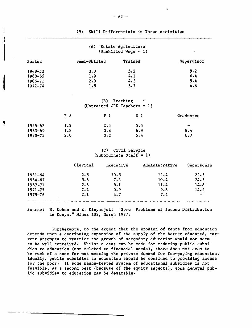
- 62 -

$9: Skill Differentials in Three Activities

(A) Estate Agriculture(Unskilled Wage - 1)

Period Semi-Skilled Trained Supervisor

1948-53 3.3 5.5 9.21960-65 1.9 4.1 6.41966-71 2.0 4.3 5.41972-74 1.8 3.7 4.6

(B) Teaching(Untrained CPE Teachers D 1)

P 3 P 1 S 1 Graduates

1955-62 1.2 2.5 5.51963-69 1.8 3.8 6.9 8.41970-75 2.0 3.2 5.4 6.7

(C) Civil Service(Subordinate Staff = 1)

Clerical Executive Administrative Superscale

1961-64 2.8 10.5 12.4 22.51964-67 3.6 7.5 10.4 24.51967-71 2.6 5.1 11.4 14.81971-75 2.4 5.9 9.8 14.21975-76 2.1 4.7 7.4 -

Source: M. Cohen and K. Kinyanjui: "Some Problems of Income Distributionin Kenya," Minus IDS, March 1977.

Furthermore, to the extent that the erosion of rents from educationdepends upon a continuing expansion of the supply of the better educated, cur-rent attempts to restrict the growth of secondary education would not seemto be well conceived. Whilst a case can be made for reducing public subsi-dies to education (not related to financial needs), there does not seem tobe much of a case for not meeting the private demand for fee-paying education.Ideally, public subsidies to education should be confined to providing accessfor the poor. If some means-tested system of educational subsidies is notfeasible,. as a second best (because of the equity aspects), some general pub-lic subsidies to education may be desirable.

- 63 -

(d) Policies Towards Large Farms - Large farms in Kenya are aure of farms owned by individuals, private and public companies, anderatives. They are also the refuge for a large but uncertain number

_ quatters. The undesirability of breaking up these large estates dependscruically upon the existence of economies of scale in the cash crop agricul-ture in which these farms specialise. The evidence on the existence and ex-tent of these economies of scale seems inconclusive at present. What doesseem odd is the legal prohibition on sales of land which would break upthese large estates. For, if the presumed economies of scale do exist, theywould be sufficient to provide private investors with an incentive to keepthe optimum sized large estates intact. There seems to be little reason whythis should be reinforced by any legal prohibition. Finally, to the extentthat some of these estates are held for speculative purposes, the proposedcapital gains tax on land sales would tend to reduce both the speculativegains from current holdings, as well as dampen future speculative demand.

2. Promoting Smallholder Innovation

We have argued that at present the major determinant of small-holder inovation is the easing of financial constraints through access tourban-based off-farm income earning opportunites. The policies for pro-moting smallholder innovation can therefore be classified into (a) thosewhich provide greater and more equal access to urban-based formal sectorjobs to the poorer smallholder rural-urban migrants, and (b) those whichprovide a supplement to the on-farm income flows, which by themselves areusually insufficient to finance smallholder innovation. We deal withpotential policies in both areas in this section.

(a) Access to Urban Formal Sector Jobs - The relative growthof formal sector jobs in Nairobi as compared with all other urban areas was5.1% versus 3.1% in the period 1967-76. This has meant that the CentralProvince smallholders have had much greater access to urban formal sectorjob opportunities, than those in Nyanza and Western Province. Thus in 1976,there were 254,000 formal urban sector wage-employees in Nairobi and CentralProvince, as compared with only 22,000 in Nyanza and Western Provinces. Fur-thermore, despite the fact that the smallholder population in Western andNyanza Provinces is twice that in Central Province, the increase in formalsector wage employment in Nairobi and Central Province between 1967-76 was76,000 as compared with only 6,000 in Nyanza and Western Province. Thissuggests that industrial location policy could have important effects inequalizing the regional distribution of urban formal sector job opportuni-ties.

To promote this regional dispersion of industry a regionallydifferentiated system of marginal employment allowances, a variant on asuggestion by A. Kervin could be considered. "Any corporation would beentitled to deduct from its taxable income a flat amount per additionalperson employed. For a new venture, it would work like an investmentallowance. The incentive given to investment would be the same, if itcarried average capital intensity. It would be higher if labor intensity

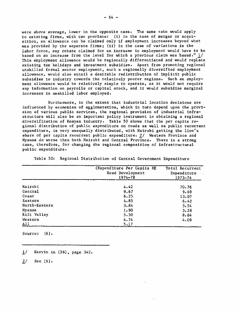
- 64 -

were above average, lower in the opposite case. The same rate would applyto existing firms, with two provisos: (i) in the case of merger or acqui-sition, an allowance can be claimed only if employment increases beyond whatwas provided by the separate firms; (ii) in the case of variations in thelabor force, any rebate claimed for an increase in employment would have to bebased on an increase from the level for which a previous claim was based." 1/This employment allowance would be regionally differentiated and would replaceexisting tax holidays and investment subsidies. Apart from promoting regionalunskilled formal sector employment, such a regionally diversified employmentallowance, would also entail a desirable redistribution of implicit publicsubsidies to industry towards the relatively poorer regions. Such an employ-ment allowance would be relatively simple to operate, as it would not requireany information on payrolls or capital stock, and it would subsidise marginalincreases in unskilled labor employed.

Furthermore, to the extent that industrial location decisions areinfluenced by economies of agglomeration, which in turn depend upon the provi-sion of various public services, the regional provision of industrial infra-structure will also be an important policy instrument in obtaining a regionaldiversification of Kenyan industry. Table 50 shows that the per capita re-gional distribution of public expenditure on roads as well as public recurrentexpenditure, is very unequally distributed, with Nairobi getting the lion'sshare of per capita recurrent public expenditure. 2/ Western Province andNyanza do worse than both Nairobi and Central Province. There is a strongcase, therefore, for changing the regional composition of infrastructuralpublic expenditure.

Table 50: Regional Distribution of Central Government Expenditure

(Expenditure Per Capita KE Total RecurrentRoad Development Expenditure

1974-78 1973-74

Nairobi 4.42 70.76Central 9.67 9.69Coast 6.25 13.07Eastern 4.85 6.42North-Eastern 3.84 3.54Nyanza 1.90 3.28Rift Valley 5.50 8.84Western 4.74 4.09All 5.17

Source: [6].

1/ Kervin in (56], page 342.

2/ See [6].

- 65 -

Whilst the above measures will to some extent equalize (andincrease) formal sector job opportunities across regions, there is still theproblem that the ability to seize these opportunities is likely to dependupon levels of education, and hence if access to these job opportunities isto be diversified, the distribution of education and opportunities will alsohave to be improved. This entails problems concerning both the access to, aswell as the quality of education currently available to the rural poor.

This is of some importance, for the processes whereby the effectsof urban growth were fairly rapidly transmitted to the Central Province small-holders, through the two way rural-urban interactions identified in Chapter 3,cannot be counted upon to work in the spread of the growth impulse in theother regions, without a diffusion of public education. Table 51 shows that,on a per capita basis, public expenditure on secondary education is low bothin absolute and relative terms in the poorer regions. At the least, theGovernment should consider raising the per capita development expenditure oneducation in the other regions to its current levels in Central Province.

Table 51: Development Expenditure on Secondary Education byProvince, 1974-78

Province Expenditure Per Capita (KE)

Nairobi 0.31Central 0.53Coast 0.25Eastern 0.20North-Eastern 0.20Nyanza 0.15Rift Valley 0.19Western 0.23All

Source: [6].

(b) Promoting Alternative Methods of Financing Innovation - Thoughwe have emphasized the importance of urban-based off-farm income as a majordeterminant of smallholder innovation, there are other ways in which thefinancial constraint on innovation (particularly amongst the poorer small-holders) could be eased. Though rural credit might seem to be the obviousway out, it appears that in Kenya there are good reasons, as noted in Chapter3, why both the ability and willingness to borrow are linked to the urban-based off-farm income flows of smallholder households. Therefore, thouglsome increase in financing smallholder innovation through increased ruralcredit may well be possible, we would not expect this to provide a majorsubstitute for urban-based off-farm income in the finance of innovation.

- 66 -

Another alternative would be to give cash grants for expenditureon innovation to the poorer smallholders. Besides the obvious administrativeproblems with such a policy, there is also the extra budgetary cost whichneeds to be taken into account. To minimize the latter, it maybe desirableto convert part of the current budget on extension services into cash grantsfor the poorer smallholders. It is likely that the current extension servicesare biased toward the richer farmers, whilst to the extent that the poorerfarmers cannot get access to funds to finance innovation, the availability ofextension services for them would seem to be irrelevant. It might, therefore,be worth using part of the extension budget to provide cash grants to thepoorer smallholders.

3. Policies for Alleviating Pastoralist Poverty

The various policy measures discussed in the previous two sectionsshould go some way towards alleviating the poverty of poor smallholders aswell as the landless, (of the latter through arresting concentration of landand hence the diminuition in demand for hired labor, and through more rapidsmallholder innovation and its associated increase in the demand for hiredlabor). This leaves the pastoralists as the final major poverty group forwhom we need to find some methods of poverty redressal. These policies areessentially concerned with both reducing the competition for the meagreresources of the pastoralist areas from landless outmigrants from the otherregions, as well as raising the productivity of the traditional occupationsof the pastoralists.

This implies that the first policy could be to-restrict the migra-tion of the landless from the other agricultural areas into the dry lands.Apart from reducing the pressure on the existing land resources in theseareas, this will also prevent the introduction of inapprorpiate farmingtechniques, which as we saw in Chapter 3, are increasingly leading to soilerosion, and hence a reduction in the cultivable area. As emphasized above,the problem of the landless will have to be solved by the policies which re-duce land concentration, promote smallholder innovation, and faster growthin urban wage employment. Their free outmigration to the drylands does notsolve their poverty problem, and worsens that of the pastoralists. Restric-tions of such migration would thus seem justified.

Two measures seem important for raising the current low levelsof income of pastoralists. These low levels are chiefly the result of over-grazing, which in turn is caused by the large and uneconomic size of theherds of the pastoralists. These over-large herds in turn reflect the lackof internalisation of the external diseconomies from overgrazing, what, ineffect, is public land, as well as the traditional asset preference of theMasai for cattle. The Government's policies to encourage the privatisationof land through group ranching are, therefore, wholly desirable in off-setting the current incentives to overgrazing. Furthermore, it appears thatthe traditional attitude towards holding cattle as an asset may be changing.Thus, traditionally the Masai have increased herd size at the onset of adrought, presumably in the hope that a larger total number of cattle would,

- 67 -

for any given proportion of the herd which was decimated by the drought, stillleave an absolutely larger number of post-drought cattle, than if the herdsize had not been increased. However, Campbell t8] found that, during themost recent drought, there seems to have been a generational split amongst theMasai in terms of recognizing the relative superiority of money as an asset.Thus Campbell reports that whereas nearly all the Masai below 35 years oldwere for reducing the herd size at the onset of the drought, the older Masaiwanted to follow exactly the reverse policy. It seems, therefore, that overtime the Masai will come to take a more 'modern' attitude towards the rela-tive merits of money and cattle as assets, and hence the traditional tendencytowards overstocking which has been uneconomic will be reversed.

Thus there are a number of policy options which could arrest themalign and aid the benign processes we have identified as being the majordeterminants of the extent of poverty redressal in Kenya in the recent past.

- 68 -

Appendix 1: Poverty Lines

Any income level which defines the criterion for "poverty" is essen-tially arbitrary. The purpose of such an exercise is not to reveal how manypeople are poor (almost all Kenyan smallholders are poor according to Westernusage of the word), but rather to be able to compare one rural group withanother group which is better off. We may then pose two revealing questions;why it is that some localities have a far higher incidence of poverty thanothers, and why, within a locality, some households have incomes very muchhigher than our poverty group. Thus the important attribute of a povertyincome line is that an adequate sample size should be retained on either sideof the line and a viable but significant poverty group identified for policypurposes. A rival approach to the concept of a poverty line is to identifysome minimum required standard of nutrition; the income level at which foodpurchases attain this standard serving as the povery line. Fortunately, inKenya the poverty lines suggested by these alternative approaches coincide.The household income level of 2,000 shillings per annum assigns 30% of thesmallholder population to poverty and is a class limit in IRS 1. It thusyields adequate sample sizes and does not pose data problems. Thorbecke,[90], adopts a nutritional approach and deduces a critical level of house-hold income of 2,050 s.p.a. at 1974 rural prices.

Applied to urban households, correcting for differences in pricelevels and household size, only a very small percentage of households werepoor. In order to make intra-urban comparisons it was therefore necessaryto use a much higher poverty line in order to get a reasonable sample size.This urban "poverty" line was set at roughtly twice the national poverty line(see [39a], Appendix 3).

- 69 -

Appendix 2: The Innovation Index

Innovation might involve a change in technology for a given productor a switch in the product mix. The former is measured by our data from IRS-Ion expenditure on farm inputs. The latter could be measured by area of land,number of crop units or crop yields. We were constrained by data availabilityto choose crop units (e.g. trees), but this is in any case probably the mostreliably measured survey data of the three possibilities.

Crop numbers data was limited to coffee trees, tea trees, cashewnuttrees, coconut trees, and numbers of livestock (improved or unimproved meas-ured in "livestock sampling units" (LSU) which were adjusted for age andtype of stock). One major omission among innovatory crops was hybrid maize;however, intensive studies of the adoption of hybrid maize have concludedthat the major constraint on further adoption is ecological rather than eco-nomic. Coconuts and cashews are non-existent outside Coast Province so wewere left with tea and coffee trees. Other omissions were pyrethrum (grownin Nyanza and Central but not Western or Coast) and cotton (grown only inNyanza and Western). Tea and coffee are common to Nyanza, Central and West-ern but not Coast. With livestock it was clear that only the possession ofimproved livestock could be regarded as an innovation. We therefore had thetask of building an innovation index as some composite of coffee trees, teatrees and improved livestock.

The IRS valued a LSU at 1,100 shillings. If we get an approximatevalue of mature coffee and tea trees by estimating their present value atfour times their annual income, then a coffee tree would be 115 shillings anda tea tree 15 shillings so that the weights assigned to the three componentsof the innovation index were tea tree = 1, coffee tree = 10, LSU = 74.

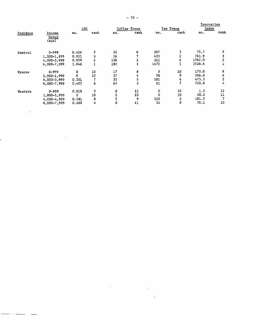
- 70 -

InnovationLSU Coffee Trees Tea Trees Index

Province Income no. rank no. rank no. rank no. rankGroup(spa)

Central 0-999 0.456 5 32 6 397 3 75.7 9

1,000-1,999 0.931 3 26 7 433 2 761.9 34,000-5,999 0.959 2 138 2 311 4 1762.0 26,000-7,999 1.846 1 192 1 1472 1 3528.6 1

Nyanza 0-999 0 10 17 8 0 10 170.0 81,000-1,999 0 10 37 4 26 9 396.0 64,000-5,999 0.301 7 35 5 101 6 473.3 56,000-7,999 0.403 6 63 3 61 7 720.8 4

Western 0-999 0.018 9 0 11 0 10 1.3 121,000-1,999 0 10 2 10 0 10 20.0 11

4,000-4,999 0.291 8 5 9 110 5 181.5 76,000-7,999 0.488 4 0 11 34 8 70.1 10

- 71 -

Bibliography

[1 ] Aldington, T., Wilson, F., Marketing of Beef in Kenya, IDS,Staff Paper 21.

[ 2 ] Aldington, T.J., Wilson, F.A., Some aspects of the Kenyan BeefEconomy, IDS, Discussion Paper 70.

3 ] Amsden, A.H., International Firms and Labor in Kenya 1945-70,London, 1971.

[ 4 ] Anderson, J.E., Report on the Conference of Harambee SchoolHeadmasters, IDS, Discussion Paper 95.

f 5 ] Berg-Schlosser, D., The Distribution of Income and Educationin Kenya, Munich, 1970.

[6 Bigsten, A., Regional Inequality and Development: A Case Studyof Kenya, National Economic Institute, Gothenburg, 1978.

[7 Bronensha, D., Mbere clans and land adjudication, IDS, StaffPaper 96.

[8 Campbell, D.J. Coping with Drought in Kenya Maasailand: Pastoralistsand Farmers of the Loitokitok area, Kajiado District, IDS,Nairobi, Working Paper 337, 1978.

[ 8a ] Crawford, E., and E. Thorbecke: "The Analysis of Food Poverty - AnIllustration from Kenya," Mimeo, 1979.

[9 ] Central Bureau of Statistics, Economic Survey, Annual, 1963-78,Nairobi.

[ 10 ] , Statistical Abstract, Annual, 1960-77, Nairobi.

[ 11 ] , Employment and Earnings, Annual, 1963-76, Nairobi.

[ 12 ] , Agricultural Census of Large Farm Areas, Annual,1954-71, Nairobi.

13 ] , Patterns of Income. Expenditure and Consumption ofAfricans in Nairobi in 1957-58, Nairobi.

[ 14 ] , African Agricultural Census 1960-61, Nairobi.

[ 15 ] , Patterns of Income. Expenditure and Consumptionof African middle class workers in Nairobi, 1963, Nairobi.

E 16 ] , Kenya Population Census, 1962, Nairobi.

17 ] , A Report on Economic Studies of Farming in NyanzaProvince, 1963, Nairobi.

- 72 -

18 ] Central Bureau of Statistics, Economic Survey of CentralProvince 1963/4, Nairobi.

19 ] , Economic Survey of Nyeri District of CentralProvince, 1964, Nairobi.

[ 20] , Survey of Services 1966, Nairobi.

[ 21 ] , A Comparison of the Intensity of Cultivation on Largeand Small Farms in Kenya, Statistical Digest, March 1972,Nairobi.

[ 22 ] , Estimates of the Income Elasticity of Demand forVarious Items in Nairobi, Mombasa and Kisumu,Statistical Digest, June 1972, Nairobi.

[ 23 ] , Population Prolection by District 1970-1980,Statistical Digest, June 1972, Nairobi.

[ 24 ] , Consumer Price Indices. Nairobi, March 1977, Nairobi.

[ 25 ] ,.Kenva Population Census 1969, Volumes I-IV, Nairobi.

[ 26 ] , Demographic Working Paper 3, Nairobi, 1976.

[ 27 ] , Demographic Working Paper 1, Nairobi, 1976.

[ 28 ] , Demographic Baseline Survey Report 1973, Nairobi.

29 ] , Preliminary Results of the Survey of Distribution,1971, Statistical Digest, June 1974, Nairobi.

[ 30 ] , Nairobi Household Budget Survey. 1974 (unpublished),computer results: Collier P. and Gunning J.W., Oxford,1978.

[ 31 ] - , Informal Urban Sector Employment, Annual, 1973-77,Nairobi.

[ 32] , Basic Food Prices in 80 Rural Markets, Nairobi.

[ 33 ] , Integrated Rural Survey 1, 1974-5, Nairobi, 1977.

[ 34 1 , Integrated Rural Survey 1, 1974-5, computer printouton income for Collier and Gunning, 1977, Nairobi.

[ 35 ] , Integrated Rural Survey 1, 1974-5, computer printouton consumption for G. Crawford, 1978, Nairobi.

[ 36 1 , National Demographic Survey, 1977 (unpublished)computer printout December 1978, Nairobi.

[ 37 ] __, Rural Household Survey Nyanza Province 1970/71 Nairobi.

- 73 -

38 ] Central Bureau of Statistics, Integrated Rural Survey II,1975-6, (unpublished) computer printout 1978, Nairobi.

39 ] Cowen, M. Notes on Capital, Class and Household Production,Department of Economics, Nairobi University, Mimeo.

39a ] Collier, P. and D. Lal: Poverty and Growth in Kenya, Mimeo, Studiesin Employment and Rural Development No. 55, IBRD, May 1979.

40 ] Cowen , M., Analysis of Nutrients in Food Consumption: Householdsin Magutu Location. Nyeri District 1971/72, Department ofEconomics, Nairobi University, mimeo, 1974.

[ 41 ] David, M.and Wyeth, P., Kenya Commercial Bank Loans in Rural Areas:a Survey, IDS Working Paper 342, Nairobi, August 1978.

[ 42 1 Department of Planning, Mathare Valley Survey, 1979, Nairobi..

[ 43 ] Elkan, W., Is a Proletariat Emerging in Nairobi? IDS Nairobi,Discussion Paper 168.

[ 44 ] Fields, G.S., "The Private Demand for Education in Relation toLabor Market Conditions in Less Developed Countries",Economic Journal, Volume 84.

[ 45 ] Gwyer, G., Trends in Kenya Agriculture in Relation to Employment,IDS Discussion Paper 153, Nairobi.

[ 46 ] Heyer, J., The Economics of Small-scale farming in lowlandMachakos, IDS Occasional Paper 1, Nairobi, 1967.

[ 47 1 Heyer, J.,Maitha J.K. and Senga W.m., Agricultural Development inKenya, OUP, Nairobi 1976.

48 ] Hunt, D.M., An Examination of the Distribution of Economic Statusand Opportunity in Mbere, Eastern Kenya, IDS Nairobi,Occasional Paper II, 1975.

[ 49 1 Hodd, M., "Income Distribution in Kenya 1963-72", Journal ofDevelopment Studies, Vol. 12 No. 3.

[ 50 ] House, W.J.and Rempel, H., "The Impact of Unionisation on NegotiatedWages in the Manufacturing Sector of Kenya", OxfordBulletin of Economics and Statistics, Vol. 38 No. 2.

[ 51 1 House, W.J. and Rempel, H., "The Impact of Unionisation on NegotiatedWages in the Manufacturing Sector in Kenya: a Reply",Oxford Bulletin of Economics and Statistics, Vol. 39 No. 3.

[ 52 ] House, W.J., and Rempel, H., "The Determinants of and changes in thestructure of wages and employment in the ManufacturingSector of the Kenyan economy, 1967-72", Journal ofDevelopment Economics, Vol. 3 No. 2.

- 74 -

[ 53 ] House, W.J. and Rempel, H., Kenya Employment Problem; an Analysisof the Formal Labor Market, O.U.P., Nairobi, 1978.

[ 54 1 House, W.J., The 1977 Nairobi Informal Sector Survey: SomePreliminary Results, Department of Economics, NairobiUniversity, mimeo 1978.

[ 55 ] Hunting, Hunting Report, Group Farm Rehabilitation Project.

[ 56 1 International Labor Office, Employment, Incomes and Equality.A Strategy for Increasing Productive Employment in Kenya,Geneva 1972.

[ 57 J Inukai, I. and Okello, J., Rural Enterprise Survey in NyeriDistrict Kenya. A report of the consultants to Danida,1971.

[ 58 ] Johnson, G.E.The Determination of Individual Hourly Earningsin Urban Kenya, IDS Discussion Paper 115, Nairobi,September 1971.

[ 59 ] Johnson,.G.E., Notes on Wages. Employment and Income Distributionin Kenya, Paper read at the Conference of York University,Nairobi 1971.

[ 60 1 Johnson, G.E. and Whitelaw, W.E., "Urban-Rural Income Transfers inKenya: An Estimated Remittances Function", EconomicDevelopment and Cultural Change, Volume 22 No.3.

f 61 ] Kilby, P. Preliminary Report on the Kenyan Informal Sector, IBRD,1979.

[ 62 ] King, A., The African Artisan, Nairobi, 1978.

[ 63 ] Kinyanjui, P.K., "Education, Training and Employment of SecondarySchool Leavers in Kenya", Education in Eastern Africa, 2(1) 1971.

[ 64 ] Kinyanjui, P.K. and Shepard, D., "Unemployment among SecondarySchool Leavers in Kenya", East Africa Journal, IX (8),1972.

[ 65 ] Kmietowicz, T. and Webley, P., "Statistical Analysis of IncomeDistribution in the Central Province of Kenya",Eastern Africa Economic Review, Vol. 7 No. 2.

[ 66 ] Leys, D., Underdevelopment in Kenya, London, 1975.

[ 66a I Lipton, M., Why Poor People Stay Poor, Temple Smith, London, 1977.

[ 67 J Liyingstone, I., Cowboys in Africa: The Socio-Economics ofRanching, IDS Occasional Paper 17, Nairobi.

- 75 -

68 ] Mbithi, P., Rural Sociology and Rural Development, EastAfrican Literature Bureau, Nairobi 1974.

[ 69 J Mbithi, P. Non-Farm Occupation and Farm Innovation, IDSStaff Paper 144, 1971.

[ 70 ] Mbithi, P. and Barnes, C., Spontaneous Settlement Problem in Kenya,East African Literature Bureau, 1975.

[ 71 J Migot-Adholla, S.E.Migration and Rural Differentiation in Kenya,PhD, UCLA, 1977.

[ 72 J Matingu, M.N., Rural-to-Rural Migration and Employment, M.A.Thesis, Department of Sociology, Nairobi University, 1974..

[ 73 ] Ministry of Economic Planning and Development, Development.Plan,1974-78.

[ 74 ] Ministry of Education, Annual Report, 1975, Nairobi.

[ 75 2 Ministry of Labor, Annual Report, 1974, Nairobi.

[76 ] Ministry of Labor, Labor Turnover Survey, 1972, Nairobi.

[77 ] Momanyi, J.O.B. Socio-Economic Change in Gusiiland, B.A. Thesis,Nairobi Univrsity, Department of Sociology, 1976..

78 ] Morrison, C. Income Distribution in Kenya, (mimeo), IB,D, 1973.

[79 ] Musyoki, R.N., Socio-Economic Status of Families and 4ocialParticipation: A Multi-Dimensional Analysis of Commitmentand Alienation in Rural Kenya, M.A. Thesis, Departmentof Sociology, Nairobi University.

( 80 ] Nairobi City Council, Annual Report, 1974, Nairobi.

C 81 ] Njoroge, R.W., Some Factors Influencing Performance in ElarambeeSecondary Schools, M.A. Thesis, Department of Sociology,Nairobi University 1977.

[ 82 ] Nyangira, N., Relative Modernisation and Public Resource Allocationin Kenya, East African Lieterature Bureau, Nairobi, 1975.

C 83 ] Posner, R. Preliminary results of a survey of the labor force onmixed farms in Trans-Nzoia, IDS Discussion Paper 57.

[ 84 ] Rempel, H., Harris, J., and Todaro, M., Rural-Urban LaborMigration a Tabulation of Responses to the Questionnaireused in the Migration Survey, IDS Discussion Paper 92.Nairobi.

- 76 -

[ 85 Rempel, H., Labor Migration into Urban Centres and UrbanUnemployment in Kenya, Ph.D , Department of Economics,University of Wisconsin, 1970.

[ 85a ] Rempel, H, and R.A. Lobdell: "The Role of Urban-to-RuralRemittances in Rural Development," Journal of DevelopmentStudies, April 1978.

[ 86 ] Richardson, H.W., Khanna, A. and Sampaio, O.A., NationalUrban Development Strategy, IBRD 1977.

[ 87 ] Sandbrook, R., Proletarians and African Capitalism: the Kenyan Case,1960-72, Cambridge, 1975.

[ 88 ] Scott, M.F.G. McArthur, J., and Newbery, D., Project Appraisal inPractice: The Little-Mirrlees Method Applied in Kenya,London, 1976.

[ 89 ] Thias, H.H. and Carnoy, M., Cost-Benefit Analysis in Education:a Case Study of Kenya, IBRD 1972.

[ 90 ] Thorbecke, E. and Crawford, E., Employment, Income Distribution,Poverty Alleviation and Basic Needs in Kenya, ILO 1978.

[ 91 ] Weeks, J., Employment growth in Kenyan manufacturing: anotherlook at labor absorption, Birkbeck College, DiscussionPaper in Economics No. 21, London 1974.

[ 92 ] Westley, S.B., Johnston B.F. and David, Martin, Summary reportof a workshop on a food and Nutrition Strategy forKenya, IDS Occasional Paper 14, 1975.

[ 93 ] Wilson, R.J.A., Land Control in Kenya's Smallholder FarmAreas, IDS Staff Paper 89, Nairobi 1971.

[ 94 ] Wilson, R.J.A., Economic Implications of Land Registration inKenya's smallholder areas, IDS Staff Paper 91,Nairobi 1971.

[ 95 ] Whitelaw, Nairobi Household Survey: Description of the Methodologyand Guide to the Data, IDS Discussion Paper 116,Nairobi 1971.

[ 96 1 World Bank, Kenya-Into the Second Decade (John Hopkins, 1975).