-r=AIAA-2002-0840

Drag Prediction for the DLR-F4 Wing/Bodyusing OVERFLOWand CFL3D on an Overset Mesh

J. C. VassbergPhantom WorksThe Boeing CompanyLong Beach, CA 90807,USA

P. G. BuningConfigurationAerodynamicsNASA Langley ResearchCenterHampton, VA 23681, USA

C. L. RumseyComputational Modelingand SimulationNASALangley ResearchCenterHampton, VA 23681, USA

40th AIAA AerospaceSciences Meeting& Exhibit14-17January,2002 / Reno, NV

I II II

For permission to copy or republish, contact the American Institute of Aeronautics and Astronautics

1801 Alexander Bell Drive, Suite 500, Reston, Va, 22091

https://ntrs.nasa.gov/search.jsp?R=20030005441 2019-02-16T20:32:16+00:00Z

Drag Prediction for the DLR-F4 Wing/Body

using OVERFLOW and CFL3D on an Overset Mesh

John C. Vassberg *Phantom Works

The Boeing Company

Long Beach, CA 90807, USA

Pieter G. Buning _

Configuration Aerodynamics

NASA Langley Research Center

Hampton, VA 23681, USA

Christopher L. Rumsey t

Comp. Modeling and Simulation

NASA Langley Research Center

Hampton, VA 23681, USA

14 - 17 January, 2002

Abstract

This paper reviews the importance of numerical drag

prediction in an aircraft design environment. Achronicle of collaborations between the authors and

colleagues is discussed. This retrospective provides

a road-map which illustrates some of the actions

taken in the past seven years in pursuit of accu-

rate drag prediction. The advances made possible

through these collaborations have changed the man-

ner in which business is conducted during the designof all-new aircraft.

The subject of this study is the DLR-F4

wing/body transonic model. Specifically, the workconducted herein was in support of the I ot CFD Drag

Prediction Workshop, which was held in conjunction

with the 19 th Applied Aerodynamics Conference in

Anaheim, CA during June, 2001.

Comprehensive sets of OVERFLOW simulations

were independently performed by several users on

a variety of computational platforms. CFL3D was

used on a limited basis for additional comparison on

the same overset mesh. Drag polars based on thisdatabase were constructed with a CFD-to-Test cor-

rection applied and compared with test data from

three facilities. These comparisons show that the

predicted drag polars fall inside the scatter band of

the test data, at least for pre-buffet conditions. This

places the corrected drag levels within 1% of the

averaged experimental values. At the design point,

the OVERFLOW and CFL3D drag predictions are

within 1-2% of each other. In addition, drag-rise

characteristics and a boundary of drag-divergenceMach number are presented.

"AIAA Associate Fellow, DPW Organizing Committee,Boeing Technical Fellow

tAIAA Associate Fellow, Research ScientistAIAA Associate Fellow, Research Scientist

Copyright 1_)2002 by Vassberg, Bunlng _ Rumsey.Published by the AIAA with permission.

Nomenclature

b 2

AR Wing Aspect Ratio - sr,sa Acoustic Speedb Wing Span

C_ Drag Coefficient =qo¢ Srel

CL Lift Coefficient =q_ Sref

C_I Wing Reference Chordcount Drag Coefficient Unit = 0.0001

D DragDPW Drag Prediction Workshop

e Oswald's Efficiency FactorL Lift

M Mach Number

RANS Reynolds-Averaged Navier-StokesRan Reynolds number - _ v_ cry!

_-oo

S_] Wing Reference AreaSFC Specific Fuel Consumption

W WeightY+ Wall Distance =

_w

q Dynamic Pressure -- ½PV2c_ Angle of Attack

A¢/4 Wing Quarter-Chord Sweepec Signifies Freestream Conditions

1 Introduction

In reflection, as the 100-year anniversary of flight

draws near, it is truly amazing just how far the in-

dustry has progressed. This rapid advance in the

science, technology, and business of flight was madepossible through a blend of competition and coop-

eration between industry rivals, government agen-cies, and academic institutions around the world. It

is in this spirit that the Drag Prediction Workshop

(DPW) was conducted [1]-[2]. Participants from six

nations came together for a common goal - to assess

the state-of-the-art of drag prediction using Compu-

tational Fluid Dynamics (CFD) methods based on

the Reynolds-Averaged Navier-Stokes (RANS) equa-tions.

Vassberg, Buning _'¢Rumsey, AIAA Paper 2002-08_0, Reno, NV 1 o] 23

Why is drag prediction so important to the indus-

try of flight? In short, drag represents the irrecov-

erable aerodynamic losses associated with a flight-

based mission. For example, consider the generic

task of delivering a payload between distant city

pairs. The Breguet-Range equation, which aptly ap-

plies to long-range missions of jet aircraft, is:

MLRange- D SFC \ _/o J" (1)

Here, M is the cruise Mach number, L & D are the

aerodynamic forces of lift and drag, respectively, a

is the acoustic speed, SFC is the specific fuel con-

sumption of the engines, W0 is the aircraft landing

weight, and Wj is the weight of fuel burned duringthe flight. The Breguet-Range equation illustrates

the importance of drag prediction as a function of

lift and Mach number in the context of aerodynamic

design; it also provides a glimpse into the interplay

between the various disciplines.

Referring to Eqn (1), one might assume that the

aerodynamic efficiency of an aircraft is represented

by --_, the propulsion efficiency is embedded in

SFC, and that the structural efficiency directly im-

pacts I470. Interestingly, historical trends of in-

service transport aircraft indicate that very little im-

provement in the _ metric has been accomplishedin the past 50 years. Yet it would be somewhat

naive to state that no aerodynamic advances have

been made during this period. In actuality, improve-

ments in aerodynamics have better served aircraft

designs by trading them for improvements in other

disciplines. For example, the ability to increase the

thickness-to-chord ratio of a wing while maintain-

ing -_ not only reduces the structural weight of

the wing, it also provides additional fuel volume.

In terms of Eqn (1), an aerodynamic improvementof this nature would manifest itself as a decrease in

W0 and an increase in W! with the net result being

an increase in range. Reducing the aircraft's empty

weight has the added benefit of reducing the cost ofthe vehicle. Obviously, this aerodynamic improve-

ment would not be apparent in the trend charts ofML

D "

Assume that an airline would like to provide a ser-

vice between two cities with an aircraft that, when

fully loaded with payload and fuel, is 1% short on

range. Since the aircraft is fuel-volume limited, the

only recourse is to reduce the payload weight. In

relative terms, a typical ratio of weights might have

21470 and Wpa_to_ 1Wf = g = g W0. In this scenario,Eqn (1) shows that the operator would have to re-

duce the payload (read revenue) by 7.6% to recoverthe 1% shortfall on range. Since most airlines op-

erate on very small margins, this service most likely

will no longer be a profit-generating venture. This

example illustrates that in the current business of

flight, a 1% delta in aircraft performance is a sig-nificant change. While improving an aircraft's per-

formance by 1% may not be a trivial task given the

usual constraints, losing 5% is easily done if attention

is not paid to detail (e.g., juncture flows, external

doublers, gaps, etc.).

Now consider a more typical case where the air-

craft does not suffer from a shortfall on range. In

round numbers, the Direct Operating Costs (DOC)

of a transport aircraft can be itemized as: 50% for

the cost of ownership, 20% for fuel burn, 20% for

crew salaries and maintanence, and 10% for miscel-

laneous other items. From an airline's perspective, if

the DOC of its fleet of aircraft could be reduced by

5% with a new design (while providing the same set

of services to its customers), the airline would mostlikely retire its entire fleet and replace it with the

new aircraft [3].

So how can aerodynamics be leveraged to im-

prove the economics associated with a flight-basedmission? A simplified high-lift-system design that

retains _ and CL m_ reduces manufacturing andmaintanence costs as well as part count. Increas-

ing the cruise Mach number without reducing MLD

reduces the time-dependent costs such as crew and

maintanence. And the classic, increasing --%-gwith-out penalizing the other disciplines reduces fuel burn.

These are just a few examples of how aerodynamic

advances can have an impact on DOC... and all of

these require accurate drag predictions.

To push aerodynamic technologies forward, it is

becoming more important that accurate drag predic-tion become a consistent product of the CFD com-

munity. Once this prerequisite is accomplished, thefull benefits of automated aerodynamic shape opti-

mization may begin to be realized.

With the various on-going design programs, theseare exciting times for the aircraft industry. A prime

example is the Blended-Wing-Body (BWB) whichhas established a renaissance in the design of a family

of all-new aircraft [4]. This revolutionary concept is

enabling aerodynamic advances in all of the aboveareas, and then some. It presents challenges, yet

offers significant opportunities, and as a result, a 5%

reduction in DOC is within grasp. Suffice it to say

that aerodynamics is not a sunset technology, but

rather, it is as important today as it was a century

ago; only the stakes have changed.

2 Background

The first and second authors embarked on a collab-

orative effort which began in late 1994. Specifically,

this study was to determine what was required to

Vassberg, Buning _ Rumsey, AIAA Paper 2002-08_0, Reno, NV 2 o] 23

obtain accurate drag results from the OVERFLOW

code [5]. At that time, a typical simulation for a

commercial transport configuration yielded a drag

error of about 100 counts, where the total drag of

the aircraft was nominally 300 counts. Results for

the High-Speed Research (HSR) platforms were evenworse; computed drag values were occasionally neg-

ative. Clearly, that state-of-the-art was quite unac-

ceptable. In fact, there were prominent members of

the aerodynamics community at large who felt that

accurate drag predictions from RANS-based CFD

methods might never be accomplished. Nonetheless,

a systematic study of gridding guidelines proved to

be the key, and by mid 1995 the errors in computed

absolute drag values for pre-buffet cruise conditions

approached the 1-3% level. This collaboration, along

with the NASA Advanced Subsonic Transport (AST)

Program cooperative work with (then) McDonnell

Douglas Aerospace-West [6], was the catalyst for the

development of the 7-zone grid system for wing/body

configurations with the signature collar grid at the

wing/body juncture. These gridding guidelines wereused as the basis for the DPW baseline grids, and will

be discussed later in the paper. However, the end re-

sult was that the size of a grid suitable for accuratedrag prediction was nominally 4-5 times larger than

that previously used. In addition, the number of iter-

ations required for convergence on drag rather than

pressures also jumped by a factor of 2-5, depending

on the case. Hence, the cost of OVERFLOW sim-

ulations for drag prediction increased by more than

an order-of-magnitude relative to those used for the

calculation of pressure distributions.

In another collaborative effort which began inearly 1995, the first two authors agreed that a paral-

lel version of OVERFLOW for distributed process-

ing was in order. The original parallel code was

based on the Parallel Virtual Machine (PVM), and

more recently, has been ported to use the Message-

Passing Interface (MPI) [7]. For more than five

years, the Aerodynamic Design group in Long Beach,

CA has almost exclusively used a parallel version of

OVERFLOW on distributed clusters for production

overset-grid CFD simulations. A parallel-processing

capability such as this was necessary for accurateCFD drag predictions t.o be economically feasible

in an aircraft design environment [8]. Turn-around

time was further improved with the addition of gridsequencing and full multigrid to accelerate solution

convergence [9].

The combination of the above two collaborations

had an immediate impact on the B717-200 design

(previously called the MD-95). Here, several aerody-

namic fairing designs for various juncture flows were

evaluated using OVERFLOW. In all cases, the pre-dicted drag increments were later confirmed to be

extremely accurate in wind-tunnel tests [10]. In one

particular case, a pocket of separated flow was identi-

fied in the numerical simulations just prior to a wind-

tunnel entry. This prompted a flow-visualization

run that confirmed the separation. Before the test

was over, a fillet for this troublesome region was de-

signed, fabricated with stereolithography, shipped tothe wind tunnel, and tested.

In 1996, the first author invited a team of NASA

personnel from the Ames and Langley Research Cen-

ters to participate in the aerodynamic design of the

MD-XX trijet aircraft. The NASA group worked on-

site and fully integrated within the MD-XX team.

Due to the successes of CFD drag prediction on the

MD-95 program, the MD-XX Design Office elevated

the role and importance of CFD in the design envi-

ronment. They did so by scheduling the freeze of the

final loft lines of the cruise geometry several months

prior to the first wind-tunnel test entry which wouldverify the aircraft's aerodynamic performance. Al-

though this program was later cancelled, it marked

a dramatic change in the manner in which business is

conducted in the design of an all-new aircraft. This

philosophy lives on today in advanced programs such

as the Blended-Wing-Body [4], [11].The lessons learned in the above efforts have been

augmented with subsequent studies on drag pre-

diction conducted under various programs and ex-

tended to other CFD methods such as CFL3D [12],

SYN107 [13]-[14], and TLNS3D [15]. Within BoeingPhantom Works Long Beach, OVERFLOW remains

tile work-horse for complex transport configurations,

CFL3D is heavily used on the BWB and re-entry ve-

hicle programs, while SYN107 and TLNS3D round

out the tool chest by providing aerodynamic shapeoptimization capabilities.

Since 1995, while the errors in predicted absolute

drag have stablized, the complexity of the configura-

tions being analyzed has consistently increased. To-

day, the size of an overset grid system for a complete

B747-400 configuration (comprised of a cruise wing,fuselage, pylons, flow-through bifurcated fan and

core cowls, winglets, vertical and horizontal tail com-

ponents) is approximately 20 million nodes. Further-

more, these simulations are being performed with the

aircraft trimmed to specified center-of-gravity loca-tions. After correcting for excrescences, internal cowl

drags, etc., comparisons with flight test data haveconfirmed that the numerically predicted absolute

drag values are within the band of uncertainties.

The next challenge for drag prediction is to im-prove the level of accuracy for post-buffet cruise con-

ditions as well as for high-lift configurations. Im-

proved high-lift drag prediction may become criti-

cal to achieve the pending more-stringent environ-

mental requirements on take-off and landing noise.

Vassberg, Buning _ Rurnsey, AIAA Paper 2002-0840, Reno, NV 3 o/ 23

Unfortunately, current state-of-the-art RANS-based

CFD methods cannot consistently predict accurate

pressures for these flows. Until this is accomplished,

there is little hope that accurate drag values will be

attained here as well. An accomplishment of this

magnitude will likely be possible only through thecumulative work of many collaborative efforts suchas those aforementioned.

The works noted above were conducted by a mul-

titude of individuals, including the authors, under

numerous collaborations between Boeing Phantom

Works Long Beach and the NASA Ames and Lan-

gley Research Centers. A subset of those who were

involved are: Dan Bencze, Bob Biedron, Dick Camp-

bell, William Chan, Roger Clark, Susan Cliff, Mark

DeHaan, Lie-Mine Gea, Robb Gregg, James Hager,

Ray Hicks, Rick Hooker, Dennis Jespersen, SteveKrist, Steve Mysko, Bob Narducci, Mike Olsen, Rick

Potter, Stuart Rogers, Dino Roman, Tony Sclafani,

Jeff Slotnick, Richard Wahls, and Mark Whitlock.

3 DLR-F4 Geometry

The case chosen for the DPW is the DLR-F4

wing/body configuration [16]. Several factors wereconsidered in the decision to use this geometry as

the test-bed for the workshop. One factor was the

availability of test data from multiple wind-tunnel

facilities. Another was that this configuration is rep-

resentative of current transonic transport aircraft.

The general layout of the DLR-F4 is provided in

Figure 1. This configuration is typical of a transonic

aircraft designed to cruise at M = 0.75. The wing

quarter-chord is swept 25 ° with a leading-edge sweep

of 27.1 ° and an outboard trailing-edge sweep of 18.9 °.The 9.5 aspect-ratio wing is rigged with a dihedral

angle of 4.8 °. Its planform is void of a leading-edge

glove, yet includes a yehudi which extends to 40%

semispan, completely unsweeping the trailing edge

of the inboard wing. This planform is representa-tive of wings that accommodate retractable main

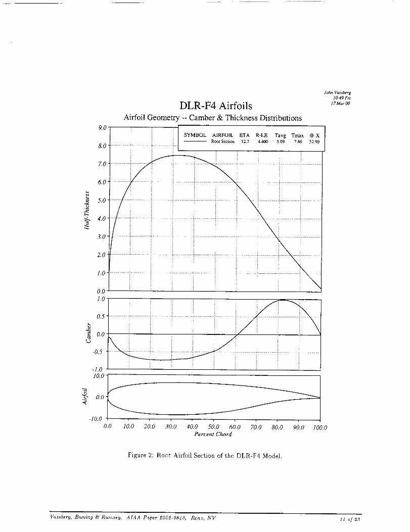
landing gear. The airfoil sections are supercriticalwith thickness-to-chord ratios of 14.9% at the side-

of-body, reducing to 12.2% outboard. The wing trail-

ing edge has a blunt base of 0.5% local chord. Fig-ures 2-3 provide the thickness and camber distribu-

tions, as well as the geometry, for the root and out-

board airfoil sections, respectively. The wind-tunnel

model has a wing semispan of 585.7mm, a mean

aerodynamic chord of 141.2rnm, a reference area of145,400rnm 2, and reference center at x = 504.9mm.

The fuselage length is 1,192turn. Its constant bar-rel section has a diameter of 148.42rnrn, which be-

gins at x = 250ram and extends to x = 626rnm.

No special fillets are incorporated at the wing-body

juncture, yielding a sharp corner everywhere on the

intersection line. The DPW geometry also includesthe aeroelastic twist of the wind-tunnel model under

a loading which corresponds to the nominal cruise

condition of M = 0.75 and CL = 0.5, with a dy-

namic pressure of q = 43,434Pa.

4 DPW Overset Grid

The overset mesh generated for the DPW was based

on the original process developed in 1995. The grid

is comprised of 7 zones, 4 of which conform to the

geometry and three box grids that transition the sys-

tem to the farfield boundary. The 4 conforming gridsdefine the volumes next to the fuselage, the wing-

body juncture, the wing, and the wingtip. Two in-

termediate boxes surround the fuselage and wing ge-

ometries, while the remaining farfield box extends

outward about 150 reference-chord lengths.

For this exercise, the surface grids were con-

structed using Gridgen-V13 [17] and are depicted

in Figure 4. These surface grids were then ex-

truded outward using HYPGEN [18] to generate the

4 surface-abutting volume grids. Figure 5 shows a

close-up of the wingtip grid. Figures 6-7 illustratethe collar grid at the wing-body juncture.

The hole-cutting and fringe-point coupling steps

were performed manually using GMAN [19]. The

overlap and blanking of the meshes near the wing's

mid-chord are shown in Figure 8.

On the wing surface, the chordwise spacing at both

the leading and trailing edges is approximately 0.1%local chord. The trailing-edge base is defined with 5

evenly-spaced points. The wake is represented with

65 points in the streamwise direction. The spanwise

spacing is about 1% semispan at the root and 0.1%

at the tip. On the fuselage nose and after-body, the

maximum grid spacing is nominally 5mm. In thedirection normal to the viscous surfaces, the first-

layer spacing is about 0.001rnrn, which correspondsto Y+ __ 1. Also in this direction, the maximum

growth rate of the grid spacing is 1.24. Figure 9

provides an itemization of the individual grid di-mensions, surface points, total grid points, and non-

blanked real points. The complete grid system is

comprised of 3,231,377 real points, with 54,445 re-

siding on the viscous surfaces.

The guidelines used to generate the DPW overset

mesh purposely omitted two gridding rules; these will

be discussed now for completeness. The first is re-

lated to the manner in which OVERFLOW computesskin-friction drag. For this calculation to be second-

order accurate, the first two layers of the grid nor-

mal to viscous walls must be evenly spaced. While

this rule was not strictly enforced, the spacing ra-

Vassberg, Buning _ Rumseg, AIAA Paper 2002-0840, Reno, NV _ o] 23

tios of the first two layers were fairly close to unity.The second rule is related to the grid resolution at a

blunt trailing-edge base. Here, it is the first author's

standard practice to include a trailing-edge cap grid

that wraps around the blunt base in a C-clamp fash-

ion. This grid normally has half of the cells on the

base and the remaining cells evenly split between the

upper and lower surfaces. It normally extends about

5-10% upstream of the trailing edge. However, in the

case of the DLR-F4 wing where the gradients near

the trailing edge are relatively benign, inclusion of a

high-resolution cap grid is probably not required for

accurate drag prediction.

One final note. After the DPW was held, the

Long Beach Aerodynamic Design group has finallytransitioned from GMAN to PEGASUS-V5 [20] to

provide semi-automatic hole-cutting and fringe-point

coupling capabilities. There were several reasons

for this lag, most were related to drag prediction.

With that being said, the current parallel version of

PEGASUS-V5 has proved to be a very useful tool,and one now appropriate for drag prediction. Fur-

ther, it will continue to improve through the on-going

collaborations within the PEGASUS community.

5 Wind-Tunnel Test Data

The DLR-F4 model was tested in three European

facilities: NLR-HST, ONERA-S2MA, and DRA-8xS.

The repeatability of these facilities was on the order

of +5 counts. While the AGARD AR-303 report [16]

presented this data, an unfortunate element of this

documentation was that the drag coefficients were

only tabulated to three decimal places. Hence, the

archived public-domain data has an effective scatterband of +10 counts.

In an attempt to alleviate the uncertainty in-troduced by the truncation, the first author post-

processed the public-domain data with two filters.

The first data enhancement augmented the drag co-efficients with the coefficients of axial and normal

forces. This process reduced the uncertainty of the

tabulated values from the original 5 counts, down

to as small as 0.8 counts, depending on the case.

The second data enhancement was a careful digiti-

zation of the drag polar figure in the AGARD re-

port. This digitization was also checked to be consis-

tent with the reduced uncertainty bands derived by

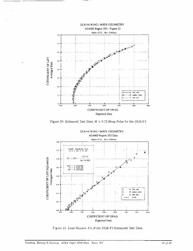
the first enhancement process. The resulting wind-

tunnel drag polars are provided in Figure 10. A more

detailed explanation of these filters can be found in

the Data Enhancement presentation on the DPW

website [1].The enhanced wind-tunnel test data for M = 0.75

has been collapsed to a curve, by fitting a limited

range of the data to an equation of the followingform.

= co0 + (2)7r ,e, AR'

Here, Coo and e are the free coefficients of the curve

fit and the aspect ratio of the DLR-F4 wing is AR =

9.437262. Including data from all three tests, but

limited to the lifting range of

0.2 ___cL < 0.55, (3)

a least-squares curve fit yields CDo = 0.018388 and

e = 0.829146. Eqn (2) now becomes:

cICo = 0.018388 + 24.5825_-------5' (4)

and is applicable for the CL range given in Eqn (3).

The curve fit given by Eqn (4) and associated test

data are provided in Figure 11.Since Case 1 of the DPW exercise is to compute

the drag at M = 0.75, Ren = 3M, and CL = 0.5, it

might be of interest to apply Eqn (4) to this condi-tion, which yields:

0.5 _Co = 0.018388+ -- - 0.02856. (5)

24.58255

The drag polars presented in the next section usethe enhanced wind-tunnel data, rather than data

taken directly from the AGARD AR-303 report.

6 Results

Included in this section are comprehensive sets of

OVERFLOW solutions which were performed on theDPW baseline overset mesh. Also included is a lim-

ited set of data generated by CFL3D on the sameoverset mesh for additional comparison. A more

complete set of CFL3D solutions for the DPW base-

line 1-to-1 multiblock mesh is documented by the

third author in Reference [21].

For the DPW exercise, the authors purposely did

not coordinate with each other in an attempt to

obtain independent results on the DLR-F4 config-

uration. In spite of this, the first two authors ranOVERFLOW with essentially the same set of critical

input parameters. Both used central difference scalardissipation with the Spalart-Allmaras (SA) turbu-

lence model. However, slightly different versions of

OVERFLOW were run, different computer platforms

were utilized at different levels of precision, and dif-

ferent methods to converge on lift were employed. It

is good to report that these differences yielded no no-

ticeable variations in the computed forces, moments

or pressures.The first author ran full convergence on all so-

lutions, starting each solution from a uniform flow

Vassberg, Buning gJ Rumsey, AIAA Paper 200_-0840, Reno, NV 5 o/23

at freestream conditions. Full multigrid accelerationwas used with 150 iterations in both the coarse and

intermediate meshes, and 3,000 iterations in the fine

mesh. All solutions were run by specifying an angle-

of-attack, even when a specific lifting condition was

desired. All computations were performed using 64-

bit precision. Version 1.8m was run in parallel usingMPI on a cluster of 6 Hewlett-Packard C3610 work-

stations, each with 2 GB of RAM, and connectedwith a switched 100BaseT ethernet. Each solution

required about 13 hours of wMl-clock time. Alpha

sweeps were conducted at 10 Mach numbers, thenthese data were interpolated on CL to derive the re-

quired alphas for CLs of 0.3, 0.4, 0.5, and 0.6. In all,

a total of 53 OVERFLOW solutions were performed

to obtain drag polars at the 10 Mach numbers. To

define the drag-rise curves, the drag polars were in-

terpolated on CL2 to obtain the corresponding C9values.

The second author and colleagues ran some cases

with a fixed angle-of-attack and some with a specified

lift-coefficient. All computations were performed us-

ing 32-bit precision. Version 1.8s was run in parallel

on three different computer platforms, an SGI Oc-

tane with 2 processors, an SGI Origin using 8 proces-

sors, and a cluster of 6 Compaq XP-1000 machines.

Wall-clock timings for these systems were 18.5 hours,

7.5 hours, and 6 hours per 1,000 fine-mesh iterations,

respectively.

For a limited set of conditions on the overset mesh,

the third author ran CFL3D with 3_d-order upwind

differencing with Roe flux difference splitting and us-

ing the SA model. These solutions were converged

4,800 multigrid iterations on the fine grid only, and

were run by specifying an angle-of-attack. A non-

dedicated SGI Origin was used with one processor,

requiring approximately 270 hours of wall-clock timeper solution.

Figures 12-13 illustrate the OVERFLOW conver-

gence histories of lift and drag, respectively, for a

freestream condition of M = 0.75, Ren = 3M, and

c_ = -1 °, which yields CL = 0.409 and CD = 263.3

counts. These forces have essentially converged by2,000 iterations on the fine mesh. Note the scale

on these figures; lift increments are 0.002 and dragincrements are a count.

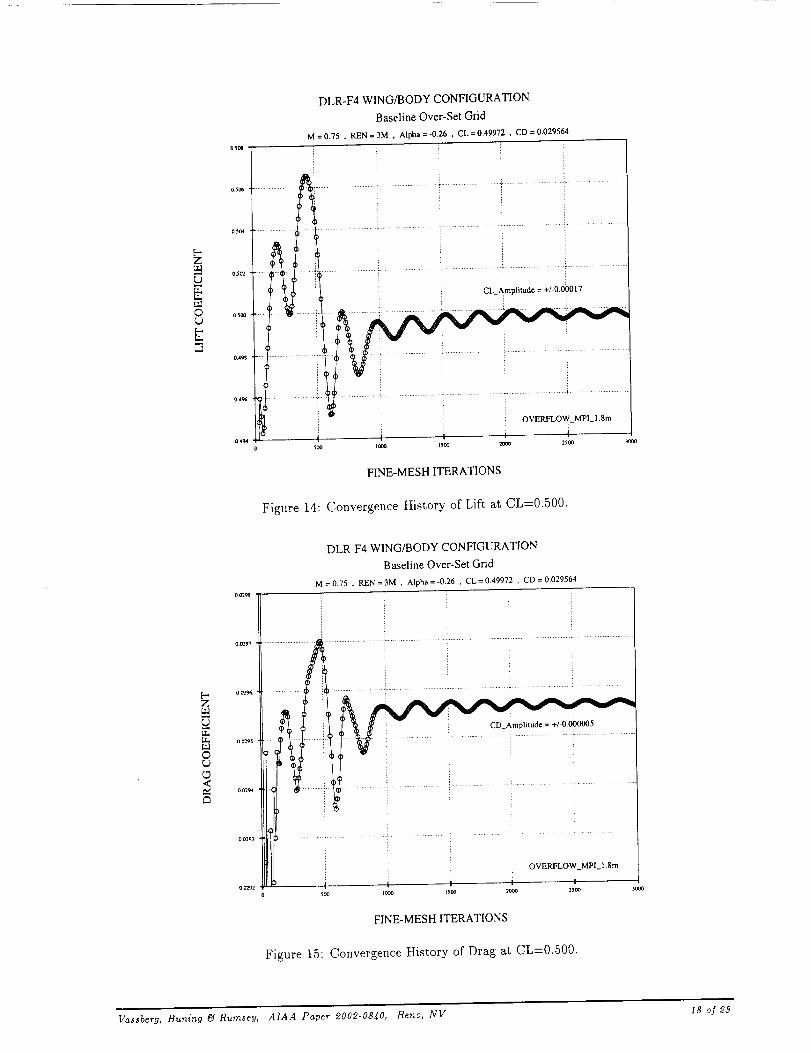
Figures 14-15 provide a similar set of OVER-

FLOW convergence histories, however, these corre-

spond to the cruise lifting condition of CL = 0.5

with corresponding Co = 295.6 counts. Unlike the

previous condition, these forces continue to oscillate

through all 3,000 iterations, albeit at very small am-

plitudes. The cause of these fluctuations is a small

pocket of separated flow that appears near the trail-

ing edge of the wing-body intersection; see Figure 16.

Figure 17 provides a comparison of pressure distri-

butions between OVERFLOW and test data at the

cruise design point of M = 0.75 and CL = 0.5. Note

that the leading-edge peaks are missed because of

the difference in alphas between the numerical sim-

ulation and the tests. Also, the isobars in this figurehint to the small pocket of flow separation on the

upper-surface near the root trailing edge.

An important aspect of comparing results fromOVERFLOW and CFL3D on the overset mesh is to

estimate variation due to choice of CFD code. Fig-

ure 18 shows a comparison of pressure distributionsat M = 0.75 and a = 0 °. At this a-matched con-

dition, results are very close and computed leading-

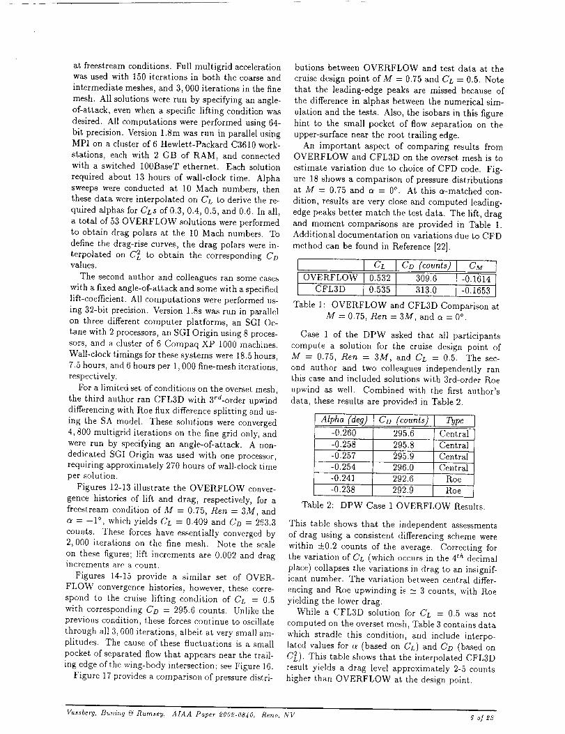
edge peaks better match the test data. The lift, drag

and moment comparisons are provided in Table 1.Additional documentation on variations due to CFD

method can be found in Reference [22].

I cL IcD(co.nts)l CMOVERFLOW 0.532 309.6 I -0.1614

CFLaD 0.535 313.0 I -0.1653

Table 1: OVERFLOW and CFL3D Comparison at

M=0.75, Ren=3M, anda=0 °,

Case 1 of the DPW asked that all participants

compute a solution for the cruise design point ofM = 0.75, Ren = 3M, and CL = 0.5. The sec-

ond author and two colleagues independently ranthis case and included solutions with 3rd-order Roe

upwind as well. Combined with the first author's

data, these results are provided in Table 2.

Alpha (deg) CD (counts) Type

-0.260 295.6 Central

-0.258 295.8 Central

-0.257 295.9 Central

-0.254 296.0 Central

-0.241 292.6 Roe

-0.238 292.9 Roe

Table 2: DPW Case 1 OVERFLOW Results.

This table shows that the independent assessments

of drag using a consistent differencing scheme were

within +0.2 counts of the average. Correcting for

the variation of CL (which occurs in the 4 th decimal

place) collapses the variations in drag to an insignif-icant number. The variation between central differ-

encing and Roe upwinding is __ 3 counts, with Roe

yielding the lower drag.While a CFL3D solution for CL = 0.5 was not

computed on the overset mesh, Table 3 contains data

which stradle this condition, and include interpo-

lated values for _ (based on CL) and Co (based on

C2). This table shows that the interpolated CFL3D

result yields a drag level approximately 2-5 counts

higher than OVERFLOW at the design point.

Vassberg, Buning _4Rumsey, AIAA Paper 2002-0840, Reno, NV 6 o] 23

Alpha (aeg) Co (eo. ts) I CL-1.000 266.0 0.416

-0.294 298.0 0.500

0.000 313.0 0.535

Table 3: CFL3D Results.

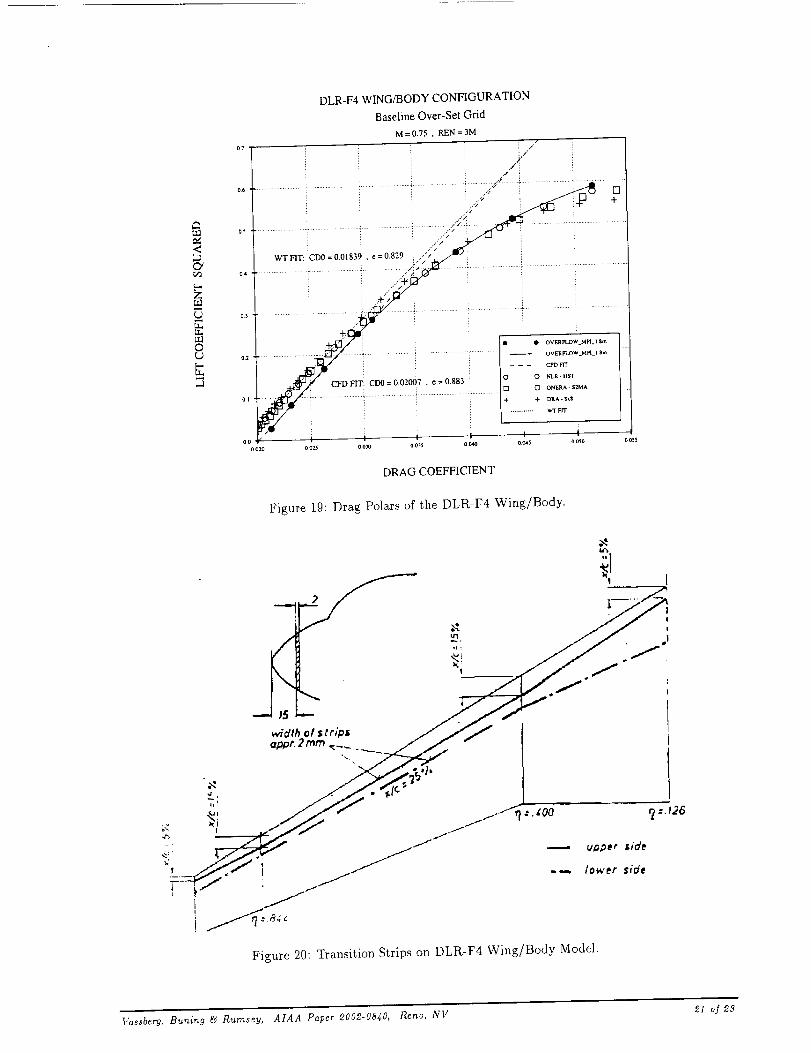
Figure 19 provides the OVERFLOW computed

drag polar for M = 0.75 and includes the wind-

tunnel data for reference. The data in this figure areinconsistent in that the numerical simulations were

performed assuming fully-turbulent flow, while thetests allowed laminar runs of 5-15% chord on the

wing's upper surface and 25% chord on the wing's

lower surface. Figure 20 shows the transitions pat-tern used in the tests.

To assess the impact on drag caused by this dif-

ference, FLO22 [23]-[24] was used to generate dragpolars of fully-turbulent flows and flows tripped with

the pattern of Figure 20. These results are shown

in Figure 21. Also shown in this figure are least-

squares curve fits of the polars. When differenced,

these curve fits yield a shift in drag of

CD _mtt = 13.7-- 2.3. C_L counts. (6)

= 13.7- 2.3.0.5 2

= 13.1 counts. (7)

Applying the correction of Eqn (6) to the fully-

turbulent OVERFLOW and CFL3D results yields

the drag polars depicted in Figure 22. Once the effect

of transition is taken into consideration, the numer-

ically predicted results lie within the scatter of the

experimental data.

If the cruise point is reviewed, the drag predictionswith the correction of Eqn (7) become:

CD over]tow corrected "_- 0.02825,

CD cfl3d-v6 .... ected _- 0.02849. (8)

Comparing Eqns (8) with Eqn (5) shows only a 1%

difference in drag levels between CFD and experi-ment.

During the DPW, Schwamborn and Sutcliffe pre-

sented a result using the DLR-TAU code which also

addressed this CFD-to-Test difference. Their presen-

tation is available on the DPW website [1]. On page

5, the data labeled Case 3 and Transition indicate

that at CL = 0.5, the correction is:

C,) hijt(0.5) 12 counts. (9)

Eqns (7) & (9) are very consistent with each other

and are independent estimates of the effects on drag

of the laminar runs vs. fully-turbulent flows.

Figure 23 illustrates the drag-rise curves as pre-dicted by the OVERFLOW solutions. From bottom-

to-top, the four curves of this figure correspond toCL = 0.3, 0.4, 0.5, and 0.6, respectively. Also in-

cluded in this figure is a cross-plot curve, depicted by

the dotted line, which illustrates the drag-divergenceMach number for the DLR-F4. The definition of

Mdd is taken to occur when the drag-rise slope is

dCD/dM = 0.05. Using these results, the drag-

divergence boundary is determined and is shown in

Figure 24.

The above definition of Mdd is motivated par-

tially by the Breguet-Range Eqn (1), and by eco-

nomic forces (related to block times) that push the

operating Mach number upward towards the 99%

Long-Range-Cruise (LRC) point. From Figure 24, itappears that the DLR-F4 wing is capable of cruis-

ing in excess of M = 0.775 at the lifting condi-

tion of CL = 0.5. However, these estimates have

all been made at a wind-tunnel Reynolds number,

rather than at flight.

7 Conclusions

The importance of drag prediction within an aircraft

design environment is reviewed. A seven-year ret-rospective of collaborations is given which illustrates

some of the steps taken by the authors and colleagues

in pursuit of accurate drag predictions. The suc-

cesses of this body of work have had a significant

impact on the manner in which Ml-new aircraft de-

signs are approached.

The DLR-F4 wing/body configuration has been

analyzed by OVERFLOW and CFL3D using an over-set mesh. This study focused on the prediction of

drag as a function of lift and Mach number for awind-tunnel Reynolds number of 3M based on ref-

erence chord. For pre-buffet conditions, results pre-

sented herein show that the numerical drag predic-

tions are within 1% of the averaged wind-tunnel

data, and the OVERFLOW and CFL3D drag pre-dictions are within 1-2% of each other. This level of

uncertainty is comparable to that of the wind-tunneldata itself.

Comprehensive sets of OVERFLOW simulationswere independently performed by several users, on

a variety of computational platforms. These solu-

tions spanned 10 Mach numbers from 0.5 to 0.82.

By coincidence, most of these solutions used cen-

tral differencing, scalar dissipation and the Spalart-

Allmaras turbulence model. However, a variety of

parallel computational platforms were used, a mix-

ture of single and double precision simulations were

performed, and slightly different versions of OVER-

FLOW were applied. It is good to say that the vari-

Vassberg, Bunln 9 F_4 Rurnsey, AIAA Paper 2002-08g0, Reno, NV 7 of 23

ation of these results are negligible. In addition, a

few computations were performed with Roe upwind-

ing. The difference in drag levels between the two

differencing stencils is on the order of 1%.The Drag Prediction Workshop called for the CFD [3]

calculations to be performed fully turbulent. The

available wind-tunnel data, however, was tripped at

5-15% on the wing upper surface and 25% on thelower surface. Corrections for the CFD-to-Test dif-

ferences were estimated using FLO22, running semi- [4]complete polars for both flows. The study derived a

correction of about 13 counts at the design point.

This is comparable to a similar and independent

study based on the DLR-TAU code. Drag polarsbased on OVERFLOW were constructed with the [5]

CFD-to-Test corrections and compared with wind-

tunnel test data. These comparisons show that the

predicted polars fall within the scatter band of the

test data, at least for pre-buffet conditions.

Four drag-rise curves were constructed from theOVERFLOW solutions. Using a slope definition for [6]

drag-divergence Mach number, the Mde boundary

for the DLR-F4 wing/body was constructed.In future workshops, a grid-resolution study

should be included by providing a series of

parametrically-consistent meshes of varying resolu-

tion. Post-processing the results from such a se-

quence using Richardson extrapolation will provide

further insight into the resolution required for a de-

sired level of accuracy, at least for the c_se being [7]

investigated.

Acknowledgment

The authors acknowledge The Boeing Company and [8]The National Aeronautics and Space Administration

for their support in the Drag Prediction Workshop,and for providing a working environment that not

only allows, but encourages the numerous collabo-rative studies that have and will continue to occurbetween the two institutions. [9]

The second and third authors would like to ac-

knowledge S. Melissa Rivers, Joseph H. Morrison,

and Robert T. Biedron of the NASA Langley Re-

search Center, for their contributions to the authors' [10]respective Drag Prediction Workshop presentations.

References [11]

[1] AIAA CFD Drag Prediction Workshop Website.http://www.aiaa.org/tc/apa/dragpredworkshop

/dpw.html, June 2001.

[2] D. W. Levy, J. C. Vassberg, R. A. Wahls,

T. Ziekuhr, S. Agrawal, S. Pirzadeh, and M. J.

[12]

Hemsch. Summary of data from the first AIAA

CFD Drag Prediction Workshop. AIAA pa-

per 2002-08_I, Reno, NV, January 2002.

J. C. Vassberg and R. D. Gregg. Overview ofaerodynamic design for transport aircraft. Pre-

sentation, First M.I.T. Conference on Compu-

tational Fluid and Solid Mechanics, Cambridge,

MA, June 2001.

R. H. Liebeck. Design of the Blended-Wing-

Body subsonic transport. Wright Brothers Lec-

ture, AIAA paper 2002-0002, Reno, NV, Jan-

uary 2002.

P. G. Buning, D. C. Jespersen, T. H. Pulliam,

G. H. Klopfer, W. M. Chan, J. P. Slotnick, S. E.

Krist, and K. J. Renze. OVERFLOW User'sManual, Version 1.8L. Technical report, NASA,

July 1999.

L. M. Gea, N. D. Halsey, G. A. Intemann,

and P. G. Buning. Applications of the 3-D

Navier-Stokes code OVERFLOW for analyz-

ing propulsion-airframe integration related is-

sues on subsonic transports. In Proceedings of

19th Congress of the International Council of

the Aeronautical Sciences (ICAS 94), number

ICAS-94-3.7.4, pages 2420-2435, Anaheim, CA,

September 1994.

D. C. Jespersen. Parallelism and OVER-

FLOW. NA$ Technical Report NAS-98-013,

NASA Ames Research Center, October 1998.

http://www.nas.nasa.gov/Research/Reports

/Teehreports/1998/PDF/nas-98-013.pdf.

J. Conlon. OVERFLOW code empowers Com-

putational Fluid Dynamics. InSights Issue 5,

NASA High-Performance Computing and Com-

munications Program, Moffett Field, CA, April1998.

D. C. Jespersen, T. H. Pulliam, and P. G. Bun-

ing. Recent enhancements to OVERFLOW.

AIAA paper 97-06_, AIAA 35th Aerospace Sci-

ences Meeting, Reno, NV, January 1997.

J. C. Vassberg. CFD-Based Design. Presenta-

tion, Stanford University, Palo Alto, CA, Febru-

ary 2000. Graduate Seminar Series.

D. L. Roman, J. B. Allen, and R. H. Liebeck.

Aerodynamic design challenges of the Blended-

Wing-Body subsonic transport. AIAA pa-

per 2000-4335, Denver, CO, August 2000.

S. L. Krist, R. T. Biedron, and C. L. Rum-

sey. CFL3D User's Manual. NASA-TM 1998-

208444, NASA, June 1998. Version 5.0.

Vassberg, Buning _J Rurnseg, AIAA Paper 200_-0840, Reno, NV 8 o/23

[13]A. JamesonandJ.C.Vassberg.Computationalfluiddynamicsfor aerodynamicdesign:Itscur-rentandfutureimpact.AIAA paper 2001-0538,Reno, NV, January 2001.

[14] J. C. Vassberg and A. Jameson. Aerodynamic

shape optimization of a Reno race plane. Int'l

Journal of Vehicle Design, 28(4):318-338, 2002.

Special Issue on: Design Sensitivity and Opti-mization.

[15] G. Kuruvilla, R. P. Narducci, and S. Agrawal.

Development and application of TLNS3D-

Adjoint: A practical tool for aerodynamic shape

optimization. AIAA paper 2001-2400, Anaheim,CA, June 2001.

[16] G. Redeker. DLR-F4 wing-body configuration.

In A Selection of Experimental Test Cases for

the Validation of CFD Codes, number AR-303,

pages B4.1-B4.21. AGARD, August 1994.

[17] Gridgen user manual version 13. Technical re-

port, Pointwise, 1998.

[18] W. M. Chan, I. T. Chiu, and P. G. Buning.

User's manual for the HYPGEN hyperbolic grid

generator and the HGUI graphical user inter-face. NASA-TM 108791, NASA, October 1993.

[19] T. D. Gatzke, W. F. LaBozzetta, G. P. Frin-frock, J. A. Johnson, and W. W. Romer.

MACGS: A zonal grid generation system for

complex aero-propulsion configurations. AIAAPaper 91-2156, June 1991.

[20] N. E. Shus, W. E. Dietz, S. M. Nash, M. D.

Baker, and S. E. Rogers. PEGASUS user's

manual version 5.1c. Technical report, MICROCRAFT, July 2000.

[21] C. L. Rumsey and R. T. Biedron. Compu-

tation of flow over a drag prediction work-

shop wing/body transport configuration usingCFL3D. NASA-TM 2001-211262, NASA, De-cember 2001.

[22] C. L. Rumsey, D. O. Allison, R. T. Biedron,

P. G. Buning, T. G. Gainer, J. H. Morrison,S. M. Rivers, S. J. Mysko, and D. P. Witkowski.

CFD sensitivity analysis of a modern civil trans-port near buffet-onset conditions. NASA-TM

2001-211263, NASA, December 2001.

[23] A. Jameson. Transonic potential flow calcula-

tions using conservative form. In Proceedings of

AIAA 2nd Computational Fluid Dynamics Con-ference, pages 148-161, June 1975.

[24] P. A. Henne and R. M. Hicks. Wing analysis

using a transonic potential flow computational

method. NASA-TM 78_6_, July 1978.

Vassber9, Buning _ Rumsey, AIAA Paper 200_-0840, Reno, NV 9 of 23

3Figure 1: General Layout of the DLR-F4 Model.

Vassberg, Buning _, Rumsey, AIAA Paper 2002-08_0, Reno, NV I0 oJ 23

DLR-F4 Airfoils

Airfoil Geometry -- Camber & Thickness Distributions

SYMBOL AIRFOIL ETA R-LE Tavg Tmax @ XRoot Section 12.7 4.400 5.09 7.46 32.90

John Vassberg

10.'49 Fri

17 Mar O0

g:

1.0

0.5"

_o

.- 0.0

-0.5

-1.0

10.0

0.0

-10.0

0.0 10.0

J

20.0 30.0 40.0 50.0 60.0 70.0 80.0 90.0 100.0

Percent Chord

Figure 2: Root Airfoil Section of the DLR-F4 Model.

Vassber9, Buning _ Rurnsey, AIAA Paper 2002-08_0, Reno, NV 1l of 23

5

DLR-F4 Airfoils

Airfoil Geometry -- Camber & Thickness Distributions

SYMBOL AIRFOIL ETA R-LE Tavg Tmax @ XOutboard Sections 100.0 1.005 4.10 6.09 37.17

2.0 _ : _ ! i i i '

i ! i i i i 'J.5 ...............i..............i...............i...............!...............i...............i.....................

"_1.o ............i..............i...............i...............i...............i ........

0.5

0.0

0.0 10.0 20.0 30.0 40.0 50.0 60.0 70.0 80.0 90.0 100.0Percent Chord

John Vassberg10.'50 Fri

17 Mar O0

Figure 3: Outboard Airfoil Section of the DLR-F4 Model.

Vassberg, Buning _ Rumsey, AIAA Paper _002-08g0, Reno, NV 12 of 23

Figure 4: Four Grids Defining the Wing/Body/Wake Surfaces

Figure 5: Wing-Tip Grid

Vassber9, Bunin9 #l Rumsey, AIAA Paper _00,_.08,_0, fteno, NV 13 o] 23

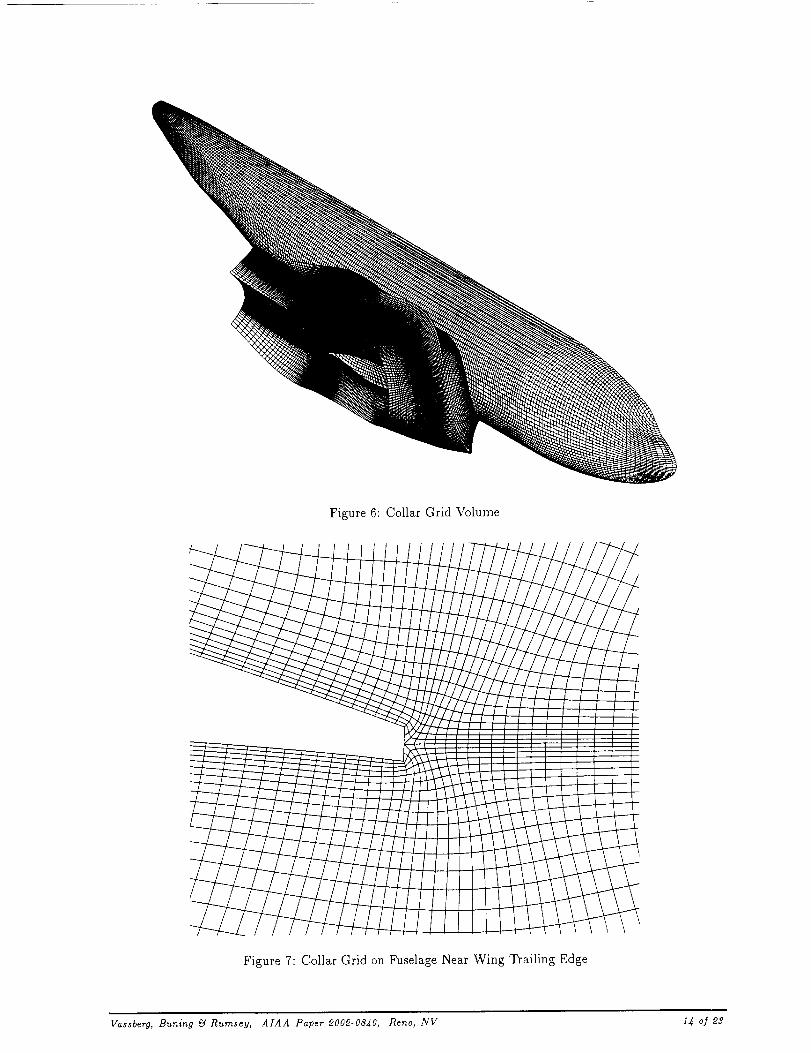
Figure 6: Collar Grid Volume

Figure 7: Collar Grid on Fuselage Near Wing Trailing Edge

Vassberg, Bunin9 _ Rurnsey, AIAA Paper _00_-08,_0, Reno, NV 14 of 23

V ......_- i_._=;_

Figure 8: Field Grids Near Wing Mid-Chord Location

Total viscous-surface points: 54445

Total grid points: 3727462

Total non-blanked grid points: 3231377

Grid points across the TE base 5

Farfield boundary is a box _150 chord lengths away.

grid id jd kd surfpts gridpts %pts1 49 273 49 13377 655473 17.6

2 385 65 49 22209 1226225 32.9

3 385 62 49 15934 1169630 31.4

4 25 141 49 2925 172725 4.6

5 121 22 43 0 114466 3.1

6 67 74 46 0 228068 6.1

7 75 39 55 0 160875 4.3

Totals : 54445 3727462

realpts %real562499 17 4

1092327 33 8

1038606 32 1

135219 4 2

76840 2 4

168408 5 2

157468 4 9

3231377

description

fuselagecollar

wing

wingtipfuse_box

wing_box

global_box

Figure 9: Statistics of the DPW Baseline Overset Grid.

Vassberg, Buning _ Rumsey, AIAA Paper 2002-08_0, Reno, NV 15 o] 23

-..1[..u©b.,Zt.Ll

t-UU.]©(..)

_1_ 04

>o< o_

DLR-F4 WING / BODY GEOMETRY

AGARD Report 303 - Figure 12

Mach = 0.75 , Re = 3 Million

E

! i ! ....I-

o i i ..+...... !i i i .* ..... i i

.................... i...................... _........... ,,,,::_ .................. ;......... ! ...........i * ....

...................... i...... _ ..... !............................ ............................ {......................... i.......................

............................... ........i i i

°°0 015 0o20 0025 0030 0035 0.040 0o45

COEFFICIENT OF DRAG

Digitized Data

Figure 10: Enhanced Test Data M = 0.75 Drag Polar for the DLR-F4.

e¢<

[..Z

U:Z

©

<

DLR-F4 WING / BODY GEOMETRY

AGARD Report 303 Data

Math = 0.75 , Re = 3 Million

Least Squares Fit

CL**2

o_o CD = CD0 + .......... D

cDo: o.o183B8 _ Xo2_ .... e = 0.829146 ............... i ........... o/_ : ..... ...........

AR = 9.437262

o

o_o ..................................................... .......o, ....... i........ ...................

! o °

. o o o .LR -.s-r

: o i [] o Or_R^.mMAo,o o_ o o .......

oo_ ........ _ ................. .....onC_oDo. i i

0 015 0 020 0 022 0024 0026 0028 0030 00_2 0034

COEFFICIENT OF DRAG

Digitized Data

Figure 11: Lea.st-Squares Fit of the DLR-F4 Enhanced Test Data.

Vassberg, Bunin9 _ Rumse_/, AIAA Paper 200_-0840, Reno, NV 16 o] 28

Z

©

,..a

DLR-F4 WING/BODY CONFIGURATION

Baseline Over-Set Grid

M = 0.75 , PEN = 3M , Alpha = -1.00 , CL = 0.40864 , CD = 0.026332

i

a...a ..................................................................................................................

5OO 1oo0 1500 I'ao0 25OO

FINE-MESH ITERATIONS

Figure 12: Convergence History of Lift at CL=0.409.

Z

rT

_L 00_6_

©

DLR-F4 WING/BODY CONFIGURATION

Baseline Over-Set Grid

M = 0.75 , REN = 3M , Alpha = -I.00 , CL = 0.40864 , CD = 0.026332

FINE-MESH ITERATIONS

Figure 13: Convergence History of Drag at CL=0,409.

Vassberg, Bunin9 U Rumsey, AIAA Paper 200_-0840, Reno, NV I7 of _3

Z

©

,..1

OJC2

DLR-F4 WING/BODY CONFIGURATION

Baseline Over-Set Grid

M --- 0.75 , REN = 3M , Alpha = -0.26 , CL = 0.49972 , CD = 0.029564

(

a

_t

.................... ÷.......................................................................... :.................

i_ i

.......,.............................................................................................................................r _ m

............................ i.,

CL_Amplitude = +/-0.00017

5oo lootl 15oo 2o0o 25oo

FINE-MESH ITERATIONS

Figure 14: Convergence History of Lift at CL=0.500.

Z

©

<

0 0796

0_95

O.O294

DLR-F4 WING/BODY CONFIGURATION

Baseline Over-Set Grid

M -- 0.75 , PEN = 3M , Alpha = -0.26 , CL = 0.49972 , CD --. 0.029564

z

i i i i

OVERFLOW MPI 1 .Smi! f

50_ too0 i_oo ?OO0 25tao

FINE-MESH ITERATIONS

Figure 15: Convergence History of Drag at CL=0.500.

Vassber9, Buning g3 Rumsey, AIAA Paper 2002-08_0, Reno, NV 18 of 23

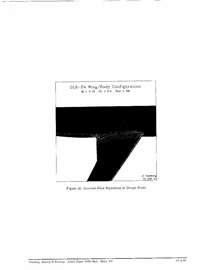
DLR-F4 Wing/Body ConfigurationM = 0.75 , CL = 0.5 , Ren = 3M

JC Vassber

25 APR

Figure 16: Juncture-Flow Separation at Design Point.

Vassber'g, Buning gA Rurasey, AIAA Paper £00£-08,_0, Reno, NV 19 of _3

COMPPLOTVt, 2O0

COMPARISON OF CHORDWISE PRESSURE DISTRIBUTIONSDLR-F4 WING/BODY CONFIGURATION

REN= 3.00 , MACH= .750 , CL= .501

SYMBOL SOURCE ALPHA CD CM

OVERFLOW 1.SM -260 029_6 -.16311

t69 tI_893 -.13000

200 02887 -12600

.194 .02813 - 1371_

0,0

0,5

s_ a

08

0J2oi, 0;_._oX/C

S3,$% Spin

I

X/C

63 7% Sp_

-1.5

-10

.0.5

0.0

05

X/C

52 0_, $_n )c v_ber s

18-J8 ¥_23 M_r ol

Figure 17: OVERFLOW Pressure Comparisons at Design Point.

- , - CFL3D

0.2 0.4 0.6 0.8 1X/¢

Ren=3.e6, M=0.75, o_=0 deg.

• 0.

': 0.4 o,e08 _ °%0'2 6'.,io_olahx/c x/c

_' ".,,IO.4U _

cr ._ '--\ i\

t _l-°-_o"0'20.4 o.6Ld8"_

x/¢

i

o" J-

i .... L, ,,,

0 0.2 0.4 0.6 0.8 1

X/C

_.6_ IJ

12 ° I_ "

(-

o8t. LI._l .,.l"'O °2 0,' O608x/c x/e

Figure 18: OVERFLOW and CFL3D Pressure Comparisons at cr = 0°.

Vassberg, Buning _ Rumsey, AIAA Paper 200_-08_0, Reno, NV 20 of 23

DLR-F4 WING/BODY CONFIGURATION

Baseline Over-Set Grid

M=0.75 , REN =3M

i ,./_

/•./

/.S '/

WTF1T: CD0 =0.01839 , e =0.B29

CFD FITI CD0 = 0.02007 , e = 0.883

:: i

0030 00_ O,O,tO

i //

i./.¢

,J !

o 045 0050 o 055

DRAG COEFFICIENT

Figure 19: Drag Polars of the DLR-F4 Wing/Body.

!

:. 126

Figure 20: Transition Strips on DLR-F4 Wing/Body Model•

Vasst_erg, Bunin9 _ Rumsey, AIAA Paper 2002-0840, Reno, NV 21 of 23

C_

<

r._

Z

©L)

DLR-F4 WING/BODY CONFIGURATION

CFD-TO-TEST CORRECTIONS

M = 0,75 KEN = 3M

.... ii

O3O

025

020

015

010

Oo0

OOO6

.................,i....................__il.,i ..........::_ i .A".............................i............ ! ........._[e--e _,.rr_-b*_,...........

,)'" ./'" ! i REF: FLO22+LNMBL

" i . i i i t i i i i0000 0010 0012 0014 0016 O01fi 0020 0022 00'/4

DRAG COEFFICIENT

Figure 21:FLO22 Drag Polars with and without Transition Trips.

_1 030

c_<

025

Cy

E-.,Z 020

015

©_9

Ol0

-J

DLR-F4 WING/BODY CONFIGURATION

Baseline Over-Set Grid

M=0.75 , REN=3M

CD_SHIFT = 0.00137 - 0.00023'CL*'2

000

0 01S 0020 0022 003%

i i i _: i

OVER FLOW.SHIFTED

...... ............ .............. - ..... CFL3D ....

|X ..... X CFL3D_SHIFrED

i

0024 0O26 O02S 0 030 o 032 0 o34 0 0_6

DRAG COEFFICIENT

Figure 22: OVERFLOW Drag Polars with and without Transition Corrections.

Vassberg, Buning _ Rumsey, AIAA Paper 2002-08_,0, Reno, NV 2_ o/_8

t:.l

U.l0

0<_z

0040

0.035

0030

0 O2.5

0O20

O_SO

DLR-F4 WING/BODY CONFIGURATION

Baseline Over-Set Grid

Ren = 3M

o_o..... i io__o_....1 i t

i M.:._o,_,,:_.o,/,I

055 o 6O 0 65 070 0 "_5 0 Io 0 B5

MACH NUMBER

Figure 23: Predicted Drag Rise for the DLR-F4 Wing/Body.

t-Z o_o

045

©

040

-a

DLR-F4 WING/BODY

DRAG DIVERGENCE BOUNDARY

Ren = 3M

°2So7_6o i i i i i. i i0 765 0 770 0775 0 750 0 755 0790 0 795

MACH NUMBER

Figure 24: Predicted Drag Divergence Boundary for the DLR-F4 Wing/Body.

Vassberg, Bunin9 _ Rurasey, AIAA Paper 9009-08_0, Reno, NV _8 of 9g