-Pressure System-Root Locus

Cory RichardsonDennis ToJamison Linden

04/18/23, UTC, ENGR-329

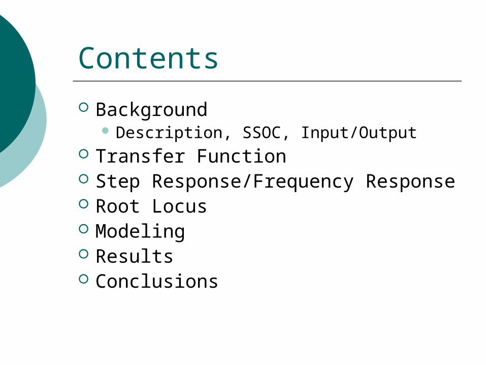
Contents

Background Description, SSOC, Input/Output

Transfer Function Step Response/Frequency Response Root Locus Modeling Results Conclusions

Background - System

                                                                                                                                                         

                       Figure 1. Schematic diagram of the Dunlap Plant Spray-Paint Booths

Background - Block Diagram

                                                                                                                                                   

Figure 2. Block diagram of paint booth system

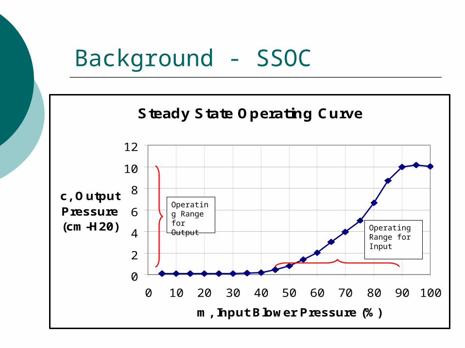
Background - SSOC

Steady State Operating Curve

0

2

4

6

8

10

12

0 10 20 30 40 50 60 70 80 90 100

m, Input Blower Pressure (%)

c, Output Pressure (cm-H20)

Operating Range for Output

Operating Range for Input

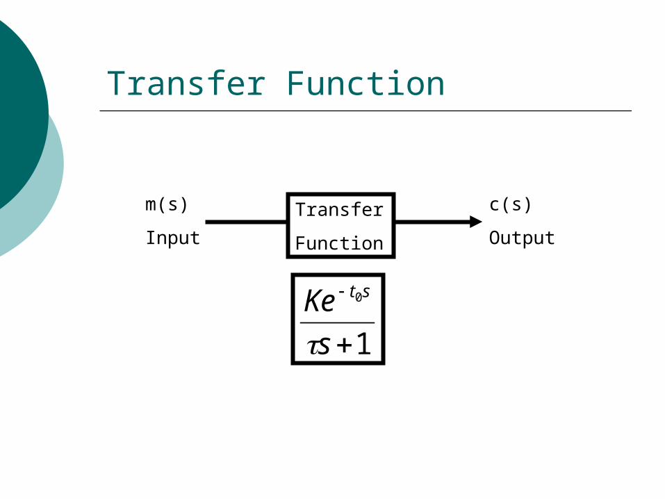
Transfer Function

Transfer

Function

m(s)

Input

c(s)

Output

1

0

s

Ke st

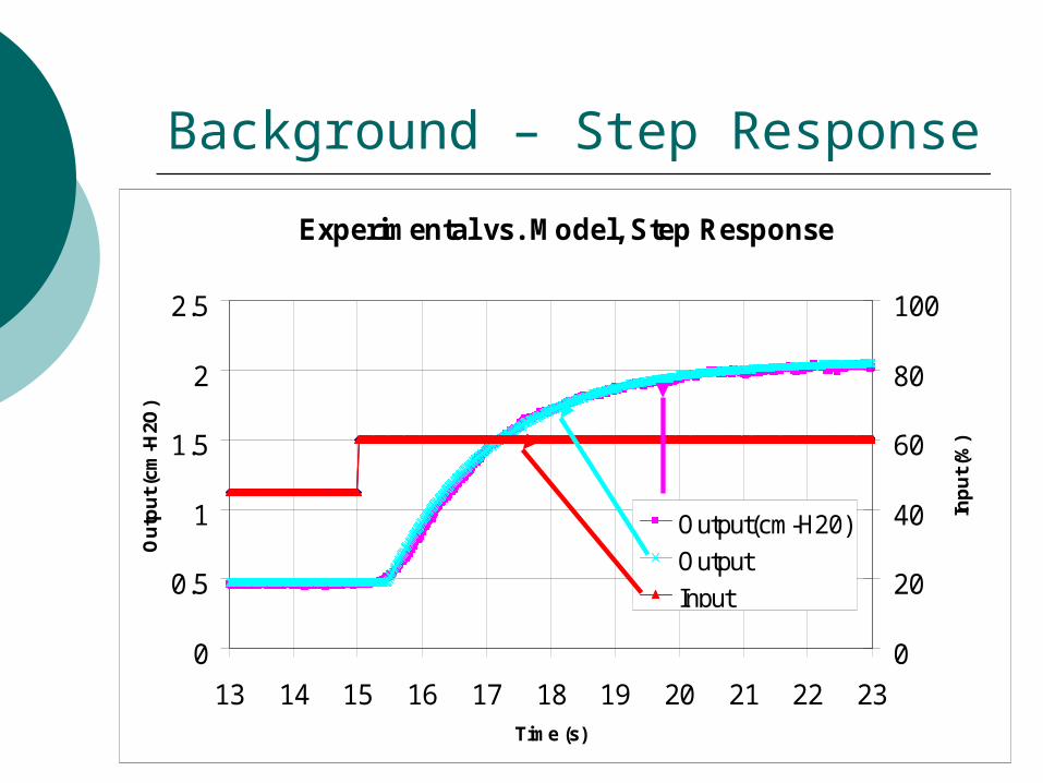
Background – Step Response

Experimental vs. Model, Step Response

0

0.5

1

1.5

2

2.5

13 14 15 16 17 18 19 20 21 22 23Time (s)

Ou

tpu

t (cm

-H2O

)

0

20

40

60

80

100

Inp

ut (

%)

Output(cm-H20)

Output

Input

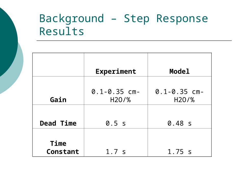
Background – Step Response Results

  Experiment Model

Gain0.1-0.35 cm-

H2O/%0.1-0.35 cm-

H2O/%

Dead Time 0.5 s 0.48 s

Time Constant 1.7 s 1.75 s

Frequency Response - Example

f=0.04, Frequency Response

40

45

50

55

60

65

0 10 20 30 40

Time, s

Inp

ut,

%

0

0.5

1

1.5

2

2.5

Ou

tpu

t, cm

-H2O

Input Value(%)

Output(cm-H20)

c (1.45)

T (25.3)

m (15)

t (-1.8)

Frequency Response – Bode Plots

Bode Plot 75-90% input

-270.00

-180.00

-90.00

0.00

0.01 0.10 1.00

Frquency (Hz)

Pha

se A

ngle

(deg

rees

)

fu=0.85 Hz

)(tan180 10 t

Bode Plot 75-90% input

0.010

0.100

1.000

0.01 0.10 1.00

Frquency (Hz)

Am

plit

ud

e R

ati

o

Frequency Response – Bode Plots

K= 0.35 cm-H2O/%

2nd Order

2

K

f

2

3

fu=0.85

AR=.024

fuARKcu

1

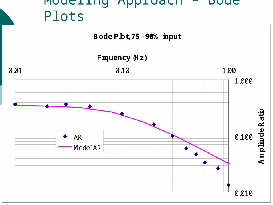
Modeling Approach – Bode PlotsBode Plot, 75 - 90% input

0.010

0.100

1.000

0.01 0.10 1.00

Frquency (Hz)

Am

plit

ud

e R

atio

AR

Model AR

Modeling Approach – Bode PlotsBode Plot, 75 - 90% input

-270.00

-180.00

-90.00

0.00

0.01 0.10 1.00

Frquency (Hz)

Ph

ase

An

gle

(deg

rees

)

PA

Model PA

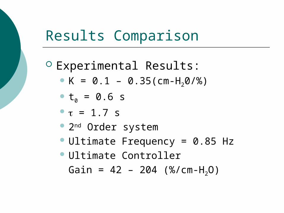
Results Comparison

Experimental Results: K = 0.1 – 0.35(cm-H20/%)

t0 = 0.6 s = 1.7 s 2nd Order system Ultimate Frequency = 0.85 Hz Ultimate Controller

Gain = 42 – 204 (%/cm-H2O)

Results Comparison

Model Results: K = 0.1 – 0.35 (cm-H2O/%)

t0 = 0.85 s = 1.7 s

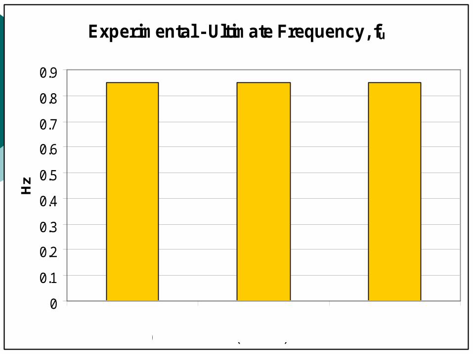
Experimental - Ultimate Frequency, fu

0

0.1

0.2

0.3

0.4

0.5

0.6

0.7

0.8

0.9

Hz

Lower (40-60%)

Middle(60-75%)

Upper(75-90%)

Experimental - Ultimate Controller Gain

0

50

100

150

200

250

%/c

m-H

2O

Middle(60-75%)

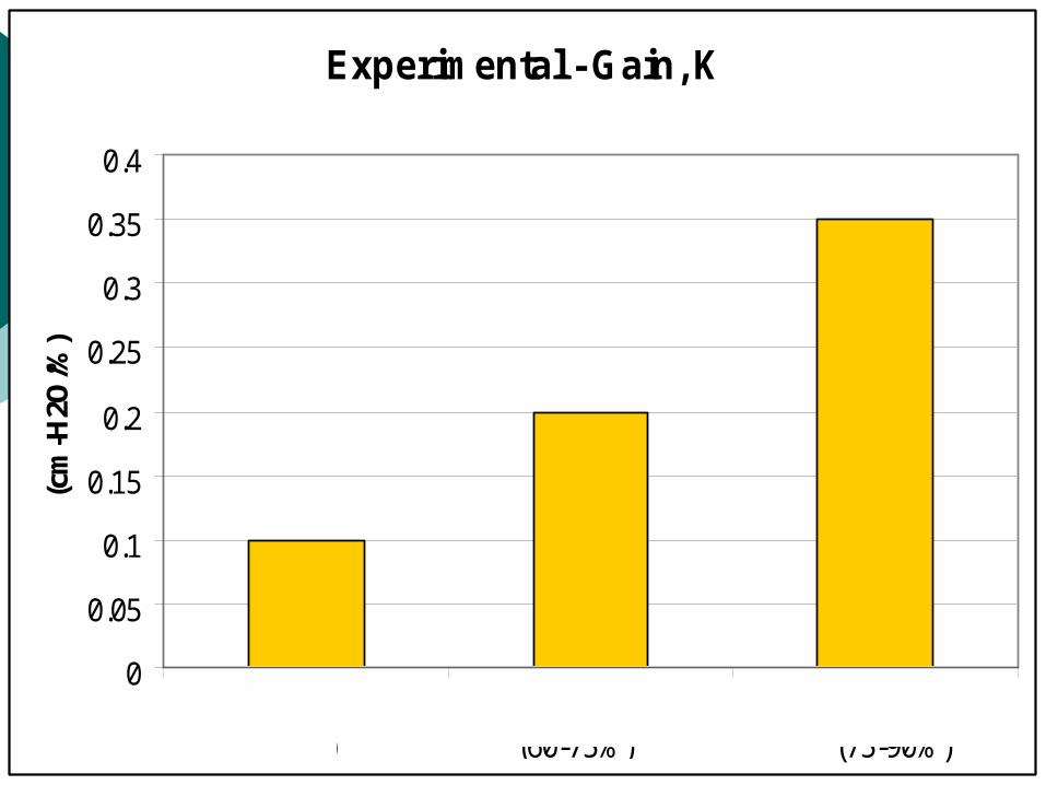
Experimental - Gain, K

0

0.05

0.1

0.15

0.2

0.25

0.3

0.35

0.4

(cm

-H2O

/%)

Lower (40-60%)

Middle(60-75%)

Upper(75-90%)

Experimental - Dead time, t0

0

0.1

0.2

0.3

0.4

0.5

0.6

0.7

seco

nds

Lower (40-60%)

Middle(60-75%)

Upper(75-90%)

Experimental - Time constant,

0

0.2

0.4

0.6

0.8

1

1.2

1.4

1.6

1.8

seco

nds

Lower (40-60%)

Middle(60-75%)

Upper(75-90%)

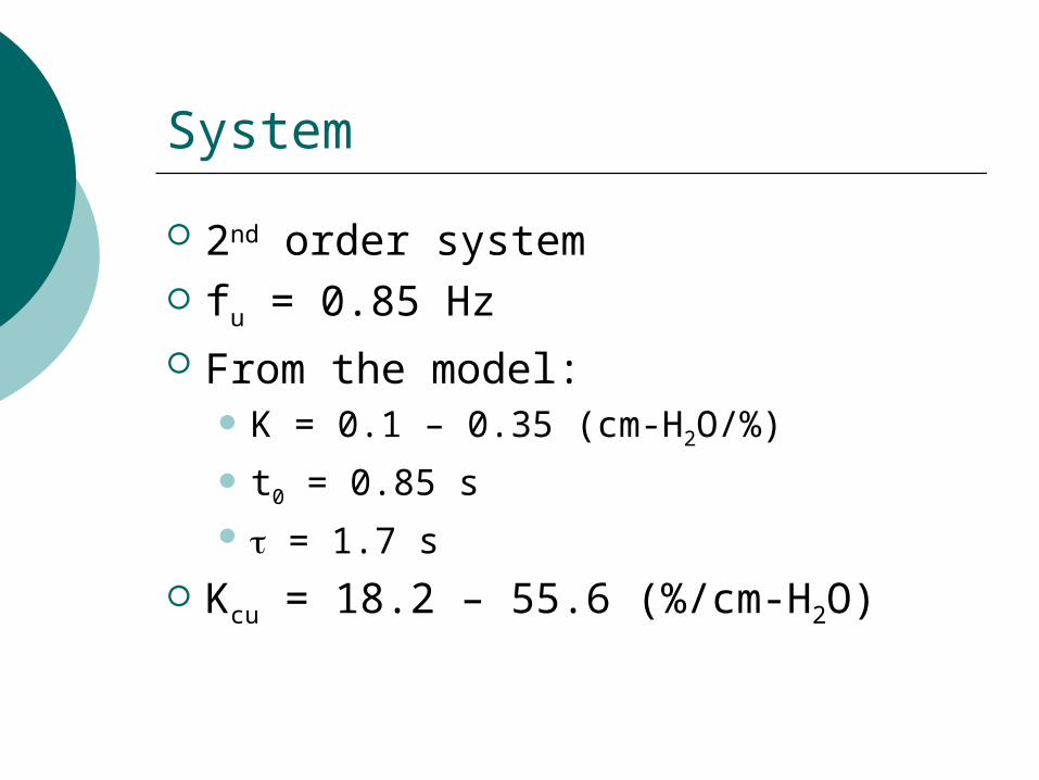
System

2nd order system fu = 0.85 Hz From the model:

K = 0.1 – 0.35 (cm-H2O/%)

t0 = 0.85 s = 1.7 s

Kcu = 18.2 – 55.6 (%/cm-H2O)

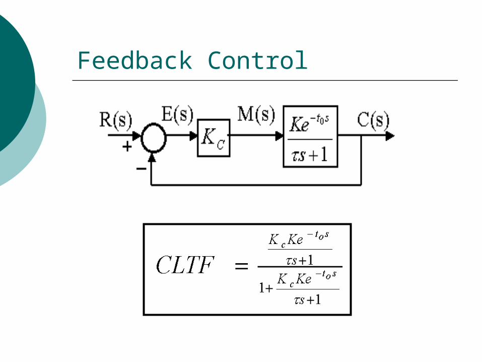
Feedback Control

LocationsROOT LOCUS PLOT

-4

-3

-2

-1

0

1

2

3

4

-2.5 -2 -1.5 -1 -0.5 0 0.5

REAL AXIS

IMA

GIN

AR

Y A

XIS

ξ=1DR=0

ξ=.707DR=1/500

ξ=.344DR=1/10

ξ=.215DR=1/4

ξ=0DR=1

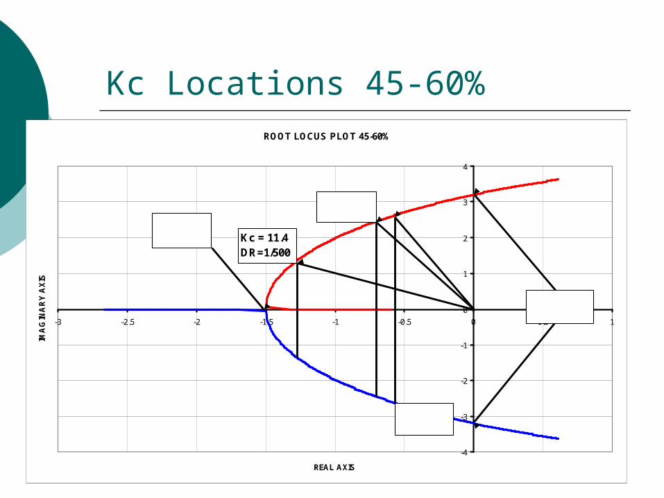
Kc Locations 45-60%ROOT LOCUS PLOT 45-60%

-4

-3

-2

-1

0

1

2

3

4

-3 -2.5 -2 -1.5 -1 -0.5 0 0.5 1

REAL AXIS

IMA

GIN

AR

Y A

XIS

Kc = 11.4DR=1/500

Kc = 36.3DR=1/4

Kc = 27.3DR=1/10

Kc = 4.4DR=0

Kcu = 55.4DR=1

Kc Locations 60-75%

ROOT LOCUS PLOT

-4.00

-3.00

-2.00

-1.00

0.00

1.00

2.00

3.00

4.00

-3.00 -2.50 -2.00 -1.50 -1.00 -0.50 0.00 0.50

REAL AXIS

IMA

GIN

AR

Y A

XIS

Kc=2.2DR=0

Kcu=28DR=1

Kc=18DR=1/4

Kc=16DR=1/10

Kc=5.9DR=1/500

Kc Locations 75-90%

ROOT LOCUS PLOT 75-90%

-4

-3

-2

-1

0

1

2

3

4

-2.5 -2 -1.5 -1 -0.5 0 0.5

REAL AXIS

IMA

GIN

AR

Y A

XIS

Kc=1DR=0

Kc=2.8DR=1/500

Kc=7.9DR=1/10

Kc=8.6DR=1/4

Kc=14DR=1

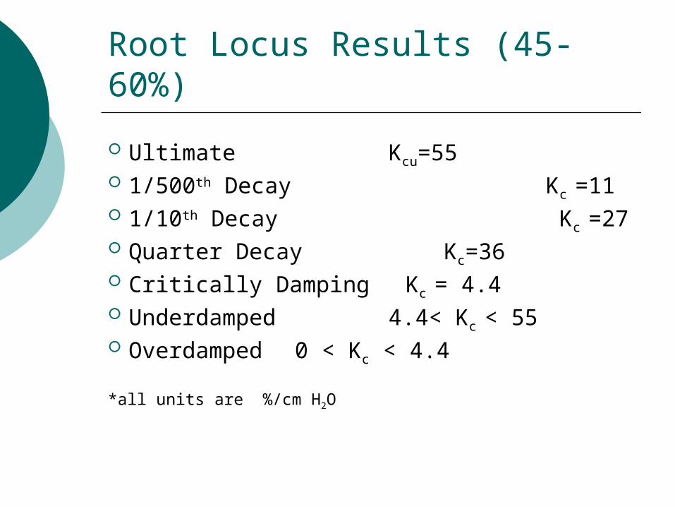
Root Locus Results (45-60%)

Ultimate Kcu=55 1/500th Decay Kc =11 1/10th Decay Kc =27 Quarter Decay Kc=36 Critically Damping Kc = 4.4 Underdamped 4.4< Kc < 55 Overdamped 0 < Kc < 4.4

*all units are %/cm H2O

Root Locus Results (60-75%)

Ultimate Kcu=28 1/500th Decay Kc =5.9 1/10th Decay Kc =16 Quarter Decay Kc=18 Critically Damping Kc = 2.2 Underdamped 2.2< Kc < 28 Overdamped 0 < Kc < 2.2

*all units are %/cm H2O

Root Locus Results (75-90%)

Ultimate Kcu=14 1/500th Decay Kc =2.8 1/10th Decay Kc =7.9 Quarter Decay Kc=8.6 Critically Damping Kc = 1.0 Underdamped 1.0< Kc < 14 Overdamped 0 < Kc < 1.0

*all units are %/cm H2O

Conclusions

For 45-60% Kc needed

Overdamped 0 < Kc < 4.4

Critically Damped Kc = 4.4

Underdamped 4.4< Kc < 55

Quarter Decay Kc = 36

*all units are % / cm H2O

Conclusions

For 60-75% Kc needed

Overdamped 0 < Kc < 2.2

Critically Damped Kc = 2.2

Underdamped 2.2< Kc < 28

Quarter Decay Kc = 18

*all units are % / cm H2O

Conclusions

For 75-90% Kc needed

Overdamped 0 < Kc < 1.0

Critically Damped Kc = 1.0

Underdamped 1.0< Kc < 14

Quarter Decay Kc = 8.6

*all units are % / cm H2O

Conclusions

45-60% 0.69 0.48 0.27 0.22 0.1560-75% 0.69 0.46 0.24 0.22 0.1575-90% 0.74 0.5 0.27 0.25 0.17

1/4th Decay

UltimateOffsetCritical

Damping1/500th Decay

1/10th Decay

rKcK11

Offset=