PHYSICAL REVIEW B 97, 235450 (2018)

Flavor fluctuations in three-level quantum dots: Generic SU(3) Kondo fixed point in equilibriumand non-Kondo fixed points in nonequilibrium

Carsten J. Lindner,1,2 Fabian B. Kugler,3 Herbert Schoeller,1,2,* and Jan von Delft31Institut für Theorie der Statistischen Physik, RWTH Aachen, 52056 Aachen, Germany

2JARA-Fundamentals of Future Information Technology, Aachen, Germany3Physics Department, Arnold Sommerfeld Center for Theoretical Physics, and Center for NanoScience,

Ludwigs-Maximilians-Universität München, Theresienstr. 37, 80333 Munich, Germany

(Received 28 February 2018; published 29 June 2018)

We study a three-level quantum dot in the singly occupied cotunneling regime coupled via a generic tunnelingmatrix to several multichannel leads in equilibrium or nonequilibrium. Denoting the three possible states of thequantum dot by the quark flavors up (u), down (d), and strange (s), we derive an effective model where also eachreservoir has three flavors labeled by u, d , and s with an effective density of states polarized with respect to aneight-dimensional F spin corresponding to the eight generators of SU(3). In equilibrium we perform a standardpoor man’s scaling analysis and show that tunneling via virtual intermediate states induces flavor fluctuations onthe dot which become SU(3) symmetric at a characteristic and exponentially small low-energy scale TK . Closeto TK the system is described by a single isotropic Kondo coupling J > 0 diverging at TK . Using the numericalrenormalization group, we study in detail the linear conductance and confirm the SU(3)-symmetric Kondo fixedpoint with universal conductance G = 3 sin2(π/3) e2

h= 2.25 e2

hfor various tunneling setups by tuning the level

spacings on the dot. We also identify regions of the level positions where the SU(2) Kondo fixed point is obtainedand find a rather complex dependence of the various Kondo temperatures as function of the gate voltage and thetunneling couplings. In contrast to the equilibrium case, we find in nonequilibrium that the fixed-point model is notSU(3) symmetric but characterized by rotated F spins for each reservoir with total vanishing sum. At large voltagewe analyze the F -spin magnetization and the current in Fermi’s golden rule as function of a longitudinal (hz) andperpendicular (h⊥) magnetic field for the isospin and the level spacing � to the strange quark. As a smoking gunto detect the nonequilibrium fixed point we find that the curve of zero F -spin magnetization in (hz,h⊥,�) spaceis a circle when projected onto the (hz,h⊥) plane. We propose that our findings can be generalized to the case ofquantum dots with an arbitrary number N of levels.

DOI: 10.1103/PhysRevB.97.235450

I. INTRODUCTION

Over the last three decades, transport properties of cor-related quantum dots have gained an enormous interest inmany experimental and theoretical research activities in con-densed matter physics. As artificial atoms they allow for acontrolled study of interesting phenomena playing a centralrole in many different fields of applied and fundamentalresearch in nanoelectronics, spintronics, quantum informationprocessing, dissipative quantum mechanics, and many-bodyphysics and nonequilibrium phenomena in correlated systems(see, e.g., Refs. [1,2] for reviews). Of particular interest is thecotunneling or Coulomb blockade regime of quantum dotswith strong charging energy, where the charge is fixed andonly the spin and orbital degrees of freedom can fluctuateby second-order tunneling processes via virtual intermediatestates. In this regime, effective models can be derived whichare equivalent to Kondo models well known from solid-statephysics [3] (see, e.g., Ref. [4] for a review of the Kondoeffect in quantum dots). The standard model is the SU(2)Kondo model, where a local spin- 1

2 is coupled via an isotropic

*schoeller@physik.rwth-aachen.de

exchange coupling to the spins of two large reservoirs. Below acharacteristic low-energy scale, called the Kondo temperatureTK , the local spin is completely screened and the remainingpotential scattering leads to resonant transport through thesystem with universal conductance 2 e2

h. This Kondo effect

has been theoretically predicted for quantum dots [5] and hasbeen experimentally observed [6]. After this discovery, theresearch for Kondo physics in quantum dots has gained anenormous interest and further realizations have been proposedand observed, such as, e.g., the realization of higher spin values[7], singlet-triplet fluctuations [8], non-Fermi-liquid behaviorin two-channel realizations [9], and the SU(4) Kondo effect[10]. Recently, also the realization of SU(N ) Kondo physicsfor arbitrary N has been proposed in coupled quantum dots[11–13].

The enormous variety of possible realizations of Kondophysics raises the question as to what happens in the genericcase when a quantum dot in the regime of fixed charge withNdot � 1 electrons and N � 2 levels is coupled via a generictunneling matrix to several multichannel reservoirs. Even forthe simplest case Ndot = 1 and N = 2, this issue is nontrivialsince the quantum number l = 1,2 labeling the two dot levelsis in general a nonconserved quantity in tunneling, such as,e.g., for ferromagnetic leads [14], orbital degrees of freedom

2469-9950/2018/97(23)/235450(21) 235450-1 ©2018 American Physical Society

LINDNER, KUGLER, SCHOELLER, AND VON DELFT PHYSICAL REVIEW B 97, 235450 (2018)

[15], Aharonov-Bohm geometries [16], and spin-orbit orDzyaloshinski-Moriya interactions [17,18]. In Ref. [16] itwas shown via a singular value decomposition of the totaltunneling matrix (i.e., containing all reservoirs) that all thesedifferent cases can be mapped onto an effective model which isequivalent to the anisotropic spin- 1

2 Kondo model which flowsinto the isotropic SU(2)-symmetric fixed point at low energiesbelow the Kondo temperature. This explains why in alllinear response transport calculations of quantum dot modelswith Ndot = 1 and N = 2, the Kondo effect with universalconductance is observed provided that local effective magneticfields are explicitly canceled by external ones [19]. However,this result is only valid in the linear response regime and forproportional couplings to all the reservoirs where the linearconductance can be related to the equilibrium spectral densityof the dot [20]. To calculate the latter, all reservoirs can be takentogether to a single one and only the total tunneling matrixmatters. However, when all reservoirs are coupled in a genericway to the dot or when they are characterized by differenttemperatures or chemical potentials, the analysis of Ref. [16] isno longer valid. This fact was emphasized in Ref. [21], whereit was shown that in a generic nonequilibrium situation, theproper effective model for Ndot = 1 and N = 2 is a spin-valvemodel, where the spin polarizations of all reservoirs point indifferent directions, such that at the low-energy fixed pointtheir sum is equal to zero. This has the consequence that thefixed-point model in nonequilibrium is essentially not SU(2)symmetric and new interesting nonequilibrium fixed-pointmodels emerge with different non-Kondo-type properties inthe weak- as well as in the strong-coupling regime. Only inthe equilibrium situation when all reservoirs are characterizedby the same temperature and chemical potential, all reservoirscan be taken together, resulting in an unpolarized reservoirwith SU(2) symmetry at the fixed point. The nonequilibriumproperties at and away from the fixed-point model have beenstudied for large voltages above the Kondo temperature [21],and a smoking gun was identified in the nontrivial magneticfield dependence of the magnetization and the transportcurrent characterizing the fixed-point model.

The proposals of new nonequilibrium fixed-point modelsare of particular interest for the constant effort to generalizewell-established analytical and numerical methods for thestudy of equilibrium properties of quantum impurity models[3,22] to the nonequilibrium case. Recent developments ofperturbative renormalization group methods [23–26] haveshown how the voltage dependence and the physics of cutoffscales by decay rates can be implemented [27] and how thetime evolution into the stationary state can be calculated[28]. Even in the strong-coupling regime [29,30] results inagreement with experiments [31] were obtained, although theused methods are essentially perturbative and not capable ofdescribing the strong-coupling regime in general. Therefore,numerically exact methods are required for the descriptionof quantum dot systems in nonequilibrium, such as, e.g., thetime-dependent numerical renormalization group (TD-NRG)[32], time-dependent density matrix renormalization group(TD-DMRG) [33], iterative stochastic path integrals [34], andquantum Monte Carlo methods [35]. Recently, a promisingthermofield approach has been suggested by a combinationof TD-NRG and TD-DMRG [36] showing a good agreement

with the strong-coupling results for the nonequilibrium Kondomodel of Refs. [29–31].

The aim of this paper is to analyze the generic case Ndot = 1and arbitrary N to see how the results of Ref. [21] can begeneralized to the case N > 2. In particular, we will study thecase N = 3 and, starting from a generic tunneling matrix, willshow that an effective tunneling model can be derived wherealso the reservoirs are characterized by three flavors which wewill conveniently label by the up (u), down (d), and strange(s) quark flavors. The effective model in the cotunnelingregime of a singly occupied quantum dot can be described byflavor fluctuations, and we will show by a poor man’s scalinganalysis that the low-energy fixed-point model is indeed theSU(3)-symmetric Kondo model. This result is shown to holdalso for arbitrary N within the poor man’s scaling analysisand will be explicitly confirmed for N = 3 by a numericallyexact NRG analysis for the linear response conductance,similiar to Refs. [12,13]. In addition to these references, wewill study the dependence of the SU(3) Kondo temperatureon the tunneling matrix elements and will show how theSU(3)-symmetric point is obtained by a proper adjustment ofthe level spacings of the dot. Subsequently, we will analyzethe nonequilibrium situation and generalize the spin-valvemodel of Ref. [21] for N = 2 to the case of three levelsN = 3. In this case, a fixed-point model arises where thereservoirs are characterized by eight-dimensional F spinscorresponding to the eight generators of the SU(3) group whichcancel when all reservoirs are taken together. For large voltagesand two reservoirs we find that the nonequilibrium fixed-pointmodel has a characteristic dependence on the dot parametersfor zero F -spin magnetization on the dot providing a smokinggun for the detection of the fixed point. Thus, we concludethat the results of Ref. [21] can indeed be generalized to thecase of N > 2 levels with a great potential for a variety of newinteresting nonequilibrium fixed-point models where the low-energy behavior in the strong-coupling regime is still unknown.

The paper is organized as follows. In Sec. II we will derivevarious effective models. We will set up effective tunnelingmodels in Sec. II A and the effective model in the cotunnelingregime in Sec. II B. The fixed-point model is obtained via a poorman’s scaling analysis in Sec. II C for arbitrary N . In Sec. II Dwe consider the particular case N = 3 and will set up the rela-tion to the representation of the SU(3) group and the physicalpicture in terms of F -spin interactions. In Sec. III we will usethe NRG method to confirm the SU(3)-symmetric fixed-pointmodel in the linear response regime. Finally, in Sec. IV weanalyze the nonequilibrium properties of the fixed-point modelin the perturbative regime of large voltage via a Fermi’s goldenrule approach. The general formulas are derived in Sec. IV Aand the magnetization and the current are calculated as functionof characteristic dot parameters for the case of two reservoirsin Sec. IV B where the smoking gun for the detection of thefixed-point model is derived. We close with a summary of ourresults in Sec. V. We use units e = h = 1 throughout this paper.

II. DERIVATION OF EFFECTIVE MODELS

In this section we start from a quantum dot with N levelscoupled via a generic tunneling matrix to Nres multichannelnoninteracting reservoirs in grand-canonical equilibrium. We

235450-2

FLAVOR FLUCTUATIONS IN THREE-LEVEL QUANTUM … PHYSICAL REVIEW B 97, 235450 (2018)

show in Sec. II A that this model is equivalent to an effectiveone where the number of channels in each reservoir is the sameas the number N of the quantum dot levels. For the specialcase of N = 3 this sets the basis to use a notation in terms ofthree flavor states for the three channels and to characterizethe reservoirs by rotated F spins with a certain isospin andhypercharge polarization. In addition, we will set up variouseffective tunneling models and characterize the properties ofthe central fixed-point model derived in Secs. II B–II D for thecotunneling regime, where the number Ndot of particles onthe dot is fixed to Ndot = 1, such that only flavor fluctuationsvia virtual intermediate states can occur. In this regime, wewill derive an effective model describing flavor fluctuationsand propose the fixed-point model from a poor man’s scalinganalysis.

A. Effective tunneling models

The starting point is a quantum dot consisting of N lev-els characterized by some quantum number l = 1,2, . . . ,N ,together with a Coulomb energy ENdot depending only on thetotal particle number operator Ndot =∑l c

†l cl of the dot

Hdot =∑ll′

hll′c†l cl′ + ENdot , (1)

ENdot = EC(Ndot − nx)2, (2)

where c†l /cl are the creation/annihilation operators of the

single-particle states of the dot. The charging energy Ec isassumed to be the largest energy scale in the problem such that,for small hll′ , the parameter nx determines the occupation ofthe dot. If nx = n is integer, the ground state will be dominatedby Ndot = n, whereas for half-integer nx = n + 1

2 , states withNdot = n,n + 1 are degenerate with respect to the Coulombinteraction. For convenience, we define the gate voltage by

Vg = Ec(2nx − N ), (3)

such that Vg = 0 (or nx = N/2) defines the particle-hole-symmetric point for hll′ = 0. With this definition we can alsowrite the dot Hamiltonian in second quantized form as

Hdot =∑ll′

hll′c†l cl′ + U

2

∑ll′

c†l c

†l′cl′cl, (4)

with U = 2Ec and hll′ = hll′ − [Vg + (U/2)(N − 1)]δll′ .The quantum dot is coupled via a generic tunneling matrix

to several infinitely large reservoirs α = 1,2, . . . ,Nres kept atgrand-canonical equilibrium with temperature T and chemicalpotential μα , such that the total Hamiltonian reads as

Htot = Hdot + Hres + HT , (5)

with the reservoir Hamiltonian

Hres =∑αναk

εαναk a†αναkaαναk, (6)

and the tunneling Hamiltonian

HT = 1√ρ(0)

∑αναlk

{tαναla

†αναkcl + (tαναl

)∗c†l aαναk

}. (7)

Here, να = 1,2, . . . ,Nα is the channel index for reservoir α

(with Nα channels in total), εαναk is the band dispersion ofreservoir α for channel να relative to the chemical potentialμα and labeled by k (which becomes continuous in thethermodynamic limit), and tαναl is the tunneling matrix betweenthe dot and reservoir α. ρ(0) is some average density ofstates (DOS) in the reservoirs, which is set to ρ(0) = 1 in thefollowing defining the energy units. In vector-matrix notation,the tunneling Hamiltonian can be written in a more compactform as

HT =∑αk

{a†αk t

αc + c† t†

αaαk}, (8)

where c† = (c†1, . . . ,c†N ), a

†αk = (a†

α1k, . . . ,a†αNαk), and t

αis a

Nα × N matrix with matrix elements tαναl . For convenience,we have taken here a tunneling matrix independent of k whichis usually a very good approximation for rather flat reservoirbands on the scale of the low-energy scales of interest.

Using Keldysh formalism. it is straightforward [20,37] torelate the stationary current Iανα

in reservoirα and channel να tothe stationary nonequilibrium greater/lesser Green’s functionsG

≷ll′ (ω) of the dot via

Iανα= e

h

∫dω Tr

ανα

{[1 − fα(ω)] iG<(ω)

+ fα(ω) iG>(ω)}, (9)

where Tr denotes the trace over the single-particle states ofthe dot, fα(ω) = (eβ(ω−μα) + 1)−1 is the Fermi function ofreservoir α, and the (N × N )-hybridization matrix

ανα

isdefined by (

ανα

)ll′ = 2πρανα

(tαναl

)∗tαναl′ . (10)

Here, ρανα=∑k δ(ω − εαναk) denotes the DOS in reservoir

α for channel να , which is assumed to be rather flat so thatthe energy dependence can be neglected. The influence ofthe reservoirs and the tunneling on the Green’s functions isdetermined by the reservoir part of the lesser/greater self-energy given by

�<

res(ω) = i

∑α

fα(ω)α, (11)

�>

res(ω) = −i

∑α

(1 − fα(ω))α, (12)

where

α

=∑να

ανα

= 2π t†αρ

αtα

(13)

is the hybridization matrix for reservoir α including all chan-nels and (ρ

α)ναν ′

α= δναν ′

αρανα

is the diagonal matrix for the

DOS of reservoir α. As a consequence, we see that the Green’sfunctions depend on the reservoirs and the tunneling matrixonly via the hybridization matrices

αof all the reservoirs.

Thus, two models with the same hybridization matrices giveexactly the same Green’s functions. Once the Green’s functionsare known, the channel-resolved currents Iανα

can be calculatedfrom (9), where the channel-resolved hybridization matrix

ανα

of the concrete model under consideration has to be

235450-3

LINDNER, KUGLER, SCHOELLER, AND VON DELFT PHYSICAL REVIEW B 97, 235450 (2018)

inserted. The stationary expectation values of single-particleoperators of the dot can be directly calculated from the lesserGreen’s functions via 〈c†l′cl〉 = 1

2πi

∫dω G<

ll′(ω) and thus areexactly the same for two models with the same hybridizationmatrices

α.

We note that for the equilibrium case, where all Fermifunctions of the reservoirs are the same, the reservoir self-energies involve only the total hybridization matrix

=∑

α

α, (14)

with the result that the equilibrium Green’s functions are thesame for two models with the same . However, the current inlinear response can not be related to the single-particle Green’sfunctions in equilibrium via (9) since also the Green’s functionshave to be expanded in the voltages. A special case is the oneof proportional couplings where it is assumed that

α= xα

with∑

α xα = 1. Using current conservation∑

α Iα = 0, withIα =∑να

Iαναdenoting the total current in reservoir α, we get

in this case from (9) the Landauer-Büttiker–type formula [20]

Iα = e

h

∑β �=α

∫dω Tαβ(ω)(fα − fβ)(ω), (15)

with the transmission probability

Tαβ(ω) = 2π xαxβTr ρ(ω), (16)

where ρ(ω) = i2π

(GR − GA)(ω) is the spectral density on the

dot. From this formula one can see that in linear response,where (fα − fβ)(ω) ≈ −f ′(ω)(μα − μβ), one needs only thespectral density in equilibrium and, with μα = −eVα , thecurrent can be written as

Iα =∑

β

Gαβ(Vβ − Vα), (17)

with the conductance tensor

Gαβ = −e2

h

∫dω Tαβ(ω) f ′(ω). (18)

With the knowledge that the hybridization matrices α

are the only input we need to characterize the reservoirs andthe tunneling matrix, we can now proceed to define effectivemodels with the same hybridization matrices. Since

αis a

positive-definite Hermitian matrix, we can diagonalize it witha unitary matrix U

α,

α

= Uαd

αU †

α, (19)

where (dα)ll′ = δll′αl is a diagonal matrix with positive

eigenvalues αl = 2πt2αl > 0. We exclude here the exotic case

that one of the eigenvalues αl is zero since this wouldmean that one of the reservoir channels effectively decouplesfrom the system. Following Ref. [21], we can write thehybridization matrix in two equivalent forms by shifting thewhole information either to an effective tunneling matrix orto an effective DOS of the reservoirs. In the first case, weintroduce an effective tunneling matrix teff

αby(

teffα

)ll′ = tαl(U

†α)ll′ (20)

and get

α

= 2π(teffα

)†teffα

. (21)

Since teffα

is an N × N matrix, this effective model consists ofreservoirs which have exactly the same number N of channelsas we have levels on the dot, i.e., the quantum number on thedot is also the quantum number labeling the channels in theeffective reservoirs but this quantum number is in general notconserved by tunneling. Comparing (21) to (13), we see thatthe effective DOS in the reservoirs is unity, i.e., we considerunpolarized reservoirs.

In the second case, we define an effective DOS ρeff

αin

reservoir α by

ρeff

α= N U

α

(d

α

/α

)U †

α, (22)

with α =∑l αl . Defining an average tunneling matrixelement tα > 0 by t2

α = 1N

∑l t

2αl , we can then write the

hybridization matrix as

α

= 2πt2α ρeff

α. (23)

In this case, the effective tunneling matrix is proportionalto unity, the tunneling conserves the flavor and is flavorindependent. In contrast, the effective DOS contains thewhole nontrivial information of the hybridization matrix anddescribes a unitary transformation of the diagonal matrixN d

α/α . The latter matrix can be decomposed in a basis

of all diagonal matrices and the coefficients can be interpretedas physical parameters characterizing the effective reservoirs.Using Tr d

α= α , we get for N = 2

2 d

α/α = 1

2+ pασ

z, (24)

where σz is the Pauli matrix in the z direction and pα describesthe spin polarization in reservoir α. Since the matrix has onlypositive diagonal elements we get the condition −1 < pα < 1.If one orders the eigenvalues according to α1 � α2, one gets0 < pα < 1.

For N = 3 we obtain

3 dα/α = 1

3+ pαλ

3+ qα√

3λ

8, (25)

where

λ3

=⎛⎝1 0 0

0 −1 00 0 0

⎞⎠, (26)

λ8

= 1√3

⎛⎝1 0 0

0 1 00 0 −2

⎞⎠ (27)

are the two diagonal generators of the SU(3) group, de-scribing the isospin in z direction of the up/down quark andthe hypercharge operator Y = 1√

3λ

8, respectively. Therefore,

we interpret pα as the isospin polarization and qα as thehypercharge polarization characterizing the reservoirs in thethree-channel case. The fact that all matrix elements of (25)are positive leads to the two conditions

|pα| < 1 + qα

3, 0 < 1 + qα

3<

3

2. (28)

235450-4

FLAVOR FLUCTUATIONS IN THREE-LEVEL QUANTUM … PHYSICAL REVIEW B 97, 235450 (2018)

pL, qL

fL

µL = eV2

pR, qR

fR

µR = −eV2

|u

|d

|s

hzh⊥

Δ

ΓL = xLΓ ΓR = xRΓ

FIG. 1. Sketch of the effective model of two F -spin polarizedleads α = L,R coupled to a three-level quantum dot via flavor-conserving tunneling rates L,R = xL,R. μL,R = ±eV/2 denote thechemical potentials of the leads with eight-dimensional F spins f

L,R

characterized by an isospin polarization pL,R and hypercharge polar-ization qL,R . h = (h⊥,hz) with h⊥ = (hx,hy) denotes the magneticfield acting on the two isospin dot levels (up and down quarks), and� is the level spacing between the strange quark and the average ofthe two isospin levels.

If one orders the eigenvalues according to α1 � α2 � α3,one gets 0 < pα < qα < 3

2 .The unitary transformation U

αdescribes a rotation of the

direction of the spin- 12 in the N = 2 case, and a rotation of

the eight-dimensional F spin with Fi= 1

2λi

for N = 3 (seeFig. 1 for an illustration). Thus, the form (23) allows for anice physical interpretation in terms of physical parameterscharacterizing the reservoirs. For N = 3, we can label the threeflavors of the reservoirs and the dot by l = u,d,s for the up,down, and strange quark and describe with the form (23) asystem where the flavor is conserved in tunneling with equaltunneling amplitudes for all flavors. However, the polarizationpα of the isospin described by the up and down quarks and thehypercharge polarization qα can be different for each reservoir,and the F spins in the reservoirs can all be rotated relative tothe F spin of the dot. This naturally generalizes the effectivespin-valve model set up in Ref. [21] for N = 2 to the N = 3case, which is the main subject of this paper.

The form (21) in terms of an effective tunneling matrixallows for another representation of the hybridization matrixwhich will turn out to be crucial to interpret the fixed-pointmodel derived in Sec. II C for the cotunneling regime. Takingall effective tunneling matrices together in a N · Nres × N

matrix

teff =

⎛⎜⎜⎜⎜⎝

teff1···

teffNres

⎞⎟⎟⎟⎟⎠, (29)

we can write this matrix via a singular value decomposition as

teff = V

(γ

0

)W †, (30)

where V is a unitary N · Nres × N · Nres matrix, γ is an

N × N diagonal matrix containing the positive singular values

γ1 � γ2 � · · · � γN > 0, and W is a unitary N × N matrix.We assume here that N singular values exist, excludingexotic cases where some channels decouple effectively fromthe system. As a consequence, we can express all effectivetunneling matrices in terms of the singular value matrix γ as

follows:

teffα

= Vαγ W †, (31)

where Vα

are the N × N matrices occurring in the first N

columns of V , which are in general not unitary. However, sinceV is unitary, we note the important property

∑α

V †αV

α= 1. (32)

The unitary matrix W can be eliminated by transforming thebasis of the single-particle states of the dot using new fieldoperators c′ = W †c, such that the dot Hamiltonian (1) and thetunneling Hamiltonian (8) obtain the form

Hdot = (c′)†h′c′ + ENdot , (33)

HT =∑αk

{a†αk

(teffα

)′c′ + (c′)†

((teffα

)′)†aαk

}, (34)

with h′ = W † h W and

(teffα

)′ = Vαγ . (35)

For simplicity, we will drop the prime in the following andreplace h′ → h and (teff

α)′ → teff

αkeeping in mind that these

matrices result from the matrices of the original model bytransforming the dot channels with the unitary matrix W .

In terms of the effective tunneling matrices (35), the hy-bridization matrices (21) obtain the form

α

= 2π γ V †α

Vα

γ . (36)

This form is of particular interest since it separates thehybridization matrix in a part γ which is independent of the

reservoirs and a reservoir-dependent part V †αV

α. Comparing

(36) with (13), we can interpret γ as an effective tunneling

matrix which conserves the flavor index and is the samefor all reservoirs. This effective tunneling matrix containsthe information of the eigenvalues l = 2πγ 2

l of the totalhybridization matrix since we get from (32)

=∑

α

α

= 2π γ 2. (37)

The reservoir-dependent part V †αV

αcan be interpreted as an

effective DOS of the reservoirs. Taking N = 3 and decompos-ing this Hermitian matrix in the basis of the F -spin generatorsF

i= 1

2λi

of SU(3) we get

V †αV

α= xα

(1 +

8∑i=1

diα F

i

), (38)

235450-5

LINDNER, KUGLER, SCHOELLER, AND VON DELFT PHYSICAL REVIEW B 97, 235450 (2018)

with real coefficients xα and diα which, due to (32), fulfill the

property ∑α

xα = 1,∑

α

xαdiα = 0. (39)

This means that the sum of the F spins of all reservoirs is zero.A similiar property holds for arbitrary N . In equilibrium, whereall chemical potentials μα = μ are the same and all reservoirscan be taken together to one big reservoir, this means that anunpolarized reservoir with SU(3) symmetry couples to the dot.However, since the effective tunneling matrix elements γl stilldepend on the flavor index, SU(3) symmetry does not hold forthe total system even in equilibrium.

Most importantly, we will see in Sec. II C by a poor man’sscaling analysis in the cotunneling regime of a singly occupieddot Ndot = 1 that a generic fixed-point model with an isotropicmatrix γ = γ 1 emerges, such that the effective tunneling

matrix (35) reads as

teffα

= γVα. (40)

γ > 0 can be related to an isotropic Kondo coupling J via

γ 2 = 1

4JD,

1

D= 1

2

(1

E0+ 1

E2

), (41)

where ENdot is given by (2) and J fulfils the poor man’s scalingequation

dJ

d�= −N

2

J 2

�, (42)

with � denoting the effective bandwidth. In addition, a specialpotential scattering term emerges in the original tunnelingmodel at the fixed point which is given by

Vsc = vsc

∑kk′

∑αα′

: a†αk V

αV †

α′ aα′k′ : , (43)

where

vsc = γ 2

D

(N − 2

N+ δ

), δ = E0 − E2

E2 + E0, (44)

with E0 and E2 from (2), and : · · · : denotes normal ordering.This potential scattering term vanishes for N = 2 and δ = 0(i.e., nx = 1 where E0 = E2) and is such that it cancels thepotential scattering term emerging in an effective model forthe cotunneling regime (see Sec. II B). Due to Vsc, the reservoirpart of the self-energy of the dot is more complicated than (11)and (12) and does not only depend on the hybridization matrix.However, as is shown in Appendix A, the effect of Vsc is justthat γ is changed to an effective γ given by

γ = γ√1 + π2v2

sc

, (45)

such that the self-energies (11) and (12) from the reservoirs canbe written at the fixed point with effective hybridization ma-trices which can be either expressed via an effective tunnelingmatrix analog to (21):

α

= 2π(teffα

)†teffα

, teffα

= γ Vα, (46)

such that the DOS of the reservoirs is unity, or via an effectiveDOS analog to (23),

α

= 2πγ 2 ρeff

α, ρeff

α= V †

αV

α, (47)

with a trivial tunneling matrix given by γ 1 which is the samefor all reservoirs and proportional to unity with respect to theflavor indices. The particular property of the effective DOS atthe fixed point is the condition∑

α

ρeff

α= 1, (48)

following from (32). This means that in contrast to the generalcase depicted in Fig. 1 for N = 3, the particular property of thefixed-point model is that the sum over all reservoir F spins isequal to zero and the tunneling matrix γ = γ 1 is isotropic. As

a consequence, we get overall SU(3) symmetry in equilibrium,whereas in nonequilibrium the fixed-point model is essentiallynot SU(3) symmetric since the F spins of the reservoirs arenonzero. A similar statement holds for any number N of dotlevels, generalizing the picture found in Ref. [21] for N = 2to a generic multilevel quantum dot.

We note that for the particular case of two reservoirs Nres =2 with α = L,R, we get from (32) that V †

LV

L= 1 − V †

RV

R,

such that we can find a common unitary matrix UV

which

diagonalizes both V †αV

αfor α = L,R

V †αV

α= U

VAd

αU †

V, (49)

where Adα

are diagonal matrices with the property

∑α=L,R

Adα

= 1. (50)

For N = 3, the matrix Adα

can be decomposed analog to (25)as

Adα

= xα

(1

3+ pαλ

3+ qα√

3λ

8

), (51)

where, due to the property (50), we get

1 = xL + xR, (52)

0 = xLpL + xRpR, (53)

0 = xLqL + xRqR, (54)

together with 0 < xα < 1 and (28). Thus, the hybridizationmatrices at the fixed point obtain the following form for tworeservoirs:

α

= 2πγ 2 UV

Adα

U †V. (55)

Omitting the unitary matrix UV

by choosing a different single-particle basis for the dot states and redefining the parametershll′ [analog to the transformation by the unitary matrix W , see(33) and (34)], we get finally the diagonal form

α

= 2πγ 2 Adα, (56)

235450-6

FLAVOR FLUCTUATIONS IN THREE-LEVEL QUANTUM … PHYSICAL REVIEW B 97, 235450 (2018)

which, for N = 3, by inserting the decomposition (51), can bewritten as

α

= 1

3α

(1

3+ pαλ

3+ qα√

3λ

8

), (57)

with α = 2πγ 2xα . This form for the hybridization matricesconstitutes the central generic fixed-point model for N = 3and two reservoirs in the cotunneling regime of a singlyoccupied dot. This will be confirmed in Sec. III by NRG inequilibrium and analyzed in Sec. IV by a golden rule approachin nonequilibrium. It generalizes the spin-valve model fora two-level quantum dot with opposite spin polarizations inthe two reservoirs analyzed in Ref. [21] to the case of athree-level quantum dot, where the isospin and hyperchargepolarizations have to be opposite in the two reservoirs. Ananalog fixed-point model arises for an arbitrary number of dotlevels, in this case one obtains in the two reservoirs oppositeparameters corresponding to the N − 1 diagonal generatorsof SU(N ). Whereas in equilibrium the fixed-point model isSU(N ) symmetric (at least if the dot parmeters hll′ are adjustedproperly, see Sec. III) and leads generically to the SU(N )Kondo effect, the nonequilibrium fixed-point model is notSU(N ) symmetric and generically non-Kondo physics has to beexpected. This will be analyzed in Sec. IV in the perturbativegolden rule regime of large voltage, where we will see thatzero F -spin magnetization on the dot occurs only for particularvalues of the dot parameters hll′ providing a smoking gun forthe detection of the fixed-point model.

B. Effective model in the cotunneling regime

The effective model in the cotunneling regime where theparticle number on the dot is fixed to Ndot = 1 can easily beobtained by projecting the Hamiltonian matrix on this subspaceanalog to Brillouin-Wigner perturbation theory. Taking onlyone virtual process into the particle number sectors Ndot = 0,2into account we get

H efftot = Hres + P1HdotP1 − : P1HT Q1

1

HdotQ1HT P1 : ,

(58)

where P1 projects onto the one-particle subspace of the dot andQ1 = 1 − P1. We have introduced the normal-ordering : · · · :with respect to the reservoir field operators since we are notinterested in terms renormalizing the dot Hamiltonian leadingto effective parameters hll′ . For Hres and HT , we take a modelwith the effective tunneling matrix (35) and the unity matrixfor the effective DOS in the reservoirs, as has been discussedin Sec. II. Inserting Hdot and HT from (1) and (8) and usingENdot from (2) we get with P1c

†l cl′P1 = |l〉〈l′|:

H efftot = Hres +

∑ll′

hll′ |l〉〈l′| + E1

− 1

E2

∑αα′

∑kk′

: P1a†αk teff

αc c†(teffα′

)†aα′k′P1 : (59)

− 1

E0

∑αα′

∑kk′

: P1c† (teff

α′

)†aα′k′ a

†αk teff

αcP1 : . (60)

Using

P1(c c†)ll′P1 = −|l′〉〈l| + δll′P1,

: (aα′k′ a†αk)l′l : = − : a

†αlkaα′l′k′ : , (61)

we get after inserting (35) for the tunneling matrix and leavingout the unimportant constant E1

H efftot = Hres +

∑ll′

hll′ |l〉〈l′| + Veff, (62)

with the effective interaction

Veff =∑αα′

∑kk′

: a†αk V

αJ V †

α′ aα′k′ : (63)

and

Jll′ = γlγl′

(2

D|l′〉〈l| − 1

E2δll′ 1

), (64)

with 2/D = 1/E0 + 1/E2 [see (41)]. We note that the hat onJll′ indicates that this object is a dot operator in the one-particlesubspace for each fixed value of l and l′, i.e., J represents aN × N matrix with dot operators in each matrix element. Byusing 1 =∑l |l〉〈l|, a straightforward calculation leads to thedecomposition

Jll′ = ξll′ |l′〉〈l|(1 − δll′ )

+∑l1 �=l

ηll1

(1

N1 − |l1〉〈l1|

)δll′ + vlδll′ 1, (65)

with

ξll′ = 2

Dγlγl′ , ηll′ = 2

Dγ 2

l , (66)

vl = − 1

Dγ 2

l

(N − 2

N+ δ

), (67)

and 2δ = D/E2 − D/E0 [see (44)]. We note that the bareparameters ηll′ are independent of l′ but obtain a strong depen-dence on l′ under the renormalization group flow described be-low. The decomposition (65) exhibits the nondiagonal matrix|l′〉〈l| for l �= l′, all traceless diagonal matrices 1

N1 − |l1〉〈l1|

for l1 �= l, and the unity matrix 1 describing the effectivepotential scattering.

We note that the effective interaction (63) can also be writtenin terms of reservoir field operators for a single reservoir only:

Veff =∑kk′

: a†k J ak′ : , (68)

where

ak =∑

α

V †αaαk (69)

fulfill commutation relations of field operators for a singleeffective reservoir with N flavors due to the property (32).However, this is only possible if all the reservoirs can betaken together, i.e., they must have the same temperature andchemical potential. In nonequilibrium this is not possible.Nevertheless, for the poor man’s scaling analysis described inthe next section, this form of the Hamiltonian can be appliedsince the poor man’s scaling analysis integrates out only energy

235450-7

LINDNER, KUGLER, SCHOELLER, AND VON DELFT PHYSICAL REVIEW B 97, 235450 (2018)

scales above the temperatures and chemical potentials of thereservoirs.

C. Poor man’s scaling and fixed-point model for N levels

Taking the effective Hamiltonian in the cotunneling regimein the form (62) and (68), we now proceed to find an effectivelow-energy theory by integrating out all energy scales fromthe high-energy cutoff � = D down to some low-energy scale�c defined by the largest physical low-energy scale in thesystem set by the parameters hll′ of the dot Hamiltonian, thetemperature T of the reservoirs, and the chemical potentialsμα of the reservoirs

�c = max{{|hll′ |}ll′ ,T ,{μα}α}. (70)

This can be achieved by a standard poor man’s scaling analysisleading to the RG equations

dJll′

ds= −

∑l1

[Jll1 ,Jl1l′

], (71)

where [·,·] denotes the commutator and s = ln D�

is the flowparameter. This RG equation has obviously the two invariantsTrJll′ and

∑l Jll . Defining

ηl =∑l′ �=l

ηll′ , η =∑

l

ηl, v =∑

l

vl, (72)

we obtain from the decomposition (65)

TrJll′ = Nvlδll′ , (73)

〈l|∑

l′Jl′l′ |l〉 = 1

Nη − ηl + v, (74)

and get the invariants

0 = d

dsvl, (75)

0 = d

ds

(ηl − 1

Nη). (76)

The first equation means that there is no renormalization forthe potential scattering. The second equation holds for all l =1, . . . ,N and gives N − 1 independent invariants.

Inserting the decomposition (65) in (71) we find after somestraightforward algebra the RG equations for the parametersξll′ and ηll′ characterizing the effective operator-valued matrixJ at scale � in terms of (65) (l �= l′ in all following equations):

dξll′

ds= 2ξll′ ηll′ +

∑l1 �=l,l′

ξll1ξl1l′ , (77)

dηll′

ds= 2ξll′ξl′l +

∑l1 �=l,l′

ξll1ξl1l , (78)

where we defined the symmetric matrix

ηll′ = 12 (ηll′ + ηl′l), (79)

which fulfills the RG equation

dηll′

ds= 2ξ 2

ll′ +1

2

∑l1 �=l,l′

(ξ 2ll1

+ ξ 2l1l′)

(80)

since ξll′ stays symmetric during the whole RG flow

ξll′ = ξl′l . (81)

These differential equations have to be solved starting from theinitial conditions at s = 0 given by (66).

The RG equation for ηll′ can be solved by the ansatz

ηll′ = ηll′ + rl − rl′ , (82)

where the rl are determined from the RG equations

drl

ds= 1

2

∑l′ �=l

ξ 2ll′ , (83)

with initial condition rl = γ 2l /D. Using the form (82) we can

express the N − 1 independent invariants (76) as

0 = d

ds

(r − Nrl + ηl − 1

Nη), (84)

where we have defined in analogy to (72)

ηl =∑l′ �=l

ηll′ , η = η =∑

l

ηl , r =∑

l

rl . (85)

With these invariants all N − 1 differences rl − rl′ can beexpressed via the symmetric matrix ηll′ and it is only necessaryto consider the RG equations (77) and (80) for the symmetricmatrices ξll′ and ηll′ . As we will see in Sec. II D, thesecoupling constants can be interpreted as the transverse andlongitudinal Kondo couplings J⊥ and Jz corresponding to theSU(2) subgroup formed by the level pair (l,l′).

As one can see from (78), the parameters ηll′ obtain asignificant dependence on l′ not present in the initial condition.Furthermore, all parameters ξll′ and ηll′ stay positive andincrease monotonously under the RG flow until they diverge ata certain low-energy scale TK . The fixed point is the one whereall parameters are the same and proportional to an isotropicKondo-type coupling J :

ξll′ = ηll′ = 12J, (86)

where J fulfills the RG equation (42):

dJ

ds= N

2J 2 ⇒ TK = �e− 2

NJ = const. (87)

TK is the energy scale where all coupling constants diverge andis called the Kondo temperature in the following. This scale isexponentially sensitive to the choice of the initial conditions.Therefore, one defines a typical initial coupling J0 via

4γ 2l

D= yl J0,

∑l

yl = 1, (88)

such that yl ∼ O(1) are fixed parameters, and defines formallythe scaling limit by

J0 → 0, D → ∞, TK = const. (89)

Close to the fixed point we can neglect the small potentialscattering term and get from (65) the form

Jll′ = 1

2J |l′〉〈l|(1 − δll′) + 1

2J∑l1 �=l

( 1

N1 − |l1〉〈l1|

)δll′ ,

(90)

235450-8

FLAVOR FLUCTUATIONS IN THREE-LEVEL QUANTUM … PHYSICAL REVIEW B 97, 235450 (2018)

which can also be written in the more compact form

Jll′ = 1

2J |l′〉〈l| − 1

2NJ 1δll′ . (91)

Using this form in the effective interaction (68) we get at thefixed point in the one-particle subspace of the dot

Veff = − 1

2NJ∑kk′

: a†k ak′ :

+ 1

2J∑kk′

∑ll′

c†l′cl : a

†lk al′k′ : . (92)

At the fixed point the effective interaction is obviously SU(N )invariant under a common unitary transformation of the N

flavors of the reservoir and dot field operators. We note thatthis holds only in the case of the single reservoir describedby the field operators alk but not for the original model innonequilibrium where the reservoirs have different chemicalpotentials μα . In this case one has to insert (69) in (92) and findsthat the effective interaction is not invariant under a commonunitary transformation of all dot field operators cl and reservoirfield operators aαlk due to the presence of the matrices V

α.

We finally show that the fixed-point Hamiltonian corre-sponds to a projection of the effective tunneling model (40)together with the potential scattering term (43) on the N = 1subspace of the dot. Comparing (86) with (66), we find thatwe get indeed a unity matrix for γ = γ 1 with γ given by (41).

Furthermore, the potential scattering is absent in the fixed-pointmodel (90) and, therefore, we have to introduce the potentialscattering term (43) in the effective tunneling model with acoupling constant vsc given by (44) of opposite sign comparedto (67) (where γl is replaced by γ ) such that (43) cancelsthe potential scattering generated by projecting the effectivetunneling model on the N = 1 subspace.

D. Poor man’s scaling in SU(3) representation

For the three-level case N = 3, which is the main subject ofthis paper, it is quite instructive to write the Hamiltonian andthe poor man’s scaling equations also in the representation ofthe generators of the SU(3) group. This provides a nice physicalpicture as to how the reservoir and dot F spins are coupled andhow the interaction can be interpreted in terms of the dot andreservoir quark flavors.

Since each matrix element Jll′ is an operator in the three-dimensional dot space we can decompose it in the F -spincomponents Fi = 1

2 λi of the dot as

Jll′ =8∑

i=1

J ill′ Fi + vlδll′ 1, (93)

where the last term contains the potential scattering. Further-more, each 3 × 3 matrix J i can again be decomposed in thegenerators λ

jin reservoir space [note that we still consider here

only one effective reservoir due to the form (68) of the effectiveinteraction in the poor man’s scaling regime]. Comparing (93)with (65) we find after some straightforward algebra

J i = Ji λi

for i = 1,2,4,5,6,7, (94)

J 3 = J3 λ3+ J38 λ

8+ 2

3c3 1, (95)

J 8 = J8 λ8+ J83 λ

3+ 2

3√

3c8 1, (96)

where the various coupling constants are defined by

J1 = J2 = ξ12, K1 = η12, (97)

J4 = J5 = ξ13, K4 = η13, (98)

J6 = J7 = ξ23, K6 = η23, (99)

J3 = K1, J8 = 1

3(2K4 + 2K6 − K1), (100)

J38 = J83 = 1√3

(K4 − K6), (101)

together with the two invariants

c3 = γ 21 − γ 2

2

D, c8 = γ 2

1 + γ 22 − 2γ 2

3

D. (102)

c3 and c8 must be invariants since

∑l

Jll =8∑

i=1

(TrJ i) Fi + v1 (103)

is an invariant such that all coefficients TrJ i must be invariantsfor i = 1, . . . 8. Using (94)–(96), we see that the trace for i =1,2,4,5,6,7 is trivially zero but for i = 3,8 we get that TrJ 3 =2c3 and TrJ 8 = (2/

√3)c8 must be invariants.

We note that only the six coupling constants (J1,J4,J6) =(ξ12,ξ13,ξ23) and (K1,K4,K6) = (η12,η13,η23) are independent.This is consistent with our general analysis in Sec. II C wherewe showed that only the parameters ξll′ and ηll′ are needed.

Since all coupling constants grow under the RG flow anddiverge at TK , the small invariants c3, c8, and vl can be omittedfrom the effective interaction Veff defined in (68). InsertingJ ≈ ∑8

i=1 J iFi from (93) and the decompositions (94)–(96)we can write Veff in the compact form

Veff = 28∑

i=1

Ji fi Fi + 2J38 (f8F3 + f3F8), (104)

where we defined the reservoir f -spin operator as

fi = 1

2

∑kk′

a†k λ

iak′ . (105)

The form (104) exhibits very clearly how the reservoir f spincouples to the dot F spin. There are three possible isospin pairsformed by the up/down quark (i = 1,2), the up/strange quark(i = 4,5), or the down/strange quark (i = 6,7), correspondingto the flavor pairs l = 1,2, l = 1,3, and l = 2,3, respectively.For each isospin pair we can define a transverse and longi-tudinal coupling, denoted by (J1,K1), (J4,K4), and (J6,K6),respectively, analog to the transverse and longitudinal Kondocouplings (J⊥,Jz) for a single spin 1

2 . The three transversecouplings belong to the six independent generators λi fori = 1,2,4,5,6,7. Therefore, the effective interaction does notcontain any transverse couplings between different isospinsof the reservoir and the dot but only the product fi Fi fori = 1,2,4,5,6,7. In contrast, the three longitudinal parts of

235450-9

LINDNER, KUGLER, SCHOELLER, AND VON DELFT PHYSICAL REVIEW B 97, 235450 (2018)

the isospins are not independent. By convention, one choosesthe longitudinal part of the up/down isospin (represented byλ3) and the sum over the longitudinal parts of the up/strangeand down/strange isospins (represented by the hyperchargegenerator

√3λ8) as basis for the two independent traceless

matrices. Therefore, there is not only a longitudinal isospincoupling J3 and a hypercharge coupling J8 but also a mixedcoupling J38 describing an interaction of the longitudinalreservoir isospin with the hypercharge polarization of the dotand vice versa. This picture naturally generalizes to arbitraryN providing a physical interpretation of the coupling constantsξij and ηij in terms of the transverse and longitudinal couplingsfor the isospin formed by the two flavors l = i,j .

Using (77) and (80) for N = 3, we obtain the RG equations

dJ1

ds= 2J1 K1 + J4 J6, (106)

dJ4

ds= 2J4 K4 + J1 J6, (107)

dJ6

ds= 2J6 K6 + J1 J4, (108)

dK1

ds= 2J 2

1 + 1

2

(J 2

4 + J 26

), (109)

dK4

ds= 2J 2

4 + 1

2

(J 2

1 + J 26

), (110)

dK6

ds= 2J 2

6 + 1

2

(J 2

1 + J 24

), (111)

with the initial conditions at s = 0 given by (66):

J1(0) = 2γ1γ2

D, J4(0) = 2γ1γ3

D, (112)

J6(0) = 2γ2γ3

D, K1(0) = γ 2

1 + γ 22

D, (113)

K4(0) = γ 21 + γ 2

3

D, K6(0) = γ 2

2 + γ 23

D. (114)

A numerical study of these RG equations shows that inde-pendent of the initial conditions, all couplings become equalduring the RG flow and diverge at some low-energy scale TK ,in agreement with (86). Using (97)–(101), this means that allJi = J/2 become the same for i = 1, . . . ,8 and the mixedcoupling J38 scales to zero. Thus, at the fixed point the effectiveinteraction can be written in the isotropic and SU(3)-invariantform

Veff = J

8∑i=1

fi Fi , (115)

which is identical with (92). Applying the analog scheme to anarbitrary number N of dot levels we obtain at the fixed pointthe same result, one just has to sum in (115) over all generatorsof SU(N ). Figure 2 shows an example for the RG flow wherethe longitudinal and transverse couplings Ki ≈ Ji are initiallynearly the same but different for each i = 1,4,6.

To obtain a feeling for the nature of the strong-couplingground state, we assume a two-site model with Hamiltonian(115). In particular, we consider a tight-binding model for thereservoir and the two sites are the dot and the first site of thereservoir (i.e., the one that couples to the dot), respectively,

10−1

100

101

102

100 102 104 106 108

J i J 0,

Ki

J 0

ΛTK

K1/J0

J1/J0

K4/J0

J4/J0

K6/J0

J6/J0

FIG. 2. Flow of the poor man’s scaling RG forthe couplings with similar initial values (J1,J4,J6)(0) =(0.018235,0.015321,0.013784)J0, (K1,K4,K6)(0) = (0.018337,

0.015924,0.013994)J0, J0 = 0.096510, and D = 1000.0. Thecouplings become degenerate at the Kondo scale TK and diverge.

while the other reservoir sites are not taken into account.The crucial point about determining the ground state lies inchoosing the appropriate representation for the eigenstates ofthe SU(3)-symmetric interaction in (115). The SU(3) group hastwo fundamental representations [38], which we denote by themultiplet notation [3] and [3]. We represent the eigenstates ofthe dot in the representation [3] where the F -spin componentsare Fi = 1

2 λi . Denoting the states by the quark flavors l =1,2,3 = u,d,s, we have

|u〉 = ∣∣ 12 , 1

3

⟩, (116)

|d〉 = ∣∣− 12 , 1

3

⟩, (117)

|s〉 = ∣∣0,− 23

⟩, (118)

where the states on the right-hand side are the eigenstates ofF3 and F8 and the first (second) quantum number in the labelis the corresponding eigenvalue of F3 ( 2√

3F8). Therefore, we

refer to these eigenvalues as isospin (hypercharge) quantumnumbers. Choosing the same representation for the first sitein the reservoir is not useful since the states of the compositesystem are part of either the sextet [6] or the triplet [3] due to[3] ⊗ [3] = [6] ⊕ [3] [38]. Such a representation is not suitablesince the system has a distinct nondegenerate ground state.Instead, we represent the first site of the reservoir with [3]and obtain [3] ⊗ [3] = [8] ⊕ [1] where all but one state ofthe two-site system form an octet together with the remainingstate being a unique singlet state. [3] is the complex-conjugaterepresentation of [3] and has therefore the generators fi =− 1

2 λ∗i . Consequently, we label the states of the second site

with the antiquark flavor l = 1,2,3 = u,d,s and get

|u〉 = ∣∣− 12 ,− 1

3

⟩, (119)∣∣d⟩ = ∣∣ 1

2 ,− 13

⟩, (120)

|s〉 = ∣∣0, 23

⟩. (121)

235450-10

FLAVOR FLUCTUATIONS IN THREE-LEVEL QUANTUM … PHYSICAL REVIEW B 97, 235450 (2018)

10−2

10−1

100

101

102

103

100 102 104 106 108

J i J 0,

Ki

J 0

ΛTK

K1/J0

J1/J0

K4/J0

J4/J0

K6/J0

J6/J0

FIG. 3. Flow of the poor man’s scaling RG for thecouplings for J1(0) � J4(0),J6(0) with (J1,J4,J6)(0) =(0.0239873,0.0022176,0.0020878)J0, (K1,K4,K6)(0)=(0.0240310,

0.0128358,0.0113882)J0, J0 = 0.0965099, D = 1000.0. Each ofthe coupling pairs (J1,K1), (J4,J6), and (K4,K6) are quasidegeneratefor the main part of the RG flow before all couplings obtain the samevalue at TK .

In this basis, the operators λ∗i have the same matrix represen-

tation as the Gell-Mann matrices λi .Indeed, we will show in Appendix B that the singlet state

|gs〉 = 1√3

(|uu〉 + |dd〉 + |ss〉) (122)

is the ground state with energy Egs = − 43J while the octet

states are degenerate with energy E8 = 16J . Since |ll〉 = |l〉 ⊗

|l〉, it is straightforward to define the reduced dot density matrix

ρ =∑

l=u,d,s

〈l|(|gs〉〈gs|)|l〉 = 1

31, (123)

which yields nl = 13 in perfect agreement with the NRG

analysis in Sec. III.Together with the SU(3)-symmetric interaction term, the

outcome (122) motivates the term “quantum fluctuations” forthe significant physical processes in the fixed-point model.The ground state is a symmetric linear combination of boundstates with quark-antiquark flavor. This is in accordance withthe observation that no free quarks exist, i.e., they alwaysgather to form a particle with integer electric charge. Theinteraction term (115) preserves this since the fluctuationterms (i = 1,2,4,5,6,7) always annihilate a quark-antiquarkpair while creating a different quark-antiquark bound statesimultaneously. Furthermore, we will discuss in Appendix Bthat the eigenstates of (115) are identical to those of the quarkmodel for light pseudoscalar mesons [39].

In this context, choosing J1 ≈ K1 � J4 ≈ J6 and K4 ≈K6 for the initial values reveals a nice physical picture interms of the isospin of the up and down quarks. Figure 3shows that in the whole regime from weak to intermediatecoupling the couplings stay approximately degenerate withJ1 ≈ K1, J4 ≈ J6, and K4 ≈ K6. Here, the model exhibits anapproximated SU(2) symmetry for the isospin with an isotropicisospin coupling JI = 1

2 (J1 + K1) � |J1 − K1|. Furthermore,the interaction of isospin and hypercharge degrees of free-dom disentangle in leading order since J38 � J3,J8. In the

same way, J4 ≈ J6 characterizes transitions between statesdiffering in the hypercharge quantum number [compare with(116)–(118)]. In total, we find an isotropic isospin modelwhere the presence of the third level (strange quark) mainlyresults in a potential scattering (J8 ∼ JI ) for the isospin withsuppressed transitions to states with different hypercharge(J4,J6 � JI ). However, finally the RG flow approaches thegeneric SU(3)-symmetric fixed point on the Kondo scale TK

also in this case.

III. NRG ANALYSIS IN EQUILIBRIUM

In Sec. II D we have shown for a three-level quantum dot inthe cotunneling regime that the generic fixed point model is anSU(3)-invariant isotropic effective interaction (115) betweenthe F spins of the reservoir and the dot. This holds for theequilibrium case where all reservoirs can be taken togetherto a single reservoir and it requires also SU(3) symmetryof the dot. This means that the dot parameters hll′ have tobe adjusted appropriately (including renormalizations arisingfrom the coupling to the reservoir) such that the populationsof all dot states are the same nl = 〈c†l cl〉 = 1

3 . The aim of thissection is to confirm that in equilibrium the SU(3)-symmetricfixed point can be established independent of the tunnelingmatrix by an adjustment of the dot parameters. To this end, weuse the numerically exact NRG method [40] and analyze thelinear conductance G for N = 3 and two reservoirs (α = L,R)for the case of proportional couplings

α= xα where G can

be calculated from (18) and (16):

g = G/G0 = −π

2

∫dω Tr ρ(ω) f ′(ω), (124)

with the dimensionless conductance g in units of G0 =(e2/h)/(4xLxR). As explained in Sec. II A the equilibriumspectral density ρ(ω) depends only on the total hybridization

matrix , i.e., we can use a unitary transformation of thedot states such that this matrix is diagonal [see (37)] and thespectral density in this basis depends only on the eigenvaluesl = 2πγ 2

l . In this case, the linear conductance (124) can bewritten as

g = −π

2

∫dω∑

l

l ρll(ω) f ′(ω). (125)

In the new dot basis we assume for simplicity that the dotHamiltonian contains only diagonal elements

H =∑

l

hlc†l cl . (126)

Other cases with nondiagonal elements hll′ can also be studiedbut are of no interest because they just destroy SU(3) symmetryof the dot and drive the system away from the fixed-pointmodel. Here, we are interested in a systematic study how,for arbitrary tunneling parameters l , SU(3) symmetry canbe restored by tuning the level positions hl appropriately. Inaddition, we will also study the dependence of the SU(3)Kondo temperature T

(3)K as function of l and compare it to the

corresponding SU(2) Kondo temperature T(2)K , where only two

levels contribute to transport. This analysis goes beyond the oneof Ref. [13] which has concentrated on the linear conductance

235450-11

LINDNER, KUGLER, SCHOELLER, AND VON DELFT PHYSICAL REVIEW B 97, 235450 (2018)

-12 -10 -8 -6 -4 -2 0Vg

0

0.5

1

1.5

2

2.5

3

g

Γ/2 = (1/3, 1/3, 1/3), h = (0, 0, 0)

T1e− 061e− 051e− 041e− 031e− 021e− 01

nl(Tmin)

(a)

-6 -5 -4 -3 -2 -1 0Vg

0

0.5

1

1.5

2

2.5

3

g

Γ/2 = (1/2, 1/2), h = (0, 0)

T1e− 061e− 051e− 041e− 031e− 021e− 01

nl(Tmin)

(b)

FIG. 4. Gate voltage dependence of the conductance at various temperatures for (a) N = 3 and (b) N = 2 at the SU(N )-symmetric pointwhere all l are the same and all hl = 0. By p-h symmetry the curves can be mirrored along Vg = 0. Also shown is the occupation nl at thelowest temperature where the Friedel sum rule (127) is fulfilled.

for the SU(3)-symmetric case (i.e., all l are the same andhl = 0) and the destruction of SU(3) symmetry by different l

or finite values for hll′ . As a signature of SU(3) symmetry wetake the Friedel sum rule (used also in Refs. [12,13])

g =∑

l

sin2(πnl), (127)

which holds exactly at zero temperature and gives the valueg =2.25 for equal populations nl = 1

3 corresponding to the SU(3)-symmetric fixed point. The occupations nl can be calculatedfrom the spectral density via nl = ∫ dω ρll(ω)f (ω). For theparameters in all figures we use

1

2

∑l

l = 1, U = 10, W = 104, (128)

where 2W denotes the width of a flat DOS of the reservoirs[i.e., |ω| < W for the integral in (125)].

The calculations are performed using the full-density-matrix NRG [41], where we exploit either the individual chargeconservation or the full SU(N ) symmetry by means of theQSpace tensor library developed by Weichselbaum [42]. Forthe final results we employ a discretization parameter of� = 3,and we keep states up to a rescaled energy of Etrunc = 9and maximal number Nkeep during the NRG iteration. In thecalculations without SU(N ) symmetry we set Nkeep = 8000.In the SU(N )-symmetric cases we can further increase theprecision to very high level and explicitly confirm that resultsfor g are converged up to 1% and results for nl are converged upto 10−6 with respect to the numerical parameters. Note that inmany calculations we optimize the level positions to achieveequal occupation of certain levels. Since the values of suchoptimized level positions h∗

l depend on the discretization ofthe bath, we refrain from using z averaging [40]. Finally, weneed not broaden the NRG data as the computation of both g

and nl requires only discrete spectral weights.To set the scene, we show in Fig. 4 known curves for the

conductance depending on gate voltage and temperature inthe SU(N )-symmetric cases for N = 2,3, where all l are the

same and all hl = 0. We find converged, plateaulike featureswhen decreasing T below the Kondo temperature TK in thecotunneling regime of a singly occupied dot. Note that nl showsa very weak dependence on temperature in this regime and, atT < TK , the Friedel sum rule (127) is fulfilled. Furthermore,we find that the Kondo temperatures T

(N)K are similar for N = 2

and 3 (recall that∑

l l is fixed). In contrast, the p-h symmetricpoint Vg = 0 corresponds to very different physics for the twocases since for N = 3 there are strong charge fluctuations dueto E1 = E2, whereas for N = 2 spin fluctuations dominate.Therefore, at Vg = 0, the relevant low-energy scale is thehybridization l for N = 3 [13] and the Kondo temperaturefor N = 2.

Next, we study the case 1 = 2 �= 3 and h1 = h2 =0. In this case, the different tunneling couplings lead to adifferent renormalization of h3 of O(13/U ) relative toh1/2. Therefore, h1 = h2 = h3 = 0 is not the SU(3)-symmetricpoint and the level position h3 has to be adjusted appropriatelyto recover equal populations of the states and conductanceg = 2.25 at zero temperature. Calling this optimized value h∗

3we show in Fig. 5 the conductance as function of |h3 − h∗

3|. Fortemperatures T < T

(3)K we see that the conductance reaches

the SU(3)-symmetric value g = 2.25 for |h3 − h∗3| ∼ T

(3)K

as expected. The Kondo temperature T(3)K does not depend

strongly on the value of 3 and is nearly the same for 3 < 1/2

[Fig. 5(a)] and 3 > 1/2 [Fig. 5(b)]. For |h3 − h∗3| > T

(3)K

and h3 > h∗3 (solid lines in Fig. 5), we see that the SU(2)

Kondo effect with g = 2 appears at low enough temperaturesT < T

(2)K . Whereas T

(2)K ≈ T

(3)K for relatively small 3 < 1/2,

we find that T(2)K < T

(3)K for 3 > 1/2. The latter can be

explained by the fact that the two levels l = 1,2 form the SU(2)Kondo effect and therefore T

(2)K decreases if the coupling to

these two levels 1,2 is lowered. In contrast, when all threelevels contribute to the SU(3) Kondo effect, we have a totalcoupling of

∑l l/2 = 1 and find that the relative distribution

of the l influences T(3)K only weakly. Furthermore, in the

regime where the SU(2) Kondo effect occurs, we see a strong

235450-12

FLAVOR FLUCTUATIONS IN THREE-LEVEL QUANTUM … PHYSICAL REVIEW B 97, 235450 (2018)

FIG. 5. Conductance at fixed Vg = −U/2 and h1 = h2 = 0 for(a) 1 = 2 > 3 and (b) 1 = 2 < 3 as function of |h3 − h∗

3| forvarious temperatures. We distinguish the case h3 > h∗

3 (solid lines)from the case h3 < h∗

3 (dashed lines), where h∗3 is the optimized value

at which SU(3) symmetry is restored.

difference when moving over from h3 > h∗3 to h3 < h∗

3 (dashedlines in Fig. 5) since then level 3 forms the ground state andthus the Kondo effect is much weaker compared to the casewhen the two levels l = 1,2 are lower in energy. In the regimeof the SU(3) Kondo effect, it is hardly relevant whether level3 approaches the other two levels from above or below.

In Fig. 6 we show the conductance as function of the gatevoltage again for h1 = h2 = 0 and the two cases 1 = 2 ≷ 3

as in Fig. 5, but at each value of the gate voltage we choosethe optimized value h3 = h∗

3(Vg) for which the populationsof the three states are the same at zero temperature. As inFig. 5 we confirm that T

(3)K depends only weakly on 3 but

the overall tendency is that T(3)k decreases when increasing

|1/2 − 3|. At the p-h symmetric point Vg = 0, the situationis completely different since charge fluctuations dominate for

FIG. 6. Conductance for h1 = h2 = 0 and (a) 1 = 2 > 3 and(b) 1 = 2 < 3 as function of gate voltage for various temperatures.For each value of the gate voltage h3 = h∗

3(Vg) is optimized such thatthe populations of the three states are the same at zero temperature.

N = 3. Therefore, the conductance around Vg = 0 dependsstrongly on the relative distribution of the l . In fact, comparingvarious cases we find that the conductance at Vg = 0 (wherealso h∗

3 = 0) decreases monotonously when increasing thevariance of the couplings l . At large variance as in Fig. 6(b),g around Vg = 0 is strongly suppressed. In contrast, in thecotunneling regime Vg ≈ −U/2 the conductance is ratherinsensitive to the distribution of the l . The combination ofthese phenomena leads to a surprising shape of the curve g(Vg)which exhibits a local minimum at the p-h symmetric point forintermediate temperatures.

Finally, we consider in Fig. 7 three different hybridizations1 < 2 < 3 and tune h2 and h3 at fixed h1 = 0, Vg = −U/2,and T = 10−10. From the plots of the occupations nl wecan easily distinguish three regions where only one level isinvolved. At the intersections of two such regions we observea two-level Kondo effect with conductance g = 2. The widths

235450-13

LINDNER, KUGLER, SCHOELLER, AND VON DELFT PHYSICAL REVIEW B 97, 235450 (2018)

FIG. 7. Conductance and level occupations as functions of h2 andh3 for 1 < 2 < 3, h1 = 0, Vg = −U/2, and T = 10−10.

of these intersections in the h2-h3 plane define three differentKondo temperatures T

(2)K which are ordered according to

the size of the corresponding hybridizations 1 + 2 < 1 +3 < 2 + 3. In the center, where all “one-level sections”intersect, we observe a wide region of a three-level Kondoeffect with conductance g = 2.25. The corresponding Kondotemperature T

(3)K is of the same order as the maximum of the

three two-level Kondo temperatures.In summary, we find that for any kind of (diagonal) hy-

bridization, whether with no, two, or three identical elements,we can find carefully optimized level positions (and lowenough temperatures) to observe the behavior known from theSU(3)-symmetric quantum dot. For other hybridizations withtwo identical hybridization elements or, again, optimized levelpositions we can also reproduce the behavior of a two-levelKondo effect such that one level is (effectively) excluded. Forarbitrary l and hl (corresponding to most parts of a version ofFig. 7 zoomed out), the typical behavior is that of the single,(effectively) lowest-lying level.

IV. NONEQUILIBRIUM FIXED-POINT MODEL

The aim of this section is to analyze the nonequilibriumproperties of the system for N = 3 in the perturbative regimewhere the cutoff scale �c defined by (70) is much largerthan the Kondo temperature �c � TK . Most importantly, asalready emphasized several times in the previous sections,even if the fixed-point model (115) is reached at scale �c

[which will be the case if we take the formal scaling limitdefined by (89)], it is essentially not SU(3) invariant if thechemical potentials of all reservoirs are different. This leadsto new interesting nonequilibrium fixed-point models similarto the ones discussed in Ref. [21] for the N = 2 case whichshows a completely different behavior of physical observableslike the magnetization or the current compared to the SU(N )-symmetric Kondo model. Moreover, in practical situations theinitial cutoff D ∼ Ec is fixed leading to deviations from the

fixed-point model. Therefore, the aim of this section is toanalyze the perturbative effects of the full effective interactionon physical observables and to identify a smoking gun for thefixed-point model together with a parameter measuring thedistance from this fixed point.

A. Golden rule approach

We start from the effective interaction in the form (63) interms of the original reservoir field operators aαlk . Inserting(93)–(96) and leaving out all small terms ∼vl,c3,c8, we obtain

Veff =∑αα′

∑kk′

: a†αk V

αJ V †

α′ aα′k′ , (129)

with

J ≈∑

i

J i Fi , (130)

J i = Ji λi+ J38(δi3 λ

8+ δi8 λ

3). (131)

The total Hamiltonian is given by Htot = Hres + Hdot +Veff, with a unity DOS in the reservoirs and the dot HamiltonianHdot =∑ll′ hll′ |l〉〈l′| in the one-particle subspace. To applythe golden rule, we first diagonalize the dot Hamiltonian by aunitary transformation U such that

Hdot = U †HdotU =∑

l

εl|l〉〈l|. (132)

The golden rule rate for a transition from l′ → l in thediagonalized basis is then given by

l′→l = 2π∑rr ′

|〈lr|U †VeffU |l′r ′〉|2〈r ′|ρres|r ′〉

× δ(εl + Er − εl′ − Er ′), (133)

where |r〉 denote the many-particle states of the reservoirswith energy Er and ρres =∏α ρα

res is the product of the grand-canonical distributions of the reservoirs. Inserting the effectiveinteraction (129) we find

l′→l = 2π∑αα′

∫dω

∫dω′[1 − fα(ω)]fα′(ω′)

× δ(εl − εl′ + ω + μα − ω′ − μα′ )

×∑l1l

′1

|〈l|U †(VαJ V †

α′ )l1l′1U |l′〉|2. (134)

At zero temperature we get

l′→l = 2π∑αα′

w(εl − εl′ + μα − μα′ )

×∑l1l

′1

|〈l|U †(VαJ V †

α′ )l1l′1U |l′〉|2, (135)

with w(x) = |x|θ (x). Here, |εl − εl′ + μα − μα′ | is just theavailable energy phase space in the reservoirs for the energygain εl′ − εl + μα′ − μα > 0. Inserting (130) we can write the

235450-14

FLAVOR FLUCTUATIONS IN THREE-LEVEL QUANTUM … PHYSICAL REVIEW B 97, 235450 (2018)

golden rate in the compact form

l′→l = 2π∑αα′

w(εl − εl′ + μα − μα′ )

×∑ij

〈l|U †FiU |l′〉 〈l′|U †Fj U |l〉 ταα′ij , (136)

where

ταα′ij = Tr V †

αV

αJ i V †

α′ V α′ Jj . (137)

As expected, only the combination V †αV

αenters into this

expression which is consistent with our discussion in Sec. II Awhere it was shown that the hybridization matrices

αdepend

only on this combination [see (36)].The stationary probability distribution pl in the diagonal-

ized basis follows from∑l′

pl′ l′→l = 0,∑

l

pl = 1. (138)

In an analog way one can calculate the stationary current Iβ

flowing in reservoir β from the current rates Wβ

ll′ in goldenrule:

Iβ =∑ll′

pl′ β

l′→l , (139)

with∑l

β

l′→l = 2π∑αα′

(δαβ − δα′β)w(εl − εl′ + μα − μα′ )

×∑ij

〈l|U †FiU |l′〉 〈l′|U †Fj U |l〉 ταα′ij . (140)

Once the input of the matrices Vα, the coupling constants

(J1,J4,J6) and (K1,K4,K6) (determining the matrices J i for

i = 1, . . . ,8), the unitary transformation U , and the eigenval-ues εl of the dot Hamiltonian are known, the stationary prob-abilities and the current can be calculated in a straightforwardway from the above golden rule expressions. Thereby, we haveneglected small renormalizations of the dot parameters inducedby the coupling to the reservoirs which are assumed to be muchsmaller than the level spacings in the dot.

B. F-spin magnetization for two reservoirs

We now calculate the F -spin magnetization of the dot

mF =√√√√ 8∑

i=1

(〈Fi〉)2 (141)

for the special case of two reservoirs. We will show that thecondition of zero F -spin magnetization requires special dotparameters characterizing the deviation from the fixed-pointmodel. In the basis of the diagonalized dot Hamiltonian,the density matrix of the dot is diagonal in the golden ruleapproximation so that only the two diagonal generators F3 and

F8 contribute to mF :

mF =√

(〈F3〉)2 + 〈F8〉)2

= 12

√(p1 − p2)2 + 1

3 (p1 + p2 − 2p3)2. (142)

Zero F -spin magnetization is then equivalent to an equalpopulation of the three states

mF = 0 ⇔ p1 = p2 = p3. (143)

As explained in Sec. II A via (49), the case of two reservoirshas the advantage that both matrices V †

αV

α= U

VAd

αU †

Vcan

be diagonalized by a common unitary matrix UV

and the diag-

onal matrices Adα

are parametrized via (51) by the parametersxα , pα , and qα , which fulfill the conditions (52)–(54) and (28).Furthermore, it was shown that the special property of thefixed-point model is that the unitary transformation U

Vcan

be shifted to the dot such that in the new basis an effectivediagonal tunneling model (56) emerges. Thus, the particularproperty of the fixed-point model is that the expectation valueof the F -spin magnetization and the current Iα are independentof the unitary matrix U

V. In contrast, for the model away from

the fixed point this is no longer the case.The unitary matrix U

Vprovides a mean to parametrize the

dot Hamiltonian by convenient parameters. After transformingthe dot Hamiltonian with UV =∑ll′(UV

)ll′ |l〉〈l′|, we take theform

U†V HdotUV = hxF1 + hyF2 + hzF3 + 2√

3�F8, (144)

such that h can be interpreted as an effective magnetic fieldacting on the isospin of the up/down quark, and � is thelevel distance between the strange quark and the average levelposition of the up and down quarks:

� = 12 (ε1 + ε2) − ε3 (145)

(see also Fig. 1 for an illustration). The eigenvalues εl of Hdot

and the unitary operator U can then be expressed by the dotparameters h and � by

ε1/2 = ±1

2h + 1

3�, ε3 = −2

3�, (146)

U = UV Uh, Uh

=(

x1 x2 00 1

), (147)

where h =√

h2⊥ + h2

z , h2⊥ = h2

x + h2y , and

x1/2 = 1√2h(h ∓ hz)

(±(hx − ihy)h ∓ hz

). (148)

Inserting U = UV Uh and V †αV

α= U

VAd

αU †

Vin the golden

rate (136) we get

l′→l = 2π∑αα′

w(εl − εl′ + μα − μα′ )

×∑ij

〈l|U †U †V FiUV Uh|l′〉

× 〈l′|U †hU

†V Fj UV Uh|l〉 ταα′

ij , (149)

235450-15

LINDNER, KUGLER, SCHOELLER, AND VON DELFT PHYSICAL REVIEW B 97, 235450 (2018)

with

ταα′ij = Tr Ad

α(U †

VJ i U

V) Ad

α′ (U†V

J j UV

). (150)

For the special case of the fixed-point model where J i = 12Jλ

i,

we can see that the unitary matrix UV

indeed drops out asexpected due to the invariant

8∑i=1

(U †V

λiU

V)(U †

V FiUV ) =8∑

i=1

λiFi . (151)

An analog property holds for the current rate (139).In the following, we consider the strong nonequilibrium

regime where the bias voltage V = μL − μR > 0 is assumedto be larger than all level spacings, i.e.,

V > |h|,|� ± h/2|. (152)

From (142) we see directly that the condition mF = 0 isequivalent to 〈F3〉 = 〈F8〉 = 0. Consequently, these are twoconditions revealing that mF = mF (hz,h⊥,�) = 0 genericallydefines a closed curve in (hz,h⊥,�) space. Inserting (51) forAd

α, (131) for J i , (146) for εl , and (147) for Uh, we evaluate the

golden rule rates (149) and (139) in Appendix C for the specialcase U

V= 1 from which we can determine the shape of this

curve. This gives a generic result for the fixed-point model(where the matrix U

Vdrops out), whereas for the model away

from the fixed point we consider only the special case of adiagonal tunneling model.

From the condition mF (hz,h⊥,�) = 0 or p1 = p2 = p3 =1/3 we obtain in Appendix C the two equations

� = xLqLV + J 24 − J 2

6

J 24 + J 2

6

(xLpLV − 1

2hz

), (153)

θ22 x2

Lp2LV 2 = θ2

1 h2⊥ + θ2

2 (hz − xLpLV )2, (154)

where

θ21 = J 2

1 + J 23 + J 2

38 + 12

(J 2

4 + J 26

), (155)

θ22 = 2J 2

1 + 32J 2

4 − 12J 2

6 . (156)

This means that the projection of the curve mF (hz,h⊥,�) = 0on the (hz,h⊥) plane is an ellipse with the ratio

s1 = θ1/θ2 (157)

of the two shape parameters. θ1 is the major axis (minor axis)if s1 > 1 (s1 < 1). We point out that this is different to theSU(2) model (i.e., J38 = J4 = J6 = 0) where θ1 is always themajor axis. Furthermore, the derivative of � with respect to hz

is given by

s2 = d�

dhz

= −1

2

J 24 − J 2

6

J 24 + J 2

6

. (158)

The two parameters s1/2 provide smoking guns for the detectionof the fixed-point model since for Ji = J/2 and J38 = 0 weobtain

s1 = 1, s2 = 0, (159)

i.e., a circle in the (hz,h⊥) plane as shown in Fig. 8 and nodependence of � = qLV on hz at the fixed point. In this sense

−1 −0.5 0 0.5 1hzV

0

0.2

0.4

0.6

0.8

1

h ⊥ V

0

0.1

0.2

0.3

0.4

0.5

0.6

FIG. 8. The F -spin magnetization mF in the strong nonequi-librium regime projected onto the (hz,h⊥) plane at the fixedpoint with xL = xR = 0.5, pL = −pR = 0.6, qL = −qR = 1.0, J =0.0965103, V = 103 TK , and � = 0.5V . The white line h∗

⊥(hz)indicates where mF is zero.

1 − s1 and s2 can both be viewed as parameters measuringthe distance from the fixed-point model. Furthermore, we seethat the parameters xLpL = −xRpR and xLqL = −xRqR of thefixed-point model can be determined from the two equations

� = xLqLV, h2⊥ + (hz − xLpLV )2 = xLp2

LV 2. (160)

To fix the remaining parameter xLxR and the coupling J

from a physical quantity we have also evaluated the currentin Appendix C and obtained at the fixed point and for mF = 0

IL = −IR

= πxLxRJ 2

{−qL − qR

6� − pL − pR

4hz

+ 1

3

(4 − qLqR

9− pLpR

3

)V

}

= πJ 2

{1

6xRqR� + 1

4xRpRhz

+ 1

3

(4xLxR + 1

9x2

Rq2R + 1

3x2

Rp2L

)V

}, (161)

where we used xLxR(qL − qR) = −xRqR and xLxR(pL −pR) = −xRpR in the last equation. J 2 is just the overall scale ofthe current and the parameter xLxR appears explicitly. Togetherwith xL + xR = 1, the two parameters xL/R can thus be fixed.

In summary, we have shown in the strong nonequilibriumregime that the condition of vanishing F -spin magnetizationmF = 0 defines a closed curve in (hz,h⊥,�) space that isan ellipse in the special case of a diagonal tunneling model.A golden rule calculation has revealed that the geometricproperties of this ellipse are a measure for the distance tothe fixed-point model where the ellipse turns into a circlebeing embedded in a plane defined by a constant value for �.At the fixed point, the parameters of the effective model canexperimentally be obtained from identifying the position of thiscircle together with measuring the current at the correspondingdot parameters h and �.

235450-16

FLAVOR FLUCTUATIONS IN THREE-LEVEL QUANTUM … PHYSICAL REVIEW B 97, 235450 (2018)

V. SUMMARY

The results obtained in this paper show that the areaof nonequilibrium low-temperature transport through genericquantum dot models contains a huge variety of interestingfixed-point models not accessible in the equilibrium case.Previous studies have analyzed many generic Kondo scenariosfor equilibrium systems and used the finite voltage V just as aprobe for the equilibrium dot spectral density for quantum dotscoupled very asymmetrically to two reservoirs [4]. In addition,the finite voltage together with corresponding decay rates wasjust expected to act as a cutoff scale for RG flows in theweak-coupling regime [23,24,27] analog to the temperature,leading to quantitatively but not qualitatively different physicalproperties. In contrast, the analysis performed in this papershows that, for generic tunneling matrices, the cutoff set bythe voltage is essentially different from the temperature sinceit drives the system towards a fixed point characterized by adifferent symmetry compared to the equilibrium case. Our mainresult is that if an electron on a singly occupied dot in thecotunneling regime can occupy N levels, flavor fluctuationslead to a model in the nonequilibrium situation which isessentially not SU(N ) invariant. In the scaling limit for fixedvalues of V and TK , a fixed-point model appears at scale V

where each reservoir is characterized by N effective flavorswith (N2 − 1)-dimensional polarizations [corresponding to theN2 − 1 generators of the SU(N ) group] pointing in differentdirections such that the total sum is equal to zero. Thisleads to a SU(N )-symmetric equilibrium fixed point where allreservoirs can be taken together, but to a SU(N )-nonsymmetricnonequilibrium fixed point with qualitatively different physicalproperties. We have demonstrated this for the special case N =3 and two reservoirs in the weak-coupling regime V � TK

and have seen that the condition of equal population of all dotstates is realized for special dot parameters providing a smokinggun to identify the special symmetry of the nonequilibriumfixed-point model.

Strictly speaking, the numerical solution of the RG flowshows that even for rather large ratios D/TK , the couplingconstants become all equal only very close to TK , where thepoor man’s scaling approach is no longer valid. This meansthat the fixed-point model can not be reached for voltagesV � TK , except for cases where the initial parameters havealready been set close to the fixed point. It is therefore of highinterest for the future to develop numerically exact approachesto describe the strong-coupling regime in nonequilibrium. Inparticular, for voltages V ∼ TK we expect that the fixed-pointmodel has been reached and the scaling of the conductanceand the F -spin magnetization as function of the dot parameterswill be essentially different from the SU(N )-symmetric case.In agreement with Refs. [12,13] we have demonstrated inthis paper that in equilibrium the fixed-point model is indeedreached for temperatures below the Kondo temperature TK ,providing evidence that a similar result will also hold in thenonequilibrium case when the voltage reaches TK . It will beinteresting for the future to test this conjecture and to providesignatures of the nonequilibrium fixed-point model in thestrong-coupling regime.

Finally, it will also be very interesting for the future to studythe nonequilibrium fixed points in regimes where the particle

number of the dot is larger than one Ndot > 1. Already in theequilibrium case it has been demonstrated that not only theCoulomb interaction, but also other kinds of interactions (e.g.,spin-dependent terms) are very important to find the correctground state (see, e.g., Ref. [4] for a review). Based on this andour results for Ndot = 1 we expect that even a richer variety ofnew nonequilibrium fixed-point models has to be expected forNdot > 1.

ACKNOWLEDGMENTS

This work was supported by the Deutsche Forschungsge-meinschaft via RTG 1995 (C.J.L. and H.S.). We thank A.Weichselbaum and S.-S. B. Lee for helpful discussions onthe NRG setup. F.B.K. and J.v.D. acknowledge support by theCluster of Excellence Nanosystems Initiative Munich; F.B.K.acknowledges funding from the research school IMPRS-QST.

APPENDIX A: RESERVOIR SELF-ENERGY

In this Appendix we calculate the greater/lesser self-energies �≷

res(ω) of the dot arising from the tunneling Hamil-

tonian (7) with an effective tunneling matrix given by (40)together with the potential scattering term Vsc [see (43)]. Theeffective DOS of the reservoirs is given by unity since thewhole nontrivial information of the reservoirs is included in theeffective tunneling matrix. Using standard Keldysh formalismwe get

�≷res

(ω) = γ 2∑αα′

∑kk′

V †αG≷

αk,α′k′(ω) Vα′ , (A1)

where G≷αk,α′k′(ω) are the greater/lesser reservoir Green’s

functions arising from the reservoir part of the Hamiltonian in-cluding the potential scattering term. These Green’s functionscan be calculated from the Dyson equation with Vsc definingthe self-energy

G≷αk,α′k′(ω) = g≷

αk(ω)δαα′δkk′

+ vsc

∑α1k1

g≷αk

(ω) VαV †

α1GA

α1k1,α′k′(ω)

+ vsc

∑α1k1

gR

αk(ω) V

αV †

α1G≷

α1k1,α′k′(ω), (A2)

where GA

α1k1,α′k′(ω) denotes the advanced Green’s functionwhich follows from the Dyson equation

GA

αk,α′k′(ω) = gA

αk(ω)δαα′δkk′

+ vsc

∑α1k1

gA

αk(ω) V

αV †

α1GA

α1k1,α′k′(ω). (A3)

gx

αk(with x = R,A, ≷) denote the free Green’s functions of

reservoir α without Vsc given by

gR/A

αk(ω) = 1

ω − εαk1 ± iη, (A4)

g<

αk(ω) = −fα(ω)(gR − gA)(ω), (A5)

g>

αk(ω) = [1 − fα(ω)](gR − gA)(ω). (A6)

235450-17

LINDNER, KUGLER, SCHOELLER, AND VON DELFT PHYSICAL REVIEW B 97, 235450 (2018)

Since the DOS of the reservoirs is unity we get∑k

gR/A

αk(ω) = ∓iπ1, (A7)

∑k

g<

αk(ω) = 2πifα(ω)1, (A8)

∑k

g>

αk(ω) = −2πi(1 − fα(ω))1. (A9)

Using these properties together with∑

α V †αV

α= 1 and

defining

Gx(ω) =

∑αα′

∑kk′

V †αGx

αk,α′k′(ω) Vα′ , (A10)

with x = R,A, ≷, we obtain from the Dyson equations (A2)and (A3) after a straightforward calculation

GA = iπ1 + iπvsc G

A, (A11)

G<(ω) = −iπvsc G

<(ω)

+ 2πi∑

α

fα(ω) V †αV

α(1 + vsc G

A), (A12)

G>(ω) = −iπvsc G

>(ω)

− 2πi∑

α

[1 − fα(ω)] V †αV

α(1 + vsc G

A).

(A13)

Solving this set of matrix equations for G≷(ω) and inserting

the solution in

�≷res

(ω) = γ 2 G≷(ω), (A14)

we finally get the result (11) and (12) for the self-energies withan effective hybridization matrix given by (47).

APPENDIX B: EQUILIBRIUM GROUND STATEOF THE FIXED-POINT MODEL

In Sec. II D, we have argued why the dot representation hasthe [3] fundamental representation while the first state of thereservoir the complex conjugate of this fundamental represen-tation [3]. Representing both sites by [3] (or, equivalently, bythe complex conjugate of this representation [3]) leads to adecomposition of the Hilbert space of the composite systeminto a sextet and a triplet. Accordingly, a SU(3)-symmetricHamiltonian in this representation has an either threefold- orsixfold-degenerate ground state which is in contrast to theoutcome of our analysis. Choosing the complex-conjugaterepresentation [3] for the reservoir site instead leads to aHilbert space that decomposes into an octet and a singlet.A SU(3)-symmetric Hamiltonian in this representation yieldstwo different eigenenergies of which one is nondegenerate andthe other eightfold degenerate.

We want to emphasize that this is fundamentally different tothe situation in the corresponding SU(2) model. Generally, thefundamental representation of the spin 1

2 [2] is equivalent to itscomplex conjugate, i.e., [2] = [2]. This is consistent with theobservation that no antispin 1

2 exists. However, this a specialproperty of the SU(2) group that holds no longer for SU(N )

with N > 2 and we anticipate for an analog SU(N ) model aground state inspired by flavor-antiflavor pairs.

We consider the following set of basis states for thecomposite system:

|us〉 = |u〉 ⊗ |s〉, (B1)

|ds〉 = |d〉 ⊗ |s〉, (B2)

|du〉 = |d〉 ⊗ |u〉, (B3)∣∣ud⟩ = |u〉 ⊗ ∣∣d⟩, (B4)

|su〉 = |s〉 ⊗ |u〉, (B5)∣∣sd⟩ = |s〉 ⊗ ∣∣d⟩, (B6)

|uu〉 = |u〉 ⊗ |u〉, (B7)∣∣dd⟩ = |d〉 ⊗ ∣∣d⟩, (B8)

|ss〉 = |s〉 ⊗ |s〉. (B9)

In a quark picture, these states are meaningful since they areall eigenstates of the total charge operator

qtot = Q + q, (B10)

where Q = F3 + 1√3F8 and q = f3 + 1√

3f8 are defined as

usual in the quark model [38], with an integer eigenvalue. Thisis analog to the observation that no elementary particle withnoninteger electrical charge exists in nature.

Let the effective Hamiltonian Veff [Eq. (115)] act on thestates (B1)–(B6), we find that |us〉, |ds〉, |du〉, |ud〉, |su〉,and |sd〉 are eigenstates with eigenvalue E8 = 1

6J . Instead,the remaining states (B7)–(B9) are not eigenstates since

Veff|uu〉 = −J

3|uu〉 − J

2(|dd〉 + |ss〉), (B11)

Veff

∣∣dd⟩ = −J

3|dd〉 − J

2(|uu〉 + |ss〉), (B12)

Veff|ss〉 = −J

3|ss〉 − J

2(|uu〉 + |dd〉). (B13)

Finding the remaining eigenstates is a trivial diagonalizationproblem in the 3 × 3 subspace of |uu〉, |dd〉, and |ss〉. The firsttwo linear combinations

|1〉 = 1√2

(|uu〉 − |dd〉), (B14)

|2〉 = 1√6

(|uu〉 + ∣∣dd⟩− 2|ss〉) (B15)

with eigenvalue E8 complement the octet. Being orthogonal to|1〉 and |2〉, the singlet eigenstate is the ground state (122) witheigenvalue Egs = − 4

3J . We note that this set of eigenstatesis the same as for pseudoscalar mesons in the light quarkmodel [39].

235450-18

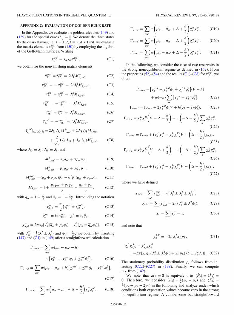
FLAVOR FLUCTUATIONS IN THREE-LEVEL QUANTUM … PHYSICAL REVIEW B 97, 235450 (2018)

APPENDIX C: EVALUATION OF GOLDEN RULE RATE

In this Appendix we evaluate the golden rule rates (149) and(139) for the special case U

V= 1. We denote the three states

by the quark flavors, i.e., l = 1,2,3 ≡ u,d,s. First, we evaluatethe matrix elements ταα′

ij from (150) by employing the algebraof the Gell-Mann matrices. Writing

ταα′ij = xαxα′ τ αα′

ij , (C1)

we obtain for the nonvanishing matrix elements

τ αα′11 = τ αα′

22 = 2J 21 M−

1,αα′ , (C2)

τ αα′12 = − τ αα′

21 = 2iJ 21 M−

2,αα′ , (C3)

τ αα′44 = τ αα′

55 = J 24 M++

3,αα′ , (C4)

τ αα′45 = − τ αα′

54 = iJ 24 M+−

3,αα′ , (C5)

τ αα′66 = τ αα′

77 = J 26 M−+

3,αα′ , (C6)

τ αα′67 = − τ αα′

76 = iJ 26 M−−

3,αα′ , (C7)

τ αα′ij |i,j∈(3,8) = 2J3iJ3jM

+1,αα′ + 2Ji8Jj8M4,αα′

+ 2√3

(J3iJj8 + Ji8J3j )M+2,αα′ , (C8)

where J33 = J3, J88 = J8, and

Mσ1,αα′ = qαqα′ + σpαpα′ , (C9)

Mσ2,αα′ =pαqα′ + σqαpα′ , (C10)

Mσσ ′3,αα′ = (qα + σpα)qα′ + σ ′qα(qα′ + σpα′ ), (C11)

M4,αα′ = 1 + pαpα′ + qαqα′

3− qα + qα′

3, (C12)

with qα = 1 + qα

3 and qα = 1 − 2qα

3 . Introducing the notation

χαα′1/3 = π

2

(ταα′

11 ± ταα′33

), (C13)

χαα′2 = iπταα′

12 , χαs = xαqα, (C14)

χαu/d = 2πxα[J 2

+(qα ± pαφz) + J 2−(pα ± qαφz)], (C15)

with J 2± = 1

2 (J 24 ± J 2

6 ) and φz = hz

h, we obtain by inserting

(147) and (C1) in (149) after a straightforward calculation

d→u =∑αα′

w(μα − μα′ − h)

× [χαα′1 − χαα′

2 φz + χαα′3 φ2

z

], (C16)

u→d =∑αα′

w(μα − μα′ + h)[χαα′

1 + χαα′2 φz + χαα′

3 φ2z

],

(C17)

s→u =∑αα′

w

(μα − μα′ − � − h

2

)χα

u χα′s , (C18)

u→s =∑αα′

w

(μα − μα′ + � + h

2

)χα

s χα′u , (C19)

s→d =∑αα′

w

(μα − μα′ − � + h

2

)χα

d χα′s , (C20)

d→s =∑αα′

w

(μα − μα′ + � − h

2

)χα

s χα′d . (C21)

In the following, we consider the case of two reservoirs inthe strong nonequilibrium regime as defined in (152). Fromthe properties (52)–(54) and the results (C1)–(C8) for ταα′

ij , weobtain

d→u = [χLR1 − χLR

2 φz + χLR3 φ2

z

](V − h)

+ w(−h)∑

α

[χαα

1 + χαα3 φ2

z

], (C22)

u→d = d→u + 2χLR2 φzV + h

(χ1 + χ3φ

2z

), (C23)

s→u = χLu χR

s

(V − � − h

2

)+ w

(−� − h

2

)∑α

χαu χα

s ,

(C24)

u→s = s→u + (χLs χR

u − χLu χR

s

)V +

(� + h

2

)χuχs,

(C25)

s→d = χLd χR

s

(V − � + h

2

)+ w

(−� + h

2

)∑α

χαd χα

s ,

(C26)

d→s = s→d + (χLs χR

d − χLd χR

s

)V +

(� − h

2

)χdχs,

(C27)

where we have defined

χ1/3 =∑αα′

χαα′1/3 = π

[J 2

1 ± J 23 ± J 2

38

], (C28)

χu/d =∑

α

χαu/d = 2π (J 2

+ ± J 2−φz), (C29)

χs =∑

α

χαs = 1, (C30)

and note that

χLR2 = −2πJ 2

1 xLpL, (C31)

χLs χR

u/d − χLu/dχ

Rs

= −2π [xLqL(J 2+ ± J 2

−φz) + xLpL(J 2− ± J 2

+φz)]. (C32)

The stationary probability distribution pl follows from in-serting (C22)–(C27) in (138). Finally, we can computemF from (142).

We note that mF = 0 is equivalent to 〈F3〉 = 〈F8〉 =0. Therefore, we consider 〈F3〉 = 1

2 (pu − pd ) and 〈F8〉 =13 (pu + pd − 2ps) in the following and analyze under whichconditions both expectation values become zero in the strongnonequilibrium regime. A cumbersome but straightforward

235450-19

LINDNER, KUGLER, SCHOELLER, AND VON DELFT PHYSICAL REVIEW B 97, 235450 (2018)

analysis yields

〈F3〉 = 1

2N[F1(s→u + s→d ) + F2(s→u − s→d )],

(C33)

2√3〈F8〉 = − 1

3N{F1[2πJ 2

+(h − 2xLpLφzV )

+ 4πJ 2−(� − xLqLV )φz + s→u − s→d ]

+ F2[2F2 + 2(d→u + u→d ) + s→u+s→d ]}.(C34)

Here, the factor N follows from the normalization condition(138). Furthermore, we have defined the following functionsin (hz,h⊥,�) space:

F1 = − 2χLR2 φzV − h

(χ1 + χ3φ

2z

)− π [J 2+(h − 2xLpLφzV )

+ 2J 2−(� − xLqLV )φz], (C35)

F2 = π [2J 2+(� − xLqLV ) + J 2

−(hz − 2plV )]. (C36)

F1 = F2 = 0 fulfills the condition 〈F3〉 = 〈F8〉 = 0. More-over, it defines a curve in (hz,h⊥,�) space that provides uswith a tool to measure the distance to the fixed-point model.

F2 = 0 directly yields (153) and defines the plane in (hz,h⊥,�)space where the curve lies in. The shape of the curve followsfromF1 = 0. To that end, we insert (153) into (C35) and obtain(154). That is, we project the curve onto the (hz,h⊥) plane.

Finally, we prove (161). To this end, we decompose (139)as

〈Iβ〉 =∑ll′

β

l′→lpl′

= Iβ

0 + Iβ

3 〈F3〉 + Iβ

8

2√3〈F8〉, (C37)

with

Iβ

0 = 1

3

∑ll′

β

l′→l , (C38)

Iβ

3 =∑

l

(

β

u→l − β

d→l

), (C39)

Iβ

8 = 1

2

∑l

(

β

u→l + β

d→l − 2β

s→l

). (C40)

Evaluating (140) for two reservoirs in the strong nonequilib-rium regime (152), we can express (C38)–(C40) in terms ofτ αα′ij :

IL0 = π

3xLxR

{[2τ LR

11 + τ LR33 + 2

(τ LR

44 + τ LR66

)+ τ LR88

]V + 2i

(τ LR

45 + τ LR67

)� + i

(2τ LR

12 + τ LR45 − τ LR

67

)hz

}, (C41)

IL3 = πxLxR

{[2iτ LR

12 + 2√3τ LR

38 + τ LR44 − τ LR

66 + i(τ LR

45 − τ LR67

)]φzV + [τ LR

44 − τ LR66 + i

(τ LR

45 − τ LR67

)]φz�

+[τ LR

11 + τ LR33 + (τ LR

11 − τ LR33

)φ2

z + 1

2

(τ LR

44 + τ LR66

)+ i

2

(τ LR

45 + τ LR67

)]h

}, (C42)

IL8 = π

2xLxR

{[2τ LR

11 + τ LR33 − (τ LR

44 + τ LR66 + τ LR

88

)+ 3i(τ LR

45 + τ LR67

)]V + [3(τ LR

44 + τ LR66

)− i(τ LR

45 + τ LR67

)]�

+[

2iτ LR12 + 3

2

(τ LR

44 − τ LR66

)− i

2

(τ LR

45 − τ LR67

)]hz

}. (C43)

If we consider mF = 0, the current Iβ is completely equal to Iβ

0 . Therefore, we can evaluate (C42) using (C2)–(C8) at the fixedpoint and obtain (161).

[1] R. Hanson, L. P. Kouwenhoven, J. R. Petta, S. Tarucha, andL. M. K. Vandersypen, Rev. Mod. Phys. 79, 1217 (2007).

[2] S. Andergassen, V. Meden, H. Schoeller, J. Splettstoesser, andM. R. Wegewijs, Nanotechnology 21, 272001 (2010).

[3] A. C. Hewson, The Kondo Problem to Heavy Fermions(Cambridge University Press, Cambridge, 1997).

[4] L. I. Glazman and M. Pustilnik, in Nanophysics: Coherence andTransport, edited by H. Bouchiat et al. (Elsevier, Amsterdam,2005), p. 427.

[5] L. I. Glazman and M. E. Raikh, Pis’ma Zh. Eksp. Teor. Fiz. 47,378 (1988) [Sov. Phys.–JETP Lett. 47, 452 (1988)]; T. K. Ngand P. A. Lee, Phys. Rev. Lett. 61, 1768 (1988).

[6] D. Goldhaber-Gordon, H. Shtrikman, D. Mahalu, D. Abusch-Magder, U. Meirav, and M. A. Kastner, Nature (London) 391,156 (1998); S. M. Cronenwett, T. H. Oosterkamp, and L. P.

Kouwenhoven, Science 281, 540 (1998); F. Simmel, R. H. Blick,J. P. Kotthaus, W. Wegscheider, and M. Bichler, Phys. Rev. Lett.83, 804 (1999).

[7] S. Sasaki, S. De Franceschi, J. M. Elzerman, W. G. van der Wiel,M. Eto, S. Tarucha, and L. P. Kouwenhoven, Nature (London)405, 764 (2000); J. Nygård, D. H. Cobden, and P. E. Lindelof,ibid. 408, 342 (2000); J. Schmid, J. Weis, K. Eberl, and K. v.Klitzing, Phys. Rev. Lett. 84, 5824 (2000); M. Eto and Yu. V.Nazarov, ibid. 85, 1306 (2000); M. Pustilnik and L. I. Glazman,ibid. 85, 2993 (2000).

[8] W. G. van der Wiel, S. De Franceschi, J. M. Elzerman, S.Tarucha, L. P. Kouwenhoven, J. Motohisa, F. Nakajima, and T.Fukui, Phys. Rev. Lett. 88, 126803 (2002); M. Pustilnik andL. I. Glazman, ibid. 87, 216601 (2001); W. Hofstetter and H.Schoeller, ibid. 88, 016803 (2001); A. Kogan, G. Granger, M. A.

235450-20

FLAVOR FLUCTUATIONS IN THREE-LEVEL QUANTUM … PHYSICAL REVIEW B 97, 235450 (2018)

Kastner, D. Goldhaber-Gordon, and H. Shtrikman, Phys. Rev. B67, 113309 (2003); W. Hofstetter and G. Zaránd, ibid. 69, 235301(2004).

[9] Y. Oreg and D. Goldhaber-Gordon, Phys. Rev. Lett. 90, 136602(2003); R. M. Potok, I. G. Rau, H. Shtrikman, Y. Oreg, andD. Goldhaber-Gordon, Nature (London) 446, 167 (2007); A. J.Keller, L. Peeters, C. P. Moca, I. Weymann, D. Mahalu, V.Umansky, G. Zaránd, and D. Goldhaber-Gordon, ibid. 526, 237(2015).

[10] L. Borda, G. Zaránd, W. Hofstetter, B. I. Halperin, and J. vonDelft, Phys. Rev. Lett. 90, 026602 (2003); S. Sasaki, S. Amaha,N. Asakawa, M. Eto, and S. Tarucha, ibid. 93, 017205 (2004);P. Jarillo-Herrero, J. Kong, H. S. J. van der Zant, C. Dekker, andL. Kouwenhoven, Nature (London) 434, 484 (2005); R. López,D. Sanchez, M. Lee, M. S. Choi, P. Simon, and K. Le Hur,Phys. Rev. B 71, 115312 (2005); M. S. Choi, R. López, and R.Aguado, Phys. Rev. Lett. 95, 067204 (2005); S. Amasha, A. J.Keller, I. G. Rau, A. Carmi, J. A. Katine, H. Shtrikman, Y. Oreg,D. and Goldhaber-Gordon, ibid. 110, 046604 (2013).

[11] A. Carmi, Y. Oreg, and M. Berkooz, Phys. Rev. Lett. 106, 106401(2011); C. Moca, A. Roman, M. Toderaş, and R. Chirla, AIPConf. Proc. 1916, 030003 (2017).

[12] C. P. Moca, A. Alex, J. von Delft, and G. Zaránd, Phys. Rev. B86, 195128 (2012).

[13] R. López, T. Rejec, J. Martinek, and R. Žitko, Phys. Rev. B 87,035135 (2013).

[14] J. König and J. Martinek, Phys. Rev. Lett. 90, 166602 (2003);M. Braun, J. König, and J. Martinek, Phys. Rev. B 70, 195345(2004); I. Weymann and J. Barnas, ibid. 75, 155308 (2007).

[15] D. Boese, W. Hofstetter, and H. Schoeller, Phys. Rev. B 64,125309 (2001); 66, 125315 (2002).

[16] V. Kashcheyevs, A. Schiller, A. Aharony, and O. Entin-Wohlman, Phys. Rev. B 75, 115313 (2007).

[17] J. Paaske, A. Andersen, and K. Flensberg, Phys. Rev. B 82,081309(R) (2010).

[18] M. Pletyukhov and D. Schuricht, Phys. Rev. B 84, 041309(2011).

[19] J. Martinek, Y. Utsumi, H. Imamura, J. Barnas, S. Maekawa,J. König, and G. Schön, Phys. Rev. Lett. 91, 127203 (2003); J.Martinek, M. Sindel, L. Borda, J. Barnas, J. König, G. Schön,and J. von Delft, ibid. 91, 247202 (2003); M. Sindel, L. Borda,J. Martinek, R. Bulla, J. König, G. Schön, S. Maekawa, and J.von Delft, Phys. Rev. B 76, 045321 (2007).

[20] Y. Meir and N. S. Wingreen, Phys. Rev. Lett. 68, 2512 (1992).[21] S. Göttel, F. Reininghaus, and H. Schoeller, Phys. Rev. B 92,

041103(R) (2015).[22] T. A. Costi, A. C. Hewson, and V. Zlatic, J. Phys.: Condens.

Matter 6, 2519 (1994).[23] A. Rosch, J. Kroha, and P. Wölfle, Phys. Rev. Lett. 87, 156802

(2001); A. Rosch, J. Paaske, J. Kroha, and P. Wölfle, ibid. 90,076804 (2003).

[24] S. Kehrein, Phys. Rev. Lett. 95, 056602 (2005); P. Fritsch andS. Kehrein, Phys. Rev. B 81, 035113 (2010).

[25] H. Schoeller, Eur. Phys. J. Special Topics 168, 179 (2009);Dynamics of open quantum systems, in Lecture Notes of the 45thIFF Spring School Computing Solids: Models, Ab initio Methodsand Supercomputing (Forschungszentrum Jülich, 2014).

[26] S. G. Jakobs, M. Pletyukhov, and H. Schoeller, Phys. Rev. B81, 195109 (2010); J. Eckel et al., New J. Phys. 12, 043042(2010).

[27] H. Schoeller and F. Reininghaus, Phys. Rev. B 80, 045117(2009); 80, 209901(E) (2009).

[28] M. Pletyukhov, D. Schuricht, and H. Schoeller, Phys. Rev. Lett.104, 106801 (2010).

[29] M. Pletyukhov and H. Schoeller, Phys. Rev. Lett. 108, 260601(2012); F. Reininghaus, M. Pletyukhov, and H. Schoeller, Phys.Rev. B 90, 085121 (2014).

[30] S. Smirnov and M. Grifoni, Phys. Rev. B 87, 121302(R) (2013);New J. Phys. 15, 073047 (2013).

[31] A. V. Kretinin, H. Shtrikman, and D. Mahalu, Phys. Rev. B 85,201301(R) (2012); O. Klochan, A. P. Micolich, A. R. Hamilton,D. Reuter, A. D. Wieck, F. Reininghaus, M. Pletyukhov, and H.Schoeller, ibid. 87, 201104(R) (2013).

[32] F. B. Anders and A. Schiller, Phys. Rev. Lett. 95, 196801 (2005);F. B. Anders, R. Bulla, and M. Vojta, ibid. 98, 210402 (2007);A. Hackl, D. Roosen, S. Kehrein, and W. Hofstetter, ibid. 102,219902(E) (2009).

[33] A. J. Daley, C. Kollath, U. Schollwoeck, and G. Vidal, J. Stat.Mech.: Theory Exp. (2004) P04005; S. R. White and A. E.Feiguin, Phys. Rev. Lett. 93, 076401 (2004); P. Schmitteckert,Phys. Rev. B 70, 121302 (2004); F. Heidrich-Meisner, A. E.Feiguin, and E. Dagotto, ibid. 79, 235336 (2009).

[34] S. Weiss, J. Eckel, M. Thorwart, and R. Egger, Phys. Rev. B 77,195316 (2008).

[35] T. L. Schmidt, P. Werner, L. Mühlbacher, and A. Komnik, Phys.Rev. B 78, 235110 (2008).

[36] F. Schwarz, I. Weymann, J. von Delft, and A. Weichselbaum,arXiv:1708.06315.

[37] C. Caroli, R. Combescot, P. Nozières, and D. Saint-James,J. Phys. C: Solid State Phys. 4, 916 (1971); 5, 21 (1972).

[38] S. Coleman, Aspects of Symmetry, 1st ed. (Cambridge UniversityPress, Cambridge, 1985); H. Georgi, Lie Algebras in ParticlePhysics: From Isospin to Unified Theories, 2nd ed., Frontiers inPhysics, Vol. 54 (Westview, Boulder, CO, 1999).

[39] D. Griffiths, Introduction to Elementary Particles, 2nd ed.(Wiley, Weinheim, 2008).

[40] R. Bulla, T. A. Costi, and T. Pruschke, Rev. Mod. Phys. 80, 395(2008).

[41] A. Weichselbaum and J. von Delft, Phys. Rev. Lett. 99,076402 (2007); A. Weichselbaum, Phys. Rev. B 86, 245124(2012).

[42] A. Weichselbaum, Ann. Phys. 327, 2972 (2012).

235450-21