leopold{franzens{universit at innsbruck semantic technologies institute (sti) innsbruck submitted to...
TRANSCRIPT

Leopold–Franzens–Universitat
Innsbruck
Semantic Technologies Institute (STI)
Innsbruck
Submitted to the Faculty of Mathematics, Computer
Science and Physics of the University of Innsbruck
In partial fulfillment of the requirements
for the degree of Master of Science
RIF4J - A Reasoning Engine for RIF-BLD
Supervisors
Dr. Reto Krummenacher
Dr. Katharina Siorpaes
Univ.-Prof. Dr. Dieter Fensel
Handed in by
Adrian Marte
Innsbruck, March 23, 2011

Abstract
Logic programming is a formalism, which provides means for the formal representa-
tion of knowledge in the form of rules. With rules, knowledge can be represented in a
way that facilitates efficient reasoning upon the knowledge, in order to, for instance,
derive new knowledge from existing one. There exist various logic programming
languages, often also referred to as rule languages, and extensions thereof, each hav-
ing different features with respect to syntax and semantics. One such language is
Datalog, which aims at combining the logic programming paradigm with relational
databases.
As there is not only a variety of rule languages, but also of systems that provide sup-
port for those languages, the need arises for a format that allows the interchange of
rules between heterogeneous systems. The Rule Interchange Format (RIF) is a W3C
Recommendation that aims at specifying a format that can be used for knowledge
exchange between various rule systems based on a common syntax. Particularly
important with respect to rule-based reasoning are the profiles that RIF defines.
Profiles reflect particular use case requirements and yield purposeful balances be-
tween expressivity and computational complexity. For instance, the Basic Logic
Dialect (RIF-BLD) is a RIF profile that is designed to have limited expressiveness
and reasoning characteristics that allow the exchange of rules between a large set of
existing logic programming systems.
This thesis presents the design and implementation of RIF4J, a reasoning engine
that allows for the programmatic processing of knowledge represented in the Basic
Logic Dialect (BLD) of RIF, and enables the reasoning upon this knowledge using
the Datalog system IRIS. This is realized through a translation of RIF-BLD formulas
to equivalent Datalog programs. As RIF is intended for being applied to the Web
where the amount of data is extremely large, IRIS-RDB is developed as an extension
of IRIS that leverages the close relationship of Datalog and relational algebra in order
to take advantage of a relational database system to process data that exceeds the
limits of a single computer’s memory.
I

Submitted Papers
While working on this thesis the following papers have been submitted:
• Reto Krummenacher, Daniel Winkler and Adrian Marte. WSML2Reasoner -
A Comprehensive Reasoning Framework for the Semantic Web. International
Semantic Web Conference 2010 Posters and Demonstrations Track: Collected
Abstracts. November 2010.
• Daniel Winkler, Reto Krummenacher and Adrian Marte. RIF-BLD Reasoning
with IRIS. RuleML-2010 Challenge. October 2010.
• Adrian Marte. D3.2.8 Enhanced Reasoning Framework Core. EU FP7 SOA4All
project deliverable. February 2011.
• Florian Fischer, Ioan Toma, Valer Roman, Adrian Marte and Iker Larizgoitia.
D4.4.2 Implementation of Rule-based Reasoning Plug-in. EU FP7 LarKC
project deliverable. March 2011.
Declaration
The work presented here was undertaken within the Department of Computer Sci-
ence at the University of Innsbruck. I confirm that no part of this work has pre-
viously been submitted for a degree at this or any other institution and, unless
otherwise stated, it is the original work of the author.
Adrian Marte, March 2011
II

Acknowledgment
I would like to express my appreciation and gratitude to the people who provided
invaluable assistance in the development and completion of this thesis. First, I would
like to thank my supervisors Dr. Reto Krummenacher, Dr. Katharina Siorpaes and
Univ.-Prof. Dr. Dieter Fensel for their support and supervision. Special thanks go
to Dr. Reto Krummenacher for the helpful suggestions and his commitment during
the work on this thesis.
I am also very grateful to my friends Daniel, Gigi, Fritz, Stefan, Rafael, Jurgen,
William, Martin, Gregor, Thomas and everybody I forgot to mention, for the great
time during the studies that I will never forget in my life. I am especially grateful
to Daniel Winkler without whom this thesis would not have been possible.
Further, I would like to thank my girlfriend for her understanding, patience and
support in the past years. My deepest gratitude goes to my family for their support
and for just believing in me throughout my life.
III

Contents
1. Introduction 1
1.1. Research Question . . . . . . . . . . . . . . . . . . . . . . . . . . . . 3
1.2. Contribution . . . . . . . . . . . . . . . . . . . . . . . . . . . . . . . . 4
1.3. Structure . . . . . . . . . . . . . . . . . . . . . . . . . . . . . . . . . 5
2. Background 7
2.1. Logic Programming . . . . . . . . . . . . . . . . . . . . . . . . . . . . 7
2.1.1. Syntax of General Logic Programs . . . . . . . . . . . . . . . 8
2.1.2. Semantics of General Logic Programs . . . . . . . . . . . . . . 9
2.1.3. Representing Knowledge in General Logic Programs . . . . . . 13
2.1.4. Answering Queries . . . . . . . . . . . . . . . . . . . . . . . . 15
2.2. Datalog . . . . . . . . . . . . . . . . . . . . . . . . . . . . . . . . . . 16
2.2.1. Syntax of Datalog Programs . . . . . . . . . . . . . . . . . . . 16
2.2.2. Datalog and Relational Databases . . . . . . . . . . . . . . . . 17
2.2.3. Semantics of Datalog Programs . . . . . . . . . . . . . . . . . 20
2.2.4. Computing the Least Herbrand Model . . . . . . . . . . . . . 21
2.2.5. Extension of Pure Datalog . . . . . . . . . . . . . . . . . . . . 27
2.3. Rule Interchange Format . . . . . . . . . . . . . . . . . . . . . . . . . 29
2.3.1. Overview . . . . . . . . . . . . . . . . . . . . . . . . . . . . . 30
2.3.2. Basic Logic Dialect . . . . . . . . . . . . . . . . . . . . . . . . 31
3. RIF4J 52
3.1. Overview . . . . . . . . . . . . . . . . . . . . . . . . . . . . . . . . . . 52
3.2. Object Model . . . . . . . . . . . . . . . . . . . . . . . . . . . . . . . 53
3.2.1. Mutability . . . . . . . . . . . . . . . . . . . . . . . . . . . . . 54
IV

Contents
3.2.2. Visitor Pattern . . . . . . . . . . . . . . . . . . . . . . . . . . 54
3.3. XML Parser . . . . . . . . . . . . . . . . . . . . . . . . . . . . . . . . 56
3.4. Serializers . . . . . . . . . . . . . . . . . . . . . . . . . . . . . . . . . 57
3.5. Reasoning with Datalog . . . . . . . . . . . . . . . . . . . . . . . . . 57
3.6. Mapping RIF-BLD to Datalog . . . . . . . . . . . . . . . . . . . . . . 59
3.6.1. Transformations . . . . . . . . . . . . . . . . . . . . . . . . . . 59
3.6.2. RIF-BLD Semantics Through Meta-Level Axioms . . . . . . . 64
3.6.3. Logical Entailment Checking with Datalog Queries . . . . . . 65
4. IRIS-RDB 67
4.1. IRIS . . . . . . . . . . . . . . . . . . . . . . . . . . . . . . . . . . . . 67
4.2. Problems with IRIS . . . . . . . . . . . . . . . . . . . . . . . . . . . . 68
4.3. Features of IRIS and IRIS-RDB . . . . . . . . . . . . . . . . . . . . . 68
4.3.1. Supported Datatypes . . . . . . . . . . . . . . . . . . . . . . . 69
4.3.2. Built-in Predicates . . . . . . . . . . . . . . . . . . . . . . . . 70
4.3.3. Rule Head Equality . . . . . . . . . . . . . . . . . . . . . . . . 70
4.4. Rule Evaluation Process . . . . . . . . . . . . . . . . . . . . . . . . . 70
4.4.1. Program Optimization . . . . . . . . . . . . . . . . . . . . . . 71
4.4.2. Rule Safety Processing . . . . . . . . . . . . . . . . . . . . . . 72
4.4.3. Stratification . . . . . . . . . . . . . . . . . . . . . . . . . . . 72
4.4.4. Rule Re-Ordering . . . . . . . . . . . . . . . . . . . . . . . . . 73
4.4.5. Rule Optimization . . . . . . . . . . . . . . . . . . . . . . . . 74
4.4.6. Rule Compilation . . . . . . . . . . . . . . . . . . . . . . . . . 75
4.4.7. Rule Evaluation . . . . . . . . . . . . . . . . . . . . . . . . . . 76
4.5. Translation of Datalog Programs into Relation Algebra . . . . . . . . 76
4.5.1. The Relation of a Predicate . . . . . . . . . . . . . . . . . . . 76
4.5.2. The Relation Defined By a Rule Body . . . . . . . . . . . . . 78
4.5.3. The Relational Views for a Rule . . . . . . . . . . . . . . . . . 81
5. Evaluation 83
5.1. RIF4J . . . . . . . . . . . . . . . . . . . . . . . . . . . . . . . . . . . 83
5.1.1. Positive Entailment Test . . . . . . . . . . . . . . . . . . . . . 84
5.1.2. Negative Entailment Test . . . . . . . . . . . . . . . . . . . . 87
5.1.3. Evaluation Conclusion . . . . . . . . . . . . . . . . . . . . . . 88
5.2. IRIS-RDB . . . . . . . . . . . . . . . . . . . . . . . . . . . . . . . . . 88
5.2.1. OpenRuleBench . . . . . . . . . . . . . . . . . . . . . . . . . . 89
5.2.2. Evaluation Conclusion . . . . . . . . . . . . . . . . . . . . . . 93
V

Contents
6. Conclusion 95
6.1. Contribution . . . . . . . . . . . . . . . . . . . . . . . . . . . . . . . . 95
6.2. Future Work . . . . . . . . . . . . . . . . . . . . . . . . . . . . . . . . 96
A. Algorithms 98
B. Installation and Configuration 101
B.1. RIF4J . . . . . . . . . . . . . . . . . . . . . . . . . . . . . . . . . . . 101
B.1.1. Installation . . . . . . . . . . . . . . . . . . . . . . . . . . . . 101
B.1.2. Usage Example . . . . . . . . . . . . . . . . . . . . . . . . . . 102
B.2. IRIS-RDB . . . . . . . . . . . . . . . . . . . . . . . . . . . . . . . . . 103
B.2.1. Installation . . . . . . . . . . . . . . . . . . . . . . . . . . . . 103
B.2.2. Configuration . . . . . . . . . . . . . . . . . . . . . . . . . . . 104
B.2.3. Usage Example . . . . . . . . . . . . . . . . . . . . . . . . . . 105
List of Tables 108
List of Listings 109
List of Figures 110
Bibliography 111
VI
1
Introduction
The World Wide Web consists of billions of Web pages, information that is mainly
designed and intended for humans. In most cases this data is represented in a form
that is easy to produce and consume by a human user of the World Wide Web. With
techniques, such as HTTP, HTML and URI, it is not only possible to present data,
but also to interlink such Web pages, a mechanism for which the Web is famous
for, and which is also one of the foundations for its success. For humans it is easy
to understand the information available on the Web, to transform it into different
representations or to put the data into relation with each other. However, this often
unstructured data and the heterogeneity of the information and the technologies
involved in the presentation of such, makes it difficult for machines to process the
information.
Although current search engines, such as Google1 or Bing2, already do an excellent
job in finding, integrating and representing information on the Web by using intelli-
gent algorithms and techniques, they are often limited to discovering certain strings
appearing on the Web disregarding the semantics they may carry. This makes it
hard to find the relevant information in today’s abundance of data on the Web. For
instance, when a user searches for information about “dog” he may also expect to
find data about “dachshund”. As the search engine may only respect information
containing the keyword “dog” or “dogs”, it may disregard any data referring to a
“dachshund” since the system does not know that a “dachshund” is also a dog.
The Semantic Web represents an extension of the World Wide Web and has the goal
to give meaning to the data published in the Web, such that also machines, and not
1Google, http://www.google.com [last checked 12.03.2011]2Bing, http://www.bing.com [last checked 12.03.2011]
1

Chapter 1. Introduction
only humans, can understand and automatically and intelligently process the data
and the relationships between them. Recently, the term Linked Data emerged as
a paradigm for publishing and interlinking data – rather than Web pages – that
enables to take advantage of Semantic Web technologies and makes it possible to
automatically access, analyze and process the abundance of information available
on the Web. The adaption of this approach gains considerable popularity in various
areas of industry, science and public administrations, which leads to a continuous
growth of data published following the Linked Data principles.3
Formal languages are used to describe and annotate the data, in order to allow
machines to interpret it and reason about it, i.e., to check consistency, to answer
queries, or to infer new otherwise uncovered knowledge. In response to the im-
mense amount of data, formalisms are sought that allow for tractable and efficient
reasoning algorithms. The difficulty with such languages is the trade-off between
the requirements for expressivity and the usefulness for enabling tractable reasoning
characteristics.
Logic programming (Section 2.1) is a formalism, which provides means for the formal
representation of knowledge in the form of rules. With rules knowledge can be
represented in a way that facilitates efficient reasoning upon the knowledge, in order
to, for instance, derive new knowledge from existing one. There exist various logic
programming languages (often also referred to as rule languages) and extensions
thereof, each having different features with respect to syntax and semantics. One
such language is Datalog (Section 2.2), which aims at combining logic programming
with relational databases. As there is not only a variety of rule languages, but also
of systems that provide support for those languages, the need arises for a format
that allows the interchange of rules between heterogeneous systems.
The Rule Interchange Format (RIF) (Section 2.3) is a W3C Recommendation that
aims at specifying a format that can be used for knowledge exchange between various
rule systems based on a common syntax. Particularly important with respect to
rule-based reasoning are the semantic profiles that RIF defines. Profiles reflect
particular use case requirements and yield purposeful balances between expressivity
and computational complexity. For instance, the Basic Logic Dialect (RIF-BLD) is
a RIF profile that allows logic rules to be exchanged between rule-based systems.
The support for different profiles is not only reflected in RIF, but also in another
recent standard by the W3C. The updated Web Ontology Language standard OWL
3Linked Data principles, http://www.w3.org/DesignIssues/LinkedData.html [lastchecked 22.03.2011]
2

Chapter 1. Introduction
2 [20] provides dialects that are restricted in their semantic expressivity for the sake
of better reasoning behavior; e.g., the OWL-RL profile is intended to be amenable
to implementations using rule-based technologies. The very same idea is at the basis
of the WSML [13] language family, where the variants WSML-Flight and WSML-
Rule restrict their expressivity in order to enable rule-based reasoning. Defining
such language variants helps in establishing formalisms that are expressive enough
to be useful, while exhibiting reasoning characteristics that can also scale to the size
of the Web. In the context of Linked Data the trade-off between expressivity and
scalability is particularly important when considering the abundance of data and
the additional knowledge that may possibly be derived from it, depending on the
formalism and the implied computational complexity.
1.1. Research Question
Various systems have been implemented over the last years that allow for reason-
ing using rule-based formalism. One such system is the open-source, Java-based
Datalog reasoner IRIS, which has been continuously extended in the course of the
integrated project SOA4All4. IRIS can be used as core engine for different rea-
soners that tackle diverse formalism ranging across various OWL 2 and WSML
dialects. Effectively, IRIS is applied in different research projects for diverse tasks,
e.g., semantic discovery, ranking and design-time service composition in the inte-
grated project SOA4All or as general purpose rule-based reasoning plug-in in the
integrated project LarKC5.
This thesis addresses the challenge of designing and implementing a RIF-BLD con-
formant reasoning engine based on a Datalog system in general, and IRIS in partic-
ular. This leads directly to the main research question of this thesis.
Main Question: How can RIF-BLD reasoning tasks be accomplished with a
Datalog engine?
In order to better structure the scientific and technological challenges, the main
research question is divided into three sub-questions. The first question refers to
the goal of encoding knowledge represented as RIF-BLD formulas in a Java object
model enabling the programmatic processing of the knowledge. This facilitates the
4SOA4All, http://www.soa4all.eu [last checked 09.03.2011]5LarKC - Large Knowledge Collider, http://www.larkc.eu/ [last checked 09.03.2011]
3

Chapter 1. Introduction
implementation of algorithms on top of the object model to improve flexibility and
extendability of the software component.
Question 1: How to design an object model which allows for the programmatic
processing of RIF-BLD formulas?
Given an object model for RIF-BLD, a Java implementation should be developed
that takes advantage of the Datalog reasoner IRIS for carrying out RIF-BLD rea-
soning tasks. Hence, the second question concerns the semantics-preserving trans-
formations of RIF-BLD formulas to the Datalog language supported by IRIS, which
enables RIF-BLD reasoning using the formalism of Datalog.
Question 2: How to transform RIF-BLD into Datalog programs preserving the
semantics of RIF?
In IRIS the evaluation of Datalog programs is only handled in memory. As RIF es-
pecially targets application to the Web where the amount of data is extremely large,
the system needs to be extended in order to be able to process data that exceeds
the limits of a single computer’s memory, which leads to the third question.
Question 3: How to build a more scalable Datalog system?
In summary, the main goal of this thesis is to investigate how to build a RIF-BLD
reasoning engine based on the Datalog reasoner IRIS. Furthermore, the current
limitations of the in-memory implementation of IRIS shall be overcome to have a
more scalable Datalog system cable of handling large amounts of data.
1.2. Contribution
The contribution of this thesis is to design and implement a reasoning engine, re-
ferred to as RIF4J, that allows for the programmatic processing of knowledge rep-
resented in the Basic Logic Dialect (BLD) of RIF, and enables the reasoning upon
this knowledge using the Datalog system IRIS. This is realized through a trans-
lation of RIF-BLD formulas to equivalent Datalog programs. In order to support
data that exceeds the limits of a single computer’s memory, IRIS-RDB is developed
4

Chapter 1. Introduction
as an extension of IRIS that leverages the close relationship of Datalog and rela-
tional algebra, and implements an evaluation strategy based on a relational database
system.
More concretely, the contribution of this thesis is threefold, matching the three
research sub-questions discussed above:
RIF4J provides an object model capable of representing RIF-BLD formulas in the
Java programming language. The system is designed with flexibility and ex-
tendability in mind encouraging the implementation of additional algorithms
and utilities on top of RIF4J. Examples of additional features are the inte-
grated utilities for parsing and serializing RIF-BLD formulas.
RIF-BLD reasoning with Datalog is realized by a semantic-preserving transla-
tion from RIF-BLD to Datalog such that the resulting Datalog programs and
queries can be evaluated using a Datalog engine. A formal definition of this
translation is specified and an implementation thereof is provided based on the
RIF4J and IRIS object models. Two prototype implementations of RIF-BLD
reasoners based on the Datalog engines IRIS and IRIS-RDB are provided,
where both systems take advantage of the translation implementation in order
to carry out RIF-BLD reasoning tasks.
IRIS-RDB is an extension of IRIS that uses a relational database as an underlying
system to evaluate Datalog programs. The goal of IRIS-RDB is to have a more
scalable reasoning engine that is able to process knowledge bases that exceed
the limits of a single computer’s memory.
1.3. Structure
Chapter 2 gives an introduction to the field of logic programming. The first section
reviews general logic programming, a common subset that enables the formulation of
simple logic programs. In the second section, a simplified version of logic program-
ming, called Datalog, is outlined. The third section gives an introduction to the Rule
Interchange Format (RIF) with a more detailed overview of the Basic Logic Dialect
(BLD), a format that allows logic rules to be exchanged between rule systems.
Chapter 3 describes RIF4J, a reasoning engine for RIF-BLD that provides a Java
object model and two prototype implementations of RIF-BLD reasoners based on
the Datalog engines IRIS and IRIS-RDB. The chapter also gives the definition of
5
Chapter 1. Introduction
the necessary transformation from RIF-BLD to Datalog and shows the syntactic
and semantic correspondence of the two languages.
Chapter 4 continues with a description of IRIS-RDB, an extension of the Datalog
reasoner IRIS that uses a relational database as an underlying system to evaluate
Datalog programs.
Chapter 5 presents the results of the evaluation of the software components devel-
oped in the course of this master thesis. For RIF4J the RIF-BLD conformance of the
two prototype reasoners is evaluated, while the evaluation of IRIS-RDB focuses on
the comparison of the original IRIS with IRIS-RDB with respect to the performance
and scalability of the system.
Chapter 6 concludes this master thesis with a recapitulation of the established con-
tributions and gives an outlook to further research topics in the area.
6

2
Background
This chapter gives an overview of logic programming, Datalog and the Rule Inter-
change Format (RIF). Logic programming languages, often called rule languages,
provide means to represent knowledge in the form of rules, which allow for the
derivation of new knowledge from existing one and, more importantly, the reasoning
over this knowledge. Datalog is a simplified version of logic programming, which
is designed for reasoning over large knowledge bases usually stored in a relational
database. The Rule Interchange Format is a W3C recommendation for the exchange
of rules defined using different rule languages among heterogeneous systems without
changing the meaning of the rules. A summary of the the most important aspects
of these formalisms will be given, which explains the inclusion of large parts of the
respective literature. This chapter does not contain any new mathematical results.
2.1. Logic Programming
Over the past decades, various dialects and extensions for logic programming have
been defined and developed [4]. This section outlines a common subset that enables
the formulation of simple logic programs, which in the literature are also referred to
as general logic programs. We restrict ourselves to this language as it is sufficient for
the understanding of the concepts of Datalog and the Rule Interchange Format.
7

Chapter 2. Background
2.1.1. Syntax of General Logic Programs
A general logic program [4] consists of a finite set of rules. Rules are sentences which
allow to deduce new knowledge from existing one, such as: “If X is a parent of Y
and if Y is a parent of Z, the X is the grandparent of Z”. More formally, rules are
expressions of the form
A0 ← A1, . . . , Am, not Am+1, . . . , not An (1)
which is a notational variant of the formula
(A1 ∧ . . . ∧ Am ∧ not Am+1 ∧ . . . ∧ not An)→ A0
where the Ai’s are atoms of the form p(t1, . . . , tm), where the t’s are terms and p is
a predicate symbol of arity m. A term is either a constant, a variable or a function
symbol with terms as arguments. The symbol not denotes the logical connective
called negation as failure [12], which captures what is believed or assumed to be
false (closed-world assumption).6 General logic programs that do not have not and,
therefore, do not support negation as failure are called definite programs. The left-
hand side of a rule is called its head and the right-hand side is called its body. A
rule of the form A←, i.e., a rule with an empty body, is called fact. Formulas and
rules that do not contain variables are called ground. In the following, we use strings
beginning with a lower-case character for constants, functions and predicates and
strings beginning with an upper-case character for variables. A set of rules together
with a set of facts is often also called knowledge base.
For example, the rule “If X is a parent of Y and if Y is a parent of Z, then X is the
grandparent of Z” can be represented in general logic programming as
grandparent(X,Z)← parent(X, Y ), parent(Y, Z)
Here the symbols grandparent and parent are predicate symbols, the symbols X,
Y and Z are variables, grandparent(X,Z), parent(X, Y ), and parent(Y, Z) are
atoms.
6The closed-world assumption is the presumption that what is not currently known to be true, isconsidered to be false.
8
Chapter 2. Background
2.1.2. Semantics of General Logic Programs
The Herbrand universe H(Π) of a program Π is the set of ground terms, i.e., all
terms except variables, that use the function symbols and constants that appear in
the program. The Herbrand base HB(Π) is the set of all ground atoms formed by
predicate symbols in the program whose arguments are in the Herbrand universe
H(Π). If the program contains a function symbol of positive arity, then the Herbrand
universe and Herbrand base are countably infinite, otherwise, they are finite [38,
page 624].
The set atoms(p) will denote the subset of HB(Π) formed with a predicate p, i.e.
all ground terms with predicate p. For a set of predicates A, atoms(A) will denote
the subset of HB(Π) formed with the predicates in A. Unless otherwise stated,
atoms in the Herbrand base and ground rules are considered whose variables have
been instantiated to elements of the Herbrand universe, which are called instantiated
rules [38, page 624]. Furthermore, it is assumed that all rules containing variables
are used as shorthand for the respective instantiated rules.
Definition 2.1.1. (Reproduced from [38, page 624]) The Herbrand instantiation
of a general logic program is the set of rules obtained by substituting terms in the
Herbrand universe for variables in every possible (coherent) way. An instantiated
rule is one in the Herbrand instantiation. Whereas “uninstantiated” logic programs
are assumed to be a finite set of rules, instantiated logic programs may well be
infinite.
The semantics of a general logic program are given by its stable models, which are
defined as follows:
Definition 2.1.2. (Reproduced from [4, page 5]) The stable model of a definite
program Π is the smallest subset S ofHB(Π) such that for any ruleA0 ← A1, . . . , Am
from Π, if A1, . . . , Am ∈ S, then A0 ∈ S. In the following, a(Π) will denote the stable
model of a definite program Π, i.e., a program without rules containing a not. Let
Π be an arbitrary general logic program Π. For any set S of atoms, let ΠS be a
program obtained from Π by deleting
1. Each rule that has a formula not A in its body with A ∈ S, and
2. All formulas of the form not A in the bodies of the remaining rules.
In this step, all not occurring in Π are removed. Therefore, ΠS is a definite program,
for which the stable model is already defined. If this stable model coincides with S,
9

Chapter 2. Background
then S is a stable model of Π. In other words, a stable model of Π is characterized
by the equation
S = a(ΠS).
2.1.2.1. Querying General Logic Programs
The possibility to check if a specific general logic program fulfills certain properties
is an important aspect in logic programming. In general, this is realized by posing
a query in the form of a formula to a logic program and check if the program entails
this formula, formally defined in the following.
A ground atom P is true in S if P ∈ S, otherwise P is false (i.e. ¬P is true) in
S. The definition is extended to arbitrary first-order formulas in a standard way [4,
page 6]. Π entails a formula f , written as Π |= f if f is true in all stable models of
Π. The answer to a ground query q is yes if q is true in all stable models of Π, no
if ¬q is true in all stable models of Π and unknown otherwise.
Example 2.1.1. ([4, page 6]) Consider the general logic program
Π = {p(X)← not q(X), q(a)←}
Let us show that a set S = {q(a), p(b)} is a stable model Π. According to Definition
2.1.2, ΠS = {p(b) ←, q(a) ←} whose stable model is equal to S. Therefore, S is a
stable model of Π.
2.1.2.2. Non-Monotonicity
General logic programs with negation as failures (not) are non-monotonic, i.e. adding
new facts to the program may cause the withdrawal of previously derived facts. Con-
sider, for instance, if we would add the fact q(b)← to the program in Example 2.1.1,
then the new program would not entail p(b), although the old program did.
2.1.2.3. Categorical, Incoherent and Coherent Logic Programs
Uniqueness of a stable model is an important property of a logic program. Programs
that have a unique stable model are called categorical. However, there are programs,
which have multiple stable models or no stable models at all. The former are called
coherent, while the latter are called incoherent [4, page 6]. Example 2.1.2 shows
10

Chapter 2. Background
an incoherent program and Example 2.1.3 shows a coherent, but not categorical
program.
Example 2.1.2. ([4, page 6f]) Consider the general logic program
Π = {p← not p}
Assume that Π has a stable model S. We can now show that the program is
incoherent by showing a contradiction considering the following two cases:
1. If p ∈ S then ΠS is empty and so its stable model. Since S is not empty it is
not a stable model of Π
2. If p 6∈ S then ΠS = {p ←}, whose stable model is T = {p}. As p ∈ T but
p 6∈ S, S is not a stable model of Π.
The contradiction falsifies our assumption and, therefore, Π has no stable model
and Π is incoherent.
Example 2.1.3. ([4, page 7]) Consider the general logic program
Π = {p← not q, q ← not p}
Assume that p ∈ S then ΠS = {q ←}, whose stable model is {q}. Now assume that
q ∈ S then ΠS = {p←} and its stable model is {p}. Clearly, the program hast two
stable models and is, therefore, coherent but not categorical.
2.1.2.4. Stratification
Coherence and categoricity are important properties of logic programs, as such pro-
grams, in turn, have important properties, some of which are shown in the follow-
ing.
Definition 2.1.3. (Reproduced from [4, page 7]) A partition π0, . . . , πk of the set
of all predicate symbols of a general logic program Π is a stratification of Π, if for
any rule of the type (1)7 and for any p ∈ πs, 0 ≤ s ≤ k if A0 ∈ atoms(p), then:
1. For every 1 ≤ i ≤ m there is a q and j ≤ s such that q ∈ πj and Ai ∈ atoms(q)
2. For every m + 1 ≤ i ≤ n there is a q and j < s such that q ∈ πj and
Aj ∈ atoms(q).7See beginning of Section 2.1.1
11

Chapter 2. Background
In other words, π0, . . . , πk is a stratification of Π if for all rules in Π, the predicates
that appear only positively in the body of a rule are in a stratum lower than or
equal to the stratum of the predicate in the head of the rule, and the predicates
that appear under negation as failure are in a strata lower than the stratum of the
predicate in the head of the rule.
Given stratified predicates the rules can also be grouped into strata by assigning
rule r to stratum πi, where πi is the stratum assigned to the head predicate of r. A
program that has a stratification is called a stratified program.
Example 2.1.4. ([4, page 7]) Consider a general logic program Π consisting of rules
1. p(f(X)) ← p(X), not q(X)
2. p(a) ←
3. q(X) ← not r(X)
4. r(a) ←
Π is stratified with a stratification {r}, {q}, {p}. q is in a higher stratum as r, since,
according to rule 3, q has a negative dependency on r. Analog, p is in a higher
stratum than q, as, according to rule 1, p has a negative dependency on q.
For the following definitions the concept of a dependency graph is required. A de-
pendency graph identifies how predicates in a logic program depend on one another,
which eases the process of checking if a logic program is stratified or not. The de-
pendency graph DΠ of a program Π consists of the predicate names as the vertices
of the graph. There is a labeld edge < Pi, Pj, s > in DΠ iff there is a rule r in Π
with Pi in its head and Pj in its body and the label s ∈ {+,−} denotes whether Pj
appears in a positive or a negative literal in the body of r. Note that an edge may
be labeled both with + and −. A negative cycle in the dependency graph is a cycle
that contains at least one edge with a negative label [4, page 8].
Proposition 2.1.1. (Reproduced from [4, page 8][31]) A general logic program Π
is stratified iff its dependency graph DΠ does not contain any negative cycles.
Proposition 2.1.2. (Reproduced from [4, page 8][31][18]) Any stratified general
logic program is categorical and has a unique stable model.
The program in Example 2.1.4 is stratified and, therefore, is a categorical program
having exactly one stable model. For further sections, the following Lemma about
general logic programs is required.
12
Chapter 2. Background
Lemma 2.1.1. (Reproduced from [4, page 8]) For any stable model S of a general
logic program Π:
(a) For any ground instance of a rule of the type (1) from Π,
if {A1, . . . , Am} ⊆ S and {Am+1, . . . , An} ∩ S = ∅ then A0 ∈ S.
(b) If A0 ∈ S, then there exists a ground instance of a rule of type (1) from Π
such that {A1, . . . , Am} ⊆ S and {Am+1, . . . , An} ∩ S = ∅.
2.1.3. Representing Knowledge in General Logic Programs
This section gives an overview of knowledge representation using general logic pro-
gramming and show how to reason upon this knowledge using the formalisms and
methods defined so far. The example used in this section has been taken from [4,
page 8ff].
Consider the following knowledge about birds: birds typically fly and penguins are
non-flying birds. We also know that Tweety is a bird. Suppose now, that we want
to build a cage for Tweety and we want to know if we also need to put a roof on it,
in order to avoid that Tweety flies away. For this, we need to find out, if Tweety is
actually able to fly. Example 2.1.5 shows how this knowledge can be represented by
a general logic program.
Example 2.1.5. ([4, page 9]) Consider a general logic program B consisting of rules
and facts about particular birds
1. f lies(X)← bird(X), not ab(r1, X)
2. bird(X)← penguin(X)
3. ab(r1, X)← penguin(X)
4. make top(X)← flies(X)
and facts about two particular birds
f1. bird(tweety)←
f2. penguin(sam)←
Rule 1 captures the knowledge that birds can usually fly, although some exception
may exist. r1 is a constant used to name rule 1 and the atom ab(r1, X) denotes birds
that are not able to fly. Statements of this form are often called default assumptions
or just defaults. Rule 2 expresses the knowledge that penguins are birds. With rule
13

Chapter 2. Background
3 we express that penguins cannot fly. Such rules are sometimes called cancellation
rules, as they block the application of a rule. In our case rule 3 may block the
application of rule 1. Finally, rule 4 determines if we have to put a top on our cage
or not.
Rule 1 expresses a normative statement about the flying ability of birds. In gen-
eral, normative statements are of the form “A’s are normally B’s” and are usually
represented by general logic program rules
b(X)← a(X), not ab(r,X)
where r is a constant used to name the rule. Exceptions to normative statements of
the form “C’s are exceptional A’s. They are not B’s” are expressed with a rule
ab(r,X)← c(X)
Such rules are often referred to as strong exceptions.
The general logic program B shown in Example 2.1.5 is stratified and, thus, has
a unique stable model, see Definition 2.1.2. A stratification of the program is
{penguin}, {ab, bird}, {flies}, {make top}. Lemma 2.1.1 can now be used to find
out if the two birds Tweety and Sam can fly by posing two queries flies(tweety)
and flies(sam) to the logic program B.
Assume, we want to check if Tweety can fly, therefore, we need to check if the answer
to the query flies(tweety) is yes. Let S be the stable model of B. According to
Lemma 2.1.1, flies(tweety) ∈ S iff
1. bird(tweety) ∈ S and
2. ab(r1, tweety) 6∈ S.
Statement 1 follows from fact f1 and the lemma. To show statement 2, we need to
show that penguin(tweety) 6∈ S, which also follows from the lemma. As we have
proved statement 1 and 2, we can now use rule 1 and (a) from the lemma to show
flies(tweety) ∈ S and, thus, the answer to the query flies(tweety) is yes.
In a similar way, we now find the answer to the query flies(sam). Again, let S be
the stable model of B. According to Lemma 2.1.1, flies(sam) ∈ S iff
1. bird(sam) ∈ S and
14

Chapter 2. Background
2. ab(r1, sam) 6∈ S.
To show statement 1, we need to show that penguin(sam) ∈ S, which follows
from the fact f2 and the lemma.8 To show statement 2, we need to show that
penguin(sam) 6∈ S, which is, however, not the case as according to the fact f2
penguin(sam) ∈ S. According to rule 1 and the lemma, flies(sam) 6∈ S and,
therefore, the answer to the query flies(sam) is no.
2.1.4. Answering Queries
The above example is a typical example of reasoning with inheritance hierarchies,
where the hierarchies consist of entities that share some properties. The example
from above expresses that birds can usually fly but there exist exceptions to this
assumption. For instance, it has been formalized, that penguins, although they are
birds, are not able to fly. Using the formalism of logic programming this knowledge
has been expressed using rules and facts. Finally, queries have been utilized in order
to check if the two objects Tweety and Sam have the ability to fly and, thus, it has
been reasoned about the knowledge captured by the logic program.
In the literature, various methods have been suggested to compute the answers to
queries with respect to logic programs [4, page 12]. In general, there are two types
of methods: bottom-up and top-down, where the former computes all possible stable
models of a logic program and the latter constructs proof trees from the top to the
bottom, i.e. they try to answer a query by creating a proof tree for a logic program
starting from the query.
According to [4, page 12ff] two well known methods are SLDNF resolution [12] and
XOLDT resolution. SLDNF resolution is a top-down method and is an extension
of SLD [24] resolution that is able to handle programs with negation as failure. It
is used in various Prolog systems,9 such as the logic programming and deductive
database system XSB [34, page 4].10 XOLDT resolution combines both top-down
and bottom-up methods [4, page 13]. In Section 2.2, two bottom-up techniques are
presented for the simplified logic programming language Datalog, called naive and
semi-naive evaluation.
8See Example 2.1.59Prolog is a popular logic programming language.
10XSB, http://xsb.sourceforge.net/ [last checked 04.03.2011]
15

Chapter 2. Background
2.2. Datalog
Datalog is in many respects a simplified version of general logic programming. In
essence, it is a rule-based database query language based on the logic programming
paradigm. Datalog is typically used as a formalism to specify facts, rules and queries
in deductive database systems, which essentially aim to combine logic programming
with relational databases. The past decades have seen substantial efforts in devel-
oping systems that are powerful in terms of expressiveness but are still able to cope
with large datasets and allow the efficient evaluation of Datalog queries over these
datasets.
The following sections give an overview of the syntax and semantics of Datalog.
We focus on a restrictive variant of Datalog, which in literature is often referred
to as pure Datalog [10, page 147]. Unlike general logic programming, pure Datalog
does not have negation as failure and is therefore a monotonic formalism. Several
extensions of pure Datalog have been developed in the past decades, some of which
are outlined in Section 2.2.5, as they play an important role for the Rule Interchange
Format discussed in Section 2.3.
2.2.1. Syntax of Datalog Programs
In Datalog both facts and rules are represented as Horn clauses of the form
L0 : − L1, . . . , Ln.
which is a notational variant of the logic formula
(L1 ∧ . . . ∧ Ln)→ L0
where each Li is a literal. A literal is an atomic formula (or atom) of the form
p(t1, . . . , tk), where p is a predicate symbol and the ti’s are terms. A term is either
a constant or variable. The left-hand side (LHS) of a clause is called the rule head,
whereas the right-hand side (RHS) is called the rule body. Clauses with an empty
body represent facts, and clauses with at least one literal in the body represent
rules. A finite set of Datalog rules is called a Datalog program. A literal, fact, rule
or clause, which does not contain any variables is called ground. Each predicate
symbol of a literal is associated with a particular number of arguments that it takes,
and that number is denoted as the arity of the predicate and, therefore, as the
16

Chapter 2. Background
arity of the respective literal. p(k) will denote a predicate of arity k. Further, it is
required that all literals with the same predicate symbol are of the same arity. In
the following we may also refer to literals in the rule body as subgoals.
Similar as in Section 2.1.1, the rule “If X is a parent of Y and if Y is a parent of Z,
then X is the grandparent of Z” can be represented as
grandparent(X,Z) : − parent(X, Y ), parent(Y, Z).
and the fact “John is the father of Bob” can be represented as
father(john, bob).
The symbols grandparent and parent are predicate symbols, the symbols X, Y and
Z are variables, grandparent(X,Z), parent(X, Y ), and parent(Y, Z) are literals.
Strings beginning with a lower-case character are used for constants and predicates
and strings beginning with an upper-case character are used for variables.
2.2.2. Datalog and Relational Databases
As already mentioned, Datalog has been developed with the goal to efficiently handle
large datasets, which are assumed to be stored in relational database systems [10,
page 147]. Therefore, two sets of clauses are considered: a set of ground facts
called the Extensional Database (EDB), which are physically stored in a relational
database, and a set of clauses called Intensional Database (IDB). Using the notion
of these two sets, the predicates occurring in a Datalog program P are split in two
disjoint sets: the EDB-predicates, which are all those predicates occurring in EDB,
and the IDB-predicates, which are all those predicates occurring in IDB but not in
EDB. Further, it is required that the head predicate of each rule occurring in P is an
IDB-predicate, and the predicate of each fact occurring in P is an EDB-predicate.
EDB-predicates may occur in IDB but only in the rule bodies. Each predicate in a
Datalog program is either an EDB-predicate or an IDB-predicate, but not both.
It is further assumed that each EDB-predicate r corresponds to exactly one relation
R, called EDB-relation, in the relational database, such that each fact r(c1, . . . , ck)
is stored as a tuple < c1, ..., ck > of R [10, page 147]. The IDB-predicates can also
be identified with relations, called IDB-relations or derived relations, however, they
are not stored explicitly and correspond to views. It is one of the main challenges
of a Datalog system to efficiently compute the materialization of these views.
17

Chapter 2. Background
It is important to note, that such relations do not have attributes which can be used
to name their columns, but the components appear in a fixed order and the columns
can only be referenced by their positions among the arguments of a given predicate
symbol. The relation of a predicate is further restricted by [35, page 101]
1. Selecting for equality between a constant (in the atomic formula) and the
component or components (in the relation) in which that constant appears,
2. Selecting for equality between components (in the relation) that have the same
variable.
Example 2.2.1. ([35, page 101]) The atomic formula
customers(joe, Address, Balance)
can be represented by the relation
σ$1=joe(CUSTOMERS).
which identifies all tuples in the relation CUSTOMERS where the first value is
joe. The atomic formula
includes(X, Item,X)
denotes the relation
σ$1=$3(INCLUDES)
which identifies all tuples in the relation INCLUDES where the first value is equal
to the third value.
Example 2.2.2. ([10, page 147f]) Consider a database E1 consisting of two relations
with respective schemes PERSON(NAME) and PARENT (PARENT,CHILD).
PERSON contains the names of persons and the second expresses a parent rela-
tionship between persons. Let these relations contain the following tuples:
PERSON = { < ann >,< bertrand >,< charles >,< dorothy >,
< evelyn >,< fred >,< george >,< hilary >}
PARENT = { < george, dorothy >,< george, evelyn >,< dorothy, bertrand >,
< dorothy, ann >,< hilary, ann >,< evelyn, charles >}
18

Chapter 2. Background
These relations can be represented in Datalog as the ground facts
E = {person(ann), person(bertrand), person(charles), person(dorothy),
person(evelyn), person(fred), person(george), person(hilary),
parent(george, dorothy), parent(george, evelyn), parent(dorothy, bertrand),
parent(dorothy, ann), parent(hilary, ann), parent(evelyn, charles)}
The following program formalizes the same generation cousins (sgc) relationship
between persons. Let P1 be a Datalog program with EDB E1 consisting of the
following rules:
r1 : sgc(X,X) : − person(X).
r2 : sgc(X, Y ) : − parent(X1, X), sgc(X1, Y 1), parent(Y 1, Y ).
Due to rule r1, the IDB-relation SGC corresponding to the IDB-predicate sgc will
contain a tuple < p, p > for each person p, i.e. each person is a some generation
cousin of itself. The recursive rule r2 expresses, that same generation cousins are
two persons, whose parents are, in turn, same generation cousins. For instance,
ann and charles are same generation cousins, as their parents (george and dorothy)
are same generation cousins. Further examples of same generation cousins and,
therefore, tuples belonging to SGC are: < ann, ann >, < bertrand, bertrand >,
< dorothy, evelyn >, < evelyn, dorothy >, < ann, charles >, < charles, ann >.
Example 2.2.2 shows that Datalog can be used to extend relational databases with
the power of logic programming, such that we can query against the database us-
ing logic programming formalisms. In particular, the Datalog program P1 can be
considered as a query against EDB E1 as we have defined rules that produce new
tuples for the relation SGC using the relations in E1.
Datalog provides additional means for posing ad-hoc queries to the relational database
or to put constraints on the query in order to retrieve only those tuples from the
database in which we are really interested in. For instance, we might only want to
know the same generation cousins of ann rather than all same generation cousins
of all persons in the database. To express such a query, we can specify a goal to a
Datalog program, where a goal is a single literal preceded by a question mark and
a dash, for example, in our case, ?− sgc(ann,X) [10, page 148].
19

Chapter 2. Background
2.2.3. Semantics of Datalog Programs
In order to show that Datalog is in fact a (simplified) version of general logic pro-
gramming, the semantic of Datalog programs are defined similarly as for general
logic programs in Section 2.1.2.
In the context of Datalog, the Herbrand base HB is the set of all facts that can
be expressed in Datalog, i.e., all literals of the form p(c1, . . . , cn) such that p is
a predicate symbol and all ci are constants. Furthermore, let EHB denote the
extensional part of the Herbrand base, i.e., all literals of HB whose predicate is an
EDB-predicate and IHB denotes the set of all literals of HB whose predicate is an
IDB-predicate. A Herbrand interpretation assigns to each constant symbol “itself”,
i.e. a lexicographic entity, and to each predicate symbol a predicate ranging over
constant symbols. Any Herbrand interpretation can be identified with a subset
I of the Herbrand base HB, such that all ground facts in I are true under the
interpretation.
A ground fact p(c1, . . . , cn) is true under the interpretation I iff p(c1, . . . , cn) ∈ I. A
Datalog rule of the form L0 : − L1, . . . , Ln is true under I iff for each substitution
θ which replaces variables by constants, whenever L1θ ∈ I ∧ . . . ∧ Lnθ ∈ I, then it
also holds that L0θ ∈ I. This definition is similar to the definition in Section 2.1.2,
but rather than using the concept of Herbrand instantiation a variable substitution
is explicitly used to find coherent instantiations of rules.
If a clause C is true under a given interpretation, it is said that this interpretation
satisfies the clause. A Herbrand interpretation which satisfies a clause C or a set of
clauses S is called a Herbrand model for C or S, respectively.
Example 2.2.3. ([10, page 149]) Consider the Herbrand interpretation
I1 = {person(john), person(jack), person(jim),
parent(john, jim), parent(john, jack),
sgc(john, john), sgc(jack, jack), sgc(jim, jim)}
which is not a Herbrand model of the program P1 in Example 2.2.2, as I1 does not
contain person(jack, jim) and person(jim, jack). Consider the Herbrand interpre-
tation
I2 = I1 ∪ {sgc(jack, jim), sgc(jim, jack)}
20

Chapter 2. Background
which is a Herbrand model of P1.
In the context of Datalog, the concept of logical consequence is defined as follows:
a fact F follows logically from a set of clauses S iff each interpretation satisfying
every clause of S also satisfies F . If F follows from S, we write S |= F [10, page
148].
For a finite set S of Datalog clauses, the set cons(S) contains all facts F that
are logical consequences of S, i.e., all F for which it is the case that S |= F .
Consequently, the set cons(S) is the set of all ground facts which are satisfied by each
Herbrand model of S. Since a ground fact F is satisfied by a Herbrand interpretation
I iff F ∈ S, cons(S) is equal to the intersection of all Herbrand models of S, more
formally:
cons(S) = {F ∈ HB | S |= F}
= ∩ {I | I is a Herbrand model of S}.
According to [37, page 738], Datalog clauses, or even more generally, Horn clauses,
have the model intersection property : the intersection of Herbrand models of S is
again a Herbrand model of S. Therefore, it follows that for each set S of Datalog
clauses, cons(S) is a subset of any other Herbrand model of S and, thus, we call
cons(S) the least Herbrand model.
The computation of the least Herbrand model is the main task and challenge of a
Datalog system and is further discussed in the following sections.
2.2.4. Computing the Least Herbrand Model
This section outlines the method proposed by Ullman in [35] to compute the least
Herbrand model using relational algebra. A similar approach is also implemented
in the Datalog system IRIS-RDB presented in Chapter 4.
In the following, the Datalog extension of built-in predicates [35, page 101] is con-
sidered, which allows to construct atomic formulas with predefined meaning, for
instance the arithmetic comparison predicates, =, ≤, ≥, and so on. Atomic for-
mulas with built-in predicates will be written in infix notation rather than prefix
notation, e.g. X < Y instead of < (X, Y ). In order to distinct between built-in
and non-built-in predicates the phrase ordinary predicates will be used to refer to
predicates other than built-in predicates.
21

Chapter 2. Background
It is required to place some constraints on Datalog programs for which a model
should be computed, in order to only operate on finite relations, since, unlike ordi-
nary predicates, built-in predicates do not necessarily represent finite relations. For
instance, the atomic formula X < Y represents an infinite relation that identifies all
tuples (x, y) such that x < y. Another source of infiniteness is a variable that appears
only in the head of a rule. Consider, for example, the rule loves(X, Y ) : − lover(Y ),
i.e., “all the world loves a lover”, which also defines an infinite set of pairs loves(X, Y )
even if the relation lover is finite [35, page 105].
2.2.4.1. Safe Rules
In order to avoid the aforementioned problems, where rules create infinite relations
from finite ones, an approach is presented that makes sure, that each variable ap-
pearing in a rule is limited, formally defined as follows [35, page 105].
1. Any variable that appears as an argument in an ordinary predicate of the body
is limited.
2. Any variable X that appears in a subgoal X = a or a = X, where a is a
constant, is limited.
3. Variable X is limited if it appears in a subgoal X = Y or Y = X, where Y is
a variable already known to be limited.
A rule is considered to be safe if all variables appearing in the rule are limited.
2.2.4.2. Rectified Rules
The concept of rectified rules is shown, which is later required for computing the
relational algebra expression for a head predicate (IDB-predicate) of a rule. From
now on all Datalog rules are required to be rectified.
The rules for predicate p are rectified if all their heads are identical and of the form
p(X1, . . . , Xk) for distinct variables X1, . . . , Xk [35, page 111]. Ullman specifies a
method, which allows to “rectify” non-rectified rules. This method introduces new
variables for each of the arguments (variable or constant) of the head predicate of
a rule, and adds built-in subgoals to the body to maintain all constraints the head
predicate formerly enforced through constants and repetitions of variables.
22

Chapter 2. Background
Example 2.2.4. ([35, page 111]) Consider the predicate p defined by the rules
p(a,X, Y ) : − r(X, Y ).
p(X, Y,X) : − r(Y,X).
We rectify these rules by making both heads p(U, V,W ) and adding subgoals as
follows.
p(U, V,W ) : − r(X, Y ), U = a, V = X,W = Y.
p(U, V,W ) : − r(Y,X), U = X, V = Y,W = X.
If we substitute for X and Y one of the new variables U , V , or W we get
p(U, V,W ) : − r(V,W ), U = a.
p(U, V,W ) : − r(V, U),W = U.
2.2.4.3. The Relation Defined By a Rule Body
In Section 2.2.3,the variable substitution is mentioned that makes all rules in a
Datalog program consistent instantiated rules with respect to the Herbrand uni-
verse. This section outlines a method defined by Ullman in [35, page 107] that uses
relational algebra to find such a substitution in the form of a relation.
The relation for a rule r is defined to have the scheme X1, . . . , Xm, where the X’s
are the variables of the body of r, in some selected order. The goal is to find a
substitution θ for these variables, such that this relation has a tuple (a1, . . . , am) iff
this substitution is used to substitute ai for Xi, 1 ≤ i ≤ m, all of the subgoals of r
become true [35, page 107].
Suppose that p1, . . . , pn is the list of predicates appearing in the body of a rule r,
and suppose P1, . . . , Pn are the relations corresponding to these predicates, where Pi
consists of all tuples (a1, . . . , ak) such that p(a1, . . . , ak) is known to be true. Then
a subgoal S of rule r is true if the following holds [35, page 107]:
1. If S is an ordinary subgoal, then S becomes p(b1, . . . , bk) under this substitu-
tion, and (b1, . . . , bk) is a tuple in the relation P corresponding to the predicate
p.
2. If S is a built-in subgoal, then under this substitution S becomes bθc and the
23

Chapter 2. Background
arithmetic relation bθc is true.
Relational algebra is used in order to construct an expression that forms an in-
stantiation of the rule by computing the relation of the rule body. The algorithm
presented has been defined by Ullman in [35, page 109f] and is shown in Algorithm
A.1 in Appendix A.
2.2.4.4. Computing the Meaning of Rules
In the previous section an algorithm is shown that computes the relation for a body
of a rule. These relations are now used to compute the “meaning” of Datalog rules,
where the “meaning” of a rule is given by the facts that it can prove (or derive)
using the rule.
In pure Datalog the number of facts is finite, since there are no functional symbols
which may cause the Herbrand universe to be infinite. However, it has already been
mentioned that rules may compute an infinite number of facts when variables are
not limited. Therefore, it is required that the rules in a Datalog program are safe in
order to compute a finite model. Given safe rules, new facts can be derived using a
rule and later these newly derived facts can be used in the body of a rule to derive
yet more facts.
Using Datalog rules, only a finite set of facts starting with a finite set of facts (stored
in a database) can be derived. The derived facts must be of the form p(a1, . . . , ak)
where p is an IDB-predicate appearing in the rules and a1, . . . , ak are constants
appearing in the database [35, page 115].
Consider a Datalog program with EDB relations R1, . . . , Rk corresponding to EDB-
predicates r1, . . . , rk and with IDB relations P1, . . . , Pm corresponding to IDB-predi-
cates to be computed. For each i, 1 ≤ i ≤ m, the set of derivable facts for the
predicate pi (corresponding to IDB relation Pi) can be expressed by the assignment
Pi := EVAL(pi, R1, . . . , Rk, P1, . . . , Pm)
where EVAL is the union of EVAL-RULE for each of the rules having head predicate
pi, projected onto the variables of the head.11 Initially, the relations R1, . . . , Rn are
set equal to the empty set. Then, the computation Pi := EVAL(pi, R1, . . . , Rk,
P1, . . . , Pm), where 1 ≤ i ≤ m, is iterated until all the Pi’s do not change between
11See Algorithm A.1 in Appendix A.
24

Chapter 2. Background
two consecutive iterations, i.e., until a fixpoint is reached. Therefore, the set of IDB
facts that can be proved satisfies the equations
Pi = EVAL(pi, R1, . . . , Rk, P1, . . . , Pm)
for all i [35, page 115f]. Such equations are in the following called Datalog equa-
tions.
Example 2.2.5. ([35, page 116]) Consider the Datalog program consisting of rules
sibling(X, Y ) : − parent(X,Z), parent(Y, Z), X 6= Y.
cousin(X, Y ) : − parent(X,Xp), parent(Y, Y p), sibling(Xp, Y p).
cousin(X, Y ) : − parent(X,Xp), parent(Y, Y p), cousin(Xp, Y p).
which expresses the sibling and cousin relationships. The rules can be viewed as
the following equations, where we use P for the relation corresponding to the EDB-
predicate parent and S and C for the relations corresponding to the IDB-predicates
sibling and cousin, respectively.
S(X, Y ) = πX,Y (σX 6=Y (P (X,Z) ./ P (Y, Z)))
C(X, Y ) = πX,Y (P (X,Xp) ./ P (Y, Y p) ./ S(Xp, Y p))
∪ πX,Y (P (X,Xp) ./ P (Y, Y p) ./ C(Xp, Y p))
Fixed Points of Datalog Equations
As shown in Section 2.2.3, the “meaning” of the rules of a Datalog program is what
can proved using the rules, i.e. what facts can be derived from existing ones. In
the previous section, an approach is presented that creates relational equations for
Datalog rules, so-called Datalog equations, in order to compute the meaning of the
rules. To find such a solution to a set of Datalog equations is, again, a main task of
a Datalog system. In general, there are many such solutions.
A fixed point of a given set of Datalog equations with respect to EDB-predicates
R1, . . . , Rk is a solution for the relations corresponding to the IDB-predicates of
those equations. Consequently, such a fixed point forms a (Herbrand) model of the
rules corresponding to the Datalog equations. However, it is not the case that every
model is a fixed point of the corresponding Datalog equations, as the model may
have “too many” facts. For the following, the main interest lies on fixed points
and models that are minimal, i.e. fixed points for which there is no proper subset
25

Chapter 2. Background
that is also a fixed point. According to [35, page 117], all Datalog programs have
a unique minimal model containing any given EDB relations, and this model is
also the unique minimal fixed point, with respect to those EDB relations, of the
corresponding equations. Furthermore, this so-called least fixed point is exactly the
set of facts one can derive from the existing ones, using the rules. In other words, the
least fixed point, with respect to the corresponding Datalog equations, of a Datalog
program with a set of clauses S is the least Herbrand model cons(S), as defined in
Section 2.2.3.
Solving Datalog Equations
In [35, page 119], Ullman proposes an algorithm based on the Gauss-Seidel method
(cf. [10, page 154]) to solve a set of Datalog equations, using the method shown
in Section 2.2.4.4. In the literature, this algorithm is often referred to as the naive
evaluation algorithm. See Algorithm A.2 in Appendix A for the definition of this
algorithm. The naive evaluation algorithm starts with empty relations Pi for the
IDB-predicates. It then applies EVAL to the current values of the IDB relations
P1, . . . , Pm and the values of the EDB relations R1, . . . , Rk in order to compute new
facts for the IDB relations. This step is repeated until, at some point, none of the
Pi’c changes, i.e., until a fixpoint is reached. However, in each round the algorithm
takes into account all the facts known so far and derives all possible facts from those
facts, although some of those may already have been derived before.
The semi-naive evaluation algorithm is an extension of this algorithm, which tries to
avoid the aforementioned problem of repetition by taking advantage of incremental
relations. In the following the semi-naive algorithm is presented as it is defined in
[35, page 125ff].
Let r be a rule with ordinary subgoals S1, . . . , Sn (subgoals with built-in predicates
are excluded from the list). Let R1, . . . , Rn be the current relations associated with
subgoals S1, . . . , Sn and let ∆R1, . . . ,∆Rn be the list of corresponding incremental
relations, i.e., the sets of tuples added to R1, . . . , Rn on the most recent round. The
incremental relation for rule r is the union of the n relations
EVAL-RULE(r, R1, . . . , Ri−1,∆Ri, Ri+1, . . . , Rn)
for 1 ≤ i ≤ n. In each term, exactly one incremental relation is substituted for the
26

Chapter 2. Background
full relation. Formally, it is defined:
EVAL-RULE-INCR(r, R1, . . . , Rn,∆R1, . . . ,∆Rn) =
∪1≤i≤nEVAL-RULE-INCR(r, R1, . . . , Ri−1,∆Ri, Ri+1, . . . , Rn)
Let R1, . . . , Rk be the relations for the EDB-predicates r1, . . . , rk. For the IDB-
predicates p1, . . . , pm let P1, . . . , Pm be the relations and let ∆P1, . . . ,∆Pm be the
incremental relations. Let p be an IDB-predicate. It is defined:
EVAL-INCR(p,R1, . . . , Rk, P1, . . . , Pm,∆P1, . . . ,∆Pm)
to be the union of the resulting relations of the application of EVAL-RULE-INCR
to all the rules for the predicate p. In each application of EVAL-RULE-INCR,
the incremental relations for the EDB predicates are ∅, therefore, the incremental
relations for those predicates do not have to appear in the union of EVAL-RULE-
INCR.
Algorithm A.3 in Appendix A shows this semi-naive evaluation algorithm. The
Datalog system presented in Chapter 4 uses exactly this algorithm to compute a
least Herbrand model for a Datalog program.
2.2.5. Extension of Pure Datalog
The Datalog version considered in the previous sections is a very restricted version
of logic programming, called pure Datalog. In order to improve the expressivity of
pure Datalog, various extensions have been proposed in literature, some of which
are discussed in the following. The most relevant extensions, that are also of impor-
tance for the Rule Interchange Format (Section 2.3), are built-in predicates (see also
Section 2.2.4), negation as failure and function symbols. The following definitions
have been taken from [10, page 158ff].
2.2.5.1. Built-in Predicates
Built-in predicates are atomic formulas with special predicate symbols that have a
predefined meaning, such as the arithmetic comparison predicates >, <, ≥, ≤, = or
6=. Built-in predicates can only appear in the rule body and are usually written in
in-fix notation, e.g. X < Y instead of < (X, Y ).
27

Chapter 2. Background
Example 2.2.6. ([10, page 158]) Consider the following program consisting of a
single rule where parent is an EDB-predicate
sibling(X, Y ) : − parent(X,Z), parent(Y, Y ), X 6= Y.
which avoids that a person is considered as his own sibling.
Built-in predicates can be considered as EDB-predicates with a different physical
realization than ordinary EDB-predicates. They are not stored physically but are
evaluated during the evaluation of the Datalog program. As already mentioned in
Section 2.2.4, special care has to be taken when using built-in predicates, as they
may cause the output of a program to become infinite. To avoid this problem the
notion of safe rules has been introduced in Section 2.2.4.1.
The number of built-in predicates is extended in the Rule Interchange Format to
support, for instance, guard predicates for datatypes, numeric predicates or predi-
cates on booleans or strings [33].
2.2.5.2. Negation as Failure
The language of Datalog can be extended to allow negated literals (negation as
failure) to appear in the body of the rule, which in literature is often referred to as
the language of Datalog¬.
From a formal point of view, Datalog¬ is the language whose syntax is that of pure
Datalog except that negated literals are allowed in the body of a rule. The semantics
of Datalog¬ requires a generalized notion of the Herbrand model to cover negated
literals.
Let I be a Herbrand interpretation, i.e. a subset of the Herbrand base HB and
let F denote a positive or negative Datalog fact. F is satisfied in I iff either F is
a positive fact and F ∈ I or F is a negative fact and |F | 6∈ I. Now, let R be a
Datalog¬ rule of the form L0 : − L1, . . . , Ln and let I be a Herbrand interpretation.
R is satisfied in I iff for each ground substitution θ for R, whenever it holds that
for all 1 ≤ i ≤ n, Liθ is satisfied in I, then it holds that L0θ is satisfied in I. Let S
be a set of Datalog¬ clauses. A Herbrand interpretation I is a Herbrand model of
S iff all facts and rules of S are satisfied in I.
28

Chapter 2. Background
Example 2.2.7. ([10, page 158]) Consider the set of rules
S = {boring(chess) : − not interesting(chess)}
which has two minimal Herbrand models H1 = {interesting(chess)} and H2 =
{boring(chess)}
Example 2.2.7 shows a Datalog¬ program for which more than one minimal model
exist. However, the existence of multiple minimal models entails difficulties in defin-
ing the semantics for Datalog¬. Therefore, it is required that Datalog¬ programs are
stratified, as defined in Section 2.1.2.4, since, according to [10, page 160], stratified
programs have exactly one minimal Herbrand Model.
2.2.5.3. Function Symbols
In general logic programs, a term is built up from constants, variables or func-
tion symbols. In pure Datalog, however, only constants and variables are allowed.
DatalogFun is an extension of pure Datalog that allows rules to contain function
symbols. Similar as in general logic programming, the introduction of function sym-
bols may cause the Herbrand universe to become infinite, or in the case of Datalog,
may compute an infinity of potential new facts for an IDB relation. Ullman defines
an evaluation method for DatalogFun in [36, Section 12.2].
Some Datalog systems, such as the Datalog reasoner IRIS discussed later, support
functions with predefined meaning, often also called built-in functions. The Rule
Interchange Format requires systems to support a variety of built-in functions, such
as functions to concatenate strings or to transform a string to its lower-case corre-
spondent [33].
2.3. Rule Interchange Format
In the previous sections, the formalism of logic programming and a simplified version
of a logic programming language, called Datalog, have been presented. Datalog is a
language that combines the logic programming paradigm with the power of relational
database systems in order to efficiently reason upon large datasets. There exist
various logic programming languages and extensions thereof, each having different
features with respect to syntax and semantics. For instance, three extensions of
29

Chapter 2. Background
Datalog have been shown that require special techniques and systems to successfully
and correctly evaluate the respective programs.
As there is not only a variety of rule languages, but also of systems that provide
support for those languages, the need arises for a format that allows the interchange
of rules between heterogeneous systems. The Rule Interchange Format (RIF) is
a W3C Recommendation for exchanging rules among rule systems, in particular
among Web rule engines. In RIF, the idea behind rule interchange is to identify and
formalize specific kinds of rules within existing rule systems that can be translated
into other rule systems without changing their meaning.
2.3.1. Overview
RIF was designed with the goal to be an extensible format. The RIF working group
defined three dialects that not only allow but also encourage the development of
other dialects, which may differ in expressivity, enabled through the RIF Frame-
work for Logic Dialects (RIF-FLD) [9]. The three dialects are RIF-Core [7], the
Basic Logic Dialect (RIF-BLD) [8] and the Production Rule Dialect (RIF-PRD)
[11], described in the following. These dialects depend on an extensive list of XML
Schema datatypes [6] and built-in functions and predicates, mostly adapted from
XQuery and XPath functions [29], on those datatypes, as defined in the specification
of the RIF Datatypes and Built-Ins (RIF-DTB) [33].
RIF-Core is a common subset of RIF-BLD and RIF-PRD. It is based on RIF-
DTB 1.0, which specifies built-in functions and predicates over selected XML
Schema datatypes expected to be supported by the RIF dialects. RIF-Core
corresponds to the language of Datalog with a number of extensions to support
features such as objects and frames as in F-logic [23], internationalized resource
identifiers (IRIs [15]) as identifiers for concepts and the XML Schema datatypes
defined in RIF-DTB.
RIF-BLD includes and extends RIF-Core with features, such as function symbols
(external and non-external), closed list terms, subclass terms, equality and
class membership in the rule head and named arguments. Furthermore, RIF-
BLD defines the concept of logical entailment, i.e. what it means for a set of
RIF-BLD rules to entail another RIF-BLD formula. It is important to note
that neither RIF-Core nor RIF-BLD support negation.
RIF-PRD includes and extends RIF-Core to support the formalization of produc-
30

Chapter 2. Background
tion rules. Production rules have an if part (or condition) and a then part (or
action). The condition corresponds to the condition part (rule body) of logic
rules (as covered by RIF-Core and RIF-BLD), while the then part contains
actions. An action can assert facts, modify facts, retract facts, and have other
side-effects [11, Section 1.1].
In the following section, we focus on the the RIF dialect RIF-BLD, as this is the
dialect chosen to be appropriate for the IRIS Datalog reasoner. IRIS supports
function symbols, unsafe rules and equality in the rule head, which are features only
defined in the Basic Logic Dialect of RIF.
2.3.2. Basic Logic Dialect
In this section we describe the RIF Basic Logic Dialect (RIF-BLD) in more detail.
We want to emphasize that we only provide a summary of RIF-BLD which explains
the inclusion of large parts of the literature. This section does not contain any new
mathematical results.
According to [8, Section 1], RIF-BLD shares certain characteristics with ISO Com-
mon Logic (CL) [1]. Similar as the XML-based notation for Common Logic (XCL),
RIF uses XML as its primary normative syntax. Furthermore, RIF-BLD uses IRIs
as identifiers, specifies integrated RIF-BLD/RDF and RIF-BLD/OWL languages for
Semantic Web Compatibility [22], and provides a rich set of datatypes and built-ins
that are designed to be well aligned with Web-aware rule system implementations
[8][33]. One design goal of RIF-BLD is to establish a dialect with reduced expres-
siveness, which is a reason why RIF-BLD does not support negation.
As a preview, Example 2.3.1 provides an introductory example of a simple RIF-BLD
document. In the example the presentation syntax of RIF-BLD is used, which will
be described in more detail in Section 2.3.2.1.
Example 2.3.1. (Reproduced from [8, Section 1]) Consider the following statements
that should be represented in RIF-BLD:
1. A buyer buys an item from a seller if the seller sells the item to the buyer.
2. John sells LeRif to Mary.
The fact Mary buys LeRif from John should be logically derivable from the above
premises. Assuming Web IRIs for the predicates buy and sell, as well as for the
31

Chapter 2. Background
individuals John, Mary, and LeRif , the above English text can be represented in
the RIF-BLD presentation syntax as follows.
1 Document (
2 Base(<http://example.com/people#>)
3 Prefix(cpt <http://example.com/concepts#>)
4 Prefix(bks <http://example.com/books#>)
5
6 Group (
7 Forall ?Buyer ?Item ?Seller (
8 cpt:buy(?Buyer ?Item ?Seller) :- cpt:sell(?Seller ?Item ?Buyer)
9 )
10
11 cpt:sell(<John> bks:LeRif "Mary"ˆˆrif:iri)
12 )
13 )
As the example shows, IRIs can be represented in RIF in several ways:
• The CURIE notation [5] prefix:suffix is used to shorten a IRI representa-
tion using a prefix. For instance, cpt:buy on line 8 represents the rif:iri
constant "http://example.com/concepts#buy"ˆˆrif:iri, with re-
spect to the Prefix directive on line 3.
• Another way to shorten this IRI constant is to use the angle-bracketed notation
<http://example.com/concepts#buy>.
• The Base directive on line 2 provides another shortcut: it applies to all rel-
ative IRIs, such as "Mary"ˆˆrif:iri and <John>. The Base directive
expands these relative IRIs to the absolute IRIs "http://example.com/
people#Mary"ˆˆrif:iri and "http://example.com/people#
John"ˆˆrif:iri, respectively.
As RIF-Core is a subset of RIF-BLD, it may happen that a RIF-BLD document falls
into the subset of RIF-Core. In that case the document should be produced in RIF-
Core in order to allow its interchange with a maximum number of RIF consumers
[8, Section 1].
32

Chapter 2. Background
2.3.2.1. RIF-BLD Presentation Syntax
This section outlines the formal specification of the presentation syntax of RIF-BLD,
which was already used in Example 2.3.1. RIF-BLD specifies an EBNF12 notation
that provides a more concise view of the presentation syntax [8, Section 2.6]. The
presentation syntax is only used as a language for the compact representation of
RIF-BLD formulas and is not intended to be used for the interchange of such. The
RIF-BLD XML syntax, which is specified in [8, Section 4], is the only concrete
syntax of RIF-BLD and, therefore, is the only syntax used for the interchange of
documents containing RIF-BLD formulas.
The language of RIF-BLD is the set of formulas constructed using the alphabet
defined in Definition 2.3.1 and the rules specified in Definition 2.3.2. A formal
definition of the language of RIF-BLD can be found in Definition 2.3.8.
Alphabet of RIF-BLD
Definition 2.3.1. (Reproduced from [8, Section 2.1]) The alphabet of the presen-
tation language of RIF-BLD consists of
1. A countably infinite set of constant symbols, Const
2. A countably infinite set of variable symbols, V ar (disjoint from Const)
3. A countably infinite set of argument names, ArgNames (disjoint from Const
and V ar)
4. Connective symbols And, Or, and : −
5. Quantifiers Exists and Forall
6. The symbols =, #, ##, →, External, Import, Prefix, and Base
7. The symbols Group and Document
8. The symbols for representing lists: List and OpenList.
9. The auxiliary symbols (, ), [, ], <, >, and ˆˆ
The set of connective symbols, quantifiers, =, etc., is disjoint from Const and V ar.
The argument names in ArgNames are written as Unicode strings that must not
12Extended Backus-Naur Form.
33

Chapter 2. Background
start with a question mark, ”?”. Variables are written as Unicode strings preceded
with the symbol ”?”.
Constants are written as "literal"ˆˆsymspace, where literal is a sequence
of Unicode characters and symspace is an identifier for a symbol space, where a
symbol space is a named subset of the set of all constants Const. In RIF, datatypes
are symbol spaces which have special semantics, i.e., each datatype is characterized
by a fixed lexical space, value space and lexical-to-value-mapping [33, Section 2].
The symbols =, #, and ## are used in formulas that define equality, class member-
ship, and subclass relationships. The symbol → is used in terms that have named
arguments and in frame formulas. The symbol External indicates that an atomic
formula or a function term is defined externally (e.g., a built-in) and the symbols
Prefix and Base enable compact representations of IRIs.
The symbol Document is used to specify RIF-BLD documents, the symbol Import
is an import directive for other documents, and the symbol Group is used to organize
RIF-BLD formulas into collections.
Terms
RIF-BLD defines several kinds of terms: constants and variables, positional terms,
terms with named arguments, equality, membership, subclass, frame, and external
terms.
In the following sections, the phrase base term will denote simple, positional, or
named-argument terms, or terms of the form External(t), where t is a positional or
a named-argument term.
Definition 2.3.2. (Reproduced from [8, Section 2.2])
1. Constants and variables. If t ∈ Const or t ∈ V ar then t is a simple term.
2. Positional terms. If t ∈ Const and t1, . . . , tn, n ≥ 0, are base terms then
t(t1 . . . tn) is a positional term. Positional terms correspond to the usual
terms and atomic formulas of classical first-order logic.
3. Terms with named arguments. A term with named arguments is of the form
t(s1 → v1 . . . sn → vn), where n ≥ 0, t ∈ Const and v1, . . . , vn are base terms
and s1, . . . , sn are pairwise distinct symbols from the set ArgNames.
34
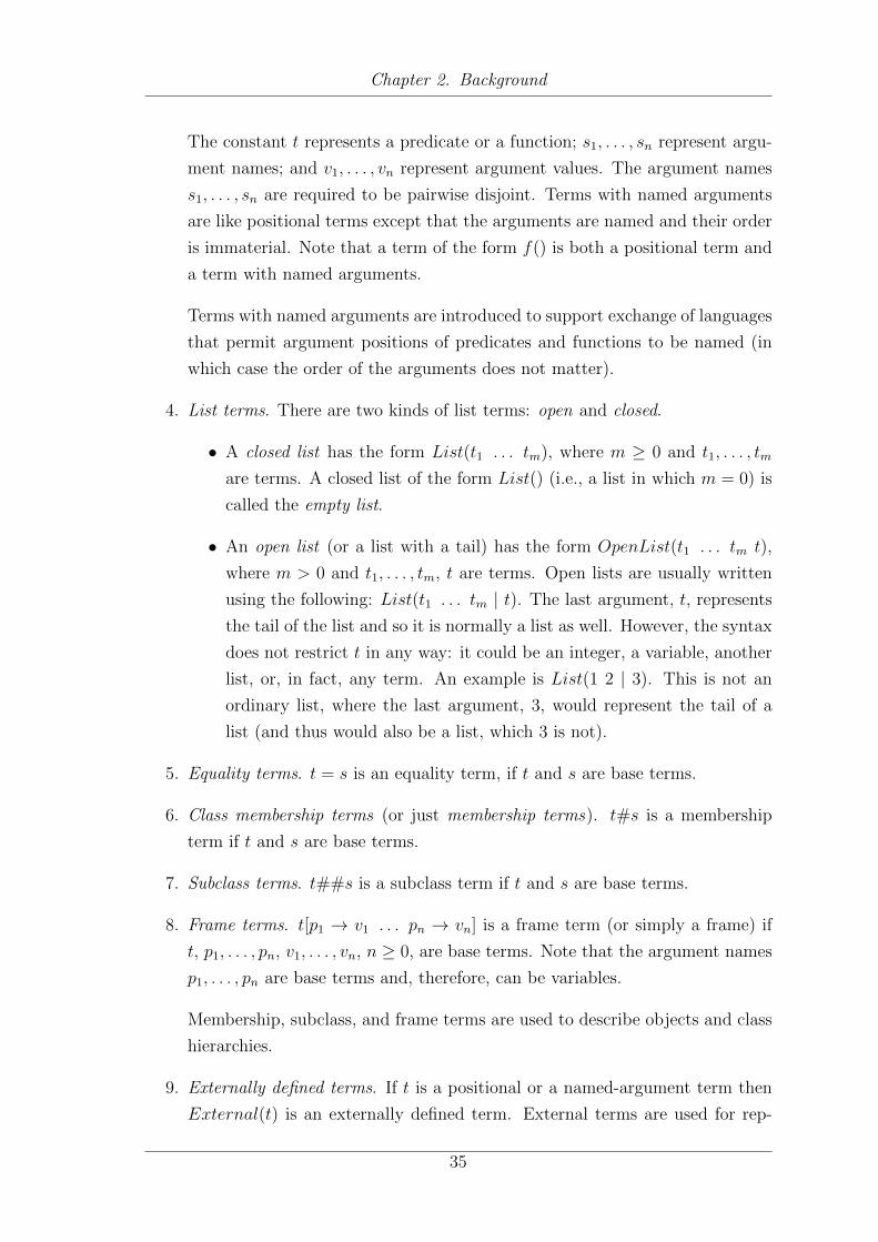
Chapter 2. Background
The constant t represents a predicate or a function; s1, . . . , sn represent argu-
ment names; and v1, . . . , vn represent argument values. The argument names
s1, . . . , sn are required to be pairwise disjoint. Terms with named arguments
are like positional terms except that the arguments are named and their order
is immaterial. Note that a term of the form f() is both a positional term and
a term with named arguments.
Terms with named arguments are introduced to support exchange of languages
that permit argument positions of predicates and functions to be named (in
which case the order of the arguments does not matter).
4. List terms. There are two kinds of list terms: open and closed.
• A closed list has the form List(t1 . . . tm), where m ≥ 0 and t1, . . . , tm
are terms. A closed list of the form List() (i.e., a list in which m = 0) is
called the empty list.
• An open list (or a list with a tail) has the form OpenList(t1 . . . tm t),
where m > 0 and t1, . . . , tm, t are terms. Open lists are usually written
using the following: List(t1 . . . tm | t). The last argument, t, represents
the tail of the list and so it is normally a list as well. However, the syntax
does not restrict t in any way: it could be an integer, a variable, another
list, or, in fact, any term. An example is List(1 2 | 3). This is not an
ordinary list, where the last argument, 3, would represent the tail of a
list (and thus would also be a list, which 3 is not).
5. Equality terms. t = s is an equality term, if t and s are base terms.
6. Class membership terms (or just membership terms). t#s is a membership
term if t and s are base terms.
7. Subclass terms. t##s is a subclass term if t and s are base terms.
8. Frame terms. t[p1 → v1 . . . pn → vn] is a frame term (or simply a frame) if
t, p1, . . . , pn, v1, . . . , vn, n ≥ 0, are base terms. Note that the argument names
p1, . . . , pn are base terms and, therefore, can be variables.
Membership, subclass, and frame terms are used to describe objects and class
hierarchies.
9. Externally defined terms. If t is a positional or a named-argument term then
External(t) is an externally defined term. External terms are used for rep-
35

Chapter 2. Background
resenting built-in functions and predicates as well as “procedurally attached”
terms or predicates, which might exist in various rule-based systems, but are
not specified by RIF.
Formulas
RIF-BLD allows the formalization of atomic formulas (Definition 2.3.3) and more
general formulas (e.g., disjunctions or conjunctions) constructed from atomic for-
mulas (Definition 2.3.4).
Definition 2.3.3. (Reproduced from [8, Section 2.3]) Any term (positional or with
named arguments) of the form p(. . .), where p is a predicate symbol, is an atomic
formula. Equality, membership, subclass, and frame terms are also atomic formulas.
An externally defined term of the form External(ϕ), where ϕ is an atomic formula,
is an atomic formula, called an externally defined atomic formula. Note that simple
terms (constants and variables) are not formulas.
Definition 2.3.4. (Reproduced from [8, Section 2.3]) A RIF-BLD formula can have
several different forms and is defined as follows:
1. Atomic: If ϕ is an atomic formula then it is also a formula.
2. Condition formula: A condition formula is either an atomic formula or a
formula that has one of the following forms:
• Conjunction: If ϕ1, . . . , ϕn, n ≥ 0, are condition formulas then so is
And(ϕ1 . . . ϕn), called a conjunctive formula. As a special case, And()
is allowed and is treated as a tautology, i.e., a formula that is always true.
• Disjunction: If ϕ1, . . . , ϕn, n ≥ 0, are condition formulas then so is
Or(ϕ1 . . . ϕn), called a disjunctive formula. As a special case, Or()
is permitted and is treated as a contradiction, i.e., a formula that is
always false.
• Existentials: If ϕ is a condition formula and ?V1, . . . , ?Vn, n > 0, are
distinct variables then Exists ?V1 . . .?Vn(ϕ) is an existential formula.
Condition formulas are intended to be used inside the premises of rules.
3. Rule implication: ϕ : − ψ is a formula, called rule implication, if:
• ϕ is an atomic formula or a conjunction of atomic formulas,
36

Chapter 2. Background
• ψ is a condition formula, and
• none of the atomic formulas in ϕ is an externally defined term (i.e., a
term of the form External(. . .)). Note: external terms can also occur in
the arguments of atomic formulas in the rule conclusion. For instance,
p(func:numeric-add(?X,"2"ˆˆxs:integer)) : − q(?X).
4. Universal rule: If ϕ is a rule implication and ?V1, . . . , ?Vn, n > 0, are distinct
variables then Forall ?V1...?Vn(ϕ) is a formula, called a universal rule. It is
required that all the free variables in ϕ occur among the variables ?V1 . . .?Vn
in the quantification part. An occurrence of a variable ?V is free in ϕ if it is
not inside a subformula of ϕ of the form Exists ?V (ψ) and ψ is a formula.
Universal rules will also be referred to as RIF-BLD rules.
5. Universal fact: If ϕ is an atomic formula and ?V1, . . . , ?Vn, n > 0, are dis-
tinct variables then Forall ?V1 . . .?Vn(ϕ) is a formula, called a universal fact,
provided that all the free variables in ϕ occur among the variables ?V1 . . .?Vn.
Universal facts are often considered to be rules without premises.
6. Group: If ϕ1, . . . , ϕn are RIF-BLD rules, universal facts, variable-free rule im-
plications, variable-free atomic formulas, or group formulas thenGroup(ϕ1 . . . ϕn)
is a group formula. As a special case, the empty group formula, Group(), is
allowed and is treated as a tautology, i.e., a formula that is always true.
Non-empty group formulas are used to represent sets of rules and facts. Note
that some of the ϕi’s can be group formulas themselves, which means that
groups can be nested.
7. Document: An expression of the form Document(directive1 . . . directiven Γ)
is a RIF-BLD document formula (or simply a document formula), if
• Γ is an optional group formula; it is called the group formula associated
with the document.
• directive1, . . . , directiven is an optional sequence of directives. A direc-
tive can be a base directive, a prefix directive or an import directive.
– A base directive has the form Base(< iri >), where iri is a Unicode
string in the form of an absolute IRI.
The Base directive defines a syntactic shortcut for expanding relative
IRIs into full IRIs, as described in [33, Section 2].
37

Chapter 2. Background
– A prefix directive has the form Prefix(p < v >), where p is an
alphanumeric string that serves as the prefix name and v is an ex-
pansion for p (a Unicode sequence of characters that forms an IRI).
An alphanumeric string is a sequence of ASCII characters, where
each character is a letter, a digit, or an underscore “ ”, and the first
character is a letter.
Like the Base directive, the Prefix directives define shorthands to
allow more concise representation of constants that come from the
symbol space rif:iri (we will call such constants rif:iri con-
stants) [33].
– An import directive can have one of two forms: Import(< loc >) or
Import(< loc > < p >). Here loc and p are Unicode sequences of
characters that form IRIs. The constants loc represents the location
of another document to be imported and is called the locator of
the imported document. The argument p is called the profile of
import. The profile p indicates what kind of entity is being imported
and under what semantics. If p is omitted it is required that the
imported document is again RIF-BLD document. Two-argument
import directives are provided to enable the import of other types of
documents, and their semantics are supposed to be covered by other
specifications, such as in [22].
A document formula can contain at most one Base directive. The Base
directive, if present, must be first, followed by any number of Prefix
directives, followed by any number of Import directives.
In the following, document formulas will be referred to as RIF-BLD doc-
uments.
In Definition 2.3.4, the component formulas ϕ, ϕi, ψi and Γ are said to be subfor-
mulas of the respective formulas (condition, rule, group, etc.) that are built using
these components.
RIF-BLD Annotations in the Presentation Syntax
Every term and formula, including terms and formulas that appear inside other
terms and formulas, can be annotated with an annotation of the form (∗ id ϕ ∗),
38

Chapter 2. Background
where id is a rif:iri constant and ϕ is a frame formula or a conjunction of frame
formulas. The id part is the identifier of the term or formula to be annotated and
the frame or the conjunction of frames is the metadata that should describe the
term or formula [8, Section 2.4].
Example 2.3.2. Listing 2.1 shows a RIF-BLD document, which defines a formula
expressing the statement that all persons who study computer science are considered
to be awesome. The group of the document formula is annotated with metadata
(line 6) using the Dublin Core vocabulary.13
Listing 2.1: RIF-BLD Annotations.
1 Document(
2 Prefix(ex <http://example.com/concepts#>)
3 Prefix(dc <http://purl.org/dc/terms/>)
4 Prefix(xs <http://www.w3.org/2001/XMLSchema#>)
5
6 (* _pd[dc:creator → "Adrian Marte"ˆˆxs:string *)
7 Group (
8 Forall ?Person (
9 ex:is-awesome(?Person) :- And(ex:person(?Person)
10 ex:studies(?Person ex:Computer-Science))
11 )
12 )
13 )
Well-formed Formulas
In order to avoid ambiguities when interpreting RIF-BLD documents and formulas,
RIF-BLD defines the notation of well-formed formulas. For a formula to qualify
as a well-formed formula, it is required that no constant appears in more than one
context, formally defined in Definition 2.3.5. For instance, in a well-formed formula
a constant that appears as an individual is not allowed to be a predicate name at
the same time.
The set of all constant symbols Const is partitioned into the following subsets:
• A subset of individuals. For instance, the symbols in Const that belong to the
symbol spaces of the datatypes defined in [8] are required to be individuals.
• A subset of plain (i.e., non-external) function symbols.
13Dublin Core, http://www.dublincore.org [last checked 10.03.2011]
39

Chapter 2. Background
• A subset of external function symbols.
• A subset of plain predicate symbols.
• A subset of external predicate symbols.
Definition 2.3.5. (Reproduced from [8, Section 2.4]) The context of an occurrence
of a symbol s ∈ Const in a formula ϕ is determined as follows:
• If s occurs as a predicate of the form s(...) (positional or named-argument) in
an atomic subformula of ϕ then s occurs in the context of a (plain) predicate
symbol.
• If s occurs as a predicate of the form s(...) (positional or named-argument) in
an atomic subformula of ϕ then s occurs in the context of a (plain) predicate
symbol.
• If s occurs as a function symbol in a non-subformula term of the form s(...)
then s occurs in the context of a (plain) function symbol.
• If s occurs as a predicate in an atomic subformula External(s(...)) then s
occurs in the context of an external predicate symbol.
• If s occurs as a function in a non-subformula term External(s(...)) then s
occurs in the context of an external function symbol.
• If s occurs in any other context (in a frame: s[...] or . . . [s→ ...] or ...[...→ s]
or in a positional or named-argument term p(... s ...) or q(... → s ...)), it is
said to occur as an individual.
As already mentioned, RIF-BLD documents allow the import of other documents,
which, in turn, can import further documents. The following definition formally
specifies the concept of imported documents. This definition is later required in
order to ensure that constants among imported documents do not appear in multiple
contexts.
Definition 2.3.6. (Reproduced from [8, Section 2.4]) Let ∆ be a document formula
and Import(loc) be one of its import directives, where loc is a locator of another
document formula ∆′. We say that ∆′ is directly imported into ∆.
A document formula ∆′ is said to be imported into ∆ if it is either directly imported
into ∆ or it is imported (directly or indirectly) into some other formula that is directly
imported into ∆.
40

Chapter 2. Background
The definition only deals with one-argument import directives, since only such di-
rectives can be used to import other RIF-BLD documents (Definition 2.3.4).
A well-formed formula is a RIF-BLD (document) formula where every constant sym-
bol appears in exactly one context, and all constant symbols other than rif:local
appearing in the directly or indirectly imported documents are required to occur in
exactly one context in the document and all imported documents. Moreover, every
externally defined term or formula must be an instantiation of a schema in a coher-
ent set of external schemas. The formal definition of well-formed formulas is shown
in Definition 2.3.7.
Definition 2.3.7. (Reproduced from [8, Section 2.4]) A formula ϕ is well-formed
iff:
• every constant symbol (whether coming from the symbol space rif:local
or not) mentioned in ϕ occurs in exactly one context.
• if ϕ is a document formula and ∆′1, ...,∆′k are all of its imported documents,
then every non-rif:local constant symbol mentioned in ϕ or any of the
imported ∆′i’s must occur in exactly one context (in all of the ∆′i’s).
• whenever a formula contains a term or a subformula of the form External(t),
t must be an instantiation of a schema in the coherent set of external schemas,
as specified in [8, Section 6], associated with the language of RIF-BLD.
• if t is an instantiation of a schema in the coherent set of external schemas
associated with the language then t can occur only as External(t), i.e., as an
external term or atomic formula.
Having defined the alphabet, terms and well-formed formulas we can now define the
language of RIF-BLD as in Definition 2.3.8.
Definition 2.3.8. (Reproduced from [8, Section 2.4]) The language of RIF-BLD
consists of the set of all well-formed formulas and is determined by the alphabet of
the language, as defined in Definition 2.3.1, and a set of coherent external schemas,
which determine the available built-ins and other externally defined predicates and
functions, as defined in [8, Section 6].
41

Chapter 2. Background
2.3.2.2. Semantics of RIF-BLD
RIF-BLD specifies model-theoretic semantics for RIF-BLD (document) formulas
[8, Section 3]. In model theory the semantics of a formal system are given by
their possible interpretations [10, page 148]. For RIF-BLD a semantic structure is
considered, consisting of a set of truth values, sets of universes and functions that
assign RIF-BLD terms to the corresponding values in the universes and formulas
to the corresponding truth values. Note that in the definitions only absolute IRIs
are used, i.e., all shortcuts (e.g., CURIE) have been expanded to the corresponding
absolute IRIs.
Definition 2.3.9. (Reproduced from [8, Section 3]) The set of truth values TV
consists of the values true and false.
Definition 2.3.10. (Reproduced from [8, Section 3]) A semantic structure I is a tu-
ple of the form < TV,DTS,D,Dind, Dfunc, IC , IV , IF , INF , Ilist, Itail, Iframe, Isub, Iisa,
I=, Iexternal, Itruth >. Here D is a non-empty set of elements called the domain of I,
and Dind, Dfunc are non-empty subsets of D. Dind is used to interpret the elements
of Const that occur as individuals and Dfunc is used to interpret the elements of
Const that occur in the context of function symbols. As before, Const denotes the
set of all constant symbols and V ar the set of all variable symbols. DTS denotes a
set of identifiers for datatypes. See [33] for the semantics of datatypes.
The other components of I are total mappings defined as follows:
1. IC maps Const to D. This mapping interprets constant symbols. In addition:
• If a constant c ∈ Const is an individual then it is required that IC(c) ∈Dind.
• If c ∈ Const is a function symbol (positional or with named arguments)
then it is required that IC(c) ∈ Dfunc.
2. IV maps V ar to Dind. This mapping interprets variable symbols.
3. IF maps D to total functions D∗ind → D (here D∗ind is a set of all finite sequences
over the domain Dind). This mapping interprets positional terms. In addition:
• If d ∈ Dfunc then IF (d) must be a function D∗ind → Dind.
• This means that when a function symbol is applied to arguments that
are individual objects then the result is also an individual object.
42

Chapter 2. Background
4. INF maps D to the set of total functions of the form
SetOfFiniteSets(ArgNames×Dind)→ D. This mapping interprets function
symbols with named arguments. In addition:
• If d ∈ Dfunc then INF (d) must be a function
SetOfFiniteSets(ArgNames×Dind) → Dind. This is analogous to the
interpretation of positional terms with two differences:
– Each pair < s, v > ∈ ArgNames×Dind represents an argument/-
value pair instead of just a value in the case of a positional term.
– The arguments of a term with named arguments constitute a finite
set of argument/value pairs rather than a finite ordered sequence of
simple elements. So, the order of the arguments does not matter.
5. Ilist and Itail are used to interpret lists. They are mappings of the following
form:
• Ilist : D∗ind → Dind
• Itail : D+ind ×Dind → Dind
In addition, these mappings are required to satisfy the following conditions:
• The function Ilist is injective (one-to-one).
• The set Ilist(D∗ind), henceforth denoted Dlist, is disjoint from the value
spaces of all data types in DTS.
• Itail(a1, . . . , ak, Ilist(ak+1, . . . , ak+m)) = Ilist(a1, . . . , ak, ak+1, . . . , ak+m).
Note that the last condition above restricts Itail only when its last argument
is in Dlist. If the last argument of Itail is not in Dlist, then the list is a general
open one and there are no restrictions on the value of Itail except that it must
be in Dind.
6. Iframe maps Dind to total functions of the form SetOfFiniteBags(Dind ×Dind)→ D.
This mapping interprets frame terms. An argument d ∈ Dind to Iframe rep-
resents an object and the finite bag {< a1, v1 >, ..., < ak, vk >} represents a
bag of attribute-value pairs for d. We will see shortly how Iframe is used to
determine the truth valuation of frame terms.
43

Chapter 2. Background
Bags (multi-sets) are used here because the order of the attribute/value pairs
in a frame is immaterial and pairs may repeat. Such repetitions arise naturally
when variables are instantiated with constants. For instance, o[?A→?B ?C →?D] becomes o[a→ b a→ b] if variables ?A and ?C are instantiated with the
symbol a while ?B and ?D are instantiated with b. (We shall see later that
o[a→ b a→ b] is equivalent to o[a→ b].)
7. Isub gives meaning to the subclass relationship. It is a mapping of the form
Dind ×Dind → D.
Isub will be further restricted below to ensure that the operator ## is transi-
tive, i.e., that c1##c2 and c2##c3 imply c1##c3.
8. Iisa gives meaning to class membership. It is a mapping of the form Dind ×Dind → D.
Iisa will be further restricted below to ensure that the relationships # and ##
have the usual property that all members of a subclass are also members of
the superclass, i.e., that o#cl and cl##scl imply o#scl.
9. I= is a mapping of the form Dind×Dind → D. It gives meaning to the equality
operator.
10. Itruth is a mapping of the form D → TV . It is used to define truth valuation
for formulas.
11. Iexternal is a mapping from the coherent set of schemas for externally de-
fined functions to total functions D∗ → D. For each external schema σ =
(?X1 ... ?Xn; τ) in the coherent set of external schemas associated with the
language, Iexternal(σ) is a function of the form Dn → D.
For every external schema σ associated with the language, Iexternal(σ) is as-
sumed to be specified externally in some document (hence the name external
schema). In particular, if σ is a schema of a RIF built-in predicate or function,
Iexternal(σ) is specified in [33] so that:
• If σ is a schema of a built-in function then Iexternal(σ) must be the function
defined in [33].
• If σ is a schema of a built-in predicate then Itruth ◦ (Iexternal(σ)) (the
composition of Itruth and Iexternal(σ), a truth-valued function) must be as
specified in [33].
44

Chapter 2. Background
The following mapping from terms to D is defined, which is denoted using the same
symbol I as the one used for semantic structures. This overloading is convenient
and creates no ambiguity.
• I(k) = IC(k), if k is a symbol in Const
• I(?V ) = IV (?V ), if ?V is a variable in V ar
• I(f(t1 ... tn)) = IF (I(f))(I(t1), ..., I(tn))
• I(f(s1 → v1 ... sn → vn)) = INF (I(f))({< s1, I(v1) >, ..., < sn, I(vn) >})
Here {...} is used to denote a set of argument/value pairs.
• For list terms, the mapping is defined as follows:
– I(List()) = Ilist(<>).
Here, <> denotes an empty list of elements of Dind. (Note that the
domain of Ilist is D∗ind, so D0ind is an empty list of elements of Dind.)
– I(List(t1 ... tn)) = Ilist(I(t1), ..., I(tn)), if n > 0.
– I(List(t1 ... tn | t)) = Itail(I(t1), ..., I(tn), I(t)), if n > 0.
• I(o[a1 → v1 ... ak → vk]) =
Iframe(I(o))({< I(a1), I(v1) >, ..., < I(an), I(vn) >})
Here {...} denotes a bag of attribute/value pairs. Jumping ahead, we note
that duplicate elements in such a bag do not affect the truth value of a frame
formula. Thus, for instance, [a→ b a→ b] and o[a→ b] always have the same
truth value.
• I(c1##c2) = Isub(I(c1), I(c2))
• I(o#c) = Iisa(I(o), I(c))
• I(x = y) = I=(I(x), I(y))
• I(External(t)) = Iexternal(σ)(I(s1), ..., I(sn)), if t is an instantiation of the
external schema σ = (?X1 ... ?Xn; τ) by substitution ?X1/s1 ... ?Xn/s1.
By definition, External(t) is well-formed only if t is an instantiation of an
external schema. Furthermore, by the definition of coherent sets of external
schemas, t can be an instantiation of at most one such schema, so I(External(t))
45

Chapter 2. Background
is well-defined.
Note that the definitions of INF and I(x = y) imply that the terms with named
arguments that differ only in the order of their arguments are mapped by I to the
same element in the domain. This implies that the equalities like t(a→ 1 b→ 2 c→3) = t(c→ 3 a→ 2 b→ 2) are tautologies in RIF-BLD.
The set DTS must include the datatypes described in [33, Section 2.3].
The datatype identifiers in DTS impose the following restrictions: given dt ∈ DTS,
let LSdt denote the lexical space of dt, V Sdt denote its value space, and Ldt : LSdt →V Sdt the lexical-to-value-space mapping, see [33, Section 2.3] for the definitions of
these concepts. Then the following must hold:
• V Sdt ⊆ Dind and
• For each constant "lit"ˆˆdt such that lit ∈ LSdt, IC("lit"ˆˆdt) =
Ldt(lit).
That is, IC must map the constants of a datatype dt in accordance with Ldt. RIF-
BLD does not impose restrictions on IC for constants in symbol spaces that are not
datatypes included in DTS.
RIF-BLD Annotations in the Semantics
Annotations, as described in Section 2.3.2.1, are not taken into account when in-
terpreting RIF-BLD terms and formulas. Consequently, they are removed before
the mappings are applied or the truth values are assigned to formulas using TV alI ,
which is defined below.
Interpretation of Non-document Formulas
In this section the interpretation of non-document document formulas with respect
to the semantic structure defined in Section 2.3.2.2 is discussed. In principle, TV alI
is used to determine the truth value of a non-document formula. Definition 2.3.11
shows the formal definition of TV alI .
Definition 2.3.11. (Reproduced from [8, Section 3.4]) Truth valuation for well-
formed formulas in RIF-BLD is determined using the following function, denoted
TV alI :
46

Chapter 2. Background
1. Positional atomic formulas: TV alI(r(t1 ... tn)) = Itruth(I(r(t1 ... tn)))
2. Atomic formulas with named arguments: TV alI(p(s1 → v1 ... sk → vk)) =
Itruth(I(p(s1 → v1 ... sk → vk))).
3. Equality: TV alI(x = y) = Itruth(I(x = y)).
To ensure that equality has precisely the expected properties, it is required that
Itruth(I(x = y)) = t if I(x) = I(y) and that Itruth(I(x = y)) = f otherwise.
This is equivalent to saying that TV alI(x = y) = t if and only if I(x) = I(y).
4. Subclass: TV alI(sc##cl) = Itruth(I(sc##cl)).
To ensure that the operator ## is transitive, i.e., c1##c2 and c2##c3 im-
ply c1##c3, it is required that for all c1, c2, c3 ∈ D if TV alI(c1##c2) =
TV alI(c2##c3) = t then TV alI(c1##c3) = t.
5. Membership: TV alI(o#cl) = Itruth(I(o#cl)).
To ensure that all members of a subclass are also members of the superclass,
i.e., o#cl and cl##scl imply o#scl, it is required that for all o, cl, scl ∈ D, if
TV alI(o#cl) = TV alI(cl##scl) = t then TV alI(o#scl) = t.
6. Frame: TV alI(o[a1 → v1 ... ak → vk]) = Itruth(I(o[a1 → v1 ... ak → vk])).
Since the bag of attribute/value pairs associated with an object o represents the
conjunction of assertions represented by these pairs, the following is required,
if k > 0, TV alI(o[a1 → v1 ... ak → vk]) = t if and only if TV alI(o[a1 → v1]) =
... = TV alI(o[ak → vk]) = t.
7. Externally defined atomic formula:
TV alI(External(t)) = Itruth(Iexternal(σ)(I(s1), ..., I(sn))), if t is an atomic for-
mula that is an instantiation of the external schema σ = (?X1 ... ?Xn; τ) by
substitution ?X1/s1 ... ?Xn/s1.
Note that, by definition, External(t) is well-formed only if t is an instantiation
of an external schema. Furthermore, by the definition of coherent sets of
external schemas, t can be an instantiation of at most one such schema, so
I(External(t)) is well-defined.
8. Conjunction: TV alI(And(c1 ... cn)) = t if and only if TV alI(c1) = ... =
TV alI(cn) = t. Otherwise, TV alI(And(c1 ... cn)) = f . As already mentioned,
the empty conjunction is treated as a tautology, so TV alI(And()) = t.
47

Chapter 2. Background
9. Disjunction: TV alI(Or(c1 ... cn)) = f if and only if TV alI(c1) = ... =
TV alI(cn) = f . Otherwise, TV alI(Or(c1 ... cn)) = t. As already mentioned,
the empty disjunction is treated as a contradiction, so TV alI(Or()) = f .
10. Quantification:
• TV alI(Exists ?v1 ... ?vn(ϕ)) = t if and only if for some I∗, described
below, TV alI∗(ϕ) = t.
• TV alI(Forall ?v1 ... ?vn(ϕ)) = t if and only if for every I∗, described
below, TV alI∗(ϕ) = t.
Here I∗ is a semantic structure of the form < TV,DTS,D,Dind, Dfunc, IC , I∗V ,
IF , INF , Ilist, Itail, Iframe, Isub, Iisa, I=, Iexternal, Itruth >, which is exactly like I,
except that the mapping I∗V , is used instead of IV . I∗V is defined to coincide
with IV on all variables except, possibly, on ?v1, ..., ?vn.
11. Rule implication:
• TV alI(conclusion : − condition) = t, if either TV alI(conclusion) = t
or TV alI(condition) = f .
• TV alI(conclusion : − condition) = f otherwise.
12. Groups of rules:
If Γ is a group formula of the form Group(ϕ1 ... ϕn) then
• TV alI(Γ) = t if and only if TV alI(ϕ1) = t, ..., TV alI(ϕn) = t.
• TV alI(Γ) = f otherwise.
This means that a group of rules is treated as a conjunction. In particular,
the empty group is treated as a tautology, so TV alI(Group()) = t.
Interpretation of Document Formulas
As RIF-BLD allows documents to import other documents, the notion of semantic
structure needs to be extended to semantic multi-structure in order to express multi-
document semantics, as shown in Definition 2.3.12. One interesting aspect of the
multi-document semantics is that rif:local symbols that belong to different
documents can have different meanings [8, Section 3.5].
48

Chapter 2. Background
Definition 2.3.12. (Reproduced from [8, Section 3.5]) A semantic multi-structure
I is a set of semantic structures of the form {J, I; I i1 , I i2 , ...}, where
• I and J are RIF-BLD semantic structures and
• I i1 , I i2 , etc., are semantic structures adorned with the locators of distinct RIF-
BLD formulas (one can think of these adorned structures as locator-structure
pairs).
All the structures in I (adorned and non-adorned) are identical in all respects except
for the following:
• The mappings JC , IC , ICi1 , ICi2 , ... may differ on the constants in Const that
belong to the rif:local symbol space.
As will be seen from the next definition, the structure I in the above is used to
interpret document formulas, and the adorned structures of the form I ik are used to
interpret imported documents. The structure J is used in the definition of entailment
for non-document formulas.
The semantics of RIF documents is now defined as follows.
Definition 2.3.13. (Reproduced from [8, Section 3.5]) Let ∆ be a document for-
mula and let ∆1, ...,∆n be all the RIF-BLD document formulas that are imported
(directly or indirectly) into ∆. Let Γ, Γ1, ...,Γn denote the respective group for-
mulas associated with these documents. Let I = {J, I; I i1 , ..., I in , ...} be a seman-
tic multi-structure that contains the semantic structures adorned with the locators
i1, ..., in of the documents ∆1, ...,∆n. Then we define: TV alI(∆) = t if and only if
TV alI(Γ) = TV alIi1 (Γ1) = ... = TV alIin (Γn) = t.
In order to apply TV alI to non-document formulas, the definition of TV alI has to
be extended as shown in Definition 2.3.14.
Definition 2.3.14. (Reproduced from [8, Section 3.5]) For non-document formulas,
we extend TV alI(ϕ) from regular semantic structures to multi-structures as follows.
Let I = {J, I; ...} be a semantic multi-structure. Then we define: TV alI(ϕ) =
TV alJ(ϕ).
49

Chapter 2. Background
Logical Entailment
Finally, the concept of logical entailment is defined for RIF-BLD rules using the
truth assignment defined in Definition 2.3.13 and 2.3.14. Logical entailment can be
used, for instance, to query RIF-BLD group or document formulas by checking if
a group or document formula entails a RIF-BLD condition formula (e.g., conjunc-
tion or disjunction). Logical entailment is formally defined in Definition 2.3.15 and
Definition 2.3.16.
Definition 2.3.15. (Reproduced from [8, Section 3.6]) A multi-structure I is a
model of a formula ϕ written as I |= ϕ, if and only if TV alI(ϕ) = t. Here, ϕ can be
a document or a non-document formula.
Definition 2.3.16. (Reproduced from [8, Section 3.6]) Let ϕ and ψ be (document
or non-document) formulas. We say that ϕ entails ψ, written as ϕ |= ψ, if and only
if for every multi-structure, I, I |= ϕ implies I |= ψ.
In the following, a system capable of entailment checking will be referred to as a
RIF-BLD reasoner or processor.
2.3.2.3. RIF-BLD Processor
RIF is a format for the interchange of rules. As such, it defines a presentation syntax
and a concrete XML syntax for representing rules and specifies the semantics thereof.
Furthermore, RIF specifies under which circumstances a system is considered a
conformant RIF processor (consumer and producer).
According to [8, Section 5], conformance is described in terms of semantics-preserving
transformations between the native syntax of a compliant system and the XML syn-
tax of RIF-BLD. Let T be a set of datatypes and symbol spaces that includes the
datatypes specified in [33], and the symbol spaces rif:iri, and rif:local. Sup-
pose E is a coherent set of external schemas that includes the built-ins listed in [33].
We say that a formula ϕ is a BLDT,E formula iff
• It is a well-formed BLD formula,
• All datatypes and symbol spaces used in ϕ are in T ,
• All externally defined terms used in ϕ are instantiations of external schemas
from E.
50

Chapter 2. Background
Definition 2.3.17. (Reproduced from [8, Section 5]) A RIF processor is a confor-
mant BLDT,E consumer iff it implements a semantics-preserving mapping, µ, from
the set of all BLDT,E formulas to the language L of the processor. Formally, this
means that for any pair ϕ, ψ of BLDT,E formulas for which ϕ |=BLD ψ is defined,
ϕ |=BLD ψ iff µ(ϕ) |=L µ(ψ). Here |=BLD denotes the logical entailment in RIF-BLD
and |=L is the logical entailment in the language L of the RIF processor.
Definition 2.3.18. (Reproduced from [8, Section 5]) A RIF processor is a confor-
mant BLDT,E producer iff it implements a semantics-preserving mapping, ν, from
the language L of the processor to the set of all BLDT,E formulas. Formally, this
means that for any pair ϕ, ψ of formulas in L for which ϕ |=L ψ is defined, ϕ |=L ψ
iff ν(ϕ) |=BLD ν(ψ).
Additionally, the following conformance clauses for RIF-BLD have been specified in
[8, Section 5].
• Conformant BLD producers and consumers are required to support only the
entailments of the form ϕ |=BLD ψ, where ψ is a closed RIF condition formula,
i.e., a RIF condition in which every variable, ?V , is in the scope of a quantifier
of the form Exists ?V . In addition, conformant BLD producers and consumers
should preserve all annotations where possible.
• A conformant BLD consumer must reject any document containing features it
does not support.
• A conformant BLD producer is a conformant BLDT,E producer, which pro-
duces documents that include only the datatypes and externals that are re-
quired by BLD.
51

3
RIF4J
This chapter describes RIF4J, a reasoning engine for RIF-BLD that provides a Java
object model for RIF-BLD and supports the parsing and serialization of RIF-BLD
formulas. Furthermore, it provides two prototype implementations of RIF-BLD
consumers based on the Datalog engines IRIS14 and IRIS-RDB (Chapter 4).
The RIF4J object model will be discussed in Section 3.2. Section 3.3 and Section
3.4 outline the XML parser and the XML and the presentation syntax serializer,
respectively. The two RIF-BLD consumers are presented in Section 3.5 and, finally,
the mapping from RIF-BLD to Datalog is defined in Section 3.6. An evaluation
of the two RIF-BLD consumers is provided in Section 5.1, which focuses on the
RIF-BLD conformance of the two systems.
3.1. Overview
RIF4J is a Java object model for the Basic Logic Dialect (BLD) of the Rule In-
terchange Format (RIF). It supports parsing of RIF-BLD documents in the XML
syntax and the serialization to the XML and presentation syntax of RIF-BLD. Fur-
thermore, it interfaces the concept of a RIF-BLD reasoner, which supports checking
for logical entailment of RIF-BLD condition formulas against a set of RIF-BLD
formulas, as shown in Section 2.3.2.2. The library also provides two prototype im-
plementations of a RIF-BLD reasoner based on the Datalog system IRIS and the
Datalog system IRIS-RDB developed in the course of this master thesis.
RIF4J is an open-source library licensed under the Apache License 2.0 and hosted on
14IRIS Reasoner, http://www.iris-reasoner.org [last checked 01.03.2011]
52
Chapter 3. RIF4J
Sourceforge15. The library has been applied in the integrated project LarKC, which
develops a platform for distributed and scalable reasoning. In particular, RIF4J is
being used in a parallelized Datalog system [16] currently under development, which
leverages techniques such as data and rule partitioning [17] and map-reduce-style
programming models [14]. It enables the system to parse and translate RIF-Core
formulas to equivalent Datalog expressions.
3.2. Object Model
The object model has been designed to reflect the presentation syntax as specified
by the EBNF grammar for RIF-BLD [8, Section 2.6], which provides a more concise
view of the syntax. Therefore, the naming of the classes may differ from the respec-
tive names in Section 2.3.2.1. Figure 3.1 shows a simplified class diagram of the
object model, where the focus lies on the class hierarchy rather than the relations
between the various classes.
On top of the class hierarchy resides the interface Describable, which denotes
RIF-BLD formulas and terms that can be annotated as described in Section 2.3.2.1.
A RIF-BLD document formula is represented by the class Document, for which a
Base and multiple Prefixes and Import directives can be defined. The Document
object encapsulates an optional Group object (representing a group formula), which,
in turn, contains other group formulas, universal facts, universal rules, rule implica-
tions, or atomic formulas. Both universal facts and universal rules are represented
by the ForallFormula class, which encapsulates a Clause object described be-
low. Rule is a marker interface representing a universal rule or a Clause, which
can be either a rule implication, represented by the class ImpliesFormula, or an
atomic formula. AtomicFormula is the marker interface for Atom (representing
a positional term with or without named arguments), EqualAtom (representing
an equality term), Frame (representing a frame term), MemberAtom (represent-
ing a class membership term) and SubclassAtom (representing a subclass term).
Although an externally defined term (positional or with named arguments), rep-
resented by the class ExternalFormula that encapsulates an Atom object, is -
strictly speaking - also an atomic formula, the EBNF grammar did not specifically
define it as such. In the class diagram, the ExternalFormula is on the same level
as the other RIF-BLD condition formulas AndFormula (representing a conjunc-
tion), OrFormula (representing a disjunction) and ExistsFormula (represent-
15RIF4J on Sourceforge, http://sourceforge.net/projects/rif4j/
53
Chapter 3. RIF4J
ing an existential). The marker interface Term abstracts RIF-BLD base terms and
lists, where the class List represents list terms, Variable denotes variable terms,
Constant denotes constant terms and Expression and ExternalExpression
represent functions and externally defined functions, respectively. Finally, the inter-
face Uniterm abstracts RIF-BLD positional terms.
Unlike other object models, RIF4J does not specify interfaces for all its objects,
which are then usually instantiated via dedicated factory objects. This approach is
usually considered, when multiple implementations of an object model are expected
to be developed. In the case of RIF4J, however, the object model is considered to be
the only implementation required and, therefore, the library provides concrete im-
plementations that can be directly instantiated using the constructor of the various
classes.
3.2.1. Mutability
All classes mentioned above can be considered mutable, in the sense that the ex-
ternally visible state can be changed after instantiation. This is realized through
setter methods that allow to modify the properties of an object. For instance, the
Document class has a method setGroup with which the group formula of the doc-
ument can be modified. This approach provides more flexibility and better usability,
since, unlike as for immutable objects, it is not required to create a new object each
time a possibly small change has to be applied to an object. On the other hand, the
user of the library has to take special care when modifying the objects to not end
up in an invalid system state.
3.2.2. Visitor Pattern
It is assumed that the object model for RIF-BLD will very unlikely change in the
future. Nevertheless, the library should provide means to easily implement new func-
tionality on top of the object model. For this, the visitor pattern has been applied on
the RIF4J object model, which allows for the implementation of new operations and
functionalities realized through a visitor without changing the classes or interfaces
on which the visitor operates. In the unlikely case that the object model needs to
be modified or new classes and interfaces are added, this is immediately reflected
in the system, as all relevant visitor interfaces and the respective implementations
need to be updated, since they break exactly in those places where the new features
54

Chapter 3. RIF4J
Fig
ure
3.1
.:R
IF4J
Ob
ject
Model
.
55

Chapter 3. RIF4J
need to be handled.
The idea of the visitor pattern is to use a structure of element classes, e.g. Term, each
of which has an accept(...) method taking a visitor object, e.g. TermVisitor,
for an argument.16 In Java, a visitor is an interface having a visit(...) method
for each element class it is supposed to handle, e.g., a TermVisitor may have the
methods visit(List list) or visit(Constant constant). The accept
method of an element class calls the visit(...) method for its class, e.g., a
Constant object would call the method TermVisitor#visit(Constant).
Various concrete visitor classes can then be implemented that perform a specific
operation or represent a specific functionality by implementing their respective
visit(...) methods.
RIF4J makes use of the visitor pattern and provides various implementations of
such, which implement the following functionality:
• Serialization of objects to the respective representation in both the RIF-BLD
presentation and the XML syntax.
• Normalization of RIF-BLD terms and formulas to a simplified representation
or a representation in disjunctive normal form.
• Transformation of RIF-BLD terms and formulas to equivalent Datalog ex-
pressions, as described in Section 3.6.
3.3. XML Parser
RIF4J supports the parsing of RIF-BLD formulas encoded in the RIF-BLD XML
syntax. The parser was implemented using the Java API for XML Processing
(JAXP) included in Java 1.6 and is based on the XML schema files specified in [8,
Section 9]. When parsing an RIF-BLD XML encoded formula, the XML document
is first validated against the XML Schema files and then loaded into a Document
Object Model (DOM), from which the relevant parts are extracted by successive ex-
ecutions of XPath queries. The information gathered by the XPath queries is used
to instantiate the respective objects of the RIF4J object model. To allow maximal
flexibility, the manual XML processing was favored over the automatic parsing of
XML files to an auto-generated object model using the Java Architecture for XML
16See http://en.wikipedia.org/w/index.php?title=Visitor_pattern&oldid=415606422 for more information [last checked 12.03.2011]
56

Chapter 3. RIF4J
Binding (JAXB).17
3.4. Serializers
As already mentioned in Section 3.2.2, RIF4J includes visitor implementations to
serialize RIF-BLD terms or formulas represented in the RIF4J object model to both
the presentation syntax and the XML syntax. Although, the presentation syntax
should not be used as concrete syntax for RIF-BLD, it is in some cases convenient
to use a compact representation of the formulas and terms, especially when it comes
to the debugging of an implementation.
3.5. Reasoning with Datalog
Based on the aforementioned object model and the specification of logical entail-
ment, an interface for a RIF-BLD reasoner is defined that is capable of checking
if a set of rules (embedded in a document or group) entails another RIF-BLD for-
mula. In principle, any concrete implementation of the interface manifests in the
translation from the RIF-BLD syntax to the syntax of the underlying RIF proces-
sor, as already mentioned in Section 2.3.2.3. Further, it is required that the target
systems supports the entailment relation. The translation is carried out using the
RIF4J object model and, usually, by implementing various visitors that handle the
transformation of the different RIF-BLD formulas and terms.
RIF4J provides two prototypical implementations of a RIF-BLD consumer, each of
which is based on the Datalog language:
RIF4J and IRIS: A RIF-BLD consumer based on the Datalog reasoner IRIS. It
supports various extensions such as negation as failure, function symbols and
equality in the rule head and provides support for all datatypes and built-ins
defined in [33]. IRIS relies on an in-memory evaluation implementation, and
hence, the amount of data that the system can process is limited by a single
computer’s memory. An overview of IRIS is given in Section 4.1.
RIF4J and IRIS-RDB A RIF-BLD consumer based on IRIS-RDB, an extension
of the Datalog reasoner IRIS that aims to overcome the limitations of the in-
17Java Architecture for XML Binding, http://java.sun.com/xml/downloads/jaxb.html[last checked 12.03.2011]
57

Chapter 3. RIF4J
memory implementation in IRIS by leveraging the close relationship of Datalog
and relational algebra. Unlike IRIS, IRIS-RDB lacks the support for list terms
and (non-externally) defined functions. IRIS-RDB is described in more detail
in Chapter 4.
Both systems are closely related to each other, as they share a common code base
including an object model for Datalog programs. Therefore, for both systems the
same implementation can be used, which translates any RIF-BLD formula to an
equivalent Datalog presentation encoded in the Datalog object model supported by
IRIS and IRIS-RDB. This translation is realized by taking advantage of the visitor
pattern described in Section 3.2.2 and the API for the manipulation of the IRIS
Datalog object model. In principle, various visitors have been implemented, where
each handles the transformation of a specific kind of formula, e.g., a TermTransla-
tor takes care of transforming RIF-BLD constants, variables or expressions to an
equivalent representation in Datalog.
The reasoning capabilities, i.e., checking for logical entailment of a RIF-BLD for-
mula, are realized by translating the premise document formula to a Datalog pro-
gram and the conclusion formula to a Datalog query and then check if the query
is entailed by the Datalog program. See Figure 3.2 for a depiction of the general
architecture of the reasoners.
Figure 3.2.: RIF-BLD reasoning architecture.
The translation of the RIF-BLD formulas is carried out in multiple steps: first the
formulas encoded in the RIF-BLD XML syntax are parsed into the object model
of RIF4J. Optionally, the formulas can be created programmatically using the con-
58

Chapter 3. RIF4J
structors provided by the classes of the RIF4J object model. As a second step, the
formulas are normalized and the body of the rules are converted to a representation
in disjunctive normal form. The formulas are then simplified such that there are
no disjunctions in a rule body and no conjunctions in the rule head. After this
step the rules have the form of Horn clauses and can be directly translated into
Datalog rules using the object model of IRIS. Section 3.6 gives a formal definition
of the translation, showing the syntactic and semantic correspondence of RIF-BLD
to Datalog language of IRIS and IRIS-RDB.
3.6. Mapping RIF-BLD to Datalog
In order to support RIF-BLD formulas, an implementation based on RIF4J and
IRIS is developed, that transforms RIF-BLD formulas to a semantically equivalent
Datalog program compatible with the IRIS reasoner. In the following, we formally
define the transformation steps that are required to transform a RIF-BLD formula
to a Datalog program. This transformation is inspired by the translation algorithm
to convert a WSML ontology to an equivalent Datalog program as defined in [19].
3.6.1. Transformations
The transformation of RIF-BLD formulas to Datalog rules is a composition of single
transformations steps, which are consecutively applied, starting from the original
RIF formulas. RIF-BLD annotations are removed before the transformations are
applied. In the following, we use R to denote the power set of RIF-BLD formulas.
Normalization of Condition Formulas. In a first step, the transformation τnf
is applied as a mapping R → R to normalize RIF-BLD condition formulas. This
normalization reduces the complexity of RIF-BLD formulas to bring them closer
to Datalog rules, i.e., Horn clauses. The most important aspect of this step is the
conversion of a formula to its representation in disjunctive normal form. Table 3.1
shows how the RIF-BLD formulas are normalized in detail, where the formulas are
written in the presentation syntax of RIF-BLD. The symbols F and G denote RIF-
BLD formulas and T , P and V denote base terms. The transformation rules are
applied in the given order until no rule can be applied anymore. Rule 1 applies
the normalization to each formula in a set of formulas. Rules 2 and 3 eliminate
occurrences of disjunctions and conjunctions with only one disjunct and conjunct,
59
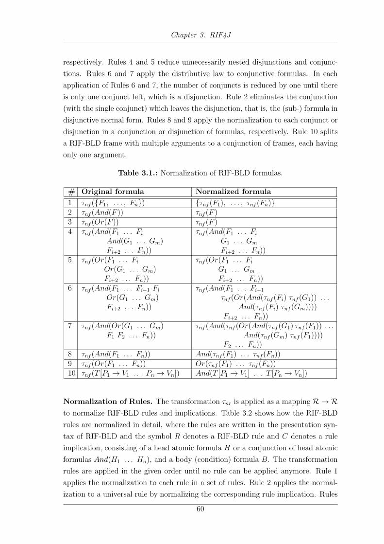
Chapter 3. RIF4J
respectively. Rules 4 and 5 reduce unnecessarily nested disjunctions and conjunc-
tions. Rules 6 and 7 apply the distributive law to conjunctive formulas. In each
application of Rules 6 and 7, the number of conjuncts is reduced by one until there
is only one conjunct left, which is a disjunction. Rule 2 eliminates the conjunction
(with the single conjunct) which leaves the disjunction, that is, the (sub-) formula in
disjunctive normal form. Rules 8 and 9 apply the normalization to each conjunct or
disjunction in a conjunction or disjunction of formulas, respectively. Rule 10 splits
a RIF-BLD frame with multiple arguments to a conjunction of frames, each having
only one argument.
Table 3.1.: Normalization of RIF-BLD formulas.
# Original formula Normalized formula
1 τnf ({F1, . . . , Fn}) {τnf (F1), . . . , τnf (Fn)}2 τnf (And(F )) τnf (F )3 τnf (Or(F )) τnf (F )4 τnf (And(F1 . . . Fi
And(G1 . . . Gm)Fi+2 . . . Fn))
τnf (And(F1 . . . Fi
G1 . . . Gm
Fi+2 . . . Fn))5 τnf (Or(F1 . . . Fi
Or(G1 . . . Gm)Fi+2 . . . Fn))
τnf (Or(F1 . . . Fi
G1 . . . Gm
Fi+2 . . . Fn))6 τnf (And(F1 . . . Fi−1 Fi
Or(G1 . . . Gm)Fi+2 . . . Fn))
τnf (And(F1 . . . Fi−1
τnf (Or(And(τnf (Fi) τnf (G1)) . . .And(τnf (Fi) τnf (Gm))))
Fi+2 . . . Fn))7 τnf (And(Or(G1 . . . Gm)
F1 F2 . . . Fn))τnf (And(τnf (Or(And(τnf (G1) τnf (F1)) . . .
And(τnf (Gm) τnf (F1))))F2 . . . Fn))
8 τnf (And(F1 . . . Fn)) And(τnf (F1) . . . τnf (Fn))9 τnf (Or(F1 . . . Fn)) Or(τnf (F1) . . . τnf (Fn))10 τnf (T [P1 → V1 . . . Pn → Vn]) And(T [P1 → V1] . . . T [Pn → Vn])
Normalization of Rules. The transformation τnr is applied as a mapping R → Rto normalize RIF-BLD rules and implications. Table 3.2 shows how the RIF-BLD
rules are normalized in detail, where the rules are written in the presentation syn-
tax of RIF-BLD and the symbol R denotes a RIF-BLD rule and C denotes a rule
implication, consisting of a head atomic formula H or a conjunction of head atomic
formulas And(H1 . . . Hn), and a body (condition) formula B. The transformation
rules are applied in the given order until no rule can be applied anymore. Rule 1
applies the normalization to each rule in a set of rules. Rule 2 applies the normal-
ization to a universal rule by normalizing the corresponding rule implication. Rules
60
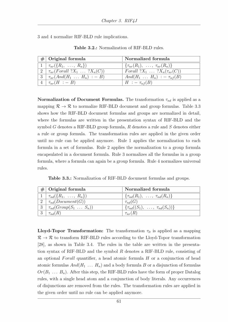
Chapter 3. RIF4J
3 and 4 normalize RIF-BLD rule implications.
Table 3.2.: Normalization of RIF-BLD rules.
# Original formula Normalized formula
1 τnr({R1, . . . , Rn}) {τnr(R1), . . . , τnr(Rn)}2 τnr(Forall ?X1 . . . ?Xn(C)) Forall ?X1 . . . ?Xn(τnr(C))3 τnr(And(H1 . . . Hn) : − B) And(H1 . . . Hn) : − τnf (B)4 τnr(H : − B) H : − τnf (B)
Normalization of Document Formulas. The transformation τnd is applied as a
mapping R → R to normalize RIF-BLD document and group formulas. Table 3.3
shows how the RIF-BLD document formulas and groups are normalized in detail,
where the formulas are written in the presentation syntax of RIF-BLD and the
symbol G denotes a RIF-BLD group formula, R denotes a rule and S denotes either
a rule or group formula. The transformation rules are applied in the given order
until no rule can be applied anymore. Rule 1 applies the normalization to each
formula in a set of formulas. Rule 2 applies the normalization to a group formula
encapsulated in a document formula. Rule 3 normalizes all the formulas in a group
formula, where a formula can again be a group formula. Rule 4 normalizes universal
rules.
Table 3.3.: Normalization of RIF-BLD document formulas and groups.
# Original formula Normalized formula
1 τnd({R1, . . . , Rn}) {τnd(R1), . . . , τnd(Rn)}2 τnd(Document(G)) τnd(G)3 τnd(Group(S1 . . . Sn)) {τnd((S1), . . . , τnd(Sn))}3 τnd(R) τnr(R)
Lloyd-Topor Transformation: The transformation τlt is applied as a mapping
R → R to transform RIF-BLD rules according to the Lloyd-Topor transformation
[28], as shown in Table 3.4. The rules in the table are written in the presenta-
tion syntax of RIF-BLD and the symbol R denotes a RIF-BLD rule, consisting of
an optional Forall quantifier, a head atomic formula H or a conjunction of head
atomic formulas And(H1 . . . Hn) and a body formula B or a disjunction of formulas
Or(B1 . . . Bn). After this step, the RIF-BLD rules have the form of proper Datalog
rules, with a single head atom and a conjunction of body literals. Any occurrences
of disjunctions are removed from the rules. The transformation rules are applied in
the given order until no rule can be applied anymore.
61

Chapter 3. RIF4J
Rule 1 applies the transformation to each rule in a set of rules. Rules 2 and 4
transform rules with a conjunction of atomic formulas in the head to multiple rules
with only a single head atomic formula. Similarly, Rules 3 and 5 create multiple
rules for rules with a disjunction of formulas in the body.
Table 3.4.: Lloyd-Topor transformation of RIF-BLD rules.
# Original rule Transformed rule
1 τlt({R1, . . . , Rn}) {τlt(R1), . . . , τlt(Rn)}2 τlt((Forall ?X1 . . .?Xm
(And(H1 . . . Hn) : − B))){τlt((Forall ?X1 . . .?Xm
(H1 : − B))), . . .τlt((Forall ?X1 . . .?Xm
(Hn : − B)))}3 τlt((Forall ?X1 . . .?Xm
(H : − Or(B1 . . . Bn)))){τlt((Forall ?X1 . . .?Xm
(H : − B1))), . . .τlt((Forall ?X1 . . .?Xm
(H : − Bn)))}4 τlt(And(H1 . . . Hn) : − B) {τlt(H1 : − B), . . . , τlt(Hn : − B)}5 τlt(H : − Or(B1 . . . Bn)) {τlt(H : − B1), . . . , τlt(H : − Bn)}
Datalog Rule Generation: In a final step, the transformation τdlog is applied as
a mapping R → P , where R is the power set of RIF-BLD formulas and terms and
P is the power set of Datalog rules, literals and terms. The transformation rules
are shown in Table 3.5, Table 3.6, Table 3.7 and Table 3.8. The RIF-BLD formulas
in the tables are written in the presentation syntax of RIF-BLD and the Datalog
rules and terms are written in the IRIS Datalog syntax. The symbol A represents
a RIF-BLD formula, rule or term, where a rule consists of a head atomic formula
H and a body condition formula B. F represents a RIF-BLD condition formula, X
denotes a variable, S, T , U , P and V denote terms, C, D and E are constants and
N is a string representing of a name. The transformation rules are applied in the
given order until no rule can be applied anymore.
Rule 1 in Table 3.5 applies the generation to each element in the set of RIF-BLD
formulas. Rules 2 to 4 generate the Datalog equivalent for a (universally quantified)
rule, where Rule 3 also takes into account an external expression appearing in the
head atomic formula.
Rule 5 in Table 3.6 creates a conjunction of Datalog literals for a conjunction of
RIF-BLD condition formulas. Rule 6 removes the existential quantifier from a RIF-
BLD formula, which is valid according to [28], since existential quantified formulas
can only occur in the body of a rule. Rules 7, 8 and 9 create a literal for a RIF-
62

Chapter 3. RIF4J
Table 3.5.: Datalog rule generation for RIF-BLD rules.
# Original formula, rule or term Datalog rule or term
1 τdlog(A1, . . . , An}) {τdlog(A1), . . . , τdlog(An)}2 τdlog((Forall ?X1 . . .?Xm (H : − B))) τdlog(H : − B).3 τdlog(C(T1, . . . , Ti,
External(D(S1 . . . Sm)),Ti+2, . . . , Tn) : − B)
τdlog(C(T1, . . . , Ti,?R, Ti+2, . . . , Tn) : −
τnf (And(B External(D(S1 . . . Sm, ?R)))))
4 τdlog(H : − B) τdlog(H) : − τdlog(B).
BLD atomic formula or a functional symbol in the case of a RIF-BLD expression.
Since IRIS does not support named arguments, Rule 8 orders the named argu-
ments according to the argument names in ascending order and omits the names in
the corresponding Datalog literals. Rule 7 handles atomic formulas with external
expressions as an argument. According to [8], external expressions represent built-
in functions defined in an external schema, such as RIF-DTB, which are directly
mapped to Datalog built-in functions. In IRIS, built-in functions do not “return”
a value, but store the result in the term at the last position. Consequently, Rule 7
creates a unique variable ?R for the result of the function and appends this variable
to the list of terms of the literal representing the built-in. This literal is then added
to the set of literals and ?R replaces the occurrence of the built-in in the original
atom. The generation is analogously applied to externally defined predicates and
functions in Rules 10 to 12.
Rules 13 to 24 in Table 3.7 generate the Datalog expressions for the equality, sub-
class, member and frame atomic formulas, respectively, also taking into account
arguments that are RIF-BLD external expression. The subclass, member and frame
atomic formulas are replaced by special meta-level predicates pmo, psco and phval that
represent their respective RIF-BLD constructs. The semantics for the correspond-
ing RIF-BLD language constructs are encoded in the meta-level axioms defined in
Table 3.9. Rules 25 and 26 generate Datalog lists for RIF-BLD lists, where one
of the arguments may also be an external expression. Rule 27 creates a Datalog
variable for a RIF-BLD variable using the same variable symbol.
Rules 28 to 34 in Table 3.8 generate Datalog literals for RIF-BLD frames, also taking
into account RIF-BLD external expression arguments. Similarly as in Rules 17 to
24, a special meta-level predicate phval is used.
The resulting Datalog rules are of the form H : − B1, . . . , Bn, where H is a
63

Chapter 3. RIF4J
Table 3.6.: Datalog rule generation for RIF-BLD condition formulas.
# Original formula, rule or term Datalog rule or term
5 τdlog(And(F1 . . . Fn)) τdlog(F1), . . . , τdlog(Fn)6 τdlog(Exists ?X1 . . .?Xm (F )) τdlog(F )7 τdlog(C(T1 . . . Ti
External(D(S1 . . . Sm)) . . .Ti+2 . . . Tn))
τdlog(C(T1, . . . , Ti?R, Ti+2, . . . , Tn)),
τdlog(D(S1, . . . , Sm, ?R))8 τdlog(C(N1 → V1 . . . Nn → Vn)) τdlog(C(V1, . . . , Vn))9 τdlog(C(T1 . . . Tn)) τdlog(C)(τdlog(T1), . . . , τdlog(Tn))10 τdlog(External(C(T1 . . . Ti
External(D(S1 . . . Sm)) . . .Ti+2 . . . Tn)))
τdlog(External(C(T1, . . . , Ti?R, Ti+2, . . . , Tn))),
τdlog(D(S1, . . . , Sm, ?R))11 τdlog(External(C(N1 → V1 . . .
Nn → Vn)))τdlog(C)(τdlog(V1), . . . , τdlog(Vn))
12 τdlog(External(C(T1 . . . Tn))) τdlog(C)(τdlog(T1), . . . , τdlog(Tn))
single literal in the head and the Bi’s are a conjunction of literals in the body of the
rule. In the tables formal definition of τdlog(C) is omitted, i.e. the transformation of
RIF-BLD constants to Datalog constant terms. In principal, a RIF-BLD constant
of a certain type is mapped to an equivalent Datalog constant term of the same
type. This is possible for IRIS, since IRIS supports all datatypes defined in [33],
which are required for any RIF-BLD conformant system.
Final Transformation: Finally, we define the transformation τ for converting
RIF-BLD formulas into the corresponding Datalog constructs as a composition τ =
τdlog ◦ τtp ◦ τnd ◦ τnr ◦ τnf . This mapping τ : R → P applies the single steps to
a RIF-BLD (document) formula, rule or term R ∈ R and yields a semantically
equivalent Datalog program τ(R) = P ∈ P when interpreted using the meta-level
axioms discussed below.
3.6.2. RIF-BLD Semantics Through Meta-Level Axioms
A fixed set of Pmeta ∈ P of Datalog rules, shown in Table 3.9, forms the meta-level
axioms which assure that the original RIF-BLD semantics are properly maintained.
There, C1, C2 and C3 denote terms that represent class identifiers and I denotes
a term that represents an instance identifier. Axiom 1 realizes transitivity for the
RIF-BLD Member construct and Axiom 2 ensures that an instance of a subclass is
also an instance of its superclass.
64

Chapter 3. RIF4J
Table 3.7.: Datalog rule generation for RIF-BLD atomic formulas.
# Original formula, rule or term Datalog rule or term
13 τdlog(External(C(S1 . . . Sl)) =External(D(U1 . . . Um)))
?R1 = ?R2,τdlog(C(S1, . . . , Sl, ?R1)),τdlog(D(U1, . . . , Um, ?R2))
14 τdlog(External(C(S1 . . . Sm)) = T1) ?R = τdlog(T1),τdlog(C(S1, . . . , Sm, ?R))
15 τdlog(T1 = External(C(S1 . . . Sm))) τdlog(T1) = ?R,τdlog(C(S1, . . . , Sm, ?R))
16 τdlog(T1 = T2) τdlog(T1) = τdlog(T2)17 τdlog(External(C(S1 . . . Sl)) #
External(D(U1 . . . Um)))pmo(?R1, ?R2),τdlog(C(S1, . . . , Sl, ?R1)),τdlog(D(U1, . . . , Um, ?R2))
18 τdlog(External(C(S1 . . . Sm)) # T1) pmo(?R, τdlog(T1)),τdlog(C(S1, . . . , Sm, ?R))
19 τdlog(T1 # External(C(S1 . . . Sm))) pmo(τdlog(T1), ?R),τdlog(C(S1, . . . , Sm, ?R))
20 τdlog(T1 # T2) pmo(τdlog(T1), τdlog(T2))21 τdlog(External(C(S1 . . . Sl)) ##
External(D(U1 . . . Um)))psco(?R1, ?R2),τdlog(C(S1, . . . , Sl, ?R1)),τdlog(D(U1, . . . , Um, ?R2))
22 τdlog(External(C(S1 . . . Sm)) ## T1) psco(?R, τdlog(T1)),τdlog(C(S1, . . . , Sm, ?R))
23 τdlog(T1 ## External(C(S1 . . . Sm))) psco(τdlog(T1), ?R),τdlog(C(S1, . . . , Sm, ?R))
24 τdlog(T1 ## T2) psco(τdlog(T1), τdlog(T2))25 τdlog(List(T1 . . . , Ti,
External(C(S1 . . . Sm)),Ti+2, . . . , Tn))
τdlog(List(T1, . . . , Ti,?R, Ti+2, . . . , Tn)),
τdlog(C(S1, . . . , Sm, ?R))26 τdlog(List(T1 . . . Tn)) [τdlog(T1), . . . , τdlog(Tn)]27 τdlog(?X) ?X
3.6.3. Logical Entailment Checking with Datalog Queries
RIF-BLD logical entailment [8] checking of a formula ψ against a set of rules, em-
bedded in a group or a document formula ϕ, is realized by posing Datalog queries
corresponding to ψ to a Datalog program corresponding to ϕ. For this, a Datalog
program Pϕ = Pmeta ∪ τ(ϕ) is generated that consists of the meta-level axioms to-
gether with the Datalog rules and facts corresponding to the group or document
formula. Each query Qi(−→xi ) in the set of queries R = τ(ψ) is evaluated against Pϕ,
written as (Pϕ, ?−Qi(−→xi )), which yields the set of all tuples
−→ti that instantiate the
65

Chapter 3. RIF4J
Table 3.8.: Datalog rule generation for RIF-BLD frames.
# Original formula, rule or term Datalog rule or term
28 τdlog(External(C(T1 . . . Tl))[External(D(S1 . . . Sm))→External(E(U1 . . . Un))])
phval(?R1, ?R2, ?R3),τdlog(C(T1, . . . , Tl, ?R1)),τdlog(D(S1, . . . , Sm, ?R2)),τdlog(E(U1, . . . , Un, ?R3))
29 τdlog(External(C(T1 . . . Tl))[External(D(S1 . . . Sm))→ U ])
phval(?R1, ?R2, τdlog(U)),τdlog(C(T1, . . . , Tl, ?R1)),τdlog(D(S1, . . . , Sm, ?R2))
30 τdlog(External(C(T1 . . . Tl))[S → External(D(U1 . . . Um))])
phval(?R1, τdlog(S), R2),τdlog(C(T1, . . . , Tl, ?R1)),τdlog(D(U1, . . . , Um, ?R2))
31 τdlog(T [External(C(S1 . . . Sl))→External(D(U1 . . . Um))])
phval(τdlog(T ), ?R1, ?R2),τdlog(C(S1, . . . , Sl, ?R1)),τdlog(D(U1, . . . , Um, ?R2))
32 τdlog(T [S → External(C(U1 . . . Ul))]) phval(τdlog(T ), τdlog(S), ?R1),τdlog(C(U1, . . . , Ul, ?R1))
33 τdlog(T [External(C(S1 . . . Sl))→ U ]) phval(τdlog(T ), ?R1, τdlog(U)),τdlog(C(S1, . . . , Sl, ?R1))
34 τdlog(T [P → V ]) phval(τdlog(T ), τdlog(P ), τdlog(V ))
Table 3.9.: RIF-BLD semantics in Datalog.
# Meta-Level Axiom
1 psco(C1, C3) : − psco(C1, C2), psco(C2, C3).2 pmo(I1, C2) : − pmo(I1, C1), psco(C1, C2).
vector −→xi of variables in the query such that Qi(−→ti ) is satisfied in the model of Pϕ.
If Qi(−→ti ) contains no variables, the query either evaluates to {Qi} if Qi is satisfied
in the model of Pϕ or ∅ otherwise. We say that ϕ entails ψ or ϕ � ψ if and only if
for all Qi(−→xi ) in R it is the case that (Pϕ, ?−Qi(
−→xi )) 6= ∅.
66

4
IRIS-RDB
This chapter describes IRIS-RDB, an extension of the Datalog reasoner IRIS that
uses a relational database as an underlying system to evaluate stratified and recursive
Datalog programs by taking advantage of relational algebra. IRIS-RDB has been
developed with the goal to have a more scalable reasoning engine that is able to
process knowledge bases that exceed the limits of a single computer’s memory. The
system has been developed in the context of the integrated project SOA4All and
has been reported in [30].
Section 4.2 outlines the problem of the original IRIS implementation. Section 4.3
describes the features of the software in detail. The Datalog evaluation process is
described in Section 4.4 and the description of the transformation from Datalog
programs to relational algebra is given in Section 4.5. Appendix B.2 shows how to
install and use the system for evaluating Datalog programs. An evaluation of the
software component is provided in Section 5.2 that focuses on the comparison of
IRIS and IRIS-RDB.
4.1. IRIS
The Integrated Rule Inference System (IRIS) is an open-source, Java-based Datalog
reasoning engine. It supports (un-) safe Datalog with (locally) stratified or well-
founded “negation as failure”, function symbols, equality in the rule head and a
comprehensive and extensible set of built-ins and datatypes [21] adopted from RIF-
DTB [33]. IRIS can be used as core engine for different reasoners that tackle diverse
formalism ranging across various OWL 2 [20] and WSML [13] dialects. It is the main
67

Chapter 4. IRIS-RDB
underlying engine used by the WSML2Reasoner framework [25] for reasoning with
WSML-Core, WSML-Flight and WSML-Rule variants.18 Recently [41][40], devel-
opment started on making the IRIS engine a conformant – or at least a maximally
compatible – RIF-BLD [8] processor.
IRIS is released under the GNU Lesser General Public License (LGPL) and provided
as a Java implementation that can be downloaded in both, source and binary form,
from the Sourceforge project page19. The extension described in this chapter, called
IRIS-RDB, is an additional module of IRIS and is, therefore, also licensed under
LGPL and is available on the same Sourceforge page.
4.2. Problems with IRIS
In IRIS the evaluation of Datalog queries, i.e., the evaluation of queries over a
knowledge base, where the knowledge base consists of facts and rules, is only handled
in memory. As RIF especially targets application to the Web, where the amount
of data is extremely large, IRIS-RDB has been developed with the goal to have a
more scalable reasoning engine that is able to process knowledge bases consisting
of facts that exceed the limits of a single computer’s memory. This is accomplished
by leveraging the close relationship of Datalog and relational algebra and, thus, by
implementing an evaluation strategy based on a relational database system.
4.3. Features of IRIS and IRIS-RDB
IRIS-RDB is an extension of the IRIS reasoner that uses the database engine H2
(version 1.3.148) as an underlying relational database system to evaluate Datalog
programs.20 H2 is an open-source relational database implemented in Java. It is a
very fast and feature-rich system that supports persistent and in-memory storage
and has both an embedded and a server mode. H2 is dual licensed under a modified
version of the MPL 1.1 (Mozilla Public License) and under the (unmodified) EPL
1.0 (Eclipse Public License). Since IRIS-RDB uses SQL as query language it is, in
principle, easy to align the system such that it is possible to use it with a different
18WSML2Reasoner framework, http://tools.sti-innsbruck.at/wsml2reasoner/ [lastchecked 15.03.2011]
19IRIS on Sourceforge, http://sourceforge.net/projects/iris-reasoner/ [lastchecked 24.01.2011]
20H2 Database Engine, http://www.h2database.com [last checked 19.01.2011]]
68

Chapter 4. IRIS-RDB
relational database engine than H2.
IRIS-RDB can evaluate safe or unsafe Datalog (without function symbols) and equal-
ity in rule heads, supports all datatypes and built-ins defined in RIF-DTB [33] and
provides support for (locally) stratified negation as failure (cf. Section 2.2.5). IRIS-
RDB makes heavy use of the interfaces and classes defined by IRIS and provides
implementations and extensions thereof where possible, which allows for the seam-
less integration of the extension into the IRIS code base. Table 4.1 gives an overview
of the different features supported in IRIS and IRIS-RDB.
Table 4.1.: Comparison of IRIS and IRIS-RDB features.
Feature IRIS IRIS-RDB
Unsafe rules Yes YesLocally stratified rules Yes YesEquality in rule heads Yes YesFunction symbols Yes NoList terms Yes NoRIF-DTB datatypes Yes YesRIF-DTB built-ins Yes YesRule head equality Yes Yes
As can be seen from the table, IRIS-RDB does not support function symbols and list
terms. The version of the semi-naive algorithm implemented in IRIS-RDB does not
deal with function symbols, therefore, function symbols are not allowed to appear
in Datalog programs handled by IRIS-RDB. The support of list terms is not given,
as the method for evaluating equality in rule heads implemented in IRIS-RDB does
not support list terms. The following sections describe the features of both IRIS
and IRIS-RDB in more detail.
4.3.1. Supported Datatypes
IRIS, and also IRIS-RDB, support all datatypes defined in RIF-DTB [33], in par-
ticular all XML Schema 1.1, RDF (rdf:XMLLiteral and rdf:PlainLiteral
[3]) and the RIF internal (rif:iri and rif:local) datatypes.
69

Chapter 4. IRIS-RDB
4.3.2. Built-in Predicates
IRIS supports a rich set of built-in predicates, which can be used in the bodies of
rules, both in positive and in negative literals. They include:
• Equality, inequality, assignment, and unification.
• Addition, subtraction, multiplication, division and modulus.
• All built-ins defined in RIF-DTB, including arithmetical built-ins, guard pred-
icates for datatypes, built-ins for datatype conversion and casting and special
functions and predicates on various RDF and XML Schema datatypes.
IRIS-RDB uses the built-in infrastructure of the original IRIS and, therefore, takes
advantage of all the built-ins mentioned above.
4.3.3. Rule Head Equality
In order to support rules with equality in the head, IRIS-RDB uses the rewriting
technique defined in [39, Section 4.1] where additional rules are created for each
predicate occurring in the Datalog program in order to resolve equivalent terms.
4.4. Rule Evaluation Process
IRIS-RDB evaluates queries over sets of facts (ground atomic formulas) and rules,
which together are called a knowledge base. A knowledge base can be created directly
via the Java API or can be parsed from a Datalog program in textual form using
the parser provided by IRIS. For each query that is evaluated over the knowledge
base, IRIS-RDB returns the set of tuples that can be found or inferred from the
knowledge base that satisfy the query.
IRIS-RDB supports semi-naive bottom-up evaluation (Algorithm A.3 in Appendix A)
using a (locally) stratified technique. The implementation of this evaluation strat-
egy is based on the original semi-naive implementation of IRIS and makes heavy
use of the involved interfaces and classes. See Figure 4.1 for a depiction of the steps
involved in the process of evaluation.
70

Chapter 4. IRIS-RDB
Figure 4.1.: Stratified evaluation strategy.
4.4.1. Program Optimization
The Magic Sets optimization technique [2] re-writes the rule-set according to the
query so that only tuples likely to be involved in satisfying the query are computed.
The disadvantage of this approach is that a new sub-set of the model must be
computed for each new query. Therefore, Magic Sets allows faster knowledge-base
initialization times at the expense of longer query times. IRIS can be configured
programmatically whether to use the Magic Sets optimization or not.
Another simpler program optimization technique is rule-filtering that simply re-
moves those rules that cannot influence the query result, therefore, reducing the
size of the minimal model computation. This technique is usually used in combina-
tion with Magic Sets.
71

Chapter 4. IRIS-RDB
4.4.2. Rule Safety Processing
The algorithm for detecting unsafe rules was used from the original IRIS implemen-
tation, which is based on the algorithm and the definition of unsafe rules defined
in [35, page 105]. According to this definition, a rule is safe if all its variables are
limited, where limited variables are defined as follows:21
1. Any variable that appears as an argument in an ordinary predicate of the body
is limited.
2. Any variable X that appears in a subgoal X = a or a = X, where a is a
constant, is limited.
3. Variable X is limited if it appears in a subgoal X = Y or Y = X, where Y is
a variable already known to be limited.
In order to support unsafe rules, IRIS provides an augmenting rule processor, which
is based on the technique suggested by [38] that adds a “universe” predicate for each
unbound variable to the body of the rule. This “universe” predicate contains all
constants appearing in the input program or that are created during the evaluation
of the program. For instance, consider rule
q(?X) : − not p(?X).
which unsafeness is directly visible, as variable X is not limited, since it does not
appear in any non-negated ordinary predicate, nor is it equated with a constant or a
variable known to be limited. However, using the aforementioned technique the rule
can be made safe by adding a universe predicate and, thus, limiting the variable X,
such that the new rule looks like
q(?X) : − universe(?X), not p(?X).
4.4.3. Stratification
IRIS has the concepts of globally and locally stratified logic programs. A glob-
ally stratified program is one where all rules can be grouped into strata using, for
21See also Section 2.2.4.1.
72

Chapter 4. IRIS-RDB
instance, the algorithm defined in [35, page 133]. This algorithm computes a strat-
ification of the rules of a program. It groups the predicates into strata, which are
the largest sets of predicates, such that:
1. If a predicate p is the head of a rule with a subgoal that is a negated q, then
q is in a lower stratum than p.
2. If predicate p is the head of a rule with a subgoal that is a non-negated q, then
the stratum of p is at least as high as the stratum of q.
Given stratified predicates the rules can also be grouped into strata, by assigning
rule r to stratum i, where i is the stratum assigned to the head predicate of r. A
positive side effect of this stratification is that the strata give an order in which the
rules should be evaluated, as all rules in each stratum can be evaluated before the
rules of the higher stratum. If no stratification of the rules can be computed, the
program is not globally stratified [35, page 134].
Local stratification is needed when the head predicate of a rule has a negative direct
or indirect dependency on itself, but the presence of constants allow the separation
of the domain of tuples used as input to the rule and the domain of tuples produced
by the rule [21, page 7]. For instance, the following rule appears to be unstratified:
p(2, ?X) : − q(?X), not p(3, ?X).
because the head predicate of the rule has a direct negative dependency on itself.
However, as the rule can only produce tuples whose first term value is 2 and can
only use input tuples whose first term is 3, there exists no recursive dependency and
the rule can be evaluated normally.
4.4.4. Rule Re-Ordering
After stratification of a program, the performance of the evaluation can be further
improved by changing the order in which the rules are evaluated. IRIS provides a
rule optimizer, which re-orders the rules in a way such that those rules that produce
tuples that feed the other rule bodies, are evaluated earlier. For example, the rule
p(?X, ?Z) : − r(?X, ?Y ), s(?Y, ?Z).
73

Chapter 4. IRIS-RDB
is evaluated before the rule
q(?X, ?Y ) : − p(?X, ?Y ), t(?X).
as the tuples generated by the first rule can immediately be used when evaluating the
second rule, which reduces the number of runs required by the semi-naive evaluation
algorithm.
4.4.5. Rule Optimization
IRIS provides further optimization techniques, which optimize the evaluation on a
per rule basis. The supported optimizers are listed below.
Join condition: This optimizer reduces the number of equality relations by sub-
stituting the occurrences of variables Y of a built-in predicate X = Y with
the variable X, e.g.:
p(?X) : − q(?X), r(?Y ), ?X =?Y.
would be changed to
p(?X) : − q(?X), r(?X).
This can significantly reduce the number of intermediate tuples produced dur-
ing a sequence of Cartesian products. In the case of IRIS-RDB it also im-
proves performance, as in most cases the join will be handled implicitly by the
database system, instead of the IRIS built-in for equality, see Section 4.4.6 for
more information on evaluating rules with built-in predicates.
Replace variables with constants: Similar to the above optimization, this op-
timization reduces the number of equality relations by substituting the oc-
currences of variables X of a built-in predicate X = a with a, where a is a
constant. For instance,
p(?X) : − q(?X, ?Y ), ?Y = 2.
would be changed to
p(?X) : − q(?X, 2).
Re-order literals: This optimization re-arranges the literals in a rule body, such
74

Chapter 4. IRIS-RDB
that the most restrictive literals appear first. The preferred order is: positive
literals with no variables, built-ins with no variables, positive literals, built-ins
and negated literals. Negated literals and built-ins can be pushed earlier into
the rule body as soon as all their variables are bound.
Remove duplicate literals: In order to avoid unnecessary joins, this optimizer
removes any literal in a rule body that appears twice with the same variables
or constants.
4.4.6. Rule Compilation
In the original IRIS a rule is transformed into a compiled rule that gets evaluated by
a rule evaluator. The compiler inspects each body literal and creates a view on the
corresponding relation that filters the tuples of the relation according to the view
criteria given by the arguments of the literal. For instance, for the literal q(?X, ?X)
the compiler creates a view on the relation of q, where only those tuple are returned,
where both terms are equal. In the next step, the compiler looks for all matching
variables between two adjacent views, calculates the join indices and creates indices.
For built-in predicates, as there is usually no relation associated with a built-in, the
compiler uses the corresponding implementation of the built-in for evaluation.
In IRIS-RDB, the compilation of a rule is performed similarly. However, instead of
creating dedicated objects that take care of filtering or joining relations, the vari-
ous operations are represented by relational algebra operations. The rule compiler
of IRIS-RDB creates a relation for the rule body as described in the algorithm in
Section 4.5.2. In principle, the compiler creates a relational view for each interme-
diate A computed in the process of the rule compilation. The final A is then the
relation/view representing the relation of the rule body, and can eventually be used
to project the values into the head of the rule, see Section 4.5.3.
Since IRIS supports a rich set of built-ins and provides means to easily implement
further built-ins, it has been decided to use this infrastructure to evaluate built-
in predicates, rather than having only a restricted set of built-ins given by the
underlying database system. However, this approach comes with the cost of reduced
performance when evaluating rules with built-ins, as the tuples may then only be
processed one-by-one, which might be quite inefficient compared to the set-oriented
methods used by a relational database system.
75

Chapter 4. IRIS-RDB
4.4.7. Rule Evaluation
As already mentioned, the original IRIS supports two rule evaluation techniques,
the naive and the semi-naive evaluator. The naive [35, page 119] evaluator simply
applies all facts to all rules in each round of evaluation and stops when no new facts
are computed. The semi-naive [35, page 127] evaluator is an extension of the naive
algorithm that takes advantage of incremental relations and tries to avoid computing
tuples that have been computed before. IRIS-RDB provides an implementation of
the semi-naive algorithm defined in Algorithm A.3 in Appendix A. For this, IRIS-
RDB translates the Datalog rules into expressions of relational algebra allowing for
the evaluation of the rules using a relational database system.
4.5. Translation of Datalog Programs into
Relation Algebra
The following sections describe the transformation of Datalog rules into relational
algebra and the corresponding SQL expressions, which are incorporated in the semi-
naive algorithm implementation and evaluated by the relational database system
H2.
4.5.1. The Relation of a Predicate
Ground facts are intended to be stored in a relational database, therefore it is
assumed that each corresponding EDB-predicate r corresponds to exactly one rela-
tion R in the database. In general, IDB-predicates correspond to relational views
and are not stored explicitly. However, in our implementation we also have for
each IDB predicate s occurring in a program a corresponding relation S in the
database. Although this can result in reduced performance, this approach allows
recursive programs to be computed by simple non-recursive relational expressions.
This clearly avoids problems with the underlying database systems, as only a few
database systems support recursive SQL and those which do usually need some kind
of termination argument, such as an integer that is increased in each recursive step
and determines the number of maximal recursive steps. For instance, the database
76
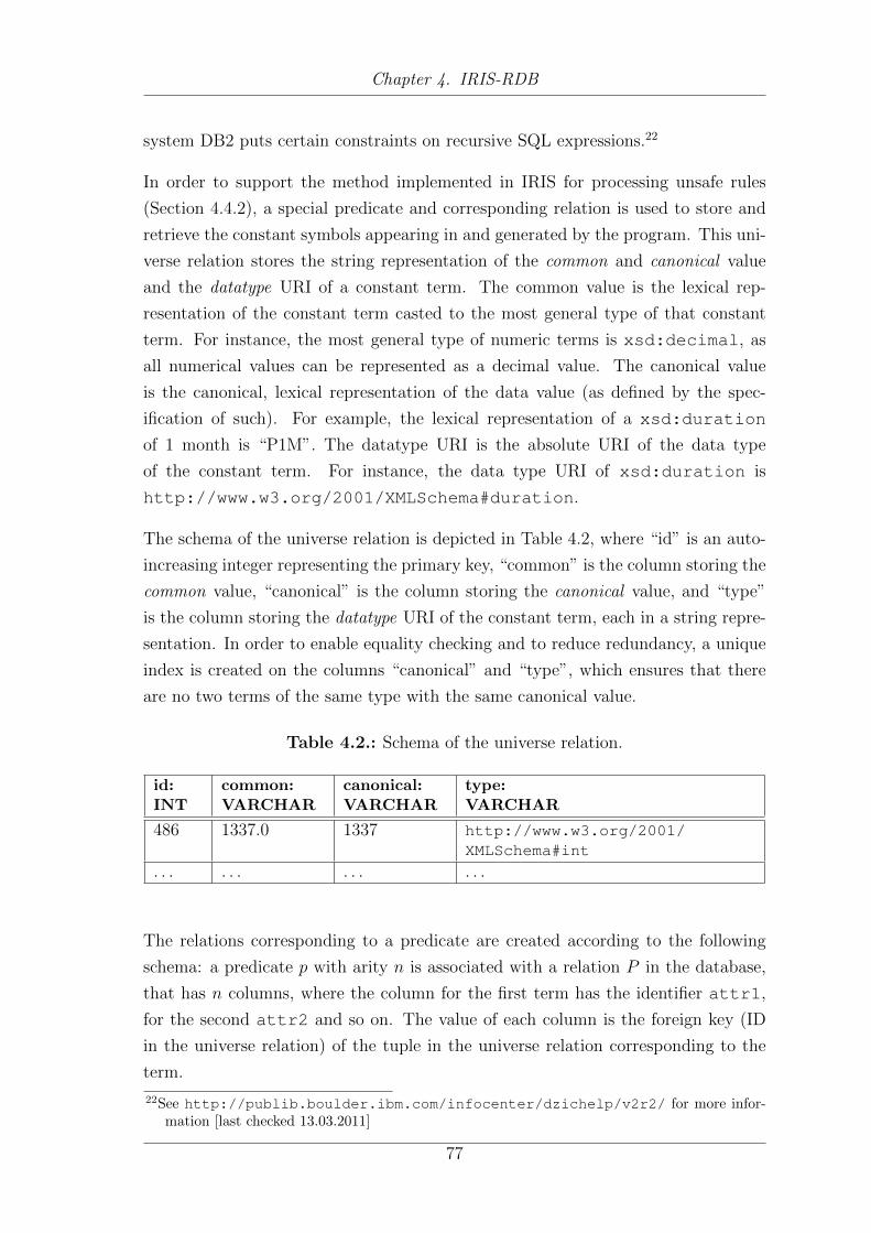
Chapter 4. IRIS-RDB
system DB2 puts certain constraints on recursive SQL expressions.22
In order to support the method implemented in IRIS for processing unsafe rules
(Section 4.4.2), a special predicate and corresponding relation is used to store and
retrieve the constant symbols appearing in and generated by the program. This uni-
verse relation stores the string representation of the common and canonical value
and the datatype URI of a constant term. The common value is the lexical rep-
resentation of the constant term casted to the most general type of that constant
term. For instance, the most general type of numeric terms is xsd:decimal, as
all numerical values can be represented as a decimal value. The canonical value
is the canonical, lexical representation of the data value (as defined by the spec-
ification of such). For example, the lexical representation of a xsd:duration
of 1 month is “P1M”. The datatype URI is the absolute URI of the data type
of the constant term. For instance, the data type URI of xsd:duration is
http://www.w3.org/2001/XMLSchema#duration.
The schema of the universe relation is depicted in Table 4.2, where “id” is an auto-
increasing integer representing the primary key, “common” is the column storing the
common value, “canonical” is the column storing the canonical value, and “type”
is the column storing the datatype URI of the constant term, each in a string repre-
sentation. In order to enable equality checking and to reduce redundancy, a unique
index is created on the columns “canonical” and “type”, which ensures that there
are no two terms of the same type with the same canonical value.
Table 4.2.: Schema of the universe relation.
id:INT
common:VARCHAR
canonical:VARCHAR
type:VARCHAR
486 1337.0 1337 http://www.w3.org/2001/XMLSchema#int
. . . . . . . . . . . .
The relations corresponding to a predicate are created according to the following
schema: a predicate p with arity n is associated with a relation P in the database,
that has n columns, where the column for the first term has the identifier attr1,
for the second attr2 and so on. The value of each column is the foreign key (ID
in the universe relation) of the tuple in the universe relation corresponding to the
term.
22See http://publib.boulder.ibm.com/infocenter/dzichelp/v2r2/ for more infor-mation [last checked 13.03.2011]
77

Chapter 4. IRIS-RDB
This enables two different implementations of joins. The first solution – which is
actually the one currently used by IRIS-RDB – joins two tables on the integers
values of the attribute columns, which means that those tuples are joined, where
the attribute at the specified position has the same canonical value and data type
URI. The second method uses the normalized string values of the attributes that is
being joined on. This however would require additional joins to the universe relation
when joining two relations and, therefore, may significantly reduce performance.
4.5.2. The Relation Defined By a Rule Body
A rule may be evaluated by computing a relation for the rule body using relational
algebra operations. A modified version of the algorithm defined in [35, page 109]
(Algorithm A.1 in Appendix A) has been implemented. This version of the algo-
rithm requires the literals of the rule body to be re-ordered such that all but the
allowed unbound variables of a built-in are already bound by a preceding literal. The
symbols π and σ refer to the standard relational operations projection and selection,
respectively, as shown, for instance, in [35, page 56].
Algorithm: Computing the Relation for a Rule Body.
Input: The body of a Datalog rule r, which consists of subgoals S1, . . . , Sn contain-
ing variables X1, . . . , Xm. For each Si = pi(ci1 , ..., ciki ) with a non-built-in predicate,
there is a relation Ri already computed, where the c’s are arguments, either variables
or constants.
Output: An expression of relational algebra, which we call
EVAL-RULE(r, R1, ..., Rn)
that computes from the relations R1, . . . , Rn a relation R(X1, . . . , Xm) with all and
only the tuples (a1, ..., am) such that, when we substitute aj for each Xj, 1 ≤ j ≤ k,
all the subgoals S1, . . . , Sn are made true.
Method: The expression is constructed by the following steps.
1 A := ∅2 O := ∅3 for i := 1 to n do
4 Let (s1, ..., sl) be the arguments of Si, where the s’s are either
variables or constants.
78

Chapter 4. IRIS-RDB
5 if Si is positive then
6 if pi is not a built-in predicate then
7 Let T be the expression σF (Ri). F is the conjunction of the
following conditions:
8 1. If position k of Si has constant a, then F has the term
$k = a
9 2. If position k and l of Si both contain the same variable,
then F has the term $k = $l
10 if A 6= ∅ then
11 Let Y1, . . . , Yr be the variables occurring in O, where each
variable appears only once in the list.
12 Let G be the conjunction of the following conditions:
13 1. If some Y is also in (s1, ..., sl) and let a be the position of
Y in O and b be the position of Y in (s1, ..., sl) then G
has the term $a = $b
14 If G is not empty then let A be the expression σF (A× T )
otherwise let A be the expression (A× T ).
15 else
16 Let A be T.
17 fi
18 else
19 Let Q be a new relation in the database with arity c+ d, where c
is the arity of A and d is the arity of the built-in
predicate. Here A is not empty, as the rule is safe.
20 Let Y1, . . . , Yr be the variables occurring in O, where each variable
appears only once in the list.
21 Let F be the conjunction of the following conditions:
22 1. If some Y is also in (s1, . . . , sl) and let a be the position of
Y in O and b be the position of Y in (s1, ..., sl), then F has
the term $a = $b
23 Let T be σF (A) and let (a1, . . . , ac) be the tuples from T and let
(b1, . . . , bd) be the tuples from the result of the evaluation of
the built-in where some of b1, . . . , bd are the input extracted
from (a1, . . . , ac) and some are the output terms of the built-in.
Add all tuples (a1, . . . , ac, b1, . . . , bd) to Q for whose (b1, . . . , bd) the
built-in holds.
24 Let A be Q.
25 fi
26 Let O be the concatenation of O and (s1, ..., sl).
27 else
28 if pi is not a built-in predicate then
29 Let U be A.
30 Let T be the expression σF (Ri), where F is the conjunction of the
following conditions:
31 1. If position k of Si has constant a, then F has the term
$k = a
79

Chapter 4. IRIS-RDB
32 2. If position k and l of Si both contain the same variable,
then F has the term $k = $l
33 if A 6= ∅ then
34 Let Y1, . . . , Yr be the variables occurring in O, where each
variable appears only once in the list.
35 Let G be the conjunction of the following conditions:
36 1. If some Y is also in (s1, ..., sl) and let a be the position of
Y in (s1, ..., sl) and b be the position of Y in Y1, . . . , Yr then
G has the term $a 6= $b
37 Let A be the expression π1,...,cσG(U × T ), where c is the arity of
U.
38 fi
39 else
40 Let Q be a new relation in the database with arity c, where c is
the arity of A.
41 Let Y1, ..., Yr be the variables occurring in O, where each variable
appears only once in the list.
42 Let F be the conjunction of the following conditions:
43 1. If some Y is also in (s1, ..., sl) and let a be the position of Y
in O and b be the position of Y in (s1, ..., sl), then F has
the term $a = $b
44 Let T be σF (A) and let (a1, ..., ac) be the tuples from T and let
(b1, ..., bd) be the tuples from the result of the evaluation of
the built-in where some of b1, ..., bd are the input (extracted
from (a1, ..., ac)) and some are the output terms of the built-in.
Add all tuples (a1, ..., ac) to Q for which the built-in does not
hold.
45 Let A be Q.
46 fi
47 fi
48 end
49 Let EVAL-RULE(r,R1, ..., Rn) be πq1,...,qmA where qi is the position of variable
Xi in O.
The algorithm iterates over all literals in the rule body and creates a view on the
relation of the current literal which filters the tuples of the relation according to the
constants and variables appearing in the literal. Then, the algorithm joins this view
with the relation created for the previous literals, if existing. The indices for the join
are determined based on the variables occurring in the literal and those appearing
in the tuple O, which represents the concatenation of (s1, ..., sl) of all the previous
literals. In the case of a built-in, the algorithm uses the values from the relation of
the previous literals or the constant values of the built-in predicate itself in order
to evaluate the built-in. A new relation is created, which stores all the tuples for
which the evaluation of the built-in is valid. Finally, the relations are joined on the
80
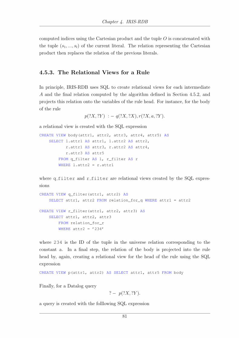
Chapter 4. IRIS-RDB
computed indices using the Cartesian product and the tuple O is concatenated with
the tuple (s1, ..., sl) of the current literal. The relation representing the Cartesian
product then replaces the relation of the previous literals.
4.5.3. The Relational Views for a Rule
In principle, IRIS-RDB uses SQL to create relational views for each intermediate
A and the final relation computed by the algorithm defined in Section 4.5.2, and
projects this relation onto the variables of the rule head. For instance, for the body
of the rule
p(?X, ?Y ) : − q(?X, ?X), r(?X, a, ?Y ).
a relational view is created with the SQL expression
CREATE VIEW body(attr1, attr2, attr3, attr4, attr5) AS
SELECT l.attr1 AS attr1, l.attr2 AS attr2,
r.attr1 AS attr3, r.attr2 AS attr4,
r.attr3 AS attr5
FROM q_filter AS l, r_filter AS r
WHERE l.attr2 = r.attr1
where q filter and r filter are relational views created by the SQL expres-
sions
CREATE VIEW q_filter(attr1, attr2) AS
SELECT attr1, attr2 FROM relation_for_q WHERE attr1 = attr2
CREATE VIEW r_filter(attr1, attr2, attr3) AS
SELECT attr1, attr2, attr3
FROM relation_for_r
WHERE attr2 = ’234’
where 234 is the ID of the tuple in the universe relation corresponding to the
constant a. In a final step, the relation of the body is projected into the rule
head by, again, creating a relational view for the head of the rule using the SQL
expression
CREATE VIEW p(attr1, attr2) AS SELECT attr1, attr5 FROM body
Finally, for a Datalog query
?− p(?X, ?Y ).
a query is created with the folllowing SQL expression
81

Chapter 4. IRIS-RDB
SELECT attr1, attr2 FROM p
The usage of relational view enables the optimizer of the database system to find a
well-performing execution plan for the final SQL query.
82

5
Evaluation
The evaluation of the two software components developed in the course of this master
thesis is carried out separately. Section 5.1 describes the evaluation of the RIF4J
reasoning engine, which tests the conformance of the two reasoning components
based on IRIS and IRIS-RDB. The evaluation of IRIS-RDB, described in Section
5.2, focuses on the comparison of the original IRIS with IRIS-RDB with respect to
the performance and, more importantly, to the scalability of the system.
5.1. RIF4J
This section shows the results of the evaluation of the prototypical reasoners using
the RIF-BLD (positive and negative) entailment test cases of the RIF-BLD test
suite v1.22 described in [32] and deployed on the repository for RIF Test Cases.23
According to [32, Section 1.1], the tests are designed to:
• Aid in conformance evaluation by providing evidence that the specification
has been implemented.
• Provide generally broad coverage of the language features.
• Focus on non-obvious features and behavior, and hard to implement features,
since these types of tests are more likely to uncover problems in implementa-
tions.
• Pinpoint omissions that can be corrected.
23Repository for RIF Test Cases, http://www.w3.org/2005/rules/test/repository/[last checked 10.03.2011]
83

Chapter 5. Evaluation
• Illustrate the use and meaning of language features.
It is important to note that the RIF-BLD test suite does not cover all requirements
for a conformant RIF-BLD system (in the following also called RIF-BLD processor).
However, failure to pass specific tests in the suite indicates that the implementation
does not meet the relevant specification. Despite its rather limited size the test suite
is a valuable utility for the evaluation of the RIF-BLD conformance of a system.
5.1.1. Positive Entailment Test
The positive entailment tests of the RIF-BLD test suite are used to validate the
computation of the logical entailment relation of a RIF-BLD processor. Each of the
14 test cases consists of a RIF-BLD document formula representing the premise,
a condition formula24 representing the conclusion and optionally one or more doc-
uments in the imports closure of the premise document. The goal of a positive
entailment test is to check if the system is able to show that the premise entails
the conclusion. According to [32, Section 3.3.1], a conformant RIF consumer should
report that the conclusion is entailed by the premises, should not report that the
answer is undecided, and must not report that the conclusion is not entailed by the
premises.
Table 5.1 shows the results of the positive entailment tests against the RIF-BLD
processors based on the IRIS and IRIS-RDB Datalog reasoners. Correct results
are denoted with the term “True” and are highlighted with a green background
color, whereas, “False” indicates incorrect results, which are highlighted with a red
background color. The orange background color indicates, that the systems should
actually reject the premise or the conclusion formula, since it contains features
that the system does not support.25 In the following the failing test cases and the
respective results of the evaluation are described in more detail.
• Arbitrary Entailment: In this test case, the premise represents an incon-
sistent formula, as it asserts equality between the strings ”a” and ”b”, which
are different according to [6]. According to the definition of RIF-BLD logical
entailment, an inconsistent formula entails everything. However, per initial
design decision there is no concept of inconsistency in IRIS and IRIS-RDB.
Essentially, it can only be shown if an atomic formula or a conjunction of such
24See Definition 2.3.425See Section 2.3.2.3
84

Chapter 5. Evaluation
Table 5.1.: Results of positive entailment tests.
Test case IRIS IRIS-RDB
Arbitrary Entailment False* False*Chaining strategy numeric-add 2 True TrueChaining strategy numeric-subtract 1 False FalseClass Membership True TrueClassification-inheritance True TrueElementEqualityFromListEquality True TrueEntailEverything False* False*Equality in conclusion 1 True TrueEquality in conclusion 2 True False*Equality in conclusion 3 False False*Equality in condition False FalseFactorial Functional False False*Factorial Relational False FalseInconsistent Entailment False FalseIndividual-Data Separation Inconsistency False FalseIRI from IRI True TrueListConstantEquality True False*ListEqualityFromElementEquality True False*ListLiteralEquality False* False*Multiple IRIs from String True TrueMultiple Strings From IRI True TrueNamed Arguments True TrueRDF Combination Member 1 True TrueRDF Combination SubClas 4 False FalseRDF Combination SubClass 6 True TrueYoung Parent Discount 1 True True
* Contains unsupported features.
is entailed by the least Herbrand model computed by IRIS, in the sense that
the ground instantiations of the formulas are elements of the model. In other
words, in IRIS there only exists the concept of an empty model but not that
of “no model”.
• Chaining strategy numeric-subtract 1: Both IRIS and IRIS-RDB fail to
show the entailment of the conclusion formula, as the Datalog program evalua-
tion fails. The reason for this is that IRIS and IRIS-RDB both use a bottom-up
evaluation technique to compute a least Herbrand model for the premise doc-
ument, which is, however, infinite, since Datalog equivalent for the universal
rule in the premise is unsafe (variable ?X is not limited).
85

Chapter 5. Evaluation
• ElementEqualityFromListEquality: For IRIS-RDB, the reason for the
failure of this test (and also of the other list related tests) is that it currently
does not support list terms (Section 4.3).
• EntailEverything: IRIS and IRIS-RDB do not support universal facts, there-
fore, the test fails. The reason for this is, again, that in IRIS it can only be
shown if an atomic formula or a conjunction of such is entailed by the least
Herbrand model.
• Equality in conclusion 2: This test fails for IRIS-RDB, as the system does
not support function symbols.
• Equality in conclusion 3: For IRIS, the test fails since functions symbols
are not correctly substituted when deeply nested in other function symbols.
IRIS-RDB fails to entail the conclusion, as it does not support function sym-
bols.
• Equality in condition: In this test case, the computation of the least Her-
brand model does not succeed, since the Datalog program corresponding to
the premise document produces an infinite model due to the unsafeness of the
Datalog rule for the premise formula (variable ?X is not limited).
• Factorial Functional: In this test case, a function symbol appears in a built-
in function of the premise formula, which is, however, not allowed in IRIS.
IRIS-RDB fails to entail the conclusion, as it does not support function sym-
bols.
• Factorial Relational: Similar as in the test Chaining strategy numeric- sub-
tract 1, the computation of the least Herbrand model does not terminate, as
the Datalog rule for the formula in the premise document is unsafe (variables
?N and ?F are not limited).
• Inconsistent Entailment: This test case is very similar to the Arbitrary En-
tailment test and fails for the same reasons.
• Individual-Data Separation Inconsistency: The premise document of
this test case imports a document under the OWL-Direct [22] profile, which is
not supported by RIF4J and the included reasoning components.
• ListConstantEquality: This test case fails for IRIS-RDB as it does not
support list terms.
86

Chapter 5. Evaluation
• ListEqualityFromElementEquality: This test case fails for IRIS-RDB as
it does not support list terms.
• ListLiteralEquality: The premise document of this test case entails false-
hood (written as Or()), which can not be expressed neither in IRIS nor in
IRIS-RDB.
• RDF Combination SubClass 4: In this test case, the premise document
imports a document under the RDFS [22] profile, which is not supported by
RIF4J and the included reasoning components.
5.1.2. Negative Entailment Test
Each of the 5 negative entailment tests consists of a RIF-BLD document formula
representing the premise, a condition formula representing the conclusion and op-
tionally one or more documents in the imports closure of the premise document.
The goal of a negative entailment test, is to check if the system is able to show
that the premise does not entail the conclusion. According to [32, Section 3.3.2], a
conformant RIF consumer should report that the conclusion is not entailed by the
premises, should not report that the answer is undecided, and must not report that
the conclusion is entailed by the premises.
Table 5.2 shows the results of the negative entailment tests against the RIF-BLD
processors based on the IRIS and IRIS-RDB Datalog reasoners. Correct results
are denoted with the term “False” and are highlighted with a green background
color, whereas, “True” indicates incorrect results, which are highlighted with a red
background color. The orange background color indicates, that the systems should
actually reject the premise or the conclusion formula, since it contains features that
the system does not support. In the following the failing test cases and the respective
results of the evaluation are described in more detail.
• OpenLists: The reason for the failure of this test case is that IRIS does
only support closed lists, and, therefore, open lists are transformed into closed
lists with only non-list terms as elements. Thus, the list in the premise is
converted to the same as the one in the conclusion, and, therefore, the result
of the evaluation is true and the test fails.
87

Chapter 5. Evaluation
Table 5.2.: Results of negative entailment tests.
Test case IRIS IRIS-RDB
Classification non-inheritance False FalseNamed Argument Uniterms non-polymorphic False FalseOpenLists True False*RDF Combination SubClass 3 False FalseRDF Combination SubClass 5 False False
* Contains unsupported features.
5.1.3. Evaluation Conclusion
The results of the positive and negative entailment tests show that the prototypical
reasoners based on IRIS are strictly speaking no conformant RIF-BLD consumers
(Definition 2.3.17), as for some tests cases the systems fail to compute the correct
result for the entailment relation.
As can be observed from the results in Section 5.1.1 and Section 5.1.2, the reason for
the failure of some test cases are fundamental: For instance, the reasoners lack the
concept of falsehood or “no model”, which on the one hand prevents that any formula
can be entailed from a contradiction, and on the other hand, that a contradiction
entails falsehood. Furthermore, the bottom-up evaluation technique implemented in
both systems causes some of the test cases to fail (due to an infinite model), where
top-down methods would succeed in computing the correct result.
Nevertheless, the reasoners cover many of the features required by RIF-BLD, that
may suffice for reasoning on a multitude of knowledge bases. In particular, the
systems support all datatypes and built-ins required by RIF-DTB and equality in
the rule head. Preliminary support for RDF importing is implemented allowing
(simple) reasoning over RDF data using the formalism of RIF-BLD. Additionally,
the reasoner based on IRIS allows function symbols and list terms.
5.2. IRIS-RDB
IRIS-RDB has been developed with the goal to have a more scalable Datalog rea-
soner, which can process Datalog programs that contain and produce facts that do
not fit in the memory of a single computer. The evaluation focuses on the compari-
88

Chapter 5. Evaluation
son of the original IRIS with IRIS-RDB with respect to the performance and, more
importantly, to the scalability of the system.
All test results were produced using the rule-filtering and Magic Sets optimization
techniques and were run on a system with:
• Intel R© CoreTM i7-620M 2x 2.66GHz,
• Windows 7 (64-bit),
• 4 Gbyte DDR2 RAM,
• Oracle Java SE Development Kit (JDK) 6 Update 23 (32-bit).
Similar as for the OpenRuleBench, the focus of this evaluation was to measure the
time to do inference rather than loading the test data sets. Thus, we only measured
the time it took to evaluate a query, and did not consider the loading of the facts
into the database. If not stated otherwise, the results in the tables below show the
times measured in seconds.
5.2.1. OpenRuleBench
The scalability tests were taken from the OpenRuleBench [26] test suite, in partic-
ular, the test cases of the large join tests category, which includes large database
joins, LUBM-derived tests, the Mondial and the DBLP test. In the detailed report
of the OpenRuleBench [27] it has been observed that IRIS could not handle any of
the large join tests, due to a timeout. Therefore, these test cases seemed to be a
suitable candidate to check if the IRIS-RDB system meets the stated expectations.
Unfortunately, only the Join1, Join2 and DBLP tests could be run, as the LUBM-
derived tests were not available in an IRIS compatible format, and the Mondial tests
contained function symbols, which are not supported by IRIS-RDB.
Unlike the OpenRuleBench we did not use a timeout, which determined the max-
imum allowed time to run an evaluation, but waited until the system produced a
result or until an error occurred. In the tables below, “Error” means, that the sys-
tem produced an OutOfMemoryError after some time, even if we assigned the
maximum of 1536 megabyte of memory to the Java virtual machine.
89

Chapter 5. Evaluation
5.2.1.1. Join1
The Join1 test has a form of a non-recursive tree of binary joins, which is expressed
using the rules shown in Listing 5.1.
Listing 5.1: Rules for Join1.
1 a(?X, ?Y) :- b1(?X, ?Z), b2(?Z, ?Y).
2 b1(?X, ?Y) :- c1(?X, ?Z), c2(?Z, ?Y).
3 b2(?X, ?Y) :- c3(?X, ?Z), c4(?Z, ?Y).
4 c1(?X, ?Y) :- d1(?X, ?Z), d2(?Z, ?Y).
The relations for the predicates c2, c3, c4, d1, and d2 were randomly generated.
OpenRuleBench provides three datasets: data0 with 50 000, data1 with 250 000
and data2 with 1 250 000 tuples. In our evaluation we only used the datasets data0
and data1 as the IRIS parser did not manage to process data2 containing 1 250 000
tuples.
The test further defines nine queries on the predicates a, b1 and b2. There are
three queries for each predicate where one query has no variable binding, one has
a binding on the first variable and one has a binding on the second variable. The
queries are shown in Listing 5.2, where each line in the listing represents a single
test.
Listing 5.2: Queries for Join1.
1 ?- a(?X, ?Y).
2 ?- b1(?X, ?Y).
3 ?- b2(?X, ?Y).
4
5 ?- a(1, ?Y).
6 ?- b1(1, ?Y).
7 ?- b1(1, ?Y).
8
9 ?- a(?X, 1).
10 ?- b1(?X, 1).
11 ?- b2(?X, 1).
Table 5.3 shows the results of the Join1 test with unbound variables in the query.
As known, the original IRIS could not compute the result for query “a” due to the
OutOfMemoryError. Interestingly, for data0 we succeeded in computing results
for the other two queries, unlike in the evaluation conducted by OpenRuleBench
authors, where IRIS did not manage to evaluate any of the programs. This might
be the case, since the OpenRuleBench authors only assigned 512 megabyte of mem-
90

Chapter 5. Evaluation
ory to the Java virtual machine running the programs, whereas we assigned 1536
megabyte of memory. This also applies for the Join2 test in Section 5.2.1.2.
Table 5.3.: Times for Join1, no query bindings.
data0 data1a b1 b2 a b1 b2
IRIS-RDB 1068.875 67.726 7.112 16685.639 474.931 74.71IRIS Error 19.069 1.417 Error Error 45.16
Table 5.4 shows the results of the Join1 test with a binding on the first variable.
In this test, both systems take heavy advantage of the Magic Sets optimization in
order to rewrite the program in a way such that the data handled in the process
of evaluation is limited by the variable bindings in the query. Thus, the evaluation
times are significantly lower than in the test above. For data0, IRIS performs better
than IRIS-RDB in all three tests, showing a significant difference for the query on
predicate a. For data1 IRIS did not manage to compute the first two queries due to
an OutOfMemoryError. Interestingly, it can be observed, that the performance
difference for query “b2” is less significant than for data0. We assume that for larger
fact bases the drawback of hard-disk access may be amortized by the set-oriented
techniques used by the database system.
Table 5.4.: Times for Join1 with first argument bound.
data0 data1a b1 b2 a b1 b2
IRIS-RDB 13.275 0.475 0.178 186.372 0.749 0.187IRIS 1.332 0.135 0.112 53.711 0.593 0.172
Table 5.5 shows the results of the final Join1 test where the second variable is bound.
In this test, IRIS performs significantly better than IRIS-RDB on all three queries.
For query “a” on data1 IRIS did not manage to evaluate the program.
Table 5.5.: Times for Join1 with second argument bound.
data0 data1a b1 b2 a b1 b2
IRIS-RDB 164.119 21.497 1.061 735.923 454.904 18.611IRIS 34.725 1.404 0.063 Error 62.681 0.625
91

Chapter 5. Evaluation
5.2.1.2. Join2
The Join2 test defines the rules and queries shown in Listing 5.3. The facts for the
program consist of the tuples p(abcd0), ..., p(abcd18). The program produces a large
intermediate result, but only a small set of answers for the query ?− q(?X).
Listing 5.3: Rules for Join2.
1 ra(?A, ?B, ?C, ?D, ?E) :- p(?A), p(?B), p(?C), p(?D), p(?E).
2 rb(?A, ?B, ?C, ?D, ?E) :- p(?A), p(?B), p(?C), p(?D), p(?E).
3 r(?A, ?B, ?C, ?D, ?E) :- ra(?A, ?B, ?C, ?D, ?E),
4 rb(?A, ?B, ?C, ?D, ?E).
5 q(?A) :- r(?A, ?B, ?C, ?D, ?E).
6 q(?B) :- r(?A, ?B, ?C, ?D, ?E).
7 q(?C) :- r(?A, ?B, ?C, ?D, ?E).
8 q(?D) :- r(?A, ?B, ?C, ?D, ?E).
9 q(?E) :- r(?A, ?B, ?C, ?D, ?E).
Table 5.6 shows the results of the Join2 test. IRIS did not manage to evaluate the
program due to an OutOfMemoryError.
Table 5.6.: Times for Join2.
q
IRIS-RDB 1773.478IRIS Error
5.2.1.3. DBLP
The DBLP test contains a subset of the Digital Bibliography & Library Project
(DBLP) database consisting of information about publications in the field of com-
puter science. The test data set defines a single relation with approximately 2 500
000 facts (corresponding to 2 500 000 tuples) about 200 000 publications. The DBLP
test defines the rules and queries shown in Listing 5.4 and Listing 5.5, where the
query seeks the ID, title, authors, year and month for all publications.
Listing 5.4: Rules for DBLP.
1 query(Id,T,A,Y,M) :- att(Id,title,T), att(Id,year,Y),
2 att(Id,author,A), att(Id,month,M).
Listing 5.5: Queries for DBLP.
1 ?- queryrule(?X,?T,?Y,?A,?M).
92

Chapter 5. Evaluation
Table 5.7 shows the results of the DBLP test. IRIS did not manage to evaluate the
program due to an OutOfMemoryError.
Table 5.7.: Times for DBLP.
queryrule
IRIS-RDB 2.557IRIS Error
5.2.1.4. Built-in Predicates
In order to test the performance of Datalog programs with built-in predicates, we
have run the program shown in Listing B.3 in Appendix B, where we have varied
the number that limits the range of the variable X and, therefore, determines the
number of recursive calls of the rule on line 2. Surprisingly, IRIS-RDB performs
almost as well as the original IRIS. We expected that, due to the one-tuple-at-a-
time iteration, and the continuous hard disk access that is required when evaluating
rules with built-in predicates, the performance of IRIS-RDB would be significantly
worse than the in-memory evaluation of IRIS.
Table 5.8 depicts the results of the evaluations, where the number in parentheses
shows the number of tuples in the output relation of the predicate path.
Table 5.8.: Times for program with built-in predicates.
200 (20503) 400 (80601) 800 (321201) 1000 (501501)
IRIS 14.365 100.216 1056.399 2439.453IRIS-RDB 9.92 86.623 825.255 1897.620
5.2.2. Evaluation Conclusion
The results show that IRIS-RDB is able to evaluate Datalog programs for which
the original in-memory implementation fails to compute a result. In particular,
the system supports knowledge bases with millions of input facts, whose evaluation
results in the creation of a multitude of intermediate facts. However, the results also
outline that IRIS performs better than IRIS-RDB in those tests that it manages to
process, i.e., knowledge bases that fit into the memory of a single computer. The
93

Chapter 5. Evaluation
reason for this may be that IRIS-RDB requires continuous hard disk access, whereas,
IRIS processes everything in-memory. Furthermore, in each run of the semi-naive
evaluation, the system copies each incremental relation (∆Pi in Algorithm A.3)
to a dedicated relation in the database, which may also have an influence on the
performance, especially for large and numerous intermediate relations.
We also presume that the performance of IRIS-RDB could be increased by reducing
the tuple size of the intermediate relations and by optimizing the SQL expressions,
for instance, by changing the order of the joins, such that relations with the smallest
size are joined first, which in turn reduces the size of intermediate relations. The
performance could further be improved by an automatic analysis to establish ap-
propriate indices on the database relations to speed up rule and query evaluation
time. In order to support more expressive programs, the list of features of IRIS-
RDB could be extended in order to support knowledge bases with rules containing
function symbols and list terms.
An advantage of using a relational database system as underlying engine for eval-
uating Datalog programs is that the system may benefit of the performance opti-
mizations of future versions of the DBMS. Additionally, the system could be used
with more specialized or distributed database system that may scale to the size of
billions of tuples.
94

6
Conclusion
This master thesis has addressed the challenge of designing and implementing a
RIF-BLD conformant reasoning engine based on a Datalog system in general, and
IRIS in particular. In the following, a recapitulation of the established contributions
and an outlook to further research topics in the area is given.
6.1. Contribution
RIF4J has been developed as a reasoning engine that allows for the programmatic
processing of knowledge represented in the Basic Logic Dialect (BLD) of RIF, and
enables the reasoning upon this knowledge using the Datalog systems IRIS. This
has been realized through a translation of RIF-BLD formulas to equivalent Datalog
programs. In order to support data that exceeds the limits of a single computer’s
memory, IRIS-RDB has been developed as an extension of IRIS that leverages the
close relationship of Datalog and relational algebra, and implements an evaluation
strategy based on a relational database system.
RIF4J provides an object model capable of representing RIF-BLD documents in
the Java programming language. The system is designed with flexibility and ex-
tendability in mind encouraging the implementation of additional algorithms and
utilities on top of the object model. The incorporation of the visitor pattern enables
to easily implement new functionality using the object model of RIF4J. Examples of
additional features are the integrated utilities for parsing and serializing RIF-BLD
documents.
RIF-BLD reasoning with Datalog has been realized by a semantic-preserving
95

Chapter 6. Conclusion
translation from RIF-BLD to Datalog such that the resulting Datalog programs
and queries can be evaluated using a Datalog engine. A formal definition of this
translation has been specified and an implementation thereof is provided based on
the RIF4J and IRIS object models. Two prototype implementations of RIF-BLD
reasoners based on the Datalog engines IRIS and IRIS-RDB have been developed,
where both systems take advantage of the translation implementation in order to
carry out RIF-BLD reasoning tasks. To test the conformance to RIF-BLD, both
prototypes have been evaluated against the RIF-BLD test suite provided by the
RIF working group. It has been shown that the prototypes cover important features
of the RIF-BLD formalism. However, fundamental initial design decisions in IRIS
prohibit the successful evaluation of those test cases, which test the entailment
of falsehood or validate that falsehood entails everything. Furthermore, some test
cases fail due to the bottom-up evaluation technique implemented in IRIS and IRIS-
RDB.
IRIS-RDB has been developed as an extension of IRIS that uses a relational
database as an underlying system to evaluate Datalog programs. The goal of IRIS-
RDB is to have a more scalable reasoning engine that is able to process knowledge
bases that exceed the limits of a single computer’s memory. IRIS-RDB can evalu-
ate safe or unsafe Datalog programs containing rules with equality in the head and
negation as failure. It supports all datatypes and built-ins required to be imple-
mented in any RIF conformant system. It has been shown that the system is able
to evaluate Datalog programs for which the original IRIS fails to compute a result
due to the limits on the data it can process in memory. However, this increased
degree of scalability comes at the cost of reduced performance on programs where
this does not apply. For instance, the OpenRuleBench tests have shown that the
original IRIS performs better in those tests that can be evaluated in-memory.
6.2. Future Work
Even though RIF4J together with IRIS and IRIS-RDB have shown to capture most
of the features required for RIF-BLD reasoning, the systems should still be improved
in order to be fully standards-conformant RIF-BLD reasoners. There are deficien-
cies that cause the IRIS and IRIS-RDB based reasoners to fail some test cases in the
RIF-BLD test suite. In particular, the Datalog systems are not able to represent
inconsistencies or falsehood, nor is it possible to define and reason about universal
facts. Therefore, the evaluation strategies implemented in the Datalog engines need
96

Chapter 6. Conclusion
to be extended to enable the identification and representation of inconsistent knowl-
edge bases and universal facts. To allow for RIF-BLD reasoning over knowledge
bases under the RDF(S) and OWL semantics, support for the import of documents
under the RDF(S) and OWL profiles defined in [22] needs to be implemented. In
the case of the IRIS-RDB based reasoner, support for list terms and an evaluation
strategy supporting function symbols need to be developed, in order to support
knowledge bases containing such features.
As far as the IRIS extension IRIS-RDB is concerned, the Datalog system has shown
to be capable of reasoning over knowledge bases containing several millions of facts,
which the original IRIS system fails to process, due to the in-memory data manage-
ment. Still, further research and development is required to support the handling
and processing of data at Web-scale, i.e., to efficiently reason over knowledge bases
consisting of billions of facts. As a starting point, the usage of distributed relational
database systems together with the relational algebra based evaluation strategy im-
plemented in the course of this thesis could be investigated to run the evaluation on
a distributed architecture. In that way the reasoning framework can reach out to
the data sets of Linked Data that encompass billions of triples.
Further, an evaluation of current NoSQL (Not Only SQL) systems would be inter-
esting, in order to determine the most appropriate back-end with respect to Datalog
suitability, data scalability and reasoning performance over large fact bases. For in-
stance, in [16] a parallelized Datalog system is currently under development, which
leverages techniques such as data and rule partitioning and map-reduce-style pro-
gramming models using the Apache Hadoop framework.26
26Apache Hadoop, http://hadoop.apache.org/ [19.03.2011]
97

A
Algorithms
98

Appendix A. Algorithms
Algorithm A.1 Computing the Relation for a Rule Body Using Relational AlgebraOperations
Input: The body of a Datalog rule r, which we shall assume consists of subgoalsS1, . . . , Sn involving variables X1, . . . , Xm. For each Si = pi(Ai1, . . . , Aiki) withan ordinary predicate, there is a relation R already computed, where the A′s arearguments, either variables or constants.Output: An expression of relational algebra, which we call
EVAL-RULE(r, R1, . . . , Rn)
that computes from relations R1, . . . , Rn a relation R(X1, . . . , Xm) with all and onlythe tuples (a1, . . . , am) such that, when we substitute aj for Xj, 1 ≤ j ≤ m all thesubgoals S1, . . . , Sn are made true. Note that not all n relations may be presents,as some of the subgoals may have built-ins predicates. We later use the relationalexpressions of rules to successively build up the least Herbrand model for a Datalogprogram.Method: The expression is constructed by the following steps.
1. For each ordinary Si, let Qi be the expression πVi(σFi
(Ri)).Here, Vi is a set of components including, for each variable X that appearsamong the arguments of Si, exactly one component where X appears. Also,Fi is the conjunction (logical AND) of the following conditions.
a) If position k of Si has a constant a, then Fi has the term $k = a.
b) If position k and l of Si both contain the same variable, then Fi has theterm $k = $l.
As a special case, if Si is such that there are no terms in Fi, e.g., Si = p(X, Y ),then take Fi to be the identically true condition, so Qi = Ri.
2. For each variable X not found among the ordinary subgoals, compute anexpression DX that produces a unary relation containing all the values of ruler. Since r is safe, there is some variable Y to which X is equated through asequence of one or more = subgoals, and Y is limited either by being equated tosome constant a in a subgoal or by being an argument of an ordinary subgoal.
a) If Y = a is a subgoal, then let DX be the constant expression {a}.b) If Y appears as the jth component of the ordinary subgoal Si, let DX be
πj(Ri).
3. Let E be the natural join of all the Qi’s defined in (1) and the DX ’s defined in(2). In this join, we regard Qi as a relation whose attributes are the variablesappearing in Si, and we regard DX as a relation with attribute X.
4. Let EVAL-RULE(r, R1, . . . , Rn) be σF (E), where F is the conjunction of XθYfor each built-in subgoal XθY appearing among p1, . . . , Pn and E is the ex-pression constructed in (3). If there are no built-in subgoals, then the desiredexpression is just E.
99
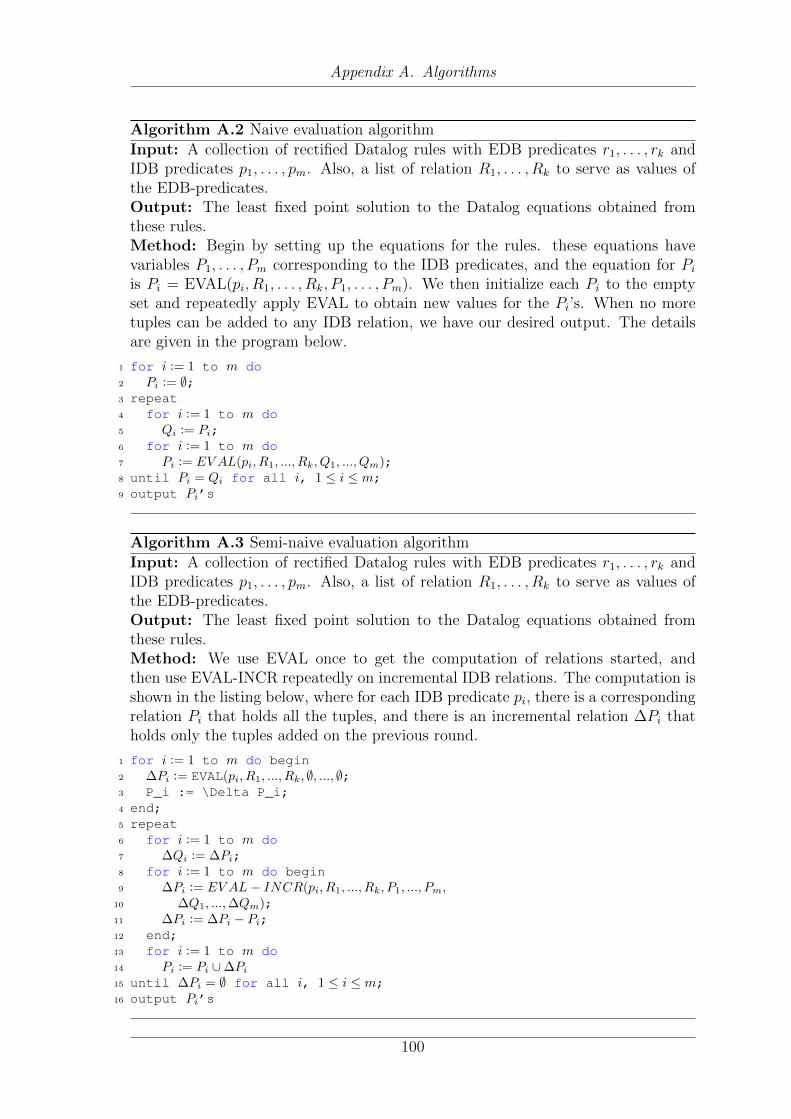
Appendix A. Algorithms
Algorithm A.2 Naive evaluation algorithm
Input: A collection of rectified Datalog rules with EDB predicates r1, . . . , rk andIDB predicates p1, . . . , pm. Also, a list of relation R1, . . . , Rk to serve as values ofthe EDB-predicates.Output: The least fixed point solution to the Datalog equations obtained fromthese rules.Method: Begin by setting up the equations for the rules. these equations havevariables P1, . . . , Pm corresponding to the IDB predicates, and the equation for Pi
is Pi = EVAL(pi, R1, . . . , Rk, P1, . . . , Pm). We then initialize each Pi to the emptyset and repeatedly apply EVAL to obtain new values for the Pi’s. When no moretuples can be added to any IDB relation, we have our desired output. The detailsare given in the program below.
1 for i := 1 to m do2 Pi := ∅;3 repeat4 for i := 1 to m do5 Qi := Pi;6 for i := 1 to m do7 Pi := EV AL(pi, R1, ..., Rk, Q1, ..., Qm);8 until Pi = Qi for all i, 1 ≤ i ≤ m;9 output Pi’s
Algorithm A.3 Semi-naive evaluation algorithm
Input: A collection of rectified Datalog rules with EDB predicates r1, . . . , rk andIDB predicates p1, . . . , pm. Also, a list of relation R1, . . . , Rk to serve as values ofthe EDB-predicates.Output: The least fixed point solution to the Datalog equations obtained fromthese rules.Method: We use EVAL once to get the computation of relations started, andthen use EVAL-INCR repeatedly on incremental IDB relations. The computation isshown in the listing below, where for each IDB predicate pi, there is a correspondingrelation Pi that holds all the tuples, and there is an incremental relation ∆Pi thatholds only the tuples added on the previous round.
1 for i := 1 to m do begin2 ∆Pi := EVAL(pi, R1, ..., Rk, ∅, ..., ∅;3 P_i := \Delta P_i;4 end;5 repeat6 for i := 1 to m do7 ∆Qi := ∆Pi;8 for i := 1 to m do begin9 ∆Pi := EV AL− INCR(pi, R1, ..., Rk, P1, ..., Pm,
10 ∆Q1, ...,∆Qm);11 ∆Pi := ∆Pi − Pi;12 end;13 for i := 1 to m do14 Pi := Pi ∪∆Pi
15 until ∆Pi = ∅ for all i, 1 ≤ i ≤ m;16 output Pi’s
100

B
Installation and Configuration
B.1. RIF4J
B.1.1. Installation
RIF4J is a reasoning engine for RIF-BLD that provides a Java object model for RIF-
BLD and supports the parsing and serialization of RIF-BLD formulas. Furthermore,
it provides two prototype implementations of RIF-BLD consumers based on the
Datalog engines IRIS and IRIS-RDB. It is an open-source library licensed under the
Apache License 2.0 and hosted on Sourceforge27.
RIF4J has been developed as an Apache Maven 28 project and is being deployed on
a daily basis to the STI Maven repository. To get releases and snapshots of RIF4J
and the dependent components, the following repositories have to be added to the
project object model (POM) file:
1 <repositories>
2 <repository>
3 <id>sti2-archiva-external</id>
4 <url>http://maven.sti2.at/archiva/repository/external</url>
5 </repository>
6 <repository>
7 <id>sti2-archiva-snapshots</id>
8 <url>http://maven.sti2.at/archiva/repository/snapshots</url>
9 </repository>
10 </repositories>
27RIF4J on Sourceforge, http://sourceforge.net/projects/rif4j/28Apache Maven, http://maven.apache.org/ [last checked 06.02.2011]
101

Appendix B. Installation and Configuration
The current version of RIF4J, as of 23.03.2011, is version 0.3.0. Ongoing develop-
ment is committed to the snapshot version 1.0.0-SNAPSHOT. The object model,
parser and serializers can be used by by adding at.sti2.rif4j:rif4j-impl
as dependency to the POM file:
1 <dependency>
2 <groupId>at.sti2.rif4j</groupId>
3 <artifactId>rif4j-impl</artifactId>
4 <version>0.3.0</version>
5 </dependency>
In order to use the two prototype reasoners based on IRIS and IRIS-RDB, the
following dependencies need to be added to the POM file:
1 <dependency>
2 <groupId>at.sti2.rif4j</groupId>
3 <artifactId>rif4j-iris</artifactId>
4 <version>0.3.0</version>
5 </dependency>
6 <dependency>
7 <groupId>at.sti2.rif4j</groupId>
8 <artifactId>rif4j-iris-rdb</artifactId>
9 <version>0.3.0</version>
10 </dependency>
B.1.2. Usage Example
Listing B.1 gives an example Java program that creates a RIF-BLD reasoner based
on the IRIS Datalog system. The program checks if the premise document for-
mula (stored in the file “premise.rif”) entails the condition formula (stored in the
file “condition.rif”). For the sake of simplicity, exceptions are not handled in this
example.
Listing B.1: RIF4J Usage example.
1 public class Example {
2 public static void main(String[] args) throws Exception {
3 // The URI of the premise document.
4 URI premiseUri = URI
5 .create("http://www.w3.org/2005/rules/test/repository/tc/
Class_Membership/Class_Membership-premise.rif");
6
7 // The URI of the conclusion formula.
8 URI conclusionUri = URI
102

Appendix B. Installation and Configuration
9 .create("http://www.w3.org/2005/rules/test/repository/tc/
Class_Membership/Class_Membership-conclusion.rif");
10
11 // Use the DocumentManager to load the premise and the conclusion.
12 DocumentManager manager = new DocumentManager();
13 Document premise = manager.loadDocument(premiseUri);
14 Formula conclusion = manager.loadFormula(conclusionUri);
15
16 // Create a RIF-BLD reasoner based on the IRIS Datalog system.
17 ReasonerFactory factory = new IrisRifReasonerFactory();
18 Reasoner reasoner = factory.createReasoner();
19
20 // Register the premise document.
21 reasoner.register(premise);
22
23 // Check if the premise entails the conclusion.
24 boolean entails = reasoner.entails(conclusion);
25
26 if (entails) {
27 // Do something.
28 }
29 }
30 }
B.2. IRIS-RDB
B.2.1. Installation
IRIS is an open-source Datalog reasoner developed under the GNU Lesser General
Public License (LGPL) and provided as a Java implementation that can be down-
loaded in both, source and binary form, from the Sourceforge project page29. The
extension described in this master thesis, called IRIS-RDB, is an additional module
of IRIS and is, therefore, also licensed under LGPL and is available on the same
Sourceforge page.
Since version 0.7.0 IRIS is delivered and maintained as an Apache Maven project.
For IRIS-RDB an additional module has been added to the IRIS project. To get
releases and snapshots of IRIS-RDB and the dependent components, the following
29IRIS on Sourceforge, http://sourceforge.net/projects/iris-reasoner/ [lastchecked 24.01.2011]
103

Appendix B. Installation and Configuration
repositories have to be added to the project object model (POM) file:
1 <repositories>
2 <repository>
3 <id>sti2-archiva-external</id>
4 <url>http://maven.sti2.at/archiva/repository/external</url>
5 </repository>
6 <repository>
7 <id>sti2-archiva-snapshots</id>
8 <url>http://maven.sti2.at/archiva/repository/snapshots</url>
9 </repository>
10 </repositories>
The current stable version of IRIS and IRIS-RDB, as of 09.02.2011, is version 0.8.0.
Ongoing development is committed to the snapshot version 0.8.1-SNAPSHOT. IRIS-
RDB can be added as dependency by adding at.sti2.iris:iris-rdb as de-
pendency to the POM file:
1 <dependency>
2 <groupId>at.sti2.iris</groupId>
3 <artifactId>iris-rdb</artifactId>
4 <version>0.8.0</version>
5 </dependency>
B.2.2. Configuration
IRIS and IRIS-RDB can be programmatically configured when initializing a knowl-
edge base. A configuration class can be used to define specific parameters, which
are passed to the knowledge base. This allows a highly flexible combination of stan-
dard and user-provided components. The configuration class contains the following
categories of parameters:
• Factories for evaluation strategies, rule compilers, rule evaluators, relations
and indexes. N.B., not used in IRIS-RDB.
• Termination parameters for termination conditions (time out, maximum
tuples, maximum complexity).
• Numerical behaviour determining significant bits of floating point precision
for comparison, divide by zero behaviour.
• Collections of program optimizers, rule optimizers and rule re-ordering
optimizers.
104

Appendix B. Installation and Configuration
• Collection of rule stratifiers.
• Rule-safety processor for detecting unsafe rules or making unsafe rules safe.
• Unlike the original IRIS, IRIS-RDB provides no support for external data
sources.
Furthermore, the IRIS-RDB knowledge base can be configured to use
• A newly created embedded database stored in the temporary directory of the
user running the Java program.
• An in-memory H2 database.
• An already existing database referenced by a java.sql.Connection ob-
ject. N.B., IRIS-RDB has currently only been tested with the H2 database
system.
B.2.3. Usage Example
Listing B.2 gives an example Java program that creates an IRIS-RDB knowledge
base for the program shown in Listing B.3, executes all the queries defined in this
program over the previously created knowledge base and outputs the resulting re-
lation to the console. For the sake of simplicity, exceptions are not handled in this
example.
Listing B.2: IRIS-RDB Usage example.
1 public class Example {
2 public static void main(String[] args) throws Exception {
3 // Create a Reader on the Datalog program file.
4 File program = new File("datalog_program.iris");
5 Reader reader = new FileReader(program);
6
7 // Parse the Datalog program.
8 Parser parser = new Parser();
9 parser.parse(reader);
10
11 // Retrieve the facts, rules and queries from the
12 // parsed program.
13 Map<IPredicate, IRelation> factMap = parser.getFacts();
14 List<IRule> rules = parser.getRules();
15 List<IQuery> queries = parser.getQueries();
16
105
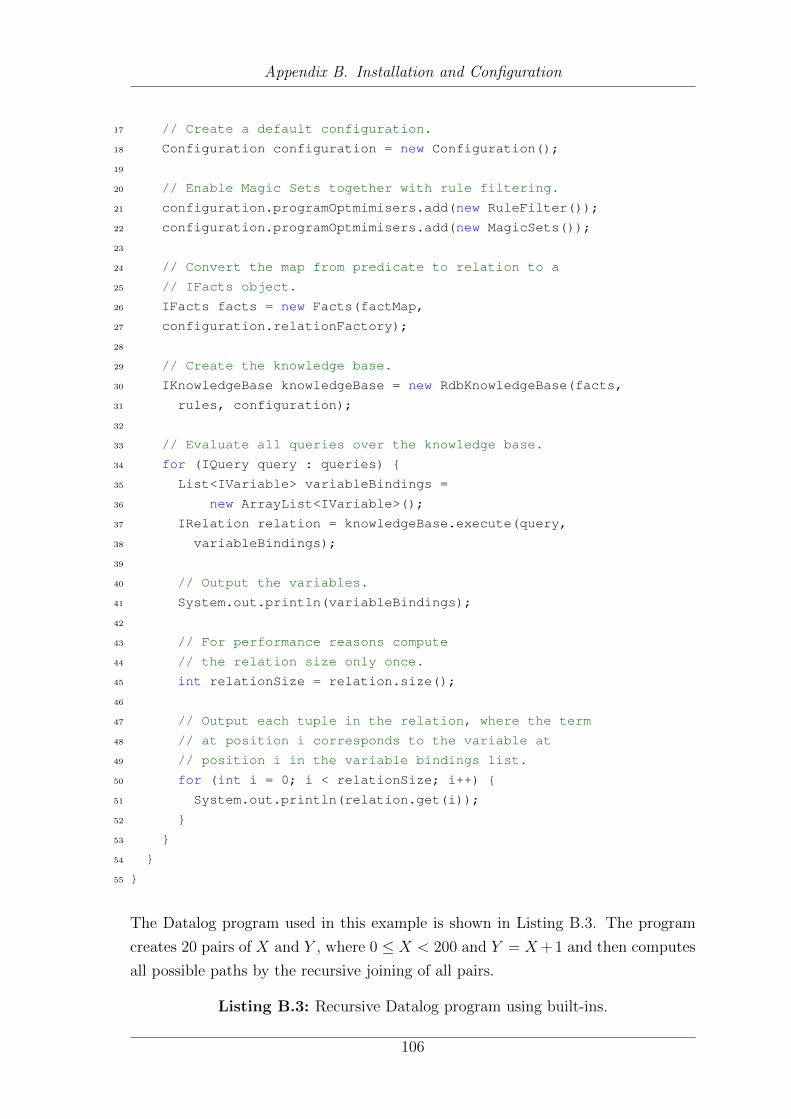
Appendix B. Installation and Configuration
17 // Create a default configuration.
18 Configuration configuration = new Configuration();
19
20 // Enable Magic Sets together with rule filtering.
21 configuration.programOptmimisers.add(new RuleFilter());
22 configuration.programOptmimisers.add(new MagicSets());
23
24 // Convert the map from predicate to relation to a
25 // IFacts object.
26 IFacts facts = new Facts(factMap,
27 configuration.relationFactory);
28
29 // Create the knowledge base.
30 IKnowledgeBase knowledgeBase = new RdbKnowledgeBase(facts,
31 rules, configuration);
32
33 // Evaluate all queries over the knowledge base.
34 for (IQuery query : queries) {
35 List<IVariable> variableBindings =
36 new ArrayList<IVariable>();
37 IRelation relation = knowledgeBase.execute(query,
38 variableBindings);
39
40 // Output the variables.
41 System.out.println(variableBindings);
42
43 // For performance reasons compute
44 // the relation size only once.
45 int relationSize = relation.size();
46
47 // Output each tuple in the relation, where the term
48 // at position i corresponds to the variable at
49 // position i in the variable bindings list.
50 for (int i = 0; i < relationSize; i++) {
51 System.out.println(relation.get(i));
52 }
53 }
54 }
55 }
The Datalog program used in this example is shown in Listing B.3. The program
creates 20 pairs of X and Y , where 0 ≤ X < 200 and Y = X+1 and then computes
all possible paths by the recursive joining of all pairs.
Listing B.3: Recursive Datalog program using built-ins.
106

Appendix B. Installation and Configuration
1 p(0, 1).
2 p(?X1, ?Y1) :- p(?X, ?Y), ?X + 1 = ?X1, ?Y + 1 = ?Y1, ?X < 200.
3
4 path(?X, ?Y) :- p(?X, ?Y).
5 path(?X, ?Y) :- path(?X, ?Z), path(?Z, ?Y).
6
7 ?- path(?X, ?Y).
Listing B.4 shows a part of the output produced by the Java program defined in
Listing B.2, which is the result of the query ?- path(?X, ?Y) that gives all the
possible 20503 transitive paths.
Listing B.4: Part of the output of Java program.
1 [?X, ?Y]
2 (0, 1)
3 (0, 2)
4 (0, 3)
5 (0, 4)
6 (0, 5)
7 (0, 6)
8 (0, 7)
9 (0, 8)
10 (0, 9)
11 (0, 10)
107

List of Tables
3.1. Normalization of RIF-BLD formulas. . . . . . . . . . . . . . . . . . . 60
3.2. Normalization of RIF-BLD rules. . . . . . . . . . . . . . . . . . . . . 61
3.3. Normalization of RIF-BLD document formulas and groups. . . . . . . 61
3.4. Lloyd-Topor transformation of RIF-BLD rules. . . . . . . . . . . . . . 62
3.5. Datalog rule generation for RIF-BLD rules. . . . . . . . . . . . . . . . 63
3.6. Datalog rule generation for RIF-BLD condition formulas. . . . . . . . 64
3.7. Datalog rule generation for RIF-BLD atomic formulas. . . . . . . . . 65
3.8. Datalog rule generation for RIF-BLD frames. . . . . . . . . . . . . . . 66
3.9. RIF-BLD semantics in Datalog. . . . . . . . . . . . . . . . . . . . . . 66
4.1. Comparison of IRIS and IRIS-RDB features. . . . . . . . . . . . . . . 69
4.2. Schema of the universe relation. . . . . . . . . . . . . . . . . . . . . . 77
5.1. Results of positive entailment tests. . . . . . . . . . . . . . . . . . . . 85
5.2. Results of negative entailment tests. . . . . . . . . . . . . . . . . . . . 88
5.3. Times for Join1, no query bindings. . . . . . . . . . . . . . . . . . . . 91
5.4. Times for Join1 with first argument bound. . . . . . . . . . . . . . . . 91
5.5. Times for Join1 with second argument bound. . . . . . . . . . . . . . 91
5.6. Times for Join2. . . . . . . . . . . . . . . . . . . . . . . . . . . . . . . 92
5.7. Times for DBLP. . . . . . . . . . . . . . . . . . . . . . . . . . . . . . 93
5.8. Times for program with built-in predicates. . . . . . . . . . . . . . . . 93
108

List of Listings
2.1. RIF-BLD Annotations. . . . . . . . . . . . . . . . . . . . . . . . . . . 39
5.1. Rules for Join1. . . . . . . . . . . . . . . . . . . . . . . . . . . . . . . 90
5.2. Queries for Join1. . . . . . . . . . . . . . . . . . . . . . . . . . . . . . 90
5.3. Rules for Join2. . . . . . . . . . . . . . . . . . . . . . . . . . . . . . . 92
5.4. Rules for DBLP. . . . . . . . . . . . . . . . . . . . . . . . . . . . . . 92
5.5. Queries for DBLP. . . . . . . . . . . . . . . . . . . . . . . . . . . . . 92
B.1. RIF4J Usage example. . . . . . . . . . . . . . . . . . . . . . . . . . . 102
B.2. IRIS-RDB Usage example. . . . . . . . . . . . . . . . . . . . . . . . . 105
B.3. Recursive Datalog program using built-ins. . . . . . . . . . . . . . . . 106
B.4. Part of the output of Java program. . . . . . . . . . . . . . . . . . . . 107
109

List of Figures
3.1. RIF4J Object Model. . . . . . . . . . . . . . . . . . . . . . . . . . . . 55
3.2. RIF-BLD reasoning architecture. . . . . . . . . . . . . . . . . . . . . 58
4.1. Stratified evaluation strategy. . . . . . . . . . . . . . . . . . . . . . . 71
110

Bibliography
[1] The ISO Common Logic Standard. http://www.common-logic.org,
2007. (last checked March, 2011).
[2] Francois Bancilhon, David Maier, Yehoshua Sagiv, and Jeffrey D Ullman. Magic
sets and Other Strange Ways to Implement Logic Programs (Extended Ab-
stract). In 5th ACM SIGACT-SIGMOD Symposium on Principles of Database
Systems, pages 1–15, 1986.
[3] Jie Bao, Boris Motik, Peter F. Patel-Schneider, and Axel Polleres.
rdf:PlainLiteral: A Datatype for RDF Plain Literals. W3C Recommendation,
http://www.w3.org/TR/rdf-plain-literal/, October 2009.
[4] Chitta Baral and Michael Gelfond. Logic Programming and Knowledge Rep-
resentation. Journal of Logic Programming, 19(20):73–148, 1994.
[5] Mark Birbeck and Shane McCarron. CURIE Syntax 1.0: A syntax for express-
ing Compact URIs. W3C Working Group Note, http://www.w3.org/TR/
2010/NOTE-curie-20101216/, January 2009. (last checked March, 2011).
[6] Paul V. Biron and Ashok Malhotra. XML Schema Part 2: Datatypes
Second Edition. W3C Recommendation, http://www.w3.org/TR/
xmlschema-2/, October 2004.
[7] Harold Boley, Gary Hallmark, Michael Kifer, Adrian Paschke, Axel Polleres,
and Dave Reynolds. RIF Core. W3C Recommendation, http://www.w3.
org/TR/rif-core/, June 2010.
[8] Harold Boley and Michael Kifer. RIF Basic Logic Dialect. W3C Recommen-
111

Bibliography
dation, http://www.w3.org/TR/rif-bld/, June 2010.
[9] Harold Boley and Michael Kifer. RIF Framework for Logic Dialects. W3C
Recommendation, http://www.w3.org/TR/rif-fld/, June 2010.
[10] Stefano A. Ceri, Georg Gottlob, and Letizia Tanca. What You Always Wanted
to Know About Datalog (And Never Dared to Ask). IEEE Transaction on
Knowledge and Data Engineering, 1(1):146–166, March 1989.
[11] Christian de Sainte Marie, Gary Hallmark, and Adrian Paschke. RIF Pro-
duction Rule Dialect. W3C Recommendation, http://www.w3.org/TR/
rif-prd/, June 2010.
[12] Keith L. Clark. Negation as Failure. In Jack Minker, editor, Logic and Data
Bases, volume 1, pages 293–322. Plenum Press, New York, London, 1978.
[13] Jos de Bruijn, Dieter Fensel, Uwe Keller, Michael Kifer, Holger Lausen,
Reto Krummenacher, Axel Polleres, and Livia Predoiu. Web Service Mod-
eling Language (WSML). W3C Member Submission, http://www.w3.org/
Submission/WSML/, June 2005.
[14] Jeffrey Dean and Sanjay Ghemawat. MapReduce: Simplified Data Processing
on Large Clusters. Communications of the ACM, 51(1):107–113, January 2008.
[15] Martin Duerst and Michel Suignard. RFC3987 - Internationalized Resource
Identifiers (IRIs). Request for Comments, IETF RFC3987, http://www.
ietf.org/rfc/rfc3987.txt, January 2005. (last checked March, 2011).
[16] Florian Fischer, Ioan Toma, Valer Roman, Adrian Marte, and Iker Larizgoitia.
D4.4.2 Implementation of Rule-based Reasoning Plug-in. LarKC project deliv-
erable, March 2011.
[17] Sumit Ganguly, Avi Silberschatz, and Shalom Tsur. A Framework for the
Parallel Processing of Datalog Queries. ACM SIGMOD Record, 19(2):143–152,
June 1990.
[18] Michael Gelfond and Vladimir Lifschitz. The Stable Model Semantics For Logic
Programming. In 5th International Conference on Logic Programming, pages
1070–1080. The MIT Press, 1988.
[19] Stephan Grimm, Uwe Keller, Holger Lausen, and Gabor Nagypal. A Reason-
ing Framework for Rule-Based WSML. In 4th European conference on The
112

Bibliography
Semantic Web: Research and Applications, pages 114–128, 2007.
[20] Pascal Hitzler, Markus Krotzsch, Bijan Parsia, Peter F. Patel-Schneider, and
Sebastian Rudolph. OWL 2 Web Ontology Language Primer. W3C Recom-
mendation, http://www.w3.org/TR/owl-primer/, October 2009.
[21] IRIS Reasoner. IRIS - Integrated Rule Inference System - API and User Guide.
http://iris-reasoner.org/pages/user_guide.pdf, 2008.
[22] Jos de Bruijn. RIF RDF and OWL Compatibility. W3C Recommendation,
http://www.w3.org/TR/rif-rdf-owl/, June 2010.
[23] Michael Kifer, Georg Lausen, and James Wu. Logical Foundations of Object-
Oriented and Frame-Based Languages. Journal of the ACM, 42(4):741–843,
1995.
[24] Robert A. Kowalski. Predicate Logic as a Programming Language. In Informa-
tion Processing 74, pages 569–574. IFIP, North-Holland Publishing Company,
1974.
[25] Reto Krummenacher, Daniel Winkler, and Adrian Marte. WSML2Reasoner - A
Comprehensive Reasoning Framework for the Semantic Web. In International
Semantic Web Conference 2010 Posters and Demonstrations Track: Collected
Abstracts, volume 658, pages 125–128, November 2010.
[26] Senlin Liang, Paul Fodor, Hui Wan, and Michael Kifer. OpenRuleBench: An
Analysis of the Performance of Rule Engines. In 18th International Conference
on World Wide Web, pages 601–610, 2009.
[27] Senlin Liang, Paul Fodor, Hui Wan, and Michael Kifer. OpenRuleBench: De-
tailed Report, May 2009.
[28] John W Lloyd and Rodney W. Topor. Making Prolog More Expressive. Journal
of Logic Programming, 1(3):225–240, October 1984.
[29] Ashok Malhotra, Jim Melton, and Norman Walsh. XQuery 1.0 and XPath 2.0
Functions and Operators. W3C Recommendation, http://www.w3.org/
TR/xpath-functions/, January 2007.
[30] Adrian Marte. D3.2.8 Enhanced Reasoning Framework Core. SOA4All project
deliverable, February 2011.
[31] Jack Minker, editor. Foundations of Deductive Databases and Logic Program-
113

Bibliography
ming. Morgan Kaufmann Publishers Inc., San Francisco, CA, USA, 1988.
[32] Stella Mitchell, Leora Morgenstern, and Adrian Paschke. RIF Test Cases. W3C
Working Draft, http://www.w3.org/TR/rif-test/, June 2010.
[33] Axel Polleres, Harold Boley, and Michael Kifer. RIF Datatypes and Built-ins
1.0. W3C Recommendation, http://www.w3.org/TR/rif-dtb/, June
2010.
[34] Konstantinos Sagonas, Terrance Swift, and David S. Warren. XSB as an Ef-
ficient Deductive Database Engine. In In Proceedings of the ACM SIGMOD
International Conference on the Management of Data, pages 442–453. ACM
Press, 1994.
[35] Jeffrey D. Ullman. Principles of Database and Knowledge-Base Systems, Vol-
ume I: Classical Database Systems. Computer Science Press, Inc., New York,
NY, USA, 1988.
[36] Jeffrey D. Ullman. Principles of Database and Knowledge-Base Systems: Vol-
ume II: The New Technologies. W. H. Freeman & Co., New York, NY, USA,
1990.
[37] Maarten H. van Emden and Robert A. Kowalski. The Semantics of Predicate
Logic as a Programming Language. Journal of ACM, 23(4):733–742, October
1976.
[38] Alen van Gelder, Kenneth A. Ross, and John S. Schlipf. The Well-Founded
Semantics for General Logic Programs. Journal of ACM, 38(3):619–649, July
1991.
[39] Daniel Winkler and Barry Bishop. D3.2.5 Second Prototype Repository Rea-
soner for WSML-Core v2.0. SOA4All project deliverable, February 2010.
[40] Daniel Winkler, Reto Krummenacher, and Adrian Marte. RIF-BLD Reasoning
with IRIS. In RuleML-2010 Challenge, October 2010.
[41] Daniel Winkler and Matthias Pressnig. D3.2.6 Second Prototype Rule Reasoner
for WSML-Rule v2.0. SOA4All project deliverable, August 2010.
114