Geometric design

It includes the specific design elements of a highway, such as ◦ the number of lanes, ◦ lane width, ◦ median type and width, ◦ length of freeway acceleration and deceleration

lanes, ◦ need for truck climbing lanes for highways on

steep grades, ◦ and radii required for vehicle turning

Introduction

All these elements and the performance characteristics of vehicles play an important role.

Physical dimensions of vehicles affect a number of design elements such as the ◦ radii required for turning◦ Height of highway overpass◦ Lane width

The alignment of a highway is a three dimensional problem with measurement in x, y and z direction.

It is a bit complicated, therefore the alignment problem is typically reduced to two dimensional alignment as shown in figure on next slide.

Principles of Highway Alignment

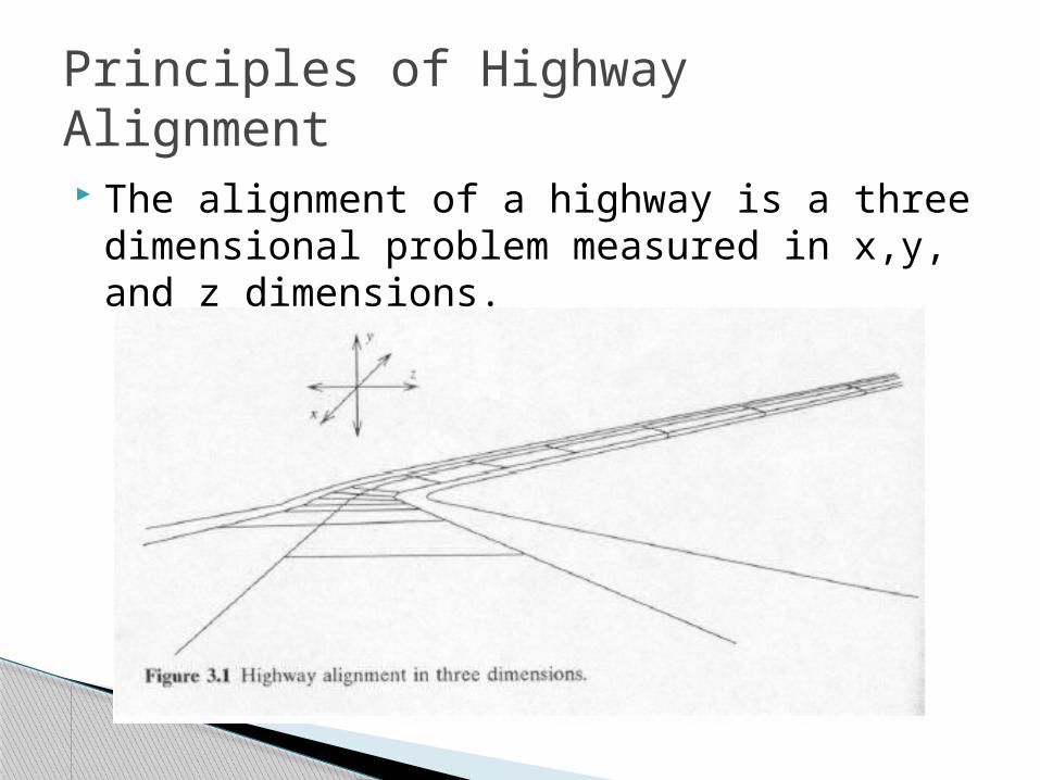
The alignment of a highway is a three dimensional problem measured in x,y, and z dimensions.

Principles of Highway Alignment

Horizontal alignment of road shown in x and z coordinates called the plan view.

Vertical alignment of the road is shown on the y axis and is called the profile view.

Three dimensional problemreduced to two:

Principles of Highway Alignment

Further simplified by using highway position and length instead of x and y.

Distances are measured in terms of stations, with each station consisting of 100ft of highway alignment distance.

For example, a point 4250 ft from a specified origin is said to be at station 42+50

The point of origin is at station 0 + 00

Specifies the elevations of points along a roadway.

Elevations are determined by need to provide proper drainage and driver safety.

A primary concern of vertical alignment is to establish a transition between two roadway grades by means of a vertical curve.

Vertical Alignment

Two types of Vertical Curves:1. Crest Vertical Curves.2. Sag Vertical Curves.

Vertical Alignment

The initial road grade is called G1 the final road grade is called G2 and is typically given in percent.

PVC is the initial point of the vertical curve. The point of intersection of the initial tangent grade

and the final tangent grade is the point of vertical intersection (PVI).

The absolute value of the difference between G1 and G2 is called A and is given in percent.

The point of intersection of the vertical curve with the final tangent grade is called the PVT .

The length (L) of the vertical curve is the horizontal distance between PVC and PVT.

Equal Tangent, if PVC to PVI is L/2.

Vertical Curve Properties

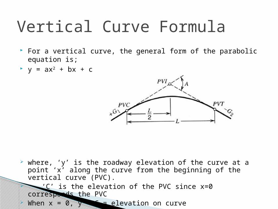
For a vertical curve, the general form of the parabolic equation is; y = ax2 + bx + c

where, ‘y’ is the roadway elevation of the curve at a point ‘x’ along the curve from the beginning of the vertical curve (PVC).

‘C’ is the elevation of the PVC since x=0 corresponds the PVC

When x = 0, y = C = elevation on curve

Vertical Curve Formula

To define ‘a’ and ‘b’, first derivative of equation gives the slope.

At PVC, x=0;

Slope of Curve

baxdx

dy2

bdx

dy

dx

dyG

bG 1

Where G1 is the initial slope.

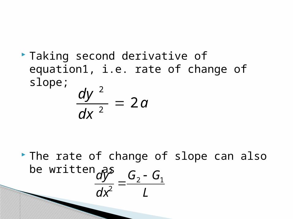
Taking second derivative of equation1, i.e. rate of change of slope;

The rate of change of slope can also be written as

adx

dy2

2

2

L

GG

dx

dy 122

2

Equating equations

or

L

GGa 122

L

GGa

212

Offsets from the initial tangent (profile grade line) are very important in vertical curve design and construction.

Y is defined as the offset at any distance, x, from the PVC.

Properties of Vertical Curves

Y = the offset at any distance, x, from the PVC Ym = the midcurve offset A is theof the difference in the grades. L = the length of the vertical curve x = the distance from the PVC

Other Vertical Curve Relationships

In above equations, 200 is used in the denominator instead of, 2, because A (IG1 – G2I), is expressed in percent rather than ft/ft.

Vertical Alignment

By definition, K (rate of vertical curvature) is the horizontal distance in ft (meters) required to affect a 1% change in the slope of a vertical curve. It has several uses including simplifying the computation of the high/low points of vertical curves. K is calculated as follows.

K= L/A L is in ft (meters) , A is in percent.

The following equation is used to determine the horizontal distance xhl to the high/low point in meters, given that the point does not occur at the PVC or PVT

G1 is the absolute value of the initial grade in percent. In equation G1 was in m/m.

It is the sum of;◦ Vehicle stopping distance &◦ Distance traveled during perception / reaction

time

Stopping Sight Distance

Vehicle stopping distance is calculated by the following formula

where V1 initial speed of vehicle

f frictionG percent grade

Vehicle Stopping Distance

)(2

21

Gfg

vd

It is calculated by the following formuladr = V1* tr

where V1 Initial Velocity of vehicletr time required to perceive

and react to the need to stop

Distance Traveled During Perception/ Reaction Time

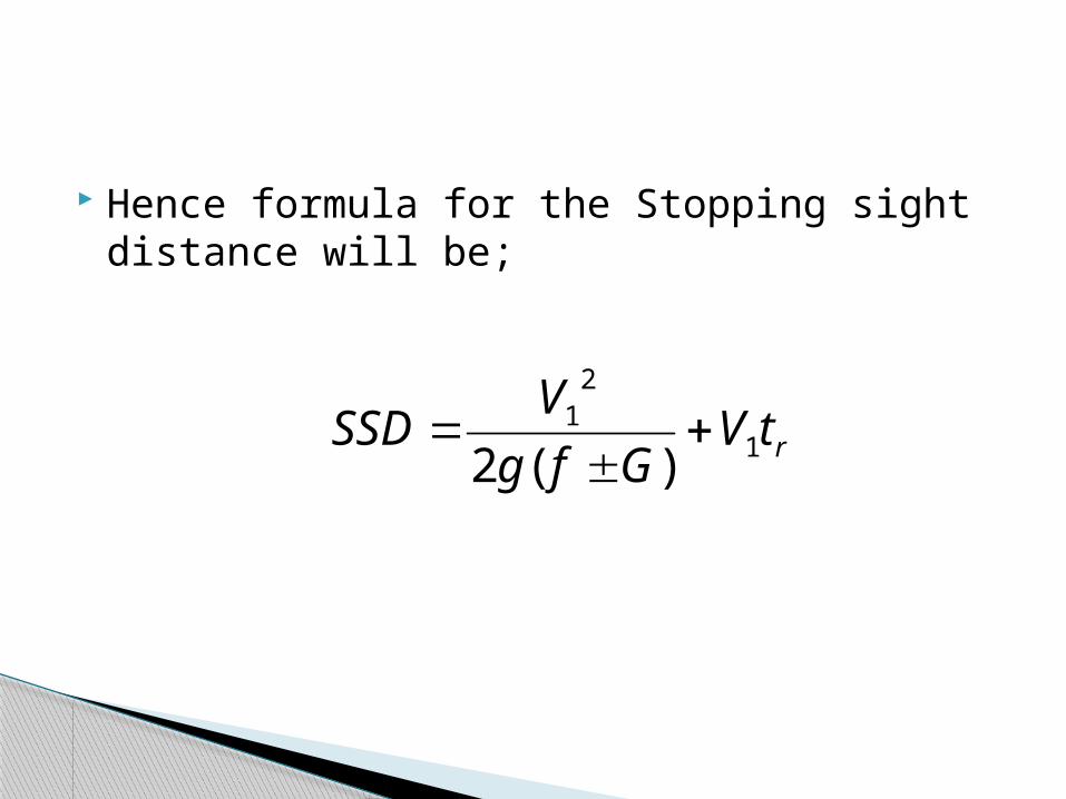
Hence formula for the Stopping sight distance will be;

rtVGfg

VSSD 1

21

)(2

In providing the sufficient SSD on a vertical curve, the length of curve ‘L’ is the critical concern.

Longer lengths of curve provide more SSD, all else being equal, but are most costly to construct.

Shorter curve lengths are relatively inexpensive to construct but may not provide adequate SSD.

SSD and Crest Vertical Curve

In developing such an expression, crest and sag vertical curves are considered separately.

For the crest vertical curve case, consider the diagram.

SSD and Crest Vertical Curve

H1= height of driver’s eye above road-way surface (ft)

H2= height of roadway object (ft)

For a required sight distance S is calculated as follows;

If S>L

S<L

Minimum Length of the Curve

A

HHSLm

221 )(200

2

221

2

)(200 HH

ASLm

For the sight distance required to provide adequate SSD, standard define driver eye height H1 is 3.5 ft and object height H2 is 2 ft. S is assumed is equal to SSD. We get

SSD>L

ASSDLm

21582

SSD<L

2158

2AxSSDLm

Sight distances on crest curves

Working with the above equations can be cumbersome.

To simplify matters on crest curves computations, K- values, are used.

L = K*A

where k is the horizontal distance in feet, required to affect 1 percent change in slope.

Assistant with Target Rod (2ft object height)

Observer with Sighting Rod (3.5 ft)

From Green book

Since you do not at first know L, try one of these equations and compare to requirement, or use L = KA (see tables and graphs in Green Book for a given A and design speed)

Design of vertical curves

Sag vertical curve design differs from crest vertical curve design in the sense that sight distance is governed by night time conditions, because in daylight, sight distance on a sag vertical curve is unrestricted.

The critical concern for sag vertical curve is the headlight sight distance which is a function of the height of the head light above the road way, H, and the inclined upward angle of the head light beam, relative to the horizontal plane of the car, β.

SSD and Sag Vertical Curve

The sag vertical curve sight distance problem is illustrated in the following figure.

By using the properties of parabola for an equal tangent curve, it can be shown that minimum length of the curve, Lm for a required sight distance is

For S>L

For S<L

A

SHSLm

)tan(2002

)tan(200

2

SH

ASLm

For the sight distance required to provide adequate SSD, use a head light height of 2.0 ft and an upward angle of 1 degree.

Substituting these design standards and S = SSD in the above equations;

For SSD>L

For SSD<LA

SSDSSDLm

5.34002

SSD

ASSDLm

5.3400

2

After the location of a road has been determined and the necessary fieldwork has been obtained, the engineer designs or fixes (sets) the grades. A number of factors are considered, including the intended use and importance of the road and the existing topography. If a road is too steep, the comfort and safety of the users and fuel consumption of the vehicles will be adversely affected; therefore, the design criteria will specify maximum grades.  

Design of curves

Typical maximum grades are a 4-percent desired maximum and a 6-percent absolute maximum for a primary road. (The 6 percent means, as indicated before, a 6-foot rise for each 100 feet ahead on the road.) For a secondary road or a major street, the maximum grades might be a 5-percent desired and an 8-percent absolute maximum; and for a tertiary road or a secondary street, an 8-percent desired and a 10-percent (or perhaps a 12-percent) absolute maximum. Conditions may sometimes demand that grades or ramps, driveways, or short access streets go as high as 20 percent. The engineer must also consider minimum grades.

Cont..,

A street with curb and gutter must have enough fall so that the storm water will drain to the inlets; 0.5 percent is a typical minimum grade for curb and gutter (that is, 1/2 foot minimum fall for each 100 feet ahead). For roads with side ditches, the desired minimum grade might be 1 percent; but since ditches may slope at a grade different from the pavement, a road may be designed with a zero-percent grade. Zero-percent grades are not unusual, particularly through plains or tidewater areas.

Cont..,

Another factor considered in designing the finished profile of a road is the earthwork balance; that is, the grades should be set so that all the soil cut off of the hills may be economically hauled to fill in the low areas. In the design of urban streets, the best use of the building sites next to the street will generally be more important than seeking an earthwork balance.

Cont..,

The horizontal distance from the beginning to the end of the curve; the length of the curve is NOT the distance along the parabola itself.

The longer a curve is, the more gradual the transition will be from one grade to the next; the shorter the curve, the more abrupt the change. The change must be gradual enough to provide the required sight distance

Cont..,

The sight distance requirement will depend on the speed for which the road is designed; whether passing or non-passing distance is required; and other assumptions, such as one’s reaction time, braking time, stopping distance, height of one’s eyes, and height of objects. A typical eye level used for designs is 4.5 feet or, more recently, 3.75 feet; typical object heights are 4 inches to 1.5 feet. For a sag curve, the sight distance will usually not be significant during daylight; but the nighttime sight distance must be considered when the reach of headlights may be limited by the abruptness of the curve.

Cont..,