cronus.uwindsor.cacronus.uwindsor.ca/units/isplab/isplab.nsf... · iii declaration “i, hubert...

Neuro-Fuzzy Forecasting of Tourist Arrivals

Doctor of Philosophy Thesis

Hubert Preman Fernando

Volume I

School of Applied Economics Faculty of Business and Law

Victoria University

ii

Abstract

This study develops a model to forecast inbound tourism to Japan, using a

combination of artificial neural networks and fuzzy logic and compares the

performance of this forecasting model with forecasts from other quantitative

forecasting methods namely, the multi-layer perceptron neural network model, the

error correction model, the basic structural model, the autoregressive integrated

moving average model and the naïve model.

Japan was chosen as the country of study mainly due to the availability of reliable

tourism data, and also because it is a popular travel destination for both business and

pleasure. Visitor arrivals from the 10 most popular tourist source countries to Japan,

and total arrivals from all countries were used to incorporate a fairly wide variety of

data patterns in the testing process.

This research has established that neuro-fuzzy models can be used effectively in

tourism forecasting, having made adequate comparisons with other time series and

econometric models using real data. This research takes tourism forecasting a major

leap forward to an entirely new approach in time series pedagogy. As previous

tourism studies have not used hybrid combinations of neural and fuzzy logic in

tourism forecasting this research has only touched the surface of a field that has

immense potential not only in tourism forecasting but also in financial time series

analysis, market research and business analysis.

iii

Declaration

“I, Hubert Preman Fernando, declare that the PhD thesis entitled Neuro-Fuzzy

Forecasting of Tourist Arrivals is no more than 100,000 words in length, exclusive of

tables, figures, appendices, references and footnotes. This thesis contains no material

that has been submitted previously, in whole or in part, for the award of any other

academic degree or diploma. Except where otherwise indicated, this thesis is my own

work”.

Signature: Date: 2 November 2005

iv

Acknowledgements I would like to express my sincere thanks to Professor Lindsay Turner, for his

academic and intellectual guidance, advice, assistance, encouragement and support

during the course of this research study, and the preparation of this thesis. I consider

myself very fortunate to have had Professor Turner as my principal supervisor not

only because of his excellent supervision but also because I was able to draw on his

wide knowledge and expertise in tourism economics and forecasting techniques.

I would also like to thank Dr. Leon Reznik, for introducing me to fuzzy logic, Dr.

Nada Kulendran for his advice on the application of the Error Correction Model and

Miss. Angelina Veysi and Miss Linda Osti for their assistance with data processing.

I would also like to thank my wife Kumarie, and two daughters Nikoli and Sohani for

their understanding, encouragement, support and immense patience during this period,

when they were in fact, deprived of my time and attention.

I dedicate this thesis to my late parents Hubert and Etta and my only sibling the late

Ramyani, who were also deprived of my time and attention during the final months of

their lives.

v

Contents

Page

Abstract ii

Declaration iii

Acknowledgements iv

Volume I

Chapter 1 Introduction 1

1.1 Overview of the Thesis 3

1.2 The Research Problem 4

1.3 Aims and Objectives 8

1.4 Research Methodology 9

1.5 Data Content and Sources 17

1.6 Tourism in Japan 19

1.7 Visitor Arrivals to Japan 22

1.8 Japan's Economy 28

1.9 Japan's International Trade 33

Chapter 2 Literature Review 38

2.1 Introduction 38

2.2 Univariate Time Series Models 41

2.3 Econometric Models 45

2.4 Artificial Neural Networks (ANNs) 49

2.5 Fuzzy Logic 57

2.6 Neuro-Fuzzy Models 61

2.7 Neuro-Fuzzy modeling of Time Series 66

vi

Chapter 3 Neural Network Multi-layer Perceptron Models 67

3.1 Introduction 67

3.2 The Multi-Layer Perceptron Model 68

3.3 The Naïve Model 75

3.4 MLP Non-Periodic Forecasts 76

3.5 MPL Differenced Non-Periodic Forecast 83

3.6 MLP Partial Periodic Forecast 90

3.7 MLP Differenced Partial Periodic Forecast 97

3.8 MLP Periodic Forecast 104

3.9 Naïve Forecasts 111

3.10 Differenced and Undifferenced Model Comparison 118

3.11 MLP Model Comparison with the Naïve 125

3.12 Conclusion 131

Chapter 4 ARIMA and BSM Forecasting 133

4.1 Introduction 133

4.2 The ARIMA Model 134

4.3 The Basic Structural Model 137

4.4 Results of ARIMA(1) Forecasts 139

4.5 Results of ARIMA(1)(12) Forecasts 156

4.6 Results of BSM Forecasts 173

4.7 Model Comparison: ARIMA(1) and ARIMA(1)(12) 184

4.8 Model Comparison: ARIMA, BSM and Naïve Models 189

4.9 Conclusion 196

vii

Chapter 5 ECM and Multivariate Neural Network Forecasting 198


5.2 The Error Correction Model (ECM) 200

5.3 The Multivariate Multi-layer Perceptron (MMLP) Model 204

5.4 Results of ECM Forecasts 207

5.5 Results of Multivariate Multi-layer Perceptron (MMLP) 247

5.6 Model Comparison 254

5.7 Conclusion 260

Volume II

Chapter 6 Adaptive Neuro-Fuzzy Forecasting 261


6.2 The ANFIS Model 262

6.3 The Multivariate ANFIS Model 266

6.4 Results of ANFIS Forecasts 267

6.5 Results of Multivariate ANFIS Forecasts 275

6.6 Univariate and Multivariate ANFIS Model Comparison 282

6.7 Conclusion 289

Chapter 7 Conclusion 291


7.2 Comparison of all models with the Naïve model 294

7.3 Comparison of all models against each other 301

7.4 Summary of conclusions 311

7.5 Recommendations for future research 319

References 321

viii

Appendix I 353

Appendix II 453

List of Figures

Figure 1.1 Total Monthly Arrivals from all Countries to Japan,

1st difference and 1st & 12th difference 18

Figure 1.2 Total Visitor Arrivals to Japan from 1964 to 2004 23

Figure 1.3 Tourist, Business and Other Arrivals to Japan

from 1978 to 2003 24

Figure 1.4 Japan's Economic Growth Rates 29

Figure 1.5 Japan's International Trade from 1978 to 2003 37

Figure 2.1 Basic Structure of an Artificial Neural Network 51

Figure 2.2 MLP Neural Network for Univariate Forecasting 52

Figure 2.3 MLP Neural Network for Multivariate Forecasting 53

Figure 2.4 Membership Functions of a Tourist Arrival System 59

Figure 3.1 Connectionist MLP Model for Univariate Forecasting 69

Figure 5.1 Connectionist MLP Model for Multivariate Forecasting 204

Figure 6.1 Connectionist ANFIS Model 264

Figure 7.1 The total number of forecasts with MAPE lower than

in the naïve model 300

Figure 7.2 The number of paired model comparisons with a significantly

lower MAPE 309

Figure 7.3 The number of forecasts with MAPE less than 10% 310

ix

List of Tables

Table 1.1 Data Structure 12

Table 1.2 Visitor Arrivals to Japan in 2000 by Gender and Age. 25

Table 1.3 Number of International Conventions and Participants 26

Table 1.4 Top 12 Countries of Visitor Origin from 1995 to 2003 27

Table 3.10.1 Univariate one month-ahead Forecasting Performance of

Differenced and Undifferenced Neural Network Models 121

Table 3.10.2 Univariate 12 months-ahead Forecasting Performance of




Table 3.10.4 Forecasting Performance Comparison Summary of



Neural Network and Naïve Forecasts 128








ARIMA(1) and ARIMA(1)(12) Models 186



x






ARIMA and Basic Structural Models 193







Table 5.6.1 Multivariate one month-ahead Forecasting Performance of

ECM and MMLP Models 256

Table 5.6.2 Multivariate 12 months-ahead Forecasting Performance of


Table 5.6.3 Multivariate 24 months-ahead Forecasting Performance of



Multivariate ECM and MMLP Models 259

Table 6.6.1 One month-ahead Forecasting Performance of

ANFIS and MLP Models 286

Table 6.6.2 12 months-ahead Forecasting Performance of ANFIS

and MLP Models 287

xi

Table 6.6.3 24 months-ahead Forecasting Performance of ANFIS

and MLP Models 288


ANFIS and MLP Models 289

Table 7.2.1 One month-ahead Forecasting Performance (MAPE)

comparison for all models against the naïve model 296

Table 7.2.2 12 months-ahead Forecasting Performance (MAPE)


Table 7.2.3 24 months-ahead Forecasting Performance (MAPE)


Table 7.2.4 Forecasting Performance Comparison Summary

for all models against the naïve model 299

Table 7.3.1 Paired comparison of all models, to identify significant

MAPE differences for arrivals from all countries 303


MAPE differences for arrivals from Australia 304


MAPE differences for arrivals from Canada 304


MAPE differences for arrivals from China 305


MAPE differences for arrivals from France 305


MAPE differences for arrivals from Germany 306

xii


MAPE differences for arrivals from Korea 306


MAPE differences for arrivals from Singapore 307


MAPE differences for arrivals from Taiwan 307


MAPE differences for arrivals from UK 308


MAPE differences for arrivals from USA 308

Table 7.3.12 The most suitable forecasting models for tourist arrivals to

Japan from each source country 311

Table 7.4.1 Ranking the models for forecasting tourist arrivals to

Japan 317

Chapter 7 Conclusion

7.1 Introduction

Most studies in tourism forecasting have used time series or econometric methods. While

there have been major improvements and refinements to these methods over the past 20

years, the basic concept used is that of regression. More recently soft computing methods

have been tested for tourism forecasting but these studies have been mainly limited to the

use of artificial neural networks. The purpose of this research was to explore tourism time

series from a totally new perspective and view the variability of stochastic data as being

fuzzy rather than crisp.

From a practical point of view the use of Mamdami type labels to describe levels of

tourism demand as very high, high, medium, low or very low relative to a recent

historical mean. While further subdivisions such as very high 1, 2 or 3, might be more

acceptable to a practitioner, who could plan the availability of hotel rooms or travel

facilities based on forecast levels of tourist demand, rather than a forecast of a specific

number of arrivals. The concern with a traditional forecast is that by aiming to achieve

crisp accuracy the forecaster may be compromising the process of extracting valid

information from the data series. The fuzzy approach accepts the inherent fuzziness of the

data and forecasts tourism demand as an accurate fuzzy level of demand. However, since

time series data are crisp to begin with, and as the requirement is still for crisp forecasts,

the current state of art in fuzzy time series forecasting is to use Sugeno type models


where crisp data are converted into fuzzy membership functions using neural networks,

and defuzzified forecasts in contemporary crisp form are presented for industry use. One

such application is the ANFIS (Adaptive Neuro-Fuzzy Inference System) model

developed by Jang (1993). Since neuro-fuzzy models have never been applied in tourism

forecasting, except by Fernando, Turner and Reznik (1998 and 1999b), this research tests

the viability of fuzzy logic in tourism forecasting, and whether it is an alternative to time

series and econometric tourism forecasting methods.

Japan was chosen as the country of study mainly due to the availability of reliable

tourism data, and also because it is a popular travel destination for both business and

pleasure. Visitor arrivals from the 10 most popular tourist source countries to Japan, and

total arrivals from all countries were used to incorporate a fairly wide variety of data

patterns in the testing process.

Therefore, the aim of this study is to develop a model to forecast inbound tourism to

Japan, using a combination of artificial neural networks and fuzzy logic and to compare

the performance of this forecasting model with forecasts from other quantitative

forecasting models namely, the multi-layer perceptron neural network model, the error

correction model, the basic structural model, the autoregressive integrated moving

average model and the naïve model.

Monthly data from January 1978 to December 2001 is used as within sample data for

model development, and data from January 2002 to December 2003 is used as out of

sample data, for testing the forecasting accuracy of the models. For each data series


forecasts are made for one-month-ahead, 12-months-ahead and 24-months-ahead

horizons, and for one-year and two-year lead periods.

The forecasting accuracy of the models is measured mainly using MAPE and RMSE. In

almost all forecasts in this study the RMSE has been consistent with the MAPE.

Therefore, when comparing alternative forecasting methods, the model that has

demonstrated the lowest MAPE in most forecasts is adjudged the best model. Other

criteria used for measuring forecasting performance are the number of forecasts with less

than 10% MAPE, and the mean MAPE for all forecasts. Though the mean MAPE is

different for each model, t-tests do not always indicate significant differences, because

the variances of the MAPE values are high. These high variances in the MAPE values are

due to the differences in the data structures of the different source countries responding

differently to the parameters of the different forecasting models. Therefore, to test the

significance of the differences in MAPE values, paired sample t-tests are carried-out

separately for each country.

This study uses 11 sets of data and forecasts with each of them for three time horizons

and two lead periods making a total of 22 forecasts for each time horizon and 66 forecasts

in total using each model. The sample size 66 is considered a sufficiently large sample to

compare the forecasting performance of the models on the basis of the number of

forecasts with the lowest MAPE.

Since the SARS epidemic took place in 2003 and caused a sharp one off down turn in

arrivals to Japan, during the latter part of the out of sample test period, error levels are

expected to be high. Two other significant occurrences that affected tourist flows to Japan


were the 2001 September 11th terrorist attack in the United States and the Asian economic

crisis of 1998. This study does not model these events into the forecasting method as it is

difficult to envisage how long their effect would last, but allows the forecasting methods

to track the change. Though forecasting errors are expected to be high, all models

compete against each other on level ground as they all use identical data.

Forecasts from the naïve model are used as the benchmark for determining the adequacy

of the models tested in this research. If a model cannot outperform naïve forecasts in at

least a majority of test runs, then that model would not be considered adequate for

tourism forecasting.

7.2 Comparison of all models with the Naïve model

The forecasting models used in this study are the Autoregressive Integrated Moving

Average model using first differences (ARIMA(1)), the Basic Structural Model (BSM),

the non-periodic Multilayer-Layer Perceptron model (MLP Non-P), the partial periodic

Multilayer-Layer Perceptron model (MLP PP), the periodic Multilayer-Layer Perceptron

model (MLP P), the Error Correction Model (ECM), the Multivariate Multilayer-Layer

Perceptron model (MMLP), the Multivariate Adaptive Neuro-Fuzzy Inference System

(MANFIS) and the univariate Adaptive Neuro-Fuzzy Inference System (ANFIS).

Tables 7.2.1, 7.2.2 and 7.2.3 show for the one-month-ahead, 12-months-ahead and 24-

months-ahead, forecasting horizons respectively, a comparison of the forecasting

performances of all the above models with those of the naïve model. For each model, the

MAPE of the tourist arrival forecast from each source country is compared against the


MAPE of the corresponding naïve model. The best MAPE count (X) reflects the number

of forecasts where the MAPE of a particular model outperforms that of the naïve model.

Therefore, the number of forecasts where the naïve model outperforms that forecasting

model is (22 - X) as 22 forecasts are made using each model for a particular forecasting

time horizon.

Table 7.2.1 shows that for the one-month-ahead forecasting horizon, the ARIMA(1) model

outperforms the naïve model in almost all forecasts (20 out of 22), while the BSM is the

second best with 19 forecasts better than the naïve, and the MLP partial periodic and the

univariate ANFIS are equal third with 18 better forecasts.

The multivariate ANFIS model and the MLP non-periodic model outperform the naïve in

16 and 15 forecasts respectively. Though all models outperform the naïve in more than

50% of forecasts, the multivariate MLP and the ECM are better than the naïve in only 12

and 13 instances respectively.

For the paired t-tests, at a significance level of 5%, models with p-values less than 5% are

considered significant. In the following tables the sign of the t-value is indicated against

the p-value, a negative sign indicating a better forecasting model with a mean MAPE less

than that of the model it is being compared with. Paired sample t-tests show that for the

one month ahead forecasting horizon, the mean difference between the MAPE of each

model and that of the naïve model is significant for the ARIMA(1), BSM, non-periodic

and partial periodic MLP and ECM models. The mean difference is not significant for

the multivariate MLP and the ANFIS models.


Table 7.2.1 One month ahead Forecasting Performance (MAPE) Comparison of all models against the naïve model Country Forecast ARIMA BSM MLP Non- MLP Partial MLP ECM MMLP MANFIS ANFIS Naïve Lead Periodic Periodic Periodic All 1 year 3.0 3.2 5.5 4.9 5.0 18.6 8.2 4.6 9.9 2 year 8.0 8.1 9.8 10.2 9.3 16.7 12.1 10.6 12.3Australia 1 year 4.6 4.8 5.1 3.7 9.3 4.5 6.4 3.6 10.1 2 year 6.3 6.4 6.6 5.4 11.3 5.9 6.5 5.8 8.6Canada 1 year 6.4 7.5 6.8 5.4 9.7 5.6 7.4 6.6 8.6 2 year 8.3 9.8 10.0 9.0 12.3 9.2 9.9 9.6 10.2China 1 year 12.2 11.2 14.6 10.1 14.4 13.2 7.6 6.1 14.2 2 year 27.0 26.3 28.0 28.3 26.8 30.3 26.3 25.8 27.3France 1 year 4.6 4.6 6.1 4.5 10.7 4.8 5.3 3.9 6.3 2 year 8.1 7.9 8.7 8.0 13.6 8.2 9.3 8.4 9.4Germany 1 year 8.8 10.0 7.1 7.6 12.7 10.5 7.9 6.9 7.9 2 year 9.6 11.1 10.2 9.7 12.5 11.3 11.7 9.1 11.2Korea 1 year 6.6 6.1 9.6 11.5 8.6 16.8 8.0 15.1 10.5 2 year 9.3 8.8 12.3 12.7 11.4 16.9 8.7 14.0 12.8Singapore 1 year 14.0 14.4 22.2 16.3 18.4 13.9 23.2 17.3 21.3 2 year 25.1 26.6 30.2 25.9 24.4 25.0 27.7 26.6 27.7Taiwan 1 year 5.8 6.9 10.4 7.2 5.8 7.5 11.4 10.3 14.2 2 year 26.8 28.6 29.3 31.5 20.6 29.1 31.8 32.0 35.4UK 1 year 15.8 18.0 13.5 20.0 23.5 15.0 34.3 39.9 12.7 2 year 12.9 14.0 13.6 17.9 21.5 14.3 24.2 25.9 13.5USA 1 year 4.6 6.0 6.4 5.2 5.8 5.2 7.5 7.2 8.0 2 year 6.1 8.0 9.4 8.6 7.7 8.1 9.3 9.4 10.4Mean 10.6 11.3 12.5 12.0 13.4 13.2 13.9 13.6 13.7 t-test: p-value -0.01 -0.01 -0.01 -0.01 -0.01 -0.28 0.46 -0.46Count of: MAPE <= 10% 15 14 11 12 0 8 9 13 12 7 Best MAPE Count of 22 forecasts (x) 20 19 15 18 0 12 13 16 18 ( 22-x )

Table 7.2.2 shows that for the 12-months-ahead forecasting horizon, the MLP partial

periodic model outperforms the naïve model in most forecasts (18), while the multivariate

MLP is the second best with 17 forecasts better than the naïve. The ARIMA(1), BSM and

the univariate ANFIS are equal third with 16 better forecasts.

The MLP periodic model and the multivariate ANFIS model outperform the naïve in 15

and 13 forecasts respectively. However, the MLP non-periodic model and the ECM are

better than the naïve in only 11 and 7 instances respectively.


Table 7.2.2 12 months ahead Forecasting Performance (MAPE) Comparison of all models against the naïve model

Country Forecast ARIMA BSM MLP Non- MLP Partial MLP ECM MMLP MANFIS ANFIS Naïve Lead Periodic Periodic Periodic All 1 year 7.6 6.8 7.9 6.5 6.9 5.3 8.8 11.0 6.1 9.9 2 year 10.7 10.2 11.2 10.4 10.7 11.2 11.4 12.7 10.8 12.3Australia 1 year 4.2 4.6 5.7 3.0 3.6 23.5 3.7 9.6 3.5 10.1 2 year 5.8 5.9 6.8 4.9 6.8 19.5 5.0 8.0 5.7 8.6Canada 1 year 6.2 6.3 6.8 5.1 7.4 13.6 5.3 7.0 6.5 8.6 2 year 10.3 9.5 9.9 8.8 12.6 16.1 8.5 9.5 9.9 10.2China 1 year 13.8 13.3 11.3 11.7 12.3 14.9 11.9 7.5 7.6 14.2 2 year 28.7 27.9 27.4 26.1 26.8 31.2 28.8 25.8 27.1 27.3France 1 year 4.6 4.2 6.5 4.1 3.3 15.4 3.8 6.0 7.6 6.3 2 year 7.6 7.5 9.5 7.9 9.5 16.8 7.1 9.3 27.1 9.4Germany 1 year 8.3 8.3 7.2 7.3 8.4 16.6 9.1 8.9 3.9 7.9 2 year 9.0 8.8 10.5 9.5 12.1 16.7 10.7 12.0 8.5 11.2Korea 1 year 5.6 5.7 12.7 12.7 9.2 8.0 10.1 14.2 18.1 10.5 2 year 10.1 9.5 15.0 15.4 11.6 11.7 12.5 12.0 16.7 12.8Singapore 1 year 15.7 19.1 21.6 16.7 15.0 20.8 15.6 23.8 17.3 21.3 2 year 26.3 27.5 28.1 25.2 24.2 40.7 27.3 27.2 26.4 27.7Taiwan 1 year 9.1 11.5 12.6 7.5 9.1 5.0 14.3 12.3 10.9 14.2 2 year 34.4 34.8 34.0 31.6 33.6 41.8 34.4 32.7 32.8 35.4UK 1 year 13.1 29.1 16.6 21.0 22.2 49.5 11.8 137.9 247.0 12.7 2 year 11.0 19.6 19.3 20.1 21.5 48.6 12.5 76.1 129.2 13.5USA 1 year 8.8 8.3 7.6 6.1 7.0 6.4 14.7 8.2 7.4 8.0 2 year 12.5 12.5 10.6 9.8 10.7 11.1 16.0 9.6 10.1 10.4Mean 12.0 13.2 13.6 12.3 12.9 20.2 12.9 21.9 29.1 13.7t-test: p-value -0.01 -0.29 -0.36 -0.04 -0.16 0.01 -0.09 0.10 0.10Count of: MAPE <= 10% 11 12 9 12 10 4 8 10 10 7 Best MAPE Count of 22 forecasts (x) 16 16 11 18 15 7 17 13 16 ( 22-x )

Paired sample t-tests show that for the 12-months ahead forecasting horizon, the mean

difference between the MAPE of each model and that of the naïve model is significant

only for the ARIMA(1) and the partial periodic MLP models.

Table 7.2.3 shows that for the 24-months-ahead forecasting horizon, the ARIMA(1) model

outperforms the naïve model in most forecasts (19), while the multivariate MLP is the

second best with 18 forecasts better than the naïve and the BSM is third with 17 better

forecasts.


Table 7.2.3 24 months ahead Forecasting Performance (MAPE) Comparison of all models against the naïve model

Country Forecast ARIMA BSM MLP Non- MLP Partial MLP ECM MMLP MANFIS ANFIS Naïve

Lead Periodic Periodic Periodic All 1 year 7.6 6.8 4.4 7.1 7.0 5.3 6.8 7.6 5.3 9.3 2 year 11.8 11.0 10.2 11.4 10.9 10.3 10.3 12.9 10.8 13.9Australia 1 year 4.2 4.6 5.8 5.6 11.6 23.5 5.5 9.7 8.8 10.8 2 year 6.1 6.1 7.0 7.4 13.4 27.6 7.4 14.4 11.7 13.0Canada 1 year 6.2 6.3 6.2 7.8 6.6 13.6 5.8 6.0 11.7 10.4 2 year 11.6 9.8 11.0 10.0 14.3 17.4 9.0 10.2 14.5 12.4China 1 year 13.8 13.3 17.5 20.7 17.9 14.9 14.0 11.4 11.5 21.00 2 year 29.4 28.9 32.3 32.8 30.4 41.3 29.6 32.3 27.6 32.48France 1 year 4.6 4.2 4.4 8.5 5.3 15.4 5.1 8.9 7.3 11.9 2 year 8.8 7.8 9.1 8.8 8.0 18.9 7.1 9.3 8.5 10.6Germany 1 year 8.3 8.3 9.5 8.1 10.2 16.6 9.5 8.4 8.8 10.3 2 year 8.1 7.9 12.8 8.6 11.8 18.7 9.9 9.7 10.7 11.0Korea 1 year 5.6 5.7 19.3 21.6 15.6 8.0 13.9 7.4 26.4 15.9 2 year 9.4 8.5 23.0 24.1 17.6 11.5 17.4 11.7 27.3 18.3Singapore 1 year 15.7 19.1 13.1 13.9 12.6 20.8 14.8 15.6 9.5 9.1 2 year 25.5 28.4 26.5 25.5 22.0 31.7 25.9 27.0 23.7 25.9Taiwan 1 year 9.1 11.5 7.5 8.7 8.5 5.0 8.8 13.5 8.4 10.5 2 year 31.3 31.1 32.6 35.1 37.1 31.5 31.7 30.5 34.0 34.4UK 1 year 13.1 29.1 40.8 97.4 58.1 49.5 14.0 11.7 29.9 79.5 2 year 10.9 36.3 32.0 81.6 45.2 63.6 13.4 93.8 143.2 43.3USA 1 year 8.8 8.3 3.8 4.1 4.3 6.4 9.4 3.2 3.0 2.9 2 year 11.4 10.9 9.3 9.8 10.2 10.7 10.6 10.0 10.4 9.9Mean 11.9 13.8 15.4 20.8 17.2 21.0 12.7 16.6 20.6 18.9t-test: p-value -0.02 -0.02 -0.03 0.18 -0.06 0.18 -0.03 -0.28 0.38Count of: MAPE <= 10% 12 12 10 11 6 4 11 9 8 4 Best MAPE Count of 22 forecasts (x) 19 17 16 14 13 8 18 15 14 ( 22-x )

The MLP non-periodic model and the multivariate ANFIS model outperform the naïve in

16 and 15 forecasts respectively. However, the MLP partial periodic model, the MLP

periodic model and the ECM are better than the naïve in only 14, 14 and 8 instances

respectively.


Paired sample t-tests show that for the 24-months ahead forecasting horizon, the mean

difference between the MAPE of each model and that of the naïve model is significant for

the ARIMA(1), BSM, non-periodic MLP and the multivariate MLP models.

Table 7.2.4 Forecasting Performance Comparison Summary of all models against the naïve model ARIMA BSM MLP Non- MLP Partial MLP ECM MMLP MANFIS ANFIS Naïve Periodic PeriodicPeriodic Mean MAPE 11.5 12.8 13.8 15.1 15.1 18.2 12.9 17.4 21.1 15.5Standard Deviation 7.4 8.8 9.0 15.6 11.3 12.5 7.5 21.1 36.4 11.5t-test: p-value -0.01 -0.01 -0.01 -0.29 -0.03 0.01 -0.02 0.22 0.18Count of : MAPE <= 10% 38 38 30 35 16 16 28 32 30 18 Best MAPE Count of 66 forecasts (x) 55 52 42 50 28 27 48 44 48 (66-x )

Table 7.2.4 shows that in summary, for all three forecasting horizons, the ARIMA1

model outperforms the naïve model in most forecasts (55 out of the total 66), while the

BSM is the second best with 52 of 66 forecasts better than the naïve. The MLP partial

periodic is third with 50 better forecasts.

The univariate ANFIS model and the multivariate MLP model outperform the naïve in 48

out of 66 forecasts each. The multivariate ANFIS mode and the MLP non-periodic model

are better than the naïve in 44 and 42 instances respectively. However, the MLP periodic

and the ECM are better than the naïve model in only 28 and 27 forecasts (which is less

than half the total number of 66 forecasts made) and because of this they are not

considered adequate for forecasting tourist arrivals to Japan. This is despite the p-value of

the periodic MLP model indicating a significantly better mean difference in MAPE

values compared with the naïve model. These findings are shown graphically in Figure

7.1.


Paired sample t-tests show that for all three forecasting horizons, the mean difference

between the MAPE of each model and that of the naïve model is significant for the

ARIMA(1), BSM, non-periodic MLP, periodic MLP and multivariate MLP models.

Figure 7.1 The total number of forecasts with

MAPE lower than in the naïve model

0 10 20 30 40 50 60

ARIMA1

BSM

MLP Partial Periodic

ANFIS

MMLP

MANFIS

MLP Non-Periodic

MLP Periodic

ECM

Fore

cast

ing

Mod

el

Number of Forecasts

Most of the other models do not show a significantly lower MAPE from that of the naïve

even though they out-perform the naïve with lower MAPE values in a large number of

forecasts. This is due to the high variances of the MAPE values, which are in turn due to

differences in the arrival data structures of different countries. For example the MAPE

values for USA are consistently low for all models while those for the UK are high for all

models. This high MAPE variance causes t values to be low despite the MAPE in most

forecasts being less than that of the naïve model.


The relatively poor performance of the regression model is supportive of previous

findings by Martin and Witt (1989a) that the naïve model is significantly accurate relative

to the regression methods. The findings are also supportive of Turner and Witt (2001b) in

that the results tend to confirm the superiority of the ARIMA and BSM time series

models over both regression and the naïve models. The neural network with and without

fuzzy logic outperforms regression and the naïve model but falls short of the ARIMA and

BSM time series methods. The in between position of the neural approach requires

further investigation.

There is no significant difference from the naïve comparison over all time horizons to the

individual findings over each time frame. The sophisticated time series methods, ARIMA

and BSM, are the more accurate forecasting models in all horizons, the regression model

the least accurate and the neural models fall in between or in the shorter time horizons

perform alongside the sophisticated time series models.

7.3 Comparison of all models against each other

Section 7.2 shows the extent to which the models out perform the naïve method. The

model comparisons in section 7.2 were based on the number of forecasts where the

MAPE value of a model was less than that of the naïve model. When comparing all

models against each other, though some models had many forecasts with lower MAPE

values than others, the corresponding mean MAPE of these models were not always

significantly lower. This section shows, using paired sample t-tests, the number of

forecasts in which each model significantly out performs each of the other models and


identifies the better models. Paired sample significance tests are made for each country

based on 6 forecasts using identical arrivals data in all six forecasts. As each model is

compared with 9 other models, for the 11 arrival data sets, 99 paired comparisons are

made for each model. As there are 10 models, 90 paired comparisons are made for each

country. For the paired t-tests, at a significance level of 5%, models with p-values less

than 5% are considered significant. In the following tables the sign of the t-value is

indicated against the p-value, a negative sign indicating a better forecasting model, with a

mean MAPE less than that of the model it is being compared with.

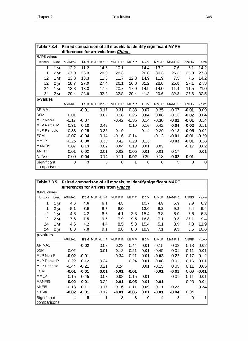
Tables 7.3.1 to 7.3.11 show the MAPE of 6 forecasts from each of the 10 models and p-

values of a paired sample t-test of all 90 pairs of models for arrivals from all countries to

Japan and each of the 10 source countries, respectively. The 6 forecasts represented in

each of the 11 tables are the forecasts for each arrival data source for each of the two lead

periods and each of the three time horizons. Each table represents the analysis of 6 MAPE

values from one arrival data set against those from 9 other models. This method of

analysis using data from one country at a time is undertaken because the magnitude of the

MAPE values associated with certain countries of origin, differ widely from those for

some other countries making statistical analysis difficult due to high MAPE variances.

In Tables 7.3.1 to 7.3.11 each model represented by a column is compared against the

models represented by the rows. The p-values indicate whether the difference in the

MAPE values of the two models is significant. A negative sign assigned to the p-value

indicates a negative t-value and therefore that the former model (represented in a column)

has a lower mean MAPE than the latter (models represented in rows). The last row of the

table shows the number of paired model comparisons where the mean difference in


MAPE values was significant for the model represented in each column. The total

number of these significant mean differences in MAPE for each forecasting model is

presented graphically in Figure 7.2.

Table 7.3.1 Paired comparison of all models, to identify significant MAPE differences for arrivals from all countries

MAPE values Horizon Lead ARIMA1 BSM MLP Non-P MLP P P MLP P ECM MMLP MANFIS ANFIS Naive

1 1 yr 3.0 3.2 5.5 4.9 5.0 18.6 8.2 4.6 9.91 2 yr 8.0 8.1 9.8 10.2 9.3 16.7 12.1 10.6 12.3

12 1 yr 7.6 6.8 7.9 6.5 6.9 5.3 8.8 11.0 6.1 9.912 2 yr 10.7 10.2 11.2 10.4 10.7 11.2 11.4 12.7 10.8 12.324 1 yr 7.6 6.8 4.4 7.1 7.0 5.3 6.8 7.6 5.3 9.324 2 yr 11.8 11.0 10.2 11.4 10.9 10.3 10.3 12.9 10.8 13.9

p-values ARIMA1 BSM MLP Non-P MLP P P MLP P ECM MMLP MANFIS ANFIS Naive

ARIMA1 -0.04 0.47 0.30 -0.04 -0.33 0.10 0.01 0.47 0.01BSM 0.04 0.26 0.06 0.06 0.46 0.07 0.01 0.29 0.01MLP Non-P -0.47 -0.26 0.35 0.31 -0.20 0.06 0.01 -0.39 0.01MLP Partial P -0.30 -0.06 -0.35 0.45 -0.08 0.08 0.01 -0.15 0.01MLP Periodic 0.04 -0.06 -0.31 -0.45 -0.10 0.25 0.03 -0.11 0.01ECM 0.33 -0.46 0.20 0.08 0.10 0.05 0.01 0.17 0.01MMLP -0.10 -0.07 -0.06 -0.08 -0.25 -0.05 -0.27 -0.06 -0.34MANFIS -0.01 -0.01 -0.01 -0.01 -0.03 -0.01 0.27 -0.01 0.16ANFIS 0.47 -0.29 0.39 0.15 0.11 -0.17 0.06 0.01 0.01Naïve -0.01 -0.01 -0.01 -0.01 -0.01 -0.01 0.34 -0.16 -0.01 Significant comparisons

2 3 2 2 3 3 0 0 2 0


Table 7.3.2 Paired comparison of all models, to identify significant MAPE differences for arrivals from Australia


1 1 yr 4.6 4.8 5.1 3.7 9.3 4.5 6.4 3.6 10.11 2 yr 6.3 6.4 6.6 5.4 11.3 5.9 6.5 5.8 8.6

12 1 yr 4.2 4.6 5.7 3.0 3.6 23.5 3.7 9.6 3.5 10.112 2 yr 5.8 5.9 6.8 4.9 6.8 19.5 5.0 8.0 5.7 8.624 1 yr 4.2 4.6 5.8 5.6 11.6 23.5 5.5 9.7 8.8 10.824 2 yr 6.1 6.1 7.0 7.4 13.4 27.6 7.4 14.4 11.7 13.0


ARIMA1 0.02 0.01 -0.34 0.08 0.01 0.35 0.01 0.17 0.01BSM -0.02 0.01 -0.23 0.09 0.01 -0.47 0.01 0.20 0.01MLP Non-P -0.01 -0.01 -0.03 0.16 0.01 -0.04 0.02 0.39 0.01MLP Partial P 0.34 0.23 0.03 0.04 0.01 0.03 0.01 0.05 0.01MLP Periodic -0.08 -0.09 -0.16 -0.04 0.01 -0.06 0.20 -0.04 0.18ECM -0.01 -0.01 -0.01 -0.01 -0.01 -0.01 -0.01 -0.01 -0.01MMLP -0.35 0.47 0.04 -0.03 0.06 0.01 0.01 0.12 0.01MANFIS -0.01 -0.01 -0.02 -0.01 -0.20 0.01 -0.01 -0.01 0.09ANFIS -0.17 -0.20 -0.39 -0.05 0.04 0.01 -0.12 0.01 0.01Naïve -0.01 -0.01 -0.01 -0.01 -0.18 0.01 -0.01 -0.09 -0.01 Significant comparisons

5 4 3 7 1 0 4 1 4 1

Table 7.3.3 Paired comparison of all models, to identify significant MAPE

differences for arrivals from Canada MAPE values Horizon Lead ARIMA1 BSM MLP Non-P MLP P P MLP P ECM MMLP MANFIS ANFIS Naive

1 1 yr 6.4 7.5 6.8 5.4 9.7 5.6 7.4 6.6 8.61 2 yr 8.3 9.8 10.0 9.0 12.3 9.2 9.9 9.6 10.2

12 1 yr 6.2 6.3 6.8 5.1 7.4 13.6 5.3 7.0 6.5 8.612 2 yr 10.3 9.5 9.9 8.8 12.6 16.1 8.5 9.5 9.9 10.224 1 yr 6.2 6.3 6.2 7.8 6.6 13.6 5.8 6.0 11.7 10.424 2 yr 11.6 9.8 11.0 10.0 14.3 17.4 9.0 10.2 14.5 12.4


ARIMA1 0.48 0.22 -0.20 0.03 0.01 -0.05 0.37 0.06 0.01BSM -0.48 0.18 -0.18 0.05 0.01 -0.01 0.19 0.10 0.01MLP Non-P -0.22 -0.18 -0.08 0.05 0.01 -0.01 -0.29 0.12 0.02MLP Partial P 0.20 0.18 0.08 0.08 0.01 -0.14 0.15 0.01 0.01MLP Periodic -0.03 -0.05 -0.05 -0.08 0.01 -0.03 -0.05 0.41 0.46ECM -0.01 -0.01 -0.01 -0.01 -0.01 -0.01 -0.01 -0.01 -0.01MMLP 0.05 0.01 0.01 0.14 0.03 0.01 0.01 0.02 0.01MANFIS -0.37 -0.19 0.29 -0.15 0.05 0.01 -0.01 0.13 0.02ANFIS -0.06 -0.10 -0.12 -0.01 -0.41 0.01 -0.02 -0.13 0.36Naïve -0.01 -0.01 -0.02 -0.01 -0.46 0.01 -0.01 -0.02 -0.36 Significant comparisons

3 3 3 3 1 0 8 3 1 1


Table 7.3.4 Paired comparison of all models, to identify significant MAPE differences for arrivals from China


1 1 yr 12.2 11.2 14.6 10.1 14.4 13.2 7.6 6.1 14.21 2 yr 27.0 26.3 28.0 28.3 26.8 30.3 26.3 25.8 27.3

12 1 yr 13.8 13.3 11.3 11.7 12.3 14.9 11.9 7.5 7.6 14.212 2 yr 28.7 27.9 27.4 26.1 26.8 31.2 28.8 25.8 27.1 27.324 1 yr 13.8 13.3 17.5 20.7 17.9 14.9 14.0 11.4 11.5 21.024 2 yr 29.4 28.9 32.3 32.8 30.4 41.3 29.6 32.3 27.6 32.5


ARIMA1 -0.01 0.17 0.31 0.38 0.07 0.25 -0.07 -0.01 0.09BSM 0.01 0.07 0.18 0.25 0.04 0.08 -0.13 -0.02 0.04MLP Non-P -0.17 -0.07 -0.42 -0.35 0.14 -0.30 -0.02 -0.01 0.14MLP Partial P -0.31 -0.18 0.42 -0.19 0.16 -0.42 -0.04 -0.02 0.11MLP Periodic -0.38 -0.25 0.35 0.19 0.14 -0.29 -0.13 -0.05 0.02ECM -0.07 -0.04 -0.14 -0.16 -0.14 -0.13 -0.01 -0.01 -0.29MMLP -0.25 -0.08 0.30 0.42 0.29 0.13 -0.03 -0.01 0.18MANFIS 0.07 0.13 0.02 0.04 0.13 0.01 0.03 -0.17 0.02ANFIS 0.01 0.02 0.01 0.02 0.05 0.01 0.01 0.17 0.01Naïve -0.09 -0.04 -0.14 -0.11 -0.02 0.29 -0.18 -0.02 -0.01 Significant comparisons

0 3 0 0 1 0 0 5 8 0


differences for arrivals from France MAPE values Horizon Lead ARIMA1 BSM MLP Non-P MLP P P MLP P ECM MMLP MANFIS ANFIS Naive

1 1 yr 4.6 4.6 6.1 4.5 10.7 4.8 5.3 3.9 6.31 2 yr 8.1 7.9 8.7 8.0 13.6 8.2 9.3 8.4 9.4

12 1 yr 4.6 4.2 6.5 4.1 3.3 15.4 3.8 6.0 7.6 6.312 2 yr 7.6 7.5 9.5 7.9 9.5 16.8 7.1 9.3 27.1 9.424 1 yr 4.6 4.2 4.4 8.5 5.3 15.4 5.1 8.9 7.3 11.924 2 yr 8.8 7.8 9.1 8.8 8.0 18.9 7.1 9.3 8.5 10.6


ARIMA1 -0.02 0.02 0.22 0.44 0.01 -0.15 0.02 0.13 0.02BSM 0.02 0.01 0.12 0.21 0.01 -0.45 0.01 0.11 0.01MLP Non-P -0.02 -0.01 -0.34 -0.21 0.01 -0.03 0.22 0.17 0.12MLP Partial P -0.22 -0.12 0.34 -0.24 0.01 -0.08 0.01 0.16 0.01MLP Periodic -0.44 -0.21 0.21 0.24 0.01 -0.15 0.05 0.11 0.05ECM -0.01 -0.01 -0.01 -0.01 -0.01 -0.01 -0.01 -0.09 -0.01MMLP 0.15 0.45 0.03 0.08 0.15 0.01 0.01 0.11 0.01MANFIS -0.02 -0.01 -0.22 -0.01 -0.05 0.01 -0.01 0.23 0.04ANFIS -0.13 -0.11 -0.17 -0.16 -0.11 0.09 -0.11 -0.23 -0.34Naïve -0.02 -0.01 -0.12 -0.01 -0.05 0.01 -0.01 -0.04 0.34 Significant comparisons

4 5 1 3 3 0 4 2 0 1


Table 7.3.6 Paired comparison of all models, to identify significant MAPE differences for arrivals from Germany


1 1 yr 8.8 10.0 7.1 7.6 12.7 10.5 7.9 6.9 7.91 2 yr 9.6 11.1 10.2 9.7 12.5 11.3 11.7 9.1 11.2

12 1 yr 8.3 8.3 7.2 7.3 8.4 16.6 9.1 8.9 3.9 7.912 2 yr 9.0 8.8 10.5 9.5 12.1 16.7 10.7 12.0 8.5 11.224 1 yr 8.3 8.3 9.5 8.1 10.2 16.6 9.5 8.4 8.8 10.324 2 yr 8.1 7.9 12.8 8.6 11.8 18.7 9.9 9.7 10.7 11.0


ARIMA1 0.13 0.20 -0.28 0.04 0.01 0.01 0.05 -0.26 0.05BSM -0.13 0.34 -0.14 0.04 0.01 0.01 0.18 -0.18 0.17MLP Non-P -0.20 -0.34 -0.09 0.18 0.01 0.25 0.39 -0.01 0.22MLP Partial P 0.28 0.14 0.09 0.01 0.01 0.01 0.01 -0.28 0.01MLP Periodic -0.04 -0.04 -0.18 -0.01 0.01 -0.13 -0.13 -0.03 -0.05ECM -0.01 -0.01 -0.01 -0.01 -0.01 -0.01 -0.01 -0.01 -0.01MMLP -0.01 -0.01 -0.25 -0.01 0.13 0.01 -0.24 -0.03 -0.33MANFIS -0.05 -0.18 -0.39 -0.01 0.13 0.01 0.24 -0.06 0.40ANFIS 0.26 0.18 0.01 0.28 0.03 0.01 0.03 0.06 0.01Naïve -0.05 -0.17 -0.22 -0.01 0.05 0.01 0.33 -0.40 -0.01 Significant comparisons

5 3 1 5 1 0 1 1 5 1


differences for arrivals from Korea MAPE values Horizon Lead ARIMA1 BSM MLP Non-P MLP P P MLP P ECM MMLP MANFIS ANFIS Naive

1 1 yr 6.6 6.1 9.6 11.5 8.6 16.8 8.0 15.1 10.51 2 yr 9.3 8.8 12.3 12.7 11.4 16.9 8.7 14.0 12.8

12 1 yr 5.6 5.7 12.7 12.7 9.2 8.0 10.1 14.2 18.1 10.512 2 yr 10.1 9.5 15.0 15.4 11.6 11.7 12.5 12.0 16.7 12.824 1 yr 5.6 5.7 19.3 21.6 15.6 8.0 13.9 7.4 26.4 15.924 2 yr 9.4 8.5 23.0 24.1 17.6 11.5 17.4 11.7 27.3 18.3


ARIMA1 -0.03 0.01 0.01 0.03 0.01 0.05 0.05 0.01 0.01BSM 0.03 0.01 0.01 0.03 0.01 0.01 0.03 0.01 0.01MLP Non-P -0.01 -0.01 0.02 -0.01 -0.02 -0.37 -0.04 0.01 -0.04MLP Partial P -0.01 -0.01 -0.02 -0.01 -0.01 -0.23 -0.03 0.01 -0.01MLP Periodic -0.03 -0.03 0.01 0.01 -0.07 -0.49 -0.26 0.01 0.01ECM -0.01 -0.01 0.02 0.01 0.07 0.01 0.35 0.01 0.02MMLP -0.05 -0.01 0.37 0.23 0.49 -0.01 -0.05 0.05 -0.22MANFIS -0.05 -0.03 0.04 0.03 0.26 -0.35 0.05 0.08 0.07ANFIS -0.01 -0.01 -0.01 -0.01 -0.01 -0.01 -0.05 -0.08 -0.01Naïve -0.01 -0.01 0.04 0.01 -0.01 -0.02 0.22 -0.07 0.01 Significant comparisons

8 9 2 1 4 5 1 3 0 3


Table 7.3.8 Paired comparison of all models, to identify significant MAPE differences for arrivals from Singapore


1 1 yr 14.0 14.4 22.2 16.3 18.4 13.9 23.2 17.3 21.31 2 yr 25.1 26.6 30.2 25.9 24.4 25.0 27.7 26.6 27.7

12 1 yr 15.7 19.1 21.6 16.7 15.0 20.8 15.6 23.8 17.3 21.312 2 yr 26.3 27.5 28.1 25.2 24.2 40.7 27.3 27.2 26.4 27.724 1 yr 15.7 19.1 13.1 13.9 12.6 20.8 14.8 15.6 9.5 9.124 2 yr 25.5 28.4 26.5 25.5 22.0 31.7 25.9 27.0 23.7 25.9


ARIMA1 0.01 0.05 0.37 -0.02 0.02 0.45 0.03 -0.42 0.21BSM -0.01 0.30 -0.05 -0.01 0.07 -0.01 0.21 -0.12 -0.44MLP Non-P -0.05 -0.30 -0.02 -0.03 0.21 -0.05 0.28 -0.01 -0.03MLP Partial P -0.37 0.05 0.02 -0.02 0.03 -0.40 0.01 -0.31 0.17MLP Periodic 0.02 0.01 0.03 0.02 0.01 0.02 0.02 0.29 0.16ECM -0.02 -0.07 -0.21 -0.03 -0.01 -0.01 -0.26 -0.03 -0.12MMLP -0.45 0.01 0.05 0.40 -0.02 0.01 0.04 -0.41 0.20MANFIS -0.03 -0.21 -0.28 -0.01 -0.02 0.26 -0.04 -0.01 -0.06ANFIS 0.42 0.12 0.01 0.31 -0.29 0.03 0.41 0.01 0.02Naïve -0.21 0.44 0.03 -0.17 -0.16 0.12 -0.20 0.06 -0.02 0.00Significant comparisons

4 0 0 4 7 0 4 0 4 1


differences for arrivals from Taiwan MAPE values Horizon Lead ARIMA1 BSM MLP Non-P MLP P P MLP P ECM MMLP MANFIS ANFIS Naive

1 1 yr 5.8 6.9 10.4 7.2 5.8 7.5 11.4 10.3 14.21 2 yr 26.8 28.6 29.3 31.5 20.6 29.1 31.8 32.0 35.4

12 1 yr 9.1 11.5 12.6 7.5 9.1 5.0 14.3 12.3 10.9 14.212 2 yr 34.4 34.8 34.0 31.6 33.6 41.8 34.4 32.7 32.8 35.424 1 yr 9.1 11.5 7.5 8.7 8.5 5.0 8.8 13.5 8.4 10.524 2 yr 31.3 31.1 32.6 35.1 37.1 31.5 31.7 30.5 34.0 34.4


ARIMA1 0.02 0.07 0.26 0.26 -0.30 0.06 0.05 0.07 0.01BSM -0.02 0.37 -0.38 -0.47 -0.17 0.37 0.12 0.30 0.03MLP Non-P -0.07 -0.37 -0.28 0.42 -0.15 -0.44 0.23 0.33 0.01MLP Partial P -0.26 0.38 0.28 0.04 -0.26 0.33 0.15 0.10 0.01MLP Periodic -0.26 0.47 -0.42 -0.04 -0.36 0.46 0.47 -0.30 0.20ECM 0.30 0.17 0.15 0.26 0.36 0.17 0.14 0.16 0.05MMLP -0.06 -0.37 0.44 -0.33 -0.46 -0.17 0.22 0.36 0.02MANFIS -0.05 -0.12 -0.23 -0.15 -0.47 -0.14 -0.22 -0.30 0.06ANFIS -0.07 -0.30 -0.33 -0.10 0.30 -0.16 -0.36 0.30 0.01Naïve -0.01 -0.03 -0.01 -0.01 -0.20 -0.05 -0.02 -0.06 -0.01 Significant comparisons

3 1 1 2 0 1 1 0 1 0


Table 7.3.10 Paired comparison of all models, to identify significant MAPE differences for arrivals from UK


1 1 yr 15.8 18.0 13.5 20.0 23.5 15.0 34.3 39.9 12.71 2 yr 12.9 14.0 13.6 17.9 21.5 14.3 24.2 25.9 13.5

12 1 yr 13.1 29.1 16.6 21.0 22.2 49.5 11.8 137.9 247.0 12.712 2 yr 11.0 19.6 19.3 20.1 21.5 48.6 12.5 76.1 129.2 13.524 1 yr 13.1 29.1 40.8 97.4 58.1 49.5 14.0 11.7 29.9 79.524 2 yr 10.9 36.3 32.0 81.6 45.2 63.6 13.4 93.8 143.2 43.3


ARIMA1 0.01 0.05 0.05 0.03 0.01 0.14 0.03 0.03 0.10BSM -0.01 -0.31 0.10 0.18 0.01 -0.02 0.04 0.04 0.32MLP Non-P -0.05 0.31 0.05 0.04 0.01 -0.05 0.05 0.04 0.19MLP Partial P -0.05 -0.10 -0.05 -0.10 -0.49 -0.05 0.25 0.10 -0.02MLP Periodic -0.03 -0.18 -0.04 0.10 0.07 -0.03 0.14 0.07 0.47ECM -0.01 -0.01 -0.01 0.49 -0.07 -0.01 0.14 0.06 -0.11MMLP -0.14 0.02 0.05 0.05 0.03 0.01 0.03 0.03 0.11MANFIS -0.03 -0.04 -0.05 -0.25 -0.14 -0.14 -0.03 0.03 -0.13ANFIS -0.03 -0.04 -0.04 -0.10 -0.07 -0.06 -0.03 -0.03 -0.06Naïve -0.10 -0.32 -0.19 0.02 -0.47 0.11 -0.11 0.13 0.06 Significant comparisons

7 3 5 0 0 0 7 1 0 1


differences for arrivals from USA MAPE values Horizon Lead ARIMA1 BSM MLP Non-P MLP P P MLP P ECM MMLP MANFIS ANFIS Naïve

1 1 yr 4.6 6.0 6.4 5.2 5.8 5.2 7.5 7.2 8.01 2 yr 6.1 8.0 9.4 8.6 7.7 8.1 9.3 9.4 10.4

12 1 yr 8.8 8.3 7.6 6.1 7.0 6.4 14.7 8.2 7.4 8.012 2 yr 12.5 12.5 10.6 9.8 10.7 11.1 16.0 9.6 10.1 10.424 1 yr 8.8 8.3 3.8 4.1 4.3 6.4 9.4 3.2 3.0 2.924 2 yr 11.4 10.9 9.3 9.8 10.2 10.7 10.6 10.0 10.4 9.9


ARIMA1 0.27 -0.26 -0.12 -0.03 -0.19 0.05 -0.31 -0.29 -0.39BSM -0.27 -0.12 -0.03 -0.04 -0.02 0.10 -0.19 -0.17 -0.28MLP Non-P 0.26 0.12 -0.08 0.22 0.40 0.06 0.36 0.41 0.15MLP Partial P 0.12 0.03 0.08 0.03 0.07 0.04 0.12 0.10 0.08MLP Periodic 0.03 0.04 -0.22 -0.03 0.19 0.03 -0.29 -0.22 -0.29ECM 0.19 0.02 -0.40 -0.07 -0.19 0.06 -0.47 -0.49 -0.41MMLP -0.05 -0.10 -0.06 -0.04 -0.03 -0.06 -0.08 -0.09 -0.11MANFIS 0.31 0.19 -0.36 -0.12 0.29 0.47 0.08 -0.40 0.14ANFIS 0.29 0.17 -0.41 -0.10 0.22 0.49 0.09 0.40 0.10Naïve 0.39 0.28 -0.15 -0.08 0.29 -0.41 0.11 -0.14 -0.10 Significant comparisons

1 0 0 3 3 1 0 0 0 0


Figure 7.2 The number of paired model comparisons

with a significantly lower MAPE

0 5 10 15 20 25 30 35 40 45

ARIMA(1)

BSM


MMLP

ANFIS

MLP Periodic

MLP Non-Periodic

MANFIS

ECM

Naïve

Fore

cast

ing

Mod

els

Number of Forecasts

Figure 7.2 shows for all time horizons and all countries, the number of paired

comparisons amongst all models with significant mean differences in MAPE values at the

5% significance level. This is an indication of the number of instances when a model

significantly out-performs other models. ARIMA(1) performs best with 42 significant

mean differences in MAPE out of 99 comparisons, BSM next with 34, MLP partial

periodic and MLP multivariate with 30 each, MLP periodic with 24 and non-periodic

with 18, ANFIS with 25, MANFIS with 16, ECM with 10 and naïve with 9, out of 99

comparisons each. Broadly, sophisticated time series models perform best, MLP and

ANFIS models next while the ECM and the naïve perform poorly. The fact that no one

model consistently out-performed all other models in all arrival source data sets indicates

that each model has its own strengths within specific data structures.


Figure 7.3 shows for all time horizons, the number of forecasts (out of 66 for each model)

with MAPE less than 10%. This is an indication of the degree of precision achieved by

each of the forecasting models. Figure 7.3 is based on data extracted from Table 7.2.4. A

comparison of the models for precision shows that ARIMA(1) and BSM perform best,

each with MAPE less than 10% in 38 out of 66 forecasts. The MLP (except the periodic)

and ANFIS models each have MAPE less than 10% in over 25 out of 66 forecasts. The

MLP periodic model and the ECM model do not demonstrate good precision, with only

16 out of 66 forecasts having MAPE less than 10% and performing worse than the naïve

model.

Figure 7.3 Number of forecasts with MAPE less than 10%

0 5 10 15 20 25 30 35 40

ARIMA1

BSM


MANFIS

ANFIS

MLP Non-Periodic

MMLP

Naïve

MLP Periodic

ECM

Fore

cast

ing

Mod

els

Number of Forecasts


Table 7.3.12 shows the most suitable forecasting model for each country, based on the

analysis of Tables 7.3.1 to 7.3.11.

Table 7.3.12

The most suitable forecasting models for tourist arrivals to Japan from each source country

Source Forecasting models: Country 1 2 3 Australia MLP Partial Periodic Canada MMLP China ANFIS France BSM Germany ARIMA MLP Partial Periodic ANFIS Korea BSM Singapore MLP Periodic Taiwan ARIMA UK ARIMA MMLP USA MLP Partial Periodic MLP Periodic ALL BSM MLP Periodic ECM

7.4 Summary of conclusions

7.4.1 Differenced and Undifferenced MLP Model Comparison

Nelson, Hill, Remus et al. (1999) were of the view that deseasonalising the input data

would improve the performance of MPL models as the neural process would then be able

to focus better on variations other than those typically seasonal. This research focused on

differencing the data rather than deseasonalising, as the objective was not to remove

seasonality but to assist the neural process in modelling variations other than seasonal and

trend. The MLP model was tested using raw data in the non-periodic model and

seasonally lagged data in the partial periodic model for 1, 12 and 24-month horizons but

in all cases found that differencing did not improve the forecasts (Refer 3.10).


This means that neural network parameters forecast more accurately when data are not

differenced. This shows that when the neural model passes undifferenced data through

nodes of the hidden layers with the aim of matching the input data to the output without

filtering the inputs to identifiable decomposition or segmentation the neural method

concentrates on the numeric value of the data as a whole and does not loose any

information. However, when differenced data are used, trend and/or seasonality are

removed and the model is mainly trying to find idiosyncratic structures within the random

variations of the data. This method produces poor forecasting results indicating that

variations in tourist arrival data are not totally independent of trend and seasonality.

Therefore, neural network MLP forecasting methods must not separate time series

components prior to applying the model but instead allow the model to deal with the data

as a whole.

7.4.2 Comparison of MLP models

The partial periodic model is superior to the non-periodic model and the periodic model

when forecasting tourism to Japan. The partial periodic and the non-periodic models

perform better than the naïve model making them adequate models for forecasting. The

partial periodic model is the best for the one-month ahead and the 12 months ahead

forecasting horizons, while the non-periodic model is better for the 24 months-ahead

horizon (Refer 3.11).

The partial periodic model captures the seasonal trend of the past three years on a month-

by-month basis, which is its strength. The model's poor performance for the 24 months-


ahead horizon is due to the tourist arrivals series changing dramatically in 2003 due to the

SARS crisis.

Because the results of the Turner, Kulendran and Fernando (1997a) study, showed that

the AR model with periodic data produced better forecasts than the ARIMA model with

seasonal data, periodic data were tested on the MLP model to determine whether using

periodic non-seasonal data would improve the performance of the MLP model. The

performance of the periodic MLP model, though not better than the partial periodic

model, was better for country specific data where the variance in MAPE values was not

high. The comparatively poor performance of the periodic model compared to the partial

periodic model could well be because data for each season are not totally independent.

The superior performance of the MLP partial periodic model in tourist arrival forecasting

means that the use of lagged series as inputs helps in modeling seasonal variations and

recent trend. This method combines the advantages of using periodic data with non-

periodic data by having the most recent periodic data in one iteration and the most recent

data from a different period in the next iteration. Therefore, the superior performance of

the partial periodic model over the non-periodic and periodic models was to be expected

and has explored an alternative perspective in periodic forecasting.


7.4.3 Comparison of ARIMA(1) and ARIMA(1)(12) models

The ARIMA(1) model is superior to the ARIMA(1)(12) model for forecasting tourism

arrivals to Japan (Refer 4.7). This is contrary to expectations, as tourism data are

generally seasonal. However, ARIMA(1)(12) performs better when a series has stochastic

seasonality (Kulendran and Wong, 2005). The better performance of the ARIMA(1) model

is an indication of the absence of stochastic seasonality in tourist arrivals from source

countries to Japan. It is possible for tourism data not to have stochastic seasonal

variations when there are regular deterministic tourism flows from source countries to a

destination such as Japan. The superior performance of the ARIMA(1) model shows that

tourist arrivals to Japan does not have much stochastic seasonality and is more

deterministic. This means for major tourist destinations tourist flows are deterministic due

to steady regular flows each season, and are best modeled using ARIMA(1).

7.4.4 Comparison of ARIMA(1) and BSM models

Comparing the ARIMA(1) model with the BSM model, they both outperformed the naïve

model and performed fairly well against each other. The ARIMA(1) model is adjudged the

better of the two overall. ARIMA(1) is also the better model for a one month ahead

forecasting horizon but both models perform well for the 12 months ahead horizon while

the BSM model is the better model for the 24 months ahead horizon (Refer 4.8). Both

ARIMA and BSM are powerful forecasting tools that are difficult to outperform, as

autoregression and basic structure are the fundamentals that precede any stochastic

variation.


Reference in the literature to naïve forecasts as the implied minimum standard for a

model’s forecasting adequacy is based on its simplicity and reiterates the fact that a

model that cannot be at least as accurate as the naïve model should not be considered for

time series forecasting. However, due to the strong performance of the ARIMA model it

should in fact be considered the minimum standard for model adequacy at least for

tourism forecasting.

7.4.5 Comparison of Univariate and Multivariate ANFIS models

The main aim of this research was to test the viability of neuro-fuzzy logic in time series

forecasting of tourism arrivals. Both univariate and multivariate ANFIS models

performed better than the naïve model meeting the benchmark requirement for adequacy.

However, comparison with equivalent MLP models showed that the MLP models

performed better than the ANFIS models (Refer 6.6).

Between the univariate and multivariate models, the univariate ANFIS performed better

than the multivariate ANFIS for all forecasting horizons, the one-month, 12-months and

24-months ahead. The performance of the multivariate ANFIS model was constrained by

technical requirements that restricted the number of economic indicators. However, the

good performance of the ANFIS models justifies further research in neuro-fuzzy

forecasting.

The power of the neural network MLP model has been demonstrated in this study and

others. The combination of neural networks and fuzzy logic provides a platform with

potential for movement away from crisp forecasts to fuzzy forecasts, which will better


represent tourist arrivals in a manner more useful to industry. This study has

demonstrated the capability of the neuro-fuzzy forecasting model with comparable

forecasting accuracies and precision. Refinement of this model will result in further

improvement in accuracy.

7.4.6 Comparison of all models with the Naïve

All models tested in this research performed better than the naïve except, the ECM model

and the MLP periodic model, which fell short of outperforming the naïve. The relatively

poor performance of the regression model is supportive of previous findings by Martin

and Witt (1989a), Witt and Witt (1992), Kulendran and Witt (2001) and Song and Witt

(2000) who observed that that the naïve model is significantly accurate relative to the

regression methods, and those of Turner and Witt (2001b) who showed that results

confirm the superiority of the ARIMA and BSM time series models over both regression

and the naïve models. (Refer 7.2). The relatively good performance of the MLP models

that did not use periodic data shows that the poor performance of the MLP periodic

model is due to the use of periodic data rather than poor characteristics of the MLP

model. Each of the neural and fuzzy neural models (with the exception of the periodic

MLP model) outperformed the naïve in more than 60% of forecasts. These results

indicate that neural networks and the fuzzy neural combination are suitable tools that

should be explored further for time series forecasting. However, these models must aim

to at least perform as well as the ARIMA model if they are to be considered as a viable

alternative forecasting tool.


7.4.7 Identifying the best models

Three main methods are used in this study to compare the performance of forecasting

models. The first is the number of forecasts with a lower MAPE value, a measure of the

lower error. This method is used to compare model performances against the naïve

model. The second method is the number of forecasts with MAPE values less than 10%,

a measure of precision. The third method is the number of paired comparisons with

significant mean differences in MAPE values, a measure of significance. The results of

these measures given earlier for all models for all three forecasting horizons in Figures

7.1, 7.2 and 7.3 are summarised below.

Table 7.4.1 Ranking the models for forecasting tourist arrivals to Japan

Rank Performance measure: Lower MAPE MAPE less than 10% Significant mean than in Naïve model difference in MAPE

1 ARIMA(1) ARIMA(1) ARIMA(1) 2 BSM BSM BSM 3 MLP Partial Periodic MLP Partial Periodic MLP Partial Periodic 4 ANFIS MANFIS MMLP 5 MMLP ANFIS ANFIS 6 MANFIS MLP Non Periodic MLP Periodic 7 MLP Non Periodic MMLP MLP Non Periodic 8 MLP Periodic Naïve MANFIS 9 ECM MLP Periodic ECM 10 ECM Naïve

Overall, the sophisticated univariate time series models ARIMA and BSM perform best,

followed by neural network models with and without fuzzy logic. The performance of the

ECM model is poor being not much better than the naïve model.

The above findings are partly in keeping with the conclusions of Burger, Dohnal,

Kathrada et al. (2001) who stated that neural networks performed best in comparison with


the naïve, moving average, decomposition, single exponential smoothing, ARIMA,

multiple regression and genetic regression models and those of Kon and Turner (2005)

which adjudged MLP models to be superior.

While ARIMA(1) clearly outperforms the other models, the ECM model is shown to be

significantly worse than most other models. This finding is in agreement with Witt and

Witt (1992) who observed that ARIMA performs better than traditional demand

modelling. The poor performance of the ECM model may be partly because the values of

certain independent variables such as the gross national income were taken as a third of

the quarterly figure because monthly data were not available. However, other multivariate

models such as the multivariate MLP model performed better than the ECM using the

same data. The better performance of the time series models from an industry point of

view is a significant finding as, the use of time series models such as ARIMA would be

less costly, quicker and requiring comparatively less technical skill. Whether ECM is

more suitable for particular data structures needs to be further investigated. However,

using an ECM just to obtain elasticities when accuracy is low is questionable.

One of the limitations of this research is that it deals only with the ECM model while

econometric modeling covers a broad spectrum of methodologies such as vector

autoregressive (VAR) models, autoregressive distributed Lag models (VDLM) and time

varying parameter (TVP) models. The scope of this study did not warrant the inclusion of

these models. Event dummies were not specified in the ECM model, to be consistent with

the neural network model, which did not specify event dummies.


The ANFIS and the MLP partial periodic models have justified their suitability as time

series forecasting tools by performing well for each forecasting horizon and lead period.

The MLP partial periodic model ranks 3rd while ANFIS ranks 4th and 5th out of the 10

models in Table 7.4.1, a significant achievement for relatively new forecasting tools.

7.5 Recommendations for future research

The objective of this research has been achieved in establishing that neuro-fuzzy models

can be used effectively in tourism forecasting with adequate comparisons with other time

series and econometric models using real data. This research takes tourism forecasting a

major leap forward to an entirely new approach in time series pedagogy. As previous

tourism studies have not used hybrid combinations of neural and fuzzy logic in tourism

forecasting this research has only touched the surface of a field that has immense

potential not only in tourism forecasting but also in financial time series analysis, market

research and business analysis. Fuzzy logic has so far been used extensively only in

engineering design. Non-engineering applications are very recent. The scope for fuzzy

applications in management is wide with clustering and segmentation being the most

viable.

A new approach to measuring tourism demand flows in levels of demand, relative to a

mean is a possible future research project. The use of labels to describe levels of tourism

demand as very high, high, medium, low or very low, relative to a recent historical mean,

with further subdivisions such as very high 1, 2 or 3, might be more acceptable to a

practitioner, who would plan the availability of hotel rooms or travel facilities based on


reliable forecast levels of tourist demand, rather than an average forecast of a specific

number of arrivals. The fuzzy approach can forecast tourism demand as an accurate and

useful fuzzy level of demand.

Fuzzy classification is another area in which fuzzy logic can improve on crisp

measurements. In the field of tourism, market segmentation according to income levels,

alternative destinations, facilities and so forth would be another useful future research

project.

The potential of neural networks in adaptive learning where ANFIS, or similar models,

can be designed to operate systems that make decisions is not fully utilised in business.

Such systems can have expert opinion as an input, so that the decisions are not totally

computer driven. A typical project would be to develop a sustainable regional tourism

model for say Southeast Asia.

References

Abraham, A., 2002, "Cerebral Quotient of neuro Fuzzy Tehniques - Hype or hallelujah?",

Working paper, Monash University (Gippsland Campus), School of Computing and Information

Technology.

Abraham, A., Chowdhury, M. and Petrovic-Lazarevic, S., 2001, "Neuro-Fuzzy

Technique for Australian Forex Market Analysis", Working paper 87/01 Monash

University, Department of Management.

Aiken, M., Krosp, J., Vanjani, M., Govindrajulu, C. and Sexton, R., 1995, “A neural

network for predicting total industrial production”, Journal of End User Computing, 7

(2), pp. 19-23.

Archer, B.H., 1980, “Forecasting demand: quantitative and intuitive techniques”,

International Journal of Tourism Management, 1 (1), pp. 5-12.

Artus, J.R., 1970, “The effect of revaluation on the foreign travel balance of Germany”,

IMF Staff Papers, 17, pp. 602-617.

Artus, J.R., 1972, “An econometric analysis of international travel”, IMF Staff Papers,

19, pp. 579-614.

322

Azeem , M. F., Hanmandlu, M. and Ahmad, N., 2000, "Generalization of adaptive neuro-

fuzzy inference systems", IEEE Transactions on Neural Networks, 11 (6), pp. 1332-1346.

Bakirtzis, A.G., Theocharis, J.B., Kiartzis, S.J. and Satsios, K.J., 1995, “Short term load

forecasting using fuzzy neural networks”, IEEE Transactions on Power Systems, 10 (3),

pp. 1518-1524.

Balestrino, A., Bini Verona, F. and Santanche, M., 1994, “Time series analysis by neural

networks: Environmental temperature forecasting”, Automazione e Strumentazione, 42

(12), pp. 81-87.

Bar On, R.R.V., 1972, “Seasonality in tourism - Part 1”, International Tourism Quarterly,

Special Article No.6.

Bar On, R.R.V., 1973, “Seasonality in tourism - Part 2”, International Tourism Quarterly,

Special Article No.6.

Bar On, R.R.V., 1975, “Seasonality in tourism”, Technical Series No.2, Economist

Intelligence Unit, London.

Bar On, R.R.V., 1984, “Forecasting tourism and travel series”, Problems of Tourism,3,

pp. 34-39.

Barry, K., and J. O'Hagen, 1972, “An econometric study of British tourist expenditure in

Ireland”, Economic and Social Review, 3 (2), pp. 143-161.

323

Bataineh, S., Al-Anbuky, A. and Al-Aqtash, S., 1996, “An expert system for unit

commitment and power demand prediction using fuzzy logic and neural networks”,

Expert Systems, 13 (1), pp. 29-40.

Benachenhou, D., 1994, “Smart trading with (FRET)”, In: Deboeck, G. J., (Ed.), Trading

on the Edge, Neural, Genetic, and Fuzzy Systems for Chaotic Financial Markets, New

York: Wiley, pp. 215-242.

Berenji, H.R. and Khedkar, P., 1992, "Learning and tuning fuzzy logic controllers

through reinforcements," IEEE Trans. Neural Networks, 3, pp. 724-740.

Bergerson, K. and Wunsch, D.C., 1991, “A commodity trading model based on neural

network-expert system hybrid”, Proceedings of the IEEE International Conference on

Neural Networks, Seattle, WA, pp. 1289-1293.

Bezdek, J., 1993, “Fuzzy models – what are they and why?”, IEEE Transactions on

Fuzzy Systems, 1 (1), pp. 1-5.

Blackwell, J., 1970, “Tourist traffic and the demand for accommodation: some

projections”, Economic and Social Review, 1 (3), pp.323-343.

Bond, M.E. and Ladman, J.R., 1972, “International tourism and economic development: a

special case for Latin America”, Mississippi Valley Journal of Business and Economics,

8(1), pp. 43-55.

324

Borisov, A.N. and Pavlov, V.A., 1995, “Prediction of a continuous function with the aid

of neural networks”, Automatic Control and Computer sciences, 29 (5), pp. 39-50.

Box, G.E.P., and Jenkins, G.M., 1976, Time series analysis: Forecasting and control,

Holden-Day, San Francisco, CA.

Brady, J. and Widdows, R., 1988, “The impact of world events on travel to Europe during

the Summer of 1986”, Journal of Travel Research, 26 (3), pp. 8-10.

Buckley, J.J. and Hayashi, Y., 1994, "Fuzzy neural networks: A survey", Fuzzy Sets Syst.,

66, pp. 1-13.

Burger, C.J.S.C., Dohnal, M., Kathrada, M. and Law, R., 2001, "A practitioners guide to

time-series methods for tourism demand forecasting - a case study of Durban, South

Africa", Tourism Management, 22 (4), pp. 403-409.

Cai, L.Y. and Kwan, H.K., 1998, "fuzzy classifications using fuzzy inference networks,"

IEEE Trans. Syst., Man, Cyber., 28, pp. 334-347.

Calantone, R.J., Di Benedetto, C.A. and Bojanic, D., 1987, “A comprehensive review of

the tourism forecasting literature”, Journal of Travel Research, 26 (2), pp. 28-39.

325

Canadian Government Office of Tourism, 1977, Methodology for Short-term Forecasts of

Tourism Flows, Research Report No.4, Canadian Government, Office of Tourism,

Ottawa, Canada.

Castro, J.L., Mantas, C.J. and Benitez, J.M., 2002, "Interpretation of artificial neural

networks by means of fuzzy rules", IEEE Transactions on neural networks, 13 (1) pp.

101-116.

Castillo, O. and Melin, P., 2002, "Hybrid intelligent systems for time series prediction

using neural networks, fuzzy logic and fractal theory", IEEE Transactions on neural

networks, 13 (6) pp. 1395-1408.

Chadee, D. and Mieczkowski, Z., 1987, “An empirical analysis of the effects of the

exchange rate on Canadian tourism”, Journal of Travel Research,26 (1), pp.13- 17.

Chak, C.K., Feng, G.and Ma, J., 1998, "An adaptive fuzzy neural network for MIMO

system model approximation in high dimensional spaces," IEEE Trans. Syst., Man,

Cybern., 28, pp. 436-446.

Chang, I., Rapiraju, S., Whiteside, M. and Hwang, G., 1991, “A neural network to time

series forecasting”, Proceedings of the Decision Science Institute, 3, pp. 1716-1718.

Chen, C.H., 1994, “Neural networks for financial market prediction”, Proceedings of the

IEEE International Conference on Neural Networks, 2, pp. 1199-1202.

326

Cheng, B. and Titterington, D.M., 1994, “Neural networks: A review from a statistical

perspective”, Statistical Science, 9 (1), pp. 2-54.

Chiang, W.C., Urban, T.L. and Baldridge G,W., 1996, “A neural network approach to

mutual fund net asset value forecasting”, Omega, 24, pp. 205-215.

Cho, V., 2003, "A comparison of three different approaches to tourist arrival forecasting",

Tourism Management, 24 pp. 323-330.

Chu, F.L., 1998a, “Forecasting Tourism Demand in Asian-Pacific Countries”, Annals of

Tourism Research, 25 (3), pp. 597-615.

Chu, F.L., 1998b, “Forecasting Tourism: a combined approach”, Tourism Mangement, 19

(6), pp. 515-520.

Chu, F. L., 2004, "Forecasting tourism demand: A cubic polynomial approach", Tourism

Management, 25, pp.209-218.

Cline, R.S., 1975, “Measuring travel volumes and itineraries and forecasting future travel

growth to individual Pacific destinations”, In: S.P. Ladany, (ed.), Management Science

Applications to Leisure-time Operations, North-Holland, New York, pp. 134-145.

Coleman, K.G., Graettinger, T.J. and Lawrence, W.F., 1991, “Neural networks for

bankruptcy prediction: The power to solve financial problems”, AI Review, 5, pp. 48-50.

327

Crouch, G.I., 1992, “Effect of income and price on international tourism”, Annals of

Tourism Research, 19, pp. 643-664.

Crouch, G.I., 1994, “The study of international tourism demand: A review of findings”,

Journal of Travel Research, 33, pp.12-23.

Darnell, A., Johnson, P. and Thomas, B., 1990, “Beamish Museum - modelling visitor

flows”, Tourism Management, 11 (3), pp. 251-257.

Dash, P.K., Ramakrishna, G., Liew, A.C. and Rahman, S., 1995, “Fuzzy neural networks

for time series forecasting of electric load”, IEE Proceedings – Generation, Transmission

and Distribution, 142 (5), pp. 535-544.

DataEngine, 1997, MIT-Management Intelligenter Technologien Gmbh, Germany.

Dharmaratne, G.S., 2000, "Forecasting tourist arrivals in Barbados", Annals of Tourism

Research, 22, (4), pp.804-818.

Di Benedetto, C., Anthony, C. and Bojanic, D.C., 1993, “Tourism area life cycle

extensions”, Annals of Tourism Research, 20, pp. 557-570.

Dutta, S. and Shekhar, S., 1988, “Bond rating: A non-conservative application of neural

networks”, Proceedings of the IEEE International Conference on Neural Networks, San

Diego, California, 2, pp. 443-450.

328

Edwards, A., 1985, “International Tourism Forecasts to 1995: EIU Special Report No.

188”, Economist Publications, London.

Engle, R.F., 1982 “Autoregressive conditional heteroscedasticity with estimates of the

variance of UK inflation”, Econometrica, 50, pp. 987-1008.

Engle, R.F. and Granger, C.W.J., 1987, “Co-integration and error correction:

representation, estimation and testing”, Econometrica, 55, pp. 251-276.

Farag, W.A., Quintana, V.H. and Lambert-Torres, G., 1998, "A genetic based neuro-

fuzzy approach for modelling and control of dynamical systems," IEEE Trans. Neural

Networks, 9, pp. 756-767.

Fernando, H.P., Reznik, L. and Turner, L., 1998, “The use of fuzzy national indicators for

tourism forecasting”, Working paper presented at the CAUTHE Australian Tourism and

Hospitality Research Conference, Gold Coast, Australia.

Fernando, H., Turner, L. and Reznik, L., 1999a, “Neural networks to forecast tourist

arrivals to Japan from USA”, 3rd International Data Analysis Symposium, Aachen,

Germany.

Fernando, H., Turner, L. and Reznik, L., 1999b, “Neuro-fuzzy forecasting of tourism to

Japan”, Working paper presented at the CAUTHE Australian Tourism and Hospitality

Research Conference, Adelaide, Australia.

329

Fiordaliso, A., 1998, "A nonlinear forecasts combination method based on Takagi-

Sugeno fuzzy systems", International Journal of Forecasting, 14 pp. 367-379.

Fletcher, D. and Goss, E., 1993, “Forecasting with neural networks – An application

using bankruptcy data”, Information and Management 24, pp. 159-167.

Freisleben, B., 1992, "Stock market prediction with backpropagation networks",

Proceedings of the 5th International Conference on Industrial and Engineering

Applications of Artificial Intelligence and Expert Systems, Springer Verlag, Berlin, pp.

451-460.

Fujii, E. and Mak, J., 1981, “Forecasting tourism demand: some methodological issues”,

Annals of Regional Science, 15, pp. 72-83.

Gallant, S., 1988, "Connectionist expert systems," Commun. ACM, 31, pp.152-169.

Gapinski, J.H. and Tuckman, H.P., 1976, “Travel demand functions for Florida bound

tourists”, Transportation Research, 10, pp. 267-274.

Geurts, M.D., 1982, “Forecasting the Hawaiian tourist market”, Journal of Travel

Research, 21 (1), pp. 18-21.

Geurts, M.D. and Ibrahim, I.B., 1975, “Comparing the Box-Jenkins approach with the

exponentially smoothed forecasting model: application to Hawaii tourists”, Journal of

Marketing Research, 12, pp. 182-188.

330

Gonzales, P. and Moral, P., 1995, "An analysis of the tourism demand in Spain",

International Journal of Forecasting, 11, pp. 233-251.

Gorr, W.L., Nagin, D. and Szczypula, J., 1994, “Comparative study of artificial neural

network and statistical models for predicting student grade point averages”, International

Journal of Forecasting, 10, pp. 17-34.

Granger, C.W.J. and Newbold, P., 1974, “Spurious regressions in econometrics”, Journal

of Econometrics, 2, pp. 111-120.

Gray, H.P., 1966, “The demand for international travel by the United States and Canada”,

International Economic Review, 7 (1), pp. 83-92.

Grudnitski, G. and Osburn, L., 1993, “Forecasting S and P and gold futures prices: An

application of neural networks”, The Journal of Futures Markets, 13 (6), pp. 631-643.

Gunadhi, H. and Boey C.K., 1986, “Demand elasticities of tourism in Singapore”,

Tourism Management, 7 (4), pp. 239-253.

Hanke J.E. and Reitsch A.G., 1992, Business Forecasting, Allyn and Bacon, Boston.

Hann, T.H. and Steurer, E., 1996, “Much a do about nothing? Exchange rate forecasting:

Neural networks vs linear models using monthly and weekly data”, Neurocomputing, 10,

pp. 323-339.

331

Harvey, A.C. and Todd, P.H.J. (1983), “Forecasting Economic Time-series with

Structural and Box-Jenkins models: A case study,” Journal of Business and Economic

Statistics, 299-315

Harvey, A. C., 1990, Forecasting, Structural Time Series Models and the Kalman Filter,

Cambridge University Press, Cambridge.

Hornik, K., Stinchcombe, M. and White, H., 1989, "Multilayer feed forward networks are

universal approximators", Neural Networks, 2, pp.359-366.

Hruschka, H., 1993, “Determining market response functions by neural network

modelling: A comparison to econometric techniques”, European Journal of Operational

Research, 66, pp.27-35.

Huntley, D. G., 1991, “Neural nets: An approach to the forecasting of time series”, Social

Science Computer Review, 9 (1), pp. 27-38.

Ishibuchi, H., Tanaka, H. and Okada, H., 1994, "Interpolation of fuzzy if-then rules by

neural networks," Int. J. Approx. Reas., 10, pp. 3-27.

Jang, J.S.R., 1993, "ANFIS: Adaptive network-based fuzzy inference system" IEEE

Trans. Syst., Man, Cybern., 23 (3), pp. 665-685.

332

Jang, J.R. and Sun, C., 1993, “Predicting chaotic time series with fuzzy IF-THEN rules”,

2nd IEEE International Conference on Fuzzy Systems, San Francisco CA, 2, pp. 1079-

1084.

Jorgensen, F. and Solvoll, G., 1996, “Demand models for inclusive tour charter: the

Norwegian case”, Tourism Management, 17 (1), pp. 17-24.

Jud, G.D., 1974, “Tourism and economic growth in Mexico since 1950”, Inter-American

Economic Affairs, 28 (1), pp. 19-43.

Jud, G.D. and Joseph, H., 1974, “International demand for Latin American tourism”,

Growth and Change, January, pp. 24-31.

Kaastra, I. and Boyd, M.S., 1995, “Forecasting futures trading volume using neural

networks”, The Journal of Futures Markets, 15 (8), pp. 953-970.

Kasabov, N.K., 1996a, Foundations of neural networks, fuzzy systems and knowledge

engineering, The MIT Press, CA.

Kasabov, N.K., 1996b, "Learning fuzzy rules and approximate reasoning in fuzzy neural

networks and hybrid systems," Fuzzy Sets Syst., 82, pp. 135-149.

Kellar, J.M. and Tahani, H., 1992, " Implementation of conjunctive and disjunctive fuzzy

logic rules with neural networks", Int. J. Approx. Reas., 6, pp. 221-240.

333

Khedkar, P.S. and Keshav, S., 1992, "Fuzzy prediction of time series", IEEE International

Conference on Fuzzy Systems, California.

Kim, K.H., Park, J.K., Hwang, K.J. and Kim, S.H., 1995, “Implementation of hybrid

short term load forecasting system using artificial neural networks and fuzzy expert

systems”, IEEE Transactions on Power Systems, 10 (3), pp. 1534-1539.

Kim, S. and Song, H., 1998, "An empirical analysis of demand for Korean tourism: a

cointegration and error correction approach", Tourism Analysis, 3, pp. 25-41.

Kimoto, T., Asakawa, K., Yoda, M. and Takeoka, M., 1990, “Stock market prediction

system with modular neural networks” Proceedings of the IEEE International Joint

Conference on Neural Networks, San Diego, California, 2, pp. 11-16.

Kliman, M.L., 1981, “A quantitative analysis of Canadian overseas tourism”,

Transportation Research, 15A (6), pp. 487-497.

Klimasauskas, C.C., 1991, “Applying neural networks: Part 3 – Training a neural

network”, PC-AI, May/June, pp. 20-24.

Kohzadi, N., Boyd, M.S., Kermanshahi, B. and Kaastra, I., 1996, "A comparison of

artificial neural network and time series models for forecasting commodity prices",

Neurocomputing, 10, pp.169-181.

334

Kon, S.C. and Turner, L.W., 2005, "Neural Network Forecasting of Tourism Demand",

Tourism Economics, 11 (3), (Forthcoming).

Kryzanowski, L., Galler, M. and Wright, D.W., 1993, “Using artificial neural networks to

pick stocks”, Financial Analysts Journal, July/August, pp. 21-27.

Kuan, C.M. and Liu, T., 1995, “Forecasting exchange rates using feedforward and

recurrent neural networks”, Journal of Applied Economics, 10, pp. 347-364.

Kulendran, N., 1996, “Modelling quarterly tourist flows to Australia using cointegration

analysis”, Tourism Economics, 2 (3), pp. 203-222.

Kulendran, N. and King, M.L., 1997, “Forecasting international quarterly tourist flows

using error-correction models and time-series models”, International Journal of

Forecasting, 13, pp. 319-327.

Kulendran, N. and Wilson, K., 2000a, "Is there a relationship between international trade

and international travel?", Applied Economics, January 2000.

Kulendran, N. and Wilson, K., 2000b, "Modelling business Travel", Tourism Economics,

6 (1), pp47-59.

Kulendran, N. and Witt, S.F., 2001, "Cointegration versus least squares regression",

Annals of Tourism Research, Volume 28, Issue 2, pp. 291-311.

335

Kulendran, N. and Witt, S.F., 2003a, "Forecasting the demand for international business

tourism", Journal of Travel Research, Volume 41, pp. 265-271.

Kulendran, N. and Witt, S.F., 2003b, "Leading indicator tourism forecasts", Tourism

Management, Volume 24, Issue 5, pp. 503-510.

Kulendran, N. and Wong, K.K.F., 2005, "Modeling Seasonality in Tourism Forecasting",

Journal of travel Research, Volume 44, pp. 1-9.

Kwack, S.Y., 1972, “Effects of income and prices on travel spending abroad 1960 III -

1967 IV”, International Economic Review, 13 (2), pp. 245-256.

Lapedes, A. and Farber, R., 1987, “Nonlinear signal processing using neural networks:

prediction and system modeling”, Technical report LA-UR-87-2662, Los Almos National

Laboratory, Los Almos, NM.

Law, R., 2000, "Back-propagation learning in improving the accuracy of neural network

based tourism demand forecasting", Tourism Management, 21 (4), pp. 331-340.

Law, R. and Au, N., 1999, “A neural network model to forecast Japanese demand for

travel to Hong Kong”, Tourism Management, 20 (1), pp. 89-97.

Lee, S.C. and Lee, E.T., 1975, "Fuzzy neural networks", Math. Biosci., 23, pp. 151-177.

336

Li, G., Song, H. and Witt S.F., 2005, "Recent Developments in Econometric Modeling

and Forecasting", Journal of Travel Research, 44, pp. 82-99.

Lim, C., 1997, "Review of international tourism demand models", Annals of Tourism

Research, 24, pp.835-849.

Lim, C. and McAleer, M., 1999, "A seasonal analysis of Malaysian tourist arrivals to

Australia", Mathematics and Computer Simulation, 48, pp. 573-583.

Lim, C. and McAleer, M., 2001, "Cointegration annlysis of quarterly tourism demand by

Hong Kong and Singapore for Australia", Applied Economics, 33, pp. 1599-1619.

Lim, C. and McAleer, M., 2002, "Time series forecasts of international travel demand for

Australia", Tourism Management, Volume 23, Issue 4, pp. 389-396.

Little, J. S., 1980, “International travel in the US balance of payments”, New England

Economic Review, May/June, pp. 42-55.

Loeb, P., 1982, “International travel to the United States: an economic evaluation”,

Annals of Tourism Research, 9 (1), pp. 5-20.

Makridakis, S. and Hibon, M., 1997, "ARMA Models and the Box-Jenkins

methodology", Journal of Forecasting, 16, pp.147-163.

337

Martin, C.A. and Witt, S.F., 1987, "Tourism demand forecasting models: Choice of

appropriate variable to represent tourists' cost of living", Tourism Management, 8, pp.

233-246.

Martin, C.A. and Witt, S.F., 1988, “Substitute prices in models of tourism demand”,


Martin, C.A. and Witt, S.F., 1989a, “Forecasting Tourism Demand: A Comparison of the

Accuracy of Several Quantitative Methods”, International Journal of Forecasting, 5, pp.

7-19.

Martin, C.A. and Witt, S.F., 1989b, Accuracy of econometric forecasts of tourism, Annals

of Tourism Research, Volume 16, Issue 3, pp. 407-428.

Maasoumi, E., Khotanzad, A. and Abaye, A., 1994, “Artificial neural networks for some

microeconomic series: A first report”, Econometric Reviews, 13 (1), pp. 105-122.

Matlab, 1984-2004, ver.7, rel.14, The MathWorks, Inc., USA.

Mazanec, J. A., 1992, “Classifying tourists into market segments: A neural network

approach”, Journal of Travel and Tourism Marketing, 1 (1), pp. 39-59.

McCluskey, P.C., 1993, “Feedforward and recurrent neural networks and genetic

programming for stock market and time series forecasting”, Brown Univ., Providence,

RI, Technical Report, CS-93-36.

338

Microfit, 1997, ver. 4.0, Oxford University Press, Oxford, UK.

Mitra, S. and Hayashi, Y., 2000, "Neuro-Fuzzy Rule Generation: Survey in Soft

Computing Framework", IEEE Trans. Neural Networks 11 (3), pp. 748-768.

Mitra , S. and Pal, S.K., 1995, "Fuzzy multilayer perceptron , inferencing and rule

generation", IEEE Trans. Neural Networks, 6, pp. 51-63.

Morley, C.L., 1997, “An evaluation of the use of ordinary least squares for estimating

tourism demand models”, Journal of Travel Research, 36 (4) pp.185-200.

Morris, A., Wilson, K., Bakalis, S., 1995 “Modelling tourism flows from Europe to

Australia”, Tourism Economics, 2, pp. 147-167.

Nam, K. and Schaefer, T., 1995, “Forecasting international airline passenger traffic using

neural networks”, Logistics and Transportation, 31 (3), pp. 239-251.

Nauck, D., Klawonn, F. and Kruse, R., 1997, "Foundations of neuro-fuzzy systems",

Wiley, Chichester, UK.

Nelson, M., Hill, T., Remus, W. and O'Connor, M., 1999, "Time series forecasting using

neural networks: Should the data be deseasonalized first?", Journal of Forecasting, 18 pp.

359-367.

339

Nie, J., 1995, "Constructing fuzzy model by self-organizing counter-propagation

network," IEEE Trans. Syst., Man, Cyber., 25, pp. 963-970.

Odom, M. D., and Sharda, R., 1990, “A neural network model for bankruptcy

prediction”, Proceedings of the IEEE International Joint Conference on Neural

Networks, San Diego, CA, 2, pp. 163-168.

O'Hagen, J.W. and Harrison M.J., 1984a, “Market shares of US tourist expenditure in

Europe: an econometric analysis”, Applied Economics, 16 (6), pp. 919-931.

O'Hagen, J.W. and Harrison, M.J., 1984b, “UK and US Visitor Expenditure in Ireland:

some economic findings”, The Economic and Social Review, 15, pp. 195-207.

Oliver, F.R., 1971, “The effectiveness of the UK travel allowance”, Applied Economics,

3, pp. 219-226.

Pal, S.K. and Mitra, S., 1999, "Neuro-fuzzy Pattern Recognition: Methods in Soft

Computing ", Wiley, New York.

Pankratz, A., 1983, Forecasting with univariate Box-Jenkins models: Concepts and cases,

John Wiley, NY.

Papadopoulos, S.I. and Witt, S.F., 1985, “A marketing analysis of foreign tourism in

Greece”, In: Shaw, S., Sparks, L. and Kaynak, E., (Eds.), Proceedings of Second World

Marketing Congress, University of Stirling, pp. 682-693.

340

Paraskevopoulos, G., 1977, “An Econometric Analysis of International Tourism”, Center

of Planning and Economic Research, Lecture Series 31, Athens.

Pattie, D.C. and Snyder, J., 1996, “Using a neural network to forecast visitor behaviour”,


Paul, S. and Kumar, S., 2002, "Subsethood-product fuzzy neural inference system", IEEE

Transactions on Neural Networks, 13 (3), pp. 578-599.

Preez, J. du and Witt, S.F., 2003, "Univariate versus multivariate time series forecasting:

an application to international tourism demand", International Journal of Forecasting,

Volume 19, Issue 3, pp. 435-451.

Quayson, J. and Var, T., 1982, “A tourism demand function for the Okanagan, BC”,

Tourism Management, 3 (2), pp. 108-115.

Refenes, A.N., 1993, “Constructive learning and its application to currency exchange rate

forecasting”, In: Trippi, R.R. and Turban, E., (Eds.), Neural Networks in Finance and

Investing: Using artificial intelligence to improve real-world performance, Probus

Publishing, Chicago.

Refenes, A.N., Zapranis, A. and Francis G., 1994, “Stock performance modelling using

neural networks: A comparative study with regression models”, Neural Networks, 7 (2),

pp. 375-388.

341

Reznik, L. 1997, Fuzzy Controllers, Newnes, Oxford.

Ripley, B.D., 1993, “ Statistical aspects of neural networks”, In: Barndoeff-Nielsen, O.E.,

Jensen, J.L., Kendall, W.S., (Eds). Networks and Chaos - Statistical and Probabilistic

Aspects, Chapman and Hall, London, pp. 44-123.

Rosenweig, J.A., 1988, “Elasticities of substitution in Caribbean tourism”, Journal of

Development Economics, 29 (1), pp. 89-100.

Rumelhart, D.E., Hinton, G.E. and Williams, R.J., 1986, “Learning representations by

backpropergating errors”, Nature, 323, (6188), pp. 533-536.

Rutkowski, L. and Cpalka, K., 2003, "Flexible neuro-fuzzy systems", IEEE Transactions

on Neural Networks, 14 (3), pp. 554-574.

Saade, J., 1996, “A unifying approach to defuzzification and comparison of the outputs of

fuzzy controllers”, IEEE Transactions on Fuzzy Systems, 4 (3), pp. 227-237.

Salchenkerger, L.M., Cinar, E.M. and Lash, N.A., 1992, “Neural Networks: A new tool

for predicting thrift failures”, Decision Science, 23 (4), pp. 899-916.

SAS, 2004, ver.8, SAS Australia and NewZealand.

342

Schoneburg, E., 1990, “Stock price prediction using neural networks: A project report”,

Neurocomputing, 2, pp. 17-27.

Scott, C., 2000, "Forecasting moving average cross-overs: an application of artificial

neural networks", Melbourne University, Centre of Financial Studies, Paper 00-02.

Sen, T.K., Oliver, R.J. and Sen, N., 1992, “Predicting corporate mergers using

backpropagating neural networks: A comparative study with logistic models”, Working

paper, The R.B. Pamplin College of Business, Virginia Tech, Blacksburg, VA.

Sharda, R., 1994, “Neural networks for the MS/OR analyst: An application

bibliography”, Interfaces, 24, (2), pp. 116-130.

Sheldon, P.J. and Var, T., 1985, “Tourism forecasting: a review of empirical research”,

Journal of Forecasting, 4 (2), pp. 183-195.

Sheldon, P., 1993, “Forecasting tourism: Expenditures versus arrivals”, Journal of Travel

Research, 22 (1), pp. 13-20.

Skene, J. 1996, “Estimating Tourism’s Economic Contribution”, presented at the

CAUTHE Australian Tourism and Hospitality Research Conference, Coffs Harbour,

Australia.

343

Smeral, E. and Weber A., 2000, "Forecasting international tourism trends to 2010",

Annals of Tourism Research, Volume 27, (4), pp. 982-1006. .

Smeral, E., Witt, S.F. and Witt, C.A., 1992, “Econometric forecasts: tourism trends to

2000”, Annals of Tourism Research, 19 (3), pp. 450-466.

Smith, A.B. and Toms, J.N., 1967, “Factors Affecting Demand for International Travel to

and from Australia”, Bureau of Transport Economics, Occasional Paper 11, Canberra.

Song, H. and Witt S.F., 2000, Tourism Demand Modelling and Forecasting: Modern

Econometric Approaches, Oxford: Pergamon.

Song, H. and Witt S.F., 2003, "Tourism Forecasting: The general to Specific Approach",

Journal of Travel Research, 42, pp. 65-74.

Song, H., Witt, S.F., Thomas C. and Jensen, T.C., 2003a, "Tourism forecasting: accuracy

of alternative econometric models", International Journal of Forecasting, Volume 19,(1)

pp. 123-141.

Song, H., Wong, K.K.F. and Chon, K.K.S., 2003b, "Modelling and forecasting the

demand for Hong Kong tourism", International Journal of Hospitality Management, 22,

pp.435-451.

344

Sonja, P., Coghill, K. and Abraham, A.,2001, “Neuro-Fuzzy support of knowledge

management in social regulation”, Proceedings of 5th International Conference on

Computing Anticipatory Systems, Belgium.

Srinivasan, D., Liew, A.C., Chang, C.S., 1994, "A neural network short-term load

forecaster", Electric power Systems Research, 28, pp.227-234.

STAMP, 2000, Timberlake Consultants, Ltd., UK.

Statistical Handbook of Japan, 2004, Ministry of Internal Affairs and Communications,

Statistics Bureau, www.stat.go.jp/english/

Summary, R., 1987, “Estimation of tourism demand by multivariable regression analysis:

evidence from Kenya”, Tourism Management, 8 (4), pp. 317-322.

Syriopoulous, T.C. and Sinclair, M.T. 1993, "An Econometric Study of Tourism

Demand: the AIDS Model of US and European Tourism in Mediterranean Countries",

Applied Economics, 25, pp. 1541-52.

Takagi, H., and Hayashi, I., 1991, "Artificial neural network driven fuzzy reasoning," Int.

J. Approx. Reas., 5, pp. 191-212.

Takagi, T. and Sugeno, M., 1985, "Fuzzy identification of systems and its application to

modelling and control," IEEE Trans. Syst., Man. Cyber., 15, pp. 116-132.

http://www.stat.go.jp/english/

345

Takagi, H., Suzuki, N., Koda, T. and Kojima, Y., 1992, "Neural networks designed on

approximate reasoning architecture and their applications", IEEE Trans. Neural

Networks, 3, pp. 752-760.

Tam, K.Y., and Kiang, M.Y., 1992, “Managerial applications of neural networks: The

case of bank failure predictions”, Management Science, 38 (7), pp. 926-947.

Tourism in Japan 2000-2001, Japan National Tourist Organization, Ministry of Transport

Tourism in Japan 2002, Japan National Tourist Organization, Ministry of Land,

Infrastructure and Transport

Turner, L.W., Kulendran, N. and Fernando. H., 1997a, “Univariate modelling using

periodic and non-periodic inbound tourism to Japan, Australia and New Zealand

compared”, Tourism Economics, 3 (1), pp. 39-56.

Turner, L., Kulendran, N. and Fernando. H., 1997b, “The use of composite national

indicators for tourism forecasting”, Tourism Economics, 3 (4), pp. 309-317.

Turner, L.W., Kulendran, N., and Pergat, V., 1995, “Forecasting New Zealand tourism

demand with disaggregated data”, Tourism Economics, 1 (1), pp.51-69.

Turner, L.W., Reisinger, Y. and Witt, S.F., 1998, “Tourism demand analysis using

structural equation modelling”, Tourism Economics, 4 (4), pp. 301-323.

346

Turner, L.W. and Witt, S.F., 2001a, “Factors influencing demand for international

tourism: tourism demand analysis using structural equation modelling, revisited,”

Tourism Economics, 7 (1), 21 -38.

Turner, L.W. and Witt, S.F., 2001b, “Forecasting tourism using univariate and

multivariate structural time series models,” Tourism Economics, 7 (2), 135 -147.

Uysal, M. and Crompton, J.L., 1985, “An overview of approaches used to forecast

tourism demand”, Journal of Travel Research, 23 (4), pp. 7-15.

Uysal, M. and El Roubi, M.S., 1999, "Artificial Neural Networks versus multiple

regression in tourism demand analysis", Journal of Travel Research, 38 pp.111-118.

Van Doorn, J.W.M., 1982, “Can futures research contribute to tourism policy?”, Tourism

Management, 3 (3), pp. 149-166.

Vanhove, N., 1980, “Forecasting in tourism”, Tourist Review, 35 (3), pp. 2-7.

Wandner, S.A. and Van Erden, J.D., 1980, “Estimating the demand for international

tourism using time series analysis”, In: Hawkins, D.E., Shafer, E.L. and Rovelstad, J.M.,

(Eds.), Tourism Planning and Development Issues, George Washington Univ.,

Washington DC, pp. 381-392.

347

Wan, E. A., 1994, “Time series prediction by using a connectionist network with internal

delay lines”, In: Weigend, A.S. and Gershenfeld (Eds), Time series prediction,

forecasting the future and understanding the past, Reading, MA: Addison Wesley, pp.

175-195.

Wang, L.X. and Mendel, J.M., 1992, “Generating fuzzy rules by learning from

examples”, IEEE Transactions on Systems Man and Cybernetics, 22, pp. 1414-1427.

Warner, B. and Misra, M., 1996, “Understanding neural networks as statistical tools”,

The American Statistician, 50 (4), pp. 284-293.

Weigend, A.S., Huberman, B.A. and Rumelhart, D.E., 1992, “Predicting sunspots and

exchange rates with connectionist networks”, In: Casdagli, M. and Eubank, S., (Eds.),

Nonlinear modelling and forecasting, Addison-Wesley, Redwood city, CA, pp. 395-432.

Werbos, P.J., 1988, “Generalization of backpropagation with application to a recurrent

gas market model”, Neural Networks, 1, pp. 339-356.

White, K.J., 1985, “An international travel demand model: US travel to Western Europe”,


White, H., 1988, “Economic prediction using neural networks: The case of IBM daily

stock returns”, Proceedings of the IEEE International Conference on Neural Networks, 2,

pp. 451-458.

348

White, H., 1989, “Learning in artificial neural networks: A statistical perspective”,

Neural Computation, 1, pp. 425-464.

Wikipedia 2003, http://en.wikipedia.org/Japan/Economy.

Wilson, R. and Sharda, R., 1994, “Bankruptcy prediction using neural networks”,

Decision Support Systems, 11, pp. 545-557.

Witt, S.F., 1980a, “An abstract mode-abstract (destination) node model of foreign holiday

demand”, Applied economics, 12 (2), pp. 163-180.

Witt, S.F., 1980b, “An econometric comparison of UK and German foreign holiday

behaviour”, Managerial and Decision Economics, 1 (3), pp. 123-131.

Witt, S.F., 1983, “A binary choice model of foreign holiday demand”, Journal of

Economic Studies, 10 (1), pp. 46-59.

Witt, S.F., 1990, “Cash flow forecasting in the international tourism industry”, In:

Aggarawal, R. and Lee, C.F., (Eds.), Advances in Financial Planning and Forecasting, 4,

Pt. B: International Dimensions of Financial Management, JAI Press, Greenwich, USA,

pp. 229-244.

Witt, S.F., l991a, “How successful are commercial tourism forecasting models”,

Proceedings of European Marketing Academy 20th Annual Conference, Dublin, pp.

1573-1588.

349

Witt, S.F., l991b, “Assessing the accuracy of published econometric forecasts of

international tourism demand”, Proceedings of the Travel and Tourism Research

Association (TTRA) 22nd Annual Conference, Long Beach, pp. 473-483.

Witt, S.F., 1992, “Tourism forecasting: how well do private and public sector

organizations perform?”, Tourism Management, 13 (1), pp. 79-84.

Witt, S.F., Brooke, M.Z. and Buckley, P.J., 1991, The Management of International

Tourism, Unwin Hyman, London.

Witt, S.F., Dartus, M. and Sykes, A.M., 1992, “Modeling Conference Tourism”,

Proceedings of Travel and Tourism Research Association (TTRA), 23rd Annual

Conference, Minneapolis, pp.116-124.

Witt, S.F. and Martin, C.A., 1987, “Econometric models for forecasting international

tourism demand”, Journal of Travel Research, 25 (3), pp. 23-30.

Witt, S.F., Newbould, G.D. and Watkins, A.J., 1992, “Forecasting domestic tourism

demand: application to Las Vegas arrivals data”, Journal of Travel Research, 31 (1), pp.

36-41.

Witt, C.A. and Witt, S.F., 1989, “Measures of forecasting accuracy: turning point error vs

size of error”, Tourism Management, 10 (3), pp. 255-260.

350

Witt, S.F. and Witt, C.A., 1992, "Modelling and Forecasting Demand in Tourism",

Academic Press, London.

Witt, C.A., Witt, S.F. and Wilson, N., 1994, "Forecasting international tourist flows",

Annals of Tourism Research, Volume 21, (3), pp. 612-628

Witt, S.F. and Witt, C.A., 1995, “Forecasting Tourism Demand: A Review of Empirical

Research”, International Journal of Forecasting, 11, pp. 447-75.

Wong, S.Q. and Long, J.A., 1995, “A neural network approach to stock market holding

period returns”, American Business Review, 13 (2), pp. 61-64.

Wong, F. and Tan, C., 1994, “Hybrid neural, genetic and fuzzy systems”, In: Deboeck, G.

J., (Ed.), Trading on the Edge, Neural, Genetic, and Fuzzy Systems for Chaotic Financial

Markets, New York: Wiley, pp. 243-262.

Wong, F.S., Wang, P.Z., Goh, T.H. and Quek, B.K., 1992, “Fuzzy neural systems for

stock selection”, Financial Analysis Journal, Jan/Feb, pp. 47-52.

World Tourism Organisation Travel Compendium, 2005, Compendium of Tourism

Statistics Data 1999-2003, World Trade Organisation, Madrid, Spain.

World Trade Organisation: Japan Trade Policy Review 1998.



351

Wu, B., 1995, “Model-free forecasting for nonlinear time series (with application to

exchange rates)”, Computational Statistics and Data Analysis, 19, pp. 433-459.

Ye, Z. and Gu, L., 1994, “A fuzzy system for trading the Shanghai stock market”, In:

Deboeck, G. J., (Ed.), Trading on the Edge, Neural, Genetic, and Fuzzy Systems for

Chaotic Financial Markets, New York: Wiley, pp. 207-214.

Yoon, Y. and Swales, G., 1991, “Predicting stock price performance: A neural network

approach”, Proceedings of the 24th Hawaii International Conference on System Sciences,

4, pp. 156-162.

Yupu, Y., Xiaoming, X. and Wengyuan, Z., 1998, "Real-time stable self learning FNN

controller using genetic algorithm," Fuzzy Sets Syst., 100, pp. 173-178.

Zadeh, L. A., 1965, “Fuzzy sets”, Information and Control, 8, pp. 338-353.

Zadeh, L. A., 1973, “ Outline of a new approach to the analysis of complex systems and

decision processes”, IEEE Transactions on Systems, Man and Cybernetics, 3 (1),

pp. 28-44.

Zhang, G., Patuwo, B.E. and Hu, M.Y., 1998, “Forecasting with artificial neural

networks: The state of the art”, International Journal of Forecasting, 14, pp. 35-62.

352

Zimmermann, H., 1991, Fuzzy set theory and its applications, 2nd edition, Kluwer,

Boston.

APPENDIX I

Appendix to Chapter 4

354

Table 4.4.1a

ARIMA 1 results for tourist arrivals from all countries one month ahead forecast

The ARIMA Procedure

Maximum Likelihood Estimation

Standard Approx

Parameter Estimate Error t Value Pr > |t| Lag

MU 0.0058431 0.01453 0.40 0.6876 0 MA1,1 0.59720 0.04704 12.70 <.0001 1 MA2,1 0.64257 0.05147 12.48 <.0001 12 AR1,1 0.98607 0.0058861 167.53 <.0001 12

Variance Estimate 0.00414 Std Error Estimate 0.064345 AIC -733.19 SBC -718.538 Number of Residuals 288

Autocorrelation Check of Residuals To Chi- Pr > Lag Square DF ChiSq --------------------Autocorrelations---------- 6 5.55 3 0.1358 -0.037 0.076 0.046 0.003 -0.029 0.093 12 18.36 9 0.0312 -0.114 -0.045 -0.044 -0.108 0.119 -0.005 18 22.95 15 0.0853 -0.010 0.067 -0.054 0.040 0.070 0.031 24 26.90 21 0.1741 -0.021 -0.030 -0.012 0.060 0.039 -0.077 30 35.53 27 0.1258 0.103 -0.107 -0.059 -0.012 -0.020 0.032 36 38.74 33 0.2265 -0.047 -0.004 0.043 -0.020 0.008 0.072 42 43.97 39 0.2691 -0.101 -0.040 -0.029 -0.039 0.024 -0.031 48 51.70 45 0.2287 -0.013 -0.030 -0.079 -0.011 0.018 -0.120

Model for variable visit1

Estimated Mean: 0.005843

Period(s) of Differencing: 1

Autoregressive Factors

Factor 1: 1 - 0.98607 B**(12)

Moving Average Factors

Factor 1: 1 - 0.5972 B**(1) Factor 2: 1 - 0.64257 B**(12)

355

Table 4.4.1b

ARIMA 1 results for tourist arrivals from all countries one year ahead forecast

The ARIMA Procedure


Standard Approx


MU 0.0065499 0.01459 0.45 0.6534 0 MA1,1 0.59092 0.04636 12.75 <.0001 1 MA2,1 0.65262 0.04845 13.47 <.0001 12 AR1,1 0.98674 0.0055195 178.77 <.0001 12


Autocorrelation Check of Residuals

To Chi- Pr > Lag Square DF ChiSq --------------------Autocorrelations---------- 6 5.93 3 0.1151 -0.035 0.082 0.044 -0.013 -0.038 0.089 12 20.05 9 0.0176 -0.117 -0.050 -0.054 -0.103 0.124 -0.018 18 25.80 15 0.0401 -0.001 0.083 -0.067 0.038 0.070 0.020 24 29.61 21 0.1001 -0.013 -0.028 -0.020 0.063 0.041 -0.068 30 39.22 27 0.0605 0.108 -0.109 -0.059 -0.018 -0.027 0.034 36 43.11 33 0.1119 -0.048 0.003 0.041 -0.017 0.013 0.083 42 48.25 39 0.1471 -0.099 -0.040 -0.030 -0.043 0.020 -0.021 48 56.79 45 0.1118 -0.007 -0.025 -0.083 -0.010 0.014 -0.126





Factor 1: 1 - 0.98674 B**(12)


Factor 1: 1 - 0.59092 B**(1) Factor 2: 1 - 0.65262 B**(12)

356

Table 4.4.1c

ARIMA 1 results for tourist arrivals from all countries two years ahead forecast

The ARIMA Procedure


Standard Approx


MU 0.0056212 0.01452 0.39 0.6987 0 MA1,1 0.59824 0.04701 12.73 <.0001 1 MA2,1 0.64554 0.05140 12.56 <.0001 12 AR1,1 0.98629 0.0058112 169.72 <.0001 12



To Chi- Pr > Lag Square DF ChiSq --------------------Autocorrelations---------- 6 5.76 3 0.1237 -0.040 0.078 0.049 0.006 -0.027 0.094 12 19.23 9 0.0233 -0.113 -0.044 -0.045 -0.109 0.128 -0.007 18 23.94 15 0.0661 -0.012 0.067 -0.054 0.041 0.072 0.030 24 27.83 21 0.1451 -0.022 -0.029 -0.015 0.062 0.037 -0.075 30 36.32 27 0.1084 0.102 -0.107 -0.058 -0.011 -0.019 0.031 36 39.66 33 0.1973 -0.049 -0.006 0.041 -0.020 0.005 0.075 42 44.91 39 0.2380 -0.102 -0.039 -0.030 -0.038 0.021 -0.032 48 52.63 45 0.2025 -0.015 -0.029 -0.079 -0.009 0.022 -0.120





Factor 1: 1 - 0.98629 B**(12)


Factor 1: 1 - 0.59824 B**(1) Factor 2: 1 - 0.64554 B**(12)

357

Table 4.4.2a

ARIMA 1 results for tourist arrivals from Australia one month ahead forecast

The ARIMA Procedure


Standard Approx


MU 0.0032417 0.02143 0.15 0.8798 0 MA1,1 0.65633 0.04439 14.78 <.0001 1 MA2,1 0.66461 0.04973 13.37 <.0001 12 AR1,1 0.98318 0.0064970 151.33 <.0001 12



To Chi- Pr > Lag Square DF ChiSq --------------------Autocorrelations---------- 6 7.53 3 0.0567 0.017 -0.093 0.099 0.047 -0.025 0.064 12 12.14 9 0.2055 -0.012 -0.101 0.026 -0.011 0.019 -0.063 18 20.05 15 0.1701 0.082 -0.002 -0.012 0.066 -0.032 -0.116 24 30.79 21 0.0772 0.042 -0.016 -0.078 0.125 0.058 -0.084 30 36.09 27 0.1133 -0.084 -0.025 0.023 -0.029 -0.084 0.023 36 43.47 33 0.1050 0.021 -0.139 0.015 -0.020 -0.024 0.040 42 48.96 39 0.1318 -0.092 0.062 -0.011 -0.029 0.024 0.051 48 50.96 45 0.2506 -0.014 0.048 0.005 -0.034 0.004 -0.046





Factor 1: 1 - 0.98318 B**(12)


Factor 1: 1 - 0.65633 B**(1) Factor 2: 1 - 0.66461 B**(12)

358

Table 4.4.2b

ARIMA 1 results for tourist arrivals from Australia one year ahead forecast

The ARIMA Procedure


Standard Approx


MU 0.0028528 0.02110 0.14 0.8924 0 MA1,1 0.65720 0.04347 15.12 <.0001 1 MA2,1 0.66418 0.04845 13.71 <.0001 12 AR1,1 0.98330 0.0063331 155.26 <.0001 12



To Chi- Pr > Lag Square DF ChiSq --------------------Autocorrelations----------- 6 7.36 3 0.0612 0.018 -0.092 0.096 0.044 -0.022 0.063 12 11.91 9 0.2183 -0.008 -0.100 0.023 -0.009 0.016 -0.062 18 20.30 15 0.1608 0.086 -0.001 -0.013 0.066 -0.031 -0.116 24 31.78 21 0.0616 0.046 -0.014 -0.081 0.127 0.054 -0.086 30 36.84 27 0.0981 -0.075 -0.028 0.022 -0.026 -0.085 0.023 36 44.21 33 0.0920 0.018 -0.137 0.015 -0.019 -0.020 0.042 42 50.31 39 0.1061 -0.094 0.064 -0.012 -0.035 0.029 0.050 48 52.44 45 0.2079 -0.012 0.051 0.002 -0.035 0.004 -0.045





Factor 1: 1 - 0.9833 B**(12)


Factor 1: 1 - 0.6572 B**(1) Factor 2: 1 - 0.66418 B**(12)

359

Table 4.4.2c

ARIMA 1 results for tourist arrivals from Australia two years ahead forecast

The ARIMA Procedure


Standard Approx


MU 0.0028013 0.02139 0.13 0.8958 0 MA1,1 0.65712 0.04435 14.82 <.0001 1 MA2,1 0.66495 0.04971 13.38 <.0001 12 AR1,1 0.98320 0.0064917 151.46 <.0001 12



To Chi- Pr > Lag Square DF ChiSq --------------------Autocorrelations---------- 6 7.45 3 0.0590 0.014 -0.091 0.101 0.049 -0.024 0.063 12 11.90 9 0.2189 -0.010 -0.099 0.025 -0.009 0.021 -0.062 18 20.09 15 0.1685 0.081 -0.001 -0.012 0.068 -0.031 -0.120 24 31.20 21 0.0704 0.040 -0.015 -0.081 0.128 0.059 -0.085 30 36.33 27 0.1083 -0.080 -0.023 0.023 -0.032 -0.083 0.024 36 43.86 33 0.0980 0.022 -0.141 0.017 -0.020 -0.023 0.041 42 49.68 39 0.1174 -0.097 0.064 -0.007 -0.028 0.024 0.051 48 51.83 45 0.2249 -0.014 0.051 0.003 -0.034 0.003 -0.048





Factor 1: 1 - 0.9832 B**(12)


Factor 1: 1 - 0.65712 B**(1) Factor 2: 1 - 0.66495 B**(12)

360

Table 4.4.3a

ARIMA 1 results for tourist arrivals from Canada one month ahead forecast

The ARIMA Procedure


Standard Approx


MU 0.0056643 0.0038282 1.48 0.1390 0 MA1,1 0.92424 0.02609 35.42 <.0001 1 MA2,1 0.58229 0.06110 9.53 <.0001 12 AR1,1 0.29361 0.06513 4.51 <.0001 1 AR2,1 0.96176 0.01525 63.05 <.0001 12



To Chi- Pr > Lag Square DF ChiSq --------------------Autocorrelations---------- 6 6.69 2 0.0352 -0.028 0.062 0.085 0.088 -0.053 0.021 12 13.14 8 0.1073 -0.029 -0.080 -0.035 -0.078 -0.083 0.008 18 24.71 14 0.0376 -0.040 -0.029 -0.101 -0.094 0.039 0.121 24 31.37 20 0.0505 0.031 0.044 0.054 0.099 0.029 0.068 30 33.47 26 0.1489 0.045 0.016 -0.030 0.047 -0.031 -0.015 36 41.82 32 0.1147 0.056 0.035 -0.092 -0.027 -0.013 -0.108 42 42.70 38 0.2762 0.010 0.017 -0.030 -0.011 0.035 0.002 48 46.92 44 0.3535 0.072 -0.002 0.022 0.033 -0.046 -0.058





Factor 1: 1 - 0.29361 B**(1) Factor 2: 1 - 0.96176 B**(12)


Factor 1: 1 - 0.92424 B**(1) Factor 2: 1 - 0.58229 B**(12)

361

Table 4.4.3b

ARIMA 1 results for tourist arrivals from Canada one year ahead forecast

The ARIMA Procedure


Standard Approx


MU 0.0056060 0.0036436 1.54 0.1239 0 MA1,1 0.92615 0.02510 36.90 <.0001 1 MA2,1 0.57916 0.05984 9.68 <.0001 12 AR1,1 0.29316 0.06353 4.61 <.0001 1 AR2,1 0.96062 0.01531 62.76 <.0001 12



To Chi- Pr > Lag Square DF ChiSq --------------------Autocorrelations---------- 6 5.96 2 0.0508 -0.025 0.054 0.081 0.084 -0.048 0.013 12 11.32 8 0.1843 -0.027 -0.075 -0.038 -0.070 -0.067 0.003 18 21.84 14 0.0819 -0.042 -0.019 -0.101 -0.089 0.035 0.107 24 28.93 20 0.0891 0.045 0.052 0.038 0.099 0.034 0.068 30 31.43 26 0.2126 0.046 -0.001 -0.032 0.051 -0.036 -0.022 36 40.35 32 0.1476 0.065 0.046 -0.094 -0.028 -0.011 -0.101 42 41.75 38 0.3109 0.001 0.004 -0.026 -0.012 0.051 0.023 48 46.48 44 0.3705 0.054 -0.008 0.044 0.037 -0.051 -0.067





Factor 1: 1 - 0.29316 B**(1) Factor 2: 1 - 0.96062 B**(12)


Factor 1: 1 - 0.92615 B**(1) Factor 2: 1 - 0.57916 B**(12)

362

Table 4.4.3c

ARIMA 1 results for tourist arrivals from Canada two years ahead forecast

The ARIMA Procedure


Standard Approx


MU 0.0058019 0.0038016 1.53 0.1270 0 MA1,1 0.92585 0.02568 36.05 <.0001 1 MA2,1 0.58219 0.06105 9.54 <.0001 12 AR1,1 0.29720 0.06501 4.57 <.0001 1 AR2,1 0.96222 0.01516 63.47 <.0001 12



To Chi- Pr > Lag Square DF ChiSq --------------------Autocorrelations---------- 6 6.28 2 0.0433 -0.027 0.058 0.086 0.082 -0.052 0.022 12 12.93 8 0.1143 -0.028 -0.082 -0.030 -0.076 -0.089 0.012 18 24.78 14 0.0368 -0.038 -0.028 -0.099 -0.095 0.037 0.128 24 31.41 20 0.0500 0.029 0.043 0.058 0.099 0.032 0.065 30 33.32 26 0.1531 0.042 0.015 -0.031 0.044 -0.032 -0.008 36 42.35 32 0.1043 0.056 0.033 -0.093 -0.028 -0.014 -0.117 42 43.42 38 0.2515 0.013 0.015 -0.032 -0.002 0.041 -0.009 48 47.56 44 0.3299 0.076 0.000 0.024 0.032 -0.041 -0.055





Factor 1: 1 - 0.2972 B**(1) Factor 2: 1 - 0.96222 B**(12)


Factor 1: 1 - 0.92585 B**(1) Factor 2: 1 - 0.58219 B**(12)

363

Table 4.4.4a

ARIMA 1 results for tourist arrivals from China one month ahead forecast

The ARIMA Procedure


Standard Approx


MU 0.01998 0.03011 0.66 0.5070 0 MA1,1 0.43874 0.05174 8.48 <.0001 1 MA2,1 0.83835 0.04794 17.49 <.0001 12 AR1,1 0.98913 0.0065631 150.71 <.0001 12



To Chi- Pr > Lag Square DF ChiSq --------------------Autocorrelations---------- 6 8.98 3 0.0296 0.012 -0.001 0.016 -0.171 0.028 -0.010 12 14.84 9 0.0954 0.074 0.099 0.058 -0.025 -0.007 0.015 18 23.25 15 0.0790 -0.060 -0.113 -0.074 0.001 0.054 0.053 24 26.97 21 0.1717 0.043 -0.043 0.004 -0.081 0.034 -0.023 30 28.31 27 0.3952 0.012 0.002 -0.051 0.015 -0.034 0.001 36 33.44 33 0.4460 -0.021 -0.117 -0.026 -0.001 0.025 -0.018 42 38.29 39 0.5019 0.039 0.025 -0.066 0.017 0.022 0.085 48 40.85 45 0.6484 -0.007 -0.027 -0.076 0.024 0.014 0.002





Factor 1: 1 - 0.98913 B**(12)


Factor 1: 1 - 0.43874 B**(1) Factor 2: 1 - 0.83835 B**(12)

364

Table 4.4.4b

ARIMA 1 results for tourist arrivals from China one year ahead forecast

The ARIMA Procedure


Standard Approx


MU 0.02038 0.03017 0.68 0.4993 0 MA1,1 0.44257 0.05083 8.71 <.0001 1 MA2,1 0.81991 0.04863 16.86 <.0001 12 AR1,1 0.98714 0.0071778 137.53 <.0001 12



To Chi- Pr > Lag Square DF ChiSq --------------------Autocorrelations---------- 6 10.03 3 0.0183 0.016 -0.004 0.007 -0.178 0.032 -0.003 12 16.31 9 0.0606 0.085 0.097 0.050 -0.028 -0.015 0.016 18 24.80 15 0.0526 -0.055 -0.117 -0.071 -0.000 0.050 0.052 24 28.50 21 0.1264 0.048 -0.041 0.004 -0.079 0.025 -0.022 30 29.85 27 0.3210 0.013 0.003 -0.047 0.008 -0.039 0.003 36 34.58 33 0.3924 -0.016 -0.111 -0.024 -0.012 0.019 -0.018 42 40.23 39 0.4155 0.045 0.026 -0.068 0.013 0.014 0.093 48 42.49 45 0.5788 -0.004 -0.026 -0.073 0.012 0.010 0.006





Factor 1: 1 - 0.98714 B**(12)


Factor 1: 1 - 0.44257 B**(1) Factor 2: 1 - 0.81991 B**(12)

365

Table 4.4.4c

ARIMA 1 results for tourist arrivals from China two years ahead forecast

The ARIMA Procedure


Standard Approx


MU 0.01957 0.03014 0.65 0.5161 0 MA1,1 0.43761 0.05186 8.44 <.0001 1 MA2,1 0.84221 0.04799 17.55 <.0001 12 AR1,1 0.98954 0.0064436 153.57 <.0001 12



To Chi- Pr > Lag Square DF ChiSq --------------------Autocorrelations---------- 6 9.00 3 0.0293 0.012 0.000 0.017 -0.171 0.028 -0.012 12 14.86 9 0.0949 0.074 0.100 0.057 -0.026 -0.006 0.016 18 23.15 15 0.0810 -0.060 -0.112 -0.073 0.001 0.054 0.052 24 26.83 21 0.1766 0.043 -0.042 0.002 -0.080 0.034 -0.023 30 28.19 27 0.4014 0.012 0.003 -0.052 0.015 -0.034 0.001 36 33.27 33 0.4541 -0.021 -0.116 -0.026 -0.001 0.026 -0.018 42 38.14 39 0.5089 0.040 0.025 -0.066 0.018 0.021 0.085 48 40.65 45 0.6567 -0.007 -0.026 -0.076 0.025 0.013 0.003





Factor 1: 1 - 0.98954 B**(12)


Factor 1: 1 - 0.43761 B**(1) Factor 2: 1 - 0.84221 B**(12)

366

Table 4.4.5a

ARIMA 1 results for tourist arrivals from France one month ahead forecast

The ARIMA Procedure


Standard Approx


MU 0.0047934 0.01128 0.42 0.6709 0 MA1,1 0.80116 0.03513 22.81 <.0001 1 MA2,1 0.60017 0.05275 11.38 <.0001 12 AR1,1 0.98258 0.0067690 145.16 <.0001 12



To Chi- Pr > Lag Square DF ChiSq --------------------Autocorrelations---------- 6 5.89 3 0.1171 0.009 -0.019 -0.049 0.091 0.095 -0.000 12 11.13 9 0.2668 -0.004 0.066 -0.054 -0.101 0.001 0.000 18 17.77 15 0.2750 -0.066 0.080 0.050 -0.084 -0.020 -0.030 24 22.05 21 0.3964 -0.011 -0.037 -0.102 -0.018 0.030 0.023 30 32.15 27 0.2264 -0.140 -0.053 -0.028 0.065 -0.042 -0.051 36 37.91 33 0.2553 0.091 -0.042 -0.072 -0.037 0.018 0.025 42 42.42 39 0.3259 -0.082 -0.009 -0.004 -0.074 -0.031 0.009 48 51.29 45 0.2408 0.031 -0.044 0.049 0.106 0.044 -0.085





Factor 1: 1 - 0.98258 B**(12)


Factor 1: 1 - 0.80116 B**(1) Factor 2: 1 - 0.60017 B**(12)

367

Table 4.4.5b

ARIMA 1 results for tourist arrivals from France one year ahead forecast

The ARIMA Procedure


Standard Approx


MU 0.0042476 0.01116 0.38 0.7036 0 MA1,1 0.80095 0.03462 23.14 <.0001 1 MA2,1 0.59287 0.05184 11.44 <.0001 12 AR1,1 0.98211 0.0067988 144.45 <.0001 12



To Chi- Pr > Lag Square DF ChiSq --------------------Autocorrelations---------- 6 5.68 3 0.1284 0.009 -0.019 -0.046 0.088 0.090 0.010 12 11.18 9 0.2635 -0.009 0.062 -0.056 -0.103 0.006 -0.002 18 17.75 15 0.2760 -0.064 0.083 0.049 -0.078 -0.008 -0.034 24 22.57 21 0.3674 -0.011 -0.046 -0.103 -0.020 0.031 0.027 30 32.32 27 0.2204 -0.135 -0.052 -0.027 0.058 -0.043 -0.050 36 38.12 33 0.2479 0.089 -0.042 -0.072 -0.041 0.015 0.021 42 42.75 39 0.3132 -0.083 -0.004 0.000 -0.074 -0.031 0.007 48 51.75 45 0.2272 0.027 -0.038 0.051 0.107 0.040 -0.086





Factor 1: 1 - 0.98211 B**(12)


Factor 1: 1 - 0.80095 B**(1) Factor 2: 1 - 0.59287 B**(12)

368

Table 4.4.5c

ARIMA 1 results for tourist arrivals from France two years ahead forecast

The ARIMA Procedure


Standard Approx


MU 0.0046669 0.01130 0.41 0.6797 0 MA1,1 0.80122 0.03517 22.78 <.0001 1 MA2,1 0.60229 0.05282 11.40 <.0001 12 AR1,1 0.98276 0.0067257 146.12 <.0001 12



To Chi- Pr > Lag Square DF ChiSq --------------------Autocorrelations---------- 6 5.84 3 0.1197 0.007 -0.017 -0.048 0.092 0.094 -0.001 12 11.08 9 0.2705 -0.003 0.067 -0.054 -0.101 -0.001 0.000 18 17.60 15 0.2842 -0.065 0.079 0.051 -0.084 -0.018 -0.031 24 21.90 21 0.4051 -0.013 -0.037 -0.103 -0.019 0.029 0.023 30 31.96 27 0.2336 -0.140 -0.053 -0.028 0.064 -0.042 -0.050 36 37.89 33 0.2562 0.092 -0.042 -0.074 -0.038 0.019 0.026 42 42.34 39 0.3287 -0.082 -0.009 -0.005 -0.074 -0.031 0.009 48 51.05 45 0.2479 0.030 -0.043 0.049 0.106 0.041 -0.085





Factor 1: 1 - 0.98276 B**(12)


Factor 1: 1 - 0.80122 B**(1) Factor 2: 1 - 0.60229 B**(12)

369

Table 4.4.6a

ARIMA 1 results for tourist arrivals from Germany one month ahead forecast

The ARIMA Procedure


Standard Approx


MU 0.0029841 0.0097366 0.31 0.7592 0 MA1,1 0.86121 0.02906 29.63 <.0001 1 MA2,1 0.70491 0.04613 15.28 <.0001 12 AR1,1 0.99444 0.0026124 380.66 <.0001 12



To Chi- Pr > Lag Square DF ChiSq --------------------Autocorrelations---------- 6 8.17 3 0.0426 0.069 -0.028 0.035 -0.107 0.098 -0.003 12 14.41 9 0.1086 -0.086 -0.070 -0.004 0.080 -0.006 -0.047 18 24.71 15 0.0540 0.144 0.060 -0.061 -0.042 -0.063 0.001 24 26.41 21 0.1912 0.009 0.036 -0.001 0.025 0.007 0.058 30 30.27 27 0.3020 -0.031 -0.043 0.036 -0.075 -0.046 -0.012 36 31.92 33 0.5209 -0.052 0.011 -0.002 0.020 0.007 -0.042 42 39.92 39 0.4288 0.013 -0.139 -0.025 -0.004 0.020 -0.058 48 52.40 45 0.2090 -0.072 -0.020 -0.102 0.022 0.050 -0.131





Factor 1: 1 - 0.99444 B**(12)


Factor 1: 1 - 0.86121 B**(1) Factor 2: 1 - 0.70491 B**(12)

370

Table 4.4.6b

ARIMA 1 results for tourist arrivals from Germany one year ahead forecast

The ARIMA Procedure


Standard Approx


MU 0.0031795 0.0087817 0.36 0.7173 0 MA1,1 0.87135 0.02764 31.53 <.0001 1 MA2,1 0.69074 0.04801 14.39 <.0001 12 AR1,1 0.99317 0.0031329 317.01 <.0001 12



To Chi- Pr > Lag Square DF ChiSq --------------------Autocorrelations---------- 6 9.26 3 0.0260 0.069 -0.026 0.062 -0.123 0.077 0.009 12 15.11 9 0.0878 -0.085 -0.080 -0.004 0.063 0.005 -0.035 18 26.10 15 0.0369 0.141 0.063 -0.074 -0.048 -0.056 0.012 24 27.90 21 0.1430 0.010 0.050 -0.002 -0.001 0.034 0.042 30 31.68 27 0.2441 -0.032 -0.015 -0.008 -0.086 -0.043 -0.026 36 33.39 33 0.4484 -0.036 0.031 -0.001 0.019 -0.012 -0.047 42 41.21 39 0.3741 -0.004 -0.139 -0.004 -0.017 0.026 -0.048 48 52.94 45 0.1946 -0.082 -0.023 -0.097 -0.001 0.030 -0.123





Factor 1: 1 - 0.99317 B**(12)


Factor 1: 1 - 0.87135 B**(1) Factor 2: 1 - 0.69074 B**(12)

371

Table 4.4.6c

ARIMA 1 results for tourist arrivals from Germany two years ahead forecast

The ARIMA Procedure


Standard Approx


MU 0.0028922 0.0098470 0.29 0.7690 0 MA1,1 0.86001 0.02936 29.29 <.0001 1 MA2,1 0.70658 0.04610 15.33 <.0001 12 AR1,1 0.99452 0.0025857 384.62 <.0001 12



To Chi- Pr > Lag Square DF ChiSq --------------------Autocorrelations---------- 6 8.26 3 0.0409 0.068 -0.029 0.037 -0.107 0.099 -0.005 12 14.75 9 0.0981 -0.088 -0.071 -0.005 0.083 -0.005 -0.046 18 24.82 15 0.0524 0.142 0.060 -0.062 -0.041 -0.061 -0.003 24 26.67 21 0.1819 0.008 0.036 -0.003 0.030 0.008 0.060 30 30.44 27 0.2946 -0.030 -0.043 0.035 -0.075 -0.046 -0.011 36 32.07 33 0.5130 -0.051 0.012 -0.000 0.018 0.010 -0.043 42 39.82 39 0.4336 0.014 -0.137 -0.024 -0.002 0.022 -0.056 48 52.17 45 0.2151 -0.072 -0.017 -0.100 0.022 0.046 -0.133





Factor 1: 1 - 0.99452 B**(12)


Factor 1: 1 - 0.86001 B**(1) Factor 2: 1 - 0.70658 B**(12)

372

Table 4.4.7a

ARIMA 1 results for tourist arrivals from Korea one month ahead forecast

The ARIMA Procedure


Standard Approx


MU 0.0091409 0.02568 0.36 0.7219 0 MA1,1 0.15182 0.05699 2.66 0.0077 1 MA2,1 0.66731 0.05917 11.28 <.0001 12 AR1,1 0.97874 0.01371 71.38 <.0001 12



To Chi- Pr > Lag Square DF ChiSq --------------------Autocorrelations---------- 6 8.90 3 0.0306 0.012 -0.082 0.000 -0.065 0.048 0.130 12 10.41 9 0.3183 0.051 0.016 0.007 -0.044 0.009 0.014 18 12.30 15 0.6565 -0.040 0.015 0.016 -0.016 0.062 0.008 24 16.18 21 0.7595 -0.080 -0.058 0.045 0.003 -0.023 0.014 30 18.70 27 0.8805 -0.059 -0.023 -0.046 -0.014 0.002 -0.040 36 21.32 33 0.9417 -0.038 0.054 0.012 -0.018 0.008 0.055 42 25.21 39 0.9571 -0.069 0.007 0.050 -0.051 0.016 -0.037 48 28.61 45 0.9729 0.015 -0.056 0.018 -0.026 -0.067 0.031





Factor 1: 1 - 0.97874 B**(12)


Factor 1: 1 - 0.15182 B**(1) Factor 2: 1 - 0.66731 B**(12)

373

Table 4.4.7b

ARIMA 1 results for tourist arrivals from Korea one year ahead forecast

The ARIMA Procedure


Standard Approx


MU 0.0074407 0.02671 0.28 0.7806 0 MA1,1 0.16644 0.05558 2.99 0.0027 1 MA2,1 0.66655 0.05685 11.72 <.0001 12 AR1,1 0.98084 0.01292 75.91 <.0001 12



To Chi- Pr > Lag Square DF ChiSq --------------------Autocorrelations---------- 6 11.81 3 0.0081 0.015 -0.093 0.016 -0.077 0.039 0.149 12 14.07 9 0.1197 0.055 0.015 0.011 -0.060 0.006 0.015 18 15.46 15 0.4189 -0.029 0.010 0.013 -0.013 0.055 0.006 24 18.38 21 0.6250 -0.066 -0.050 0.033 -0.002 -0.027 0.019 30 20.69 27 0.8006 -0.052 -0.029 -0.045 -0.014 -0.008 -0.033 36 22.63 33 0.9128 -0.025 0.050 -0.002 -0.015 0.006 0.048 42 25.33 39 0.9554 -0.056 0.005 0.028 -0.043 0.005 -0.045 48 27.99 45 0.9780 0.026 -0.047 -0.005 -0.020 -0.064 0.002





Factor 1: 1 - 0.98084 B**(12)


Factor 1: 1 - 0.16644 B**(1) Factor 2: 1 - 0.66655 B**(12)

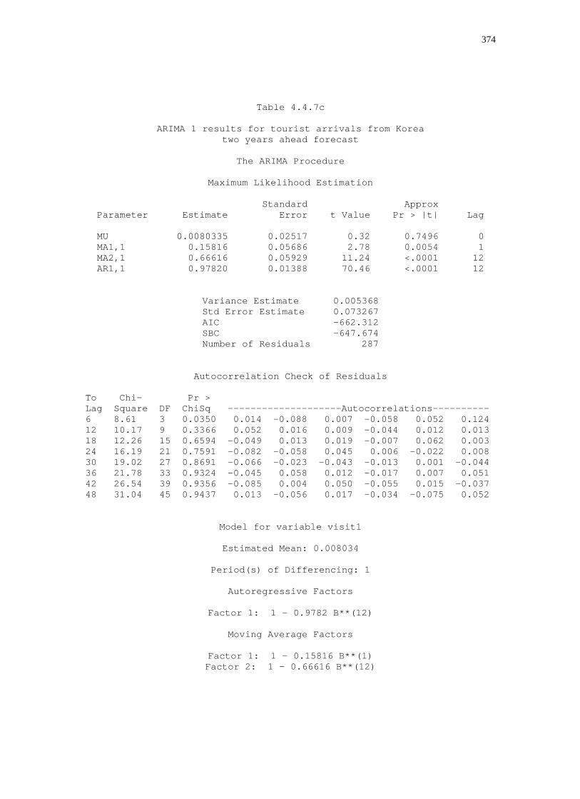
374

Table 4.4.7c

ARIMA 1 results for tourist arrivals from Korea two years ahead forecast

The ARIMA Procedure


Standard Approx


MU 0.0080335 0.02517 0.32 0.7496 0 MA1,1 0.15816 0.05686 2.78 0.0054 1 MA2,1 0.66616 0.05929 11.24 <.0001 12 AR1,1 0.97820 0.01388 70.46 <.0001 12



To Chi- Pr > Lag Square DF ChiSq --------------------Autocorrelations---------- 6 8.61 3 0.0350 0.014 -0.088 0.007 -0.058 0.052 0.124 12 10.17 9 0.3366 0.052 0.016 0.009 -0.044 0.012 0.013 18 12.26 15 0.6594 -0.049 0.013 0.019 -0.007 0.062 0.003 24 16.19 21 0.7591 -0.082 -0.058 0.045 0.006 -0.022 0.008 30 19.02 27 0.8691 -0.066 -0.023 -0.043 -0.013 0.001 -0.044 36 21.78 33 0.9324 -0.045 0.058 0.012 -0.017 0.007 0.051 42 26.54 39 0.9356 -0.085 0.004 0.050 -0.055 0.015 -0.037 48 31.04 45 0.9437 0.013 -0.056 0.017 -0.034 -0.075 0.052





Factor 1: 1 - 0.9782 B**(12)


Factor 1: 1 - 0.15816 B**(1) Factor 2: 1 - 0.66616 B**(12)

375

Table 4.4.8a

ARIMA 1 results for tourist arrivals from Singapore one month ahead forecast

The ARIMA Procedure


Standard Approx


MU 0.0075114 0.02169 0.35 0.7291 0 MA1,1 0.75141 0.03857 19.48 <.0001 1 MA2,1 0.67369 0.04982 13.52 <.0001 12 AR1,1 0.98755 0.0067452 146.41 <.0001 12



To Chi- Pr > Lag Square DF ChiSq --------------------Autocorrelations---------- 6 7.14 3 0.0677 -0.038 0.084 -0.021 0.016 -0.075 0.097 12 26.32 9 0.0018 0.082 -0.169 0.092 -0.063 0.126 -0.024 18 33.60 15 0.0039 0.123 0.032 -0.086 0.020 -0.001 0.002 24 38.17 21 0.0123 -0.014 0.010 0.028 0.045 0.097 -0.045 30 41.46 27 0.0372 0.044 0.051 0.045 -0.016 -0.056 -0.018 36 54.38 33 0.0110 -0.111 0.028 0.026 0.009 -0.017 0.159 42 59.11 39 0.0204 -0.028 0.007 -0.005 0.041 -0.095 -0.050 48 64.82 45 0.0280 -0.090 -0.051 -0.014 -0.004 0.049 -0.057





Factor 1: 1 - 0.98755 B**(12)


Factor 1: 1 - 0.75141 B**(1) Factor 2: 1 - 0.67369 B**(12)

376

Table 4.4.8b

ARIMA 1 results for tourist arrivals from Singapore one year ahead forecast

The ARIMA Procedure


Standard Approx


MU 0.01012 0.02110 0.48 0.6315 0 MA1,1 0.75650 0.03762 20.11 <.0001 1 MA2,1 0.67313 0.04936 13.64 <.0001 12 AR1,1 0.98728 0.0068256 144.64 <.0001 12



To Chi- Pr > Lag Square DF ChiSq --------------------Autocorrelations---------- 6 6.52 3 0.0890 -0.022 0.085 -0.026 -0.008 -0.087 0.073 12 23.10 9 0.0060 0.080 -0.139 0.103 -0.057 0.112 -0.037 18 29.41 15 0.0142 0.099 0.034 -0.085 0.037 -0.016 -0.019 24 34.86 21 0.0292 -0.022 -0.003 0.010 0.056 0.111 -0.026 30 37.78 27 0.0814 0.047 0.039 0.037 -0.028 -0.049 -0.023 36 51.82 33 0.0197 -0.106 0.040 0.032 0.005 -0.014 0.165 42 55.66 39 0.0407 -0.025 0.010 -0.011 0.021 -0.081 -0.056 48 62.01 45 0.0470 -0.082 -0.041 0.008 -0.015 0.041 -0.086





Factor 1: 1 - 0.98728 B**(12)


Factor 1: 1 - 0.7565 B**(1) Factor 2: 1 - 0.67313 B**(12)

377

Table 4.4.8c

ARIMA 1 results for tourist arrivals from Singapore two years ahead forecast

The ARIMA Procedure


Standard Approx


MU 0.0081199 0.02125 0.38 0.7024 0 MA1,1 0.75476 0.03825 19.73 <.0001 1 MA2,1 0.66839 0.05053 13.23 <.0001 12 AR1,1 0.98703 0.0069885 141.24 <.0001 12



To Chi- Pr > Lag Square DF ChiSq --------------------Autocorrelations---------- 6 7.44 3 0.0592 -0.034 0.085 -0.028 0.013 -0.078 0.100 12 25.71 9 0.0023 0.081 -0.169 0.092 -0.065 0.115 -0.019 18 33.36 15 0.0042 0.129 0.031 -0.084 0.020 -0.005 0.003 24 38.48 21 0.0113 -0.015 0.008 0.031 0.046 0.101 -0.052 30 41.79 27 0.0345 0.045 0.053 0.043 -0.015 -0.056 -0.017 36 53.59 33 0.0132 -0.106 0.029 0.022 0.014 -0.010 0.152 42 58.08 39 0.0252 -0.025 0.003 -0.006 0.036 -0.093 -0.052 48 63.05 45 0.0390 -0.088 -0.053 -0.017 -0.010 0.032 -0.050





Factor 1: 1 - 0.98703 B**(12)


Factor 1: 1 - 0.75476 B**(1) Factor 2: 1 - 0.66839 B**(12)

378

Table 4.4.9a

ARIMA 1 results for tourist arrivals from Taiwan one month ahead forecast

The ARIMA Procedure


Standard Approx


MU 0.0096383 0.01701 0.57 0.5709 0 MA1,1 0.67497 0.04302 15.69 <.0001 1 MA2,1 0.72685 0.05564 13.06 <.0001 12 AR1,1 0.97768 0.01229 79.53 <.0001 12



To Chi- Pr > Lag Square DF ChiSq --------------------Autocorrelations---------- 6 2.86 3 0.4130 -0.012 0.040 0.050 -0.054 -0.050 0.012 12 10.47 9 0.3136 0.032 -0.092 -0.034 -0.015 0.120 0.007 18 16.49 15 0.3501 0.074 -0.029 -0.063 -0.012 0.012 0.095 24 21.07 21 0.4544 0.057 0.072 -0.036 0.037 0.053 -0.027 30 32.05 27 0.2302 0.097 -0.079 -0.042 -0.121 0.019 0.044 36 45.77 33 0.0688 0.054 -0.019 0.098 -0.055 -0.010 0.160 42 59.23 39 0.0199 -0.171 -0.069 -0.051 0.023 -0.025 0.050 48 68.69 45 0.0130 0.030 -0.083 -0.043 -0.060 -0.015 -0.118





Factor 1: 1 - 0.97768 B**(12)


Factor 1: 1 - 0.67497 B**(1) Factor 2: 1 - 0.72685 B**(12)

379

Table 4.4.9b

ARIMA 1 results for tourist arrivals from Taiwan one year ahead forecast

The ARIMA Procedure


Standard Approx


MU 0.01047 0.01698 0.62 0.5374 0 MA1,1 0.67455 0.04223 15.97 <.0001 1 MA2,1 0.74162 0.05164 14.36 <.0001 12 AR1,1 0.98028 0.01085 90.34 <.0001 12








Factor 1: 1 - 0.98028 B**(12)


Factor 1: 1 - 0.67455 B**(1) Factor 2: 1 - 0.74162 B**(12)

380

Table 4.4.9c

ARIMA 1 results for tourist arrivals from Taiwan two years ahead forecast

The ARIMA Procedure


Standard Approx


MU 0.0094180 0.01708 0.55 0.5812 0 MA1,1 0.67507 0.04307 15.68 <.0001 1 MA2,1 0.72890 0.05568 13.09 <.0001 12 AR1,1 0.97805 0.01221 80.10 <.0001 12








Factor 1: 1 - 0.97805 B**(12)


Factor 1: 1 - 0.67507 B**(1) Factor 2: 1 - 0.7289 B**(12)

381

Table 4.4.10a

ARIMA 1 results for tourist arrivals from the UK one month ahead forecast

The ARIMA Procedure


Standard Approx


MU 0.0034701 0.01119 0.31 0.7564 0 MA1,1 0.64237 0.04461 14.40 <.0001 1 MA2,1 0.91111 0.06808 13.38 <.0001 12 AR1,1 0.99047 0.01465 67.59 <.0001 12



To Chi- Pr > Lag Square DF ChiSq --------------------Autocorrelations---------- 6 2.82 3 0.4196 -0.031 0.004 0.004 0.065 0.030 0.059 12 7.79 9 0.5552 -0.029 0.031 -0.056 0.004 0.093 -0.053 18 12.04 15 0.6763 0.082 0.039 -0.035 -0.003 0.063 0.021 24 15.31 21 0.8072 0.013 -0.079 -0.012 0.011 0.036 0.050 30 22.68 27 0.7022 0.102 0.028 0.062 0.086 -0.022 -0.009 36 43.15 33 0.1111 -0.093 0.005 -0.050 -0.104 -0.070 0.187 42 56.36 39 0.0355 -0.160 -0.109 0.037 -0.001 -0.016 -0.021 48 81.51 45 0.0007 -0.017 -0.054 -0.040 0.069 -0.023 -0.250





Factor 1: 1 - 0.99047 B**(12)


Factor 1: 1 - 0.64237 B**(1) Factor 2: 1 - 0.91111 B**(12)

382

Table 4.4.10b

ARIMA 1 results for tourist arrivals from the UK one year ahead forecast

The ARIMA Procedure


Standard Approx


MU 0.0037371 0.01049 0.36 0.7218 0 MA1,1 0.64534 0.04390 14.70 <.0001 1 MA2,1 0.89658 0.06530 13.73 <.0001 12 AR1,1 0.98572 0.01801 54.74 <.0001 12



To Chi- Pr > Lag Square DF ChiSq --------------------Autocorrelations---------- 6 2.21 3 0.5295 -0.018 -0.007 -0.006 0.063 0.036 0.040 12 7.93 9 0.5415 -0.028 0.029 -0.077 -0.009 0.087 -0.057 18 14.16 15 0.5134 0.064 0.027 -0.051 -0.046 0.070 0.073 24 18.70 21 0.6041 0.035 -0.076 -0.025 0.012 0.063 0.048 30 25.85 27 0.5269 0.099 0.026 0.052 0.080 -0.042 -0.014 36 42.65 33 0.1212 -0.085 0.012 -0.040 -0.090 -0.053 0.171 42 58.43 39 0.0235 -0.164 -0.122 0.035 -0.010 -0.040 -0.033 48 82.85 45 0.0005 -0.018 -0.019 -0.018 0.081 -0.011 -0.246





Factor 1: 1 - 0.98572 B**(12)


Factor 1: 1 - 0.64534 B**(1) Factor 2: 1 - 0.89658 B**(12)

383

Table 4.4.10c

ARIMA 1 results for tourist arrivals from the UK

two years ahead forecast

The ARIMA Procedure


Standard Approx Parameter Estimate Error t Value Pr > |t| Lag

MU 0.0032536 0.01128 0.29 0.7730 0 MA1,1 0.64164 0.04483 14.31 <.0001 1 MA2,1 0.90318 0.06896 13.10 <.0001 12 AR1,1 0.98892 0.01592 62.13 <.0001 12



To Chi- Pr > Lag Square DF ChiSq --------------------Autocorrelations---------- 6 2.97 3 0.3961 -0.031 0.003 0.002 0.068 0.032 0.059 12 8.52 9 0.4827 -0.025 0.034 -0.057 0.005 0.105 -0.049 18 12.89 15 0.6105 0.082 0.039 -0.036 -0.003 0.066 0.020 24 16.05 21 0.7667 0.013 -0.077 -0.015 0.012 0.034 0.050 30 23.82 27 0.6403 0.105 0.030 0.064 0.088 -0.023 -0.012 36 44.88 33 0.0813 -0.095 0.007 -0.049 -0.102 -0.072 0.192 42 57.47 39 0.0285 -0.158 -0.103 0.039 0.000 -0.019 -0.025 48 83.63 45 0.0004 -0.017 -0.052 -0.042 0.068 -0.017 -0.257





Factor 1: 1 - 0.98892 B**(12)


Factor 1: 1 - 0.64164 B**(1) Factor 2: 1 - 0.90318 B**(12)

384

Table 4.4.11a

ARIMA 1 results for tourist arrivals from the USA one month ahead forecast

The ARIMA Procedure


Standard Approx


MU -0.0008926 0.01116 -0.08 0.9362 0 MA1,1 0.86549 0.04672 18.53 <.0001 1 MA2,1 0.22370 0.06456 3.47 0.0005 12 AR1,1 0.49348 0.07911 6.24 <.0001 1 AR2,1 0.96836 0.01166 83.05 <.0001 12



To Chi- Pr > Lag Square DF ChiSq --------------------Autocorrelations---------- 6 11.07 2 0.0039 -0.050 0.092 0.087 -0.116 0.048 0.060 12 15.96 8 0.0429 -0.108 -0.018 -0.019 -0.061 0.018 -0.006 18 30.21 14 0.0071 -0.074 0.153 0.002 -0.042 0.112 0.057 24 46.36 20 0.0007 -0.022 0.122 0.031 -0.072 0.172 -0.015 30 55.97 26 0.0006 0.042 0.034 -0.158 0.005 0.040 -0.026 36 74.16 32 <.0001 0.022 0.171 -0.074 0.033 0.056 -0.127 42 85.99 38 <.0001 0.072 -0.031 -0.132 0.029 -0.104 -0.009 48 90.03 44 <.0001 -0.016 -0.047 -0.039 0.080 0.036 0.002


Estimated Mean: -0.00089



Factor 1: 1 - 0.49348 B**(1) Factor 2: 1 - 0.96836 B**(12)


Factor 1: 1 - 0.86549 B**(1) Factor 2: 1 - 0.2237 B**(12)

385

Table 4.4.11b

ARIMA 1 results for tourist arrivals from the USA one year ahead forecast

The ARIMA Procedure


Standard Approx


MU 0.0016035 0.01082 0.15 0.8821 0 MA1,1 0.86980 0.04368 19.91 <.0001 1 MA2,1 0.33717 0.05814 5.80 <.0001 12 AR1,1 0.50278 0.07517 6.69 <.0001 1 AR2,1 0.97439 0.0096951 100.50 <.0001 12



To Chi- Pr > Lag Square DF ChiSq --------------------Autocorrelations---------- 6 11.63 2 0.0030 -0.056 0.112 0.075 -0.118 0.020 0.051 12 16.16 8 0.0401 -0.068 -0.030 0.025 -0.090 0.019 0.006 18 30.76 14 0.0060 -0.081 0.142 0.015 -0.063 0.115 0.046 24 47.91 20 0.0004 -0.041 0.125 0.035 -0.073 0.169 -0.015 30 56.66 26 0.0005 0.029 0.041 -0.151 0.007 0.029 -0.018 36 75.36 32 <.0001 0.006 0.159 -0.084 0.015 0.076 -0.129 42 86.02 38 <.0001 0.072 -0.034 -0.121 0.030 -0.094 -0.012 48 89.31 44 <.0001 -0.012 -0.052 -0.027 0.060 0.034 -0.031





Factor 1: 1 - 0.50278 B**(1) Factor 2: 1 - 0.97439 B**(12)


Factor 1: 1 - 0.8698 B**(1) Factor 2: 1 - 0.33717 B**(12)

386

Table 4.4.11c

ARIMA 1 results for tourist arrivals from the USA two years ahead forecast

The ARIMA Procedure


Standard Approx


MU -0.0008624 0.01114 -0.08 0.9383 0 MA1,1 0.86612 0.04790 18.08 <.0001 1 MA2,1 0.22356 0.06469 3.46 0.0005 12 AR1,1 0.49444 0.08095 6.11 <.0001 1 AR2,1 0.96827 0.01170 82.77 <.0001 12



To Chi- Pr > Lag Square DF ChiSq --------------------Autocorrelations---------- 6 11.07 2 0.0039 -0.050 0.092 0.087 -0.116 0.048 0.060 12 15.92 8 0.0436 -0.108 -0.018 -0.018 -0.061 0.018 -0.006 18 30.10 14 0.0074 -0.074 0.153 0.002 -0.042 0.112 0.058 24 46.21 20 0.0008 -0.022 0.122 0.031 -0.072 0.172 -0.015 30 55.79 26 0.0006 0.042 0.034 -0.158 0.005 0.040 -0.026 36 73.93 32 <.0001 0.022 0.171 -0.074 0.033 0.056 -0.127 42 85.71 38 <.0001 0.072 -0.031 -0.132 0.029 -0.104 -0.009 48 89.71 44 <.0001 -0.016 -0.047 -0.039 0.079 0.037 0.002





Factor 1: 1 - 0.49444 B**(1) Factor 2: 1 - 0.96827 B**(12)


Factor 1: 1 - 0.86612 B**(1) Factor 2: 1 - 0.22356 B**(12)

387

Table 4.5.1a

ARIMA 1&12 results for tourist arrivals from all countries one month ahead forecast

The ARIMA Procedure


Standard Approx


MU -0.0002935 0.0005839 -0.50 0.6151 0 MA1,1 0.60261 0.04814 12.52 <.0001 1 MA2,1 0.65105 0.05182 12.56 <.0001 12



To Chi- Pr > Lag Square DF ChiSq --------------------Autocorrelations--------- 6 5.72 4 0.2207 -0.053 0.071 0.030 0.004 -0.033 0.102 12 17.72 10 0.0599 -0.078 -0.014 -0.051 -0.104 0.146 0.022 18 23.52 16 0.1004 0.003 0.078 -0.097 0.010 0.057 0.032 24 27.01 22 0.2110 -0.018 -0.030 -0.056 0.044 0.050 -0.052 30 38.66 28 0.0865 0.127 -0.104 -0.095 -0.019 -0.008 0.037 36 42.93 34 0.1402 -0.043 -0.011 -0.007 -0.042 0.011 0.098 42 50.85 40 0.1168 -0.064 -0.074 -0.098 -0.061 0.040 -0.007 48 61.33 46 0.0647 0.013 -0.063 -0.125 -0.014 0.051 -0.095



Period(s) of Differencing: 1,12


Factor 1: 1 - 0.60261 B**(1) Factor 2: 1 - 0.65105 B**(12)

388

Table 4.5.1b

ARIMA 1&12 results for tourist arrivals from all countries one year ahead forecast

The ARIMA Procedure


Standard Approx


MU -0.0002047 0.0005619 -0.36 0.7157 0 MA1,1 0.59588 0.04733 12.59 <.0001 1 MA2,1 0.66048 0.04878 13.54 <.0001 12



To Chi- Pr > Lag Square DF ChiSq --------------------Autocorrelations---------- 6 6.20 4 0.1846 -0.050 0.078 0.028 -0.014 -0.042 0.099 12 19.24 10 0.0373 -0.083 -0.019 -0.060 -0.098 0.152 0.008 18 26.98 16 0.0417 0.013 0.096 -0.109 0.007 0.060 0.021 24 30.66 22 0.1034 -0.011 -0.026 -0.065 0.047 0.053 -0.041 30 43.37 28 0.0321 0.133 -0.104 -0.094 -0.027 -0.014 0.041 36 48.62 34 0.0498 -0.044 -0.003 -0.008 -0.038 0.016 0.111 42 56.69 40 0.0420 -0.063 -0.072 -0.098 -0.064 0.037 0.005 48 67.85 46 0.0197 0.019 -0.058 -0.128 -0.014 0.046 -0.101





Factor 1: 1 - 0.59588 B**(1) Factor 2: 1 - 0.66048 B**(12)

389

Table 4.5.1c

ARIMA 1&12 results for tourist arrivals from all countries two years ahead forecast

The ARIMA Procedure


Standard Approx


MU -0.0003232 0.0005787 -0.56 0.5765 0 MA1,1 0.60402 0.04807 12.57 <.0001 1 MA2,1 0.65430 0.05176 12.64 <.0001 12



To Chi- Pr > Lag Square DF ChiSq --------------------Autocorrelations----------6 5.96 4 0.2021 -0.056 0.073 0.033 0.007 -0.031 0.103 12 18.83 10 0.0425 -0.078 -0.013 -0.052 -0.105 0.156 0.020 18 24.69 16 0.0754 0.001 0.077 -0.097 0.010 0.060 0.031 24 28.22 22 0.1686 -0.019 -0.029 -0.061 0.046 0.047 -0.050 30 39.67 28 0.0707 0.126 -0.105 -0.094 -0.019 -0.007 0.037 36 44.18 34 0.1134 -0.046 -0.013 -0.009 -0.041 0.007 0.101 42 52.08 40 0.0956 -0.066 -0.073 -0.099 -0.059 0.037 -0.009 48 62.55 46 0.0525 0.010 -0.062 -0.124 -0.012 0.055 -0.094





Factor 1: 1 - 0.60402 B**(1) Factor 2: 1 - 0.6543 B**(12)

390

Table 4.5.2a

ARIMA 1&12 results for tourist arrivals from Australia one month ahead forecast

The ARIMA Procedure


Standard Approx


MU 0.0004997 0.0010004 0.50 0.6175 0 MA1,1 0.65375 0.04576 14.29 <.0001 1 MA2,1 0.66445 0.05001 13.29 <.0001 12



To Chi- Pr > Lag Square DF ChiSq --------------------Autocorrelations--------- 6 7.86 4 0.0968 0.001 -0.089 0.113 0.038 -0.048 0.059 12 10.60 10 0.3897 0.034 -0.074 0.012 -0.030 0.040 0.015 18 19.98 16 0.2212 0.110 -0.024 -0.037 0.051 -0.033 -0.119 24 28.10 22 0.1724 0.077 0.017 -0.099 0.070 0.077 0.011 30 33.39 28 0.2217 -0.060 -0.052 -0.013 -0.030 -0.098 0.009 36 40.91 34 0.1932 -0.004 -0.127 0.024 -0.018 -0.019 0.080 42 44.60 40 0.2846 -0.072 0.053 -0.008 -0.050 0.010 0.028 48 45.72 46 0.4839 0.026 0.011 -0.030 -0.034 0.021 0.006





Factor 1: 1 - 0.65375 B**(1) Factor 2: 1 - 0.66445 B**(12)

391

Table 4.5.2b

ARIMA 1&12 results for tourist arrivals from Australia one year ahead forecast

The ARIMA Procedure


Standard Approx


MU 0.0004273 0.0009575 0.45 0.6554 0 MA1,1 0.65465 0.04475 14.63 <.0001 1 MA2,1 0.66498 0.04851 13.71 <.0001 12



To Chi- Pr > Lag Square DF ChiSq --------------------Autocorrelations--------- 6 7.65 4 0.1052 0.002 -0.087 0.110 0.033 -0.045 0.058 12 10.44 10 0.4029 0.038 -0.074 0.008 -0.027 0.037 0.016 18 20.35 16 0.2048 0.114 -0.023 -0.037 0.051 -0.032 -0.118 24 29.12 22 0.1415 0.082 0.018 -0.103 0.073 0.072 0.009 30 34.41 28 0.1878 -0.051 -0.056 -0.014 -0.025 -0.099 0.010 36 42.17 34 0.1586 -0.006 -0.126 0.024 -0.018 -0.016 0.083 42 46.48 40 0.2228 -0.074 0.056 -0.009 -0.057 0.015 0.028 48 47.76 46 0.4013 0.027 0.014 -0.033 -0.034 0.021 0.007





Factor 1: 1 - 0.65465 B**(1) Factor 2: 1 - 0.66498 B**(12)

392

Table 4.5.2c

ARIMA 1&12 results for tourist arrivals from Australia two years ahead forecast

The ARIMA Procedure


Standard Approx


MU 0.0004461 0.0010009 0.45 0.6558 0 MA1,1 0.65439 0.04573 14.31 <.0001 1 MA2,1 0.66469 0.05002 13.29 <.0001 12



To Chi- Pr > Lag Square DF ChiSq --------------------Autocorrelations---------- 6 7.84 4 0.0977 -0.002 -0.087 0.115 0.039 -0.048 0.058 12 10.59 10 0.3904 0.037 -0.073 0.011 -0.028 0.042 0.016 18 20.21 16 0.2108 0.109 -0.023 -0.037 0.053 -0.032 -0.123 24 28.59 22 0.1571 0.075 0.019 -0.102 0.074 0.077 0.011 30 33.72 28 0.2101 -0.057 -0.050 -0.014 -0.032 -0.098 0.010 36 41.40 34 0.1791 -0.004 -0.128 0.026 -0.018 -0.019 0.080 42 45.31 40 0.2602 -0.076 0.055 -0.005 -0.049 0.010 0.028 48 46.46 46 0.4534 0.027 0.014 -0.032 -0.034 0.020 0.004





Factor 1: 1 - 0.65439 B**(1) Factor 2: 1 - 0.66469 B**(12)

393

Table 4.5.3a

ARIMA 1&12 results for tourist arrivals from Canada one month ahead forecast

The ARIMA Procedure


Standard Approx


MU -0.0000556 0.0003004 -0.19 0.8531 0 MA1,1 0.91502 0.03111 29.41 <.0001 1 MA2,1 0.61975 0.05363 11.56 <.0001 12 AR1,1 0.29653 0.06856 4.32 <.0001 1



To Chi- Pr > Lag Square DF ChiSq --------------------Autocorrelations---------- 6 5.51 3 0.1382 -0.029 0.065 0.057 0.084 -0.061 0.022 12 12.05 9 0.2106 -0.020 -0.067 -0.076 -0.052 -0.080 0.053 18 25.76 15 0.0406 -0.021 0.005 -0.141 -0.104 0.039 0.116 24 33.42 21 0.0418 0.025 0.036 -0.009 0.088 0.006 0.124 30 39.56 27 0.0563 0.033 0.056 -0.097 0.062 -0.046 0.017 36 50.62 33 0.0256 0.066 0.057 -0.132 -0.019 -0.022 -0.094 42 54.28 39 0.0528 0.017 0.053 -0.085 -0.005 0.024 0.016 48 58.37 45 0.0871 0.044 0.024 0.002 0.033 -0.031 -0.087





Factor 1: 1 - 0.29653 B**(1)


Factor 1: 1 - 0.91502 B**(1) Factor 2: 1 - 0.61975 B**(12)

394

Table 4.5.3b

ARIMA 1&12 results for tourist arrivals from Canada one year ahead forecast

The ARIMA Procedure


Standard Approx


MU -0.0000855 0.0002890 -0.30 0.7673 0 MA1,1 0.91633 0.03024 30.30 <.0001 1 MA2,1 0.61797 0.05198 11.89 <.0001 12 AR1,1 0.29905 0.06676 4.48 <.0001 1



To Chi- Pr > Lag Square DF ChiSq --------------------Autocorrelations---------- 6 4.56 3 0.2069 -0.025 0.049 0.059 0.080 -0.049 0.018 12 10.56 9 0.3068 -0.021 -0.065 -0.074 -0.051 -0.065 0.056 18 24.42 15 0.0583 -0.026 0.012 -0.143 -0.104 0.038 0.108 24 32.04 21 0.0580 0.030 0.047 -0.024 0.081 0.013 0.118 30 38.56 27 0.0695 0.040 0.045 -0.098 0.069 -0.047 0.011 36 49.72 33 0.0310 0.067 0.066 -0.130 -0.019 -0.016 -0.089 42 52.99 39 0.0668 0.019 0.036 -0.079 -0.004 0.030 0.030 48 58.10 45 0.0910 0.039 0.012 0.026 0.032 -0.037 -0.100





Factor 1: 1 - 0.29905 B**(1)


Factor 1: 1 - 0.91633 B**(1) Factor 2: 1 - 0.61797 B**(12)

395

Table 4.5.3c

ARIMA 1&12 results for tourist arrivals from Canada two years ahead forecast

The ARIMA Procedure


Standard Approx


MU -0.0000651 0.0003038 -0.21 0.8303 0 MA1,1 0.91580 0.03119 29.36 <.0001 1 MA2,1 0.61660 0.05369 11.48 <.0001 12 AR1,1 0.30403 0.06857 4.43 <.0001 1



To Chi- Pr > Lag Square DF ChiSq --------------------Autocorrelations---------- 6 4.76 3 0.1906 -0.027 0.053 0.065 0.078 -0.051 0.023 12 12.04 9 0.2111 -0.019 -0.073 -0.065 -0.057 -0.089 0.066 18 26.83 15 0.0302 -0.024 0.003 -0.140 -0.109 0.038 0.129 24 33.20 21 0.0441 0.013 0.036 -0.003 0.081 0.011 0.114 30 39.61 27 0.0557 0.035 0.061 -0.098 0.062 -0.043 0.025 36 50.68 33 0.0253 0.058 0.054 -0.131 -0.019 -0.017 -0.105 42 54.20 39 0.0535 0.034 0.046 -0.085 0.009 0.018 -0.008 48 59.32 45 0.0746 0.070 0.019 0.001 0.028 -0.020 -0.095





Factor 1: 1 - 0.30403 B**(1)


Factor 1: 1 - 0.9158 B**(1) Factor 2: 1 - 0.6166 B**(12)

396

Table 4.5.4a

ARIMA 1&12 results for tourist arrivals from China one month ahead forecast

The ARIMA Procedure


Standard Approx


MU -0.0017290 0.0013028 -1.33 0.1845 0 MA1,1 0.44751 0.05364 8.34 <.0001 1 MA2,1 0.82644 0.04926 16.78 <.0001 12



To Chi- Pr > Lag Square DF ChiSq --------------------Autocorrelations--------- 6 13.23 4 0.0102 0.003 0.037 0.024 -0.154 0.051 -0.136 12 42.27 10 <.0001 0.080 0.001 0.069 0.006 -0.046 0.294 18 53.67 16 <.0001 -0.083 -0.099 -0.021 -0.084 0.055 -0.108 24 61.55 22 <.0001 0.044 -0.063 0.070 -0.035 -0.001 0.118 30 67.97 28 <.0001 -0.054 -0.001 -0.070 -0.023 -0.003 -0.111 36 78.83 34 <.0001 0.018 -0.124 0.092 0.015 -0.014 0.098 42 82.89 40 <.0001 0.000 0.045 -0.091 0.001 0.030 -0.036 48 87.39 46 0.0002 0.020 -0.064 0.003 0.016 -0.021 0.091





Factor 1: 1 - 0.44751 B**(1) Factor 2: 1 - 0.82644 B**(12)

397

Table 4.5.4b

ARIMA 1&12 results for tourist arrivals from China one year ahead forecast

The ARIMA Procedure


Standard Approx


MU -0.0016447 0.0013388 -1.23 0.2193 0 MA1,1 0.44975 0.05265 8.54 <.0001 1 MA2,1 0.80886 0.04979 16.25 <.0001 12



To Chi- Pr > Lag Square DF ChiSq --------------------Autocorrelations---------- 6 13.66 4 0.0085 0.006 0.034 0.015 -0.161 0.055 -0.127 12 42.86 10 <.0001 0.090 0.004 0.061 0.005 -0.053 0.287 18 54.08 16 <.0001 -0.076 -0.101 -0.018 -0.082 0.052 -0.104 24 61.72 22 <.0001 0.048 -0.059 0.068 -0.034 -0.009 0.113 30 67.58 28 <.0001 -0.050 0.002 -0.065 -0.028 -0.009 -0.104 36 77.63 34 <.0001 0.022 -0.116 0.090 0.005 -0.018 0.091 42 81.51 40 0.0001 0.009 0.046 -0.091 -0.001 0.022 -0.023 48 85.83 46 0.0003 0.022 -0.060 0.002 0.004 -0.023 0.089





Factor 1: 1 - 0.44975 B**(1) Factor 2: 1 - 0.80886 B**(12)

398

Table 4.5.4c

ARIMA 1&12 results for tourist arrivals from China two years ahead forecast

The ARIMA Procedure


Standard Approx


MU -0.0017723 0.0012910 -1.37 0.1698 0 MA1,1 0.44709 0.05371 8.32 <.0001 1 MA2,1 0.83020 0.04969 16.71 <.0001 12



To Chi- Pr > Lag Square DF ChiSq --------------------Autocorrelations---------- 6 13.40 4 0.0095 0.002 0.038 0.024 -0.155 0.051 -0.138 12 42.56 10 <.0001 0.080 0.002 0.068 0.006 -0.046 0.296 18 54.05 16 <.0001 -0.083 -0.098 -0.020 -0.085 0.056 -0.109 24 61.93 22 <.0001 0.044 -0.063 0.069 -0.035 -0.002 0.119 30 68.46 28 <.0001 -0.055 -0.000 -0.070 -0.023 -0.004 -0.113 36 79.30 34 <.0001 0.018 -0.124 0.093 0.015 -0.014 0.098 42 83.40 40 <.0001 0.000 0.045 -0.091 0.002 0.030 -0.038 48 88.03 46 0.0002 0.020 -0.064 0.004 0.017 -0.023 0.093





Factor 1: 1 - 0.44709 B**(1) Factor 2: 1 - 0.8302 B**(12)

399

Table 4.5.5a

ARIMA 1&12 results for tourist arrivals from France one month ahead forecast

The ARIMA Procedure


Standard Approx


MU 0.0001224 0.0005256 0.23 0.8158 0 MA1,1 0.79635 0.03708 21.48 <.0001 1 MA2,1 0.61443 0.05287 11.62 <.0001 12



To Chi- Pr > Lag Square DF ChiSq --------------------Autocorrelations---------- 6 6.10 4 0.1919 -0.010 -0.045 -0.036 0.087 0.088 -0.054 12 13.10 10 0.2183 0.021 0.097 -0.023 -0.096 0.002 0.069 18 21.52 16 0.1593 -0.063 0.084 0.049 -0.078 -0.022 -0.093 24 27.95 22 0.1772 -0.014 -0.032 -0.119 -0.043 0.000 0.064 30 40.47 28 0.0601 -0.147 -0.070 -0.048 0.043 -0.040 -0.092 36 48.25 34 0.0536 0.109 -0.044 -0.080 -0.046 0.013 0.048 42 52.84 40 0.0840 -0.070 0.003 -0.002 -0.075 -0.059 -0.007 48 62.70 46 0.0511 0.051 -0.069 0.028 0.117 0.056 -0.069





Factor 1: 1 - 0.79635 B**(1) Factor 2: 1 - 0.61443 B**(12)

400

Table 4.5.5b

ARIMA 1&12 results for tourist arrivals from France one year ahead forecast

The ARIMA Procedure


Standard Approx


MU 0.00005719 0.0005169 0.11 0.9119 0 MA1,1 0.79623 0.03646 21.84 <.0001 1 MA2,1 0.60659 0.05194 11.68 <.0001 12



To Chi- Pr > Lag Square DF ChiSq --------------------Autocorrelations---------- 6 5.58 4 0.2325 -0.009 -0.045 -0.034 0.084 0.084 -0.041 12 12.70 10 0.2410 0.016 0.092 -0.027 -0.099 0.007 0.067 18 21.03 16 0.1774 -0.061 0.085 0.046 -0.070 -0.010 -0.096 24 28.23 22 0.1682 -0.013 -0.043 -0.121 -0.044 0.002 0.067 30 40.36 28 0.0615 -0.142 -0.069 -0.047 0.036 -0.041 -0.089 36 48.17 34 0.0544 0.106 -0.044 -0.080 -0.050 0.011 0.042 42 52.87 40 0.0836 -0.072 0.008 0.003 -0.073 -0.059 -0.009 48 62.63 46 0.0518 0.047 -0.062 0.031 0.117 0.051 -0.070





Factor 1: 1 - 0.79623 B**(1) Factor 2: 1 - 0.60659 B**(12)

401

Table 4.5.5c

ARIMA 1&12 results for tourist arrivals from France two years ahead forecast

The ARIMA Procedure


Standard Approx


MU 0.0001044 0.0005247 0.20 0.8422 0 MA1,1 0.79644 0.03713 21.45 <.0001 1 MA2,1 0.61647 0.05296 11.64 <.0001 12



To Chi- Pr > Lag Square DF ChiSq --------------------Autocorrelations---------- 6 6.08 4 0.1933 -0.013 -0.043 -0.034 0.088 0.087 -0.054 12 13.10 10 0.2181 0.022 0.098 -0.023 -0.095 -0.001 0.068 18 21.44 16 0.1623 -0.061 0.083 0.050 -0.078 -0.021 -0.094 24 27.89 22 0.1794 -0.016 -0.032 -0.119 -0.044 -0.000 0.064 30 40.36 28 0.0614 -0.148 -0.069 -0.048 0.042 -0.040 -0.091 36 48.36 34 0.0524 0.110 -0.044 -0.082 -0.047 0.014 0.049 42 52.90 40 0.0832 -0.070 0.003 -0.003 -0.074 -0.059 -0.007 48 62.54 46 0.0526 0.051 -0.067 0.028 0.117 0.053 -0.068





Factor 1: 1 - 0.79644 B**(1) Factor 2: 1 - 0.61647 B**(12)

402

Table 4.5.6a

ARIMA 1&12 results for tourist arrivals from Germany one month ahead forecast

The ARIMA Procedure


Standard Approx


MU -0.0000804 0.0002713 -0.30 0.7670 0 MA1,1 0.85318 0.03174 26.88 <.0001 1 MA2,1 0.71289 0.04754 14.99 <.0001 12



To Chi- Pr > Lag Square DF ChiSq --------------------Autocorrelations---------- 6 8.41 4 0.0776 0.061 -0.030 0.021 -0.119 0.103 -0.011 12 16.48 10 0.0866 -0.087 -0.091 -0.033 0.100 0.024 -0.026 18 27.80 16 0.0334 0.156 0.027 -0.077 -0.049 -0.067 0.030 24 31.12 22 0.0936 0.006 0.023 -0.021 0.014 0.031 0.094 30 33.93 28 0.2033 -0.003 -0.057 0.004 -0.067 -0.031 -0.017 36 35.60 34 0.3930 -0.048 -0.007 -0.020 0.026 0.025 -0.036 42 42.67 40 0.3572 0.033 -0.131 -0.035 -0.009 0.021 -0.045 48 55.56 46 0.1578 -0.065 -0.011 -0.108 0.049 0.076 -0.120





Factor 1: 1 - 0.85318 B**(1) Factor 2: 1 - 0.71289 B**(12)

403

Table 4.5.6b

ARIMA 1&12 results for tourist arrivals from Germany one year ahead forecast

The ARIMA Procedure


Standard Approx


MU -0.0000585 0.0002645 -0.22 0.8249 0 MA1,1 0.86317 0.03024 28.54 <.0001 1 MA2,1 0.70043 0.04928 14.21 <.0001 12



To Chi- Pr > Lag Square DF ChiSq --------------------Autocorrelations---------- 6 9.41 4 0.0516 0.061 -0.028 0.050 -0.137 0.081 0.004 12 17.36 10 0.0667 -0.087 -0.102 -0.031 0.080 0.034 -0.014 18 29.69 16 0.0197 0.153 0.030 -0.090 -0.056 -0.058 0.041 24 33.24 22 0.0586 0.008 0.037 -0.022 -0.012 0.058 0.076 30 36.53 28 0.1297 -0.005 -0.027 -0.040 -0.079 -0.027 -0.031 36 37.79 34 0.3002 -0.031 0.014 -0.018 0.025 0.004 -0.041 42 44.47 40 0.2892 0.014 -0.132 -0.012 -0.021 0.028 -0.032 48 55.68 46 0.1553 -0.077 -0.017 -0.103 0.024 0.054 -0.111





Factor 1: 1 - 0.86317 B**(1) Factor 2: 1 - 0.70043 B**(12)

404

Table 4.5.6c

ARIMA 1&12 results for tourist arrivals from Germany two years ahead forecast

The ARIMA Procedure


Standard Approx


MU -0.0000930 0.0002737 -0.34 0.7340 0 MA1,1 0.85190 0.03206 26.58 <.0001 1 MA2,1 0.71478 0.04756 15.03 <.0001 12



To Chi- Pr > Lag Square DF ChiSq --------------------Autocorrelations---------- 6 8.51 4 0.0747 0.060 -0.031 0.024 -0.119 0.104 -0.013 12 17.01 10 0.0742 -0.089 -0.093 -0.034 0.104 0.026 -0.025 18 27.95 16 0.0320 0.154 0.027 -0.077 -0.048 -0.064 0.026 24 31.52 22 0.0860 0.005 0.022 -0.024 0.020 0.033 0.096 30 34.27 28 0.1921 -0.002 -0.057 0.003 -0.067 -0.031 -0.016 36 35.93 34 0.3781 -0.047 -0.006 -0.017 0.024 0.028 -0.037 42 42.74 40 0.3544 0.034 -0.128 -0.035 -0.007 0.023 -0.042 48 55.43 46 0.1606 -0.065 -0.008 -0.106 0.050 0.071 -0.123





Factor 1: 1 - 0.8519 B**(1) Factor 2: 1 - 0.71478 B**(12)

405

Table 4.5.7a

ARIMA 1&12 results for tourist arrivals from Korea one month ahead forecast

The ARIMA Procedure


Standard Approx


MU -0.0000895 0.0013388 -0.07 0.9467 0 MA1,1 0.13268 0.05946 2.23 0.0256 1 MA2,1 0.68266 0.05054 13.51 <.0001 12



To Chi- Pr > Lag Square DF ChiSq --------------------Autocorrelations---------- 6 8.47 4 0.0758 0.010 -0.078 -0.011 -0.055 0.047 0.136 12 10.06 10 0.4351 0.052 0.023 -0.009 -0.040 0.025 -0.004 18 11.84 16 0.7550 -0.030 0.024 -0.004 -0.008 0.066 0.013 24 14.59 22 0.8791 -0.077 -0.051 0.024 0.006 -0.005 -0.001 30 17.45 28 0.9392 -0.050 -0.013 -0.078 0.002 0.002 -0.024 36 19.92 34 0.9738 -0.016 0.064 -0.019 -0.033 0.021 0.039 42 21.40 40 0.9930 -0.041 0.004 0.015 -0.047 0.011 -0.018 48 23.58 46 0.9975 0.012 -0.063 0.006 -0.020 -0.045 -0.003





Factor 1: 1 - 0.13268 B**(1) Factor 2: 1 - 0.68266 B**(12)

406

Table 4.5.7b

ARIMA 1&12 results for tourist arrivals from Korea one year ahead forecast

The ARIMA Procedure


Standard Approx


MU -0.0002649 0.0013019 -0.20 0.8388 0 MA1,1 0.14726 0.05803 2.54 0.0112 1 MA2,1 0.67725 0.04933 13.73 <.0001 12



To Chi- Pr > Lag Square DF ChiSq --------------------Autocorrelations---------- 6 10.90 4 0.0277 0.012 -0.088 0.005 -0.070 0.040 0.151 12 13.03 10 0.2219 0.056 0.021 -0.003 -0.055 0.021 -0.005 18 14.49 16 0.5622 -0.022 0.022 -0.005 -0.007 0.060 0.009 24 16.50 22 0.7901 -0.066 -0.043 0.014 0.002 -0.010 0.002 30 19.21 28 0.8914 -0.045 -0.019 -0.075 0.000 -0.006 -0.021 36 21.50 34 0.9527 -0.006 0.062 -0.031 -0.029 0.018 0.031 42 22.74 40 0.9872 -0.031 0.005 -0.006 -0.042 0.003 -0.030 48 24.85 46 0.9954 0.022 -0.051 -0.016 -0.014 -0.042 -0.028





Factor 1: 1 - 0.14726 B**(1) Factor 2: 1 - 0.67725 B**(12)

407

Table 4.5.7c

ARIMA 1&12 results for tourist arrivals from Korea two years ahead forecast

The ARIMA Procedure


Standard Approx


MU -0.0002183 0.0013269 -0.16 0.8693 0 MA1,1 0.13871 0.05936 2.34 0.0194 1 MA2,1 0.68292 0.05041 13.55 <.0001 12



To Chi- Pr > Lag Square DF ChiSq --------------------Autocorrelations---------- 6 8.32 4 0.0805 0.011 -0.085 -0.005 -0.049 0.052 0.131 12 9.96 10 0.4438 0.054 0.022 -0.007 -0.040 0.027 -0.004 18 11.88 16 0.7521 -0.039 0.022 -0.001 -0.001 0.067 0.010 24 14.76 22 0.8725 -0.080 -0.051 0.024 0.010 -0.004 -0.006 30 17.79 28 0.9314 -0.058 -0.014 -0.075 0.003 0.002 -0.027 36 20.34 34 0.9691 -0.022 0.068 -0.019 -0.032 0.020 0.035 42 22.45 40 0.9887 -0.056 0.000 0.014 -0.053 0.010 -0.016 48 25.08 46 0.9949 0.009 -0.063 0.005 -0.027 -0.054 0.017





Factor 1: 1 - 0.13871 B**(1) Factor 2: 1 - 0.68292 B**(12)

408

Table 4.5.8a

ARIMA 1&12 results for tourist arrivals from Singapore one month ahead forecast

The ARIMA Procedure


Standard Approx


MU -0.0007641 0.0008376 -0.91 0.3617 0 MA1,1 0.74818 0.04046 18.49 <.0001 1 MA2,1 0.68807 0.04797 14.34 <.0001 12



To Chi- Pr > Lag Square DF ChiSq --------------------Autocorrelations---------- 6 6.83 4 0.1453 -0.059 0.082 -0.018 0.019 -0.088 0.075 12 27.58 10 0.0021 0.075 -0.174 0.111 -0.047 0.144 -0.031 18 34.86 16 0.0041 0.126 0.036 -0.076 0.032 -0.004 -0.029 24 40.72 22 0.0089 -0.028 -0.001 0.041 0.057 0.092 -0.071 30 43.86 28 0.0287 0.024 0.041 0.036 -0.017 -0.066 -0.043 36 56.22 34 0.0096 -0.128 0.026 0.031 0.017 -0.004 0.144 42 61.79 40 0.0151 -0.039 -0.001 -0.011 0.039 -0.094 -0.071 48 68.98 46 0.0157 -0.106 -0.050 -0.014 0.004 0.063 -0.060





Factor 1: 1 - 0.74818 B**(1) Factor 2: 1 - 0.68807 B**(12)

409

Table 4.5.8b

ARIMA 1&12 results for tourist arrivals from Singapore one year ahead forecast

The ARIMA Procedure


Standard Approx


MU -0.0004437 0.0008151 -0.54 0.5862 0 MA1,1 0.75190 0.03968 18.95 <.0001 1 MA2,1 0.68637 0.04752 14.44 <.0001 12



To Chi- Pr > Lag Square DF ChiSq --------------------Autocorrelations---------- 6 6.40 4 0.1711 -0.043 0.083 -0.023 -0.006 -0.099 0.053 12 24.42 10 0.0066 0.076 -0.141 0.121 -0.043 0.127 -0.046 18 31.41 16 0.0119 0.102 0.041 -0.074 0.051 -0.020 -0.048 24 37.74 22 0.0196 -0.033 -0.011 0.022 0.069 0.105 -0.051 30 40.60 28 0.0584 0.029 0.029 0.030 -0.029 -0.058 -0.046 36 53.99 34 0.0160 -0.121 0.040 0.038 0.012 -0.002 0.152 42 58.67 40 0.0286 -0.034 0.005 -0.017 0.019 -0.080 -0.075 48 66.24 46 0.0269 -0.095 -0.039 0.009 -0.009 0.053 -0.092





Factor 1: 1 - 0.7519 B**(1) Factor 2: 1 - 0.68637 B**(12)

410

Table 4.5.8c

ARIMA 1&12 results for tourist arrivals from Singapore two years ahead forecast

The ARIMA Procedure


Standard Approx


MU -0.0007050 0.0008382 -0.84 0.4003 0 MA1,1 0.75063 0.04023 18.66 <.0001 1 MA2,1 0.68498 0.04839 14.15 <.0001 12



To Chi- Pr > Lag Square DF ChiSq --------------------Autocorrelations---------- 6 6.99 4 0.1365 -0.056 0.083 -0.024 0.016 -0.090 0.077 12 26.79 10 0.0028 0.074 -0.174 0.111 -0.048 0.135 -0.026 18 34.39 16 0.0048 0.132 0.036 -0.074 0.032 -0.007 -0.028 24 40.85 22 0.0086 -0.030 -0.002 0.043 0.059 0.096 -0.077 30 43.97 28 0.0280 0.025 0.042 0.035 -0.016 -0.066 -0.042 36 55.53 34 0.0113 -0.125 0.026 0.028 0.021 0.003 0.138 42 60.91 40 0.0181 -0.036 -0.004 -0.012 0.035 -0.093 -0.073 48 67.26 46 0.0221 -0.105 -0.052 -0.017 -0.001 0.049 -0.053





Factor 1: 1 - 0.75063 B**(1) Factor 2: 1 - 0.68498 B**(12)

411

Table 4.5.9a

ARIMA 1&12 results for tourist arrivals from Taiwan one month ahead forecast

The ARIMA Procedure


Standard Approx


MU -0.0010912 0.0008063 -1.35 0.1759 0 MA1,1 0.68922 0.04303 16.02 <.0001 1 MA2,1 0.76412 0.04723 16.18 <.0001 12



To Chi- Pr > Lag Square DF ChiSq --------------------Autocorrelations---------- 6 2.00 4 0.7356 -0.014 0.038 0.037 -0.050 -0.030 0.026 12 9.10 10 0.5224 0.061 -0.081 -0.049 -0.029 0.105 -0.005 18 16.76 16 0.4015 0.070 -0.044 -0.095 -0.026 0.013 0.097 24 22.42 22 0.4348 0.077 0.074 -0.052 0.031 0.058 -0.023 30 35.16 28 0.1653 0.118 -0.072 -0.054 -0.124 0.030 0.055 36 49.98 34 0.0379 0.075 -0.025 0.067 -0.074 -0.009 0.174 42 62.20 40 0.0138 -0.151 -0.064 -0.078 -0.002 -0.022 0.068 48 72.08 46 0.0083 0.063 -0.082 -0.067 -0.067 -0.003 -0.100





Factor 1: 1 - 0.68922 B**(1) Factor 2: 1 - 0.76412 B**(12)

412

Table 4.5.9b

ARIMA 1&12 results for tourist arrivals from Taiwan one year ahead forecast

The ARIMA Procedure


Standard Approx


MU -0.0009152 0.0007510 -1.22 0.2230 0 MA1,1 0.68587 0.04236 16.19 <.0001 1 MA2,1 0.77604 0.04456 17.42 <.0001 12



To Chi- Pr > Lag Square DF ChiSq --------------------Autocorrelations---------- 6 2.10 4 0.7168 -0.013 0.036 0.037 -0.053 -0.028 0.028 12 9.63 10 0.4737 0.061 -0.081 -0.048 -0.027 0.109 -0.007 18 18.68 16 0.2856 0.078 -0.045 -0.114 -0.020 0.011 0.090 24 24.82 22 0.3057 0.081 0.065 -0.062 0.033 0.061 -0.015 30 38.76 28 0.0848 0.113 -0.076 -0.051 -0.134 0.031 0.059 36 54.47 34 0.0144 0.070 -0.017 0.065 -0.077 -0.008 0.180 42 68.15 40 0.0036 -0.154 -0.069 -0.074 -0.006 -0.018 0.082 48 78.09 46 0.0022 0.066 -0.076 -0.062 -0.073 -0.004 -0.098





Factor 1: 1 - 0.68587 B**(1) Factor 2: 1 - 0.77604 B**(12)

413

Table 4.5.9c

ARIMA 1&12 results for tourist arrivals from Taiwan two years ahead forecast

The ARIMA Procedure


Standard Approx


MU -0.0011263 0.0007997 -1.41 0.1590 0 MA1,1 0.69004 0.04299 16.05 <.0001 1 MA2,1 0.76680 0.04719 16.25 <.0001 12



To Chi- Pr > Lag Square DF ChiSq --------------------Autocorrelations---------- 6 1.95 4 0.7455 -0.016 0.038 0.037 -0.048 -0.028 0.028 12 9.67 10 0.4700 0.061 -0.081 -0.050 -0.030 0.114 -0.009 18 17.29 16 0.3669 0.069 -0.043 -0.095 -0.026 0.015 0.097 24 22.86 22 0.4095 0.076 0.074 -0.054 0.032 0.055 -0.018 30 35.50 28 0.1558 0.117 -0.074 -0.051 -0.124 0.032 0.055 36 50.52 34 0.0339 0.073 -0.026 0.065 -0.073 -0.012 0.178 42 62.85 40 0.0120 -0.151 -0.065 -0.079 -0.001 -0.025 0.068 48 72.65 46 0.0074 0.059 -0.082 -0.066 -0.064 0.003 -0.104





Factor 1: 1 - 0.69004 B**(1) Factor 2: 1 - 0.7668 B**(12)

414

Table 4.5.10a

ARIMA 1&12 results for tourist arrivals from the UK one month ahead forecast

The ARIMA Procedure


Standard Approx


MU -0.0009670 0.0005315 -1.82 0.0688 0 MA1,1 0.64830 0.04442 14.60 <.0001 1 MA2,1 0.93552 0.06442 14.52 <.0001 12



To Chi- Pr > Lag Square DF ChiSq --------------------Autocorrelations---------- 6 1.91 4 0.7514 -0.020 0.009 0.001 0.065 0.016 0.043 12 6.24 10 0.7948 -0.040 0.012 -0.061 0.013 0.075 -0.061 18 9.82 16 0.8759 0.063 0.070 -0.039 -0.007 0.040 0.013 24 11.89 22 0.9597 0.006 -0.065 -0.027 0.031 0.020 0.021 30 20.49 28 0.8458 0.105 0.055 0.063 0.088 -0.043 -0.018 36 40.01 34 0.2207 -0.093 0.005 -0.060 -0.103 -0.096 0.171 42 50.72 40 0.1193 -0.132 -0.110 0.043 0.000 -0.035 -0.026 48 72.71 46 0.0073 -0.002 -0.062 -0.037 0.070 -0.046 -0.231





Factor 1: 1 - 0.6483 B**(1) Factor 2: 1 - 0.93552 B**(12)

415

Table 4.5.10b

ARIMA 1&12 results for tourist arrivals from the UK one year ahead forecast

The ARIMA Procedure


Standard Approx


MU -0.0008727 0.0005308 -1.64 0.1001 0 MA1,1 0.64893 0.04361 14.88 <.0001 1 MA2,1 0.92362 0.05496 16.80 <.0001 12



To Chi- Pr > Lag Square DF ChiSq --------------------Autocorrelations---------- 6 1.64 4 0.8019 -0.007 -0.003 -0.009 0.062 0.028 0.028 12 6.88 10 0.7368 -0.037 0.011 -0.082 -0.001 0.069 -0.067 18 12.54 16 0.7059 0.041 0.051 -0.065 -0.059 0.045 0.066 24 15.88 22 0.8218 0.024 -0.069 -0.043 0.027 0.049 0.020 30 24.29 28 0.6663 0.101 0.052 0.051 0.080 -0.062 -0.024 36 39.54 34 0.2362 -0.086 0.010 -0.047 -0.087 -0.075 0.153 42 53.39 40 0.0765 -0.139 -0.123 0.039 -0.011 -0.060 -0.042 48 74.70 46 0.0047 -0.007 -0.028 -0.013 0.083 -0.033 -0.229





Factor 1: 1 - 0.64893 B**(1) Factor 2: 1 - 0.92362 B**(12)

416

Table 4.5.10c

ARIMA 1&12 results for tourist arrivals from the UK two years ahead forecast

The ARIMA Procedure


Standard Approx


MU -0.0010183 0.0005520 -1.84 0.0651 0 MA1,1 0.64764 0.04463 14.51 <.0001 1 MA2,1 0.92892 0.06159 15.08 <.0001 12



To Chi- Pr > Lag Square DF ChiSq --------------------Autocorrelations---------- 6 2.06 4 0.7245 -0.020 0.008 -0.002 0.067 0.020 0.044 12 6.83 10 0.7412 -0.036 0.016 -0.062 0.015 0.090 -0.054 18 10.50 16 0.8393 0.063 0.070 -0.040 -0.006 0.044 0.011 24 12.56 22 0.9446 0.005 -0.063 -0.032 0.032 0.018 0.022 30 21.65 28 0.7971 0.108 0.057 0.065 0.090 -0.044 -0.021 36 41.89 34 0.1659 -0.097 0.006 -0.059 -0.101 -0.097 0.177 42 51.99 40 0.0969 -0.130 -0.102 0.044 0.002 -0.037 -0.031 48 74.88 46 0.0045 -0.002 -0.060 -0.039 0.068 -0.037 -0.239





Factor 1: 1 - 0.64764 B**(1) Factor 2: 1 - 0.92892 B**(12)

417

Table 4.5.11a

ARIMA 1&12 results for tourist arrivals from the USA one month ahead forecast

The ARIMA Procedure


Standard Approx


MU -0.0001034 0.0005211 -0.20 0.8426 0 MA1,1 0.86917 0.05233 16.61 <.0001 1 MA2,1 0.75667 0.13207 5.73 <.0001 12 AR1,1 0.51642 0.08533 6.05 <.0001 1 AR2,1 0.51555 0.15808 3.26 0.0011 12



To Chi- Pr > Lag Square DF ChiSq --------------------Autocorrelations---------- 6 9.59 2 0.0083 -0.047 0.090 0.047 -0.116 0.034 0.083 12 13.58 8 0.0934 -0.098 0.014 -0.043 -0.038 0.028 -0.000 18 23.25 14 0.0564 -0.044 0.140 -0.037 -0.051 0.066 0.054 24 36.56 20 0.0132 -0.034 0.086 0.021 -0.059 0.166 0.063 30 46.04 26 0.0090 0.042 0.053 -0.156 0.011 0.035 -0.025 36 60.90 32 0.0015 -0.003 0.159 -0.080 0.034 0.057 -0.105 42 71.52 38 0.0008 0.065 -0.015 -0.129 0.022 -0.105 0.006 48 77.37 44 0.0014 -0.038 -0.045 -0.078 0.067 0.058 0.016





Factor 1: 1 - 0.51642 B**(1) Factor 2: 1 - 0.51555 B**(12)


Factor 1: 1 - 0.86917 B**(1) Factor 2: 1 - 0.75667 B**(12)

418

Table 4.5.11b

ARIMA 1&12 results for tourist arrivals from the USA one year ahead forecast

The ARIMA Procedure


Standard Approx


MU 0.00004960 0.0004326 0.11 0.9087 0 MA1,1 0.88081 0.04720 18.66 <.0001 1 MA2,1 0.75398 0.10192 7.40 <.0001 12 AR1,1 0.53734 0.07909 6.79 <.0001 1 AR2,1 0.43644 0.13016 3.35 0.0008 12



To Chi- Pr > Lag Square DF ChiSq --------------------Autocorrelations---------- 6 10.34 2 0.0057 -0.054 0.109 0.037 -0.115 0.001 0.077 12 12.73 8 0.1213 -0.051 0.004 -0.003 -0.067 0.030 -0.005 18 21.67 14 0.0856 -0.038 0.126 -0.019 -0.072 0.068 0.043 24 35.49 20 0.0177 -0.041 0.086 0.030 -0.060 0.158 0.074 30 43.55 26 0.0169 0.038 0.054 -0.141 0.010 0.023 -0.018 36 57.57 32 0.0037 -0.010 0.145 -0.089 0.019 0.072 -0.090 42 66.14 38 0.0031 0.064 -0.015 -0.109 0.019 -0.095 0.008 48 70.28 44 0.0071 -0.033 -0.048 -0.059 0.045 0.056 -0.003





Factor 1: 1 - 0.53734 B**(1) Factor 2: 1 - 0.43644 B**(12)


Factor 1: 1 - 0.88081 B**(1) Factor 2: 1 - 0.75398 B**(12)

419

Table 4.5.11c

ARIMA 1&12 results for tourist arrivals from the USA two years ahead forecast

The ARIMA Procedure


Standard Approx


MU -0.0000987 0.0005189 -0.19 0.8491 0 MA1,1 0.87091 0.05341 16.31 <.0001 1 MA2,1 0.75735 0.13179 5.75 <.0001 12 AR1,1 0.51911 0.08720 5.95 <.0001 1 AR2,1 0.51610 0.15794 3.27 0.0011 12



To Chi- Pr > Lag Square DF ChiSq --------------------Autocorrelations---------- 6 9.69 2 0.0079 -0.046 0.090 0.047 -0.119 0.035 0.083 12 13.58 8 0.0933 -0.097 0.014 -0.042 -0.038 0.028 -0.000 18 23.20 14 0.0571 -0.043 0.141 -0.037 -0.051 0.066 0.054 24 36.51 20 0.0134 -0.033 0.086 0.021 -0.059 0.166 0.063 30 46.01 26 0.0091 0.042 0.053 -0.156 0.011 0.035 -0.025 36 60.84 32 0.0016 -0.002 0.159 -0.080 0.035 0.056 -0.105 42 71.41 38 0.0008 0.065 -0.015 -0.129 0.022 -0.106 0.007 48 77.22 44 0.0015 -0.038 -0.044 -0.078 0.066 0.059 0.016





Factor 1: 1 - 0.51911 B**(1) Factor 2: 1 - 0.5161 B**(12)


Factor 1: 1 - 0.87091 B**(1) Factor 2: 1 - 0.75735 B**(12)

420

Table 4.6.1a

BSM results for tourist arrivals from all countries one month ahead forecast

Method of estimation is Maximum likelihood The present sample is: 1978 (1) to 2003 (12) less 23 forecasts

Equation Larr = Trend + Trigo seasonal + Irregular Estimation report Model with 4 parameters ( 1 restrictions). Parameter estimation sample is 1978. 1 - 2002. 1. (T = 289). Log-likelihood kernel is 2.561141. Very strong convergence in 7 iterations. ( likelihood cvg 4.662593e-013 gradient cvg 1.489179e-008 parameter cvg 1.683058e-006 ) Diagnostic summary report. Estimation sample is 1978. 1 - 2002. 1. (T = 289, n = 276). Log-Likelihood is 740.17 (-2 LogL = -1480.34). Prediction error variance is 0.00393811 Summary statistics Larr Std.Error 0.062754 Normality 24.194 H( 92) 0.55737 r( 1) -0.026883 r(16) 0.0032611 DW 2.0414 Q(16,13) 22.622 Rs^2 0.31582 Estimated variances of disturbances. Component Larr (q-ratio) Irr 0.0015021 ( 1.0000) Lvl 0.00048142 ( 0.3205) Slp 7.7695e-008 ( 0.0001) Sea 5.7824e-006 ( 0.0038)

421

Table 4.6.1b

BSM results for tourist arrivals from all countries one year ahead forecast

Method of estimation is Maximum likelihood The present sample is: 1978 (1) to 2003 (12) less 12 forecasts Equation Larr = Trend + Trigo seasonal + Irregular Estimation report Model with 4 parameters ( 2 restrictions). Parameter estimation sample is 1978. 1 - 2002.12. (T = 300). Log-likelihood kernel is 2.575637. Very strong convergence in 9 iterations. ( likelihood cvg 1.245039e-012 gradient cvg 2.426948e-008 parameter cvg 2.982662e-006 ) Diagnostic summary report. Estimation sample is 1978. 1 - 2002.12. (T = 300, n = 287). Log-Likelihood is 772.691 (-2 LogL = -1545.38). Prediction error variance is 0.00385487 Summary statistics Larr Std.Error 0.062088 Normality 26.605 H( 95) 0.59653 r( 1) -0.024028 r(16) 0.0010471 DW 2.0318 Q(16,13) 26.816 Rs^2 0.32562 Estimated variances of disturbances. Component Larr (q-ratio) Irr 0.0014886 ( 1.0000) Lvl 0.00050585 ( 0.3398) Slp 0.00000 ( 0.0000) Sea 5.3090e-006 ( 0.0036)

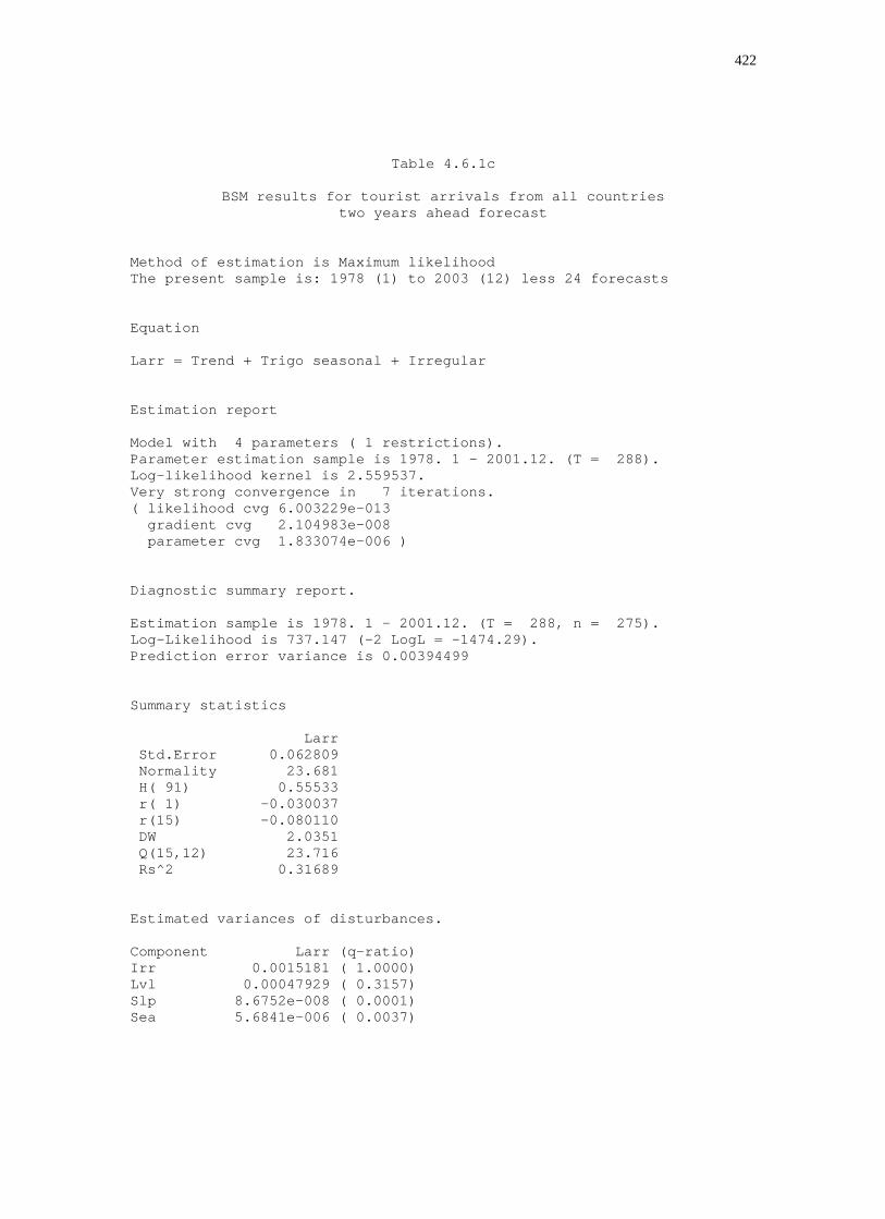
422

Table 4.6.1c

BSM results for tourist arrivals from all countries two years ahead forecast


Equation Larr = Trend + Trigo seasonal + Irregular Estimation report Model with 4 parameters ( 1 restrictions). Parameter estimation sample is 1978. 1 - 2001.12. (T = 288). Log-likelihood kernel is 2.559537. Very strong convergence in 7 iterations. ( likelihood cvg 6.003229e-013 gradient cvg 2.104983e-008 parameter cvg 1.833074e-006 ) Diagnostic summary report. Estimation sample is 1978. 1 - 2001.12. (T = 288, n = 275). Log-Likelihood is 737.147 (-2 LogL = -1474.29). Prediction error variance is 0.00394499 Summary statistics Larr Std.Error 0.062809 Normality 23.681 H( 91) 0.55533 r( 1) -0.030037 r(15) -0.080110 DW 2.0351 Q(15,12) 23.716 Rs^2 0.31689 Estimated variances of disturbances. Component Larr (q-ratio) Irr 0.0015181 ( 1.0000) Lvl 0.00047929 ( 0.3157) Slp 8.6752e-008 ( 0.0001) Sea 5.6841e-006 ( 0.0037)

423

Table 4.6.2a

BSM results for tourist arrivals from Australia one month ahead forecast


Equation Larr = Trend + Trigo seasonal + Irregular Estimation report Model with 4 parameters ( 2 restrictions). Parameter estimation sample is 1978. 1 - 2002. 1. (T = 289). Log-likelihood kernel is 1.883547. Very strong convergence in 7 iterations. ( likelihood cvg 7.073184e-016 gradient cvg 3.993139e-007 parameter cvg 2.66798e-010 ) Diagnostic summary report. Estimation sample is 1978. 1 - 2002. 1. (T = 289, n = 276). Log-Likelihood is 544.345 (-2 LogL = -1088.69). Prediction error variance is 0.0161302 Summary statistics Larr Std.Error 0.12700 Normality 31.926 H( 92) 0.22760 r( 1) 0.0090518 r(16) 0.046302 DW 1.9613 Q(16,13) 17.148 Rs^2 0.42994 Estimated variances of disturbances. Component Larr (q-ratio) Irr 0.0071505 ( 1.0000) Lvl 0.0015803 ( 0.2210) Slp 0.00000 ( 0.0000) Sea 2.0716e-005 ( 0.0029)

424

Table 4.6.2b

BSM results for tourist arrivals from Australia one year ahead forecast

Method of estimation is Maximum likelihood The present sample is: 1978 (1) to 2003 (12) less 12 forecasts Equation Larr = Trend + Trigo seasonal + Irregular Estimation report Model with 4 parameters ( 2 restrictions). Parameter estimation sample is 1978. 1 - 2002.12. (T = 300). Log-likelihood kernel is 1.905065. Very strong convergence in 8 iterations. ( likelihood cvg 3.496647e-015 gradient cvg 1.40632e-007 parameter cvg 3.436338e-011 ) Diagnostic summary report. Estimation sample is 1978. 1 - 2002.12. (T = 300, n = 287). Log-Likelihood is 571.519 (-2 LogL = -1143.04). Prediction error variance is 0.0156307 Summary statistics Larr Std.Error 0.12502 Normality 35.708 H( 95) 0.22797 r( 1) 0.010459 r(16) 0.047020 DW 1.9620 Q(16,13) 17.532 Rs^2 0.43736 Estimated variances of disturbances. Component Larr (q-ratio) Irr 0.0069409 ( 1.0000) Lvl 0.0015212 ( 0.2192) Slp 0.00000 ( 0.0000) Sea 1.9928e-005 ( 0.0029)

425

Table 4.6.2c

BSM results for tourist arrivals from Australia two years ahead forecast


Equation Larr = Trend + Trigo seasonal + Irregular Estimation report Model with 4 parameters ( 2 restrictions). Parameter estimation sample is 1978. 1 - 2001.12. (T = 288). Log-likelihood kernel is 1.882663. Very strong convergence in 8 iterations. ( likelihood cvg 9.175988e-012 gradient cvg 2.83118e-007 parameter cvg 5.191441e-006 ) Diagnostic summary report. Estimation sample is 1978. 1 - 2001.12. (T = 288, n = 275). Log-Likelihood is 542.207 (-2 LogL = -1084.41). Prediction error variance is 0.016138 Summary statistics Larr Std.Error 0.12704 Normality 31.731 H( 91) 0.22761 r( 1) 0.0063616 r(15) -0.036342 DW 1.9648 Q(15,12) 16.382 Rs^2 0.43136 Estimated variances of disturbances. Component Larr (q-ratio) Irr 0.0071741 ( 1.0000) Lvl 0.0015751 ( 0.2196) Slp 0.00000 ( 0.0000) Sea 2.0641e-005 ( 0.0029)

426

Table 4.6.3a

BSM results for tourist arrivals from Canada one month ahead forecast


Equation Larr = Trend + Trigo seasonal + Irregular Estimation report Model with 4 parameters ( 2 restrictions). Parameter estimation sample is 1978. 1 - 2002. 1. (T = 289). Log-likelihood kernel is 2.162498. Very strong convergence in 8 iterations. ( likelihood cvg 1.437516e-015 gradient cvg 2.300826e-007 parameter cvg 5.223337e-012 ) Diagnostic summary report. Estimation sample is 1978. 1 - 2002. 1. (T = 289, n = 276). Log-Likelihood is 624.962 (-2 LogL = -1249.92). Prediction error variance is 0.00904529 Summary statistics Larr Std.Error 0.095107 Normality 13.498 H( 92) 0.75907 r( 1) 0.080651 r(16) -0.15162 DW 1.8363 Q(16,13) 28.900 Rs^2 0.32771 Estimated variances of disturbances. Component Larr (q-ratio) Irr 0.0035979 ( 1.0000) Lvl 0.00078363 ( 0.2178) Slp 0.00000 ( 0.0000) Sea 1.7359e-005 ( 0.0048)

427

Table 4.6.3b

BSM results for tourist arrivals from Canada one year ahead forecast

Method of estimation is Maximum likelihood The present sample is: 1978 (1) to 2003 (12) less 12 forecasts Equation Larr = Trend + Trigo seasonal + Irregular Estimation report Model with 4 parameters ( 2 restrictions). Parameter estimation sample is 1978. 1 - 2002.12. (T = 300). Log-likelihood kernel is 2.171997. Very strong convergence in 8 iterations. ( likelihood cvg 3.291826e-013 gradient cvg 6.972201e-009 parameter cvg 3.349056e-007 ) Diagnostic summary report. Estimation sample is 1978. 1 - 2002.12. (T = 300, n = 287). Log-Likelihood is 651.599 (-2 LogL = -1303.2). Prediction error variance is 0.00899141 Summary statistics Larr Std.Error 0.094823 Normality 12.775 H( 95) 0.80854 r( 1) 0.091644 r(16) -0.14706 DW 1.8138 Q(16,13) 29.867 Rs^2 0.33723 Estimated variances of disturbances. Component Larr (q-ratio) Irr 0.0036891 ( 1.0000) Lvl 0.00072636 ( 0.1969) Slp 0.00000 ( 0.0000) Sea 1.6823e-005 ( 0.0046)

428

Table 4.6.3c

BSM results for tourist arrivals from Canada two years ahead forecast



429

Table 4.6.4a

BSM results for tourist arrivals from China

one month ahead forecast


Equation Larr = Trend + Trigo seasonal + Irregular Estimation report Model with 4 parameters ( 1 restrictions). Parameter estimation sample is 1978. 1 - 2002. 1. (T = 289). Log-likelihood kernel is 1.573883. Very strong convergence in 6 iterations. ( likelihood cvg 4.919486e-013 gradient cvg 3.251473e-008 parameter cvg 4.170549e-006 ) Diagnostic summary report. Estimation sample is 1978. 1 - 2002. 1. (T = 289, n = 276). Log-Likelihood is 454.852 (-2 LogL = -909.704). Prediction error variance is 0.0305326 Summary statistics Larr Std.Error 0.17474 Normality 143.57 H( 92) 0.098132 r( 1) -0.00048033 r(16) -0.092322 DW 1.9026 Q(16,13) 49.172 Rs^2 0.084193 Estimated variances of disturbances. Component Larr (q-ratio) Irr 0.010916 ( 1.0000) Lvl 0.0083517 ( 0.7651) Slp 1.8363e-006 ( 0.0002) Sea 1.1727e-005 ( 0.0011)

430

Table 4.6.4b

BSM results for tourist arrivals from China one year ahead forecast

Method of estimation is Maximum likelihood The present sample is: 1978 (1) to 2003 (12) less 12 forecasts Equation Larr = Trend + Trigo seasonal + Irregular Estimation report Model with 4 parameters ( 1 restrictions). Parameter estimation sample is 1978. 1 - 2002.12. (T = 300). Log-likelihood kernel is 1.585868. Very strong convergence in 5 iterations. ( likelihood cvg 9.157093e-012 gradient cvg 1.714776e-007 parameter cvg 7.571981e-006 ) Diagnostic summary report. Estimation sample is 1978. 1 - 2002.12. (T = 300, n = 287). Log-Likelihood is 475.76 (-2 LogL = -951.521). Prediction error variance is 0.030291 Summary statistics Larr Std.Error 0.17404 Normality 154.09 H( 95) 0.12025 r( 1) 0.0022841 r(16) -0.088404 DW 1.8988 Q(16,13) 48.478 Rs^2 0.091767 Estimated variances of disturbances. Component Larr (q-ratio) Irr 0.010373 ( 1.0000) Lvl 0.0081064 ( 0.7815) Slp 1.6632e-006 ( 0.0002) Sea 1.5099e-005 ( 0.0015)

431

Table 4.6.4c

BSM results for tourist arrivals from China two years ahead forecast



432

Table 4.6.5a

BSM results for tourist arrivals from France




433

Table 4.6.5b

BSM results for tourist arrivals from France one year ahead forecast


434

Table 4.6.5c

BSM results for tourist arrivals from France two years ahead forecast


Equation Larr = Trend + Trigo seasonal + Irregular Estimation report Model with 4 parameters ( 2 restrictions). Parameter estimation sample is 1978. 1 - 2001.12. (T = 288). Log-likelihood kernel is 2.123663. Very strong convergence in 7 iterations. ( likelihood cvg 9.520783e-012 gradient cvg 1.462608e-007 parameter cvg 5.752388e-006 ) Diagnostic summary report. Estimation sample is 1978. 1 - 2001.12. (T = 288, n = 275). Log-Likelihood is 611.615 (-2 LogL = -1223.23). Prediction error variance is 0.00977148 Summary statistics Larr Std.Error 0.098851 Normality 23.086 H( 91) 0.25834 r( 1) -0.0015101 r(15) 0.066484 DW 1.9517 Q(15,12) 17.355 Rs^2 0.49881 Estimated variances of disturbances. Component Larr (q-ratio) Irr 0.0048549 ( 1.0000) Lvl 0.00033699 ( 0.0694) Slp 0.00000 ( 0.0000) Sea 1.9077e-005 ( 0.0039)

435

Table 4.6.6a

BSM results for tourist arrivals from Germany




436

Table 4.6.6b

BSM results for tourist arrivals from Germany one year ahead forecast


437

Table 4.6.6c

BSM results for tourist arrivals from Germany two years ahead forecast



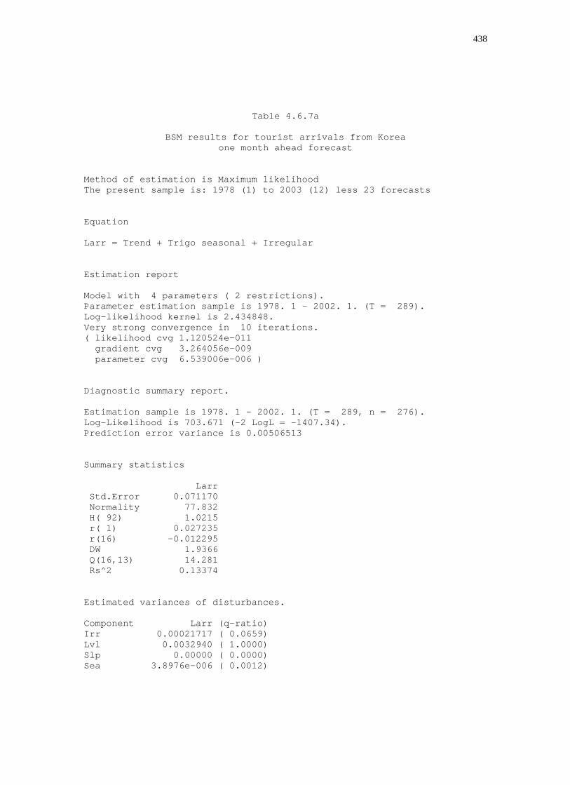
438

Table 4.6.7a

BSM results for tourist arrivals from Korea




439

Table 4.6.7b

BSM results for tourist arrivals from Korea one year ahead forecast


440

Table 4.6.7c

BSM results for tourist arrivals from Korea two years ahead forecast



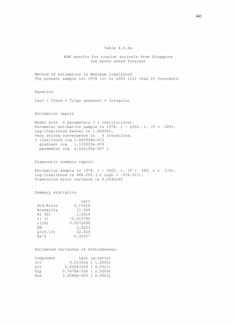
441

Table 4.6.8a

BSM results for tourist arrivals from Singapore



Equation Larr = Trend + Trigo seasonal + Irregular Estimation report Model with 4 parameters ( 1 restrictions). Parameter estimation sample is 1978. 1 - 2002. 1. (T = 289). Log-likelihood kernel is 1.689465. Very strong convergence in 6 iterations. ( likelihood cvg 1.843949e-013 gradient cvg 1.102822e-009 parameter cvg 6.582105e-007 ) Diagnostic summary report. Estimation sample is 1978. 1 - 2002. 1. (T = 289, n = 276). Log-Likelihood is 488.255 (-2 LogL = -976.511). Prediction error variance is 0.0244165 Summary statistics Larr Std.Error 0.15626 Normality 11.666 H( 92) 1.0515 r( 1) -0.013790 r(16) 0.0072498 DW 2.0223 Q(16,13) 32.520 Rs^2 0.32327 Estimated variances of disturbances. Component Larr (q-ratio) Irr 0.013526 ( 1.0000) Lvl 0.00043356 ( 0.0321) Slp 5.7478e-006 ( 0.0004) Sea 2.9288e-005 ( 0.0022)

442

Table 4.6.8b

BSM results for tourist arrivals from Singapore one year ahead forecast

Method of estimation is Maximum likelihood The present sample is: 1978 (1) to 2003 (12) less 12 forecasts Equation Larr = Trend + Trigo seasonal + Irregular Estimation report Model with 4 parameters ( 1 restrictions). Parameter estimation sample is 1978. 1 - 2002.12. (T = 300). Log-likelihood kernel is 1.687628. Very strong convergence in 7 iterations. ( likelihood cvg 7.016733e-013 gradient cvg 6.757557e-009 parameter cvg 6.203056e-007 ) Diagnostic summary report. Estimation sample is 1978. 1 - 2002.12. (T = 300, n = 287). Log-Likelihood is 506.289 (-2 LogL = -1012.58). Prediction error variance is 0.0248105 Summary statistics Larr Std.Error 0.15751 Normality 9.5371 H( 95) 1.0890 r( 1) -0.0051355 r(16) 0.034637 DW 2.0062 Q(16,13) 29.621 Rs^2 0.32823 Estimated variances of disturbances. Component Larr (q-ratio) Irr 0.013512 ( 1.0000) Lvl 0.00068651 ( 0.0508) Slp 3.1152e-006 ( 0.0002) Sea 3.0004e-005 ( 0.0022)

443

Table 4.6.8c

BSM results for tourist arrivals from Singapore two years ahead forecast



444

Table 4.6.9a

BSM results for tourist arrivals from Taiwan



Equation Larr = Trend + Trigo seasonal + Irregular Estimation report Model with 4 parameters ( 2 restrictions). Parameter estimation sample is 1978. 1 - 2002. 1. (T = 289). Log-likelihood kernel is 1.684258. Very strong convergence in 9 iterations. ( likelihood cvg 9.604199e-013 gradient cvg 4.074519e-009 parameter cvg 3.958752e-006 ) Diagnostic summary report. Estimation sample is 1978. 1 - 2002. 1. (T = 289, n = 276). Log-Likelihood is 486.751 (-2 LogL = -973.501). Prediction error variance is 0.0224342 Summary statistics Larr Std.Error 0.14978 Normality 12.930 H( 92) 0.86767 r( 1) 0.023855 r(16) -0.035201 DW 1.9422 Q(16,13) 24.668 Rs^2 0.31243 Estimated variances of disturbances. Component Larr (q-ratio) Irr 0.016636 ( 1.0000) Lvl 0.0014753 ( 0.0887) Slp 2.7912e-006 ( 0.0002) Sea 0.00000 ( 0.0000)

445

Table 4.6.9b

BSM results for tourist arrivals from Taiwan one year ahead forecast

Method of estimation is Maximum likelihood The present sample is: 1978 (1) to 2003 (12) less 12 forecasts Equation Larr = Trend + Trigo seasonal + Irregular Estimation report Model with 4 parameters ( 2 restrictions). Parameter estimation sample is 1978. 1 - 2002.12. (T = 300). Log-likelihood kernel is 1.704772. Very strong convergence in 10 iterations. ( likelihood cvg 1.953732e-015 gradient cvg 1.154632e-008 parameter cvg 2.169434e-009 ) Diagnostic summary report. Estimation sample is 1978. 1 - 2002.12. (T = 300, n = 287). Log-Likelihood is 511.432 (-2 LogL = -1022.86). Prediction error variance is 0.0218124 Summary statistics Larr Std.Error 0.14769 Normality 14.505 H( 95) 0.85477 r( 1) 0.024548 r(16) -0.039268 DW 1.9447 Q(16,13) 27.562 Rs^2 0.31056 Estimated variances of disturbances. Component Larr (q-ratio) Irr 0.016044 ( 1.0000) Lvl 0.0015297 ( 0.0953) Slp 2.2887e-006 ( 0.0001) Sea 0.00000 ( 0.0000)

446

Table 4.6.9c

BSM results for tourist arrivals from Taiwan two years ahead forecast


Equation Larr = Trend + Trigo seasonal + Irregular Estimation report Model with 4 parameters ( 2 restrictions). Parameter estimation sample is 1978. 1 - 2001.12. (T = 288). Log-likelihood kernel is 1.683422. Very strong convergence in 7 iterations. ( likelihood cvg 1.631612e-012 gradient cvg 1.280087e-008 parameter cvg 3.260192e-006 ) Diagnostic summary report. Estimation sample is 1978. 1 - 2001.12. (T = 288, n = 275). Log-Likelihood is 484.825 (-2 LogL = -969.651). Prediction error variance is 0.0224458 Summary statistics Larr Std.Error 0.14982 Normality 13.075 H( 91) 0.86223 r( 1) 0.023706 r(15) -0.13040 DW 1.9435 Q(15,12) 23.915 Rs^2 0.31427 Estimated variances of disturbances. Component Larr (q-ratio) Irr 0.016715 ( 1.0000) Lvl 0.0014107 ( 0.0844) Slp 3.1278e-006 ( 0.0002) Sea 0.00000 ( 0.0000)

447

Table 4.6.10a

BSM results for tourist arrivals from the UK



Equation Larr = Trend + Trigo seasonal + Irregular Estimation report Model with 4 parameters ( 2 restrictions). Parameter estimation sample is 1978. 1 - 2002. 1. (T = 289). Log-likelihood kernel is 1.624104. Very strong convergence in 10 iterations. ( likelihood cvg 6.499586e-013 gradient cvg 8.881784e-010 parameter cvg 3.327675e-006 ) Diagnostic summary report. Estimation sample is 1978. 1 - 2002. 1. (T = 289, n = 276). Log-Likelihood is 469.366 (-2 LogL = -938.732). Prediction error variance is 0.025462 Summary statistics Larr Std.Error 0.15957 Normality 37.537 H( 92) 1.1287 r( 1) -0.0090781 r(16) -0.014219 DW 1.9742 Q(16,13) 8.0366 Rs^2 0.30440 Estimated variances of disturbances. Component Larr (q-ratio) Irr 0.017381 ( 1.0000) Lvl 0.0025113 ( 0.1445) Slp 5.0142e-006 ( 0.0003) Sea 0.00000 ( 0.0000)

448

Table 4.6.10b

BSM results for tourist arrivals from the UK one year ahead forecast

Method of estimation is Maximum likelihood The present sample is: 1978 (1) to 2003 (12) less 12 forecasts Equation Larr = Trend + Trigo seasonal + Irregular Estimation report Model with 4 parameters ( 3 restrictions). Parameter estimation sample is 1978. 1 - 2002.12. (T = 300). Log-likelihood kernel is 1.616424. Very strong convergence in 11 iterations. ( likelihood cvg 2.828541e-012 gradient cvg 6.883383e-010 parameter cvg 5.566104e-006 ) Diagnostic summary report. Estimation sample is 1978. 1 - 2002.12. (T = 300, n = 287). Log-Likelihood is 484.927 (-2 LogL = -969.854). Prediction error variance is 0.0260202 Summary statistics Larr Std.Error 0.16131 Normality 37.675 H( 95) 1.2615 r( 1) -0.017403 r(16) -0.061289 DW 1.9846 Q(16,13) 9.0585 Rs^2 0.30025 Estimated variances of disturbances. Component Larr (q-ratio) Irr 0.017115 ( 1.0000) Lvl 0.0036079 ( 0.2108) Slp 0.00000 ( 0.0000) Sea 0.00000 ( 0.0000)

449

Table 4.6.10c

BSM results for tourist arrivals from the UK two years ahead forecast



450

Table 4.6.11a

BSM results for tourist arrivals from the USA




451

Table 4.6.11b

BSM results for tourist arrivals from the USA one year ahead forecast


452

Table 4.6.11c

BSM results for tourist arrivals from the USA two years ahead forecast


APPENDIX II

Appendix to Chapter 5

454

Table 5.4.1a Microfit output for ECM Arrivals from All Countries, one month ahead model Estimated Cointegrated Vectors in Johansen Estimation (Normalized in Brackets) Cointegration with no intercepts or trends in the VAR ****************************************************************************** 288 observations from 1978M2 to 2002M1 . Order of VAR = 1, chosen r =1. List of variables included in the cointegrating vector: ARR IMPJAP ****************************************************************************** Vector 1 ARR -.15796 ( -1.0000) IMPJAP .24872 ( 1.5746) ****************************************************************************** Ordinary Least Squares Estimation ****************************************************************************** Dependent variable is DARR 288 observations used for estimation from 1978M2 to 2002M1 ****************************************************************************** Regressor Coefficient Standard Error T-Ratio[Prob] CONST .037614 .015937 2.3602[.019] S2 -.059397 .022152 -2.6814[.008] S3 .10881 .022148 4.9127[.000] S4 .10332 .022234 4.6469[.000] S5 -.071246 .022495 -3.1672[.002] S6 -.10586 .022368 -4.7326[.000] S7 .11529 .022278 5.1749[.000] S8 -.075927 .022595 -3.3603[.001] S9 -.10337 .022451 -4.6043[.000] S10 .11746 .022335 5.2587[.000] S11 -.21747 .022639 -9.6060[.000] S12 -.20169 .022256 -9.0623[.000] UT(-1) -.033191 .012901 -2.5727[.011] ****************************************************************************** R-Squared .71389 R-Bar-Squared .70140 S.E. of Regression .076723 F-stat. F( 12, 275) 57.1801[.000] Mean of Dependent Variable .0063225 S.D. of Dependent Variable .14040 Residual Sum of Squares 1.6188 Equation Log-likelihood 337.4534 Akaike Info. Criterion 324.4534 Schwarz Bayesian Criterion 300.6442 DW-statistic 2.6006 ******************************************************************************

455

Table 5.4.1b Microfit output for ECM Arrivals from All Countries, 12 months ahead model Estimated Cointegrated Vectors in Johansen Estimation (Normalized in Brackets) Cointegration with no intercepts or trends in the VAR ****************************************************************************** 299 observations from 1978M2 to 2002M12. Order of VAR = 1, chosen r =1. List of variables included in the cointegrating vector: ARR IMPJAP ****************************************************************************** Vector 1 ARR -.15720 ( -1.0000) IMPJAP .24753 ( 1.5746) ****************************************************************************** Ordinary Least Squares Estimation ****************************************************************************** Dependent variable is DARR 299 observations used for estimation from 1978M2 to 2002M12 ****************************************************************************** Regressor Coefficient Standard Error T-Ratio[Prob] CONST .037317 .015853 2.3539[.019] S2 -.057647 .021821 -2.6418[.009] S3 .10628 .021815 4.8719[.000] S4 .10059 .021916 4.5899[.000] S5 -.071210 .022168 -3.2123[.001] S6 -.10248 .022038 -4.6499[.000] S7 .11605 .021961 5.2841[.000] S8 -.076004 .022280 -3.4114[.001] S9 -.10754 .022135 -4.8584[.000] S10 .11802 .022002 5.3642[.000] S11 -.21573 .022306 -9.6715[.000] S12 -.19605 .021923 -8.9428[.000] UT(-1) -.034489 .012759 -2.7030[.007] ****************************************************************************** R-Squared .71195 R-Bar-Squared .69986 S.E. of Regression .076335 F-stat. F( 12, 286) 58.9070[.000] Mean of Dependent Variable .0060992 S.D. of Dependent Variable .13934 Residual Sum of Squares 1.6665 Equation Log-likelihood 351.5957 Akaike Info. Criterion 338.5957 Schwarz Bayesian Criterion 314.5429 DW-statistic 2.5597 ******************************************************************************

456

Table 5.4.1c Microfit output for ECM Arrivals from All Countries, 24 months ahead model Estimated Cointegrated Vectors in Johansen Estimation (Normalized in Brackets) Cointegration with no intercepts or trends in the VAR ****************************************************************************** 287 observations from 1978M2 to 2001M12. Order of VAR = 1, chosen r =1. List of variables included in the cointegrating vector: ARR IMPJAP ****************************************************************************** Vector 1 ARR -.15799 ( -1.0000) IMPJAP .24876 ( 1.5745) ****************************************************************************** Ordinary Least Squares Estimation ****************************************************************************** Dependent variable is DARR 287 observations used for estimation from 1978M2 to 2001M12 ****************************************************************************** Regressor Coefficient Standard Error T-Ratio[Prob] CONST .036429 .016324 2.2316[.026] S2 -.058232 .022431 -2.5961[.010] S3 .10996 .022424 4.9039[.000] S4 .10451 .022524 4.6401[.000] S5 -.070017 .022797 -3.0713[.002] S6 -.10465 .022666 -4.6169[.000] S7 .11649 .022571 5.1610[.000] S8 -.074688 .022901 -3.2613[.001] S9 -.10215 .022752 -4.4896[.000] S10 .11867 .022631 5.2434[.000] S11 -.21623 .022947 -9.4232[.000] S12 -.20049 .022547 -8.8920[.000] UT(-1) -.033426 .012939 -2.5834[.010] ****************************************************************************** R-Squared .71386 R-Bar-Squared .70133 S.E. of Regression .076845 F-stat. F( 12, 274) 56.9650[.000] Mean of Dependent Variable .0061291 S.D. of Dependent Variable .14061 Residual Sum of Squares 1.6180 Equation Log-likelihood 335.8480 Akaike Info. Criterion 322.8480 Schwarz Bayesian Criterion 299.0614 DW-statistic 2.5820 ******************************************************************************

457

Table 5.4.2a Microfit output for ECM Arrivals from Australia, one month ahead model Estimated Cointegrated Vectors in Johansen Estimation (Normalized in Brackets) Cointegration with no intercepts or trends in the VAR ****************************************************************************** 288 observations from 1978M2 to 2002M1 . Order of VAR = 1, chosen r =3. List of variables included in the cointegrating vector: ARR OPR TRO JTRO GNI AIR ****************************************************************************** Vector 1 Vector 2 Vector 3 ARR -.19243 -.058941 -.021248 ( -1.0000) ( -1.0000) ( -1.0000) OPR .079322 -.36429 -.058584 ( .41222) ( -6.1806) ( -2.7571) TRO .33690 -.53578 .13664 ( 1.7508) ( -9.0900) ( 6.4304) JTRO .16045 -.26093 .057647 ( .83381) ( -4.4270) ( 2.7130) GNI -.086615 .88748 .066179 ( -.45012) ( 15.0570) ( 3.1145) AIR -.045491 -.14103 -.15197 ( -.23640) ( -2.3926) ( -7.1520) ****************************************************************************** Ordinary Least Squares Estimation ****************************************************************************** Dependent variable is DARR 277 observations used for estimation from 1979M1 to 2002M1 ****************************************************************************** Regressor Coefficient Standard Error T-Ratio[Prob] CONST .5752E-3 .033837 .016999[.986] DOPR -.57376 .18739 -3.0618[.002] DGNI(-4) 1.4792 .56295 2.6276[.009] DGNI(-9) 1.3772 .56319 2.4454[.015] DGNI(-11) -1.4097 .56275 -2.5050[.013] DAIR(-3) -1.0954 .45928 -2.3850[.018] S2 -.36972 .044718 -8.2678[.000] S3 .40772 .044860 9.0889[.000] S4 .19569 .044998 4.3488[.000] S5 -.050412 .048666 -1.0359[.301] S6 -.023083 .044951 -.51352[.608] S7 -.017458 .044714 -.39044[.697] S8 -.053385 .045064 -1.1846[.237] S9 .31032 .045298 6.8506[.000] S10 -.12644 .048738 -2.5943[.010] S11 -.24846 .044922 -5.5310[.000] S12 .16375 .049345 3.3185[.001] UT(-1) -.0066844 .0062212 -1.0745[.284] ****************************************************************************** R-Squared .67273 R-Bar-Squared .65124 S.E. of Regression .15320 F-stat. F( 17, 259) 31.3168[.000] Mean of Dependent Variable .0071719 S.D. of Dependent Variable .25942 Residual Sum of Squares 6.0791 Equation Log-likelihood 135.9086 Akaike Info. Criterion 117.9086 Schwarz Bayesian Criterion 85.2925 DW-statistic 2.7157 ******************************************************************************

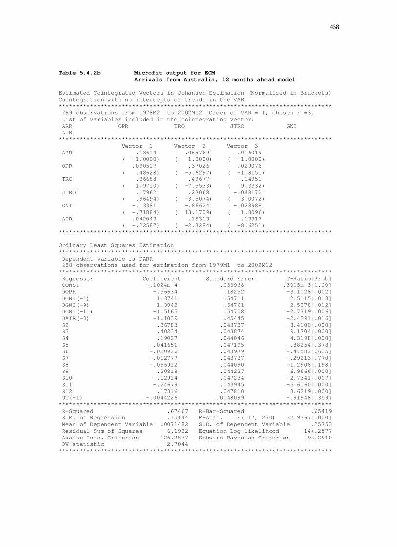
458

Table 5.4.2b Microfit output for ECM Arrivals from Australia, 12 months ahead model Estimated Cointegrated Vectors in Johansen Estimation (Normalized in Brackets) Cointegration with no intercepts or trends in the VAR ****************************************************************************** 299 observations from 1978M2 to 2002M12. Order of VAR = 1, chosen r =3. List of variables included in the cointegrating vector: ARR OPR TRO JTRO GNI AIR ****************************************************************************** Vector 1 Vector 2 Vector 3 ARR -.18614 .065769 .016019 ( -1.0000) ( -1.0000) ( -1.0000) OPR .090517 .37026 .029076 ( .48628) ( -5.6297) ( -1.8151) TRO .36688 .49677 -.14951 ( 1.9710) ( -7.5533) ( 9.3332) JTRO .17962 .23068 -.048172 ( .96494) ( -3.5074) ( 3.0072) GNI -.13381 -.86624 -.028988 ( -.71884) ( 13.1709) ( 1.8096) AIR -.042043 .15313 .13817 ( -.22587) ( -2.3284) ( -8.6251) ****************************************************************************** Ordinary Least Squares Estimation ****************************************************************************** Dependent variable is DARR 288 observations used for estimation from 1979M1 to 2002M12 ****************************************************************************** Regressor Coefficient Standard Error T-Ratio[Prob] CONST -.1024E-4 .033968 -.3015E-3[1.00] DOPR -.56634 .18252 -3.1028[.002] DGNI(-4) 1.3741 .54711 2.5115[.013] DGNI(-9) 1.3842 .54761 2.5278[.012] DGNI(-11) -1.5165 .54708 -2.7719[.006] DAIR(-3) -1.1039 .45445 -2.4291[.016] S2 -.36783 .043737 -8.4100[.000] S3 .40234 .043874 9.1704[.000] S4 .19027 .044046 4.3198[.000] S5 -.041651 .047195 -.88254[.378] S6 -.020926 .043979 -.47582[.635] S7 -.012777 .043737 -.29213[.770] S8 -.056912 .044090 -1.2908[.198] S9 .30818 .044237 6.9666[.000] S10 -.12914 .047234 -2.7341[.007] S11 -.24679 .043945 -5.6160[.000] S12 .17316 .047810 3.6219[.000] UT(-1) -.0044226 .0048099 -.91948[.359] ****************************************************************************** R-Squared .67467 R-Bar-Squared .65419 S.E. of Regression .15144 F-stat. F( 17, 270) 32.9367[.000] Mean of Dependent Variable .0071482 S.D. of Dependent Variable .25753 Residual Sum of Squares 6.1922 Equation Log-likelihood 144.2577 Akaike Info. Criterion 126.2577 Schwarz Bayesian Criterion 93.2910 DW-statistic 2.7044 ******************************************************************************

459

Table 5.4.2c Microfit output for ECM Arrivals from Australia, 24 months ahead model Estimated Cointegrated Vectors in Johansen Estimation (Normalized in Brackets) Cointegration with no intercepts or trends in the VAR ****************************************************************************** 287 observations from 1978M2 to 2001M12. Order of VAR = 1, chosen r =3. List of variables included in the cointegrating vector: ARR OPR TRO JTRO GNI AIR ****************************************************************************** Vector 1 Vector 2 Vector 3 ARR -.19372 -.057234 .021415 ( -1.0000) ( -1.0000) ( -1.0000) OPR .079376 -.36445 .061534 ( .40974) ( -6.3677) ( -2.8735) TRO .33556 -.54089 -.13274 ( 1.7322) ( -9.4506) ( 6.1984) JTRO .15813 -.26265 -.057475 ( .81625) ( -4.5891) ( 2.6839) GNI -.079619 .88681 -.068336 ( -.41099) ( 15.4945) ( 3.1911) AIR -.048814 -.13774 .14979 ( -.25198) ( -2.4067) ( -6.9947) ****************************************************************************** Ordinary Least Squares Estimation ****************************************************************************** Dependent variable is DARR 276 observations used for estimation from 1979M1 to 2001M12 ****************************************************************************** Regressor Coefficient Standard Error T-Ratio[Prob] CONST .0054227 .034863 .15554[.877] DOPR -.57480 .18762 -3.0636[.002] DGNI(-4) 1.4878 .56393 2.6382[.009] DGNI(-9) 1.3862 .56418 2.4571[.015] DGNI(-11) -1.4004 .56378 -2.4839[.014] DAIR(-3) -1.0915 .45978 -2.3740[.018] S2 -.37352 .045260 -8.2527[.000] S3 .40364 .045462 8.8786[.000] S4 .19184 .045548 4.2119[.000] S5 -.054425 .049216 -1.1059[.270] S6 -.026881 .045497 -.59082[.555] S7 -.021269 .045260 -.46994[.639] S8 -.057260 .045622 -1.2551[.211] S9 .30640 .045865 6.6806[.000] S10 -.13045 .049290 -2.6466[.009] S11 -.25222 .045459 -5.5483[.000] S12 .15949 .049945 3.1933[.002] UT(-1) -.0072919 .0063451 -1.1492[.252] ****************************************************************************** R-Squared .67308 R-Bar-Squared .65154 S.E. of Regression .15340 F-stat. F( 17, 258) 31.2463[.000] Mean of Dependent Variable .0074300 S.D. of Dependent Variable .25986 Residual Sum of Squares 6.0708 Equation Log-likelihood 135.1066 Akaike Info. Criterion 117.1066 Schwarz Bayesian Criterion 84.5230 DW-statistic 2.7053 ******************************************************************************

460

Table 5.4.3a Microfit output for ECM Arrivals from Canada, one month ahead model Estimated Cointegrated Vectors in Johansen Estimation (Normalized in Brackets) Cointegration with no intercepts or trends in the VAR ****************************************************************************** 288 observations from 1978M2 to 2002M1 . Order of VAR = 1, chosen r =3. List of variables included in the cointegrating vector: ARR OPR TRO JTRO GNI AIR ****************************************************************************** Vector 1 Vector 2 Vector 3 ARR .33774 .055851 -.0027564 ( -1.0000) ( -1.0000) ( -1.0000) OPR .049296 -.047543 -.073901 ( -.14596) ( .85124) ( -26.8104) TRO -.35007 .75365 .026944 ( 1.0365) ( -13.4939) ( 9.7751) JTRO -.11974 -.23657 -.011813 ( .35453) ( 4.2357) ( -4.2855) GNI -.23389 .061156 -.031229 ( .69251) ( -1.0950) ( -11.3295) AIR .11735 -.53283 .038323 ( -.34747) ( 9.5402) ( 13.9032) ****************************************************************************** Ordinary Least Squares Estimation ****************************************************************************** Dependent variable is DARR 276 observations used for estimation from 1979M2 to 2002M1 ****************************************************************************** Regressor Coefficient Standard Error T-Ratio[Prob] CONST .12038 .025490 4.7229[.000] DOPR(-12) -.33537 .15713 -2.1344[.034] DTRO .44242 .16112 2.7459[.006] DJTRO(-5) .32761 .15057 2.1757[.030] DJTRO(-11) -.38353 .16122 -2.3789[.018] DGNI -1.3840 .46722 -2.9623[.003] DGNI(-7) -1.7645 .45001 -3.9210[.000] DGNI(-8) 1.1295 .46170 2.4464[.015] S2 -.36802 .031849 -11.5553[.000] S3 .065435 .032737 1.9988[.047] S4 -.083251 .033060 -2.5182[.012] S5 -.14078 .032506 -4.3308[.000] S6 -.32155 .032112 -10.0134[.000] S7 .041483 .031831 1.3032[.194] S8 -.12226 .036763 -3.3256[.001] S9 -.21411 .036473 -5.8705[.000] S10 .11072 .031571 3.5069[.001] S11 -.20449 .034721 -5.8896[.000] S12 -.20096 .032184 -6.2441[.000] UT(-1) -.51083 .051866 -9.8491[.000] ****************************************************************************** R-Squared .83494 R-Bar-Squared .82269 S.E. of Regression .091524 F-stat. F( 19, 256) 68.1537[.000] Mean of Dependent Variable .0052030 S.D. of Dependent Variable .21735 Residual Sum of Squares 2.1444 Equation Log-likelihood 278.7118 Akaike Info. Criterion 258.7118 Schwarz Bayesian Criterion 222.5078 DW-statistic 2.1430 ******************************************************************************

461

Table 5.4.3b Microfit output for ECM Arrivals from Canada, 12 months ahead model Estimated Cointegrated Vectors in Johansen Estimation (Normalized in Brackets) Cointegration with no intercepts or trends in the VAR ****************************************************************************** 299 observations from 1978M2 to 2002M12. Order of VAR = 1, chosen r =3. List of variables included in the cointegrating vector: ARR OPR TRO JTRO GNI AIR ****************************************************************************** Vector 1 Vector 2 Vector 3 ARR .33094 .054050 -.0014914 ( -1.0000) ( -1.0000) ( -1.0000) OPR .069717 -.046504 -.058987 ( -.21066) ( .86039) ( -39.5521) TRO -.33401 .75509 .030773 ( 1.0093) ( -13.9702) ( 20.6341) JTRO -.10852 -.23418 -.0037240 ( .32790) ( 4.3326) ( -2.4970) GNI -.23902 .060353 -.042285 ( .72224) ( -1.1166) ( -28.3530) AIR .10846 -.53220 .037471 ( -.32772) ( 9.8465) ( 25.1247) ****************************************************************************** Ordinary Least Squares Estimation ****************************************************************************** Dependent variable is DARR 291 observations used for estimation from 1978M10 to 2002M12 ****************************************************************************** Regressor Coefficient Standard Error T-Ratio[Prob] CONST .12805 .025816 4.9599[.000] DTRO .45801 .16331 2.8046[.005] DGNI -1.4818 .46240 -3.2045[.002] DGNI(-7) -1.8192 .45857 -3.9671[.000] DGNI(-8) 1.3066 .46889 2.7865[.006] S2 -.36559 .032248 -11.3371[.000] S3 .068892 .032615 2.1123[.036] S4 -.10701 .032970 -3.2458[.001] S5 -.14744 .032867 -4.4859[.000] S6 -.32245 .032223 -10.0068[.000] S7 .044036 .032083 1.3726[.171] S8 -.12890 .037071 -3.4772[.001] S9 -.24120 .036490 -6.6100[.000] S10 .10479 .031552 3.3212[.001] S11 -.20924 .034810 -6.0109[.000] S12 -.19938 .032058 -6.2193[.000] UT(-1) -.48070 .049112 -9.7878[.000] ****************************************************************************** R-Squared .82046 R-Bar-Squared .80997 S.E. of Regression .093729 F-stat. F( 16, 274) 78.2567[.000] Mean of Dependent Variable .0046053 S.D. of Dependent Variable .21501 Residual Sum of Squares 2.4071 Equation Log-likelihood 284.7468 Akaike Info. Criterion 267.7468 Schwarz Bayesian Criterion 236.5235 DW-statistic 2.1465 ******************************************************************************

462

Table 5.4.3c Microfit output for ECM Arrivals from Canada, 24 months ahead model Estimated Cointegrated Vectors in Johansen Estimation (Normalized in Brackets) Cointegration with no intercepts or trends in the VAR ****************************************************************************** 287 observations from 1978M2 to 2001M12. Order of VAR = 1, chosen r =3. List of variables included in the cointegrating vector: ARR OPR TRO JTRO GNI AIR ****************************************************************************** Vector 1 Vector 2 Vector 3 ARR .33801 .057337 -.0036617 ( -1.0000) ( -1.0000) ( -1.0000) OPR .042780 -.035093 -.096290 ( -.12656) ( .61206) ( -26.2963) TRO -.35560 .75518 .033435 ( 1.0520) ( -13.1709) ( 9.1309) JTRO -.12265 -.22996 -.028841 ( .36286) ( 4.0107) ( -7.8762) GNI -.23046 .052543 -.012427 ( .68181) ( -.91639) ( -3.3938) AIR .12057 -.53341 .029855 ( -.35672) ( 9.3030) ( 8.1534) ****************************************************************************** Ordinary Least Squares Estimation ****************************************************************************** Dependent variable is DARR 275 observations used for estimation from 1979M2 to 2001M12 ****************************************************************************** Regressor Coefficient Standard Error T-Ratio[Prob] CONST .11806 .026298 4.4895[.000] DOPR(-12) -.34228 .15780 -2.1690[.031] DTRO .44167 .16187 2.7286[.007] DJTRO(-5) .32718 .15134 2.1618[.032] DJTRO(-11) -.38825 .16196 -2.3972[.017] DGNI -1.3728 .47075 -2.9163[.004] DGNI(-7) -1.7727 .45210 -3.9209[.000] DGNI(-8) 1.1260 .46415 2.4260[.016] S2 -.36552 .032562 -11.2254[.000] S3 .068991 .033129 2.0825[.038] S4 -.080532 .033869 -2.3778[.018] S5 -.13845 .033284 -4.1598[.000] S6 -.31901 .032828 -9.7174[.000] S7 .045014 .032281 1.3944[.164] S8 -.11932 .037530 -3.1792[.002] S9 -.21095 .037191 -5.6721[.000] S10 .11369 .032168 3.5341[.000] S11 -.20281 .035627 -5.6925[.000] S12 -.19841 .032899 -6.0309[.000] UT(-1) -.50682 .052259 -9.6983[.000] ****************************************************************************** R-Squared .83407 R-Bar-Squared .82171 S.E. of Regression .091937 F-stat. F( 19, 255) 67.4639[.000] Mean of Dependent Variable .0050468 S.D. of Dependent Variable .21773 Residual Sum of Squares 2.1554 Equation Log-likelihood 276.5043 Akaike Info. Criterion 256.5043 Schwarz Bayesian Criterion 220.3366 DW-statistic 2.1313 ******************************************************************************

463

Table 5.4.4a Microfit output for ECM Arrivals from China, one month ahead model Estimated Cointegrated Vectors in Johansen Estimation (Normalized in Brackets) Cointegration with no intercepts or trends in the VAR ****************************************************************************** 288 observations from 1978M2 to 2002M1 . Order of VAR = 1, chosen r =3. List of variables included in the cointegrating vector: ARR OPR TRO GNI AIR ****************************************************************************** Vector 1 Vector 2 Vector 3 ARR -.17350 -.0031254 -.010104 ( -1.0000) ( -1.0000) ( -1.0000) OPR -.17761 -.17800 -.023547 ( -1.0237) ( -56.9540) ( -2.3304) TRO .0046900 -.038512 .013159 ( .027031) ( -12.3223) ( 1.3023) GNI .031801 -.17349 .083534 ( .18329) ( -55.5096) ( 8.2671) AIR .27461 .18784 -.029325 ( 1.5827) ( 60.1014) ( -2.9022) ****************************************************************************** Ordinary Least Squares Estimation ****************************************************************************** Dependent variable is DARR 277 observations used for estimation from 1979M1 to 2002M1 ****************************************************************************** Regressor Coefficient Standard Error T-Ratio[Prob] CONST .29412 .036466 8.0656[.000] DGNI(-11) 1.2287 .51594 2.3815[.018] S2 -.50501 .040924 -12.3402[.000] S3 .015701 .041032 .38265[.702] S4 -.20012 .040902 -4.8925[.000] S5 -.25318 .040815 -6.2031[.000] S6 -.42132 .040814 -10.3229[.000] S7 -.20771 .040833 -5.0868[.000] S8 -.10452 .040804 -2.5615[.011] S9 -.21410 .040794 -5.2483[.000] S10 -.23068 .040799 -5.6540[.000] S11 -.35617 .040820 -8.7253[.000] S12 -.68190 .053457 -12.7560[.000] UT(-1) -.0041337 .0039654 -1.0424[.298] ****************************************************************************** R-Squared .64035 R-Bar-Squared .62257 S.E. of Regression .13980 F-stat. F( 13, 263) 36.0204[.000] Mean of Dependent Variable .016134 S.D. of Dependent Variable .22756 Residual Sum of Squares 5.1401 Equation Log-likelihood 159.1455 Akaike Info. Criterion 145.1455 Schwarz Bayesian Criterion 119.7774 DW-statistic 2.5767 ******************************************************************************

464

Table 5.4.4b Microfit output for ECM Arrivals from China, 12 months ahead model Estimated Cointegrated Vectors in Johansen Estimation (Normalized in Brackets) Cointegration with no intercepts or trends in the VAR ****************************************************************************** 299 observations from 1978M2 to 2002M12. Order of VAR = 1, chosen r =3. List of variables included in the cointegrating vector: ARR OPR TRO GNI AIR ****************************************************************************** Vector 1 Vector 2 Vector 3 ARR -.17148 -.0037989 -.0056839 ( -1.0000) ( -1.0000) ( -1.0000) OPR -.17190 -.17707 -.012938 ( -1.0025) ( -46.6092) ( -2.2763) TRO .0062483 -.037938 .012498 ( .036438) ( -9.9865) ( 2.1987) GNI .014102 -.17711 .096463 ( .082237) ( -46.6215) ( 16.9711) AIR .27651 .18932 -.045164 ( 1.6125) ( 49.8354) ( -7.9458) ****************************************************************************** Ordinary Least Squares Estimation ****************************************************************************** Dependent variable is DARR 288 observations used for estimation from 1979M1 to 2002M12 ****************************************************************************** Regressor Coefficient Standard Error T-Ratio[Prob] CONST .28815 .037272 7.7310[.000] DGNI(-11) 1.2014 .52103 2.3058[.022] S2 -.49875 .041047 -12.1506[.000] S3 .013022 .041127 .31662[.752] S4 -.19789 .041006 -4.8258[.000] S5 -.26322 .040888 -6.4375[.000] S6 -.43177 .040889 -10.5595[.000] S7 -.19228 .040895 -4.7018[.000] S8 -.10669 .040853 -2.6115[.010] S9 -.21639 .040841 -5.2985[.000] S10 -.23369 .040824 -5.7244[.000] S11 -.36544 .040829 -8.9505[.000] S12 -.67518 .053710 -12.5709[.000] UT(-1) -.0017095 .0022777 -.75053[.454] ****************************************************************************** R-Squared .63196 R-Bar-Squared .61450 S.E. of Regression .14142 F-stat. F( 13, 274) 36.1913[.000] Mean of Dependent Variable .014519 S.D. of Dependent Variable .22777 Residual Sum of Squares 5.4796 Equation Log-likelihood 161.8621 Akaike Info. Criterion 147.8621 Schwarz Bayesian Criterion 122.2214 DW-statistic 2.5655 ******************************************************************************

465

Table 5.4.4c Microfit output for ECM Arrivals from China, 24 months ahead model Estimated Cointegrated Vectors in Johansen Estimation (Normalized in Brackets) Cointegration with no intercepts or trends in the VAR ****************************************************************************** 287 observations from 1978M2 to 2001M12. Order of VAR = 1, chosen r =2. List of variables included in the cointegrating vector: ARR OPR TRO GNI ****************************************************************************** Vector 1 Vector 2 ARR -.10203 -.026990 ( -1.0000) ( -1.0000) OPR .025762 -.066071 ( .25250) ( -2.4480) TRO .032179 .010980 ( .31539) ( .40684) GNI .20282 .11063 ( 1.9879) ( 4.0988) ****************************************************************************** Ordinary Least Squares Estimation ****************************************************************************** Dependent variable is DARR 276 observations used for estimation from 1979M1 to 2001M12 ****************************************************************************** Regressor Coefficient Standard Error T-Ratio[Prob] CONST .29761 .034228 8.6949[.000] DGNI(-11) 1.2768 .51365 2.4858[.014] S2 -.49773 .041056 -12.1233[.000] S3 .019688 .041207 .47777[.633] S4 -.19282 .041051 -4.6971[.000] S5 -.24400 .041042 -5.9451[.000] S6 -.41204 .041043 -10.0392[.000] S7 -.20090 .041041 -4.8951[.000] S8 -.096838 .041034 -2.3599[.019] S9 -.20412 .041074 -4.9695[.000] S10 -.22011 .041122 -5.3525[.000] S11 -.34473 .041192 -8.3688[.000] S12 -.67491 .053478 -12.6203[.000] UT(-1) -.017502 .0094867 -1.8449[.066] ****************************************************************************** R-Squared .64099 R-Bar-Squared .62318 S.E. of Regression .13915 F-stat. F( 13, 262) 35.9836[.000] Mean of Dependent Variable .014684 S.D. of Dependent Variable .22669 Residual Sum of Squares 5.0732 Equation Log-likelihood 159.8790 Akaike Info. Criterion 145.8790 Schwarz Bayesian Criterion 120.5362 DW-statistic 2.5770 ******************************************************************************

466

Table 5.4.5a Microfit output for ECM Arrivals from France, one month ahead model Estimated Cointegrated Vectors in Johansen Estimation (Normalized in Brackets) Cointegration with no intercepts or trends in the VAR ****************************************************************************** 287 observations from 1978M3 to 2002M1 . Order of VAR = 2, chosen r =2. List of variables included in the cointegrating vector: ARR OPR TRO GNI ****************************************************************************** Vector 1 Vector 2 ARR -.29372 -.010795 ( -1.0000) ( -1.0000) OPR -.045211 .10592 ( -.15393) ( 9.8119) TRO .20605 .25887 ( .70151) ( 23.9800) GNI .18242 -.22672 ( .62107) ( -21.0017) ****************************************************************************** Ordinary Least Squares Estimation ****************************************************************************** Dependent variable is DARR 283 observations used for estimation from 1978M7 to 2002M1 ****************************************************************************** Regressor Coefficient Standard Error T-Ratio[Prob] CONST -.051453 .028703 -1.7926[.074] DGNI(-5) -.49074 .23367 -2.1001[.037] S2 -.12022 .033519 -3.5867[.000] S3 .21746 .033354 6.5199[.000] S4 .18609 .037304 4.9884[.000] S5 .11404 .040940 2.7855[.006] S6 -.12701 .041279 -3.0769[.002] S7 .18408 .034498 5.3360[.000] S8 .017845 .038778 .46018[.646] S9 .14810 .036918 4.0116[.000] S10 .34284 .039543 8.6700[.000] S11 .024944 .047495 .52518[.600] S12 -.34198 .040840 -8.3735[.000] UT(-1) -.48854 .051664 -9.4561[.000] ****************************************************************************** R-Squared .80610 R-Bar-Squared .79673 S.E. of Regression .11428 F-stat. F( 13, 269) 86.0252[.000] Mean of Dependent Variable .0048420 S.D. of Dependent Variable .25348 Residual Sum of Squares 3.5132 Equation Log-likelihood 219.4739 Akaike Info. Criterion 205.4739 Schwarz Bayesian Criterion 179.9557 DW-statistic 2.1987 ******************************************************************************

467

Table 5.4.5b Microfit output for ECM Arrivals from France, 12 months ahead model Estimated Cointegrated Vectors in Johansen Estimation (Normalized in Brackets) Cointegration with no intercepts or trends in the VAR ****************************************************************************** 298 observations from 1978M3 to 2002M12. Order of VAR = 2, chosen r =2. List of variables included in the cointegrating vector: ARR OPR TRO GNI ****************************************************************************** Vector 1 Vector 2 ARR -.28814 -.012931 ( -1.0000) ( -1.0000) OPR -.038675 .10632 ( -.13423) ( 8.2220) TRO .21579 .25751 ( .74893) ( 19.9150) GNI .16694 -.22339 ( .57938) ( -17.2756) ****************************************************************************** Ordinary Least Squares Estimation ****************************************************************************** Dependent variable is DARR 294 observations used for estimation from 1978M7 to 2002M12 ****************************************************************************** Regressor Coefficient Standard Error T-Ratio[Prob] CONST -.050639 .028930 -1.7504[.081] DGNI(-5) -.59197 .23517 -2.5172[.012] S2 -.11320 .033804 -3.3488[.001] S3 .21803 .033581 6.4926[.000] S4 .18826 .037448 5.0272[.000] S5 .10251 .040960 2.5027[.013] S6 -.11364 .040968 -2.7738[.006] S7 .18337 .034894 5.2551[.000] S8 .012859 .038873 .33080[.741] S9 .14353 .037005 3.8787[.000] S10 .33613 .039399 8.5315[.000] S11 .017440 .046835 .37236[.710] S12 -.33709 .040612 -8.3002[.000] UT(-1) -.47310 .049804 -9.4993[.000] ****************************************************************************** R-Squared .79438 R-Bar-Squared .78483 S.E. of Regression .11621 F-stat. F( 13, 280) 83.2111[.000] Mean of Dependent Variable .0042494 S.D. of Dependent Variable .25052 Residual Sum of Squares 3.7812 Equation Log-likelihood 222.8038 Akaike Info. Criterion 208.8038 Schwarz Bayesian Criterion 183.0187 DW-statistic 2.2095 ******************************************************************************

468

Table 5.4.5c Microfit output for ECM Arrivals from France, 24 months ahead model Estimated Cointegrated Vectors in Johansen Estimation (Normalized in Brackets) Cointegration with no intercepts or trends in the VAR ****************************************************************************** 286 observations from 1978M3 to 2001M12. Order of VAR = 2, chosen r =2. List of variables included in the cointegrating vector: ARR OPR TRO GNI ****************************************************************************** Vector 1 Vector 2 ARR -.29388 -.010987 ( -1.0000) ( -1.0000) OPR -.045789 .10625 ( -.15581) ( 9.6700) TRO .20424 .26106 ( .69499) ( 23.7603) GNI .18413 -.22828 ( .62656) ( -20.7769) ****************************************************************************** Ordinary Least Squares Estimation ****************************************************************************** Dependent variable is DARR 282 observations used for estimation from 1978M7 to 2001M12 ****************************************************************************** Regressor Coefficient Standard Error T-Ratio[Prob] CONST -.061400 .029681 -2.0687[.040] DGNI(-5) -.48721 .23336 -2.0878[.038] S2 -.11281 .033925 -3.3254[.001] S3 .22428 .033689 6.6576[.000] S4 .19654 .038066 5.1632[.000] S5 .12609 .041871 3.0114[.003] S6 -.11522 .042152 -2.7335[.007] S7 .19304 .035092 5.5010[.000] S8 .029134 .039638 .73500[.463] S9 .15856 .037685 4.2075[.000] S10 .35451 .040440 8.7662[.000] S11 .039440 .048658 .81056[.418] S12 -.32976 .041792 -7.8905[.000] UT(-1) -.50023 .052346 -9.5562[.000] ****************************************************************************** R-Squared .80731 R-Bar-Squared .79796 S.E. of Regression .11412 F-stat. F( 13, 268) 86.3692[.000] Mean of Dependent Variable .0045983 S.D. of Dependent Variable .25389 Residual Sum of Squares 3.4905 Equation Log-likelihood 219.1137 Akaike Info. Criterion 205.1137 Schwarz Bayesian Criterion 179.6204 DW-statistic 2.1736 ******************************************************************************

469

Table 5.4.6a Microfit output for ECM Arrivals from Germany, one month ahead model Estimated Cointegrated Vectors in Johansen Estimation (Normalized in Brackets) Cointegration with no intercepts or trends in the VAR ****************************************************************************** 288 observations from 1978M2 to 2002M1 . Order of VAR = 1, chosen r =3. List of variables included in the cointegrating vector: ARR OPR TRO GNI AIR ****************************************************************************** Vector 1 Vector 2 Vector 3 ARR -.20815 -.041008 .020014 ( -1.0000) ( -1.0000) ( -1.0000) OPR -.030475 .040025 .17743 ( -.14641) ( .97603) ( -8.8653) TRO .15491 .18634 .14366 ( .74424) ( 4.5440) ( -7.1778) GNI .11732 -.18211 -.17594 ( .56364) ( -4.4409) ( 8.7910) AIR -.0069730 .046896 -.022766 ( -.033500) ( 1.1436) ( 1.1375) ****************************************************************************** Ordinary Least Squares Estimation ****************************************************************************** Dependent variable is DARR 286 observations used for estimation from 1978M4 to 2002M1 ****************************************************************************** Regressor Coefficient Standard Error T-Ratio[Prob] CONST .0075045 .030995 .24212[.809] DOPR(-2) .19938 .10277 1.9401[.053] S2 -.12862 .031041 -4.1435[.000] S3 .31141 .031125 10.0052[.000] S4 .10933 .041412 2.6400[.009] S5 -.022697 .043685 -.51956[.604] S6 -.32375 .040410 -8.0118[.000] S7 .089396 .031637 2.8257[.005] S8 -.086688 .035764 -2.4239[.016] S9 .12049 .034424 3.5000[.001] S10 .34267 .039283 8.7230[.000] S11 -.095090 .050898 -1.8682[.063] S12 -.58568 .042274 -13.8542[.000] UT(-1) -.39112 .047293 -8.2703[.000] ****************************************************************************** R-Squared .89514 R-Bar-Squared .89013 S.E. of Regression .10317 F-stat. F( 13, 272) 178.6154[.000] Mean of Dependent Variable .0019746 S.D. of Dependent Variable .31125 Residual Sum of Squares 2.8950 Equation Log-likelihood 250.9815 Akaike Info. Criterion 236.9815 Schwarz Bayesian Criterion 211.3895 DW-statistic 2.2273 ******************************************************************************

470

Table 5.4.6b Microfit output for ECM Arrivals from Germany, 12 months ahead model Estimated Cointegrated Vectors in Johansen Estimation (Normalized in Brackets) Cointegration with no intercepts or trends in the VAR ****************************************************************************** 299 observations from 1978M2 to 2002M12. Order of VAR = 1, chosen r =4. List of variables included in the cointegrating vector: ARR OPR TRO GNI AIR ****************************************************************************** Vector 1 Vector 2 Vector 3 Vector 4 ARR -.20585 .036968 .018525 .0080093 ( -1.0000) ( -1.0000) ( -1.0000) ( -1.0000) OPR -.030447 -.039043 .17769 -.0089466 ( -.14791) ( 1.0561) ( -9.5918) ( 1.1170) TRO .16087 -.17619 .14259 -.27952 ( .78149) ( 4.7661) ( -7.6970) ( 34.8990) GNI .10504 .17427 -.17237 .25894 ( .51026) ( -4.7140) ( 9.3045) ( -32.3302) AIR -.0024530 -.043308 -.023968 -.013787 ( -.011917) ( 1.1715) ( 1.2938) ( 1.7214) ****************************************************************************** Ordinary Least Squares Estimation ****************************************************************************** Dependent variable is DARR 290 observations used for estimation from 1978M11 to 2002M12 ****************************************************************************** Regressor Coefficient Standard Error T-Ratio[Prob] CONST -.010816 .032210 -.33580[.737] DAIR(-9) -.30677 .13700 -2.2392[.026] S2 -.11675 .031888 -3.6613[.000] S3 .31959 .031912 10.0146[.000] S4 .13446 .043053 3.1231[.002] S5 -.0010701 .044956 -.023802[.981] S6 -.27202 .041600 -6.5390[.000] S7 .090949 .033107 2.7471[.006] S8 -.077903 .037199 -2.0942[.037] S9 .13120 .035502 3.6957[.000] S10 .36527 .040395 9.0424[.000] S11 -.053299 .052489 -1.0154[.311] S12 -.54411 .043626 -12.4722[.000] UT(-1) -.42908 .048984 -8.7596[.000] ****************************************************************************** R-Squared .88682 R-Bar-Squared .88149 S.E. of Regression .10668 F-stat. F( 13, 276) 166.3606[.000] Mean of Dependent Variable .0010631 S.D. of Dependent Variable .30990 Residual Sum of Squares 3.1412 Equation Log-likelihood 244.6746 Akaike Info. Criterion 230.6746 Schwarz Bayesian Criterion 204.9854 DW-statistic 2.2109 ******************************************************************************

471

Table 5.4.6c Microfit output for ECM Arrivals from Germany, 24 months ahead model Estimated Cointegrated Vectors in Johansen Estimation (Normalized in Brackets) Cointegration with no intercepts or trends in the VAR ****************************************************************************** 287 observations from 1978M2 to 2001M12. Order of VAR = 1, chosen r =3. List of variables included in the cointegrating vector: ARR OPR TRO GNI AIR ****************************************************************************** Vector 1 Vector 2 Vector 3 ARR -.20795 -.043026 .021016 ( -1.0000) ( -1.0000) ( -1.0000) OPR -.030945 .042183 .17700 ( -.14881) ( .98041) ( -8.4222) TRO .15358 .18646 .13986 ( .73855) ( 4.3337) ( -6.6552) GNI .11888 -.17852 -.17316 ( .57166) ( -4.1491) ( 8.2394) AIR -.0073754 .044791 -.023091 ( -.035467) ( 1.0410) ( 1.0988) ****************************************************************************** Ordinary Least Squares Estimation ****************************************************************************** Dependent variable is DARR 285 observations used for estimation from 1978M4 to 2001M12 ****************************************************************************** Regressor Coefficient Standard Error T-Ratio[Prob] CONST -.0031311 .031784 -.098513[.922] DOPR(-2) .20459 .10265 1.9931[.047] S2 -.12139 .031407 -3.8651[.000] S3 .31894 .031522 10.1180[.000] S4 .11957 .041997 2.8472[.005] S5 -.011941 .044295 -.26958[.788] S6 -.31373 .040982 -7.6554[.000] S7 .097283 .032074 3.0331[.003] S8 -.077566 .036294 -2.1371[.033] S9 .12924 .034927 3.7002[.000] S10 .35257 .039854 8.8467[.000] S11 -.083126 .051538 -1.6129[.108] S12 -.57516 .042872 -13.4155[.000] UT(-1) -.39755 .047422 -8.3834[.000] ****************************************************************************** R-Squared .89566 R-Bar-Squared .89066 S.E. of Regression .10299 F-stat. F( 13, 271) 178.9511[.000] Mean of Dependent Variable .0011336 S.D. of Dependent Variable .31147 Residual Sum of Squares 2.8746 Equation Log-likelihood 250.6123 Akaike Info. Criterion 236.6123 Schwarz Bayesian Criterion 211.0448 DW-statistic 2.2265 ******************************************************************************

472

Table 5.4.7a Microfit output for ECM Arrivals from Korea, one month ahead model Estimated Cointegrated Vectors in Johansen Estimation (Normalized in Brackets) Cointegration with no intercepts or trends in the VAR ****************************************************************************** 288 observations from 1978M2 to 2002M1 . Order of VAR = 1, chosen r =2. List of variables included in the cointegrating vector: ARR OPR TRO JTRO GNI AIR ****************************************************************************** Vector 1 Vector 2 ARR .20156 -.15965 ( -1.0000) ( -1.0000) OPR .12086 .060669 ( -.59960) ( .38002) TRO -.088474 .11520 ( .43895) ( .72158) JTRO -.19733 .021971 ( .97900) ( .13762) GNI -.26560 .15402 ( 1.3177) ( .96472) AIR .073886 -.016778 ( -.36657) ( -.10509) ****************************************************************************** Ordinary Least Squares Estimation ****************************************************************************** Dependent variable is DARR 277 observations used for estimation from 1979M1 to 2002M1 ****************************************************************************** Regressor Coefficient Standard Error T-Ratio[Prob] CONST .091663 .019720 4.6481[.000] DTRO -.18626 .088078 -2.1147[.035] DGNI .60376 .16137 3.7414[.000] DGNI(-8) .28097 .14230 1.9745[.049] DAIR(-11) -.076414 .035267 -2.1668[.031] S2 -.23773 .025301 -9.3958[.000] S3 .012159 .024828 .48971[.625] S4 -.058762 .024988 -2.3516[.019] S5 -.067387 .025189 -2.6752[.008] S6 -.15605 .025178 -6.1979[.000] S7 .085710 .024970 3.4326[.001] S8 .023960 .025823 .92786[.354] S9 -.33392 .029172 -11.4463[.000] S10 .037099 .025109 1.4775[.141] S11 -.10449 .025927 -4.0302[.000] S12 -.18960 .025729 -7.3690[.000] UT(-1) -.051455 .022134 -2.3246[.021] ****************************************************************************** R-Squared .75906 R-Bar-Squared .74423 S.E. of Regression .073691 F-stat. F( 16, 260) 51.1930[.000] Mean of Dependent Variable .0099610 S.D. of Dependent Variable .14571 Residual Sum of Squares 1.4119 Equation Log-likelihood 338.1058 Akaike Info. Criterion 321.1058 Schwarz Bayesian Criterion 290.3016 DW-statistic 2.2125 ******************************************************************************

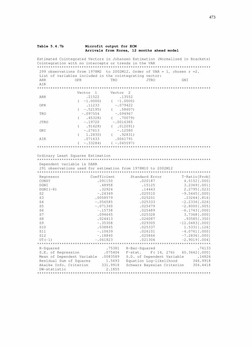
473

Table 5.4.7b Microfit output for ECM Arrivals from Korea, 12 months ahead model Estimated Cointegrated Vectors in Johansen Estimation (Normalized in Brackets) Cointegration with no intercepts or trends in the VAR ****************************************************************************** 299 observations from 1978M2 to 2002M12. Order of VAR = 1, chosen r =2. List of variables included in the cointegrating vector: ARR OPR TRO JTRO GNI AIR ****************************************************************************** Vector 1 Vector 2 ARR .21522 .13552 ( -1.0000) ( -1.0000) OPR .11233 -.079422 ( -.52195) ( .58607) TRO -.097554 -.094967 ( .45328) ( .70079) JTRO -.19720 -.0016385 ( .91628) ( .012091) GNI -.27613 -.12580 ( 1.2830) ( .92831) AIR .071633 .0061791 ( -.33284) ( -.045597) ****************************************************************************** Ordinary Least Squares Estimation ****************************************************************************** Dependent variable is DARR 291 observations used for estimation from 1978M10 to 2002M12 ****************************************************************************** Regressor Coefficient Standard Error T-Ratio[Prob] CONST .091150 .020187 4.5152[.000] DGNI .48958 .15125 3.2369[.001] DGNI(-8) .32924 .14443 2.2795[.023] S2 -.24349 .025510 -9.5445[.000] S3 .0058579 .025201 .23244[.816] S4 -.056585 .025333 -2.2336[.026] S5 -.071340 .025479 -2.8000[.005] S6 -.15738 .025489 -6.1743[.000] S7 .094645 .025328 3.7368[.000] S8 .024413 .026087 .93585[.350] S9 -.35308 .029305 -12.0483[.000] S10 .038845 .025337 1.5331[.126] S11 -.10639 .026101 -4.0761[.000] S12 -.18840 .025866 -7.2836[.000] UT(-1) -.061823 .021304 -2.9019[.004] ****************************************************************************** R-Squared .75381 R-Bar-Squared .74133 S.E. of Regression .075404 F-stat. F( 14, 276) 60.3642[.000] Mean of Dependent Variable .0083589 S.D. of Dependent Variable .14826 Residual Sum of Squares 1.5693 Equation Log-likelihood 346.9918 Akaike Info. Criterion 331.9918 Schwarz Bayesian Criterion 304.4418 DW-statistic 2.1855 ******************************************************************************

474

Table 5.4.7c Microfit output for ECM Arrivals from Korea, 24 months ahead model Estimated Cointegrated Vectors in Johansen Estimation (Normalized in Brackets) Cointegration with no intercepts or trends in the VAR ****************************************************************************** 287 observations from 1978M2 to 2001M12. Order of VAR = 1, chosen r =2. List of variables included in the cointegrating vector: ARR OPR TRO JTRO GNI AIR ****************************************************************************** Vector 1 Vector 2 ARR .20865 .15406 ( -1.0000) ( -1.0000) OPR .11760 -.071297 ( -.56361) ( .46278) TRO -.092397 -.10230 ( .44283) ( .66404) JTRO -.19839 -.017707 ( .95081) ( .11493) GNI -.27302 -.15095 ( 1.3085) ( .97982) AIR .074344 .012760 ( -.35631) ( -.082822) ****************************************************************************** Ordinary Least Squares Estimation ****************************************************************************** Dependent variable is DARR 276 observations used for estimation from 1979M1 to 2001M12 ****************************************************************************** Regressor Coefficient Standard Error T-Ratio[Prob] CONST .084651 .020161 4.1988[.000] DTRO -.20966 .087689 -2.3910[.018] DGNI .63502 .16147 3.9327[.000] DAIR(-9) .068791 .034985 1.9663[.050] DAIR(-11) -.075092 .035146 -2.1366[.034] S2 -.23144 .025612 -9.0366[.000] S3 .017811 .025110 .70933[.479] S4 -.052919 .025281 -2.0932[.037] S5 -.060997 .025495 -2.3925[.017] S6 -.15016 .025484 -5.8924[.000] S7 .085388 .025465 3.3531[.001] S8 .030849 .026152 1.1796[.239] S9 -.30179 .026889 -11.2235[.000] S10 .043433 .025414 1.7091[.089] S11 -.097575 .026254 -3.7165[.000] S12 -.18435 .026060 -7.0739[.000] UT(-1) -.053679 .022348 -2.4020[.017] ****************************************************************************** R-Squared .75968 R-Bar-Squared .74483 S.E. of Regression .073490 F-stat. F( 16, 259) 51.1692[.000] Mean of Dependent Variable .0092421 S.D. of Dependent Variable .14548 Residual Sum of Squares 1.3988 Equation Log-likelihood 337.6750 Akaike Info. Criterion 320.6750 Schwarz Bayesian Criterion 289.9016 DW-statistic 2.2175 ******************************************************************************

475

Table 5.4.8a Microfit output for ECM Arrivals from Singapore, one month ahead model Estimated Cointegrated Vectors in Johansen Estimation (Normalized in Brackets) Cointegration with no intercepts or trends in the VAR ****************************************************************************** 288 observations from 1978M2 to 2002M1 . Order of VAR = 1, chosen r =2. List of variables included in the cointegrating vector: ARR JTRO GNI AIR ****************************************************************************** Vector 1 Vector 2 ARR -.15484 -.017927 ( -1.0000) ( -1.0000) JTRO .099051 .21040 ( .63972) ( 11.7366) GNI .074505 .089131 ( .48118) ( 4.9719) AIR .051157 -.17630 ( .33039) ( -9.8344) ****************************************************************************** Ordinary Least Squares Estimation ****************************************************************************** Dependent variable is DARR 276 observations used for estimation from 1979M2 to 2002M1 ****************************************************************************** Regressor Coefficient Standard Error T-Ratio[Prob] CONST -.84433 .056761 -14.8753[.000] DGNI(-11) -1.4756 .49217 -2.9983[.003] DGNI(-12) 1.4114 .49215 2.8679[.004] S2 .97969 .068862 14.2269[.000] S3 1.0602 .068857 15.3968[.000] S4 1.1771 .068731 17.1258[.000] S5 .83759 .068748 12.1833[.000] S6 1.1911 .068735 17.3293[.000] S7 .084492 .068771 1.2286[.220] S8 .80355 .068733 11.6908[.000] S9 1.1054 .068744 16.0806[.000] S10 .95902 .068761 13.9472[.000] S11 .96240 .068748 13.9989[.000] S12 1.1050 .079195 13.9525[.000] UT(-1) -.0024109 .0045834 -.52601[.599] ****************************************************************************** R-Squared .78953 R-Bar-Squared .77824 S.E. of Regression .19119 F-stat. F( 14, 261) 69.9354[.000] Mean of Dependent Variable .0062739 S.D. of Dependent Variable .40601 Residual Sum of Squares 9.5410 Equation Log-likelihood 72.7161 Akaike Info. Criterion 57.7161 Schwarz Bayesian Criterion 30.5631 DW-statistic 2.8975 ******************************************************************************

476

Table 5.4.8b Microfit output for ECM Arrivals from Singapore, 12 months ahead model Estimated Cointegrated Vectors in Johansen Estimation (Normalized in Brackets) Cointegration with no intercepts or trends in the VAR ****************************************************************************** 299 observations from 1978M2 to 2002M12. Order of VAR = 1, chosen r =2. List of variables included in the cointegrating vector: ARR JTRO GNI AIR ****************************************************************************** Vector 1 Vector 2 ARR -.15220 -.018203 ( -1.0000) ( -1.0000) JTRO .10106 .21220 ( .66400) ( 11.6570) GNI .076551 .089539 ( .50295) ( 4.9188) AIR .045627 -.17724 ( .29977) ( -9.7365) ****************************************************************************** Ordinary Least Squares Estimation ****************************************************************************** Dependent variable is DARR 287 observations used for estimation from 1979M2 to 2002M12 ****************************************************************************** Regressor Coefficient Standard Error T-Ratio[Prob] CONST -.84424 .057405 -14.7067[.000] DGNI(-11) -1.4576 .48312 -3.0171[.003] DGNI(-12) 1.4112 .49797 2.8339[.005] S2 .99448 .069201 14.3710[.000] S3 1.0604 .069192 15.3252[.000] S4 1.1653 .069056 16.8746[.000] S5 .83532 .069066 12.0944[.000] S6 1.1748 .069056 17.0122[.000] S7 .10114 .069087 1.4639[.144] S8 .79844 .069061 11.5614[.000] S9 1.1049 .069074 15.9955[.000] S10 .96370 .069094 13.9476[.000] S11 .97650 .069078 14.1361[.000] S12 1.1023 .078174 14.1007[.000] UT(-1) -.0025124 .0046630 -.53880[.590] ****************************************************************************** R-Squared .77945 R-Bar-Squared .76810 S.E. of Regression .19346 F-stat. F( 14, 272) 68.6642[.000] Mean of Dependent Variable .010609 S.D. of Dependent Variable .40173 Residual Sum of Squares 10.1799 Equation Log-likelihood 71.9213 Akaike Info. Criterion 56.9213 Schwarz Bayesian Criterion 29.4752 DW-statistic 2.8754 ******************************************************************************

477

Table 5.4.8c Microfit output for ECM Arrivals from Singapore, 24 months ahead model Estimated Cointegrated Vectors in Johansen Estimation (Normalized in Brackets) Cointegration with no intercepts or trends in the VAR ****************************************************************************** 287 observations from 1978M2 to 2001M12. Order of VAR = 1, chosen r =2. List of variables included in the cointegrating vector: ARR JTRO GNI AIR ****************************************************************************** Vector 1 Vector 2 ARR -.15563 -.020025 ( -1.0000) ( -1.0000) JTRO .098351 .20681 ( .63195) ( 10.3275) GNI .075523 .089103 ( .48527) ( 4.4495) AIR .051548 -.17227 ( .33122) ( -8.6025) ****************************************************************************** Ordinary Least Squares Estimation ****************************************************************************** Dependent variable is DARR 275 observations used for estimation from 1979M2 to 2001M12 ****************************************************************************** Regressor Coefficient Standard Error T-Ratio[Prob] CONST -.82589 .063083 -13.0920[.000] DGNI(-11) -1.4753 .49263 -2.9946[.003] DGNI(-12) 1.2693 .54062 2.3478[.020] S2 .96178 .074113 12.9772[.000] S3 1.0423 .074103 14.0660[.000] S4 1.1596 .073953 15.6808[.000] S5 .82044 .073960 11.0930[.000] S6 1.1739 .073951 15.8742[.000] S7 .067543 .073985 .91293[.362] S8 .78604 .073959 10.6281[.000] S9 1.0878 .073974 14.7058[.000] S10 .94148 .073990 12.7244[.000] S11 .94494 .073973 12.7740[.000] S12 1.0876 .083787 12.9801[.000] UT(-1) -.0031996 .0052127 -.61381[.540] ****************************************************************************** R-Squared .78446 R-Bar-Squared .77285 S.E. of Regression .19138 F-stat. F( 14, 260) 67.5895[.000] Mean of Dependent Variable .010170 S.D. of Dependent Variable .40155 Residual Sum of Squares 9.5227 Equation Log-likelihood 72.2171 Akaike Info. Criterion 57.2171 Schwarz Bayesian Criterion 30.0913 DW-statistic 2.9009 ******************************************************************************

478

Table 5.4.9a Microfit output for ECM Arrivals from Taiwan, one month ahead model Estimated Cointegrated Vectors in Johansen Estimation (Normalized in Brackets) Cointegration with no intercepts or trends in the VAR ****************************************************************************** 287 observations from 1978M3 to 2002M1 . Order of VAR = 2, chosen r =3. List of variables included in the cointegrating vector: ARR CPITAI JTRO AIR ****************************************************************************** Vector 1 Vector 2 Vector 3 ARR -.27304 -.053080 .052080 ( -1.0000) ( -1.0000) ( -1.0000) CPITAI .62189 .25261 .096016 ( 2.2777) ( 4.7590) ( -1.8436) JTRO -.017924 .10589 -.12929 ( -.065646) ( 1.9949) ( 2.4826) AIR .021594 -.10169 -.059169 ( .079089) ( -1.9159) ( 1.1361) ****************************************************************************** Ordinary Least Squares Estimation ****************************************************************************** Dependent variable is DARR 277 observations used for estimation from 1979M1 to 2002M1 ****************************************************************************** Regressor Coefficient Standard Error T-Ratio[Prob] CONST -.0077217 .036625 -.21083[.833] DCPITAI 3.3665 1.1334 2.9704[.003] DJTRO(-1) .55430 .27046 2.0494[.041] DAIR(-4) .17536 .041246 4.2516[.000] DAIR(-10) .14714 .039708 3.7056[.000] DAIR(-11) -.11974 .033533 -3.5708[.000] S2 .33400 .050661 6.5929[.000] S3 -.12110 .050706 -2.3882[.018] S4 .21430 .050441 4.2485[.000] S5 -.14676 .050658 -2.8971[.004] S6 -.097342 .050477 -1.9284[.055] S7 .44477 .051960 8.5599[.000] S8 -.18390 .051510 -3.5701[.000] S9 -.29026 .051257 -5.6629[.000] S10 .13283 .050548 2.6277[.009] S11 -.24058 .051644 -4.6584[.000] S12 -.12449 .051218 -2.4306[.016] UT(-1) -.021019 .010137 -2.0735[.039] ****************************************************************************** R-Squared .66678 R-Bar-Squared .64491 S.E. of Regression .17026 F-stat. F( 17, 259) 30.4858[.000] Mean of Dependent Variable .0069363 S.D. of Dependent Variable .28572 Residual Sum of Squares 7.5081 Equation Log-likelihood 106.6662 Akaike Info. Criterion 88.6662 Schwarz Bayesian Criterion 56.0501 DW-statistic 2.7848 ******************************************************************************

479

Table 5.4.9b Microfit output for ECM Arrivals from Taiwan, 12 months ahead model Estimated Cointegrated Vectors in Johansen Estimation (Normalized in Brackets) Cointegration with no intercepts or trends in the VAR ****************************************************************************** 298 observations from 1978M3 to 2002M12. Order of VAR = 2, chosen r =3. List of variables included in the cointegrating vector: ARR CPITAI JTRO AIR ****************************************************************************** Vector 1 Vector 2 Vector 3 ARR -.27140 -.050521 .051052 ( -1.0000) ( -1.0000) ( -1.0000) CPITAI .62088 .24206 .098350 ( 2.2877) ( 4.7912) ( -1.9265) JTRO -.018477 .11009 -.12889 ( -.068082) ( 2.1791) ( 2.5246) AIR .020505 -.10138 -.059270 ( .075553) ( -2.0067) ( 1.1610) ****************************************************************************** Ordinary Least Squares Estimation ****************************************************************************** Dependent variable is DARR 288 observations used for estimation from 1979M1 to 2002M12 ****************************************************************************** Regressor Coefficient Standard Error T-Ratio[Prob] CONST .0013485 .035529 .037955[.970] DCPITAI 3.4372 1.0830 3.1739[.002] DJTRO(-1) .64249 .25832 2.4872[.013] DAIR(-4) .16464 .040090 4.1067[.000] DAIR(-5) -.11781 .040512 -2.9079[.004] DAIR(-10) .14236 .038506 3.6969[.000] DAIR(-11) -.18033 .038715 -4.6580[.000] S2 .32362 .048553 6.6652[.000] S3 -.12578 .048736 -2.5808[.010] S4 .21011 .048387 4.3424[.000] S5 -.15121 .048587 -3.1122[.002] S6 -.10307 .048450 -2.1273[.034] S7 .43998 .049815 8.8323[.000] S8 -.18166 .049281 -3.6862[.000] S9 -.29799 .049070 -6.0727[.000] S10 .13519 .048445 2.7906[.006] S11 -.24153 .049473 -4.8820[.000] S12 -.12721 .049130 -2.5893[.010] UT(-1) -.0098239 .0098676 -.99557[.320] ****************************************************************************** R-Squared .68334 R-Bar-Squared .66215 S.E. of Regression .16505 F-stat. F( 18, 269) 32.2493[.000] Mean of Dependent Variable .0066863 S.D. of Dependent Variable .28396 Residual Sum of Squares 7.3280 Equation Log-likelihood 120.0061 Akaike Info. Criterion 101.0061 Schwarz Bayesian Criterion 66.2079 DW-statistic 2.8014 ******************************************************************************

480

Table 5.4.9c Microfit output for ECM Arrivals from Taiwan, 24 months ahead model Estimated Cointegrated Vectors in Johansen Estimation (Normalized in Brackets) Cointegration with no intercepts or trends in the VAR ****************************************************************************** 286 observations from 1978M3 to 2001M12. Order of VAR = 2, chosen r =3. List of variables included in the cointegrating vector: ARR CPITAI JTRO AIR ****************************************************************************** Vector 1 Vector 2 Vector 3 ARR -.27366 -.052382 .052474 ( -1.0000) ( -1.0000) ( -1.0000) CPITAI .62449 .25220 .095659 ( 2.2820) ( 4.8147) ( -1.8230) JTRO -.017950 .10555 -.13119 ( -.065593) ( 2.0150) ( 2.5002) AIR .021095 -.10217 -.058666 ( .077084) ( -1.9504) ( 1.1180) ****************************************************************************** Ordinary Least Squares Estimation ****************************************************************************** Dependent variable is DARR 276 observations used for estimation from 1979M1 to 2001M12 ****************************************************************************** Regressor Coefficient Standard Error T-Ratio[Prob] CONST -.011070 .037456 -.29553[.768] DCPITAI 3.3768 1.1353 2.9745[.003] DJTRO(-1) .56202 .27137 2.0710[.039] DAIR(-4) .17503 .041324 4.2356[.000] DAIR(-10) .14760 .039792 3.7093[.000] DAIR(-11) -.11977 .033589 -3.5657[.000] S2 .33767 .051333 6.5780[.000] S3 -.11771 .051337 -2.2928[.023] S4 .21766 .051075 4.2616[.000] S5 -.14344 .051307 -2.7956[.006] S6 -.094090 .051085 -1.8418[.067] S7 .44842 .052648 8.5172[.000] S8 -.18074 .052132 -3.4669[.001] S9 -.28715 .051848 -5.5384[.000] S10 .13635 .051204 2.6629[.008] S11 -.23708 .052298 -4.5333[.000] S12 -.12089 .051872 -2.3305[.021] UT(-1) -.020449 .0099883 -2.0473[.042] ****************************************************************************** R-Squared .66687 R-Bar-Squared .64492 S.E. of Regression .17055 F-stat. F( 17, 258) 30.3807[.000] Mean of Dependent Variable .0066591 S.D. of Dependent Variable .28620 Residual Sum of Squares 7.5041 Equation Log-likelihood 105.8563 Akaike Info. Criterion 87.8563 Schwarz Bayesian Criterion 55.2727 DW-statistic 2.7883 ******************************************************************************

481

Table 5.4.10a Microfit output for ECM Arrivals from the UK, one month ahead model Estimated Cointegrated Vectors in Johansen Estimation (Normalized in Brackets) Cointegration with no intercepts or trends in the VAR ****************************************************************************** 288 observations from 1978M2 to 2002M1 . Order of VAR = 1, chosen r =3. List of variables included in the cointegrating vector: ARR OPR TRO JTRO GNI AIR ****************************************************************************** Vector 1 Vector 2 Vector 3 ARR -.23289 .034797 .031281 ( -1.0000) ( -1.0000) ( -1.0000) OPR -.0045970 -.029684 .19150 ( -.019739) ( .85306) ( -6.1217) TRO .18262 -.29361 .37529 ( .78414) ( 8.4377) ( -11.9973) JTRO .12146 -.18832 -.043197 ( .52155) ( 5.4120) ( 1.3809) GNI .12850 .37484 -.40541 ( .55178) ( -10.7721) ( 12.9601) AIR -.019686 -.088104 .022108 ( -.084528) ( 2.5319) ( -.70674) ****************************************************************************** Ordinary Least Squares Estimation ****************************************************************************** Dependent variable is DARR 282 observations used for estimation from 1978M8 to 2002M1 ****************************************************************************** Regressor Coefficient Standard Error T-Ratio[Prob] CONST -.038817 .035537 -1.0923[.276] DTRO(-1) .80650 .32471 2.4837[.014] DJTRO .73924 .27304 2.7075[.007] DGNI(-6) -.90818 .41568 -2.1848[.030] S2 .14311 .050699 2.8227[.005] S3 .017073 .050822 .33594[.737] S4 .059463 .050723 1.1723[.242] S5 -.14169 .051008 -2.7778[.006] S6 -.022903 .050534 -.45323[.651] S7 .31617 .057944 5.4565[.000] S8 .10703 .050840 2.1052[.036] S9 -.14211 .050935 -2.7899[.006] S10 .11802 .049958 2.3624[.019] S11 -.071547 .050220 -1.4247[.155] S12 .013664 .049929 .27367[.785] UT(-1) -.31823 .045052 -7.0636[.000] ****************************************************************************** R-Squared .47000 R-Bar-Squared .44011 S.E. of Regression .17275 F-stat. F( 15, 266) 15.7258[.000] Mean of Dependent Variable .0040341 S.D. of Dependent Variable .23087 Residual Sum of Squares 7.9378 Equation Log-likelihood 103.2672 Akaike Info. Criterion 87.2672 Schwarz Bayesian Criterion 58.1319 DW-statistic 2.5536 ******************************************************************************

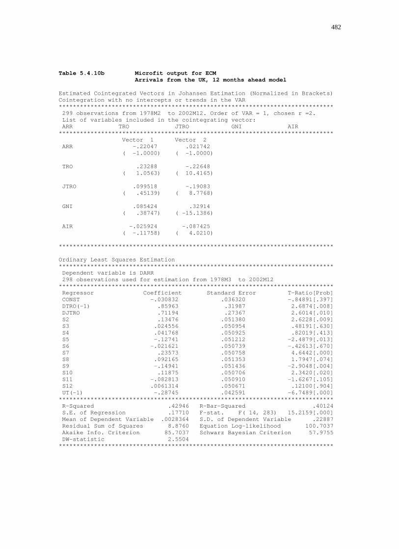
482

Table 5.4.10b Microfit output for ECM Arrivals from the UK, 12 months ahead model Estimated Cointegrated Vectors in Johansen Estimation (Normalized in Brackets) Cointegration with no intercepts or trends in the VAR ****************************************************************************** 299 observations from 1978M2 to 2002M12. Order of VAR = 1, chosen r =2. List of variables included in the cointegrating vector: ARR TRO JTRO GNI AIR ****************************************************************************** Vector 1 Vector 2 ARR -.22047 .021742 ( -1.0000) ( -1.0000) TRO .23288 -.22648 ( 1.0563) ( 10.4165) JTRO .099518 -.19083 ( .45139) ( 8.7768) GNI .085424 .32914 ( .38747) ( -15.1386) AIR -.025924 -.087425 ( -.11758) ( 4.0210) ****************************************************************************** Ordinary Least Squares Estimation ****************************************************************************** Dependent variable is DARR 298 observations used for estimation from 1978M3 to 2002M12 ****************************************************************************** Regressor Coefficient Standard Error T-Ratio[Prob] CONST -.030832 .036320 -.84891[.397] DTRO(-1) .85963 .31987 2.6874[.008] DJTRO .71194 .27367 2.6014[.010] S2 .13476 .051380 2.6228[.009] S3 .024556 .050954 .48191[.630] S4 .041768 .050925 .82019[.413] S5 -.12741 .051212 -2.4879[.013] S6 -.021621 .050739 -.42613[.670] S7 .23573 .050758 4.6442[.000] S8 .092165 .051353 1.7947[.074] S9 -.14941 .051436 -2.9048[.004] S10 .11875 .050706 2.3420[.020] S11 -.082813 .050910 -1.6267[.105] S12 .0061314 .050671 .12100[.904] UT(-1) -.28745 .042591 -6.7489[.000] ****************************************************************************** R-Squared .42946 R-Bar-Squared .40124 S.E. of Regression .17710 F-stat. F( 14, 283) 15.2159[.000] Mean of Dependent Variable .0028364 S.D. of Dependent Variable .22887 Residual Sum of Squares 8.8760 Equation Log-likelihood 100.7037 Akaike Info. Criterion 85.7037 Schwarz Bayesian Criterion 57.9755 DW-statistic 2.5504 ******************************************************************************

483

Table 5.4.10c Microfit output for ECM Arrivals from the UK, 24 months ahead model Estimated Cointegrated Vectors in Johansen Estimation (Normalized in Brackets) Cointegration with no intercepts or trends in the VAR ****************************************************************************** 287 observations from 1978M2 to 2001M12. Order of VAR = 1, chosen r =3. List of variables included in the cointegrating vector: ARR OPR TRO JTRO GNI AIR ****************************************************************************** Vector 1 Vector 2 Vector 3 ARR -.23713 .025947 .032129 ( -1.0000) ( -1.0000) ( -1.0000) OPR -.0077521 -.024069 .19807 ( -.032691) ( .92762) ( -6.1649) TRO .19167 -.27655 .37876 ( .80831) ( 10.6583) ( -11.7888) JTRO .12922 -.18529 -.034424 ( .54496) ( 7.1410) ( 1.0714) GNI .12198 .37057 -.42016 ( .51442) ( -14.2818) ( 13.0774) AIR -.017259 -.089088 .026393 ( -.072782) ( 3.4335) ( -.82146) ****************************************************************************** Ordinary Least Squares Estimation ****************************************************************************** Dependent variable is DARR 281 observations used for estimation from 1978M8 to 2001M12 ****************************************************************************** Regressor Coefficient Standard Error T-Ratio[Prob] CONST -.035203 .036278 -.97038[.333] DTRO(-1) .79292 .32664 2.4275[.016] DJTRO .75484 .27474 2.7474[.006] DGNI(-6) -.88855 .41603 -2.1358[.034] S2 .14109 .051455 2.7420[.007] S3 .015737 .051346 .30648[.759] S4 .057842 .051219 1.1293[.260] S5 -.14359 .051603 -2.7826[.006] S6 -.025508 .051223 -.49798[.619] S7 .31217 .058471 5.3389[.000] S8 .10539 .051380 2.0511[.041] S9 -.14348 .051386 -2.7922[.006] S10 .11571 .050578 2.2878[.023] S11 -.073481 .050759 -1.4476[.149] S12 .011083 .050590 .21908[.827] UT(-1) -.32266 .045833 -7.0400[.000] ****************************************************************************** R-Squared .47010 R-Bar-Squared .44010 S.E. of Regression .17296 F-stat. F( 15, 265) 15.6729[.000] Mean of Dependent Variable .0035679 S.D. of Dependent Variable .23114 Residual Sum of Squares 7.9272 Equation Log-likelihood 102.5897 Akaike Info. Criterion 86.5897 Schwarz Bayesian Criterion 57.4828 DW-statistic 2.5402 ******************************************************************************

484

Table 5.4.11a Microfit output for ECM Arrivals from the USA, one month ahead model Estimated Cointegrated Vectors in Johansen Estimation (Normalized in Brackets) Cointegration with no intercepts or trends in the VAR ****************************************************************************** 288 observations from 1978M2 to 2002M1 . Order of VAR = 1, chosen r =1. List of variables included in the cointegrating vector: ARR OPR TRO GNI AIR ****************************************************************************** Vector 1 ARR -.26631 ( -1.0000) OPR -.051441 ( -.19316) TRO .38927 ( 1.4617) GNI .22785 ( .85556) AIR -.051685 ( -.19407) ****************************************************************************** Ordinary Least Squares Estimation ****************************************************************************** Dependent variable is DARR 277 observations used for estimation from 1979M1 to 2002M1 ****************************************************************************** Regressor Coefficient Standard Error T-Ratio[Prob] CONST -.017359 .016919 -1.0260[.306] DGNI(-8) 1.6801 .37560 4.4733[.000] DGNI(-11) -1.3925 .37627 -3.7009[.000] S2 -.19490 .020224 -9.6370[.000] S3 .29803 .020934 14.2367[.000] S4 .089481 .021383 4.1847[.000] S5 .069248 .022617 3.0618[.002] S6 .017437 .023219 .75099[.453] S7 .019466 .022979 .84710[.398] S8 -.088846 .023027 -3.8583[.000] S9 -.046530 .028861 -1.6122[.108] S10 .25647 .021710 11.8137[.000] S11 -.19218 .026111 -7.3600[.000] S12 -.15701 .028973 -5.4192[.000] UT(-1) -.20602 .034306 -6.0054[.000] ****************************************************************************** R-Squared .87525 R-Bar-Squared .86858 S.E. of Regression .069285 F-stat. F( 14, 262) 131.2978[.000] Mean of Dependent Variable .0037159 S.D. of Dependent Variable .19112 Residual Sum of Squares 1.2577 Equation Log-likelihood 354.1234 Akaike Info. Criterion 339.1234 Schwarz Bayesian Criterion 311.9433 DW-statistic 1.9553 ******************************************************************************

485

Table 5.4.11b Microfit output for ECM Arrivals from the USA, 12 months ahead model Estimated Cointegrated Vectors in Johansen Estimation (Normalized in Brackets) Cointegration with no intercepts or trends in the VAR ****************************************************************************** 299 observations from 1978M2 to 2002M12. Order of VAR = 1, chosen r =2. List of variables included in the cointegrating vector: ARR OPR TRO GNI AIR ****************************************************************************** Vector 1 Vector 2 ARR -.26472 -.080699 ( -1.0000) ( -1.0000) OPR -.051329 -.11472 ( -.19390) ( -1.4216) TRO .38686 .0090065 ( 1.4614) ( .11161) GNI .22635 .12214 ( .85507) ( 1.5135) AIR -.051152 .013830 ( -.19323) ( .17138) ****************************************************************************** Ordinary Least Squares Estimation ****************************************************************************** Dependent variable is DARR 288 observations used for estimation from 1979M1 to 2002M12 ****************************************************************************** Regressor Coefficient Standard Error T-Ratio[Prob] CONST -.024392 .017029 -1.4324[.153] DTRO(-6) -.70540 .31948 -2.2080[.028] DGNI(-8) 1.7045 .37017 4.6047[.000] DGNI(-11) -1.4621 .37153 -3.9352[.000] S2 -.18251 .020312 -8.9850[.000] S3 .30955 .021039 14.7131[.000] S4 .091118 .021311 4.2757[.000] S5 .071224 .022377 3.1829[.002] S6 .028960 .023011 1.2585[.209] S7 .028833 .023018 1.2526[.211] S8 -.088105 .022798 -3.8646[.000] S9 -.036586 .028875 -1.2670[.206] S10 .26147 .021520 12.1503[.000] S11 -.17794 .026209 -6.7893[.000] S12 -.13989 .028262 -4.9498[.000] UT(-1) -.21355 .033758 -6.3259[.000] ****************************************************************************** R-Squared .87502 R-Bar-Squared .86813 S.E. of Regression .069150 F-stat. F( 15, 272) 126.9602[.000] Mean of Dependent Variable .0037654 S.D. of Dependent Variable .19042 Residual Sum of Squares 1.3006 Equation Log-likelihood 368.9601 Akaike Info. Criterion 352.9601 Schwarz Bayesian Criterion 323.6564 DW-statistic 1.9390 ******************************************************************************

486

Table 5.4.11c Microfit output for ECM Arrivals from the USA, 24 months ahead model Estimated Cointegrated Vectors in Johansen Estimation (Normalized in Brackets) Cointegration with no intercepts or trends in the VAR ****************************************************************************** 287 observations from 1978M2 to 2001M12. Order of VAR = 1, chosen r =1. List of variables included in the cointegrating vector: ARR OPR TRO GNI AIR ****************************************************************************** Vector 1 ARR -.26656 ( -1.0000) OPR -.049790 ( -.18679) TRO .39234 ( 1.4719) GNI .22558 ( .84627) AIR -.051121 ( -.19178) ****************************************************************************** Ordinary Least Squares Estimation ****************************************************************************** Dependent variable is DARR 276 observations used for estimation from 1979M1 to 2001M12 ****************************************************************************** Regressor Coefficient Standard Error T-Ratio[Prob] CONST -.016654 .017318 -.96167[.337] DGNI(-8) 1.6778 .37648 4.4567[.000] DGNI(-11) -1.3955 .37714 -3.7004[.000] S2 -.19503 .020482 -9.5224[.000] S3 .29812 .021134 14.1060[.000] S4 .089009 .021706 4.1007[.000] S5 .068622 .022955 2.9894[.003] S6 .016742 .023561 .71057[.478] S7 .018800 .023321 .80615[.421] S8 -.089492 .023371 -3.8292[.000] S9 -.046888 .029129 -1.6096[.109] S10 .25592 .022036 11.6138[.000] S11 -.19311 .026465 -7.2969[.000] S12 -.15741 .029245 -5.3825[.000] UT(-1) -.20454 .034371 -5.9511[.000] ****************************************************************************** R-Squared .87514 R-Bar-Squared .86844 S.E. of Regression .069449 F-stat. F( 14, 261) 130.6614[.000] Mean of Dependent Variable .0037114 S.D. of Dependent Variable .19147 Residual Sum of Squares 1.2588 Equation Log-likelihood 352.2209 Akaike Info. Criterion 337.2209 Schwarz Bayesian Criterion 310.0679 DW-statistic 1.9237 ******************************************************************************

cronus.uwindsor.cacronus.uwindsor.ca/units/isplab/isplab.nsf... · iii declaration “i, hubert...

Documents