˘ ˇˆ - gisresources.com˜ ˇˆ ˙ ˝ ˛ helén falkenström b 1321 stockholm, february 1999 r = -...

��

Helén FalkenströmB 1321

Stockholm, February 1999

R = - 0,831,50

1,70

1,90

2,10

2,30

2,50

2,70

0 10 20 30 40 50 60

Mean stand needle loss, %

Nor

mal

ised

rad

ianc

e va

lues

, NIR

ba

nd (

0,77

-0,8

6 µ

m)

Evaluation of IRS-1C LISS-3 satellite data for Norway spruce defoliation assessment IVL-rapport B1321

Organisation/OrganizationInstitutet för Vatten- och Luftvårdsforskning

RAPPORTSAMMANFATTNINGReport Summary

Adress/AddressBox 21060100 31 STOCKHOLM

Telefonnr/Telephone08-729 15 00

Projekttitel/Project title

Anslagsgivare för projektet/Projectsponsor

Rapportförfattare, author

Helén Falkenström

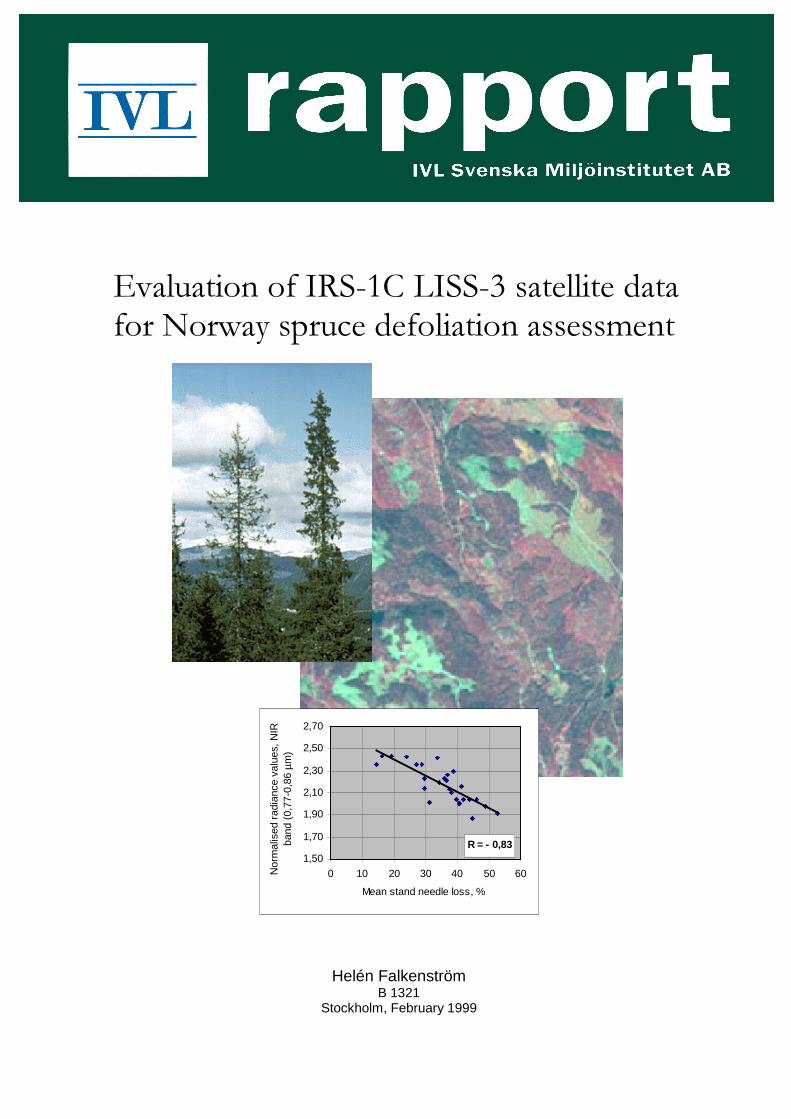
Rapportens titel och undertitel/Title and subtitle of the reportEvaluation of IRS-1C LISS-3 satellite data for Norway spruce defoliation assessment

Sammanfattning/SummarySatellite based remote sensing supported by air photo and field surveys, provide a means to areacovering forest health assessment on a regional scale. Landsat TM data has been extensively used instudies of spruce and fir defoliation in Europe and North America. The temporal coverage of LandsatTM in combination with cloudiness however restrict the availability of data. In this study the LISS-3sensor onboard the Indian Resource Satellite, IRS-1C, was evaluated for defoliation assessments inNorway spruce (Picea abies) in the central part of Sweden. The near infrared wavelength band provedto be best correlated with mean stand defoliation. After normalisation of satellite data for topographicconditions, the correlation coefficient increased from –0,19 to –0,83. Normalising satellite data forspecies composition did not improve the results though. The correction coefficients involved in theprocedure were originally developed for Landsat TM, and proved to be inadequate for the LISS-3 dataset. A thorough examination of the effects of species composition on LISS-3 data is needed to yieldbetter results. The correlation between observed defoliation in the verification stands and predicted(based on the inverse regression function between corrected NIR values and defoliation in referencestands) was 0,70, despite a very limited range of defoliation in the verification set. IRS-1C LISS-3 isfully comparable to Landsat TM for spruce defoliation studies, although the results would probably notbe significantly improved.

Nyckelord samt ev. anknytning till geografiskt område, näringsgren eller vattendrag/Keywords

Skogsvitalitet, fjärranalys, gran, IRS, LISS-3, Västernorrland

Bibliografiska uppgifter/Bibliographic data

IVL Rapport B 1321

Beställningsadress för rapporten/Ordering address

IVL, Publikationsservice, Box 21060, S-100 31 Stockholm, Sweden

Evaluation of IRS-1C LISS-3 satellite data for Norway spruce defoliation assessment. IVL-rapport B1321

Table of contents

Abstract.................................................................................................................................................... 41. Introduction......................................................................................................................................... 5

1.1. Objectives ..................................................................................................................................... 51.2. Satellite remote sensing and defoliation assessments ................................................................... 61.3. Factors influencing spectral effects of defoliation ........................................................................ 7

1.3.1. Atmospheric effects ............................................................................................................... 71.3.2. Forest stand parameters......................................................................................................... 71.3.3. Topography............................................................................................................................ 7

1.4. IRS LISS-3.................................................................................................................................. 102. Material and methods........................................................................................................................ 10

2.1. Study Area .................................................................................................................................. 102.2. Reference data............................................................................................................................. 12

2.2.1. Interpretation of aerial photographs ..................................................................................... 122.2.2. Field survey.......................................................................................................................... 12

2.3. Satellite data preprocessing......................................................................................................... 122.3.1. Geometric transformation .................................................................................................... 122.3.2. Conversion of digital numbers to physical units .................................................................. 122.3.3. Correction for atmospheric effects....................................................................................... 132.3.4. Extraction of radiance values .............................................................................................. 14

2.4. Normalisation of satellite data .................................................................................................... 142.4.1. Normalisation for topography.............................................................................................. 142.4.2. Normalisation for species composition ................................................................................ 15

2.5. Correlation between spruce defoliation and LISS-3 data............................................................ 152.6. Defoliation assessment algorithm and verification ..................................................................... 15

3. Results and discussion ...................................................................................................................... 163.1. Normalisation of satellite data .................................................................................................... 16

3.1.1. Normalisation for topography.............................................................................................. 163.1.2. Normalisation for species composition ................................................................................ 17

3.2. Correlation between spruce defoliation and LISS-3 data............................................................ 183.3. Defoliation assessment algorithm and verification ..................................................................... 193.4. IRS LISS-3 versus Landsat TM .................................................................................................. 203.5. Error sources ............................................................................................................................... 20

3.5.3. Correction for topography.................................................................................................... 213.5.4. Errors in reference data ........................................................................................................ 213.5.5. Radiometric correction......................................................................................................... 21

4. Conclusion ........................................................................................................................................ 22References.............................................................................................................................................. 23


4

Abstract

Satellite based remote sensing supported by air photo and field surveys, provide a means to areacovering forest health assessment on a regional scale. Landsat TM data has been extensively used instudies of spruce and fir defoliation in Europe and North America. The temporal coverage of LandsatTM in combination with cloudiness however restrict the availability of data. In this study the LISS-3sensor onboard the Indian Resource Satellite, IRS-1C, was evaluated for defoliation assessments inNorway spruce (Picea abies) in the central part of Sweden. The near infrared wavelength band provedto be best correlated with mean stand defoliation. After normalisation of satellite data for topographicconditions, the correlation coefficient increased from –0,19 to –0,83. Normalising satellite data forspecies composition did not improve the results though. The correction coefficients involved in theprocedure were originally developed for Landsat TM, and proved to be inadequate for the LISS-3 dataset. A thorough examination of the effects of species composition on LISS-3 data is needed to yieldbetter results. The correlation between observed defoliation in the verification stands and predicted(based on the inverse regression function between corrected NIR values and defoliation in referencestands) was 0,70, despite a very limited range of defoliation in the verification set. IRS-1C LISS-3 isfully comparable to Landsat TM for spruce defoliation studies, although the results would probably notbe significantly improved.


5

1. IntroductionThe issue of forest damage and decline attracted attention in the early 1980s when one of theeconomically most important coniferous species, Norway spruce (Picea abies), exhibited severedamage on a large scale in central Europe. In Sweden annual field surveys of forest defoliation anddiscoloration was initiated in 1984. Defoliation levels have proved to vary considerably betweendifferent years and geographic locations. Since the debate started the average percent of spruce trees inSweden with a severe defoliation have increased, although the levels have stabilised during the lastyears (Berghäll et al., 1995).

The debate on cause-effect mechanisms has been extensive. Reduced vitality is connected to bothnatural causes such as ageing, climatic stress and insect attacks, and human induced stress by airpollution and soil acidification associated with nutrient deficiencies (Hällgren, 1995; Nihlgård, 1996;Schulze, 1989). The importance of each factor is a matter of discussion. Recent research indicates thatthere is not one global explanation, but many, depending on each specific case. A widely supportedtheory stress that tree vitality seldom is attributed to one single cause, but a consequence of the conciseeffect of a combination of stress factors (Nihlgård, 1996). Nevertheless, irrespective of cause there is aneed for objective tools for area covering monitoring of short- and long-term changes in forest vitality.

Spaceborne techniques provide a means to assess defoliation on a regional scale and obtain areacovering output instead of statistically based. Whereas defoliation in field surveys and aerialphotography interpretation is estimated on single trees, assessments using satellite data concern themean defoliation of a forest stand or a pixel. The spatial resolution of satellite data makes the radianceregistered by the sensor in each pixel to be an integrated spectral response from the canopy andbackground reflectance. Factors such as structure of the canopy, species composition and topographythus tend to affect the assessments and needs to be corrected for.

The Landsat Thematic Mapper sensor, TM, has a resolution of 30 m and has been extensively used forstudies of the earth in many disciplines. A problem, though, is the temporal coverage of the satellitedata in combination with the fact that acquisitions frequently are affected by clouds. The time betweentwo Landsat TM acquisitions is in Sweden 8 days. This means that during the vegetation season, end ofMay to the end of August, merely about ten acquisitions take place. Due to the mid latitude weathersystems finding cloud free data is difficult. However, several new remote sensing satellites are on theirway to be launched and with more satellites in orbit the possibility to encounter a cloud free scene fromthe time of ones interest will increase.

The Indian remote sensing satellite IRS-1C was launched in December 1995, and its twin satellite IRS-1D in September 1997. They carry a multispectral sensor, LISS-3 with a resolution of 23.5 m, apancromatic camera with a 5.8 m resolution and a wide field sensor having a resolution of 188 m. TheLISS-3 sensor is comparable with Landsat TM in both resolution and other technical aspects. If datafrom IRS LISS-3 could be used as an alternative to Landsat TM data, the chance of acquiring cloudfree data would improve considerably and the remote sensing technique gain more interest.

1.1. ObjectivesThe overall aim of this study is to evaluate the performance of IRS-1C LISS-3 for assessing defoliationin Norway spruce (Picea abies). This includes:

1. To examine the correlation between mean stand defoliation and IRS-1C LISS-3 data.

2. To determine which LISS-3 band or combination of bands best discriminate among defoliationclasses.

3. To compare the performance of IRS-1C LISS-3 and Landsat TM for defoliation studies


6

1.2. Satellite remote sensing and defoliation assessmentsThe possibility to use satellite-based remote sensing to assess defoliation has been thoroughlyinvestigated by a number of authors. The majority of the studies concern Norway spruce (Picea abies)and Landsat TM data in the near and middle infrared regions of the electromagnetic spectra (e.g.Ekstrand, 1993; Lambert et al., 1995; Vogelmann, 1990). To a certain extent data from SPOT HRV hasalso been considered (Brockhaus et al.1992).

Significant correlations have been found between spruce defoliation and spectral reflectance registeredby the satellite sensors. The near infrared band, NIR, is involved in all studies, but while some obtainedbest results with various kinds of band ratios (Häusler, 1991; Vogelmann and Rock, 1988; Vogelmann,1990), others found the NIR band alone to be best correlated with defoliation (Brockhaus et al., 1992;Ekstrand, 1994; Heikkilä, 1998).

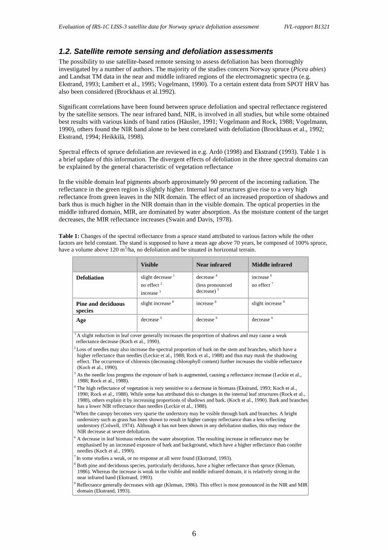
Spectral effects of spruce defoliation are reviewed in e.g. Ardö (1998) and Ekstrand (1993). Table 1 isa brief update of this information. The divergent effects of defoliation in the three spectral domains canbe explained by the general characteristic of vegetation reflectance

In the visible domain leaf pigments absorb approximately 90 percent of the incoming radiation. Thereflectance in the green region is slightly higher. Internal leaf structures give rise to a very highreflectance from green leaves in the NIR domain. The effect of an increased proportion of shadows andbark thus is much higher in the NIR domain than in the visible domain. The optical properties in themiddle infrared domain, MIR, are dominated by water absorption. As the moisture content of the targetdecreases, the MIR reflectance increases (Swain and Davis, 1978).

Table 1: Changes of the spectral reflectance from a spruce stand attributed to various factors while the otherfactors are held constant. The stand is supposed to have a mean age above 70 years, be composed of 100% spruce,have a volume above 120 m3/ha, no defoliation and be situated in horizontal terrain.

Visible Near infrared Middle infrared

Defoliation slight decrease 1

no effect 2

increase 3

decrease 4

(less pronounceddecrease) 5

increase 6

no effect 7

Pine and deciduousspecies

slight increase 8 increase 8 slight increase 8

Age decrease 9 decrease 9 decrease 9

1 A slight reduction in leaf cover generally increases the proportion of shadows and may cause a weakreflectance decrease (Koch et al., 1990).

2 Loss of needles may also increase the spectral proportion of bark on the stem and branches, which have ahigher reflectance than needles (Leckie et al., 1988; Rock et al., 1988) and thus may mask the shadowingeffect. The occurrence of chlorosis (decreasing chlorophyll content) further increases the visible reflectance(Koch et al., 1990).

3 As the needle loss progress the exposure of bark is augmented, causing a reflectance increase (Leckie et al.,1988; Rock et al., 1988).

4 The high reflectance of vegetation is very sensitive to a decrease in biomass (Ekstrand, 1993; Koch et al.,1990; Rock et al., 1988). While some has attributed this to changes in the internal leaf structures (Rock et al.,1988), others explain it by increasing proportions of shadows and bark. (Koch et al., 1990). Bark and brancheshas a lower NIR reflectance than needles (Leckie et al., 1988).

5 When the canopy becomes very sparse the understory may be visible through bark and branches. A brightunderstory such as grass has been shown to result in higher canopy reflectance than a less reflectingunderstory (Colwell, 1974). Although it has not been shown in any defoliation studies, this may reduce theNIR decrease at severe defoliation.

6 A decrease in leaf biomass reduces the water absorption. The resulting increase in reflectance may beemphasised by an increased exposure of bark and background, which have a higher reflectance than coniferneedles (Koch et al., 1990).

7 In some studies a weak, or no response at all were found (Ekstrand, 1993).8 Both pine and deciduous species, particularly deciduous, have a higher reflectance than spruce (Kleman,

1986). Whereas the increase is weak in the visible and middle infrared domain, it is relatively strong in thenear infrared band (Ekstrand, 1993).

9 Reflectance generally decreases with age (Kleman, 1986). This effect is most pronounced in the NIR and MIRdomain (Ekstrand, 1993).


7

1.3. Factors influencing spectral effects of defoliationThe spectral response of light and moderate defoliation is subtle and the capability to detect defoliationusing satellite and airborne data has proved to be very sensitive to atmospheric effects, variations inforest stand characteristics and terrain (e.g. Ekstrand, 1993; Leckie, 1987). In order to study defoliationthese factors thus need to be addressed.

1.3.1. Atmospheric effectsScattering and absorption by molecules and aerosols in the atmosphere affect all spaceborne data andthere are different ways to handle the problem. Absolute correction requires data on physical andmeteorological parameters as well as background reflectance values. The atmospheric effects arederived using a radiance transfer model (e.g. Kawata et al., 1988). Indirect corrections are based onassumed or field measured radiance from certain ground targets. By subtracting the radiance observedby the sensor with the known radiance, the path radiance is deduced. This approach neglects theatmospheric absorption and simply corrects for path radiance (Chavez, 1988).

A widely used indirect approach is dark object subtraction. Dark objects such as shadows and lakes areassumed to be completely, or nearly completely, black surfaces. Hence, the radiance registered at thesetargets is assumed to be an effect of path radiance. By subtracting the whole image with the radianceregistered at the dark targets, the path radiance is considered eliminated. Each band needs subtractionwith specific values since the scattering is wavelength dependent (Chavez, 1988). This approachassumes a horizontally uniform atmosphere, which is rarely the case. The aerosol and water content canvary significantly in space (Kaufman and Tanré, 1996). However, spatial information of theseparameters is in most cases not available. In this study a dark object subtraction was applied sinceneither meteorological data nor background reflectance values were available.

1.3.2. Forest stand parametersReflectance values in both the visible, near- and middle infrared parts of the spectrum generallydecrease with age, biomass, canopy closure, leaf area index and forest stand volume. These factors areusually positively correlated to each other. As the canopy closure reaches 100 percent the negativerelation with reflectance ceases. Volume continues to increase with age but no further decrease inreflectance will occur due to the sensitivity of the remotely sensed signal to canopy closure (Franklin,1986). The main reflectance change occurring with age (Table 1) is in fact caused by changes incanopy structure associated with age (and management practices) (Ekstrand, 1993).

Species composition has a large influence on the forest stand reflectance and the ability to assessdefoliation (Ekstrand, 1994; Leckie, 1987; Wastenson et al., 1987). Ekstrand (1994) found that acomponent of 25 percent pine completely neutralises the spectral effect of a 10 percent needle loss.Similarly is the spectral effect from a deciduous component of 20 percent in the same magnitude as a20 percent needle loss.

No standardised method to account for the effects of forest stand variations exists. In someinvestigation areas with homogeneous, monocultural and dense forest, it has not been considerednecessary. In other studies, only areas with similar forest conditions have been selected for the study.Ekstrand (1994) studied the effect of pine and deciduous trees in Swedish spruce forest. Subtractionconstants were empirically derived and multiplied with the percent of pine and deciduous content. Theresulting value was then subtracted from the original satellite number. This approach was tested in thepresent study.

1.3.3. TopographyTopography affects the sensor-registered radiance in several ways. The irradiance received by thetarget varies with the cosine of the angle between the sunbeam and the surface normal, i.e. theincidence angle (Figure 1). The larger the incidence angle, the less the amount of radiation reaching thesurface (Teillet et al., 1982). As the target receives less electromagnetic radiance, less electro-magneticradiance is reflected, if all other factors are constant.


8

Figure 1: The incidence angle, � is the angle between the sunbeam and the surfacenormal. A larger incidence angle means that less radiation reaches the surface.

Due to atmospheric scattering, the radiance received by the sensor is affected by the sun elevation aswell. A lower sun elevation means a longer transportation for the sunbeam, and the effect of scatteringis hence larger (Ekstrand, 1993). To some extent the target altitude also have an effect on the sensor-registered radiance). This is because the optical thickness of the atmosphere decreases with altitude andthe optical thickness affects the scattering (Yugui, 1989).

The amount of radiance reflected by the target depends on the class-specific reflection in differentdirections. But the class-specific reflection may change with topography if the geometric structurewithin the class, e.g. a forest canopy, change (e.g. Kriebel, 1976). Different types of vegetation responddifferently to direction and illumination effects (e.g. Thomson and Jones, 1990). A pine forest does forexample not respond in the same way as a spruce forest. The relative importance of slope-aspect effectsin forest reflectance is in fact not very well understood.

Several topographic correction models have been developed to remove the effects caused by terrainvariations. However, so far no correction procedure has been published that is valid and adequate forall vegetation types. Three common methods are the Lambert cosine correction, the Minnaertcorrection and the C-correction (further described below). To work with band ratios instead of singlebands, and in this way avoid the terrain effects, is another approach. It has been reported to be effectiveprovided that the atmospheric path term is eliminated (Kowalik et al., 1983). Still another way toaddress the problem is to correct for the effects of topography together with the atmospheric effects in aradiance transfer model (e.g. Kawata et al., 1988).

Lambert cosine correction: The Lambert cosine correction (Equation 1) assumes the target is aperfect diffuse reflector, i.e. that the reflectance is independent of viewing geometry. Hence, it onlyattempts to correct for illumination differences caused by surface orientation (Teillet et al., 1982). Butvery few surfaces are perfect diffuse reflectors (e.g. Lillesand and Kiefer, 1994).

Equation 1 (Teillet et al., 1982)

Equation 2 (Smith et al., 1980)

�� corr�� uncorr · cos (z) / cos (i)

cos i = cos (e) · cos (z) + sin (e) · sin (z) · cos ( s – n)

�� uncorr = spectral radiance measured by sensor (mWcm-2sr-1µm-1)�� corr = spectral radiance corrected for topography (mWcm-2sr-1µm-1)i = incidence angle, the angle between surface normal and solar beam (º)z = solar zenith angle (º)e = slope of reference site (º)

s = solar azimuth angle (º)n = slope aspect of reference site (º)s - n = ‘relative azimuth’ (º)

1�� 2 �� 3


9

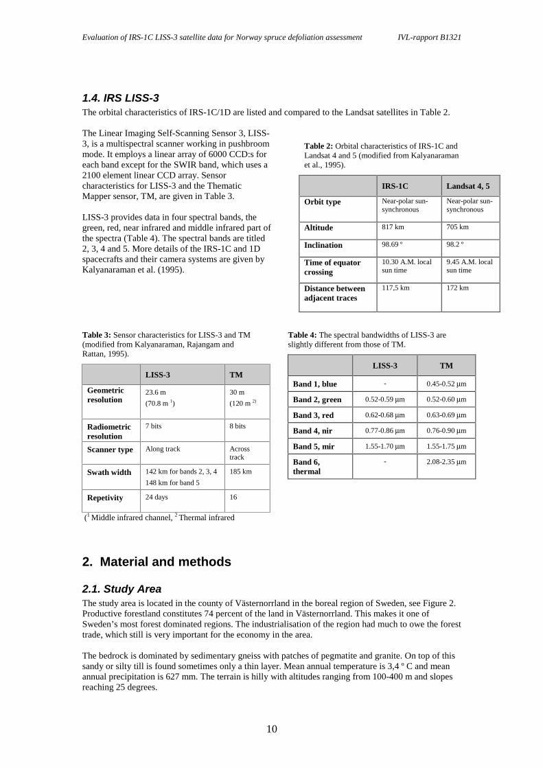
When sun elevation is low and northern slopes are in shadow no radiance would occur according to theLambertian assumption. This is not true since diffuse sky irradiance will always reach the surfaceduring daytime. According to Deering et al. (1994) sky irradiance may contribute to up to 15 percent ofthe total near infrared irradiance, and in the visible bands to as much as 25 percent.

The cosine correction usually underestimates reflectance on sun-facing slopes and overestimatereflectance on slopes facing away from the sun. Except for situations with high sun elevations, thecosine correction has proved to be inadequate for forest vegetation (e.g. Teillet et al., 1982; Smith etal., 1980).

Minnaert correction: The Minnnaert correction (Equation 3) is a variation of the cosine correctionand is based on the Minnaert law (Minnaert, 1941). A constant k, which is no real constant since it iswavelength and surface dependent, is introduced to simulate the non-Lambertian behaviour of the earthsurface. The Minnaert constant is a measure of how close a surface is to the ideal reflector, for whichk=1 (Smith et al., 1980).

Equation 3 (Smith et al., 1980)

C-correction: Teillet et al. (1982) examined a modified version of the cosine correction where a linearrelation between radiance and cosine of the incidence angle is still assumed. To avoid over correctionthey introduced a band specific constant derived from regression functions between radiance andcosine of the incidence angle. The constant is called C and is calculated by dividing the offset of theregression line with its slope.

Equation 4 (Teillet et al., 1982)

Meyer et al. (1993) tested the three correction models described above on TM forest images. TheMinnaert and c-correction both produced better results than the cosine correction. Best result wasachieved with the c-correction, but some degree of over- and underestimation remained also after the c-corrrection.

Ekstrand (1996) found a non-linear relation between radiance and cosine of the incidence angle whenstudying terrain effects on spruce forests in Sweden. He tested the Minnaert correction with previouslydeveloped constants, but the method was ineffective when a single constant for each spectral band wasused. When new constants were derived, however, and they were allowed to vary with the cosine of theincidence angle, the corrections proved adequate. For the near infrared channel residuals of 0,02mWcm-2sr-1µm-1 remained after correction.

The residual effects that remains after correction have generally been attributed to a neglecting of thediffusive illumination and poor digital terrain models (Civco, 1989). However, as pointed out byEkstrand (1993), there are gaps in the information about e.g. the diffuse sky irradiance, the classspecific reflection in different directions and changes in geometric canopy structure.

In this study the semi-empirical approach developed by Ekstrand (1996) for spruce forest and LandsatTM data was applied.

�� corr�� uncorr · cos (e) / [(cosk (i) · cosk (e)]

k = Minnaert constant

�� corr�� uncorr · [cos (z) + C] / [cos (i) + C]

C= a/m

C = C-constanta = offset of regression lineb = slope of regression line


10

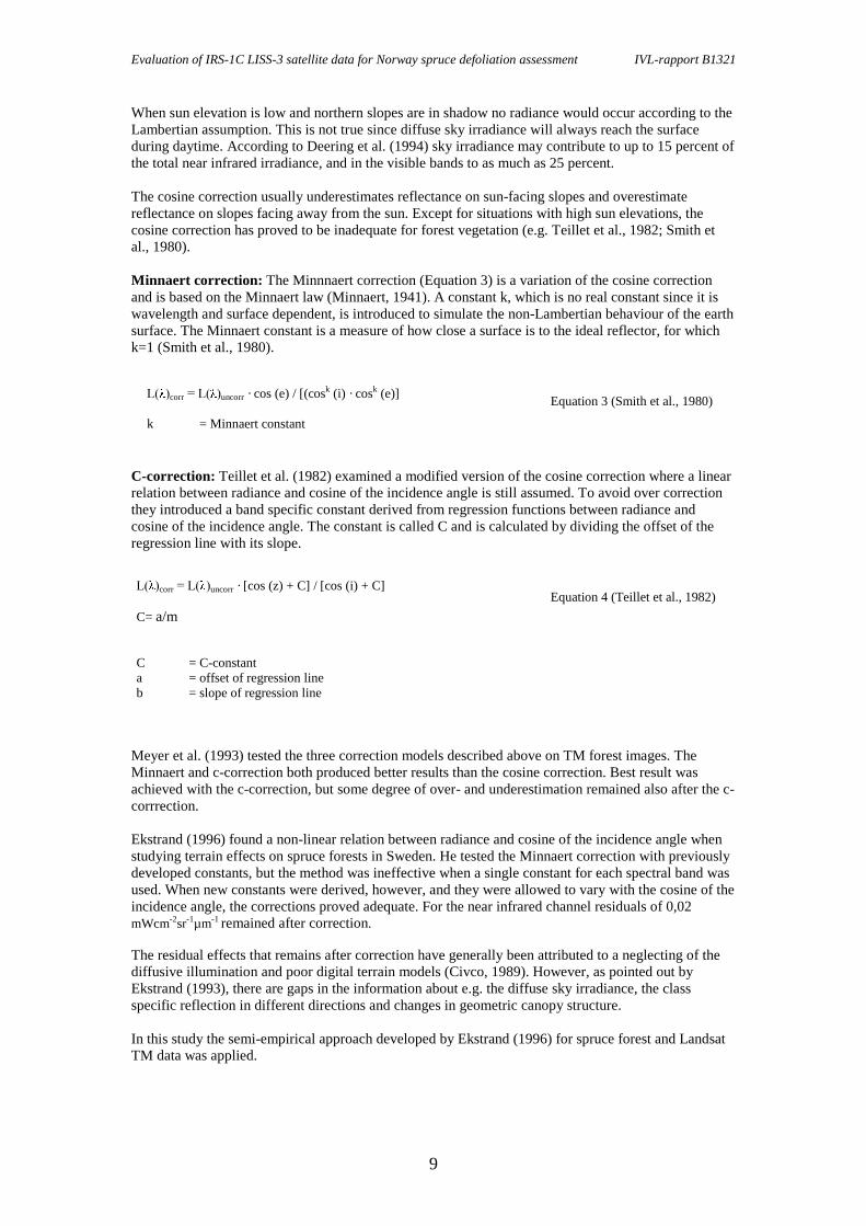
1.4. IRS LISS-3The orbital characteristics of IRS-1C/1D are listed and compared to the Landsat satellites in Table 2.

The Linear Imaging Self-Scanning Sensor 3, LISS-3, is a multispectral scanner working in pushbroommode. It employs a linear array of 6000 CCD:s foreach band except for the SWIR band, which uses a2100 element linear CCD array. Sensorcharacteristics for LISS-3 and the ThematicMapper sensor, TM, are given in Table 3.

LISS-3 provides data in four spectral bands, thegreen, red, near infrared and middle infrared part ofthe spectra (Table 4). The spectral bands are titled2, 3, 4 and 5. More details of the IRS-1C and 1Dspacecrafts and their camera systems are given byKalyanaraman et al. (1995).

Table 2: Orbital characteristics of IRS-1C andLandsat 4 and 5 (modified from Kalyanaramanet al., 1995).

IRS-1C Landsat 4, 5

Orbit type Near-polar sun-synchronous

Near-polar sun-synchronous

Altitude 817 km 705 km

Inclination 98.69 º 98.2 º

Time of equatorcrossing

10.30 A.M. localsun time

9.45 A.M. localsun time

Distance betweenadjacent traces

117,5 km 172 km

Table 3: Sensor characteristics for LISS-3 and TM(modified from Kalyanaraman, Rajangam andRattan, 1995).

LISS-3 TM

Geometricresolution

23.6 m

(70.8 m 1)

30 m

(120 m 2)

Radiometricresolution

7 bits 8 bits

Scanner type Along track Acrosstrack

Swath width 142 km for bands 2, 3, 4

148 km for band 5

185 km

Repetivity 24 days 16

(1 Middle infrared channel, 2 Thermal infrared

Table 4: The spectral bandwidths of LISS-3 areslightly different from those of TM.

LISS-3 TM

Band 1, blue - 0.45-0.52 µm

Band 2, green 0.52-0.59 µm 0.52-0.60 µm

Band 3, red 0.62-0.68 µm 0.63-0.69 µm

Band 4, nir 0.77-0.86 µm 0.76-0.90 µm

Band 5, mir 1.55-1.70 µm 1.55-1.75 µm

Band 6,thermal

- 2.08-2.35 µm

2. Material and methods

2.1. Study AreaThe study area is located in the county of Västernorrland in the boreal region of Sweden, see Figure 2.Productive forestland constitutes 74 percent of the land in Västernorrland. This makes it one ofSweden’s most forest dominated regions. The industrialisation of the region had much to owe the foresttrade, which still is very important for the economy in the area.

The bedrock is dominated by sedimentary gneiss with patches of pegmatite and granite. On top of thissandy or silty till is found sometimes only a thin layer. Mean annual temperature is 3,4 º C and meanannual precipitation is 627 mm. The terrain is hilly with altitudes ranging from 100-400 m and slopesreaching 25 degrees.


11

Figure 2: Location of study area.

Norway spruce (Picea abies) is the major species of the forest stands (Figure 3). It is mixed with minorcomponents of Scots pine (Pinus sylvestris), birch (Betula veruccosa, B. pubescens) and aspen(Populus tremula). Stands entirely composed of Scots pine are also found, as well as parcels withdeciduous trees, particularly around wetlands.

The density of the forest stands in northern Sweden is generally lower than in the southern part and onthe European continent. Furthermore are defoliation levels often higher than in the south of Sweden,which to a large extent can be attributed to the harsh climate. Data from the National Forest Inventoryover Västernorrland and neighbouring counties reveal an average defoliation of 26 percent for the years1989-1993.

Figure 3: Average species distribution in the county of the study area (based on data from the NationalForest Inventory, 1998).

Species distribution, Västernorrland-Medelpad

54%

29%

10%

2%

2%

3%

Norway spruce (Picea abies)

Scots pine (Pinus sylvestris)

Birch (Betula verrucosa, B. pubescens)

Aspen (Populus tremula)

Other deciduous species

Dead and windfallen trees

Sundsvall

Sweden


12

2.2. Reference data

2.2.1. Interpretation of aerial photographsParallel to the satellite data acquisition an air photo survey was performed. A land strip covered by thesatellite scene was photographed on the 22 September 1997 with colour infrared, CIR film. From theresulting CIR photographs on the scale of 1:6000, 50 reference sites with an approximate size of onehectare were selected. Only spruce dominated stands older than 70 years, and with fairly homogeneouscanopy, was considered. In order to facilitate the subsequent delineation of the sites in the satelliteimage, sites close to objects that could easily be distinguished in the image were selected, such as ayounger stand, small forest gap, a road or cutting.

Defoliation and species composition of the reference sites were interpreted manually from the CIRphotographs using a stereoscope. All clearly visible trees were assessed in respect to species (spruce,pine or deciduous) and defoliation level. Defoliation was estimated in 20 percent classes (0-20, 21-40,41-60, 61-80 and 81-100 percent). Mean spruce needle loss for each stand was calculated by summingthe number of trees in each class and multiplying with the class midpoint. The sums from the fiveclasses were averaged resulting in a mean needle loss for the site.

2.2.2. Field surveyTo obtain reference data for the air photo interpretation, fully 200 trees were field assessed at the timeof satellite registration. Needle loss was assessed in 5 percent classes according to the methods of theNational Forest Inventory (Wulff and Löfberg 1998). The air photo based defoliation was thuscalibrated to the annual defoliation assessments of the National Forest Inventory.

Data on mean slope and aspect of the reference sites was obtained during a subsequent field visitsupported by air photo interpretation. During the field visit age and homogeneity of the stands werealso surveyed to verify the stratification of the reference sites selection.

2.3. Satellite data preprocessingAn IRS-1C LISS-3 scene acquired on 25 September 1997 (path 26, row 22) at the Neustrelizgroundstation in Germany was obtained from the European distributor EuroMap. The sun elevationwas 26,5 degrees and the solar azimuth 177 degrees. Data was purchased path oriented, i.e.geometrically corrected to the orientation of the ground track. The pixel size was 25 m and the pixelnumbers stretched to eight bit values.

The Erdas Imagine software was used for all image processing.

2.3.1. Geometric transformationTo transform the IRS data to a map grid, an image to image transformation was performed using aLandsat TM scene corrected to the Swedish national grid by SSC Satellitbild. 25 evenly distributedGround Control Points, GCP: s, were employed in a first order polynomial transformation. Total RootMean Square Error, RMSE, was 10,3 m, i.e. less than ½ pixel. Maximum RMSE for a single GCP was15 m. Cubic Convolution was used for the resampling process and the pixel size was preserved at 25m.

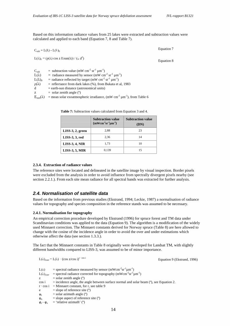
2.3.2. Conversion of digital numbers to physical unitsThe digital numbers, DNs, registered by the sensor were converted to at satellite radiance usingcalibration coefficients supplied by the data contractor (Table 5) and Equation 5.

Equation 5 (Markham and Barker, 1987)L( � = [/� �PD[��/� �PLQ@� �� minDNmax

�� = spectral radiance (mW cm-2 sr-1 µm-1)�� max = maximum spectral radiance (mW cm-2 sr-1 µm-1) registered by the sensor�� min = minimum spectral radiance (mW cm-2 sr-1 µm-1) registered by the sensorDN = digital number, absolute calibrated by the distributorDnmax = maximum digital number


13

Table 5: Minimum and maximum spectral radiance registered by LISS-3 compared to correspondingvalues for TM. To be used in Equation 1. From Euro Map (LISS-3) and Markham and Barker, 1987(TM).

Band L(max)(mWcm-2sr-1 µm-1)

L(min)(mWcm-2sr-1µm-1)

LISS-3, 2, green 14,45 1,76

TM 2, green 29,68 - 0,28

LISS-3, 3, red 17,03 1,54

TM 3, red 20,43 - 0,12

LISS-3, 4, nir 17,19 1,09

TM 4, nir 20,68 - 0,15

LISS-3, 5, mir 2,42 0

TM 5, mir 2,719 0,037

Data was generally expressed in radiance values. However, in some operations it was more feasible toexpress data in digital numbers (correction for species composition). The atmospheric correction evenrequired reflectance values, Equation 6. Values of mean solar exoatmospheric irradiance for thedifferent channels were calculated from Wolfe and Zissis (1989) (Table 6). For the earth-sun distance atable value from September 1996 was used (Astrophysical & Planetary Sciences University ofColorado http://lyra.colorado.edu/sbo/astroinfo/hale-bopp/triangles.html).

Equation 6 (Markham and Barker, 1987)

Table 6: Mean values of the solar exoatmospheric irradiance within the bands ofLISS-3, calculated from Wolfe and Zissis (1989) and compared to correspondingvalues for TM (Markham and Barker, 1987).

IRS-1C LISS-3 Landsat TM

Band 2, green 175,2(0.52-0.59 µm)

182,9(0.52-0.60 µm)

Band 3, red 151, 4(0.62-0.68 µm)

155,7(0.63-0.69 µm)

Band 4, nir 107,4(0.77-0.86 µm)

104,7(0.76-0.90 µm)

Band 5, mir 22,3(1.55-1.70 µm)

21,7(1.55-1.75 µm)

2.3.3. Correction for atmospheric effectsIn the absence of relevant background reflectance values and meteorological and atmospherical data, thecorrection for atmospheric effects was accomplished with a dark object subtraction.

Bukata et al. (1983) measured water spectral radiance in water with very small concentrations of suspendedsediment and phytoplankton. In contrast to what is sometimes assumed, they discovered that even clear deepwater reflects a small proportion of the visible light. For the green and red wavelength bands the reflectancefound was 2,0 and 0,4 percent respectively.

� �� 2 ) / (cos z ��

� � = reflectance (%)�� = spectral radiance (mW cm-2 sr-1 µm-1)d = earth-sun distance (astronomical units)z = solar zenith angle (º)Esun� � = mean solar exoatmospheric irradiance, from Table 6 (mW cm-2 µm-1)


14

Based on this information radiance values from 25 lakes were extracted and subtraction values werecalculated and applied to each band (Equation 7, 8 and Table 7).

Equation 7

Equation 8

Table 7: Subtraction values calculated from Equation 3 and 4.

Subtraction value(mWcm-2sr-1µm-1)

Subtraction value

(DN)

LISS-3, 2, green 2,88 23

LISS-3, 3, red 2,36 14

LISS-3, 4, NIR 1,73 10

LISS-3, 5, MIR 0,139 15

2.3.4. Extraction of radiance valuesThe reference sites were located and delineated in the satellite image by visual inspection. Border pixelswere excluded from the analysis in order to avoid influence from spectrally divergent pixels nearby (seesection 2.2.1.). From each site mean radiance for all spectral bands was extracted for further analysis.

2.4. Normalisation of satellite dataBased on the information from previous studies (Ekstrand, 1994; Leckie, 1987) a normalisation of radiancevalues for topography and species composition in the reference stands was assumed to be necessary.

2.4.1. Normalisation for topographyAn empirical correction procedure developed by Ekstrand (1996) for spruce forest and TM data underScandinavian conditions was applied to the data (Equation 9). The algorithm is a modification of the widelyused Minnaert correction. The Minnaert constants derived for Norway spruce (Table 8) are here allowed tochange with the cosine of the incidence angle in order to avoid the over and under estimations whichotherwise affect the data (see section 1.3.3.).

The fact that the Minnaert constants in Table 8 originally were developed for Landsat TM, with slightlydifferent bandwidths compared to LISS-3, was assumed to be of minor importance.

Equation 9 (Ekstrand, 1996)

Csub = �� 0

�� 0 �� cos z �� 2)

Csub = subtraction value (mW cm-2 sr-1 µm-1)�� = radiance measured by sensor (mW cm-2 sr-1 µm-1)�� 0 = radiance reflected by target (mW cm-2 sr-1 µm-1)� � = reflectance from dark lakes (%), from Bukata et al, 1983

d = earth-sun distance (astronomical units)z = solar zenith angle (º)Esun� � = mean solar exoatmospheric irradiance, (mW cm-2 µm-1), from Table 6

�� corr �� · (cos z/cos i)r · cos i

�� = spectral radiance measured by sensor (mWcm-2sr-1µm-1)�� corr = spectral radiance corrected for topography (mWcm-2sr-1µm-1)z = solar zenith angle (º)cos i = incidence angle, the angle between surface normal and solar beam (º), see Equation 2.r · cos i = Minnaert constant, for r, see table 9e = slope of reference site (º)

s = solar azimuth angle (º)n = slope aspect of reference site (º)s - n = ‘relative azimuth’ (º)


15

Table 8: Minnaert constants to be employed in Equation 9 (Ekstrand 1996).

Spectral band Minnaert constant

LISS-3, 2, green 0,34 · cos i

LISS-3, 3, red 0,56 (relative azimuth 0-90º)

0,36 (relative azimuth 91-180º)

LISS-3,4, NIR 1,04 · cos i (relative azimuth 0-60º)

0,97 · cos i (relative azimuth 61-180º)

LISS-3, 5, MIR 0,94 · cos i

2.4.2. Normalisation for species compositionReference data was not sufficient for a thorough study of the spectral effect of a variation in speciescomposition. Instead correction coefficients derived by Ekstrand (1994) were modified and used.

To obtain at least some information on the general radiometric level in the LISS-3 scene compared to theLandsat TM scene on which the correction coefficients previously had been used, DN values from the twodata sets were compared. Five deciduous stands (100 percent) were also located in both data sets. Digitalnumbers for each of the spectral bands were extracted and the digital numbers for these sites, as well as allthe reference sites, were plotted against corresponding deciduous components. The resulting regression lineswere studied and correction coefficients were derived (see section 3.1.2).

Satellite data was finally normalised using the correction coefficients and data on species composition fromthe air photo survey (Equation 10).

Equation 10 (Ekstrand, 1996)

2.5. Correlation between spruce defoliation and LISS-3 dataHalf of the reference sites were selected for use in the correlation analysis and remaining sites were left forevaluation. The selection was stratified in respect to defoliation levels in order to have a wide range ofdefoliation levels in both data sets.

The relationship between satellite data and defoliation was examined with regression analysis. Correlationcoefficients between defoliation and single spectral bands, as well as a number of indices were calculatedboth for corrected and non-corrected data.

The correlation coefficient is a measure of the strength of the relationship between two sets of variables.The stronger the relation, the closer the correlation coefficient is to 1. Whether the relation is a matter ofchance or not is described by the statistical significance. Significance at the 0,05 level for 30 observationsrequires a correlation coefficient of 0,306, and at the 0,01 level 0,432 (Hammond and McCullagh, 1978).

2.6. Defoliation assessment algorithm and verificationThe regression equation yielding highest correlation between satellite data and defoliation was inverted andused as an assessment algorithm. The assessment algorithm was verified by regression analysis of observedversus predicted defoliation of the verification data set. Defoliation of the sites not used in the correlationanalysis was predicted with the assessment algorithm and plotted against the levels observed in the air photointerpretation.

DNcorr ( ) = DN ( � – Cp( � P – Cd( � D

DN�� = digital number normalised for topography

DNcorr�� = digital number, corrected for pine and deciduous species components

P = pine component (%)

D = deciduous species component (%)

Cp( � = correction coefficient for the pine element

Cd( � = correction coefficient for the deciduous species element


16

3. Results and discussion

Visual inspection of the image data revealed a systematic striping within the visible and middle infraredbands, most apparent against dark backgrounds such as lakes. In Fourier spectra the stripes were clearlyseen as a narrow band from the upper left part of the spectra to the lower right side, indicating stripesstretching from north-east to south-west in the images, i.e. along the satellite track.

Striping effects in LISS-3 data have been reported from other authors as well. The origin of the striping ispresumably an imbalance in the radiometric response of the CCD elements. Several destriping proceduresexist. Although the pixel values by no means are raw; they have been subjected to calibration at the groundstation as well as geometric correction, it was thought inappropriate to interfere with the digital numbers asthe exact cause of the stripes were not known.

3.1. Normalisation of satellite data

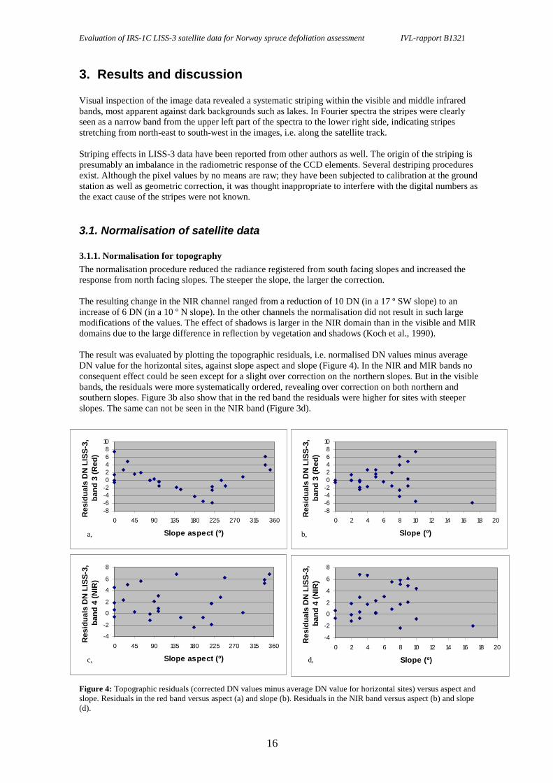
3.1.1. Normalisation for topography The normalisation procedure reduced the radiance registered from south facing slopes and increased theresponse from north facing slopes. The steeper the slope, the larger the correction. The resulting change in the NIR channel ranged from a reduction of 10 DN (in a 17 º SW slope) to anincrease of 6 DN (in a 10 º N slope). In the other channels the normalisation did not result in such largemodifications of the values. The effect of shadows is larger in the NIR domain than in the visible and MIRdomains due to the large difference in reflection by vegetation and shadows (Koch et al., 1990). The result was evaluated by plotting the topographic residuals, i.e. normalised DN values minus averageDN value for the horizontal sites, against slope aspect and slope (Figure 4). In the NIR and MIR bands noconsequent effect could be seen except for a slight over correction on the northern slopes. But in the visiblebands, the residuals were more systematically ordered, revealing over correction on both northern andsouthern slopes. Figure 3b also show that in the red band the residuals were higher for sites with steeperslopes. The same can not be seen in the NIR band (Figure 3d). Figure 4: Topographic residuals (corrected DN values minus average DN value for horizontal sites) versus aspect andslope. Residuals in the red band versus aspect (a) and slope (b). Residuals in the NIR band versus aspect (b) and slope(d).

-4

-2

0

2

4

6

8

0 45 90 135 180 225 270 315 360

Slope aspect (º)

Res

idu

als

DN

LIS

S-3

, b

and

4 (

NIR

)

-4

-2

0

2

4

6

8

0 2 4 6 8 10 12 14 16 18 20

Slope (º)

Res

idu

als

DN

LIS

S-3

, b

and

4 (

NIR

)

c, d,

-8-6-4-202468

10

0 45 90 135 180 225 270 315 360

Slope aspect (º)

Res

idu

als

DN

LIS

S-3

, b

and

3 (

Red

)

a,

-8-6-4-202468

10

0 2 4 6 8 10 12 14 16 18 20

Slope (º)

Res

idu

als

DN

LIS

S-3

, b

and

3 (

Red

)

b,


17

In Ekstrand (1993) residuals of estimated versus observed needle loss were plotted against slope. Althoughthis is not fully comparable to the present case, it is interesting to see that the residuals in that study werelarger on near horizontal than on steep slopes. The author explained this by the possibility that it is moredifficult to measure aspect on near horizontal slopes, and that this may introduce larger errors in these sites. It is important to bear in mind that the topographic residuals may be caused not only by a faulty correction,but also by variations in defoliation level and species composition. Perhaps also by variations in otherparameters such as age, density and atmospheric aerosols. However, residuals remaining due to otherfactors than an unsuccessful correction would be randomly scattered, unless the factor causing the residualsis biased for certain aspects or slopes. Despite the somewhat over corrected data the results from thecorrelation analysis (section 3.2) proved that the topographic normalisation was successful. 3.1.2. Normalisation for species compositionFigure 5 show the spectral effect of a varying deciduous component on Landsat TM 4 and the LISS-3bands.

Figure 5: Digital numbers plotted against percentdeciduous species in forest stands; the near infraredband of Landsat TM (a), the near infrared band ofLISS-3 (b), the green band of LISS-3 (c), the red bandof LISS-3 (d) and the MIR band of LISS-3 (e).

30

35

40

45

0 20 40 60 80 100

% deciduous trees

DN

, LIS

S-3

, ban

d 3

(G

reen

)

20

30

40

50

60

70

80

0 20 40 60 80 100

% deciduous trees

DN

, LIS

S-3

, ban

d 4

(N

IR)

10

15

20

25

0 20 40 60 80 100

% deciduous trees

DN

, LIS

S-3

, ban

d 3

(R

ed)

20

25

30

35

40

45

50

55

60

0 20 40 60 80 100

% deciduous trees

DN

, LIS

S-3

, ban

d 5

(M

IR)

20

30

40

50

60

70

80

90

0 20 40 60 80 100

% deciduous trees

DN

, TM

4 (

NIR

)

a,

e,

d,c,

b,


18

It is difficult to say anything about Figure 5 since no stand with a deciduous content within the range of 20and 100 percent exists. In the NIR bands a correlation can clearly be seen though, but whether it is a linearor non-linear relationship is impossible to say. In the study where the original correction constants weredeveloped (Ekstrand, 1993), a high correlation was found between percent deciduous trees and the NIRband, a lower correlation with the MIR band, and principally no relation with the visible bands. A similarresult was obtained by Leckie (1987).

Although the spectral effect of an increasing deciduous component in the visible bands (Figure 4e) does notappear to be less than the effect in the MIR band, it is not very strong and no correction for species contentwas attempted for data from these bands. No study of Swedish forests has revealed a good correlationbetween needle loss and data from visible wavelengths. The correction was hence concentrated on data fromthe infrared bands.

While DN values for stands with different deciduous species content ranged from 20 to approximately 70 inthe NIR band of TM, they ranged from approximately 25 to 60 in the LISS-3 NIR band (Figure 5).Corresponding values for the MIR band of LISS-3 were 28 to 50. A major reason why the range in LISS-3NIR data was narrower than in the TM NIR data, was thought to be the difference in sun elevation. Whereasthe TM scene was captured in early September, at a sun elevation of 33 degrees, the LISS data wasregistered at an elevation of 26 degrees in the end of September. Accordingly, correction coefficients weredetermined by calculating the ratio between the sun elevations of the two data sets, and multiply the originalcoefficients developed for TM NIR data with the ratio. The resulting coefficients are shown in Table 9.

Table 9: Correction coefficients for pine and deciduous components.

Correction coefficient,

Pine (DN)

Correction coefficient,

Deciduous (DN)

LISS-3, 4, NIR 0,04 0,1

LISS-3, 5, MIR 0,02 0,06

It may seem strange that the correction coefficients do not reflect the slopes of the regressions in Figure4b,e. The reason for this is may be that the relation between deciduous content in a spruce stand andsatellite-registered radiance is not linear. Maximum reduction of DN:s due to normalisation for species composition was 2 DN. The effect of thecorrection for species composition on radiance values is hence less than the correction for topography. Noreference stand was composed of 100 percent spruce, and it was not possible to evaluate the correction bycalculating residuals, i.e. corrected values subtracted by the value from 100 percent spruce stands. However,the results from the correlation analysis (section 3.2.) indicated that the species correction failed.

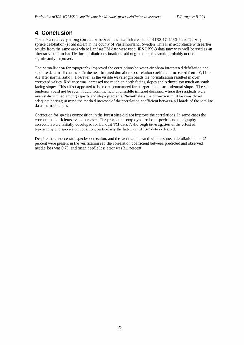
3.2. Correlation between spruce defoliation and LISS-3 data The NIR band alone appears to be best correlated with defoliation (Table 10, Figure 6). This is inaccordance with a number of studies (Brockhaus et al., 1992; Ekstrand, 1994; Ekstrand, 1998; Koch et al.,1990) although other authors have found highest correlation with MIR data and indices involving both NIRand MIR, or red, data (see section 1.2.). With the low resolution of the LISS-3 MIR channel in mind the lowcorrelations with the MIR-band and indices involving the MIR-band, is not a surprise. In previous studies where similar correction procedures as in the present study were employed, thecorrelation between defoliation and the NIR band of Landsat TM reached -0,80 (the same study area) and- 0,81 (south-west of Sweden) (Ekstrand, 1998). Brockhaus et al. (1992) studied defoliation in spruce-firdominated forests of North Carolina. They found a correlation of - 0,81 with TM 4 (NIR) and - 0,74 withSPOT HRV 3 (NIR). When data was normalised for elevation the correlations increased to -0,93 and -0,89respectively.


19

The correlation coefficients in this study were significantly higher for corrected than non-corrected data inall bands. This clearly shows the importance of correcting data for topographic effects. The correction forspecies composition did not affect the correlation coefficient particularly. It even resulted in a minor declineof the correlation, indicating that the normalisation procedure did not succeed in correcting for speciescomposition. A correction employing larger correction constants were tested, but did not result in highercorrelations. As have previously been discussed, the correlation between the content of pine and deciduoustrees in a spruce stand and reflectance may be non-linear. There is a need for a thorough investigation of theeffect of species composition on IRS data. Correction coefficients developed specifically for IRS datawould probably yield a better result. Table 10: Correlation between spruce defoliation and LISS-3 spectral bands and ratios.

Spectral band or ratio Correlation coefficient, rraw data

Correlation coefficient, rcorrected data1

Correlation coefficient, rcorrected data2

band 2(green) 0,14 -0,52 -0,52

band 3 (red) 0,25 -0,41 -0,41

band 4 (NIR) -0,19 -0,83 -0,82

band 5 (MIR) 0,006 -0,33 -0,31

Bands 5/4 0,29 0,31

Bands 4/3 0,33 0,33

NDVI (b4-b3/b4+b3) 0,42 0,421 Normalised for terrain effects only.2 Normalised for terrain effects and for pine and deciduous components.

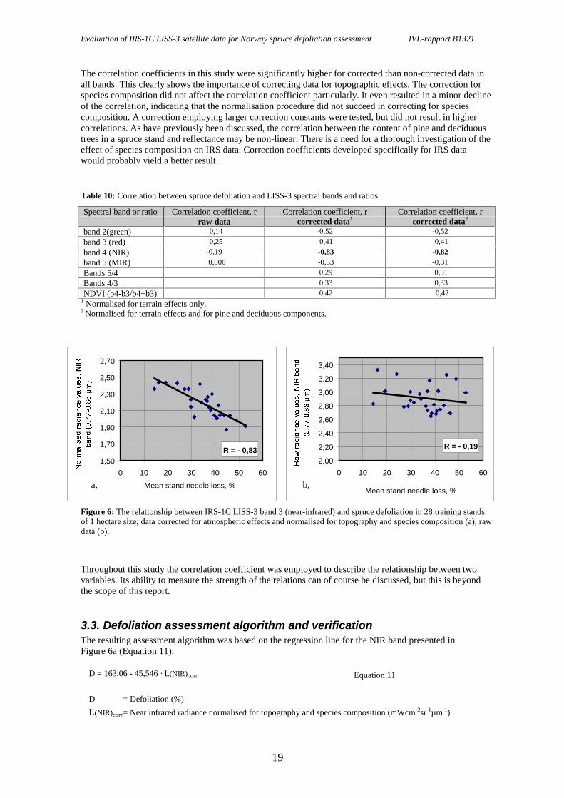
Figure 6: The relationship between IRS-1C LISS-3 band 3 (near-infrared) and spruce defoliation in 28 training standsof 1 hectare size; data corrected for atmospheric effects and normalised for topography and species composition (a), rawdata (b).

Throughout this study the correlation coefficient was employed to describe the relationship between twovariables. Its ability to measure the strength of the relations can of course be discussed, but this is beyondthe scope of this report.

3.3. Defoliation assessment algorithm and verificationThe resulting assessment algorithm was based on the regression line for the NIR band presented inFigure 6a (Equation 11).

Equation 11

R = - 0,831,50

1,70

1,90

2,10

2,30

2,50

2,70

0 10 20 30 40 50 60

Mean stand needle loss, %

R = - 0,19

2,00

2,20

2,40

2,60

2,80

3,00

3,20

3,40

0 10 20 30 40 50 60

Mean stand needle loss, %a, b,

D = 163,06 - 45,546 · L(NIR)corr

D = Defoliation (%)

L(NIR)corr= Near infrared radiance normalised for topography and species composition (mWcm-2sr-1µm-1)


20

Despite the fact that there were no sites with less than 25 percent mean needle loss in the verification set,the correlation between predicted and observed defoliation was 0,70 (Figure 7). Root mean square was 3,1percent needle loss.

Figure 7: Observed versus predicted defoliation in reference sites used for evaluation.

The majority of stands in Västernorrland have a mean needle loss in the range of 20 to 45 percent. Onlythree sites had lower values, but these were needed for the correlation analysis. A fact that may affect theprediction of defoliation in the verification sites is that slope and aspect were estimated from air photos andnot in field. However, in an operational context slope and aspect would be derived from a digital elevationmodel, which presumably would yield a slightly lower correlation.

3.4. IRS LISS-3 versus Landsat TMThis study indicates that the performance of IRS LISS-3 for defoliation studies of Norway spruce (Piceaabies) is comparable to that of Landsat TM. It could very well be used as an alternative to TM data, whichwould significantly increase the possibility to obtain cloud free satellite data.

However, there are a couple of reasons why data from the TM sensor may be preferred. One is that thesensor has been in use for a quite long time and much research has been made on its performance, e.g. thecalibration of the sensor is better known and studies of its decay with time has been performed. Anotherreason is that the radiometric performance of TM appears to be better. It registers the electromagneticradiation in an 8-bit resolution while LISS-3 registers in 7 bits. Channel offsets are also higher in LISS-3than in TM (Table 5) which means that the dynamic range of the sensor is lower than for Landsat TM. Thismay be important in defoliation studies where relatively low values of radiance are considered. However, itmay also be that the sensitivity of LISS-3 is concentrated on the most interesting radiance interval so thatthe lower dynamic range does not affect the defoliation assessment at all.

3.5. Error sources

3.5.1. Delineation of reference sites in the satellite scene.Delineation of reference sites in the satellite scene was performed manually. Choosing which pixels shouldbe included and which should not, is a critical and subjective step of the study.

An alternative would have been to calculate map co-ordinates for the sites from the aerial photographs, andthen add them to the satellite in an overlay process. However the total Root Mean Square Error, RMSE, forthe geometric correction was 10,3 m., i.e. less than one pixel. Maximum RMSE for a single GCP was 15 m.Better accuracy is rarely achieved. Still the geometric displacement may locally be as high as one pixel, andan arbitrary displacement of one pixel could have detrimental effects on the defoliation assessments.

15

20

25

30

35

40

45

50

15 20 25 30 35 40 45 50

Observed defoliation (%)


21

3.5.2. Correction for varying forest stand parametersCorrection for pine and deciduous components was achieved using correction coefficients empiricallyderived from another data set. Although the coefficients were modified based on the difference in sunelevation between the two data sets, a proper procedure would have been to develop completely newcoefficients from the IRS data set. This however required a large number of stands with varying degrees ofpine and deciduous components but very narrow ranges of age, density and defoliation, and such a data setwas not available.

Age and density were attended by excluding stands older than 70 years as well as sparse stands from thestudy. This was performed by visual inspection of air photos. The resolution of the air photos was high andonly minor errors are likely to have been introduced. Forest younger than 70 years is rarely affected bydefoliation in the region, and defoliation assessments of these stands are not really urgent. Stands with lowdensities may occur despite that most forests in Sweden are used in production and are intensively managed.Even though they do not occur very frequently, it would be good to be able to assess defoliation also instands with low densities. While in this study only selected stands were studied, an operational contextrequires a more automatic approach to obtain information of age and density of the forest. Ekstrand (1996,1998) has integrated digital forest maps with satellite data to obtain information on forest parameters. Butdigital forest maps do not exist over all forests, and are time and cost consuming to produce. It will thus beinteresting to see which potential the forthcoming high-resolution satellite data has for classification offorest parameters such as age, density (and gaps) and species.

3.5.3. Correction for topographyThe topographic normalisation algorithm employed in the study was also originally developed for LandsatTM data. A procedure optimised for LISS-3 should be produced when a sufficiently extensive referencedata set is available.

3.5.4. Errors in reference dataEkstrand (1991) examined the accuracy of air photo interpreted estimations of defoliation (on a scale of1:6000). He found that 71 % of 100 trees were classified into the correct class. However, when comparingthe mean values of the interpreted defoliation with the mean value of the field assessment, they were verysimilar; 32,5 versus 29,9 percent.

The accuracy of species interpretation in 1:6000 air photos, is approximately 95 percent for pine trees and100 percent for deciduous trees (Ekstrand 1993).

3.5.5. Radiometric correctionThe absolute values of radiance presented in the study should be considered with caution. Conversion ofdigital numbers to at satellite radiance was based on calibration data from the contractor. The author doesnot know exactly how these calibration coefficients were produced, but according to EuroMap (Zahn, C.personal communication, 1998) no post-launch calibration campaign has been performed. This means thatno account has been taken to the decay of the sensor with time. Moran et al. (1995) have studied thedecreasing response with time for the Landsat TM and SPOT HRV sensors. They found a sharp decrease inresponse shortly after launch in both sensors.

Correcting for atmospheric effects with a dark object subtraction is a rather rough approach. A proper set ofinput to the widely used 6S software (Second Simulation of Satellite Signal in the Solar Spectrum) isgenerally thought to give a better correction for atmospheric disturbances (Alm, personal comunication,1998). However, with the assumption of a homogene atmosphere the atmospheric correction does notinfluence correlations and regressions based on single bands, but only ratios and spectral profiles. Theassumption of a homogenous atmosphere is rarely valid though, but data on aerosol and water content witha sufficient spatial resolution is not available in Sweden.


22

4. ConclusionThere is a relatively strong correlation between the near infrared band of IRS-1C LISS-3 and Norwayspruce defoliation (Picea abies) in the county of Västernorrland, Sweden. This is in accordance with earlierresults from the same area where Landsat TM data were used. IRS LISS-3 data may very well be used as analternative to Landsat TM for defoliation estimations, although the results would probably not besignificantly improved.

The normalisation for topography improved the correlations between air photo interpreted defoliation andsatellite data in all channels. In the near infrared domain the correlation coefficient increased from –0,19 to-82 after normalisation. However, in the visible wavelength bands the normalisation resulted in overcorrected values. Radiance was increased too much on north facing slopes and reduced too much on southfacing slopes. This effect appeared to be more pronounced for steeper than near horizontal slopes. The sametendency could not be seen in data from the near and middle infrared domains, where the residuals wereevenly distributed among aspects and slope gradients. Nevertheless the correction must be consideredadequate bearing in mind the marked increase of the correlation coefficient between all bands of the satellitedata and needle loss.

Correction for species composition in the forest sites did not improve the correlations. In some cases thecorrection coefficients even decreased. The procedures employed for both species and topographycorrection were initially developed for Landsat TM data. A thorough investigation of the effect oftopography and species composition, particularly the latter, on LISS-3 data is desired.

Despite the unsuccessful species correction, and the fact that no stand with less mean defoliation than 25percent were present in the verification set, the correlation coefficient between predicted and observedneedle loss was 0,70, and mean needle loss error was 3,1 percent.


23

References

Alm, G., 1998. Personal communication. Department of Physical geography, Stockholm university,Sweden.

Ardö, J., 1998. Remote sensing of forest decline in the Czech Republic. Ph.D. thesis, Lund university, Lund,Sweden.

Berghäll, S., Wijk, S., Wulff, S. and Söderberg, U. 1995. Skogsskador i Sverige 1994. Resultat avskogsskadebevaknsing från riksskogstaxeringen och skogsvårdsorganisationens observationsytor.Skogsstyrelsen, Rapport 1995:4, Skogsstyrelsens förlag, Jönköping, Sweden.

Brockhaus, J.A., Khorram, S., Bruck, R.I., Campbell, M.V. and Stallings, C., 1992. A comparison ofLandsat TM and SPOT HRV data for use in the development of forest defoliation models. InternationalJournal of Remote Sensing 13(16): 3235-3240.

Bukata, R. R., Bruton, J.E. and Jerome, J.H., 1983. Use of chromaticity in remote measurements of waterquality, Remote Sensing Environment 13:161-177.

Chavez, P.S.,Jr., 1988. An improved dark-object subtraction technique for atmospheric scattering correctionof multispectral data. Remote Sensing Environment 24:459-479.

Civco, D.L., 1989. Topographic normalization of Landsat Thematic Mapper digital imagery.Photogrammetric Engineering and Remote Sensing 55(9): 1303-1309.

Colwell, J.E., 1974. Vegetation canopy reflectance. Remote Sensing Environment 3:175-183.

Deering, D.W. Middleton, E.M. and Eck, T.F., 1994. Reflectance anisotropy for spruce-hemlock forestcanopy. Remote Sensing Environment 47:242-260.

Ekstrand, S., 1991. Effekter av luftföroreningar från vägtrafik på närliggande skog. Flygbildsbedömning avkronutglesning på gran. IVL-report B-1016, Stockholm, Sweden.

Ekstrand, S., 1993. Assessment of forest damage with Landsat TM, elevation models and digital forestmaps. Ph.D. thesis, Royal Institute of Technology, Stockholm, Sweden.

Ekstrand, S., 1994. Assessment of forest damage with Landsat TM: Correction for varying forest standcharacteristics. Remote Sensing Environment 47:291-302.

Ekstrand, S., 1996. Landsat TM based forest damage assessment Correction for topographic effects.Photogrammetric Engineering and Remote Sensing 62(2), 151-161.

Ekstrand, S. and Hansen, C., 1998. Pilot study on the use of satellite data for regional forest conditionsurveys. Proj. no. 96.60.SW.004.0. IVL-report B-1281, Stockholm, Sweden.

Franklin, J., 1986. Thematic Mapper analysis of coniferous forest structure and composition. InternationalJournal of Remote Sensing 7:1287-1301.

Hammond, R. and McCullough, P.S., 1978. Quantitative techniques in geography: an introduction, 2nd ed.Oxford University Press, 364 pp.

Heikkilä, J. 1998. Monitoring boreal coniferous forest health in Finland using the reference sample plotmethod with multisource and multitemporal data. Fil. Lic. Thesis, University of Joensuu, Finland.

Häusler, T., 1991. Waldschadenkartierung in Fichtenrevieren durch Auswerung von Satellitenaufnahmenund raumbezogenen Zusatzdaten, Dissertation Uni Freiburg, Germany. [Mapping forest damages in Norwayspruce areas by analysing satellite images and ancillary data].

Hällgren, J-E., 1995. Skogstillväxt – klimat. In: Kritiska faktorer för skogsträdens tillväxt och vitalitet,Konferens den 29 mars 1995 anordnad av sitftelsen Svensk växtnäringsforskning., Agerlid, G., (ed). Kungl.Skogs- och lantbruksakademien, Sweden.

Kalyanaraman, S., Rajangam, R.K. and Rattan, R.,1995. Indian remote sensing spacecraft – 1C/1D.International Journal of Remote Sensing 16:791-799.

Kaufman, Y.J. and Tanré, D., 1996. Strategy for direct and indirect methods for correcting the aerosol effecton remote sensing: from AVHRR to EOS-MODIS. Remote Sensing Environment 55:65-79.


24

Kawata, Y., Ueno, S. and Kusaka, T., 1988. Radiometric correction for atmospheric and topographic effectson Landsat MSS images. International Journal of Remote Sensing 9(4):729-748.

Kleman, J., 1986. The spectral reflectance of stands of Norway spruce and Scotch pine, measured from ahelicopter. Remote Sensing of Environment 20:253-256.

Koch, B., Ammer, U., Schneider, T. and Wittmeier, H.,1990. Spectroradiometer measurements in thelaboratory and in the field to analyse the influence of different damage symptoms on the reflection spectraof forest trees. International Journal of Remote Sensing 11(7), 1145-1163.

Kowalik, W.S., Lyon, R.J.P and Switzer, P., 1983. The effects of additive radiance terms on ratios ofLandsat data. Photogrammetric Engineering and Remote Sensing 49(5):659-669.

Kriebel, K.T., 1976. On the variability of reflected radiation field due to differing, distributions of theirratiation. Remote Sensing of Environment 4:257-264.

Lambert, N.A., Ardö, J., Rock, B.N. and Vogelman, J.E., 1995. Spectral characterization and regression-based classification of forest damage in Norway spruce stands in the Czech Republic using LandsatThematic Mapper data. International Journal of Remote Sensing 16(7), 1261-1287.

Leckie, D.G., 1987. Factors affecting defoliation assessment using airborne multispectral scanner data.Photogrammetric Engineering and Remote Sensing 53(12): 1665-1674.

Leckie, D.G., Teillet, P.M., Fedosejevs, G. and Ostaff, D.P., 1988. Reflectance characteristics of cumulativedefoliation of balsam fir. Canadian Journal of Forest Research 18:1008-1016.

Lillesand, T.M. and Kiefer, R.W., 1994. Remote sensing and image interpretation, 3rd ed, Wiley and sons,USA, 729 pp.

Markham, B.L. and Barker, J.L., 1987. Thematic Mapper bandpass solar exoatmospheric irradiances.International Journal of Remote Sensing 8(3), 517-523.

Meyer, P., Itten, K.I., Kellenberger, T. Sandmeier, S. and Sandmeier, R., 1993. Radiometric corrections oftopographically induced effects on Landsat TM data in an alpine environment. ISPRS Journal ofPhotogrammetry and Remote Sensing 48(4):17-28.

Minnaert, M., 1941. The reciprocitiy principle in lunar photometry. Astrophysical Journal 93:403-410.

Moran, M.S., Jackson, R.D., Clarke, T.R., Qi, J., Cabot, F., Thome, K.J. and Markham, B.L., 1995.Reflectance factor retrieval from Landsat TM and SPOT HRV data for bright and dark targets. RemoteSensing of Environment 52:218-230.

National Forest Inventory, 1998. Skogsdata. Excel data on forest taxations 1992-1996, Institutionen förskoglig resurshushållning och geomatik, SLU, Umeå, Sweden.

Nihlgård, B., 1996. Skogsskadornas mångfaldiga bakgrund. Skog och forskning 3:6-12.

Rock, B., Hoshizaki, T. and Miller, J.R., 1988. Comparison of in-situ and airborne spectral measurement ofthe blue shift associated with forest damage. Remote Sensing of Environment 24:109-127.

Schulze, E-D., 1989. Air pollution and forest decline in a spruce (Picea abies) forest. Science, 244: 776-783.

Smith, J.A., Lin, T.L. and Rasnson, K.J. 1980. The Lambertian assumptionand Landsat data.Photogrammetric Engineering and Remote Sensing 46(9): 1183-1189.

Swain, P. H. and Davis, S.M. (eds), 1978. The quantitative approach, Chapt. 5, McGraw-Hill, New York, .

Teillet, P.M., Guindon, B. and Goodenough, D.G., 1982. On the slope-aspect correction of multispectralscanner data. Canadian Journal of Remote Sensing 8(2):84-106.

Thomson, A.G. and Jones, C., 1990. Effects of topography on radiance from upland vegetation in NorthWales. International Journal of Remote Sensing 11(5):829-840.

Vogelmann, J.E. and Rock, B.N., 1988. Assessing forest damage in high-elevation coniferous forests inVermont and New Hampshire using Thematic Mapper data. Remote Sensing of Environment 24:227-246.

Vogelmann, J.E., 1990, Comparison between two vegetation indices for measuring different types of forestdamage in the nort-eastern United States. International Journal of Remote Sensing 12:2281-2297.


25

Wastenson, L., Alm, G., Kleman, J. and Wastenson, B., 1987. Swedish experiences on forest damageinventory by remote sensing methods. International Journal of Aerial and Space Imaging, Remote sensingand Integrated Geographical Systems 1(1):43-52.

Wolfe, W.L. and Zissis, G.J., 1989. The infrared handbook. The infrared information analysis center,Environmental research institute of Michigan.

Wulff, S. and Löfgren, O., 1998. Instruktion för fältarbetet vid riksskogstaxeringens skogsskadeinventeringår 1998. Institutionen för skoglig resurshushållning och geomatik, Umeå.

Yugui, Z.,1989. Normalization of Landsat TM imagery by atmospheric correction for forest scenes inSweden. Research Report, Remote Sensing Laboratory, Swedish University of Agriculture Sciences, Umeå.

Zahn, C., 1998. Personal communication. Euromap, Germany.

IVL Svenska Miljöinstitutet AB IVL Swedish Environmental Research Institute Ltd

Box 210 60, SE-100 31 StockholmHälsingegatan 43, StockholmTel: +46 8 598 563 00Fax: +46 8 598 563 90

Box 470 86, SE-402 58 GöteborgDagjämningsgatan 1, GöteborgTel: +46 31 725 62 00Fax: +46 31 725 62 90

Aneboda, SE-360 30 LammhultAneboda, LammhultTel: +46 472 26 20 75Fax: +46 472 26 20 04

www.ivl.se

˘ ˇˆ - gisresources.com˜ ˇˆ ˙ ˝ ˛ helén falkenström b 1321 stockholm, february 1999 r = -...

Documents