downloads.hindawi.comdownloads.hindawi.com/journals/specialissues/521580.pdf · editorial board...
TRANSCRIPT

Numerical and Analytical Methods for Variational Inequalities and Related Problems with Applications
Journal of Applied Mathematics
Guest Editors: Zhenyu Huang, Ram N. Mohapatra, Muhammad Aslam Noor, Hong-Kun Xu, and Qingzhi Yang

Numerical and Analytical Methods forVariational Inequalities and RelatedProblems with Applications

Journal of Applied Mathematics
Numerical and Analytical Methods forVariational Inequalities and RelatedProblems with Applications
Guest Editors: Zhenyu Huang, Ram N. Mohapatra,Muhammad Aslam Noor, Hong-Kun Xu,and Qingzhi Yang

Copyright q 2012 Hindawi Publishing Corporation. All rights reserved.
This is a special issue published in “Journal of Applied Mathematics.” All articles are open access articles distributed underthe Creative Commons Attribution License, which permits unrestricted use, distribution, and reproduction in anymedium,provided the original work is properly cited.

Editorial BoardSaeid Abbasbandy, IranMina B. Abd-El-Malek, EgyptMohamed A. Abdou, EgyptSubhas Abel, IndiaMostafa Adimy, FranceCarlos J. S. Alves, PortugalMohamad Alwash, USAIgor Andrianov, GermanySabri Arik, TurkeyFrancis T. K. Au, Hong KongOlivier Bahn, CanadaRoberto Barrio, SpainAlfredo Bellen, ItalyJ. Biazar, IranHester Bijl, The NetherlandsJames Robert Buchanan, USAAlberto Cabada, SpainXiao Chuan Cai, USAJinde Cao, ChinaAlexandre Carvalho, BrazilSong Cen, ChinaQianshun S. Chang, ChinaShih-sen Chang, ChinaTai-Ping Chang, TaiwanKe Chen, UKXinfu Chen, USARushan Chen, ChinaEric Cheng, Hong KongFrancisco Chiclana, UKJen-Tzung Chien, TaiwanCheng-Sheng Chien, TaiwanHan Choi, Republic of KoreaTin-Tai Chow, ChinaS. H. Chowdhury, MalaysiaC. Conca, ChileVitor Costa, PortugalLivija Cveticanin, SerbiaAndrea De Gaetano, ItalyPatrick De Leenheer, USAEric de Sturler, USAOrazio Descalzi, ChileKai Diethelm, Germany
Vit Dolejsi, Czech RepublicMagdy A. Ezzat, EgyptMeng Fan, ChinaYa Ping Fang, ChinaAntonio Ferreira, PortugalMichel Fliess, FranceM. A. Fontelos, SpainLuca Formaggia, ItalyHuijun Gao, ChinaB. Geurts, The NetherlandsJamshid Ghaboussi, USAPablo Gonzalez-Vera, SpainLaurent Gosse, ItalyK. S. Govinder, South AfricaJose L. Gracia, SpainYuantong Gu, AustraliaZhihong Guan, ChinaNicola Guglielmi, ItalyFrederico G. Guimaraes, BrazilVijay Gupta, IndiaBo Han, ChinaMaoan Han, ChinaPierre Hansen, CanadaFerenc Hartung, HungaryTasawar Hayat, PakistanXiaoqiao He, Hong KongLuis Javier Herrera, SpainYing Hu, FranceNing Hu, JapanZhilong L. Huang, ChinaKazufumi Ito, USATakeshi Iwamoto, JapanGeorge Jaiani, GeorgiaZhongxiao Jia, ChinaTarun Kant, IndiaIdo Kanter, IsraelA. Kara, South AfricaJ. H. Kim, Republic of KoreaKazutake Komori, JapanFanrong Kong, USAVadim A. Krysko, RussiaJin L. Kuang, Singapore
Miroslaw Lachowicz, PolandHak-Keung Lam, UKTak-Wah Lam, Hong KongP. G. L. Leach, UKWan-Tong Li, ChinaYongkun Li, ChinaJin Liang, ChinaChong Lin, ChinaLeevan Ling, Hong KongChein-Shan Liu, TaiwanM. Z. Liu, ChinaZhijun Liu, ChinaYansheng Liu, ChinaShutian Liu, ChinaKang Liu, USAFawang Liu, AustraliaJulian Lopez-Gomez, SpainShiping Lu, ChinaGert Lube, GermanyNazim I. Mahmudov, TurkeyOluwole D. Makinde, South AfricaFrancisco J. Marcellan, SpainGuiomar Martın-Herran, SpainNicola Mastronardi, ItalyMichael McAleer, The NetherlandsStephane Metens, FranceMichael Meylan, AustraliaAlain Miranville, FranceJaime E. Munoz Rivera, BrazilJavier Murillo, SpainRoberto Natalini, ItalySrinivasan Natesan, IndiaJiri Nedoma, Czech RepublicJianlei Niu, Hong KongKhalida I. Noor, PakistanRoger Ohayon, FranceJavier Oliver, SpainDonal O’Regan, IrelandMartin Ostoja-Starzewski, USATurgut Ozis, TurkeyClaudio Padra, ArgentinaReinaldo M. Palhares, Brazil

Francesco Pellicano, ItalyJuan Manuel Pena, SpainRicardo Perera, SpainMalgorzata Peszynska, USAJames F. Peters, CanadaM. A. Petersen, South AfricaMiodrag Petkovic, SerbiaVu Ngoc Phat, VietnamAndrew Pickering, SpainHector Pomares, SpainMaurizio Porfiri, USAMario Primicerio, ItalyM. Rafei, The NetherlandsB. V. Rathish Kumar, IndiaJacek Rokicki, PolandDirk Roose, BelgiumCarla Roque, PortugalDebasish Roy, IndiaSamir H. Saker, EgyptMarcelo A. Savi, BrazilWolfgang Schmidt, GermanyEckart Schnack, GermanyMehmet Sezer, TurkeyNaseer Shahzad, Saudi Arabia
Fatemeh Shakeri, IranHui-Shen Shen, ChinaJian Hua Shen, ChinaFernando Simoes, PortugalTheodore E. Simos, GreeceA. A. Soliman, EgyptXinyu Song, ChinaQiankun Song, ChinaYuri N. Sotskov, BelarusPeter Spreij, The NetherlandsNiclas Stromberg, SwedenRay Su, Hong KongJitao Sun, ChinaWenyu Sun, ChinaXianHua Tang, ChinaMarco H. Terra, BrazilAlexander Timokha, NorwayMariano Torrisi, ItalyJung-Fa Tsai, TaiwanCh. Tsitouras, GreeceKuppalapalle Vajravelu, USAAlvaro Valencia, ChileErik Van Vleck, USAEzio Venturino, Italy
Jesus Vigo-Aguiar, SpainMichael N. Vrahatis, GreeceBaolin Wang, ChinaMingxin Wang, ChinaJunjie Wei, ChinaLi Weili, ChinaMartin Weiser, GermanyFrank Werner, GermanyShanhe Wu, ChinaDongmei Xiao, ChinaYuesheng Xu, USASuh-Yuh Yang, TaiwanWen-Shyong Yu, TaiwanJinyun Yuan, BrazilAlejandro Zarzo, SpainGuisheng Zhai, JapanZhihua Zhang, ChinaJingxin Zhang, AustraliaChongbin Zhao, AustraliaXiaoQiang Zhao, CanadaShan Zhao, USARenat Zhdanov, USAHongping Zhu, ChinaXingfu Zou, Canada

Contents
Numerical and Analytical Methods for Variational Inequalities and Related Problems withApplications, Zhenyu Huang, Ram N. Mohapatra, Muhammad Aslam Noor, Hong-Kun Xu,and Qingzhi YangVolume 2012, Article ID 684104, 2 pages
Approximations of Numerical Method for Neutral Stochastic Functional DifferentialEquations with Markovian Switching, Hua Yang and Feng JiangVolume 2012, Article ID 675651, 32 pages
Choosing Improved Initial Values for Polynomial Zerofinding in Extended Newbery Methodto Obtain Convergence, Saeid Saidanlu, Nor’aini Aris, and Ali Abd RahmanVolume 2012, Article ID 167927, 12 pages
The Spectral Method for the Cahn-Hilliard Equation with Concentration-Dependent Mobility,Shimin Chai and Yongkui ZouVolume 2012, Article ID 808216, 35 pages
Viscosity Approximation Methods for Equilibrium Problems, Variational Inequality Problemsof Infinitely Strict Pseudocontractions in Hilbert Spaces, Aihong WangVolume 2012, Article ID 150145, 20 pages
Integration Processes of Delay Differential Equation Based on Modified Laguerre Functions,Yeguo SunVolume 2012, Article ID 978729, 18 pages
Existence of Weak Solutions for Nonlinear Fractional Differential Inclusion withNonseparated Boundary Conditions, Wen-Xue Zhou and Hai-Zhong LiuVolume 2012, Article ID 530624, 13 pages
Well-Posedness by Perturbations for Variational-Hemivariational Inequalities, Shu Lv,Yi-bin Xiao, Zhi-bin Liu, and Xue-song LiVolume 2012, Article ID 804032, 18 pages
Convergence of Implicit and Explicit Schemes for an Asymptotically Nonexpansive Mappingin q-Uniformly Smooth and Strictly Convex Banach Spaces, Meng Wen, Changsong Hu,and Zhiyu WuVolume 2012, Article ID 474031, 15 pages
Strong Convergence of a Hybrid Iteration Scheme for Equilibrium Problems, VariationalInequality Problems and Common Fixed Point Problems, of Quasi-φ-AsymptoticallyNonexpansive Mappings in Banach Spaces, Jing ZhaoVolume 2012, Article ID 516897, 19 pages
A Hybrid Gradient-Projection Algorithm for Averaged Mappings in Hilbert Spaces, Ming Tianand Min-Min LiVolume 2012, Article ID 782960, 14 pages

Cyclic Iterative Method for Strictly Pseudononspreading in Hilbert Space, Bin-Chao Deng,Tong Chen, and Zhi-Fang LiVolume 2012, Article ID 435676, 15 pages
A Note on Approximating Curve with 1-Norm Regularization Method for the Split FeasibilityProblem, Songnian He and Wenlong ZhuVolume 2012, Article ID 683890, 10 pages
General Iterative Algorithms for Hierarchical Fixed Points Approach to VariationalInequalities, Nopparat Wairojjana and Poom KumamVolume 2012, Article ID 174318, 20 pages
The Modified Block Iterative Algorithms for Asymptotically Relatively NonexpansiveMappings and the System of Generalized Mixed Equilibrium Problems,Kriengsak Wattanawitoon and Poom KumamVolume 2012, Article ID 395760, 24 pages
OnMultivalued Nonexpansive Mappings in R-Trees, K. Samanmit and B. PanyanakVolume 2012, Article ID 629149, 13 pages
Global Dynamical Systems Involving Generalized f-Projection Operators and Set-ValuedPerturbation in Banach Spaces, Yun-zhi Zou, Xi Li, Nan-jing Huang, and Chang-yin SunVolume 2012, Article ID 682465, 12 pages
Global Error Bound Estimation for the Generalized Nonlinear Complementarity Problem overa Closed Convex Cone, Hongchun Sun and Yiju WangVolume 2012, Article ID 245458, 11 pages
A New Iterative Scheme for Solving the Equilibrium Problems, Variational InequalityProblems, and Fixed Point Problems in Hilbert Spaces,Rabian Wangkeeree and Pakkapon PreechasilpVolume 2012, Article ID 154968, 21 pages
Cubic B-Spline Collocation Method for One-Dimensional Heat and Advection-DiffusionEquations, Joan Goh, Ahmad Abd. Majid, and Ahmad Izani Md. IsmailVolume 2012, Article ID 458701, 8 pages
Analytic Solutions of Some Self-Adjoint Equations by Using Variable Change Method and ItsApplications, Mehdi Delkhosh and Mohammad DelkhoshVolume 2012, Article ID 180806, 7 pages
Algorithms for a System of General Variational Inequalities in Banach Spaces, Jin-Hua Zhu,Shih-Sen Chang, and Min LiuVolume 2012, Article ID 580158, 18 pages
Finite Difference Method for Solving a System of Third-Order Boundary Value Problems,Muhammad Aslam Noor, Eisa Al-Said, and Khalida Inayat NoorVolume 2012, Article ID 351764, 10 pages

Contents
Existence and Algorithm for Solving the System of Mixed Variational Inequalities in BanachSpaces, Siwaporn Saewan and Poom KumamVolume 2012, Article ID 413468, 15 pages

Hindawi Publishing CorporationJournal of Applied MathematicsVolume 2012, Article ID 684104, 2 pagesdoi:10.1155/2012/684104
EditorialNumerical and Analytical Methods forVariational Inequalities and Related Problemswith Applications
Zhenyu Huang,1 Ram N. Mohapatra,2 Muhammad Aslam Noor,3Hong-Kun Xu,4 and Qingzhi Yang5
1 Department of Mathematics, Nanjing University, Nanjing 210093, China2 Department of Mathematics, University of Central Florida, Orlando, FL 32816, USA3 Mathematics Department, COMSATS Institute of Information Technology, Islamabad, Pakistan4 Department of Applied Mathematics, National Sun Yat-Sen University, Kaohsiung 804, Taiwan5 School of Mathematics and LPMC, Nankai University, Tianjin 300071, China
Correspondence should be addressed to Zhenyu Huang, [email protected]
Received 23 October 2012; Accepted 23 October 2012
Copyright q 2012 Zhenyu Huang et al. This is an open access article distributed under theCreative Commons Attribution License, which permits unrestricted use, distribution, andreproduction in any medium, provided the original work is properly cited.
The study of variational inequalities and related problems with applications constitutes arich topic of intensive research efforts within the latest 50 years. Variational inequality theory,which was introduced by Stampacchia in 1964, has emerged as a fascinating branch ofmathematical and engineering sciences with a wide range of applications in industry, finance,economics, ecology, social, regional, pure, and applied sciences. The corresponding iterativemethods have witnessed great progress in recent years to handle problems in optimizationproblems, inverse problems, and differential equations.
We received 61 research papers in the research fields. This special issue includes 23high-quality peer-reviewed papers. The aim of this special issue has been to present the latestand generalized coverage of the fundamental and constructive ideas, concepts, and importantissues in the accepted original research articles as well as comprehensive review articlesstimulating the continuing efforts to numerical analysis for variational inequality problemsand fixed-point problems with applications.
In the fascinating paper by S. Saewan and P. Kumam, the existence and convergenceanalysis of the solutions of system of mixed variational inequalities in Banach spacesare given by using the generalized projection operator. N. Wairojjana and P. Kumamprovide several general iterative methods for finding the solutions to variational inequalities.Modified block iterative methods are presented by K. Wattanawitoon and P. Kumamfor asymptotically relatively nonexpansive mappings and for systems of generalizedmixed equilibriums. In the setting of Hilbert spaces, several distinguished researchers,

2 Journal of Applied Mathematics
R. Wangkeeree and P. Preechasilp; K. Wattanawitoon and P. Kumam; A. Wang, areworking successfully on finding the common solutions to various equilibrium problems,variational inequalities, and fixed point problems. For the more general Banach spaces, thecorresponding problems are studied by distinguished people such as J.-H. Zhu et al. intheir original independent work. Seven published papers work on the related differentialequations and applications. In the interesting paper by M. A. Noor et al., the relationshipbetween differential equations and general variational inequalities is established withnumerical methods. These wonderful results in the studies of differential equations aregiven independently by S. Chai and Y. Zou; Y. Sun; W.-X. Zhou and H.-Z. Liu; J. Gohetal.; M. Delkhosh and M. Delkhosh; H. Yang and F. Jiang. Eight published papers havegood studies on providing solutions to the complementarity problems by H. Sun andY. Wang; properties for multivalued nonexpansive mappings in R-trees by K. Samanmitand B. Panyanak; iterative methods for strict pesudocontractions by B.-C. Deng et al.; 1-norm regularization method for split feasibility problems by S. He and W. Zhu; gradient-projection algorithms for averaged mappings by M. Tian and M.-M. Li; implicit and explicitalgorithms for asymptotically nonexpansive mappings by M. Wen et al.; well-posedness forhemivariational inequalities by S. Lv et al.; improved initial values for polynomial zeros byS. Saidanlu et al.
Acknowledgments
The Editors would like to express their deepest gratitude to the authors for their fascinatingand interesting contributions as well as to the staff and the editorial office of the journalfor the great and invaluable support. The Editors would like also to express theirgreatest appreciation to more than 200 reviewers for their important time and valuablesuggestions/comments to make the special issue successful with highly qualified publishedpapers.
Zhenyu HuangRam N. Mohapatra
Muhammad Aslam NoorHong-Kun XuQingzhi Yang

Hindawi Publishing CorporationJournal of Applied MathematicsVolume 2012, Article ID 675651, 32 pagesdoi:10.1155/2012/675651
Research ArticleApproximations of Numerical Method for NeutralStochastic Functional Differential Equations withMarkovian Switching
Hua Yang1 and Feng Jiang2
1 School of Mathematics and Computer Science, Wuhan Polytechnic University, Wuhan 430023, China2 School of Statistics and Mathematics, Zhongnan University of Economics and Law, Wuhan 430073, China
Correspondence should be addressed to Feng Jiang, [email protected]
Received 9 April 2012; Accepted 17 September 2012
Academic Editor: Zhenyu Huang
Copyright q 2012 H. Yang and F. Jiang. This is an open access article distributed under theCreative Commons Attribution License, which permits unrestricted use, distribution, andreproduction in any medium, provided the original work is properly cited.
Stochastic systems with Markovian switching have been used in a variety of application areas,including biology, epidemiology, mechanics, economics, and finance. In this paper, we studythe Euler-Maruyama (EM) method for neutral stochastic functional differential equations withMarkovian switching. The main aim is to show that the numerical solutions will converge to thetrue solutions. Moreover, we obtain the convergence order of the approximate solutions.
1. Introduction
Stochastic systems with Markovian switching have been successfully used in a variety ofapplication areas, including biology, epidemiology, mechanics, economics, and finance [1].As well as deterministic neutral functional differential equations and stochastic functionaldifferential equations (SFDEs), most neutral stochastic functional differential equations withMarkovian switching (NSFDEsMS) cannot be solved explicitly, so numerical methodsbecome one of the powerful techniques. A number of papers have studied the numericalanalysis of the deterministic neutral functional differential equations, for example, [2, 3]and references therein. The numerical solutions of SFDEs and stochastic systems withMarkovian switching have also been studied extensively by many authors. Here we mentionsome of them, for example, [4–16]. moreover, Many well-known theorems in SFDEs aresuccessfully extended to NSFDEs, for example, [17–24] discussed the stability analysis ofthe true solutions.
However, to the best of our knowledge, little is yet known about the numericalsolutions for NSFDEsMS. In this paper we will extend the method developed by [5, 16] to

2 Journal of Applied Mathematics
NSFDEsMS and study strong convergence for the Euler-Maruyama approximations underthe local Lipschitz condition, the linear growth condition, and contractive mapping. The threeconditions are standard for the existence and uniqueness of the true solutions. Althoughthe method of analysis borrows from [5], the existence of the neutral term and Markovianswitching essentially complicates the problem. We develop several new techniques to copewith the difficulties which have risen from the two terms. Moreover, we also generalize theresults in [19].
In Section 2, we describe some preliminaries and define the EM method forNSFDEsMS and state our main result that the approximate solutions strongly converge tothe true solutions. The proof of the result is rather technical so we present several lemmas inSection 3 and then complete the proof in Section 4. In Section 5, under the global Lipschitzcondition, we reveal the order of the convergence of the approximate solutions. Finally, aconclusion is made in Section 6.
2. Preliminaries and EM Scheme
Throughout this paper let (Ω,F,P) be a complete probability space with a filtration {Ft}t≥0satisfying the usual conditions, that is, it is right continuous and increasing while F0 containsall P-null sets. Let w(t) = (w1(t), . . . , wm(t))
T be an m-dimensional Brownian motion definedon the probability space. Let | · | be the Euclidean norm in R
n. Let R+ = [0,∞), and letτ > 0. Denoted by C([−τ, 0],Rn) the family of continuous functions from [−τ, 0] to R
n
with the norm ‖ϕ‖ = sup−τ≤θ≤0|ϕ(θ)|. Let p > 0 and Lp
F0([−τ, 0]; Rn) be the family of F0-
measurable C([−τ, 0]; Rn)-valued random variables ξ such that E‖ξ‖p < ∞. If x(t) is an Rn-
valued stochastic process on t ∈ [−τ,∞), we let xt = {x(t + θ) : −τ ≤ θ ≤ 0} for t ≥ 0.Let r(t), t ≥ 0, be a right-continuous Markov chain on the probability space taking
values in a finite state space S = {1, 2, . . . ,N} with the generator Γ = (γij)N×N given by
P{r(t + Δ) = j | r(t) = i
}=
⎧⎨
⎩
γijΔ + o(Δ) if i /= j,
1 + γijΔ + o(Δ) if i = j,(2.1)
where Δ > 0. Here γij ≥ 0 is the transition rate from i to j if i /= j while γii = −∑i /= j γij . We
assumethat the Markov chain r(·) is independent of the Brownian motion w(·). It is wellknown that almost every sample path of r(·) is a right-continuous step function with finitenumber of simple jumps in any finite subinterval of �+ = [0,∞).
In this paper, we consider the n-dimensional NSFDEsMS
d[x(t) − u(xt, r(t))] = f(xt, r(t))dt + g(xt, r(t))dw(t), t ≥ 0, (2.2)
with initial data x0 = ξ ∈ Lp
F0([−τ, 0]; Rn) and r(0) = i0 ∈ S, where f : C([−τ, 0]; Rn) → R
n,g : C([−τ, 0]; Rn) → R
n×m and u : C([−τ, 0]; Rn) → Rn. As a standing hypothesis we assume
that both f and g are sufficiently smooth so that (2.2) has a unique solution. We refer thereader to Mao [10, 12] for the conditions on the existence and uniqueness of the solution x(t).The initial data ξ and i0 could be random, but the Markov property ensures that it is sufficientto consider only the case when both x0 and i0 are constants.
To analyze the Euler-Maruyama (EM) method, we need the following lemma (see[6, 7, 10–12, 16]).

Journal of Applied Mathematics 3
Lemma 2.1. Given Δ > 0, let rΔk = r(kΔ) for k ≥ 0. Then {rΔk , k = 0, 1, 2, . . .} is a discrete Markovchain with the one-step transition probability matrix
P(Δ) =(Pij(Δ)
)N×N = eΔΓ. (2.3)
For the completeness, we give the simulation of the Markov chain as follows. Given astepsize Δ > 0, we compute the one-step transition probability matrix
P(Δ) =(Pij(Δ)
)N×N = eΔΓ. (2.4)
Let rΔ0 = i0 and generate a random number ξ1 which is uniformly distributed in [0, 1]. Define
rΔ1 =
⎧⎪⎪⎪⎨
⎪⎪⎪⎩
i1, if i1 ∈ S − {N} such thati1−1∑
j=1Pi0,j(Δ) ≤ ξ1 <
i1∑
j=1Pi0,j(Δ),
N, ifN−1∑
j=1Pi0,j(Δ) ≤ ξ1,
(2.5)
where we set∑0
i=1 Pi0,j(Δ) = 0 as usual. Generate independently a new random number ξ2
which is again uniformly distributed in [0, 1], and then define
rΔ2 =
⎧⎪⎪⎪⎨
⎪⎪⎪⎩
i2, if i2 ∈ S − {N} such thati2−1∑
j=1PrΔ1 ,j(Δ) ≤ ξ2 <
i2∑
j=1PrΔ1 ,j(Δ),
N, ifN−1∑
j=1PrΔ1 ,j(Δ) ≤ ξ2.
(2.6)
Repeating this procedure a trajectory of {rΔk, k = 0, 1, 2, . . .} can be generated. This
procedure can be carried out independently to obtain more trajectories.Now we can define the Euler-Maruyama (EM) approximate solution for (2.2) on the
finite time interval [0, T]. Without loss of any generality, we may assume that T/τ is a rationalnumber; otherwise we may replace T by a larger number. Let the step size Δ ∈ (0, 1) be afraction of τ and T , namely, Δ = τ/N = T/M for some integers N > τ and M > T . Theexplicit discrete EM approximate solution y(kΔ), k ≥ −N is defined as follows:
y(kΔ) = ξ(kΔ), −N ≤ k ≤ 0,
y((k + 1)Δ) = y(kΔ) + u(ykΔ, r
Δk
)− u
(y(k−1)Δ, r
Δk−1
)+ f
(ykΔ, r
Δk
)Δ
+ g(ykΔ, r
Δk
)Δwk, 0 ≤ k ≤ M − 1,
(2.7)

4 Journal of Applied Mathematics
where Δwk = w((k+1)Δ)−w(kΔ) and ykΔ = {ykΔ(θ) : −τ ≤ θ ≤ 0} is a C([−τ, 0]; Rn)-valuedrandom variable defined by
ykΔ(θ) = y((k + i)Δ) +θ − iΔΔ
[y((k + i + 1)Δ) − y((k + i)Δ)
]
=Δ − (θ − iΔ)
Δy((k + i)Δ) +
θ − iΔΔ
y((k + i + 1)Δ),
(2.8)
for iΔ ≤ θ ≤ (i + 1)Δ, i = −N,−N + 1, . . . ,−1, where in order for y−Δ to be well defined, we sety(−(N + 1)Δ) = ξ(−NΔ).
That is, ykΔ(·) is the linear interpolation of y((k −N)Δ), y((k −N + 1)Δ), . . . , y(kΔ).We hence have
∣∣ykΔ(θ)∣∣ =
Δ − (θ − iΔ)Δ
∣∣y((k + i)Δ)∣∣ +
θ − iΔΔ
∣∣y((k + i + 1)Δ)∣∣
≤ ∣∣y((k + i)Δ)∣∣ ∨ ∣∣y((k + i + 1)Δ)
∣∣.
(2.9)
We therefore obtain
∣∣ykΔ(θ)∣∣ = max
−N≤i≤0
∣∣y((k + i)Δ)∣∣, for any k = −1, 0, 1, . . . ,M − 1. (2.10)
It is obvious that ‖y−Δ‖ ≤ ‖y0‖.In our analysis it will be more convenient to use continuous-time approximations. We
hence introduce the C([−τ, 0]; Rn)-valued step process
yt =M−2∑
k=0
ykΔ1[kΔ,(k+1)Δ)(t) + y(M−1)Δ1[(M−1)Δ,MΔ](t),
r(t) =M−1∑
k=0
rΔk 1[kΔ,(k+1)Δ)(t),
(2.11)
and we define the continuous EM approximate solution as follows: let y(t) = ξ(t) for −τ ≤ t ≤0, while for t ∈ [kΔ, (k + 1)Δ], k = 0, 1, . . . ,M − 1,
y(t) = ξ(0) + u
(y(k−1)Δ +
t − kΔΔ
(ykΔ − y(k−1)Δ
), rΔk
)− u
(y−Δ, r
Δ0
)
+∫ t
0f(ys, r(s)
)ds +
∫ t
0g(ys, r(s)
)dw(s).
(2.12)

Journal of Applied Mathematics 5
Clearly, (2.12) can also be written as
y(t) = y(kΔ) + u
(y(k−1)Δ +
t − kΔΔ
(ykΔ − y(k−1)Δ
), rΔk
)− u
(y(k−1)Δ, r
Δk−1
)
+∫ t
kΔf(ys, r(s)
)ds +
∫ t
kΔg(ys, r(s)
)dw(s).
(2.13)
In particular, this shows that y(kΔ) = y(kΔ), that is, the discrete and continuous EMapproximate solutions coincide at the grid points. We know that y(t) is not computablebecause it requires knowledge of the entire Brownian path, not just its Δ-increments.However, y(kΔ) = y(kΔ), so the error bound for y(t) will automatically imply the errorbound for y(kΔ). It is then obvious that
∥∥ykΔ
∥∥ ≤ ∥
∥ykΔ∥∥, ∀k = 0, 1, 2, . . . ,M − 1. (2.14)
Moreover, for any t ∈ [0, T],
sup0≤t≤T
∥∥yt
∥∥ = sup0≤k≤M−1
∥∥ykΔ
∥∥ ≤ sup0≤k≤M−1
∥∥ykΔ∥∥
= sup0≤k≤M−1
sup−τ≤θ≤0
∣∣y(kΔ + θ)∣∣
≤ sup0≤t≤T
sup−τ≤θ≤0
∣∣y(t + θ)∣∣
≤ sup−τ≤s≤T
∣∣y(s)∣∣,
(2.15)
and letting [t/Δ] be the integer part of t/Δ, then
∥∥yt
∥∥ =∥∥∥y[t/Δ]Δ
∥∥∥ ≤ ∥∥y[t/Δ] Δ∥∥ ≤ sup
−τ≤s≤t
∣∣y(s)∣∣. (2.16)
These properties will be used frequently in what follows, without further explanation.For the existence and uniqueness of the solution of (2.2) and the boundedness of the
solution’s moments, we impose the following hypotheses (e.g., see [11]).
Assumption 2.2. For each integer j ≥ 1 and i ∈ S, there exists a positive constant Cj such that
∣∣∣f(ϕ, i
) − f(ψ, i
)2∣∣∣ ∨
∣∣∣g(ϕ, i
) − g(ψ, i
)2∣∣∣ ≤ Cj
∥∥ϕ − ψ∥∥2 (2.17)
for ϕ, ψ ∈ C([−τ, 0]; Rn) with ‖ϕ‖ ∨ ‖ψ‖ ≤ j.
Assumption 2.3. There is a constant K > 0 such that
∣∣f(ϕ, i
)∣∣2 ∨ ∣∣g(ϕ, i
)∣∣2 ≤ K(
1 +∥∥ϕ
∥∥2), (2.18)
for ϕ ∈ C([−τ, 0]; Rn) and i ∈ S.

6 Journal of Applied Mathematics
Assumption 2.4. There exists a constant κ ∈ (0, 1) such that for all ϕ, ψ ∈ C([−τ, 0]; Rn) andi ∈ S,
∣∣u
(ϕ, i
) − u(ψ, i
)∣∣ ≤ κ∥∥ϕ − ψ
∥∥, (2.19)
for ϕ, ψ ∈ C([−τ, 0]; Rn) and u(0, i) = 0.
We also impose the following condition on the initial data.
Assumption 2.5. ξ ∈ Lp
F0([−τ, 0]; Rn) for some p ≥ 2, and there exists a nondecreasing function
α(·) such that
E
(
sup−τ≤s≤t≤0
|ξ(t) − ξ(s)|2)
≤ α(t − s), (2.20)
with the property α(s) → 0 as s → 0.
From Mao and Yuan [11], we may therefore state the following theorem.
Theorem 2.6. Let p ≥ 2. If Assumptions 2.3–2.5 are satisfied, then
E
(
sup−τ≤t≤T
|x(t)|p)
≤ Hκ,p,T,K,ξ, (2.21)
for any T > 0, whereHκ,p,T,K,ξ is a constant dependent on κ, p, T , K, ξ.
The primary aim of this paper is to establish the following strong mean square conver-gence theorem for the EM approximations.
Theorem 2.7. If Assumptions 2.2–2.5 hold,
limΔ→ 0
E
(
sup0≤t≤T
∣∣x(t) − y(t)∣∣2
)
= 0. (2.22)
The proof of this theorem is very technical, so we present some lemmas in the nextsection, and then complete the proof in the sequent section.
3. Lemmas
Lemma 3.1. If Assumptions 2.3–2.5 hold, for any p ≥ 2, there exists a constant H(p) such that
E
(
sup−τ≤t≤T
∣∣y(t)∣∣p)
≤ H(p), (3.1)
whereH(p) is independent of Δ.

Journal of Applied Mathematics 7
Proof. For t ∈ [kΔ, (k + 1)Δ], k = 0, 1, 2, . . . ,M − 1, set y(t) := y(t) − u(y(k−1)Δ + (t − kΔ)(ykΔ −y(k−1)Δ)/Δ, rΔ
k) and
h(t) := E
(
sup−τ≤s≤t
∣∣y(s)
∣∣p)
, h(t) := E
(
sup0≤s≤t
∣∣y(s)
∣∣p)
. (3.2)
Recall the inequality that for p ≥ 1 and any ε > 0, |x + y|p ≤ (1 + ε)p−1(|x|p + ε1−p|y|p). Then wehave, from Assumption 2.4,
∣∣y(t)
∣∣p ≤ (1 + ε)p−1
⎛
⎜⎝
∣∣y(t)
∣∣p + ε1−p
∣∣∣∣∣∣∣u
⎛
⎜⎝y(k−1)Δ +
(t − kΔ)(ykΔ − y(k−1)Δ
)
Δ, rΔk
⎞
⎟⎠
∣∣∣∣∣∣∣
p⎞
⎟⎠
≤ (1 + ε)p−1(∣∣y(t)
∣∣p + ε1−pκp
∥∥∥∥y(k−1)Δ +t − kΔΔ
(ykΔ − y(k−1)Δ
)∥∥∥∥
p).
(3.3)
By ‖y−Δ‖ ≤ ‖y0‖, noting k = 0, 1, 2, . . . ,M − 1,
∥∥∥∥y(k−1)Δ +t − kΔΔ
(ykΔ − y(k−1)Δ
)∥∥∥∥
p
≤∣∣∣∣(k + 1)Δ − t
Δ
∥∥∥y(k−1)Δ
∥∥∥ +t − kΔΔ
∥∥ykΔ
∥∥∣∣∣∣
p
≤[(k + 1)Δ − t
Δ
(
sup−τ≤s≤t
∣∣y(s)∣∣)
+t − kΔΔ
(
sup−τ≤s≤t
∣∣y(s)∣∣)]p
≤ sup−τ≤s≤t
∣∣y(s)∣∣p.
(3.4)
Consequently, choose ε = κ/(1 − κ), then
∣∣y(t)∣∣p ≤ (1 − κ)1−p∣∣y(t)
∣∣p + κ
(
sup−τ≤s≤t
∣∣y(s)∣∣p)
. (3.5)
Hence,
h(t) ≤ E‖ξ‖p + E
(
sup0≤s≤t
∣∣y(s)∣∣p)
≤ E‖ξ‖p + κh(t) + (1 − κ)1−ph(t),
(3.6)
which implies
h(t) ≤ E‖ξ‖p1 − κ
+h(t)
(1 − κ)p. (3.7)

8 Journal of Applied Mathematics
Since
y(t) = y(0) +∫ t
0f(ys, r(s)
)ds +
∫ t
0g(ys, r(s)
)dw(s), (3.8)
with y(0) = y(0) − u(y−Δ), by the Holder inequality, we have
∣∣y(t)
∣∣p ≤ 3p−1
[∣∣y(0)
∣∣p + tp−1
∫ t
0
∣∣f
(ys, r(s)
)∣∣pds +
∣∣∣∣∣
∫ t
0g(ys, r(s)
)dw(s)
∣∣∣∣∣
p]
. (3.9)
Hence, for any t1 ∈ [0, T],
h(t1) ≤ 3p−1
[
E∣∣y(0)
∣∣p + Tp−1E
∫ t1
0
∣∣f(ys, r(s)
)∣∣pds + E
(
sup0≤t≤t1
∣∣∣∣∣
∫ t
0g(ys, r(s)
)dw(s)
∣∣∣∣∣
p)]
.
(3.10)
By Assumption 2.4 and the fact ‖y−Δ‖ ≤ ‖y0‖, we compute that
E∣∣y(0)
∣∣p = E
∣∣∣y(0) − u(y−Δ, r
Δ0
)∣∣∣p
≤ E(∣∣y(0)
∣∣ + κ∥∥y−Δ
∥∥)p
≤ E(∣∣y(0)
∣∣ + κ∥∥y0
∥∥)p
≤ E(|ξ(0)| + κ‖ξ‖)p
≤ (1 + κ)pE‖ξ‖p.
(3.11)
Assumption 2.3 and the Holder inequality give
E
∫ t1
0
∣∣f(ys, r(s)
)∣∣pds ≤ E
∫ t1
0Kp/2
(1 +
∥∥ys
∥∥2)p/2
ds
≤ Kp/22(p−2)/2E
∫ t1
0
(1 +
∥∥ys
∥∥p)ds
≤ Kp/22(p−2)/2
[
T +∫ t1
0E
(
sup−τ≤t≤s
∣∣y(t)∣∣pds
)]
.
(3.12)

Journal of Applied Mathematics 9
Applying the Burkholder-Davis-Gundy inequality, the Holder inequality and Assumption2.3 yield
E
(
sup0≤t≤t1
∣∣∣∣∣
∫ t
0g(ys, r(s)
)dw(s)
∣∣∣∣∣
p)
≤ CpE
(∫ t1
0
∣∣g
(ys, r(s)
)∣∣2ds
)p/2
≤ CpT(p−2)/2
E
∫ t1
0
∣∣g
(ys, r(s)
)∣∣pds
≤ CpT(p−2)/2
E
∫ t1
0Kp/2
(1 +
∥∥ys
∥∥2
)p/2ds
≤ CpT(p−2)/2Kp/22(p−2)/2
E
∫ t1
0
(1 +
∥∥ys
∥∥p)
ds
≤ CpT(p−2)/2Kp/22(p−2)/2
[
T +∫ t1
0E
(
sup−τ≤t≤s
∣∣y(t)∣∣p)
ds
]
,
(3.13)
where Cp is a constant dependent only on p. Substituting (3.11), (3.12), and (3.13) into (3.10)gives
h(t1) ≤ 3p−1[(1 + κ)pE‖ξ‖p +Kp/22(p−2)/2Tp + Cp(2T)(p−2)/2Kp/2T
]
+ 3p−1[Kp/22(p−2)/2Tp−1 + Cp(2T)(p−2)/2Kp/2
] ∫ t1
0E
(
sup−τ≤t≤s
∣∣y(t)∣∣p)
ds
=: C1 + C2
∫ t1
0h(s)ds.
(3.14)
Hence from (3.7), we have
h(t1) ≤ E‖ξ‖p1 − κ
+1
(1 − κ)p
[
C1 + C2
∫ t1
0h(s)ds
]
≤ E‖ξ‖p1 − κ
+C1
(1 − κ)p+
C2
(1 − κ)p
∫ t1
0h(s)ds.
(3.15)
By the Gronwall inequality we find that
h(T) ≤[
E‖ξ‖p1 − κ
+C1
(1 − κ)p
]eC2T/(1−κ)p . (3.16)
From the expressions of C1 and C2, we know that they are positive constants dependent onlyon ξ, κ, K, p, and T , but independent of Δ. The proof is complete.

10 Journal of Applied Mathematics
Lemma 3.2. If Assumptions 2.3–2.5 hold, then for any integer l > 1,
E
(
sup0≤k≤M−1
∥∥∥ykΔ − y(k−1)Δ
∥∥∥
2)
≤ c′1 + c1α(Δ) + c1(l)Δ(l−1)/l =: γ(Δ), (3.17)
where c1 = 1/(1 − 2κ), c′1 = (8κ/(1 − 2κ))H(2), and c1(l) is a constant dependent on l butindependent of Δ.
Proof. For θ ∈ [iΔ, (i + 1)Δ], where i = −N,−(N + 1), . . . ,−1, from (2.7),
∣∣∣ykΔ − y(k−1)Δ
∣∣∣ ≤ (i + 1)Δ − θ
Δ∣∣y((k + i)Δ) − y((k − 1 + i)Δ)
∣∣
+θ − iΔΔ
∣∣y((k + i + 1)Δ) − y((k + i)Δ)∣∣
≤ ∣∣y((k + i)Δ) − y((k − 1 + i)Δ)∣∣ ∨ ∣∣y((k + i + 1)Δ) − y((k + i)Δ)
∣∣,
(3.18)
so
∥∥∥ykΔ − y(k−1)Δ
∥∥∥ ≤ sup−N≤i≤0
∣∣y((k + i)Δ) − y((k − 1 + i)Δ)∣∣. (3.19)
We therefore have
E
(
sup0≤k≤M−1
∥∥∥ykΔ − y(k−1)Δ
∥∥∥
2)
≤ E
[
sup0≤k≤M−1
(
sup−N≤i≤0
∣∣y((k + i)Δ) − y((k − 1 + i)Δ)
∣∣2
)]
≤ E
(
sup−N≤k≤M−1
∣∣y(kΔ) − y((k − 1)Δ)∣∣2
)
.
(3.20)
When −N ≤ k ≤ 0, by Assumption 2.5 and y(−(N + 1)Δ) = ξ(−NΔ),
E
(
sup−N≤k≤0
∣∣y(kΔ) − y((k − 1)Δ)∣∣2
)
≤ E
(
sup−N≤k≤0
|ξ(kΔ) − ξ((k − 1)Δ)|2)
≤ α(Δ).
(3.21)
Journal of Applied Mathematics 11
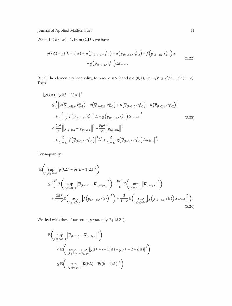
When 1 ≤ k ≤ M − 1, from (2.13), we have
y(kΔ) − y((k − 1)Δ) = u(y(k−1)Δ, r
Δk−1
)− u
(y(k−2)Δ, r
Δk−2
)+ f
(y(k−1)Δ, r
Δk−1
)Δ
+ g(y(k−1)Δ, r
Δk−1
)Δwk−1.
(3.22)
Recall the elementary inequality, for any x, y > 0 and ε ∈ (0, 1), (x + y)2 ≤ x2/ε + y2/(1 − ε).Then
∣∣y(kΔ) − y((k − 1)Δ)
∣∣2
≤ 1ε
∣∣∣u
(y(k−1)Δ, r
Δk−1
)− u
(y(k−2)Δ, r
Δk−1
)+ u
(y(k−2)Δ, r
Δk−1
)− u
(y(k−2)Δ, r
Δk−2
)∣∣∣
2
+1
1 − ε
∣∣∣f(y(k−1)Δ, r
Δk−1
)Δ + g
(y(k−1)Δ, r
Δk−1
)Δwk−1
∣∣∣2
≤ 2κ2
ε
∥∥∥y(k−1)Δ − y(k−2)Δ
∥∥∥2+
8κ2
ε
∥∥∥y(k−2)Δ
∥∥∥2
+2
1 − ε
∣∣∣f(y(k−1)Δ, r
Δk−1
)∣∣∣2Δ2 +
21 − ε
∣∣∣g(y(k−1)Δ, r
Δk−1
)Δwk−1
∣∣∣2.
(3.23)
Consequently
E
(
sup1≤k≤M−1
∣∣y(kΔ) − y((k − 1)Δ)∣∣2
)
≤ 2κ2
εE
(
sup1≤k≤M−1
∥∥∥y(k−1)Δ − y(k−2)Δ
∥∥∥2)
+8κ2
εE
(
sup1≤k≤M−1
∥∥∥y(k−2)Δ
∥∥∥2)
+2Δ2
1 − εE
(
sup1≤k≤M−1
∣∣∣f(y(k−1)Δ, r(t)
)∣∣∣
2)
+2
1 − εE
(
sup1≤k≤M−1
∣∣∣g(y(k−1)Δ, r(t)
)Δwk−1
∣∣∣2)
.
(3.24)
We deal with these four terms, separately. By (3.21),
E
(
sup1≤k≤M−1
∥∥∥y(k−1)Δ − y(k−2)Δ
∥∥∥2)
≤ E
(
sup1≤k≤M−1
sup−N≤i≤0
∣∣y((k + i − 1)Δ) − y((k − 2 + i)Δ)∣∣2
)
≤ E
(
sup−N≤k≤M−1
∣∣y(kΔ) − y((k − 1)Δ)∣∣2
)

12 Journal of Applied Mathematics
≤ E
(
sup−N≤k≤0
∣∣y(kΔ) − y((k − 1)Δ)
∣∣2
)
+ E
(
sup1≤k≤M−1
∣∣y(kΔ) − y((k − 1)Δ)
∣∣2
)
≤ α(Δ) + E
(
sup1≤k≤M−1
∣∣y(kΔ) − y((k − 1)Δ)
∣∣2
)
.
(3.25)
Noting that E[sup−τ≤t≤T |y(t)|2] ≤ E[sup−τ≤t≤T |y(t)|2] ≤ H(2) (where H(p) has been definedin Lemma 3.1), by Assumption 2.3 and (2.15),
E
(
sup1≤k≤M−1
∣∣∣f
(y(k−1)Δ, r
Δk−1
)∣∣∣
2)
≤ E
(
sup1≤k≤M−1
K
(1 +
∥∥∥y(k−1)Δ
∥∥∥2))
≤ K +KE
(
sup1≤k≤M−1
sup−N≤i≤0
∣∣y((k − 1 + i)Δ)∣∣2
)
≤ K +KE
(
sup−N≤k≤M−1
∣∣y(kΔ)∣∣2
)
≤ K +KE
(
sup−τ≤t≤T
∣∣y(t)∣∣2
)
≤ K(1 +H(2)).
(3.26)
By the Holder inequality, for any integer l > 1,
E
(
sup1≤k≤M−1
∣∣∣g(y(k−1)Δ, r
Δk−1
)Δwk−1
∣∣∣2)
≤ E
(
sup1≤k≤M−1
∣∣∣g(y(k−1)Δ, r(t)
)∣∣∣2
sup1≤k≤M−1
|Δwk−1|2)
≤[
E
(
sup1≤k≤M−1
∣∣∣g(y(k−1)Δ, r
Δk−1
)∣∣∣2l/(l−1)
)](l−1)/l[
E
(
sup1≤k≤M−1
|Δwk−1|2l)]1/l
≤[
E
(
sup0≤k≤M−1
(K
(1 +
∥∥ykΔ
∥∥2))l/(l−1)
)](l−1)/l[
E
(M−1∑
k=0
|Δwk|2l)]1/l
≤⎡
⎣Kl/(1−l)E
(
1 +
(
sup0≤k≤M−1
∥∥ykΔ
∥∥2
))l/(l−1)⎤
⎦
(l−1)/l[(M−1∑
k=0
E|Δwk|2l)]1/l

Journal of Applied Mathematics 13
≤[
21/(l−1)Kl/(1−l)(
1 + E
(
sup0≤k≤M−1
∥∥ykΔ
∥∥2l/(l−1)
))](l−1)/l[(M−1∑
k=0
(2l − 1)!!Δl
)]1/l
≤[
21/(l−1)Kl/(1−l)(
1 +H
(2l
l − 1
))](l−1)/l[(2l − 1)!!TΔl−1
]1/l
≤ D(l)Δ(l−1)/l,
(3.27)
where D(l) is a constant dependent on l.Substituting (3.25), (3.26), and (3.27) into (3.24), choosing ε = κ, and noting Δ ∈ (0, 1),
we have
E
(
sup1≤k≤M−1
∣∣y(kΔ) − y((k − 1)Δ)∣∣2
)
≤ 2κ1 − 2κ
α(Δ) +8κ
1 − 2κH(2) +
2K(1 +H(2)) + 2D(l)
(1 − 2κ)2Δ(l−1)/l.
(3.28)
Combining (3.21) with (3.28), from (3.20), we have
E
(
sup0≤k≤M−1
∥∥∥ykΔ − y(k−1)Δ
∥∥∥2)
≤ E
(
sup−N≤k≤M−1
∣∣y(kΔ) − y((k − 1)Δ)∣∣2
)
≤ E
(
sup−N≤k≤0
∣∣y(kΔ) − y((k − 1)Δ)∣∣2
)
+ E
(
sup1≤k≤M−1
∣∣y(kΔ) − y((k − 1)Δ)∣∣2
)
≤ 11 − 2κ
α(Δ) +8κ
1 − 2κH(2) +
2K(1 +H(2)) + 2D(l)
(1 − 2κ)2Δ(l−1)/l,
(3.29)
as required.
Lemma 3.3. If Assumptions 2.3–2.5 hold,
E
(
sup0≤s≤T
∥∥ys − ys
∥∥2
)
≤ c′2 + c2α(2Δ) + c2(l)Δ(l−1)/l =: β(Δ), (3.30)
where c2, c′2 are a constant independent of l andΔ, c2(l) is a constant dependent on l but independentof Δ.

14 Journal of Applied Mathematics
Proof. Fix any s ∈ [0, T] and θ ∈ [−τ, 0]. Let ks ∈ {0, 1, 2, . . . ,M−1}, kθ ∈ {−N,−N+1, . . . ,−1},and ksθ ∈ {−N,−N+1, . . . ,M−1} be the integers for which s ∈ [ksΔ, (ks+1)Δ], θ ∈ [kθΔ, (kθ+1)Δ], and s + θ ∈ [ksθΔ, (ksθ + 1)Δ], respectively. Clearly,
0 ≤ s + θ − (ks + kθ) ≤ 2Δ,
ksθ − (ks + kθ) ∈ {0, 1, 2}.(3.31)
From (2.7),
ys = yksΔ(θ)
= y((ks + kθ)Δ) +θ − kθΔ
Δ(y((ks + kθ + 1)Δ) − y(ks + kθ)Δ
),
(3.32)
which yields
∣∣ys − ys
∣∣ =∣∣∣y(s + θ) − yksΔ(θ)
∣∣∣
≤ ∣∣y(s + θ) − y((ks + kθ)Δ)∣∣ +
θ − kθΔΔ
∣∣y((ks + kθ + 1)Δ) − y((ks + kθ)Δ)∣∣
≤ ∣∣y(s + θ) − y((ks + kθ)Δ)∣∣ +
∣∣y((ks + kθ + 1)Δ) − y((ks + kθ)Δ)∣∣,
(3.33)
so by (3.20) and Lemma 3.2, noting y(MΔ) = y((M − 1)Δ) from (2.15),
E
(
sup0≤s≤T
∥∥ys − ys
∥∥2
)
≤ 2E
[
sup0≤s≤T
(
sup−τ≤θ≤0
∣∣y(s + θ) − y((ks + kθ)Δ)∣∣2
)]
+ 2E
[
sup0≤ks≤M−1
(
sup−N≤kθ≤0
∣∣y((ks + kθ + 1)Δ) − y((ks + kθ)Δ)∣∣2
)]
≤ 2E
(
sup−τ≤θ≤0,0≤s≤T
∣∣y(s + θ) − y((ks + kθ)Δ)∣∣2
)
+ 2γ(Δ).
(3.34)
Therefore, it is a key to compute E(sup−τ≤θ≤0,0≤s≤T |y(s + θ) − y((ks + kθ)Δ)|2). We discuss thefollowing four possible cases.
Case 1 (ks + kθ ≥ 0). We again divide this case into three possible subcases according toksθ − (ks + kθ) ∈ {0, 1, 2}.

Journal of Applied Mathematics 15
Subcase 1 (ksθ − (ks + kθ) = 0). From (2.13),
y(s + θ) − y((ks + kθ)Δ) = u
(y(ksθ−1) Δ +
s + θ − ksθΔΔ
(yksθΔ − y(ksθ−1)Δ
), rΔksθ
)
− u(y(ksθ−1)Δ, r
Δksθ−1
)+∫ s+θ
ksθΔf(yv, r(v)
)dv
+∫s+θ
ksθΔg(yv, r(v)
)dw(v),
(3.35)
which yields
E
(
sup−τ≤θ≤0,0≤s≤T,ks+kθ≥0
∣∣y(s + θ) − y((ks + kθ)Δ)∣∣2
)
≤ 3E
(
sup−τ≤θ≤0,0≤s≤T,ksθ≥0
∣∣∣∣u(y(ksθ−1)Δ +
s + θ − ksθΔΔ
(yksθΔ − y(ksθ−1)Δ, r
Δksθ
))
−u(y(ksθ−1)Δ, r
Δksθ−1
)∣∣∣∣
2)
+ 3E
⎛
⎝ sup−τ≤θ≤0,0≤s≤T,ksθ≥0
∣∣∣∣∣
∫ s+θ
ksθΔf(yr, r(r)
)dr
∣∣∣∣∣
2⎞
⎠
+ 3E
⎛
⎝ sup−τ≤θ≤0,0≤s≤T,ksθ≥0
∣∣∣∣∣
∫s+θ
ksθΔg(yr, r(r)
)dw(r)
∣∣∣∣∣
2⎞
⎠.
(3.36)
From Assumption 2.4, (3.24), (3.26), and Lemma 3.2, we have
E
(
sup−τ≤θ≤0,0≤s≤T,ksθ≥0
∣∣∣∣u(y(ksθ−1)Δ+
s+θ−ksθΔΔ
(yksθΔ−y(ksθ−1)Δ, r
Δksθ
))−u
(y(ksθ−1)Δ, r
Δksθ−1
)∣∣∣∣
2)
≤ 2κ2E
(
sup−τ≤θ≤0,0≤s≤T,ksθ≥0
∥∥∥∥s + θ − ksθΔ
Δ
(yksθΔ − y(ksθ−1)Δ
)∥∥∥∥
2)
+ 8κ2H(2)
≤ 2κ2E
(
sup−τ≤θ≤0,0≤s≤T,ksθ≥0
∥∥∥(yksθΔ − y(ksθ−1)Δ
)∥∥∥2)
+ 8κ2H(2)
≤ 2κ2E
(
sup0≤ksθ≤M−1
∥∥∥(yksθΔ − y(ksθ−1)Δ
)∥∥∥2)
+ 8κ2H(2)
≤ 2κ2γ(Δ) + 8κ2H(2).(3.37)

16 Journal of Applied Mathematics
By the Holder inequality, Assumption 2.3, and Lemma 3.1,
E
⎛
⎝ sup−τ≤θ≤0,0≤s≤T,ksθ≥0
∣∣∣∣∣
∫s+θ
ksθΔf(yr, r(r)
)dr
∣∣∣∣∣
2⎞
⎠
≤ ΔE
(
sup−τ≤θ≤0,0≤s≤T,ksθ≥0
∫s+θ
ksθΔ
∣∣f
(yr, r(r)
)∣∣2dr
)
≤ KΔE
(
sup−τ≤θ≤0,0≤s≤T,ksθ≥0
∫s+θ
ksθΔ
(1 +
∥∥yr
∥∥2
)dr
)
≤ KΔE
[∫T
0
(
1 + sup0≤r≤T
∥∥yr
∥∥2
)
dr
]
≤ KΔ∫T
0
[
1 + E
(
sup−τ≤t≤T
y(t)|2)]
dr
≤ KΔ∫T
0[1 +H(2)]dr
≤ KT[1 +H(2)]Δ.
(3.38)
Setting v = s + θ and kv = ksθ and applying the Holder inequality yield
E
⎛
⎝ sup−τ≤θ≤0,0≤s≤T,ksθ≥0
∣∣∣∣∣
∫s+θ
ksθΔg(yr, r(r)
)dw(r)
∣∣∣∣∣
2⎞
⎠
= E
(
sup0≤v≤T,0≤kv≤M−1
∣∣∣g(ykvΔ, r(v)
)(w(v) −w(kvΔ))
∣∣∣2)
≤[
E
(
sup0≤v≤T,0≤kv≤M−1
∣∣∣g(ykvΔ, r(v)
)∣∣∣2l/(l−1)
)](l−1)/l
×[
E
(
sup0≤v≤T,0≤kv≤M−1
|w(v) −w(kvΔ)|2l)]1/l
.
(3.39)
The Doob martingale inequality gives
E
(
sup0≤v≤T,0≤kv≤M−1
|w(v) −w(kvΔ)|2l)
= E
(
sup0≤kv≤M−1
(
supkvΔ≤v≤(kv+1)Δ
|w(v) −w(kvΔ)|2l))

Journal of Applied Mathematics 17
≤ E
(M−1∑
kv=0
(
supkvΔ≤v≤(kv+1)Δ
|w(v) −w(kvΔ)|2l))
=M−1∑
kv=0
E
(
supkvΔ≤v≤(kv+1)Δ
|w(v) −w(kvΔ)|2l)
≤(
2l2l − 1
)2l M−1∑
kv=0
E|w((kv + 1)Δ) −w(kvΔ)|2l.
(3.40)
By (3.27), we therefore have
E
⎛
⎝ sup−τ≤θ≤0,0≤s≤T,ksθ≥0
∣∣∣∣∣
∫ s+θ
ksθΔg(yr, r(r)
)dw(r)
∣∣∣∣∣
2⎞
⎠
≤(
2l2l − 1
)2[
E
(
sup0≤kv≤M−1
∣∣∣g(ykvΔ, r(v)
)∣∣∣2l/(l−1)
)](l−1)/l
×[M−1∑
kv=0
E|w((kv + 1)Δ) −w(kvΔ)|2l]1/l
≤(
2l2l − 1
)2
D(l)Δ(l−1)/l.
(3.41)
Substituting (3.37), (3.38), and (3.41) into (3.36) and noting Δ ∈ (0, 1) give
E
(
sup−τ≤θ≤0,0≤s≤T,ks+kθ≥0
∣∣y(s + θ) − y((ks + kθ)Δ)∣∣2
)
≤ 6κ2γ(Δ) + 24κ2H(2) + 3
(
KT(1 +H(2)) +(
2l2l − 1
)2
D(l)
)
Δ(l−1)/l
=: 6κ2γ(Δ) + 24κ2H(2) + c1(l)Δ(l−1)/l.
(3.42)
Subcase2 (ksθ − (ks + kθ) = 1). From (2.13),
y(s + θ) − y((ks + kθ)Δ) = y(ksθΔ) − y((ks + kθ)Δ) + y(s + θ) − y(ksθΔ)
≤ u(y(ks+kθ)Δ, r
Δks+kθ
)− u
(y(ks+kθ−1)Δ, r
Δks+kθ−1
)+ f
(y(ks+kθ)Δ, r
Δks+kθ
)Δ
+ g(y(ks+kθ)Δ, r
Δks+kθ
)Δwks+kθ + y(s + θ) − y(ksθΔ),
(3.43)

18 Journal of Applied Mathematics
so we have
E
(
sup−τ≤θ≤0,0≤s≤T,ks+kθ≥0
∣∣y(s + θ) − y((ks + kθ)Δ)
∣∣2
)
≤ 4
{
E
(
sup−τ≤θ≤0,0≤s≤T,ks+kθ≥0
∣∣∣u
(y(ks+kθ)Δ, r
Δks+kθ
)− u
(y(ks+kθ−1)Δ, r
Δks+kθ−1
)∣∣∣
2)
+ E
(
sup−τ≤θ≤0,0≤s≤T,ks+kθ≥0
∣∣∣f
(y(ks+kθ)Δ, r
Δks+kθ
)Δ∣∣∣
2)
+ E
(
sup−τ≤θ≤0,0≤s≤T,ks+kθ≥0
∣∣∣g
(y(ks+kθ)Δ, r
Δks+kθ
)Δwks+kθ
∣∣∣
2)
+E
(
sup−τ≤θ≤0,0≤s≤T,ks+kθ≥0
∣∣y(s + θ) − y(ksθΔ)∣∣2
)}
.
(3.44)
Since
E
(
sup−τ≤θ≤0,0≤s≤T,ks+kθ≥0
∣∣∣u(y(ks+kθ)Δ, r
Δks+kθ
)− u
(y(ks+kθ−1)Δ, r
Δks+kθ−1
)∣∣∣2)
≤ 2κ2γ(Δ) + 8κ2H(2),
(3.45)
from (3.26), (3.27), and the Subcase 1, noting Δ ∈ (0, 1), we have
E
(
sup−τ≤θ≤0,0≤s≤T,ks+kθ≥0
∣∣y(s + θ) − y((ks + kθ)Δ)∣∣2
)
≤ 4{
2κ2γ(Δ) + 8κ2H(2) +K[1 +H(2)]Δ2 +D(l)Δ(l−1)/l
+3(
2κ2γ(Δ) + 8κ2H(2))(Δ) + c1(l)Δ(l−1)/l
}
=: 32κ2γ(Δ) + 128κ2H(2) + c2(l)Δ(l−1)/l.
(3.46)
Subcase 3 (ksθ − (ks + kθ) = 2). From (2.13), we have
y(s + θ) − y((ks + kθ)Δ) = y(s + θ) − y((ksθ − 1)Δ) + y((ksθ − 1)Δ) − y((ks + kθ)Δ),(3.47)

Journal of Applied Mathematics 19
so from the Subcase 2, we have
E
(
sup−τ≤θ≤0,0≤s≤T,ks+kθ≥0
∣∣y(s + θ) − y((ks + kθ)Δ)
∣∣2
)
≤ 2E
(
sup−τ≤θ≤0,0≤s≤T,ks+kθ≥0
∣∣y(s + θ) − y((ksθ − 1)Δ)
∣∣2
)
+ 2E
(
sup−τ≤θ≤0,0≤s≤T,ks+kθ≥0
∣∣y((ksθ − 1)Δ) − y((ks + kθ)Δ)
∣∣2
)
≤ 2[32κ2γ(Δ) + 128κ2H(2) + c2(l)Δ(l−1)/l
]
+ 2[2κ2γ(Δ) + 8κ2H(2) +K[1 +H(2)]Δ2 +D(l)Δ(l−1)/l
]
=: 68κ2γ(Δ) + 272κ2H(2) + c3(l)Δ(l−1)/l.
(3.48)
From these three subcases, we have
E
(
sup−τ≤θ≤0,0≤s≤T,ks+kθ≥0
∣∣y(s + θ) − y((ks + kθ)Δ)∣∣2
)
≤ 106κ2γ(Δ) + 424κ2H(2) + [c1(l) + c2(l) + c3(l)]Δ(l−1)/l.
(3.49)
Case 2 (ks + kθ = −1 and 0 ≤ s + θ ≤ Δ). In this case, applying Assumption 2.5 and case 1, wehave
E
(
sup−τ≤θ≤0,0≤s≤T
∣∣y(s + θ) − y((ks + kθ)Δ)∣∣2
)
≤ 2E
(
sup−τ≤θ≤0,0≤s≤T
∣∣y(s + θ) − y(0)∣∣2
)
+ 2E∣∣y(0) − y(−Δ)
∣∣2
≤ 212κ2γ(Δ) + 848κ2H(2) + 2[c1(l) + c2(l) + c3(l)]Δ(l−1)/l + 2α(Δ).
(3.50)
Case 3 (ks + kθ = −1 and −Δ ≤ s + θ ≤ 0). In this case, using Assumption 2.5,
E
(
sup−τ≤θ≤0,0≤s≤T
∣∣y(s + θ) − y((ks + kθ)Δ)∣∣2
)
≤ α(Δ). (3.51)

20 Journal of Applied Mathematics
Case 4 (ks + kθ ≤ −2). In this case, s + θ ≤ 0, so using Assumption 2.5,
E
(
sup−τ≤θ≤0,0≤s≤T
∣∣y(s + θ) − y((ks + kθ)Δ)
∣∣2
)
≤ α(2Δ). (3.52)
Substituting these four cases into (3.34) and noting the expression of γ(Δ), there exist c2, c′2,and c2(l) such that
E
(
sup0≤s≤T
∥∥ys − ys
∥∥2
)
≤ c2α(2Δ) + c′2 + c2(l)Δ(l−1)/l, (3.53)
This proof is complete.
Remark 3.4. It should be pointed out that much simpler proofs of Lemmas 3.2 and 3.3 can beobtained by choosing l = 2 if we only want to prove Theorem 2.7. However, here we choosel > 1 to control the stochastic terms β(Δ) and γ(Δ) by Δ(l−1)/l in Section 3, which will be usedto show the order of the strong convergence.
Lemma 3.5. If Assumption 2.4 holds,
E
(
sup0≤t≤T
∣∣u(yt, r(t)
) − u(yt, r(t)
)∣∣2
)
≤ 8κ2H(2)LΔ := ζΔ (3.54)
where L is a positive constant independent of Δ.
Proof. Let n = [T/Δ], the integer part of T/Δ, and 1G be the indication function of the set G.Then, by Assumption 2.4 and Lemma 3.1, we obtain
E
(
sup0≤t≤T
∣∣u(yt, r(t)
) − u(yt, r(t)
)∣∣2
)
≤ max0≤k≤n
E
(
sups∈[tk ,tk+1)
∣∣u(ys, r(s)
) − u(ys, r(s)
)∣∣2
)
≤ 2max0≤k≤n
E
(
sups∈[tk ,tk+1)
∣∣u(ys, r(s)
) − u(ys, r(s)
)∣∣21{r(s)/= r(tk)}
)
≤ 4max0≤k≤n
E
(
sups∈[tk ,tk+1)
(|u(ys, r(s))|2 +
∣∣u(ys, r(s)
)∣∣2)
1{r(s)/= r(tk)}
)
≤ 8κ2 max0≤k≤n
(
E
(
sup0≤t≤T
∥∥yt
∥∥2
))
E(1{r(s)/= r(tk)}
)

Journal of Applied Mathematics 21
≤ 8κ2H(2)E(1{r(s)/= r(tk)}
)
= 8κ2H(2)E[E(1{r(s)/= r(tk)} | (tk)
)],
(3.55)
where in the last step we use the fact that ytkand 1{r(s)/= r(tk)} are conditionally independent
with respect to the σ− algebra generated by r(tk). But, by the Markov property,
E(1{r(s)/= r(tk)} | r(tk)
)=
∑
i∈S1{r(tk)=i}P(r(s)/= i | r(tk) = i)
=∑
i∈S1{r(tk)=i}
∑
j /= i
(γij(s − tk) + o(s − tk)
)
≤∑
i∈S1{r(tk)=i}
(max1≤i≤N
(−γij)Δ + o(Δ)
)
≤ LΔ,
(3.56)
where L is a positive constant independent of Δ. Then
E
(
sup0≤t≤T
∣∣u(yt, r(t)
) − u(yt, r(t)
)∣∣2
)
≤ 8κ2H(2)LΔ. (3.57)
This proof is complete.
Lemma 3.6. If Assumption 2.3 holds, there is a constant C, which is independent of Δ such that
E
∫T
0
∣∣f(ys, r(s)
) − f(ys, r(s)
)∣∣2ds ≤ CΔ, (3.58)
E
∫T
0
∣∣g(ys, r(s)
) − g(ys, r(s)
)∣∣2ds ≤ CΔ. (3.59)
Proof. Let n = [T/Δ], the integer part of T/Δ. Then
E
∫T
0
∣∣f(ys, r(s)
) − f(ys, r(s)
)∣∣2ds =
n∑
k=0
E
∫ tk+1
tk
∣∣∣f(ytk
, r(s))− f
(ytk
, r(tk))∣∣∣
2ds, (3.60)

22 Journal of Applied Mathematics
with tn+1 being T . Let 1G be the indication function of the set G. Moreover, in what follows,C is a generic positive constant independent of Δ, whose values may vary from line to line.With these notations we derive, using Assumption 2.3, that
E
∫ tk+1
tk
∣∣∣f
(ytk
, r(s))− f
(ytk
, r(tk))∣∣∣
2ds
≤ 2E
∫ tk+1
tk
[|f(ytk
, r(s))|2 +∣∣∣f
(ytk
, r(tk))∣∣∣
2]
1{r(s)/= r(tk)}ds
≤ CE
∫ tk+1
tk
(1 +
∥∥∥ytk
∥∥∥
2)
1{r(s)/= r(tk)}ds
≤ C
∫ tk+1
tk
E
[E
[(1 +
∥∥∥ytk
∥∥∥
2)
1{r(s)/= r(tk)} | r(tk)]]
ds
≤ C
∫ tk+1
tk
E
[E
[(1 +
∥∥∥ytk
∥∥∥2)
| r(tk)]E[1{r(s)/= r(tk)} | r(tk)
]]ds,
(3.61)
where in the last step we use the fact that ytkand 1{r(s)/= r(tk)} are conditionally independent
with respect to the σ− algebra generated by r(tk). But, by the Markov property,
E[1{r(s)/= r(tk)} | r(tk)
]=
∑
i∈S1{r(tk)=i}P(r(s)/= i | r(tk) = i)
=∑
i∈S1{r(tk)=i}
∑
j /= i
(γij(s − tk) + o(s − tk)
)
≤∑
i∈S1{r(tk)=i}
(max1≤i≤N
(−γij)Δ + o(Δ)
)
≤ CΔ.
(3.62)
So, by Lemma 3.1,
E
∫ tk+1
tk
∣∣∣f(ytk
, r(s))− f
(ytk
, r(tk))∣∣∣
2ds ≤ CΔ
∫ tk+1
tk
(1 + E
∥∥∥ytk
∥∥∥2)ds
≤ CΔ2.
(3.63)
Therefore
E
∫T
0
∣∣f(ys, r(s)
) − f(ys, r(s)
)∣∣2ds ≤ CΔ. (3.64)
Similarly, we can show (3.59).

Journal of Applied Mathematics 23
4. Convergence of the EM Methods
In this section we will use the lemmas above to prove Theorem 2.7. From Lemma 3.1 andTheorem 2.6, there exists a positive constant H such that
E
(
sup−τ≤t≤T
|x(t)|p)
∨ E
(
sup−τ≤t≤T
∣∣y(t)
∣∣p)
≤ H. (4.1)
Let j be a sufficient large integer. Define the stopping times
uj := inf{t ≥ 0 : ‖xt‖ ≥ j
}, vj := inf
{t ≥ 0 :
∥∥yt
∥∥ ≥ j
}, ρj := uj ∧ vj , (4.2)
where we set inf ∅ = ∞ as usual. Let
e(t) := x(t) − y(t). (4.3)
Obviously,
E
(
sup0≤t≤T
|e(t)|2)
= E
(
sup0≤t≤T
|e(t)|21{uj>T,vj>T}
)
+ E
(
sup0≤t≤T
|e(t)|21{uj≤T or vj≤T}
)
. (4.4)
Recall the following elementary inequality:
aγb1−γ ≤ γa +(1 − γ
)b, ∀a, b > 0, γ ∈ [0, 1]. (4.5)
We thus have, for any δ > 0,
E
(
sup0≤t≤T
|e(t)|21{uj≤Tor vj≤T}
)
≤ E
⎡
⎣
(
δ sup{0≤t≤T}
|e(t)|p)2/p(
δ−2/(p−2)1{uj≤T or vj≤T})(p−2)/p
⎤
⎦
≤ 2δp
E
(
sup0≤t≤T
|e(t)|p)
+p − 2
pδ2/(p−2)P(uj ≤ Tor vj ≤ T
).
(4.6)
Hence
E
(
sup0≤t≤T
|e(t)|2)
≤ E
(
sup0≤t≤T
|e(t)|21{ρj>T}
)
+2δp
E
(
sup0≤t≤T
|e(t)|p)
+p − 2
pδ2/(p−2)P(uj ≤ T or vj ≤ T
).
(4.7)

24 Journal of Applied Mathematics
Now,
P(uj ≤ T
) ≤ E
(1{uj≤T}
‖xt‖pjp
)
≤ 1jp
E
(
sup−τ≤t≤T
|x(t)|p)
≤ H
jp.
(4.8)
Similarly,
P(vj ≤ T
) ≤ H
jp. (4.9)
Thus
P(vj ≤ T or uj ≤ T
) ≤ P(vj ≤ T
)+ P
(uj ≤ T
)
≤ 2Hjp
.(4.10)
We also have
E
(
sup0≤t≤T
|e(t)|p)
≤ 2p−1E
(
sup0≤t≤T
(|xt|p +∣∣yt
∣∣p))
≤ 2pH.
(4.11)
Moreover,
E
(
sup0≤t≤T
|e(t)|21{ρj>T}
)
= E
(
sup0≤t≤T
∣∣e(t ∧ ρj
)∣∣21{ρj>T}
)
≤ E
(
sup0≤t≤T
∣∣e(t ∧ ρj
)∣∣2
)
.
(4.12)
Using these bounds in (4.7) yields
E
(
sup0≤t≤T
|e(t)|2)
≤ E
(
sup0≤t≤T
∣∣e(t ∧ ρj
)∣∣2
)
+2p+1δH
p+
2(p − 2
)H
pδ2/(p−2) jp. (4.13)

Journal of Applied Mathematics 25
Setting v := t ∧ ρj and for any ε ∈ (0, 1), by the Holder inequality, when v ∈ [kΔ, (k + 1)Δ],for k = 0, 1, 2, . . . ,M − 1,
|e(v)|2 =∣∣x(v) − y(v)
∣∣2
≤∣∣∣∣u(xv, r(v)) − u
(y(k−1)Δ +
(v − kΔ)Δ
(ykΔ − y(k−1)Δ
), rΔk
)
+∫v
0
[f(xs, r(s)) − f
(ys, r(s)
)]ds +
∫v
0
[g(xs, r(s)) − g
(ys, r(s)
)]dw(s)
∣∣∣∣
2
≤ 1ε
∣∣∣∣u(xv, r(v)) − u
(y(k−1)Δ +
(v − kΔ)Δ
(ykΔ − y(k−1)Δ
), rΔk
)∣∣∣∣
2
+2
1 − ε
[
T
∫v
0
[f(xs, r(s))−f
(ys, r(s)
)]2ds+
∣∣∣∣
∫v
0
[g(xs, r(s))−g
(ys, r(s)
)]dw(s)
∣∣∣∣
2]
.
(4.14)
Assumption 2.4 yields
∣∣∣∣u(xv, r(v)) − u
(y(k−1)Δ +
v − kΔΔ
(ykΔ − y(k−1)Δ
), rΔk
)∣∣∣∣
2
≤ 2κ2∥∥∥∥xv − y(k−1)Δ − v − kΔ
Δ
(ykΔ − y(k−1)Δ
)∥∥∥∥
2
+ 2∣∣∣∣u
(y(k−1)Δ +
v − kΔΔ
(ykΔ − y(k−1)Δ
), r(v)
)
−u(y(k−1)Δ +
v − kΔΔ
(ykΔ − y(k−1)Δ
), rΔk
)∣∣∣∣
2
≤ 2κ2∥∥∥∥∣∣xv − yv
∣∣ +∣∣yv − yv
∣∣ +∣∣∣ykΔ − y(k−1)Δ
∣∣∣ − v − kΔΔ
∣∣∣ykΔ − y(k−1)Δ
∣∣∣∥∥∥∥
2
+ 2∣∣∣∣u
(y(k−1)Δ +
v − kΔΔ
(ykΔ − y(k−1)Δ
), r(v)
)
−u(y(k−1)Δ +
v − kΔΔ
(ykΔ − y(k−1)Δ
), rΔk
)∣∣∣∣
2
≤ 2κ2
ε
∥∥xv − yv
∥∥2 +4κ2
1 − ε
(∥∥yv − yv
∥∥2 +∥∥∥ykΔ − y(k−1)Δ
∥∥∥2)
+ 2∣∣∣∣u
(y(k−1)Δ +
v − kΔΔ
(ykΔ − y(k−1)Δ
), r(v)
)
−u(y(k−1)Δ +v − kΔ
Δ(ykΔ − y(k−1)Δ), r
Δk )
∣∣∣∣
2
.
(4.15)

26 Journal of Applied Mathematics
Then, we have
|e(v)|2 ≤ 2κ2
ε2
∥∥xv − yv
∥∥2 +
4κ2
ε(1 − ε)
(∥∥yv − yv
∥∥2 +
∥∥∥ykΔ − y(k−1)Δ
∥∥∥
2)
+ 2∣∣∣∣u
(y(k−1)Δ +
v − kΔΔ
(ykΔ − y(k−1)Δ
), r(v)
)
−u(y(k−1)Δ +
v − kΔΔ
(ykΔ − y(k−1)Δ
), rΔk
)∣∣∣∣
2
+2
1 − ε
[
T
∫v
0
[f(xs, r(s))−f
(ys, r(s)
)]2ds+
∣∣∣∣
∫v
0
[g(xs, r(s))−g
(ys, r(s)
)]dw(s)
∣∣∣∣
2]
.
(4.16)
Hence, for any t1 ∈ [0, T], by Lemmas 3.2–3.5,
E
[
sup0≤t≤t1
∣∣e(t ∧ ρj
)∣∣2
]
≤ 2κ2
ε2E
(
sup0≤t≤t1
∥∥∥xt∧ρj − yt∧ρj∥∥∥
2)
+4κ2
ε(1 − ε)
[
E
(
sup0≤t≤t1
∥∥∥yt∧ρj − yt∧ρj
∥∥∥2)
+E
(
sup0≤k≤M−1
∥∥∥ykΔ∧ρj − y(k−1)Δ∧ρj
∥∥∥2)]
+2E
[
sup0≤k≤M−1
∣∣∣∣∣u
(
y(k−1)Δ+kΔ ∧ ρj − kΔ
Δ
(ykΔ−y(k−1)Δ
), r
(kΔ ∧ ρj
))
−u(
y(k−1)Δ +kΔ ∧ ρj − kΔ
Δ
(ykΔ − y(k−1)Δ
), r
(kΔ ∧ ρj
))∣∣∣∣∣
2⎤
⎦
+2T
1 − εE
∫ t1∧ρj
0
[f(xs, r(s)) − f
(ys
), r(s)
]2ds
+2
1 − εE
⎡
⎣ sup0≤t≤t1
∣∣∣∣∣
∫ t∧ρj
0
[g(xs, r(s)) − g
(ys, r(s)
)]dw(s)
∣∣∣∣∣
2⎤
⎦
≤ 2κ2
ε2E
(
sup0≤t≤t1
∥∥∥xt∧ρj − yt∧ρj∥∥∥
2)
+4κ2
ε(1 − ε)(γ(Δ) + β(Δ)
)+ 2ζΔ
+2T
1 − εE
∫ t1∧ρj
0
[f(xs, r(s)) − f
(ys, r(s)
)]2ds
+2
1 − εE
⎡
⎣ sup0≤t≤t1
∣∣∣∣∣
∫ t∧ρj
0
[g(xs, r(s)) − g
(ys, r(s)
)]dw(s)
∣∣∣∣∣
2⎤
⎦.
(4.17)

Journal of Applied Mathematics 27
Since x(t) = y(t) = ξ(t) when t ∈ [−τ, 0], we have
E
(
sup0≤t≤t1
∥∥∥xt∧ρj − yt∧ρj
∥∥∥
2)
≤ E
(
sup−τ≤θ≤0
sup0≤t≤t1
∣∣x
(t ∧ ρj + θ
) − y(t ∧ ρj + θ
)∣∣2
)
≤ E
(
sup−τ≤t≤t1
∣∣x
(t ∧ ρj
) − y(t ∧ ρj
)∣∣2
)
= E
(
sup0≤t≤t1
∣∣x
(t ∧ ρj
) − y(t ∧ ρj
)∣∣2
)
.
(4.18)
By Assumption 2.2, Lemma 3.3, and Lemma 3.6, we may compute
E
∫ t1∧ρj
0
∣∣f(xs, r(s)) − f(ys, r(s)
)∣∣2ds
≤ E
∫ t1∧ρj
0
∣∣f(xs, r(s)) − f(ys, r(s)
)+ f
(ys, r(s)
) − f(ys, r(s)
)∣∣2ds
≤ 2CjE
∫ t1∧ρj
0
∥∥xs − ys + ys − ys
∥∥2ds + 2CΔ
≤ 4CjE
∫ t1∧ρj
0
∥∥xs − ys
∥∥2ds + 4CjE
∫ t1∧ρj
0
∥∥ys − ys
∥∥2ds + 2CΔ
≤ 4CjE
∫ t1∧ρj
0sup
−τ≤θ≤0
∣∣x(s + θ) − y(s + θ)∣∣2ds + 4CjTβ(Δ) + 2CΔ
≤ 4CjE
∫ t1
0sup
−τ≤θ≤0
∣∣x(s ∧ ρj + θ
) − y(s ∧ ρj + θ
)∣∣2ds
+ 4CjTβ(Δ) + 2CΔ
≤ 4CjE
∫ t1
0sup
−τ≤r≤s
∣∣x(r ∧ ρj
) − y(r ∧ ρj
)∣∣2ds + 4CjTβ(Δ) + 2CΔ
= 4Cj
∫ t1
0Esup
0≤r≤s
∣∣x(r ∧ ρj
) − y(r ∧ ρj
)∣∣2ds + 4CjTβ(Δ) + 2CΔ.
(4.19)
By the Doob martingale inequality, Lemma 3.3, Lemma 3.6, and Assumption 2.2, we compute
E
⎡
⎣ sup0≤t≤t1
∣∣∣∣∣
∫ t∧ρj
0
[g(xs, r(s)) − g
(ys, r(s)
)]dw(s)
∣∣∣∣∣
2⎤
⎦
= E
⎡
⎣ sup0≤t≤t1
∣∣∣∣∣
∫ t∧ρj
0
[g(xs, r(s)) − g
(ys, r(s)
)+ g
(ys, r(s)
) − g(ys, r(s)
)]dw(s)
∣∣∣∣∣
2⎤
⎦

28 Journal of Applied Mathematics
≤ 8CjE
∫ t1∧ρj
0
∥∥xs − ys
∥∥2ds + 8CΔ
≤ 16Cj
∫ t1
0E
(
sup0≤r≤s
∣∣x
(r ∧ ρj
) − y(r ∧ ρj
)∣∣2
)
ds + 16CjTβ(Δ) + 8CΔ.
(4.20)
Therefore, (4.17) can be written as
(
1 − 2κ2
ε2
)
E
[
sup0≤t≤t1
∣∣e
(t ∧ ρj
)∣∣2
]
≤ 4κ2
ε(1 − ε)[β(Δ) + γ(Δ)
]+
8CjT(T + 4)1 − ε
β(Δ) +4CΔ(T + 8)
1 − ε
+ 2ζΔ +8Cj(T + 4)
1 − ε
∫ t1
0E
(
sup0≤v≤s
∣∣e(v ∧ ρj
)∣∣2
)
ds.
(4.21)
Choosing ε = (1 +√
2κ)/2 and noting κ ∈ (0, 1), we have
E
(
sup0≤t≤t1
∣∣e(t ∧ ρj
)∣∣2
)
≤16κ2
(1 +
√2κ
)
(1 − √
2κ)2(
1 + 3√
2κ)[β(Δ) + γ(Δ)
]+
16CjT(
1 +√
2κ)2(T + 4)
(1 − √
2κ)2(
1 + 3√
2κ) β(Δ)
+8CΔ(T + 8)
(1 +
√2κ
)2
(1 − √
2κ)2(
1 + 3√
2κ) +
2(
1 +√
2κ)2
(1 − √
2κ)2(
1 + 3√
2κ)ζΔ
+16Cj
(1 +
√2κ
)2(T + 4)
(1 − √
2κ)2(
1 + 3√
2κ)
∫ t1
0E
(
sup0≤s≤v
∣∣e(s ∧ ρj
)∣∣2
)
dv
≤ 16(
1 − √2κ
)2
[β(Δ) + γ(Δ)
]+
16CjT(T + 4)(
1 − √2κ
)2β(Δ) +
8CΔ(T + 8)(
1 − √2κ
)2
+2
(1 − √
2κ)ζΔ +
16Cj(T + 4)(
1 − √2κ
)2
∫ t1
0E
(
sup0≤s≤v
∣∣e(s ∧ ρj
)∣∣2
)
dv.
(4.22)

Journal of Applied Mathematics 29
By the Gronwall inequality, we have
E
[
sup0≤t≤t1
∣∣e
(t ∧ ρj
)∣∣2
]
≤
⎡
⎢⎣
16
(1 − √2κ)
2
(β(Δ) + γ(Δ)
)+
16CjT(T + 4)(
1 − √2κ
)2β(Δ)
+8CΔ(T + 8)(
1 − √2κ
)2+
2ζΔ(
1 − √2κ
)
⎤
⎥⎦ × e(16/(1−√2κ)2)CjT(T+4).
(4.23)
By (4.13),
E
(
sup0≤t≤T
|e(t)|2)
≤
⎡
⎢⎣
16(
1 − √2κ
)2
(β(Δ) + γ(Δ)
)+
16CjT(T + 4)(
1 − √2κ
)2β(Δ) +
8CΔ(T + 8)(
1 − √2κ
)2
+2ζΔ
(1 − √
2κ)
⎤
⎥⎦ × e(16/(1−√2κ)2)CjT(T+4) +
2p+1δH
p+
2(p − 2
)H
pδ2/(p−2)jp.
(4.24)
Given any ε > 0, we can now choose δ sufficient small such that 2p+1δH/p ≤ ε/3, then choosej sufficient large such that
2(p − 2
)H
pδ2/(p−2)jp<
ε
3, (4.25)
and finally choose Δ so small such that
⎡
⎢⎣
16(
1 − √2κ
)2
(β(Δ) + γ(Δ)
)+
16CjT(T + 4)(
1 − √2κ
)2β(Δ) +
8CΔ(T + 8)(
1 − √2κ
)2+
2ζΔ(
1 − √2κ
)
⎤
⎥⎦
× e(16/(1−√2κ)2)CjT(T+4) <
ε
3
(4.26)
and thus E(sup0≤t≤T |e(t)|2) ≤ ε as required.
Remark 4.1. Obviously, according to Theorem 2.7, for neutral stochastic delay differentialequations with Markovian switching [19], we can easily obtain that the numerical solutionsconverge to the true solutions in mean square under Assumptions 2.2–2.4.
5. Convergence Order of the EM Method
To reveal the convergence order of the EM method, we need the following assumptions.

30 Journal of Applied Mathematics
Assumption 5.1. There exists a constant Q such that for all ϕ, ψ ∈ C([−τ, 0]; Rn), i ∈ S, andt ∈ [0, T],
∣∣f
(ϕ, i
) − f(ψ, i
)∣∣2 ∨ ∣∣g
(ϕ, i
) − g(ψ, i
)∣∣2 ≤ Q∥∥ϕ − ψ
∥∥2
. (5.1)
It is easy to see from the global Lipschitz condition that, for any ϕ ∈ C([−τ, 0]; Rn),
∣∣f
(ϕ, i
)∣∣2 ∨ ∣∣g
(ψ, i
)∣∣2 ≤ 2(∣∣f(0, i)
∣∣2 ∨ ∣
∣g(0, i)∣∣2)+Q
∥∥ϕ
∥∥2
. (5.2)
In other words, the global Lipschitz condition implies linear growth condition with thegrowth coefficient
K = 2[∣∣f(0, i)
∣∣2 ∨ ∣∣g(0, i)∣∣2 ∨Q
]. (5.3)
Assumption 5.2. ξ ∈ Lp
F0([−τ, 0]; Rn) for some p ≥ 2, and there exists a positive constant λ such
that
E
(
sup−τ≤s≤t≤0
|ξ(t) − ξ(s)|2)
≤ λ(t − s). (5.4)
We can state another theorem, which reveals the order of the convergence.
Theorem 5.3. If Assumptions 5.1, 5.2, and 2.4 hold, for any positive constant l > 1,
E
(
sup0≤t≤T
∣∣x(t) − y(t)∣∣2
)
≤ O(Δ1−1/l
). (5.5)
Proof. Since α(Δ) may be replaced by λΔ, from Lemmas 3.2 and 3.3, there exist constants c1(l)and c2(l) such that β(Δ) ≤ c1(l)Δ(l−1)/l and γ(Δ) ≤ c2(l)Δ(l−1)/l. Here we do not need to definethe stopping times uj and vj , and we may repeat the proof in Section 4 and directly compute
E
(
sup0≤t≤T
|e(t)|2)
≤
⎡
⎢⎣
16(
1 − √2κ
)2 (c1(l)+c2(l))+16QT(T + 4)(
1 − √2κ
)2c1(l)+
8C(T + 8)(
1 − √2κ
)2+
2ζ(
1 − √2κ
)
⎤
⎥⎦
× e(16/(1−√2κ)2)QT(T+4)Δ(l−1)/l
≤ O(Δ(l−1)/l
).
(5.6)
The proof is complete.

Journal of Applied Mathematics 31
6. Conclusion
The EM method for neutral stochastic functional differential equations with Markovianswitching is studied. The results show that the numerical solution converges to the truesolution under the local Lipschitz condition. In addition, the results also show that the orderof convergence of the numerical method is close to 1, although the order of the strongconvergence in mean square for the EM scheme applied to both SDEs and SFDEs is one[6, 7, 11] under the global Lipschitz condition. Hence, we can control the numerical solution’serror; this method may value some path-dependent options more quickly and simply [25].
Acknowledgments
the work was supported by the Fundamental Research Funds for the Central Universitiesunder Grant 2012089, China Postdoctoral Science Foundation funded project under Grant2012M511615, the Research Fund for Wuhan Polytechnic University, and the State KeyProgram of National Natural Science of China (Grant no. 61134012).
References
[1] M. Mariton, Jump Linear Systems in Automatic Control, Marcel Dekker, New York, NY, USA, 1990.[2] Y. Liu, “Numerical solution of implicit neutral functional-differential equations,” SIAM Journal on
Numerical Analysis, vol. 36, no. 2, pp. 516–528, 1999.[3] D. Bahuguna and S. Agarwal, “Approximations of solutions to neutral functional differential equa-
tions with nonlocal history conditions,” Journal of Mathematical Analysis and Applications, vol. 317, no.2, pp. 583–602, 2006.
[4] C. T. H. Baker and E. Buckwar, “Numerical analysis of explicit one-step methods for stochastic delaydifferential equations,” LMS Journal of Computation and Mathematics, vol. 3, pp. 315–335, 2000.
[5] X. Mao, “Numerical solutions of stochastic functional differential equations,” LMS Journal of Compu-tation and Mathematics, vol. 6, pp. 141–161, 2003.
[6] X. Mao, Stochastic Differential Equations and Applications, Horwood, Chichester, UK, 2nd edition, 2008.[7] P. E. Kloeden and E. Platen, Numerical Solution of Stochastic Differential Equations, vol. 23, Springer,
Berlin, Germany, 1992.[8] Y. Shen, Q. Luo, and X. Mao, “The improved LaSalle-type theorems for stochastic functional differen-
tial equations,” Journal of Mathematical Analysis and Applications, vol. 318, no. 1, pp. 134–154, 2006.[9] X. Mao and S. Sabanis, “Numerical solutions of stochastic differential delay equations under local
Lipschitz condition,” Journal of Computational and Applied Mathematics, vol. 151, no. 1, pp. 215–227,2003.
[10] C. Yuan and X. Mao, “Convergence of the Euler-Maruyama method for stochastic differential equa-tions with Markovian switching,” Mathematics and Computers in Simulation, vol. 64, no. 2, pp. 223–235,2004.
[11] X. Mao and C. Yuan, Stochastic Differential Equations with Markovian Switching, Imperial College Press,London, UK, 2006.
[12] X. Mao, “Stochastic functional differential equations with Markovian switching,” Functional Differen-tial Equations, vol. 6, no. 3-4, pp. 375–396, 1999.
[13] X. Mao, C. Yuan, and G. Yin, “Approximations of Euler-Maruyama type for stochastic differentialequations with Markovian switching, under non-Lipschitz conditions,” Journal of Computational andApplied Mathematics, vol. 205, no. 2, pp. 936–948, 2007.
[14] D. J. Higham, X. Mao, and C. Yuan, “Preserving exponential mean-square stability in the simulationof hybrid stochastic differential equations,” Numerische Mathematik, vol. 108, no. 2, pp. 295–325, 2007.
[15] F. Jiang, Y. Shen, and L. Liu, “Taylor approximation of the solutions of stochastic differential delayequations with Poisson jump,” Communications in Nonlinear Science and Numerical Simulation, vol. 16,no. 2, pp. 798–804, 2011.
32 Journal of Applied Mathematics
[16] C. Yuan and W. Glover, “Approximate solutions of stochastic differential delay equations withMarkovian switching,” Journal of Computational and Applied Mathematics, vol. 194, no. 2, pp. 207–226,2006.
[17] S. Zhu, Y. Shen, and L. Liu, “Exponential stability of uncertain stochastic neural networks wihtMarkovian switching,” Neural Processing Letters, vol. 32, pp. 293–309, 2010.
[18] L. Liu, Y. Shen, and F. Jiang, “The almost sure asymptotic stability and pth moment asymptotic sta-bility of nonlinear stochastic differential systems with polynomial growth,” IEEE Transactions onAutomatic Control, vol. 56, no. 8, pp. 1985–1990, 2011.
[19] S. Zhou and F. Wu, “Convergence of numerical solutions to neutral stochastic delay differentialequations with Markovian switching,” Journal of Computational and Applied Mathematics, vol. 229, no.1, pp. 85–96, 2009.
[20] F. Wu and X. Mao, “Numerical solutions of neutral stochastic functional differential equations,” SIAMJournal on Numerical Analysis, vol. 46, no. 4, pp. 1821–1841, 2008.
[21] A. Bellen, Z. Jackiewicz, and M. Zennaro, “Stability analysis of one-step methods for neutral delay-differential equations,” Numerische Mathematik, vol. 52, no. 6, pp. 605–619, 1988.
[22] F. Hartung, T. L. Herdman, and J. Turi, “On existence, uniqueness and numerical approximation forneutral equations with state-dependent delays,” Applied Numerical Mathematics, vol. 24, no. 2-3, pp.393–409, 1997.
[23] Z. Jackiewicz, “One-step methods of any order for neutral functional differential equations,” SIAMJournal on Numerical Analysis, vol. 21, no. 3, pp. 486–511, 1984.
[24] K. Liu and X. Xia, “On the exponential stability in mean square of neutral stochastic functionaldifferential equations,” Systems & Control Letters, vol. 37, no. 4, pp. 207–215, 1999.
[25] F. Jiang, Y. Shen, and F. Wu, “Convergence of numerical approximation for jump models involvingdelay and mean-reverting square root process,” Stochastic Analysis and Applications, vol. 29, no. 2, pp.216–236, 2011.

Hindawi Publishing CorporationJournal of Applied MathematicsVolume 2012, Article ID 167927, 12 pagesdoi:10.1155/2012/167927
Research ArticleChoosing Improved Initial Values forPolynomial Zerofinding in Extended NewberyMethod to Obtain Convergence
Saeid Saidanlu,1, 2 Nor’aini Aris,1 and Ali Abd Rahman1
1 Department of Mathematical Sciences, Faculty of Science, Universiti Teknologi Malaysia 81310, Skudai,Johor, Malaysia
2 Department of Mathematics, Firoozkooh Branch, Islamic Azad University, Firoozkooh, Iran
Correspondence should be addressed to Saeid Saidanlu, [email protected]
Received 29 April 2012; Accepted 19 August 2012
Academic Editor: Ram N. Mohapatra
Copyright q 2012 Saeid Saidanlu et al. This is an open access article distributed under the CreativeCommons Attribution License, which permits unrestricted use, distribution, and reproduction inany medium, provided the original work is properly cited.
In all polynomial zerofinding algorithms, a good convergence requires a very good initialapproximation of the exact roots. The objective of the work is to study the conditionsfor determining the initial approximations for an iterative matrix zerofinding method. Theinvestigation is based on the Newbery’s matrix construction which is similar to Fiedler’sconstruction associated with a characteristic polynomial. To ensure that convergence to both thereal and complex roots of polynomials can be attained, three methods are employed. It is found thatthe initial values for the Fiedler’s companion matrix which is supplied by the Schmeisser’s methodgive a better approximation to the solution in comparison to when working on these values usingthe Schmeisser’s construction towards finding the solutions. In addition, empirical results suggestthat a good convergence can still be attained when an initial approximation for the polynomialroot is selected away from its real value while other approximations should be sufficiently closeto their real values. Tables and figures on the errors that resulted from the implementation of themethod are also given.
1. Introduction
In recent years, various researches have been studied on the zerofinding algorithms. For thefirst time, Galois established that a general direct method for calculating zeroes in terms ofexplicit formulas exists only for general polynomials of degree less than five. Thus finding thepolynomial roots with higher degree needs numerical methods and each algorithm possessesits own advantages and disadvantages. Wilkinson [1, 2] pointed out that there is no generalzerofinding algorithm that can suit any polynomial with arbitrary degree. In this paper, the

2 Journal of Applied Mathematics
zerofinding technique is considered for the class of unitary polynomials. Zerofinding unitarypolynomials have been based to determine companion matrix eigenvalues. Let u(z) be aunitary polynomial of degree n as follows:
u(z) = zn + an−1zn−1 + · · · + a0. (1.1)
If A is its companion matrix associated with u, then
det(A − λI) = (−1)np(λ). (1.2)
Conventional methods for numerically solving polynomials, and contemporary numericalmethods from linear algebra, linear programming, and Fourier analysis, have been developedfor the solution of (1.1). Most of these methods rely on a good initial approximation of theroots to ensure convergence besides stability considerations. It becomes the aim of this workto seek for an effective resolution that avoids the inaccuracy of root finding, in particular forthe case of ill-conditioned algebraic or polynomial equations as in the case of higher degreepolynomials and polynomials with closed or multiple roots.
The paper is organized as follows.In Section 2, we have reviewed the iterative methods which have been used for finding
roots of polynomials. In Section 3, the basis of the Fiedler’s theorems is reviewed. In Section 4,we have introduced Fiedler’s method by considering the initial values of Schmeisser’smethod. In Sections 5 and 6, we have illustrated the solutions of polynomials by consideringthe initial values from a section of the complex plane and initial values from the circle witha certain radius, R. In Section 7, we have presented the results of choosing initial values forarbitrary degree polynomial in the Fiedler’s method to attain the convergence of the roots.
It is to be noted that in Sections 4, 5, 6, and 7 the tables given indicate the accuracyof our results. Moreover, the errors of the methods are shown by the figures. Importantly, inorder to implement our methods and to obtain the results as illustrated by the figures andtables, we have utilized Matlab and Maple software. In Section 8, the analysis of the results isdiscussed. Finally, in Section 9, the conclusion of this research is given.
2. Review on Existing Methods
Graeffe’s root-squaring method replaces the given polynomial by another polynomial whoseroots are the squares of the original polynomial. Newton’s method is an iterative procedurebased on a Taylor series of the polynomial about the approximate root.
As for the study by Foster [3]: “Convergence requires a very good initial approxima-tion of the exact root.” The algorithm of Jenkins and Traub involves three stages and theroots have to be computed in an approximately increasing order of magnitude in order toavoid instability that arises when deflating with a large root [4, 5]. The Laguerre’s methodhas cubic convergence for simple roots and also has linear convergence for multiple rootsbut each iteration requires that the first and second derivatives be evaluated at the estimatedroot, which makes the method computationally expensive [3, 6]. Trefethen and Toh [5, 7]studied on the convergence between roots of a given polynomial and eigenvalues of theFrobenius companion matrix [8] and also Traub and Reid have shown that these two setsare comparable.

Journal of Applied Mathematics 3
For the case of polynomials with repeated roots, Hull and Mathon [9] presented aniterative polynomial zerofinding algorithm such that the iterations not only converge tosimple roots but also converge to multiple roots. In 2005 Yan and Chieng [10] introduceda method that theoretically resolves the multiple-root issue. The proposed method adoptsthe Euclidean algorithm to obtain the greatest common divisor (GCD) of a polynomialand its first derivative. The multiple roots are then defaulted into simple ones and thenthe multiplicities of the roots are determined and calculated accordingly by applyingconventional root-finding methods. In 2007, Winkler [11] denoted that GCD computationsby Uspensky’s algorithm enable the multiplicity of each root to be calculated, and theinitial estimates of the roots of a polynomial are obtained by solving several lower degreepolynomials, all of whose roots are simple.
In some work, pejorative manifold have been applied. For example, Zeng [12]presented an algorithm which transforms the singular root-finding problem into a regularnonlinear least squares problem on a pejorative manifold and calculates multiple rootssimultaneously from a given multiplicity structure and initial root approximations.
Besides stability considerations in most of the conventional zerofinding methods,convergence requires a good initial approximation of the exact roots. In this study, weconsider the importance of choosing good initial approximation of the roots to ensure thatconvergence is attained. We present generally how to choose initial values by applyingFiedler’s theorems and remarks, and the hybrid between Schmeisser’s and Fiedler’s methods.The work partly focuses on the comparison of errors between the Schmeisser’s methodand the Schmeisser-Fiedler’s method when the initial values for the Fiedler’s method aregenerated from the Schmeisser’s method, for solving the same polynomial. Moreover, thisstudy also discusses the error of finding roots of a polynomial by using the Fiedler’s method,choosing initial values on a complex plane and on a circle. However, Malek and Vaillancourt[13] has similarly investigated on the finding of the roots of polynomials by choosing theinitial values through the mentioned ways without paying attention to the comparison andcondition of choosing desired initial values. In this study, we have especially investigatedon the effects of attaining convergence, despite choosing only one initial value that is notsufficiently close to its exact value. The upcoming tables and figures show the associated errorof the corresponding computations. What is more, the polynomials used in this research arenot restricted to only a particular class of polynomials. It is also highlighted that one of themain tasks of this research is the implementation of all the methods that we have describedhere for solving polynomials and drawing related figures by Matlab and Maple software.
3. Fiedler’s Method
The basis of Fiedler’s method is a reflection of an important theorem in linear algebra:all roots of the characteristic polynomial of a real symmetric matrix are real. In fact,Fiedler’s method is Newbery’s expanded method [14] and it determines real symmetricmatrix for polynomial with real roots. Required initial values in Fiedler’s method arechosen by some different ways: from the initial values supplied by Schmeisser’s method,randomly taken from a region in the complex plane, or from a circle with a largeradius.
In the method of Fiedler, there are some important theorems for obtaining thecompanion matrix which are given as Theorems 3.1, 3.2, and 3.5 below. In fact, Fiedler’sTheorem is an advantage of general theorem described below.

4 Journal of Applied Mathematics
Theorem 3.1 (see [15]). For n ≥ 1, assume that b1, b2, . . . , bn are n distinct numbers and
v(x) =n∏
i=1
(x − bk). (3.1)
Let u(x) and w(x) be polynomials of degree n such that u(bk)/= 0 for each k = 1, 2, . . . , n. Definen × n matrices A, C, and D as follows.
For i, k = 1, 2, . . . , n, let A = diag(−w(bk)/u(bk)), and let C = (cik) such that
if i /= k cik =w(bi)/u(bi) −w(bk)/u(bk)
bi − bk, else cik =
(w(t)u(t)
)′
t=b. (3.2)
Let d = diag(dk) such that for a fixed constant δ /= 0, δv′(bk)d2k− u(bk) = 0 is satisfied.
Then for each t with v(t)/= 0, the number −w(t)/V (t) is an eigenvalue of (u(t)/V (t))A −δDCD and dk/(t − bk) is the corresponding eigenvector.
We present the important result of the above theorem as follows.
Result 1. It is seen that by the selection of t0 as a root of u(t) in the above theorem, the matrixδDCD will have an eigenvalue given by −w(t0)/V (t0) and this number will be equal to t0 ifunitary polynomials u(x) and w(x) are assumed such that w(x) = x[u(x) − v(x)] since wecan write −w(t0)/V (t0) = − t0[u(t0) − V (t0)]/V (t0) = t0.
Theorem 3.2 (see [16, Fiedler’s Theorem]). Assume that u(x) is a unitary polynomial ofdegree n > 1, and b1, . . . , bn ∈ C are n distinct numbers such that u(bk)/= 0 for k = 1, 2 . . . , n.Consider
v(x) =n∏
k=1
(x − bk), B = diag(dk), (3.3)
and define the matrix A is a chaos of the matrix B, such that for a fixed δ /= 0,
A = B − δddT ∈ Cn×n, (3.4)
where, for i, k = 1, 2, . . . , n.
If i /= k then aik = −δdidk ,
else akk = bk − δd2k
such that dk is a root of δv′(bk)d2k− u(bk) = 0, then det(A − λI) = (−1)nu(λ).
If roots of u are distinct and real and b1, . . . , bn are approximations of the roots, then δ can bechosen as +1 or −1 in such a way that dk ∈ R, thus A is real symmetric [16].
Remark 3.3. If u(x) and bk are all real then each dk is real or imaginary.
Remark 3.4. Schmeisser [16] have proved that if the roots of u are distinct and single and thenumbers b1, . . . , bn are approximations of these roots, then the matrix A in Theorem 3.2 is aunitary matrix.

Journal of Applied Mathematics 5
Theorem 3.5 (see [14]). Let u(x) be a unitary polynomial of n ≥ 1 such that
u(x) = xn − pxn−1 + r(x), deg r ≤ n − 2 (3.5)
and b1, . . . , bn are complex and distinct numbers that u(bk)/= 0 for k = 1, . . . , n − 1. Let
V (x) =n∏
k=1
(x − bk), B = diag (bk) ∈ C(n−1)×(n−1). (3.6)
Assume that C = (ck) ∈ Cn−1 is a column vector such that ck satisfies
V ′(bk)c2k +U(bk) = 0 k = 1, . . . , n − 1. (3.7)
Then, there exists a bounded and symmetric matrix A ∈ Cn×n,
A =[B Cct d
]that d = −p −
n−1∑
k=1
bk det(A − λI) = (−1)np(λ). (3.8)
If all the roots of u(x) are simple and real and bk is approximation of these roots, thenA is realand symmetric, that is, AT = A ∈ Rn×n. Thus the matrix A is similar to Newbery’s matrix.
According to the aforementioned theorems and remarks, we can find the roots of polynomialswith estimating initial values b1, . . . , bn by using the methods of Fiedler and Schmeisser and alsoby generating the companion matrix A, where A = B − δddt ∈ Cn×n and by the definition dk asthe root of δV ′(bk) − u(bk) = 0. We present some examples of solving polynomials by applyingFiedler’s Theorem and Schmeisser’s method. Further, we will examine the condition when only oneof the approximations of the roots is far from its real value. For future study, we will go throughanother approach for estimation of the roots without much restriction and without compromising theconvergence of the method to the exact solutions with a high degree of accuracy.
4. Hybrid of Fiedler’s Method and Schmeisser’s Method
Schmeisser [16] generated a symmetric tridiagonal matrix, T , by using a modified Euclideanalgorithm. According to Schmeisser’s theorem which is based on a modified Euclideanalgorithm and the matrix T , we implemented the related algorithm using Matlab for solvingmonic polynomials. Consider a monic polynomial U(x) and the corresponding matrixT, after solving, det(T − λI) = (−1)nU(λ), we obtain the roots of U(x) approximately. In thismethod, we consider the obtained values of Schmeisser’s method as the desired initial valuesfor Fiedler’s method.
Example 4.1. Consider the Wilkinson polynomial as follows:
u(x) = (x − 1)(x − 2)(x − 3) · · · (x − 19)(x − 20). (4.1)
Using this method after ten iterations, we find the respective root of the polynomial and theresults are shown in Table 1.

6 Journal of Applied Mathematics
Table 1: Achieved roots of Wilkinson polynomial by considering initial values of Schmeisser’s method.
Roots of u(x) Initial values of b[i] Eigenvalues of U Schmeisser error Fiedler error1 0.99999999965 0.99999999988800000663 0.00E − 15 1.199E − 92 1.99999999999 1.99999999680000058 5.33E − 15 3.199E − 103 2.99999999998 2.9999999999359999597 2.66E − 15 6.400E − 104 3.99999999999 3.999999999679999014 1.421E − 14 3.20E − 105 5.00000000001 4.999999999999999988 2.66E − 15 1.200E − 176 6.00000000001 5.999999999999999626 0.00E − 15 3.74E − 167 7.00000000007 6.999999999999999984 1.68E − 14 1.600E − 178 8.00000000004 7.999999999999999551 1.15E − 14 4.490E − 169 9.00000000005 8.999999999999999997 3.55E − 15 3.000E − 1810 10.00000000001 9.999999999999998875 1.78E − 15 1.125E − 1511 11.00000000001 10.999999999999999904 5.33E − 15 9.600E − 1612 12.00000000001 12.00000000000000001 7.11E − 15 1.000E − 1713 13.00000000002 12.99999999999999974 5.33E − 15 2.600E − 1614 14.00000000002 14.00000000000000019 1.78E − 15 1.900E − 1615 15.00000000002 14.99999999999999982 7.11E − 15 1.800E − 1616 16.00000000002 15.99999999999999977 1.776E − 14 2.300E − 1617 17.00000000002 16.99999999999999949 3.55E − 15 5.100E − 1618 18.00000000002 17.99999999999999949 7.11E − 15 5.100E − 1619 19.00000000002 18.99999999999999977 1.421E − 14 2.230E − 1520 20.00000000002 19.99999999999999916 2.487E − 14 8.400E − 16
Now, the error chart for the obtained results is given in Figure 1.The second column of Table 1 gives the eigenvalues of the matrix generated
by Schmeisser’s method. These values correspond to the respective roots of the givenpolynomial, when applying Schmeisser’s method. Subsequently, the values which areobtained by Schmeisser’s method are used in Fiedler’s method as initial approximations ofthe roots and the eigenvalues of the associated companion matrix A are then obtained. Fromrow four to the last row of Table 1, it is clearly shown that the errors of solving the polynomialby Schmeisser’s method are higher than the errors accumulated from applying Fiedler’smethod in which the desired initial values are acquired from Schmeisser’s method. Likewise,Figure 1 shows that the errors of Fiedler’s method by applying Schmeisser’s method for rootsgreater than 5 in Wilkinson polynomial decrease.
5. Fiedler’s Method Initial Values from a Section of the Complex Plane
In this method, we choose the initial values of Fiedler’s method taken from a section of thecomplex plane.
Example 5.1. Consider the polynomial u(x) = (x − i)(x − 2i)(x − 3i)(x − 4i)(x − 5i).Using this method, we obtain the roots of this polynomial and the results are shown
in Table 2.The error chart is depicted in Figure 2.The second column of Table 2 gives the approximated values of the roots when the
initial values for solving polynomial of Example 5.1 are chosen from a complex plane usingFiedler’s method. Working on the generated matrix U, it was found that its eigenvalues

Journal of Applied Mathematics 7
0 5 10 15 20
0
2
4
6
8
10
12
−2
×10−10
Roots of polynomial: [1, 2, 3,. . ., 20]
Figure 1: Error of Schmeisser-Fiedler method Wilkinson polynomial.
Table 2: Achieved roots of polynomial in Example 5.1 by considering initial values of a complex plane.
Roots of u(x) Initial values of b[i] Eigenvalues of matrix U Fiedler-error1i
√2 + 5i 0.99999999999432932 i 0.0 + 5.670iE − 12
2i 2 + i 1.99999999968706632i 0.0 + 3.129iE − 103i 7 + 3i 8.122 × 10−191 + 2.9999999987826582i 0.0 + 1.217iE − 104i
√3 + 2i 4.0000000000806822i 0.0 + 8.68iE − 12
5i 1 + 3i 4.99999999982455368i 0.0 + 1.754iE − 10
converge to the respective real roots of the polynomial in the third column of Table 2.Referring to the fourth column, the errors of this method are adequately small in comparisonwith the real roots. Figure 2 depicts the results in Table 2, as well.
6. Fiedler’s Method with Initial Values from a Circle with R Radius
In this method, we choose the initial values of Fiedler’s method from a circle with radius R.It should be taken care that the approximations converge to smaller roots if R is consideredto be sufficiently large (R > 10), and the method converges to larger roots if R is assumed tobe adequately small R < 1).
Example 6.1. Consider the polynomial u(x) = (x−11)(x−12)(x−13)(x−14) using this method,R = 10 is chosen and we obtain the roots.
The results are shown in Table 3.The error chart is depicted in Figure 3.In Table 3, the second column points out the desired initial values for solving
polynomial given in Example 6.1 by applying Fiedler’s method. They were taken from thecircle with radius R = 10. After computing the eigenvalues of matrix U, given in the thirdcolumn of Table 3, each corresponding to the respective roots of the polynomial, the errors

8 Journal of Applied Mathematics
1 1.5 2 2.5 3 3.5 4 4.5 5Real axis
Imag
inar
y ax
is
0.5
0
−0.5
−1
−1.5
−2
−2.5
−3
×10−10
Roots of polynomial: [i, 2i, 3i, 4i, 5i]
Figure 2: Error of Fiedler’s method for complex polynomial.
Table 3: Achieved roots of polynomial by choosing initial values on the circle.
Roots of u(x) Initial values of b[i] Eigenvalues of matrix U Fiedler error11 1 + 3i 11.000000036818370 3.681E − 812 −1 − 3i 11.9999999996290109 3.709E − 813
√2 +
√8i 13.0000000034938808 3.493E − 8
14 −√2 − √8i 13.9999999957633268 4.236E − 8
of the method were satisfactorily small in comparison with real roots. Figure 3 illustrates theresults in Table 3, as well.
7. Approximation of Initial Values for Fiedler’s Method for ArbitraryDegree Polynomial
In this part, after a set of research about the polynomial with each degree, we obtained that ifwe want to choose the initial values b1, b2, . . . , bn we are allowed to choose one of the rootsto be away from the real roots but the others must be close to the real ones.
Example 7.1. Consider the below polynomial:
u(x) = x4 − 10x3 + 35x2 − 50x + 24. (7.1)
By considering the initial values as the second column in the table below, we obtain the rootsof the polynomial after 10 iteration of Fiedler’s method. The results are listed in Table 4.
The error chart for the results obtained is given in Figure 4.

Journal of Applied Mathematics 9
11 11.5 12 12.5 13 13.5 14
0
1
2
3
4
Roots of polynomial: [11, 12, 13, 14]
−1
−2
−3
−4
−5
×10−9
Figure 3: Error of R-Fiedler’s method for polynomial of degree 4.
Table 4: Achieved roots of polynomial in Example 7.1 by considering initial values (one of theapproximations is away from real value).
Roots of u(x) Initial values of b[i] Eigenvalues of matrix U Fiedler error1 3.9 0.99999999999961600 5.293E − 112 13.3 1.99999999999998450 1.023E − 73 2.1 2.99999999999999287 2.476E − 114 1.5 3.9999999999999702 1.524E − 11
In Table 4, the second column shows the desired initial values for solving thepolynomial, given in Example 7.1, by applying Fiedler’s method. In the second row, theamount of 13.3 is taken away from the exact value. In the third column, the eigenvaluesof the matrix U which corresponds to the respective roots of polynomial are shown. Theresults are appropriately close to the real roots. Figure 4 illustrates the results in Table 4, aswell.
8. Discussion
Many numerical methods, using linear algebra, linear programming, and Fourier analysis,have been developed for the solution of the polynomial (1.1). In this stage, we describe thedisadvantages of the present methods and explain the findings of our results in the form oftables and figures.
Considering the disadvantages of the zerofinding methods, Winkler mentionedthat the Graeffe’s root-squaring method fails when there are roots of equal magnitudes[11, p. 3]; however, by applying Fiedler’s method the algebraic equations which haveroots with almost the same modulus can be solved [17]. In addition, Bairstow’smethod is only valid for polynomials containing real coefficients avoiding complexarithmetic. Moreover, the algorithm of Jenkins and Traub also involves three stages

10 Journal of Applied Mathematics
1 1.5 2 2.5 3 3.5 4
0
2
4
6
8
10
12
Roots of polynomial: [1, 2, 3, 4]
−2
×10−8
Figure 4: Error of Fiedler’s method for polynomial with arbitrary degree.
and is only valid for polynomials with real coefficients. Another insufficient methodlike Laguerre’s technique is not completely perfect whereby each iteration requires thatthe first and second derivatives be evaluated at the estimated root, which makes themethod computationally expensive. Muller’s method is a variant of Newton’s method andconvergence in Newton’s method requires that the estimate be sufficiently near the exactroot.
It can be gathered that the above methods have been facing some issues which needto be reviewed. The information in Table 1 shows that after choosing the desired initialvalues from the results obtained by Schmeisser’s method, the third column of Table 1, theapproximate results are reasonable, having the accuracy of nearly 10−10 after ten iterations.By comparing the results in columns 4 and 5 of Table 1, it reveals that the Fiedler’s method,assuming the desired initial values taken from obtained values of Schmeisser’s method, ismore accurate than solving the polynomial by Schmeisser’s method entirely.
It can be seen that 75 percent of the roots have accuracy up to almost 10−16. Similarly,Figure 1 also verifies that in case of roots which are greater than 5 the error of Fiedler’smethod in which Schmeisser’s method is applied steadily decreases.
The information in Table 2 points out the estimated initial values which are chosen ofa complex plane. The results obtained by Fiedler’s method in Example 4.1 are reasonable andnearly have accuracy of 10−11. Figure 2 confirms the same results as well.
Choosing suitable initial values on the circle with R = 10 in Example 6.1 along withcomparison of the third column in Table 3 and the real roots of the polynomial concludesthat the results which were found by using this method are reasonable. These results roughlyhave accuracy of 10−14. Likewise, Figure 3 confirms the similar findings.
In the second column of Table 4 while the real roots are {1, 2, 3, 4}, only one ofapproximation of the roots is chosen away from the exact value. In Example 7.1, we haveconsidered an initial value approximately equals 13.3 for the real root 2. According to thethird column of Table 4, the eigenvalues of matrix U correspond to the roots of polynomial.the results were adequately close to the real roots with an accuracy of 10−10. Similarly, Figure 4also proves this statement.

Journal of Applied Mathematics 11
9. Conclusion
Fiedler’s different algorithms are described. As mentioned earlier, it can be seen that amongexisting numerical algorithms, we are not able to say that there is a special algorithm forevery arbitrary polynomial that is better than other ones and also there are the zerofindingexplicit formulas for maximum fifth-degree polynomial. In order to find the roots of anarbitrary polynomial, we could find the roots of polynomial with high accuracy by usingone of the algorithms presented in this paper. In the case of using these algorithms forchoosing the initial values, we are able to choose these values from Schmeisser’s methodor by selection from a square or circle or by an arbitrary selection that all values must beclosed to the real ones except for one of them. In addition, besides stability considerations, infuture work we are interested to find the root-finding algorithms with less limitation of goodinitial approximation of the roots to ensure convergence besides stability considerations. Inthis case, future studies should consider whether we can find an approach of polynomialzerofinding which ensures convergence to the roots even though some of the initial valuesmay not necessarily be closed to the real roots.
Acknowledgments
The authors would like to acknowledge UTM Research University Grant, vote no.Q.J130000.7126.04J05, Ministry of Higher Education (MOHE), Malaysia, for supporting theresearch. The authors are thankful to the referees for their constructive comments whichimproved the presentation of the paper.
References
[1] J. H. Wilkinson, Rounding Errors in Algebraic Processes, Prentice-Hall, Englewood Cliffs, NJ, USA, 1963.[2] J. H. Wilkinson, The Algebraic Eigenvalue Problem, Clarendon Press, Oxford, UK, 1965.[3] L. V. Foster, “Generalizations of laguerre’s method: higher order methods,” SIAM Journal on Numerical
Analysis, vol. 18, no. 6, pp. 1004–1018, 1981.[4] M. A. Jenkins and J. F. Traub, “A three-stage variable-shift iteration for polynomial zeros and its
relation to generalized rayleigh iteration,” Numerische Mathematik, vol. 14, pp. 252–263, 1969/1970.[5] M. A. Jenkins and J. F. Traub, “Algorithm 419-zeros of a complex polynomial,” Communications of the
ACM, vol. 15, no. 2, pp. 97–99, 1972.[6] E. Hansen, M. Patrick, and J. Rusnak, “Some modificiations of laguerre’s method,” BIT Numerical
Mathematics, vol. 17, no. 4, pp. 409–417, 1977.[7] K. C. Toh and L. N. Trefethen, “Pseudozeros of Polynomial and Pseudo spectra of companion
matrices,” Technical Report TR 93-1360, Department of Computer Science, Cornell University, Ithaca,NY, USA, 1993.
[8] K. Madsen and J. Reid, “Fortran subroutines for finding polynomial zeros,” Tech. Rep.HL.75/1172(C.13), Computer Science and Systems Division, A.E.R.E., Harwell, UK, 1975.
[9] T. E. Hull and R. Mathon, The Mathematical Basis for a New Polynomial Rootfinder with QuadraticConvergence, Department of Computer Science, University of Toronto, Ontario, Canada, 1993.
[10] C. D. Yan and W. H. Chieng, “Method for finding multiple roots of polynomials,” Computers &Mathematics with Applications, vol. 51, no. 3-4, pp. 605–620, 2006.
[11] J. R. Winkler, Polynomial Roots and Approximate Greatest Common Divisors, Lecture Notes for a SummerSchool, The Computer Laboratory the University of Oxford, 2007.
[12] Z. Zeng, “Computing multiple roots of inexact polynomials,” Mathematics of Computation, vol. 74, no.250, pp. 869–903, 2005.
[13] F. Malek and R. Vaillancourt, “Polynomial zerofinding iterative matrix algorithms,” Computers &Mathematics with Applications, vol. 29, no. 1, pp. 1–13, 1995.

12 Journal of Applied Mathematics
[14] A. C. R. Newbery, “A family of test matrices,” Communications of the Association for ComputingMachinery, vol. 7, p. 724, 1964.
[15] M. Fiedler, “Expressing a polynomial as the characteristic polynomial of a symmetric matrix,” LinearAlgebra and its Applications, vol. 141, pp. 265–270, 1990.
[16] G. Schmeisser, “A real symmetric tridiagonal matrix with a given characteristic polynomial,” LinearAlgebra and its Applications, vol. 193, pp. 11–18, 1993.
[17] M. Fiedler, “Numerical solution of algebraic equations which have roots with almost the samemodulus,” Aplikace Matematiky, vol. 1, pp. 4–22, 1956.

Hindawi Publishing CorporationJournal of Applied MathematicsVolume 2012, Article ID 808216, 35 pagesdoi:10.1155/2012/808216
Research ArticleThe Spectral Method for the Cahn-HilliardEquation with Concentration-Dependent Mobility
Shimin Chai and Yongkui Zou
Department of Mathematics, Jilin University, Changchun 130012, China
Correspondence should be addressed to Yongkui Zou, [email protected]
Received 14 April 2012; Accepted 9 July 2012
Academic Editor: Ram N. Mohapatra
Copyright q 2012 S. Chai and Y. Zou. This is an open access article distributed under the CreativeCommons Attribution License, which permits unrestricted use, distribution, and reproduction inany medium, provided the original work is properly cited.
This paper is concerned with the numerical approximations of the Cahn-Hilliard-type equationwith concentration-dependent mobility. Convergence analysis and error estimates are presentedfor the numerical solutions based on the spectral method for the space and the implicit Eulermethod for the time. Numerical experiments are carried out to illustrate the theoretical analysis.
1. Introduction
In this paper, we apply the spectral method to approximate the solutions of Cahn-Hilliardequation, which is a typical class of nonlinear fourth-order diffusion equations. Diffusionphenomena is widespread in the nature. Therefore, the study of the diffusion equationcaught wide concern. Cahn-Hilliard equation was proposed by Cahn and Hilliard in1958 as a mathematical model describing the diffusion phenomena of phase transition inthermodynamics. Later, such equations were suggested as mathematical models of physicalproblems in many fields such as competition and exclusion of biological groups [1], movingprocess of river basin [2], and diffusion of oil film over a solid surface [3]. Due to theimportant application in chemistry, material science, and other fields, there were manyinvestigations on the Cahn-Hilliard equations, and abundant results are already broughtabout.
The systematic study of Cahn-Hilliard equations started from the 1980s. It was Elliottand Zheng [4] who first study the following so-called standard Cahn-Hilliard equation withconstant mobility:
∂u
∂t+ div[k∇Δu − ∇A(u)] = 0. (1.1)

2 Journal of Applied Mathematics
Basing on global energy estimates, they proved the global existence and uniqueness ofclassical solution of the initial boundary problem. They also discussed the blow-up propertyof classical solutions. Since then, there were many remarkable studies on the Cahn-Hilliardequations, for example, the asymptotic behavior of solutions [5–8], perturbation of solutions[9, 10], stability of solutions [11, 12], and the properties of the solutions for the Cahn-Hilliardequations with dynamic boundary conditions [13–16]. In the mean time, a number of thenumerical techniques for Cahn-Hilliard equations were produced and developed. Thesetechniques include the finite element method [4, 17–24], the finite difference method [25–29], the spectral method, and the pseudospectral method [30–35]. The finite element methodfor the Cahn-Hilliard equation is well investigated by many researchers. For example, in[23, 36], (1.1) was discreted by conforming finite element method with an implicit timediscretization. In [22], semidiscrete schemes which can define a Lyapunov functional andremain mass constant were used for a mixed formulation of the governing equation. In [37],a mixed finite element formulation with an implicit time discretization was presented for theCahn-Hilliard equation (1.1) with Dirichlet boundary conditions. The conventional strategyto obtain numerical solutions by the finite differece method is to choose appropriate meshsize based on the linear stability analysis for different schemes. However, this conventionalstrategy does not work well for the Cahn-Hilliard equation due to the bad numerical stability.Therefore, an alternative strategy is proposed for general problems, for example, in [26, 38]the strategy was to design such that schemes inherit the energy dissipation property and themass conservation by Furihata. In [27, 28], a conservative multigrid method was developedby Kim.
The advantage of the spectral method is the infinite order convergence; that is, ifthe exact solution of the Cahn-Hilliard equation is Ck smooth, the approximate solutionwill be convergent to the exact solution with power for exponent N−k, where N is thenumber of the basis function. This method is superior to the finite element methods andfinite difference methods, and a lot of practice and experiments convince the validity ofthe spectral method [39]. Many authors have studied the solution of the Cahn-Hilliardequation which has constant mobility by using spectral method. For example, in [33–35],Ye studied the solution of the Cahn-Hilliard equation by Fourier collocation spectral methodand Legendre collocation spectral method under different boundary conditions. In [30], theauthor studied a class of the Cahn-Hilliard equation with pseudospectral method. However,the Cahn-Hilliard equation with varying mobility can depict the physical phenomena moreaccurately; therefore, there is practical meaning to study the numerical solution for the Cahn-Hilliard equation with varying mobility. Yin [40, 41] studied the Cahn-Hilliard equationwith concentration-dependent mobility in one dimension and obtained the existence anduniqueness of the classical solution. Recently, Yin and Liu [42, 43] investigate the regularityfor the solution in two dimensions. Some numerical techniques for the Cahn-Hilliardequation with concentration-dependent mobility are already studied with the finite elementmethod [28] and with finite difference method [44].
In this paper, we consider an initial-boundary value problem for Cahn-Hilliardequation of the following form:
∂u
∂t+D[m(u)
(D3u −DA(u)
)]= 0, (x, t) ∈ (0, 1) × (0, T), (1.2)
Du|x=0,1 = D3u∣∣∣x=0,1
= 0, t ∈ (0, T), (1.3)
u(x, 0) = u0, x ∈ (0, 1), (1.4)

Journal of Applied Mathematics 3
where D = ∂/∂x and
A(s) = −s + γ1s2 + γ2s
3, γ2 > 0. (1.5)
Here, u(x, t) represents a relative concentration of one component in binary mixture. Thefunction m(u) is the mobility which depends on the unknown function u, which restrictsdiffusion of both components to the interfacial region only. Denote QT = (0, 1) × (0, T).Throughout this paper, we assume that
0 < m0 ≤ m(s) ≤ M0,∣∣m′(s)
∣∣ ≤ M1, ∀s ∈ R, (1.6)
where m0, M0, and M1 are positive constants. The existence and uniqueness of the classicalsolution of the problems (1.2)–(1.4) were proved by Yin [41].
In this paper, we will apply the spectral method to discretize the spatial variablesof (1.2) to construct a semidiscrete system. We prove the existence and boundedness ofthe solutions of this semidiscrete system. Then, we apply implicit midpoint Euler schemeto discretize the time variable and obtain a full-discrete scheme, which inherits the energydissipation property. The property of the mobility depending on the solution of (1.2) causesmuch troubles for the numerical analysis. Furthermore, with the aid of Nirenberg inequalitywe investigate the boundedness and convergence of the numerical solutions of the full-discrete equations. We also obtain the error estimation for the numerical solutions to the exactones.
This paper is organized as follows. In Section 2, we study the spectral method for (1.2)–(1.4) and obtain the error estimate between the exact solution u and the spectral approximatesolution uN . In Section 3, we use the implicit Euler method to discretize the time variableand obtain the error estimate between the exact solution u and the full-discrete approximatesolution U
j
N . Finally in Section 4, we present a numerical computation to illustrate thetheoretical analysis.
2. Semidiscretization with Spectral Method
In this section, we apply the spectral method to discretize (1.2)–(1.4) and study the errorestimate between the exact solution and the semidiscretization solution.
Denote by ‖·‖k and | · |k the norm and seminorm of the Sobolev spaces Hk(0, 1)(k ∈ N),respectively. Let (·, ·) be the standard L2 inner product over (0, 1). Define
H2E(0, 1) =
{v ∈ H2(0, 1); Dv|x=0,1 = 0
}. (2.1)
A function u is said to be a weak solution of the problems (1.2)–(1.4), if u ∈L∞(0, T ;H2
E(0, 1)) and satisfies the following equations:
(∂u
∂t, v
)+(D2u −A(u), D(m(u)Dv)
)= 0, ∀v ∈ H2
E, (2.2)
(u(·, 0), v) − (u0, v) = 0, ∀v ∈ H2E. (2.3)

4 Journal of Applied Mathematics
For any integer N > 0, let SN = span{cos kπx, k = 0, 1, 2, . . . ,N}. Define a projectionoperator PN : H2
E → SN by
∫1
0(PN)u(x)v(x)dx =
∫1
0u(x)v(x)dx, ∀v ∈ SN. (2.4)
We collect some properties of this projection PN in the following lemma (see [39]).
Lemma 2.1. (i) PN commutes with the second derivation on H2E(I), that is,
PND2v = D2PNv, ∀v ∈ H2E(I). (2.5)
(ii) For any 0 ≤ μ ≤ σ, there exists a positive constant C such that
‖v − PNv‖μ ≤ CNμ−σ |v|σ, v ∈ Hσ(I). (2.6)
The following Nirenberg inequality is a key tool for our theoretical estimates.
Lemma 2.2. Assume that Ω ⊂ Rn is a bounded domain, u ∈ Wm,r(Ω), then we have
∥∥∥Dju∥∥∥Lp
� C1‖Dmu‖aLr‖u‖1−aLq + C2‖u‖Lq , (2.7)
where
j
m� a < 1,
1p=
j
n+ a
(1r− m
n
)+ (1 − a)
1q. (2.8)
By [41], we have the following.
Lemma 2.3. Assume that m(s) ∈ C1+α(R), u0 ∈ C4+α(I), Diu0(0) = Diu0(1) = 0 (i =0, 1, 2, 3, 4), m(s) > 0, then there exists a unique solution of the problems (1.2)–(1.4) such that
u ∈ C1+α/4, 4+α(QT
). (2.9)
The spectral approximation to (2.2) is to find an element uN(·, t) ∈ SN such that
(∂uN
∂t, vN
)+(D2uN − PNA(uN), D(m(uN)DvN)
)= 0, ∀vN ∈ SN, (2.10)
(uN(·, 0), vN) − (u0, vN) = 0, ∀vN ∈ SN. (2.11)
Now we study the L∞ norm estimates of the function uN(·, t) and DuN(·, t) for 0 ≤t ≤ T .

Journal of Applied Mathematics 5
Theorem 2.4. Assume (1.6) and u0 ∈ H2E. Then there is a unique solution of (2.10) and (2.11) such
that
‖uN‖∞ ≤ C, ‖DuN‖ ≤ C, 0 ≤ t ≤ T, (2.12)
where C = C(u0, T, γ1, γ2) is a positive constant.
Proof. From (2.11) it follows that uN(·, 0) = PNu0(·). The existence and uniqueness of theinitial problem follow from the standard ODE theory. Now we study the estimate.
Define an energy function:
F(t) = (H(uN), 1) +12‖DuN‖2, (2.13)
where H(s) =∫s
0 A(t)dt = (1/4)γ2s4 + (1/3)γ1s
3 − (1/2)s2. Direct computation gives
dF
dt=(A(uN),
∂uN
∂t
)+(DuN,D
∂uN
∂t
)=(PNA(uN),
∂uN
∂t
)−(D2uN,
∂uN
∂t
)
=(∂uN
∂t, PNA(uN) −D2uN
).
(2.14)
Noticing that PNA(uN) −D2uN ∈ SN and setting vN = PNA(uN) −D2uN in (2.10), applyingintegration by part, we obtain
dF
dt=(m(uN)
(D3uN −DPNA(uN)
), D(PNA(uN) −D2uN
))
= −(m(uN)
(D3uN −DPNA(uN)
), D3uN −DPNA(uN)
)
≤ −m0
∥∥∥D(PNA(uN) −D2uN
)∥∥∥2 ≤ 0.
(2.15)
Hence,
F(t) ≤ F(0) =∫1
0H(PNu0)ds +
12‖DPNu0‖2, ∀0 ≤ t ≤ T. (2.16)
Applying Young inequality, we obtain
u2N ≤ εu4
N + C1ε, u3N ≤ εu4
N + C2ε, (2.17)
where C1ε and C2ε are positive constants. Letting ε = 3γ2/(8|γ1| + 12), then for all 0 ≤ t ≤ T ,
∫1
0H(uN)dx ≥
∫1
0
(14γ2u
4N − 1
3
∣∣∣γ1u3N
∣∣∣ − 12u2N
)dx ≥ γ2
8
∫1
0(uN)4dx −K1, (2.18)

6 Journal of Applied Mathematics
where K1 is a positive constant depending only on γ1 and γ2. Therefore, we get
12‖DuN(·, t)‖2 +
γ2
8
∫1
0(uN(·, t))4dx −K1 ≤ 1
2‖DuN(·, t)‖2 +
∫1
0H(uN(·, t))dx
= F(t) ≤ F(0) =∫1
0H(PNu0)dx + ‖DPNu0‖2.
(2.19)
Thus,
‖DuN(·, t)‖2 ≤ 2K1 + 2F(0) = 2K1 + 2∫1
0H(PNu0)dx + ‖DPNu0‖2 � C,
∫1
0(uN(x, t))4dx ≤ 8
γ2(K1 + F(0)) =
8γ2
(
K1 +∫1
0H(PNu0)dx +
12‖DPNu0‖2
)
� C,
(2.20)
where C = C(u0, γ1, γ2) is a constant. By Holder inequality, we obtain
‖uN‖2 =∫1
0u2Ndx ≤
(∫1
0u4Ndx
)1/2(∫1
012dx
)1/2
=
(∫1
0u4Ndx
)1/2
. (2.21)
Therefore,
‖uN‖ ≤ C, ‖DuN‖ ≤ C. (2.22)
From the embedding theorem it follows that
‖uN‖∞ ≤ C, ∀0 ≤ t ≤ T. (2.23)
Theorem 2.5. Assume (1.6) and let uN(·, t) be the solution of (2.10) and (2.11). Then there is apositive constant C = C(u0, m, T, γ1, γ2) > 0 such that
‖DuN‖∞ ≤ C,∥∥∥D2uN
∥∥∥ ≤ C. (2.24)
Proof. Setting vN = D4uN in (2.10) and integrating by parts, we get
12d
dt
∥∥∥D2uN
∥∥∥2+(m(uN)
(D4uN −D2PNA(uN)
), D4uN
)
+(m′(uN)DuN
(D3uN −DPNA(uN)
), D4uN
)= 0.
(2.25)

Journal of Applied Mathematics 7
Consequently,
12d
dt
∥∥∥D2uN
∥∥∥
2+(m(uN)D4uN,D4uN
)= I1 + I2 + I3, (2.26)
where
I1 =(m(uN)D2PNA(uN), D4uN
),
I2 = −(m′(uN)DuND3uN,D4uN
),
I3 =(m′(uN)DuNDPNA(uN), D4uN
).
(2.27)
Noticing (1.6), we have
12d
dt
∥∥∥D2uN
∥∥∥2+m0
∥∥∥D4uN
∥∥∥2 ≤ 1
2d
dt
∥∥∥D2uN
∥∥∥2+(m(uN)D4uN,D4uN
). (2.28)
In terms of the Nirenberg inequality (2.7), there is a constant C > 0 such that
‖DuN‖∞ ≤ C
(∥∥∥D4uN
∥∥∥3/8
‖u‖5/8 + ‖u‖),
‖DuN‖∞ ≤ C
(∥∥∥D2uN
∥∥∥3/4
‖u‖1/4 + ‖u‖),
∥∥∥D3uN
∥∥∥∞≤ C
(∥∥∥D4uN
∥∥∥7/8
‖u‖1/8 + ‖u‖).
(2.29)
Noticing the definition of the function A and the estimates in (2.12), we have
‖A(uN)‖∞ ≤ C,∥∥A′(uN)
∥∥∞ ≤ C,
∥∥A′′(uN)∥∥∞ ≤ C, (2.30)

8 Journal of Applied Mathematics
for some constant C = C(u0, T, γ1, γ2) > 0. Applying Holder inequality and Young inequality,for any ε > 0,
|I1| ≤ M0
(∥∥∥A′(uN)D2uN
∥∥∥ +∥∥∥A′′(uN)(DuN)2
∥∥∥)·∥∥∥D4uN
∥∥∥
≤ M0∥∥A′(uN)
∥∥∞ ·∥∥∥D2uN
∥∥∥∥∥∥D4uN
∥∥∥ +M0
∥∥A′′(uN)
∥∥∞ · ‖DuN‖‖DuN‖∞
∥∥∥D4uN
∥∥∥
≤ ε∥∥∥D4uN
∥∥∥
2+ C∥∥∥D2uN
∥∥∥
2+ C
(∥∥∥D4uN
∥∥∥
3/8+ 1)∥∥∥D4uN
∥∥∥
≤ ε∥∥∥D4uN
∥∥∥
2+ C∥∥∥D2uN
∥∥∥
2+ C∥∥∥D4uN
∥∥∥
11/8+ C∥∥∥D4uN
∥∥∥
≤ ε∥∥∥D4uN
∥∥∥
2+ C∥∥∥D2uN
∥∥∥
2+ε
2
∥∥∥D4uN
∥∥∥
2+ C +
ε
2
∥∥∥D4uN
∥∥∥
2+ C
≤ 2ε∥∥∥D4uN
∥∥∥2+ C∥∥∥D2uN
∥∥∥2+ C,
(2.31)
where C = C(u0, m, T, γ1, γ2, ε) > 0 is a positive constant. Similarly, we obtain
|I2| ≤ M1‖DuN‖∥∥∥D3uN
∥∥∥∞
∥∥∥D4uN
∥∥∥
≤ C
(∥∥∥D4uN
∥∥∥7/8
+ 1)∥∥∥D4uN
∥∥∥
≤ C
(∥∥∥D4uN
∥∥∥15/8
+∥∥∥D4uN
∥∥∥)
≤ ε
2
∥∥∥D4uN
∥∥∥2+ C +
ε
2
∥∥∥D4uN
∥∥∥2+ C
≤ ε∥∥∥D4uN
∥∥∥2+ C,
|I3| ≤ M1‖DPNA(uN)‖∞ · ‖DuN‖ ·∥∥∥D4uN
∥∥∥
≤ C‖DPNA(uN)‖∞∥∥∥D4uN
∥∥∥
≤ C
(∥∥∥D2PNA(uN)∥∥∥
3/4‖PNA(uN)‖1/4 + ‖PNA(uN)‖
)∥∥∥D4uN
∥∥∥
≤ C
(∥∥∥D2PNA(uN)∥∥∥
3/4‖A(uN)‖1/4 + ‖A(uN)‖
)∥∥∥D4uN
∥∥∥
≤ C
(∥∥∥D2PNA(uN)∥∥∥
3/4‖A(uN)‖1/4
∞ + ‖A(uN)‖∞)∥∥∥D4uN
∥∥∥
≤ C
(∥∥∥D2PNA(uN)∥∥∥
3/4+ 1)∥∥∥D4uN
∥∥∥

Journal of Applied Mathematics 9
≤ C(∥∥∥D2PNA(uN)
∥∥∥ + 1
)∥∥∥D4uN
∥∥∥
≤ C(∥∥∥D2A(uN)
∥∥∥ + 1
)∥∥∥D4uN
∥∥∥
≤ C(∥∥∥A′(uN)D2uN
∥∥∥ +∥∥∥A′′(uN)(DuN)2
∥∥∥)·∥∥∥D4uN
∥∥∥
≤ ε∥∥∥D4uN
∥∥∥
2+ C.
(2.32)
Hence,
12d
dt
∥∥∥D2uN
∥∥∥
2+m0
∥∥∥D4uN
∥∥∥
2 ≤ 4ε∥∥∥D4uN
∥∥∥
2+ C∥∥∥D2uN
∥∥∥
2+ C. (2.33)
Taking ε = m0/8, we have
12d
dt
∥∥∥D2uN
∥∥∥2+m0
2
∥∥∥D4uN
∥∥∥2 ≤ C
∥∥∥D2uN
∥∥∥2+ C, (2.34)
where C = C(u0, m, T, γ1, γ2) > 0 is a positive constant. Therefore,
12d
dt
∥∥∥D2uN
∥∥∥2 ≤ C
∥∥∥D2uN
∥∥∥2+ C. (2.35)
From Gronwall inequality it follows that
∥∥∥D2uN
∥∥∥2 ≤ expCt
(∥∥∥D2u0
∥∥∥2+ 1)
≤ expCT
(∥∥∥D2u0
∥∥∥2+ 1)
≤ C, (2.36)
where C = C(u0, m, T, γ1, γ2) > 0 is a positive constant. According to the embedding theorem,we have
‖DuN‖∞ ≤ C, 0 ≤ t ≤ T, (2.37)
where C = C(u0, m, T, γ1, γ2) > 0 is a positive constant.
Now, we study the error estimates between the exact solution u and the semidiscretespectral approximation solution uN . Set the following decomposition:
u − uN = η + e, η = u − PNu, e = PNu − uN. (2.38)
From the inequality (2.6) it follows that
∥∥η∥∥ ≤ CN−4. (2.39)
Hence, it remains to obtain the approximate bounds of e.

10 Journal of Applied Mathematics
Theorem 2.6. Assume that u is the solution of (1.2)–(1.4), uN ∈ SN is the solution of (2.10) and(2.11), andm is smooth and satisfies (1.6), then there exists a constant C = C(u0, m, γ1, γ2) such that
‖e‖ ≤ C(N−2 + ‖e(0)‖
). (2.40)
Before we prove this theorem, we study some useful approximation properties.
Lemma 2.7. For any ε > 0, we have
−(D2η +D2e,D(m(uN)De)
)≤ −m0
∥∥∥D2e∥∥∥
2+ 3ε∥∥∥D2e
∥∥∥2+ C(‖e‖2 +N−4
), (2.41)
where C = C(u0, m, T, γ1, γ2, ε) > 0 is a positive constant.
Proof. Direct computation gives
−(D2η +D2e,D(m(uN)De)
)
= −(D2e,m(uN)D2e
)−(D2η,m(uN)D2e
)
−(D2η,m′(uN)DuNDe
)−(D2e,m′(uN)DuNDe
)
≤ −m0
∥∥∥D2e∥∥∥
2+M0
∥∥∥D2e∥∥∥∥∥∥D2η
∥∥∥2
+M1
∥∥∥D2η∥∥∥‖DuN‖∞‖De‖ +M1
∥∥∥D2e∥∥∥‖DuN‖∞‖De‖
≤ −m0
∥∥∥D2e∥∥∥
2+ ε∥∥∥D2e
∥∥∥2+M2
0
4ε
∥∥∥D2η∥∥∥
2
+M1‖DuN‖∞(‖De‖2 +
∥∥∥D2η∥∥∥
2)+ ε∥∥∥D2e
∥∥∥2+M2
1‖DuN‖2∞
4ε‖De‖2
≤ −m0
∥∥∥D2e∥∥∥
2+ 2ε∥∥∥D2e
∥∥∥2+
(M2
0
4ε+M1‖DuN‖∞
)∥∥∥D2η∥∥∥
2
+
(
M1‖DuN‖∞ +M2
1‖DuN‖2∞
4ε
)
‖De‖2
≤ −m0
∥∥∥D2e∥∥∥
2+ 2ε∥∥∥D2e
∥∥∥2+
(M2
0
4ε+M1‖DuN‖∞
)∥∥∥D2η∥∥∥
2

Journal of Applied Mathematics 11
+
(
M1‖DuN‖∞ +M2
1‖DuN‖2∞
4ε
)∥∥∥D2e
∥∥∥ · ‖e‖
≤ −m0
∥∥∥D2e
∥∥∥
2+ 2ε∥∥∥D2e
∥∥∥
2+ C∥∥∥D2η
∥∥∥
2+ ε∥∥∥D2e
∥∥∥
2+ C‖e‖2
≤ −m0
∥∥∥D2e
∥∥∥
2+ 3ε∥∥∥D2e
∥∥∥
2+ C
(‖e‖2 +
∥∥∥D2η
∥∥∥
2)
≤ −m0
∥∥∥D2e
∥∥∥
2+ 3ε∥∥∥D2e
∥∥∥
2+ C(‖e‖2 +N−4
),
(2.42)
where C = C(u0, m, T, γ1, γ2, ε) > 0 is a positive constant.
Lemma 2.8. For any ε > 0, we have
(A(u) − PNA(uN), D(m(uN)De)) ≤ 3εM20
∥∥∥D2e∥∥∥
2+ C(‖e‖2 +N−4
), (2.43)
where C = C(u0, m, T, γ1, γ2, ε) > 0 is a positive constant.
Proof. Noticing that
(A(u) − PNA(uN), D(m(uN)De))
= (A(u) − PNA(u), D(m(uN)De)) + (PNA(u) − PNA(uN), D(m(uN)De))
≤ ‖A(u) − PNA(u)‖ · ‖D(m(uN)De)‖ +∥∥∥PN
(A(u, uN)(u − uN)
)∥∥∥ · ‖D(m(uN)De)‖
≤ ‖A(u) − PNA(u)‖ · ‖D(m(uN)De)‖ +∥∥∥A(u, uN)
(η + e
)∥∥∥ · ‖D(m(uN)De)‖,(2.44)
where
A(s, τ) = γ2
(s2 + sτ + τ2
)+ γ1(s + τ) − 1. (2.45)
From the boundedness of uN in Theorem 2.4 and the property of u in Lemma 2.3, it followsthat
∥∥∥A(u, uN)∥∥∥∞≤ C. (2.46)

12 Journal of Applied Mathematics
Then we obtain
‖A(u) − PNA(u)‖2 ≤ C
(∥∥∥u3 − PNu3
∥∥∥
2+∥∥∥u2 − PNu2
∥∥∥
2+ ‖u − PNu‖2
)
≤ CN−8(∣∣∣u3∣∣∣
4+∣∣∣u2∣∣∣
4+ |u|4
)2 ≤ CN−8,
∥∥∥A(u, uN)
(η + e
)∥∥∥
2 ≤∥∥∥A(u, uN)
∥∥∥
2
∞
(‖e‖2 +
∥∥η∥∥2)≤ C(N−8 + ‖e‖2
),
‖D(m(uN)De)‖2 ≤ 2∥∥∥m(uN)D2e
∥∥∥
2+ 2∥∥m′(uN)DuNDe
∥∥2
≤ 2M20
∥∥∥D2e
∥∥∥
2+ 2M2
1‖DuN‖2∞
(∥∥∥D2e
∥∥∥
2‖e‖2)
≤ 2M20
∥∥∥D2e∥∥∥
2+M2
0
∥∥∥D2e∥∥∥
2+M4
1‖DuN‖4∞
M20
‖e‖2
≤ 3M20
∥∥∥D2e∥∥∥
2+ C‖e‖2,
(2.47)
where C = C(u0, m, T, γ1, γ2) > 0 is a positive constant. By Cauchy inequality, for any ε > 0,we have
(A(u) − PNA(uN), D(m(uN)De))
≤ ‖A(u) − PNA(u)‖ · ‖D(m(uN)De)‖ +∥∥∥A(u, uN)
(η + e
)∥∥∥ · ‖D(m(uN)De)‖
≤ ε
2‖D(m(u)De)‖2 +
12ε
‖A(u) − PNA(u)‖2 +ε
2‖D(m(u)De)‖2 +
12ε
∥∥∥A(u, uN)(η + e
)∥∥∥2
≤ 3εM20
∥∥∥D2e∥∥∥
2+ C(‖e‖2 +N−8
),
(2.48)
where C = C(u0, m, T, γ1, γ2, ε) > 0 is a positive constant.
Lemma 2.9. Assume that u is the solution of (1.2)–(1.4), there exists a positive constant C =C(u0, m, γ1, γ2) such that
(D2u −A(u), D(m(u) −m(uN))De
)≤ m0
2
∥∥∥D2e∥∥∥
2+ C(‖e‖2 +N−4
), (2.49)
where C = C(u0, m, T, γ1, γ2) > 0 is a positive constant.
Proof. By Lemma 2.3, we have
∥∥∥D3u −DA(u)∥∥∥∞≤∥∥∥D3u
∥∥∥∞+∥∥A′(u)Du
∥∥∞ ≤ C. (2.50)

Journal of Applied Mathematics 13
In the other hand, it follows that
‖m(u) −m(uN)‖2 ≤ M21‖u − uN‖2 ≤ M2
1
(‖e‖2 +
∥∥η∥∥2). (2.51)
By the Young inequality,
(D2u −A(u), D(m(u) −m(uN)De)
)= −
(D3u −DA(u), (m(u) −m(uN))De
)
≤∥∥∥D3u −DA(u)
∥∥∥∞‖m(u) −m(uN)‖ · ‖De‖
≤ C‖m(u) −m(uN)‖‖De‖
≤ ε‖De‖2 + Cε
(‖e‖2 +
∥∥η∥∥2)
≤ ε∥∥∥D2e
∥∥∥2+ Cε
(‖e‖2 +
∥∥η∥∥2).
(2.52)
Choosing ε = m0/2 in the previous inequality, we obtain (2.49).
Proof of Theorem 2.6. Setting v = e in (2.2), we obtain
(∂u
∂t, e
)+(D2u −A(u), D(m(u)De)
)= 0. (2.53)
Setting vN = e in (2.10), we get
(∂uN
∂t, e
)+(D2uN − PNA(uN), D(m(uN)De)
)= 0. (2.54)
(2.53) minus (2.54) gives
(∂e
∂t, e
)= −
(Du2 −A(u), D(m(u) −m(uN)De)
)−(D2u −D2uN,D(m(uN)De)
)
+ (A(u) − PNA(uN), D(m(uN)De)).
(2.55)
According to Lemmas 2.7, 2.8 and 2.9, we have
12d
dt‖e‖2 ≤ −m0
∥∥∥D2e∥∥∥
2+ 3ε∥∥∥D2e
∥∥∥2+ C(‖e‖2 +N−4
)
+ 3εM20
∥∥∥D2e∥∥∥
2+ C(N−8 + ‖e‖2
)
≤(−m0 +
(4 + 3M2
0
)ε)∥∥∥D2e
∥∥∥2+ C(N−4 + ‖e‖2
).
(2.56)

14 Journal of Applied Mathematics
Set ε = m0/(4 + 3M20), then there exists a positive constant C = C(u0, m, γ1, γ2) such that
d
dt‖e‖2 ≤ C
(‖e‖2 +N−4
). (2.57)
By Gronwall inequality, we have
‖e‖ ≤ expCt(‖e0‖ +N−2
)≤ expCT
(‖e0‖ +N−2
)≤ C(‖e0‖ +N−2
), (2.58)
where C = C(u0, m, T, γ1, γ2) > 0 is a constant.
Summig up the properties above, we obtain the following.
Theorem 2.10. Assume m(s) is sufficiently smooth and satisfies (1.6), u is the solution of (1.2)–(1.4), and uN is the solution of (2.10) and (2.11). Then there exists a positive constant C =C(u0, m, T, γ1, γ2) > 0 such that
‖u − uN‖ ≤ C(N−2 + ‖u0 − u0N‖
), ∀t ∈ (0, T). (2.59)
3. Full-Discretization Spectral Scheme
In this section, we apply implicit midpoint Euler scheme to discretize time variable and geta full-discrete form. Furthermore, we investigate the boundedness of numerical solution andthe convergence of the numerical solutions of the full-discrete system. We also obtain theerror estimates between the numerical solution and the exact ones.
Firstly, we introduce a partition of [0, T]. Let 0 = t0 < t1 < · · · < tΛ, where tj = jh andh = T/Λ is time-step size. Then the full-discretization spectral method for (1.2)–(1.4) reads:∀v ∈ SN , find U
j
N ∈ SN (j = 0, 1, 2, . . . ,Λ) such that
⎛
⎝Uj+1N −U
j
N
h, v
⎞
⎠ +(D2U
j+1/2N − PNA
(U
j+1N ,U
j
N
), D
(m
(U
j+1/2N
)Dv
))= 0, (3.1)
(U0
N, v)− (u0, v) = 0, (3.2)
where Uj+1/2N = (Uj+1
N +Uj
N)/2 and
A(φ, ϕ)=
γ2
4
(φ3 + ϕ3 + φ2ϕ + φϕ2
)+γ1
3
(φ2 + φϕ + ϕ2
)− 1
2(φ + ϕ
). (3.3)
The solution Uj
N has the following property.

Journal of Applied Mathematics 15
Lemma 3.1. Assume thatUj
N ∈ SN (j = 1, 2, . . . ,Λ) is the solution of (3.1)-(3.2). Then there existsa constant C = C(u0, m, γ1, γ2) > 0 such that
∥∥∥U
j
N
∥∥∥∞≤ C,
∥∥∥DU
j
N
∥∥∥ ≤ C. (3.4)
Proof. Define a discrete energy function at time tj by
F(j)=
12
∥∥∥DU
j
N
∥∥∥
2+(H(U
j
N
), 1). (3.5)
Notice that
1h
(F(j + 1) − F
(j))
=
⎛
⎝DUj+1/2N ,D
Uj+1N −U
j
N
h
⎞
⎠ +
⎛
⎝PNA(U
j+1N ,U
j
N
),U
j+1N −U
j
N
h
⎞
⎠
= −⎛
⎝D2Uj+1/2N − PNA
(U
j+1N ,U
j
N
),U
j+1N −U
j
N
h
⎞
⎠.
(3.6)
Setting v = D2Uj+1/2N − PNA(Uj+1
N ,Uj
N) ∈ SN in (3.1), we obtain
1h
(F(j + 1) − F
(j))
= −(m
(U
j+1/2N
)(D3U
j+1/2N −DPNA
(U
j+1N ,U
j
N
)), D3U
j+1/2N −DPNA
(U
j+1N ,U
j
N
))
≤ −m0
∥∥∥∥D3U
j+1/2N −DPNA
(U
j+1N ,U
j
N
)∥∥∥∥
2
≤ 0,
(3.7)
which implies
F(j) ≤ F(0) =
12
∥∥∥DU0N
∥∥∥2+(H(U0
N
), 1). (3.8)
By (2.18), we have
∫1
0H(U
j
N
)dx ≥ γ2
8
∫1
0
(U
j
N
)4dx −K1. (3.9)

16 Journal of Applied Mathematics
Then
12
∥∥∥DU
j
N
∥∥∥
2+γ2
8
∫1
0
(U
j
N
)4dx −K1 ≤ 1
2
∥∥∥DU
j
N
∥∥∥
2+∫1
0H(U
j
N
)dx = F
(j)
≤ F(0) =12
∥∥∥DU0
N
∥∥∥
2+(H(U0
N
), 1).
(3.10)
So we obtain
∥∥∥DU
j
N
∥∥∥
2 ≤ 2K1 +∥∥∥DU0
N
∥∥∥
2+ 2(H(U0
N
), 1)≡ C1,
∫1
0
(U
j
N
)4dx ≤ 8
γ2
(K1 +
12
∥∥∥DU0N
∥∥∥2+(H(U0
N
), 1))
≡ C2,
(3.11)
where C1 = C1(u0, m, γ1, γ2) and C2 = C2(u0, m, γ1, γ2) are positive constants. By Holderinequality, we get
∥∥∥Uj
N
∥∥∥2=∫1
0
(U
j
N
)2dx ≤
(∫1
0
(U
j
N
)4dx
)1/2
≤ C1/22 . (3.12)
Therefore,
∥∥∥Uj
N
∥∥∥ ≤ C1/42 . (3.13)
By the embedding theorem, we obtain
∥∥∥Uj
N
∥∥∥∞≤ C, (3.14)
where C = C(u0, m, γ1, γ2) > 0 is a constant.
Lemma 3.2. Assume thatUj
N ∈ SN (j = 1, 2, . . . ,Λ) is the solution of the full-discretization scheme(3.1)-(3.2), then there is a constant C = C(u0, m, T, γ1, γ2) > 0 such that
∥∥∥DUj
N
∥∥∥∞≤ C,
∥∥∥D2Uj
N
∥∥∥ ≤ C. (3.15)

Journal of Applied Mathematics 17
Proof. Setting v = 2D4Uj+1/2N ∈ SN in (3.1), we have
⎛
⎝Uj+1N −U
j
N
h, 2D4U
j+1/2N
⎞
⎠
+(D
(m
(U
j+1/2N
)D3U
j+1/2N −DPNA
(U
j+1N ,U
j
N
))2D4U
j+1/2N
)
=
⎛
⎝D2Uj+1N −D2U
j
N
h,D2U
j+1N +D2U
j
N
⎞
⎠ +(m
(U
j+1/2N
)D4U
j+1/2N , 2D4U
j+1/2N
)
+(m′(U
j+1/2N
)DU
j+1/2N D3U
j+1/2N , 2D4U
j+1/2N
)
−(m
(U
j+1/2N
)D2PNA
(U
j+1N +U
j
N
), 2D4U
j+1/2N
)
−(m′(U
j+1/2N
)DU
j+1/2N DPNA
(U
j+1N ,U
j
N
), 2D4U
j+1/2N
)= 0.
(3.16)
Therefore,
1h
(∥∥∥D2Uj+1N
∥∥∥2 −∥∥∥D2U
j
N
∥∥∥2)+ 2(m
(U
j+1/2N
)D4U
j+1/2N ,D4U
j+1/2N
)
= 2(m′(U
j+1/2N
)D3U
j+1/2N DU
j+1/2N ,D4U
j+1/2N
)
+ 2(m
(U
j+1/2N
)D2PNA
(U
j+1N ,U
j
N
), D4U
j+1/2N
)
+ 2(m′(U
j+1/2N
)DU
j+1/2N DPNA
(U
j+1N ,U
j+1N
), D4U
j+1/2N
)
= Ij
1 + Ij
2 + Ij
3.
(3.17)
By Nirenberg inequality (2.7), we have
∥∥∥DUj
N
∥∥∥∞≤ C
(∥∥∥D4Uj
N
∥∥∥3/8∥∥∥U
j
N
∥∥∥5/8
+∥∥∥U
j
N
∥∥∥),
∥∥∥DUj
N
∥∥∥∞≤ C
(∥∥∥D2Uj
N
∥∥∥3/4∥∥∥U
j
N
∥∥∥1/4
+∥∥∥U
j
N
∥∥∥),
∥∥∥D3Uj
N
∥∥∥∞≤ C
(∥∥∥D4Uj
N
∥∥∥7/8∥∥∥U
j
N
∥∥∥1/8
+∥∥∥U
j
N
∥∥∥).
(3.18)

18 Journal of Applied Mathematics
According to (3.14), we obtain
∥∥∥A′
1
(U
j+1N ,U
j
N
)∥∥∥∞≤ C,
∥∥∥A′
2
(U
j+1N ,U
j
N
)∥∥∥∞≤ C,
∥∥∥A′′
11
(U
j+1N ,U
j
N
)∥∥∥∞≤ C,
∥∥∥A′′
12
(U
j+1N ,U
j
N
)∥∥∥∞≤ C,
∥∥∥A′′
22
(U
j+1N ,U
j
N
)∥∥∥∞≤ C,
(3.19)
where C = C(u0, m, γ1, γ2) is a positive constant. By Young inequality, for any positive constantε > 0, it follows that
∣∣∣I
j
1
∣∣∣ ≤ 2M1
∥∥∥∥D
3Uj+1/2N
∥∥∥∥∞
∥∥∥∥DU
j+1/2N
∥∥∥∥
∥∥∥∥D
4Uj+1/2N
∥∥∥∥
≤ C
(∥∥∥∥D4U
j+1/2N
∥∥∥∥
7/8
+ 1
)∥∥∥∥D4U
j+1/2N
∥∥∥∥
≤ C
∥∥∥∥D4U
j+1/2N
∥∥∥∥
15/8
+ C
∥∥∥∥D4U
j+1/2N
∥∥∥∥
≤ ε
2
∥∥∥∥D4U
j+1/2N
∥∥∥∥
2
+ Cε +ε
2
∥∥∥∥D4U
j+1/2N
∥∥∥∥
2
+ Cε
≤ ε
∥∥∥∥D4U
j+1/2N
∥∥∥∥
2
+ Cε,
∣∣∣Ij
2
∣∣∣ ≤ 2M0
∥∥∥D2A(U
j+1N ,U
j
N
)∥∥∥∥∥∥∥D
4Uj+1/2N
∥∥∥∥
≤ 2M0
∥∥∥∥A′′11
(DU
j+1N
)2+ 2A′′
12DUj+1N DU
j
N +A′′22
(DU
j
N
)2
+A′1D
2Uj+1N +A′
2D2U
j
N
∥∥∥∥
∥∥∥∥D4U
j+1/2N
∥∥∥∥
≤ C
(∥∥∥D2Uj+1N
∥∥∥ +∥∥∥D2U
j
N
∥∥∥ +∥∥∥∥(DU
j+1N
)2∥∥∥∥ +∥∥∥∥(DU
j
N
)2∥∥∥∥
)∥∥∥∥D4U
j+1/2N
∥∥∥∥
≤ C(∥∥∥D2U
j+1N
∥∥∥ +∥∥∥D2U
j
N
∥∥∥ +∥∥∥DU
j+1N
∥∥∥∥∥∥DU
j+1N
∥∥∥∞+∥∥∥DU
j
N
∥∥∥∥∥∥DU
j
N
∥∥∥∞
)∥∥∥∥D4U
j+1/2N
∥∥∥∥
≤ C(∥∥∥D2U
j+1N
∥∥∥ +∥∥∥D2U
j
N
∥∥∥ +∥∥∥DU
j+1N
∥∥∥∞+∥∥∥DU
j
N
∥∥∥∞
)∥∥∥∥D4U
j+1/2N
∥∥∥∥
≤ C
(∥∥∥D2Uj+1N
∥∥∥ +∥∥∥D2U
j
N
∥∥∥ +∥∥∥D2U
j+1N
∥∥∥3/4
+∥∥∥D2U
j
N
∥∥∥3/4
+ 1)∥∥∥∥D
4Uj+1/2N
∥∥∥∥
≤ C(∥∥∥D2U
j+1N
∥∥∥ +∥∥∥D2U
j
N
∥∥∥ + 1)∥∥∥∥D
4Uj+1/2N
∥∥∥∥
≤ ε
∥∥∥∥D4U
j+1/2N
∥∥∥∥
2
+ Cε
(∥∥∥D2Uj+1N
∥∥∥2+∥∥∥D2U
j
N
∥∥∥2+ 1),

Journal of Applied Mathematics 19
∣∣∣I
j
3
∣∣∣ ≤ M1
∥∥∥∥DU
j+1/2N
∥∥∥∥
∥∥∥DPNA
(U
j+1N ,U
j
N
)∥∥∥∞
∥∥∥∥D
4Uj+1/2N
∥∥∥∥
≤ C
(∥∥∥D2PNA
(U
j+1N ,U
j
N
)∥∥∥
3/4+ 1)∥∥∥∥D
4Uj+1/2N
∥∥∥∥
≤ C(∥∥∥D2PNA
(U
j+1N ,U
j
N
)∥∥∥ + 1
)∥∥∥∥D
4Uj+1/2N
∥∥∥∥
≤ C
(∥∥∥D2A
(U
j+1N ,U
j
N
)∥∥∥∥∥∥∥D
4Uj+1/2N
∥∥∥∥ +∥∥∥∥D
4Uj+1/2N
∥∥∥∥
)
≤ ε
∥∥∥∥D
4Uj+1/2N
∥∥∥∥
2
+ Cε
(∥∥∥D2U
j+1N
∥∥∥
2+∥∥∥D2U
j
N
∥∥∥
2+ 1)+ ε
∥∥∥∥D
4Uj+1/2N
∥∥∥∥
2
+ Cε
≤ 2ε∥∥∥∥D
4Uj+1/2N
∥∥∥∥
2
+ Cε
(∥∥∥D2U
j+1N
∥∥∥
2+∥∥∥D2U
j
N
∥∥∥
2+ 1),
(3.20)
where Cε = Cε(u0, m, γ1, γ2) > 0 is a constant. Therefore,
1h
(∥∥∥D2Uj+1N
∥∥∥2 −∥∥∥D2U
j
N
∥∥∥2)+ 2m0
∥∥∥∥D4U
j+1/2N
∥∥∥∥
2
≤ 1h
(∥∥∥D2Uj+1N
∥∥∥2 −∥∥∥D2U
j
N
∥∥∥2)+ 2(m
(U
j+1/2N
)D4U
j+1/2N ,D4U
j+1/2N
)
≤ 4ε∥∥∥∥D
2Uj+1/2N
∥∥∥∥
2
+ Cε
(∥∥∥D2Uj+1N
∥∥∥2+∥∥∥D2U
j
N
∥∥∥2+ 1).
(3.21)
Setting ε = m0/2, there is a positive constant C = C(u0, m, γ1, γ2) such that
∥∥∥D2Uj+1N
∥∥∥2 ≤(
1 +2Ch
1 − Ch
)∥∥∥D2Uj
N
∥∥∥2+
C
1 − Chh. (3.22)
Denoted by C = C/(1 − Ch), if h is sufficiently small such that Ch ≤ 1/2, we have
∥∥∥D2Uj+1N
∥∥∥2 ≤(
1 + Ch)∥∥∥D2U
j
N
∥∥∥2+C
2h
≤(
1 + Ch)j+1∥∥∥D2U0
N
∥∥∥2+C
2h
j∑
i=1
(1 + Ch
)i
≤ exp(j+1)Ch(∥∥∥D2U0
N
∥∥∥2+ Cjh
)
≤ expCT
(∥∥∥D2U0N
∥∥∥2+ CT
)≡ C′,
(3.23)

20 Journal of Applied Mathematics
where C′ = C′(u0, m, T, γ1, γ2) > 0 is a positive constant. By the embedding theorem, theestimate (3.15) holds.
Next, we investigate the error estimates for the numerical solution Uj
N to the exactsolution u(tj). Our analysis is based on the error decomposition denoted by
u(tj) −U
j
N = ηj + ej , ηj = u(tj) − PNu
(tj), ej = PNu
(tj) −U
j
N. (3.24)
The boundedness estimate of ηj follows from the inequality (2.6), that is, for any 0 ≤ j ≤ Λ,there is a positive constant C = C(u0, m, γ1, γ2) such that
∥∥∥ηj∥∥∥ ≤ CN−4. (3.25)
Hence, it remains to obtain the approximate bounds of ej . If no confusion occurs, we denotethe average of the two instant errors ej and ej+1 by ej+1/2:
ej+1/2 =ej + ej+1
2, ηj+1/2 =
ηj + ηj+1
2. (3.26)
For later use, we give some estimates in the next lemmas.
Lemma 3.3. Assume that the solution of (1.2)–(1.4) is such that uttt ∈ L2(QT ), then
∥∥∥ej+1∥∥∥
2 ≤∥∥∥ej∥∥∥
2+ 2h
⎛
⎝ut
(tj+1/2
) − Uj+1N −U
j
N
h, ej+1/2
⎞
⎠ +1
320h4∫ tj+1
tj
‖uttt‖2dt + h∥∥∥ej+1/2
∥∥∥2.
(3.27)
Proof. Applying Taylor expansion about tj+1/2, we have
uj = uj+1/2 − h
2uj+1/2t +
h2
8uj+1/2tt − 1
2
∫ tj+1/2
tj
(t − tj
)2utttdt,
uj+1 = uj+1/2 +h
2uj+1/2t +
h2
8uj+1/2tt +
12
∫ tj+1
tj+1/2
(tj+1 − t
)2utttdt.
(3.28)
Then
uj+1/2t − uj+1 − uj
h= − 1
2h
(∫ tj+1
tj+1/2
(tj+1 − t
)2utttdt +
∫ tj+1/2
tj
(t − tj
)2utttdt
)
. (3.29)

Journal of Applied Mathematics 21
From Holder inequality it follows that
∥∥∥∥∥uj+1/2t − uj+1 − uj
h
∥∥∥∥∥
2
≤ 12h2
⎛
⎝
∥∥∥∥∥
∫ tj+1
tj+1/2
(tj+1 − t
)2utttdt
∥∥∥∥∥
2
+
∥∥∥∥∥
∫ tj+1/2
tj
(t − tj
)2utttdt
∥∥∥∥∥
2⎞
⎠
≤ h3
320
∫ tj+1
tj
‖uttt‖2dt.
(3.30)
Noticing that for any v ∈ SN , we have
⎛
⎝uj+1/2t − U
j+1N −U
j
N
h, v
⎞
⎠ =
(
uj+1/2t − uj+1 − uj
h, v
)
+1h
(ej+1 − ej , v
). (3.31)
Taking v = 2ej+1/2 in (3.31), we obtain
∥∥∥ej+1∥∥∥
2=∥∥∥ej∥∥∥
2+ 2h
⎛
⎝uj+1/2t − U
j+1N −U
j
N
h, ej+1/2
⎞
⎠ − 2h
(
uj+1/2t − uj+1 − uj
Δt, ej+1/2
)
≤∥∥∥ej∥∥∥
2+ 2h
⎛
⎝uj+1/2t − U
j+1N −U
j
N
h, ej+1/2
⎞
⎠
+1
320h4∫ tj+1
tj
‖uttt‖2dt + h∥∥∥ej+1/2
∥∥∥
2.
(3.32)
Taking v = ej+1/2 in (2.2) and (3.1), respectively, we have
(∂u(tj+1/2
)
∂t, ej+1/2
)
+(D2uj+1/2 −A
(uj+1/2
), D(m(uj+1/2
)Dej+1/2
))= 0, (3.33)
⎛
⎝Uj+1N −U
j
N
h, ej+1/2
⎞
⎠ +(D2U
j+1/2N − PNA
(U
j+1N ,U
j
N
), D
(m
(U
j+1/2N
)Dej+1/2
))= 0.
(3.34)

22 Journal of Applied Mathematics
Comparing (3.33) and (3.34), we have
⎛
⎝uj+1/2t − U
j+1N −U
j
N
h, ej+1/2
⎞
⎠
= −⎛
⎝D2uj+1/2 − D2Uj+1N +D2U
j
N
2, D
(m
(U
j+1/2N
)Dej+1/2
)⎞
⎠
+(A(uj+1/2
)− PNA
(U
j+1N ,U
j
N
), D
(m
(U
j+1/2N
)Dej+1/2
))
+(D2uj+1/2 −A
(uj+1/2
), D
(m
(U
j+1/2N
)−m(uj+1/2
))Dej+1/2
).
(3.35)
Now we investigate the error estimates of the three items in the right-hand side of theprevious equation.
Lemma 3.4. Assume that u is the solution of (1.2)–(1.4) such thatDutt ∈ L2(QT ), then there existsa positive constant C1 = C1(m,u0, T, γ1, γ2) > 0 such that
−⎛
⎝D2uj+1/2 − D2Uj+1N +D2U
j
N
2, D
(m
(U
j+1/2N
)Dej+1/2
)⎞
⎠
≤ −m0
2
∥∥∥D2ej+1/2∥∥∥
2+ C1
(
N−4 +∥∥∥ej∥∥∥
2+∥∥∥ej+1
∥∥∥2+ h3
∫ tj+1
tj
∥∥∥D2utt
∥∥∥2dt
)
.
(3.36)
Proof. By Taylor expansion and Holder inequality, we obtain
uj = uj+1/2 − h
2uj+1/2t +
∫ tj+1/2
tj
(t − tj
)uttdt,
uj+1 = uj+1/2 +h
2uj+1/2t +
∫ tj+1
tj+1/2
(tj+1 − t
)uttdt.
(3.37)
Therefore,
12
(uj + uj+1
)− uj+1/2 =
12
(∫ tj+1/2
tj
(t − tj
)uttdt +
∫ tj+1
tj+1/2
(tj+1 − t
)uttdt
)
. (3.38)

Journal of Applied Mathematics 23
By Holder inequality, we have
∥∥∥∥D
2(uj+1/2 − 1
2
(uj + uj+1
))∥∥∥∥
2
=14
⎛
⎝
∥∥∥∥∥D2
(∫ tj+1/2
tj
(t − tj
)uttdt +
∫ tj+1
tj+1/2
(tj+1 − t
)uttdt
)∥∥∥∥∥
2⎞
⎠
≤ 14
⎛
⎝
∥∥∥∥∥
(∫ tj+1/2
tj
(t − tj
)2dt
∫ tj+1/2
tj
(D2utt
)2dt +
∫ tj+1
tj+1/2
(tj+1 − t
)2dt
∫ tj+1
tj+1/2
(D2utt
)2dt
)∥∥∥∥∥
2⎞
⎠
=14
⎛
⎝
∥∥∥∥∥
(h3
24
∫ tj+1/2
tj
(D2utt
)2dt +
h3
24
∫ tj+1
tj+1/2
(D2utt
)2dt
)∥∥∥∥∥
2⎞
⎠
≤ 14· h
3
24
∫ tj+1
tj
∥∥∥D2utt
∥∥∥2dt.
(3.39)
Direct computation gives
∥∥∥∥D2(uj+1/2 − 1
2
(uj + uj+1
))∥∥∥∥
2
≤ h3
96
∫ tj+1
tj
∥∥∥D2utt
∥∥∥2dt. (3.40)
Then
−⎛
⎝D2
⎛
⎝uj+1/2 − Uj+1N +U
j
N
2
⎞
⎠, D
(m
(U
j+1/2N
)Dej+1/2
)⎞
⎠
= −(
D2
(
uj+1/2 − uj+1 + uj
2
)
, D
(m
(U
j+1/2N
)Dej+1/2
))
−⎛
⎝D2
⎛
⎝uj+1 + uj
2− U
j+1N +U
j
N
2
⎞
⎠, D
(m
(U
j+1/2N
)Dej+1/2
)⎞
⎠
≤∥∥∥∥∥D2
(
uj+1/2 − uj+1 + uj
2
)∥∥∥∥∥·∥∥∥∥D(m
(U
j+1/2N
)Dej+1/2
)∥∥∥∥
−(D2(ηj+1/2 + ej+1/2
), D
(m
(U
j+1/2N
)Dej+1/2
))

24 Journal of Applied Mathematics
≤{h3
96
∫ tj+1
tj
∥∥∥D2utt
∥∥∥
2dt
}1/2
·(∥∥∥∥m(U
j+1/2N
)D2ej+1/2
∥∥∥∥ +∥∥∥∥m
′(U
j+1/2N
)DU
j+1/2N Dej+1/2
∥∥∥∥
)
−(D2ηj+1/2, m
(U
j+1/2N
)D2ej+1/2
)−(D2ηj+1/2, m′
(U
j+1/2N
)DU
j+1/2N Dej+1/2
)
−(D2ej+1/2, m
(U
j+1/2N
)D2ej+1/2
)−(D2ej+1/2, m′
(U
j+1/2N
)DU
j+1/2N Dej+1/2
)
� σj
1 + σj
2 + σj
3.
(3.41)
By Cauchy inequality, it follows that
∣∣∣σj
1
∣∣∣ ≤{h3
96
∫ tj+1
tj
∥∥∥D2utt
∥∥∥2dt
}1/2
·∥∥∥∥m(U
j+1/2N
)D2ej+1/2
∥∥∥∥
+
{h3
96
∫ tj+1
tj
∥∥∥D2utt
∥∥∥2dt
}1/2∥∥∥∥m′(U
j+1/2N
)DU
j+1/2N Dej+1/2
∥∥∥∥
≤ M0
{h3
96
∫ tj+1
tj
∥∥∥D2utt
∥∥∥2dt
}1/2∥∥∥D2ej+1/2∥∥∥
+M1
∥∥∥∥DUj+1/2N
∥∥∥∥∞
{h3
96
∫ tj+1
tj
∥∥∥D2utt
∥∥∥2dt
}1/2∥∥∥Dej+1/2∥∥∥
≤ h3C1ε
∫ tj+1
tj
∥∥∥D2utt
∥∥∥2dt + ε
∥∥∥D2ej+1/2∥∥∥
2+ ε∥∥∥Dej+1/2
∥∥∥2
≤ h3C1ε
∫ tj+1
tj
∥∥∥D2utt
∥∥∥2dt + ε
∥∥∥D2ej+1/2∥∥∥
2+ ε∥∥∥D2ej+1/2
∥∥∥∥∥∥ej+1/2
∥∥∥
≤ h3C1ε
∫ tj+1
tj
∥∥∥D2utt
∥∥∥2dt + 2ε
∥∥∥D2ej+1/2∥∥∥
2+ ε∥∥∥ej+1/2
∥∥∥2,
∣∣∣σj
2
∣∣∣ ≤ M0
∥∥∥D2ηj+1/2∥∥∥∥∥∥D2ej+1/2
∥∥∥ +M1
∥∥∥DUj+1/2N
∥∥∥∞
∥∥∥D2ηj+1/2∥∥∥∥∥∥Dej+1/2
∥∥∥
≤ M20
2ε
∥∥∥D2ηj+1/2∥∥∥
2+ε
2
∥∥∥D2ej+1/2∥∥∥
2+M2
1
∥∥∥∥DUj+1/2N
∥∥∥∥
2
∞2ε
ε
2
∥∥∥Dej+1/2∥∥∥
2
≤ C2ε‖D2ηj+1/2‖2+ε
2
∥∥∥D2ej+1/2∥∥∥
2+ε
2
∥∥∥D2ej+1/2∥∥∥∥∥∥ej+1/2
∥∥∥
≤ C2ε‖D2ηj+1/2‖2+ ε‖D2ej+1/2‖2
+ε
2‖ej+1/2‖2
,

Journal of Applied Mathematics 25
σj
3 ≤ −m0
∥∥∥D2ej+1/2
∥∥∥
2+M1
∥∥∥∥DU
j+1/2N
∥∥∥∥∞
∥∥∥D2ej+1/2
∥∥∥ ·∥∥∥Dej+1/2
∥∥∥
≤ −m0
∥∥∥D2ej+1/2
∥∥∥
2+ε
2
∥∥∥D2ej+1/2
∥∥∥
2+M2
1
∥∥∥∥DU
j+1/2N
∥∥∥∥
2
∞2ε
∥∥∥Dej+1/2
∥∥∥
2
≤ −m0
∥∥∥D2ej+1/2
∥∥∥
2+ ε∥∥∥D2ej+1/2
∥∥∥
2+ C3ε
∥∥∥ej+1/2
∥∥∥
2.
(3.42)
Then we obtain
−⎛
⎝D2uj+1/2 − D2Uj+1N +D2U
j
N
2, D
(m
(U
j+1/2N
)Dej+1/2
)⎞
⎠
≤∣∣∣σ
j
1
∣∣∣ +∣∣∣σ
j
2
∣∣∣ + σj
3 ≤ (4ε −m0)∥∥∥D2ej+1/2
∥∥∥2+ h3C1ε
∫ tj+1
tj
∥∥∥D2utt
∥∥∥2dt
+ C2ε
∥∥∥D2ηj+1/2∥∥∥
2+ C3ε
∥∥∥ej+1/2∥∥∥
2,
(3.43)
where C1ε, C2ε, and C3ε are positive constants. Choosing ε = m0/8, and terms of the propertiesof the projection operator PN , we complete the proof of the estimate (3.36).
Lemma 3.5. Assume that u is the solution of (1.2)–(1.4) such that utt ∈ L2(QT ) and ut ∈ L∞(QT ).Then for any positive constant ε > 0, there exists a constant C2 = C2(m,u0, T, γ1, γ2) > 0, such that
(A(uj+1/2
)− PNA
(U
j+1N ,U
j
N
), D
(m
(U
j+1/2N
)Dej+1/2
))
≤ m0
4
∥∥∥D2ej+1/2∥∥∥
2+ C2
{∥∥∥ej+1∥∥∥
2+∥∥∥ej∥∥∥
2+N−8
+h3
(∫ tj+1
tj
‖utt‖2dt +∥∥∥u
j+1/2t
∥∥∥2
∞
∫ tj+1
tj
‖ut‖2dt
)}
.
(3.44)
Proof. Firstly, we consider
A(uj+1/2
)− A(uj+1, uj
)= γ2
(uj+1/2
)3 − γ2
4
[(uj+1)3
+(uj+1)2uj + uj+1
(uj)2
+(uj)3]
+ γ1
(uj+1/2
)2 − γ1
3
[(uj+1)2
+ uj+1uj +(uj)2]
−(uj+1/2 − 1
2
(uj+1 + uj
))� γ2ρ
j
1 + γ1ρj
2 − ρj
3.
(3.45)

26 Journal of Applied Mathematics
Direct computation gives
∥∥∥ρ
j
3
∥∥∥ =
12
∥∥∥∥∥
∫ tj+1/2
tj
(t − tj
)uttdt +
∫ tj+1
tj+1/2
(tj+1 − t
)uttdt
∥∥∥∥∥≤(
Δt3
96
∫ tj+1
tj
‖utt‖2dt
)1/2
,
∥∥∥ρ
j
2
∥∥∥ =∥∥∥∥
16
[(2uj+1/2
)2 −(uj+1 + uj
)2]+
16
[2(uj+1/2
)2 −(uj+1)2 −
(uj)2]∥∥∥∥
≤ 16
∥∥∥[2uj+1/2 −
(uj+1 + uj
)][2uj+1/2 +
(uj+1 + uj
)]∥∥∥
+16
∥∥∥(uj+1/2 − uj+1
)(uj+1/2 + uj+1
)+(uj+1/2 − uj
)(uj+1/2 + uj
)∥∥∥
≤ 16
∥∥∥2uj+1/2 −
(uj+1 + uj
)∥∥∥ ·∥∥∥2uj+1/2 +
(uj+1 + uj
)∥∥∥∞
+16
∥∥∥∥∥
(−Δt
2uj+1/2t −
∫ tj+1
tj+1/2
(tj+1 − t
)uttdt
)(uj+1/2 + uj+1
)
+
(Δt
2uj+1/2t −
∫ tj+1/2
tj
(t − tj
)uttdt
)(uj+1/2 + uj
)∥∥∥∥∥
≤ CΔt3/2
(∫ tj+1
tj
‖utt‖2dt
)1/2
+Δt3/2
12
∥∥∥uj+1/2t
∥∥∥∞·(∫ tj+1
tj
‖ut‖2dt
)1/2
,
∥∥∥ρj
1
∥∥∥ =1
12
∥∥∥∥
((2uj+1/2
)3 −(uj+1 + uj
)3)+
16
[2(uj+1/2
)3 −(uj+1)3 −
(uj)3]∥∥∥∥
≤ 112
∥∥∥∥[2uj+1/2 −
(uj+1 + uj
)]·[
4(uj+1/2
)2+ 2(uj+1 + uj
)uj+1/2 +
(uj+1 + uj
)2]∥∥∥∥
+16
∥∥∥∥(uj+1/2 − uj+1
)((uj+1/2
)2+ uj+1uj+1/2 +
(uj+1)2)
+(uj+1/2 − uj
)((uj+1/2
)2+ ujuj+1/2 +
(uj)2)∥∥∥∥
≤ CΔt3/2
⎧⎨
⎩
(∫ tj+1
tj
‖utt‖2dt
)1/2
+∥∥∥u
j+1/2t
∥∥∥∞·(∫ tj+1
tj
‖ut‖2dt
)1/2⎫⎬
⎭.
(3.46)
Then
(A(uj+1/2
)− PNA
(U
j+1N ,U
j
N
), D
(m
(U
j+1/2N
)Dej+1/2
))
≤ 34ε
∥∥∥A(uj+1/2
)− PNA
(uj+1/2
)∥∥∥2+ε
3
∥∥∥∥D(m
(U
j+1/2N
)Dej+1/2
)∥∥∥∥
2
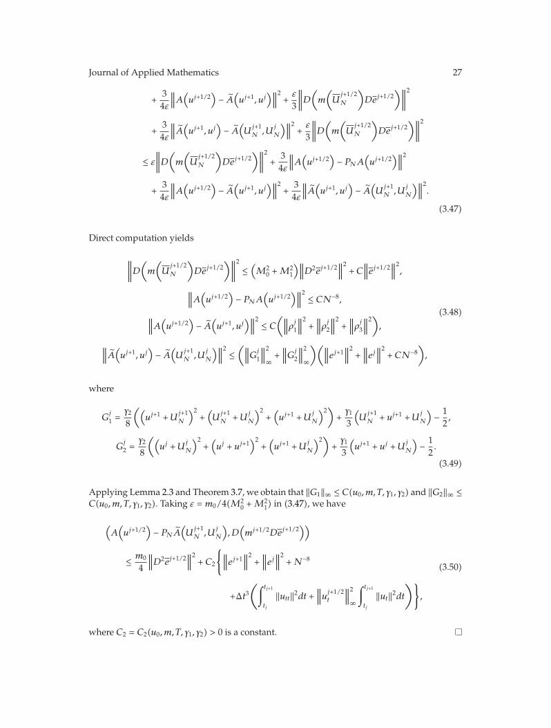
Journal of Applied Mathematics 27
+34ε
∥∥∥A(uj+1/2
)− A(uj+1, uj
)∥∥∥2+ε
3
∥∥∥∥D(m
(U
j+1/2N
)Dej+1/2
)∥∥∥∥
2
+34ε
∥∥∥A(uj+1, uj
)− A(U
j+1N ,U
j
N
)∥∥∥
2+ε
3
∥∥∥∥D(m
(U
j+1/2N
)Dej+1/2
)∥∥∥∥
2
≤ ε
∥∥∥∥D(m
(U
j+1/2N
)Dej+1/2
)∥∥∥∥
2
+34ε
∥∥∥A(uj+1/2
)− PNA
(uj+1/2
)∥∥∥
2
+34ε
∥∥∥A(uj+1/2
)− A(uj+1, uj
)∥∥∥
2+
34ε
∥∥∥A(uj+1, uj
)− A(U
j+1N ,U
j
N
)∥∥∥
2.
(3.47)
Direct computation yields
∥∥∥∥D(m
(U
j+1/2N
)Dej+1/2
)∥∥∥∥
2
≤(M2
0 +M21
)∥∥∥D2ej+1/2∥∥∥
2+ C∥∥∥ej+1/2
∥∥∥2,
∥∥∥A(uj+1/2
)− PNA
(uj+1/2
)∥∥∥2 ≤ CN−8,
∥∥∥A(uj+1/2
)− A(uj+1, uj
)∥∥∥2 ≤ C
(∥∥∥ρj
1
∥∥∥2+∥∥∥ρ
j
2
∥∥∥2+∥∥∥ρ
j
3
∥∥∥2),
∥∥∥A(uj+1, uj
)− A(U
j+1N ,U
j
N
)∥∥∥2 ≤(∥∥∥G
j
1
∥∥∥2
∞+∥∥∥G
j
2
∥∥∥2
∞
)(∥∥∥ej+1∥∥∥
2+∥∥∥ej∥∥∥
2+ CN−8
),
(3.48)
where
Gj
1 =γ2
8
((uj+1 +U
j+1N
)2+(U
j+1N +U
j
N
)2+(uj+1 +U
j
N
)2)+γ1
3
(U
j+1N + uj+1 +U
j
N
)− 1
2,
Gj
2 =γ2
8
((uj +U
j
N
)2+(uj + uj+1
)2+(uj+1 +U
j
N
)2)+γ1
3
(uj+1 + uj +U
j
N
)− 1
2.
(3.49)
Applying Lemma 2.3 and Theorem 3.7, we obtain that ‖G1‖∞ ≤ C(u0, m, T, γ1, γ2) and ‖G2‖∞ ≤C(u0, m, T, γ1, γ2). Taking ε = m0/4(M2
0 +M21) in (3.47), we have
(A(uj+1/2
)− PNA
(U
j+1N ,U
j
N
), D(mj+1/2Dej+1/2
))
≤ m0
4
∥∥∥D2ej+1/2∥∥∥
2+ C2
{∥∥∥ej+1∥∥∥
2+∥∥∥ej∥∥∥
2+N−8
+Δt3(∫ tj+1
tj
‖utt‖2dt +∥∥∥u
j+1/2t
∥∥∥2
∞
∫ tj+1
tj
‖ut‖2dt
)}
,
(3.50)
where C2 = C2(u0, m, T, γ1, γ2) > 0 is a constant.

28 Journal of Applied Mathematics
Lemma 3.6. Assume that u is the solution of (1.2)–(1.4). Then there exists a positive constant C =C(u0, m, γ1, γ2) > 0 such that
(D2uj+1/2 −A
(uj+1/2
), D
(m
(U
j+1/2N
)−m(uj+1/2
))Dej+1/2
)
≤ m0
4
∥∥∥D2ej+1/2
∥∥∥
2+ C
(∥∥∥ej+1/2
∥∥∥
2+N−8 + h3
∫ tj+1
tj
‖utt‖dt)
.
(3.51)
Proof. By (2.9), we have
∥∥∥D3uj+1/2 −DA
(uj+1/2
)∥∥∥∞≤∥∥∥D3uj+1/2
∥∥∥∞+∥∥∥A′(uj+1/2
)Duj+1/2
∥∥∥∞
≤∥∥∥D3uj+1/2
∥∥∥∞+∥∥∥A′(uj+1/2
)∥∥∥∞
∥∥∥Duj+1/2
∥∥∥∞≤ C.
(3.52)
In the other hand,
∥∥∥∥m(U
j+1/2N
)−m(uj+1/2
)∥∥∥∥
2
≤ M21
∥∥∥∥
(U
j+1/2N − uj+1/2
)∥∥∥∥
2
≤ C
∥∥∥∥∥U
j+1/2N − uj + uj+1
2
∥∥∥∥∥
2
+
∥∥∥∥∥uj + uj+1
2− uj+1/2
∥∥∥∥∥
2
≤ C∥∥∥ej+1/2
∥∥∥2+∥∥∥ηj+1/2
∥∥∥2+h3
96
∫ tj+1
tj
‖utt‖dt.
(3.53)
By Young inequality, we obtain
(D2uj+1/2 −A
(uj+1/2
), D
(m
(U
j+1/2N
)−m(uj+1/2
))Dej+1/2
)
= −(D3uj+1/2 −DA
(uj+1/2
), m
(U
j+1/2N
)−m(uj+1/2
)Dej+1/2
)
≤∥∥∥D3uj+1/2 −DA
(uj+1/2
)∥∥∥∞
∥∥∥∥m(U
j+1/2N
)−m(uj+1/2
)∥∥∥∥∥∥∥Dej+1/2
∥∥∥
≤ ε∥∥∥Dej+1/2
∥∥∥2+ Cε
∥∥∥∥m(U
j+1/2N
)−m(uj+1/2
)∥∥∥∥
2
≤ ε∥∥∥D2ej+1/2
∥∥∥∥∥∥ej+1/2
∥∥∥ + Cε
∥∥∥∥m(U
j+1/2N
)−m(uj+1/2
)∥∥∥∥
2
≤ ε∥∥∥D2ej+1/2
∥∥∥2+ Cε
(∥∥∥ej+1/2∥∥∥
2+N−8 + h3
∫ tj+1
tj
‖utt‖dt)
.
(3.54)
Choosing ε = m0/4 in the previous inequality leads to (3.51).
Finally, we obtain the main theorem of this paper.

Journal of Applied Mathematics 29
Theorem 3.7. Assume that u(x, t) is the solution of (1.2)–(1.4) and satisfies that
D4u ∈ L∞(QT ), ut ∈ L∞(QT ),
D2utt ∈ L2(QT ), uttt ∈ L2(QT ).(3.55)
Uj
N ∈ SN (j = 1, 2, . . . ,Λ) is the solution of the full-discretization (3.1) and (3.2). If h is sufficientlysmall, there exists a positive constant C such that, for any j = 0, 1, 2, . . . ,Λ,
∥∥∥ej+1
∥∥∥ =∥∥∥PNu
(tj+1) −U
j+1N
∥∥∥ ≤ C
(N−2 +
∥∥∥e0∥∥∥ + Bh2
), (3.56)
where B =∫ tj+1
0 (‖D2utt‖2 + ‖utt‖2 + ‖uttt‖2 + max0≤l≤j {‖ul+1/2t ‖2
∞} · ‖ut‖2)dt.
Proof. By (3.27), (3.36), (3.44), and (3.51), we have
∥∥∥ej+1∥∥∥
2 ≤∥∥∥ej∥∥∥
2+
h4
320
∫ tj+1
tj
‖uttt‖2dt + h∥∥∥ej+1/2
∥∥∥2
+ 2h
⎧⎨
⎩−⎛
⎝D2uj+1/2 − D2Uj+1N +D2U
j
N
2, D
(m
(U
j+1/2N
)Dej+1/2
)⎞
⎠
+(A(uj+1/2
)− A(U
j+1N ,U
j
N
), D
(m
(U
j+1/2N
)Dej+1/2
))
+(D2uj+1/2 −A
(uj+1/2
), D
(m
(U
j+1/2N
)−m(uj+1/2
))Dej+1/2
)⎫⎬
⎭
≤∥∥∥ej∥∥∥
2+ hC1
(N−4 +
∥∥∥ej+1∥∥∥
2+∥∥∥ej∥∥∥
2)
+ C2h4∫ tj+1
tj
(∥∥∥D2utt
∥∥∥2+ ‖utt‖2 + ‖uttt‖2 +
∥∥∥uj+1/2t
∥∥∥2
∞‖ut‖2
)dt,
(3.57)
where C1 = C1(m,u0, T, γ1, γ2) > 0 and C2 = C2(m,u0, T, γ1, γ2) > 0 are constants. Forsufficiently small h such that C1h ≤ 1/2, denoting C = 2(C1 + C2), we obtain
∥∥∥ej+1∥∥∥
2 ≤(
1 + Ch)∥∥∥ej
∥∥∥2+ C(hN−4 + h4Bj
), (3.58)
where
Bj =∫ tj+1
tj
(∥∥∥D2utt
∥∥∥2+ ‖utt‖2 + ‖uttt‖2 +
∥∥∥uj+1/2t
∥∥∥2
∞‖ut‖2
)dt. (3.59)

30 Journal of Applied Mathematics
By the Gronwall inequality of the discrete form, we obtain
∥∥∥ej+1
∥∥∥
2 ≤(
1 + Ch)j+1∥∥∥e0∥∥∥
2+ C
j∑
l=0
(1 + Ch
)l(htN−4 + h4Bl
)
≤ exp{C(j + 1)h}{∥∥∥e0∥∥∥
2+ C
j∑
l=0
(hN−4 + h4Bl
)}
≤ exp{C(j + 1)h}{∥∥∥e0∥∥∥
2+ C
(
jhN−4 + h4j∑
l=0
Bl
)}
.
(3.60)
Direct computation gives
j∑
l=0
Bl ≤∫ tj+1
0
(∥∥∥D2utt
∥∥∥2+ ‖utt‖2 + ‖uttt‖2 + max
0≤l≤j
{∥∥∥ul+1/2t
∥∥∥2
∞
}· ‖ut‖2
)dt. (3.61)
Then we complete the conclusion (3.56).
Furthermore, we get the following theorem.
Theorem 3.8. Assume u is the solution of (1.2)–(1.4) and satisfies that
D4u ∈ L∞(QT ), ut ∈ L∞(QT ),
D2utt ∈ L2(QT ), uttt ∈ L2(QT ).(3.62)
Uj
N ∈ SN (j = 1, 2, . . . ,Λ) is the solution of the full-discretization scheme (3.1)-(3.2), and U0
satisfies ‖e0‖ = ‖PNu0 − U0‖ ≤ CN−4. If h is sufficiently small, there exists a constant C =C(u0, m, T, γ1, γ2) > 0 such that
∥∥∥u(x, tj) −U
j
N
∥∥∥ ≤ C(N−2 + h2
), j = 1, 2, . . . ,Λ. (3.63)
4. Numerical Experiments
In this section, we apply the spectral method described in (3.1) and (3.2) to carry outnumerical computations to illustrate theoretical estimations in the previous section. Consider(2.2) with settings:
m(s) = m0 + s2, A(s) = s3 − s, (4.1)

Journal of Applied Mathematics 31
0
1
2
3
4
5
6×10⁻⁴
00.5
1
00.05
0.1
(a)
−2
0
2
4
6
8
10×10−4
00.5
10
0.050.1
(b)
Figure 1: The development of the solution of the full-discrete scheme when initial value is u0(x) =x5(1 − x)5 (a) and u0(x) = x5(1 − x)5ex (b).
where m0 > 0 is a constant. The full-discretization spectral method of (2.2) and (2.3) reads:find U
j
N =∑N
l=0 αjl cos lπx (j = 1, 2, . . . ,Λ) such that
⎛
⎝Uj+1N −U
j
N
h, v
⎞
⎠ +
⎛
⎝D2Uj+1N +D2U
j
N
2− PNA
(U
j+1N ,U
j
N
),
D
⎛
⎝m
⎛
⎝D2Uj+1N +D2U
j
N
2
⎞
⎠Dv
⎞
⎠
⎞
⎠ = 0,
(U0
N, v)− (u0, v) = 0.
(4.2)
In our computations we fix N = 32 and choose five different time-step sizes hk (k =1, 2, . . . , 5). Let Λk be the integer with hkΛk = T . Since we have no exact solution of (2.2) and(2.3), we take N = 32 and h0 = 0.15625×10⁻⁴ to compute an approximating solution UΛ0
N withh0Λ0 = T and regard this as an exact solution. we also choose five different time-step sizeshk (k = 1, 2, . . . , 5) with hkΛk = T to obtain five approximating solutions UΛk
N (k = 1, 2, . . . , 5)and compute the error estimation. Define an error function:
err(T, hk) =
(∫1
0
(UΛk
N −UΛ0N
)2dx
)1/2
. (4.3)
This function characterizes the estimations with respect to time-step size.
4.1. Example 1
Take m0 = 1 and T = 0.1. We also take two different initial functions u10(x) = x5(1 − x)5 and
u20 = x5(1 − x)5ex to carry out numerical computations. Figure 1 shows the development of
the solutions for time t from t = 0 to t = 0.1 with fixed step-size h0 = 0.15625 × 10⁻⁴.

32 Journal of Applied Mathematics
00.20.40.60.810
0.050.1−1
0
1
2
3
4
5
6×10⁻⁴
(a)
−2
0
2
4
6
8
10×10−4
00.5
10
0.050.1
(b)
Figure 2: The development of the solution of the full-discrete scheme with initial value u0(x) = x5(1 − x)5
(a) and u0(x) = x5(1 − x)5ex (b).
00.20.40.60.81 00.05
0.1−4
−2
0
2
4
6
8×10⁻³
(a)
0.015
0.01
0.005
0
−0.005
−0.01
−0.015
00.20.40.60.81 00.05
0.1
(b)
Figure 3: The development of the solution of the full-discrete scheme with initial value u0(x) = x5(1 − x)5
(a) and u0(x) = x5(1 − x)5ex (b).
Table 1: The error and the convergence order.
hk err1(0.1, hk) Order1 err2(0.1, hk) Order2
0.1 × 10⁻² 0.2441 × 10⁻⁶ — 0.2114 × 10⁻⁶ —0.5 × 10⁻³ 0.6332 × 10⁻⁷ 1.9466 0.5414 × 10⁻⁷ 1.96510.25 × 10−3 0.1186 × 10⁻⁷ 2.4159 0.1115 × 10⁻⁷ 2.27990.125 × 10−3 0.1938 × 10⁻⁸ 2.6142 0.1901 × 10⁻⁸ 2.55150.625 × 10−4 0.2504 × 10⁻⁹ 2.9518 0.2483 × 10⁻⁹ 2.9368
Table 2: The error and the convergence order.
hk err1(0.1, hk) Order1 err2(0.1, hk) Order2
0.1 × 10⁻² 0.4748 × 10⁻⁸ — 0.8864 × 10⁻⁸ —0.5 × 10⁻³ 0.8348 × 10⁻⁹ 2.5077 0.1577 × 10⁻⁸ 2.49070.25 × 10−3 0.1370 × 10⁻⁹ 2.6069 0.2440 × 10⁻⁹ 2.69220.125 × 10−3 0.2694 × 10⁻¹⁰ 2.3467 0.4457 × 10⁻¹⁰ 2.45250.625 × 10−4 0.6398 × 10⁻¹¹ 2.0741 0.1059 × 10⁻¹⁰ 2.0736

Journal of Applied Mathematics 33
Table 3: The error and the convergence order.
hk err1(0.1, hk) Order1 err2(0.1, hk) Order2
0.1 × 10⁻² 0.1150 × 10⁻⁵ — 0.5224 × 10⁻⁵ —0.5 × 10⁻³ 0.2872 × 10⁻⁶ 2.0013 0.1304 × 10⁻⁵ 2.00190.25 × 10−3 0.7158 × 10⁻⁷ 2.0043 0.3250 × 10⁻⁶ 2.00440.125 × 10−3 0.1769 × 10⁻⁷ 2.0170 0.8031 × 10⁻⁷ 2.01710.625 × 10−4 0.4211 × 10⁻⁸ 2.0704 0.1912 × 10⁻⁷ 2.0704
We also choose five different time-step sizes hk to carry out numerical computationsand apply the error function in (4.3) to illustrate the estimation and convergence order intime variable t, see Table 1.
4.2. Example 2
Take m0 = 0.05 and T = 0.1. We also take two different initial functions u10(x) = x5(1− x)5 and
u20 = x5(1 − x)5ex to carry out numerical computations. Figure 2 shows the development of
the solutions for time t from t = 0 to t = 0.1 with fixed step-sizes h0 = 0.15625 × 10⁻⁴.We also choose five different time-step sizes hk to carry out numerical computations
and apply the error function in (4.3) to illustrate the estimation and convergence order intime variable t, see Table 2.
4.3. Example 3
Take m0 = 0.005 and T = 0.1. We also take two different initial functions u10(x) = x5(1 − x)5
and u20 = x5(1 − x)5ex to carry out numerical computations. Figure 3 shows the development
of the solutions for time t from t = 0 to t = 0.1 with fixed step-sizes h0 = 0.15625 × 10⁻⁴.We also choose five different time-step sizes hk to carry out numerical computations
and apply the error function in (4.3) to illustrate the estimation and convergence order intime variable t, see Table 3.
Acknowledgment
This work is supported by NSFC no. 11071102.
References
[1] D. S. Cohen and J. D. Murray, “A generalized diffusion model for growth and dispersal in apopulation,” Journal of Mathematical Biology, vol. 12, no. 2, pp. 237–249, 1981.
[2] M. Hazewinkel, J. F. Kaashoek, and B. Leynse, “Pattern formation for a one-dimensional evolutionequation based on Thom’s river basin model,” in Disequilibrium and Self-Organisation (Klosterneuburg,1983/Windsor, 1985), vol. 30 of Mathematics and Its Applications, pp. 23–46, Reidel, Dordrecht, TheNetherlands, 1986.
[3] A. B. Tayler, Mathematical Models in Applied Mechanics, Oxford Applied Mathematics and ComputingScience Series, The Clarendon Press Oxford University Press, New York, NY, USA, 1986.
[4] C. M. Elliott and S. Zheng, “On the Cahn-Hilliard equation,” Archive for Rational Mechanics andAnalysis, vol. 96, no. 4, pp. 339–357, 1986.

34 Journal of Applied Mathematics
[5] X. Chen, “Global asymptotic limit of solutions of the Cahn-Hilliard equation,” Journal of DifferentialGeometry, vol. 44, no. 2, pp. 262–311, 1996.
[6] A. Novick-Cohen, “On Cahn-Hilliard type equations,” Nonlinear Analysis A, vol. 15, no. 9, pp. 797–814, 1990.
[7] S. Zheng, “Asymptotic behavior of solution to the Cahn-Hillard equation,” Applicable Analysis, vol.23, no. 3, pp. 165–184, 1986.
[8] A. Voigt and K.-H. Hoffman, “Asymptotic behavior of solutions to the Cahn-Hilliard equation inspherically symmetric domains,” Applicable Analysis, vol. 81, no. 4, pp. 893–903, 2002.
[9] X. Chen and M. Kowalczyk, “Existence of equilibria for the Cahn-Hilliard equation via localminimizers of the perimeter,” Communications in Partial Differential Equations, vol. 21, no. 7-8, pp. 1207–1233, 1996.
[10] B. E. E. Stoth, “Convergence of the Cahn-Hilliard equation to the Mullins-Sekerka problem inspherical symmetry,” Journal of Differential Equations, vol. 125, no. 1, pp. 154–183, 1996.
[11] J. Bricmont, A. Kupiainen, and J. Taskinen, “Stability of Cahn-Hilliard fronts,” Communications on Pureand Applied Mathematics, vol. 52, no. 7, pp. 839–871, 1999.
[12] E. A. Carlen, M. C. Carvalho, and E. Orlandi, “A simple proof of stability of fronts for theCahn-Hilliard equation,” Communications in Mathematical Physics, vol. 224, no. 1, pp. 323–340, 2001,Dedicated to Joel L. Lebowitz.
[13] A. Miranville and S. Zelik, “Exponential attractors for the Cahn-Hilliard equation with dynamicboundary conditions,” Mathematical Methods in the Applied Sciences, vol. 28, no. 6, pp. 709–735, 2005.
[14] J. Pruss, R. Racke, and S. Zheng, “Maximal regularity and asymptotic behavior of solutions for theCahn-Hilliard equation with dynamic boundary conditions,” Annali di Matematica Pura ed ApplicataIV, vol. 185, no. 4, pp. 627–648, 2006.
[15] R. Racke and S. Zheng, “The Cahn-Hilliard equation with dynamic boundary conditions,” Advancesin Differential Equations, vol. 8, no. 1, pp. 83–110, 2003.
[16] H. Wu and S. Zheng, “Convergence to equilibrium for the Cahn-Hilliard equation with dynamicboundary conditions,” Journal of Differential Equations, vol. 204, no. 2, pp. 511–531, 2004.
[17] J. W. Barrett and J. F. Blowey, “An error bound for the finite element approximation of a model forphase separation of a multi-component alloy,” IMA Journal of Numerical Analysis, vol. 16, no. 2, pp.257–287, 1996.
[18] J. W. Barrett and J. F. Blowey, “Finite element approximation of a model for phase separation of amulti-component alloy with non-smooth free energy,” Numerische Mathematik, vol. 77, no. 1, pp. 1–34,1997.
[19] J. W. Barrett and J. F. Blowey, “Finite element approximation of a degenerate Allen-Cahn/Cahn-Hilliard system,” SIAM Journal on Numerical Analysis, vol. 39, no. 5, pp. 1598–1624, 2001/02.
[20] J. W. Barrett, J. F. Blowey, and H. Garcke, “Finite element approximation of the Cahn-Hilliard equationwith degenerate mobility,” SIAM Journal on Numerical Analysis, vol. 37, no. 1, pp. 286–318, 1999.
[21] P. K. Chan and A. D. Rey, “A numerical method for the nonlinear Cahn-Hilliard equation withnonperiodic boundary conditions,” Computational Materials Science, vol. 3, no. 3, pp. 377–392, 1995.
[22] C. M. Elliott, D. A. French, and F. A. Milner, “A second order splitting method for the Cahn-Hilliardequation,” Numerische Mathematik, vol. 54, no. 5, pp. 575–590, 1989.
[23] C. M. Elliott and D. A. French, “A nonconforming finite-element method for the two-dimensionalCahn-Hilliard equation,” SIAM Journal on Numerical Analysis, vol. 26, no. 4, pp. 884–903, 1989.
[24] C. M. Elliott and S. Larsson, “Error estimates with smooth and nonsmooth data for a finite elementmethod for the Cahn-Hilliard equation,” Mathematics of Computation, vol. 58, no. 198, p. 603–630, S33–S36, 1992.
[25] E. V. L. de Mello and O. T. da Silveira Filho, “Numerical study of the Cahn-Hilliard equation in one,two and three dimensions,” Physica A, vol. 347, no. 1–4, pp. 429–443, 2005.
[26] D. Furihata, “A stable and conservative finite difference scheme for the Cahn-Hilliard equation,”Numerische Mathematik, vol. 87, no. 4, pp. 675–699, 2001.
[27] J. Kim, “A numerical method for the Cahn-Hilliard equation with a variable mobility,” Communica-tions in Nonlinear Science and Numerical Simulation, vol. 12, no. 8, pp. 1560–1571, 2007.
[28] J. Kim, K. Kang, and J. Lowengrub, “Conservative multigrid methods for Cahn-Hilliard fluids,”Journal of Computational Physics, vol. 193, no. 2, pp. 511–543, 2004.
[29] Z. Z. Sun, “A second-order accurate linearized difference scheme for the two-dimensional Cahn-Hilliard equation,” Mathematics of Computation, vol. 64, no. 212, pp. 1463–1471, 1995.
[30] F. L. Bai, L. Yin, and Y. K. Zou, “A pseudo-spectral method for the Cahn-Hilliard equation,” Journal ofJilin University, vol. 41, no. 3, pp. 262–268, 2003.

Journal of Applied Mathematics 35
[31] Y. He and Y. Liu, “Stability and convergence of the spectral Galerkin method for the Cahn-Hilliardequation,” Numerical Methods for Partial Differential Equations, vol. 24, no. 6, pp. 1485–1500, 2008.
[32] P. Howard, “Spectral analysis of planar transition fronts for the Cahn-Hilliard equation,” Journal ofDifferential Equations, vol. 245, no. 3, pp. 594–615, 2008.
[33] X. Ye, “The Fourier collocation method for the Cahn-Hilliard equation,” Computers &Mathematics withApplications, vol. 44, no. 1-2, pp. 213–229, 2002.
[34] X. Ye, “The Legendre collocation method for the Cahn-Hilliard equation,” Journal of Computational andApplied Mathematics, vol. 150, no. 1, pp. 87–108, 2003.
[35] X. Ye and X. Cheng, “The Fourier spectral method for the Cahn-Hilliard equation,” AppliedMathematics and Computation, vol. 171, no. 1, pp. 345–357, 2005.
[36] B. Nicolaenko, B. Scheurer, and R. Temam, “Some global dynamical properties of a class of patternformation equations,” Communications in Partial Differential Equations, vol. 14, no. 2, pp. 245–297, 1989.
[37] Q. Du and R. A. Nicolaides, “Numerical analysis of a continuum model of phase transition,” SIAMJournal on Numerical Analysis, vol. 28, no. 5, pp. 1310–1322, 1991.
[38] D. Furihata, “Finite difference schemes for ∂u/∂t = (∂/∂x)αδG/δu that inherit energy conservationor dissipation property,” Journal of Computational Physics, vol. 156, no. 1, pp. 181–205, 1999.
[39] C. Canuto and A. Quarteroni, “Error estimates for spectral and pseudospectral approximations ofhyperbolic equations,” SIAM Journal on Numerical Analysis, vol. 19, no. 3, pp. 629–642, 1982.
[40] J. X. Yin, “On the existence of nonnegative continuous solutions of the Cahn-Hilliard equation,”Journal of Differential Equations, vol. 97, no. 2, pp. 310–327, 1992.
[41] J. X. Yin, “On the Cahn-Hilliard equation with nonlinear principal part,” Journal of Partial DifferentialEquations, vol. 7, no. 1, pp. 77–96, 1994.
[42] C. C. Liu, Y. W. Qi, and J. X. Yin, “Regularity of solutions of the Cahn-Hilliard equation with non-constant mobility,” Acta Mathematica Sinica, vol. 22, no. 4, pp. 1139–1150, 2006.
[43] J. Yin and C. Liu, “Regularity of solutions of the Cahn-Hilliard equation with concentrationdependent mobility,” Nonlinear Analysis A, vol. 45, no. 5, pp. 543–554, 2001.
[44] D. Kay and R. Welford, “A multigrid finite element solver for the Cahn-Hilliard equation,” Journal ofComputational Physics, vol. 212, no. 1, pp. 288–304, 2006.

Hindawi Publishing CorporationJournal of Applied MathematicsVolume 2012, Article ID 150145, 20 pagesdoi:10.1155/2012/150145
Research ArticleViscosity Approximation Methods forEquilibrium Problems, Variational InequalityProblems of Infinitely Strict Pseudocontractions inHilbert Spaces
Aihong Wang
College of Science, Civil Aviation University of China, Tianjin 300300, China
Correspondence should be addressed to Aihong Wang, [email protected]
Received 23 April 2012; Accepted 2 August 2012
Academic Editor: Hong-Kun Xu
Copyright q 2012 Aihong Wang. This is an open access article distributed under the CreativeCommons Attribution License, which permits unrestricted use, distribution, and reproduction inany medium, provided the original work is properly cited.
We introduce an iterative scheme by the viscosity approximation method for finding a commonelement of the set of the solutions of the equilibrium problem and the set of fixed points of infinitelystrict pseudocontractive mappings. Strong convergence theorems are established in Hilbert spaces.Our results improve and extend the corresponding results announced by many others recently.
1. Introduction
Let H be a real Hilbert space and let C be a nonempty convex subset of H.A mapping S of C is said to be a κ-strict pseudocontraction if there exists a constant
κ ∈ [0, 1) such that
∥∥Sx − Sy∥∥2 ≤ ∥∥x − y
∥∥2 + κ∥∥(I − S)x − (I − S)y
∥∥2, (1.1)
for all x, y ∈ C; see [1]. We denote the set of fixed points S by F(S) (i.e., F(S) = {x ∈ C : Sx =x}).
Note that the class of strict pseudocontraction strictly includes the class of nonexpan-sive mappings which are mappings S on C such that
∥∥Sx − Sy∥∥ ≤ ∥∥x − y
∥∥, (1.2)

2 Journal of Applied Mathematics
for all x, y ∈ C. That is, S is nonexpansive if and only if S is a 0-strict pseudocontraction.Let Φ be a bifunction from C × C to R, where R is the set of real numbers. The equilibriumproblem for Φ : C × C → R is to find x ∈ C such that
Φ(x, y
) ≥ 0, ∀y ∈ C. (1.3)
The set of solutions of (1.3) is denoted by EP(Φ). Given a mapping B : C → H, let Φ(x, y) =〈Bx, y − x〉 for all x, y ∈ C. Then the classical variational inequality problem is to find x ∈ Csuch that 〈Bx, y − x〉 ≥ 0. We denote the solution of the variational inequality by VI(C,B);that is
VI(C,B) ={x ∈ C :
⟨Bx, y − x
⟩ ≥ 0}. (1.4)
Let A be a strongly positive linear-bounded operator on H if there is a constant γ > 0 withproperty
〈Ax, x〉 ≥ γ‖x‖2, ∀x ∈ H. (1.5)
A typical problem is to minimize a quadratic function over the set of the fixed points anonexpansive mapping on a real Hilbert space H:
minx∈E
12〈Ax, x〉 − 〈x, b〉, (1.6)
where A is a linear-bounded operator, E is the fixed point set of a nonexpansive mappingS on H, and b is a given point in H. The problem (1.3) is very general in the sense that itincludes, as special cases, optimization problems, variational inequalities, minimax problems,the Nash equilibrium problem in noncooperative games, and others; see [1–11]. In particular,Combettes and Hirstoaga [4] proposed several methods for solving the equilibrium problem.On the other hand, Mann [6], Shimoji and Takahashi [8] considered iterative schemes forfinding a fixed point of a nonexpansive mapping. Further, Acedo and Xu [12] projected newiterative methods for finding a fixed point of strict pseudocontractions.
In 2006, Marino and Xu [7] introduced the general iterative method: for x1 = x ∈ C,
xn+1 = αnγf(xn) + (I − αnA)Txn, n ≥ 1. (1.7)
They proved that the sequence {xn} of parameters satisfies appropriate condition and that thesequence {xn} generated by (1.7) converges strongly to the unique solution of the variationalinequality 〈(γf − A)q, p − q〉 ≤ 0, p ∈ F(T). Recently, Liu [5] considered a general iterativemethod for equilibrium problems and strict pseudocontractions:
Φ(un, y
)+
1rn
⟨y − un, un − xn
⟩ ≥ 0, ∀y ∈ C,
yn = βnun +(1 − βn
)Sun,
xn+1 = εnγf(xn) + (I − εnA)un, ∀n ≥ 1,
(1.8)

Journal of Applied Mathematics 3
where S is a k-strict pseudocondition mapping and {εn}, {βn} are sequences in (0, 1). Theyproved that under certain appropriate conditions over {εn}, {βn}, and {rn}, the sequences{xn} and {un} both converge strongly to some q ∈ F(S)
⋂EP(Φ), which solves some
variational inequality problems. Tian [10] proposed a new general iterative algorithm: fornonexpansive mapping T : H → H with F(T)/=φ,
xn+1 = αnγf(xn) +(I − μαnF
)Txn, ∀n ≥ 1, (1.9)
where F is a k-Lipschitzian and η-strong monotone operator. He obtained that the sequencexn generated by (1.9) converges to a point q in F(T), which is the unique solution of thevariational inequality 〈(γf −A)q, p − q〉 ≤ 0, p ∈ F(T). Very recently, Wang [13] considered ageneral composite iterative method for infinite family strict pseudocontractions: for x1 = x ∈C,
yn = βnxn +(1 − βn
)Wnxn,
xn+1 = αnγf(xn) +(I − μαnF
)yn, ∀n ≥ 1,
(1.10)
where Wn is a mapping defined by (2.5), F is a k-Lipschitzian, and η-strongly monotoneoperator. With some appropriate condition, the sequence {xn} generated by (1.10) convergesstrongly to a common element of the fixed point of an infinite family of λi-strictlypseudocontractive mapping, which is a unique solution of the variational inequality 〈(γf −A)q, p − q〉 ≤ 0, p ∈ F(T). Kumam proposed many algorithms for the equilibrium andthe fixed point problems with k-strict pseudoconditions; see [14–16]. In particular, in 2011,Kumam and Jaiboon [14] considered a system of mixed equilibrium problems, variationalinequality problems, and strict pseudocontractive mappings:
x1 ∈ E, un ∈ E, vn ∈ E,
un = Tφ1,ϕr xn,
vn = Tφ2,ϕs xn,
zn = PE
(un − μnCun
),
yn = PE(vn − λnCvn),
kn = anSkxn + bnyn + cnzn,
xn+1 = εnγf(xn) + βnxn +((
1 − βn)I − εnA
)kn, ∀n ≥ 1,
(1.11)
where S is a k-strict pseudocondition mapping. They proved that under certain appropriateconditions over {εn}, {βn}, {rn}, {an}, {bn}, {cn}, {λn}, and {μn}, the sequence {xn} convergesstrongly to a point q ∈ Θ which is the unique solution of the variational inequality 〈(A −γf)q, x − q〉 ≥ 0. Inprasit [17] proposed a viscosity approximation methods to solving thegeneralized equilibrium and fixed point problems of finite family of nonexpansive mappingin Hilbert spaces.

4 Journal of Applied Mathematics
In this paper, motivated by the above facts, we use the viscosity approximation methodto find a common element of the set of solutions of the equilibrium problem VI(C,B) and theset of fixed points of a infinite family of strict pseudocontractions.
2. Preliminaries
Throughout this paper, we always write ⇀ for weak convergence and → for strongconvergence. We need some facts and tools in a real Hilbert space H which are listed asbelow.
Lemma 2.1. LetH be a real Hilbert space. There hold the following identities:
(i) ‖x − y‖2 = ‖x‖2 − ‖y‖2 − 2〈x − y, y〉, ∀x, y ∈ H,
(ii) ‖tx + (1 − t)y‖2 = t‖x‖2 + (1 − t)‖y‖2 − t(1 − t)‖x − y‖2, ∀t ∈ [0, 1], ∀x, y ∈ H.
Lemma 2.2 (see [18]). Assume that {αn} is a sequence of nonnegative real numbers such that
αn+1 ≤ (1 − ρn)αn + σn, (2.1)
where {ρn} is a sequence in (0, 1) and {σn} is a sequence such that
(i)∑∞
n=1 ρn = ∞,
(ii) lim supn→∞(σn/ρn) ≤ 0 or∑∞
n=1 |σn| < ∞.
Then limn→∞an = 0.
Recall that given a nonempty closed convex subset C of a real Hilbert space H, for anyx ∈ H, there exists a unique nearest point in C, denoted by PCx, such that
‖x − PCx‖ ≤ ∥∥x − y∥∥, (2.2)
for all y ∈ C. Such a PC is called the metric (or the nearest point) projection of H onto C. Aswe all know, y = PCx if and only if there holds the relation:
⟨x − y, y − z
⟩ ≥ 0 ∀z ∈ C. (2.3)
Lemma 2.3 (see [13]). Let A : H → H be an L-Lipschitzian and η-strongly monotone operator ona Hilbert spaceH with L > 0, η > 0, 0 < μ < 2η/L2, and 0 < t < 1. Then S = (I − tμA) : H → His a contraction with contractive coefficient 1 − tτ and τ = (1/2)μ(2η − μL2).
Lemma 2.4 (see [1]). Let S : C → C be a κ-strict pseudocontraction. Define T : C → C byTx = λx + (1 − λ)Sx for each x ∈ C. Then, as λ ∈ [κ, 1), T is a nonexpansive mapping such thatF(T) = F(S).

Journal of Applied Mathematics 5
Lemma 2.5 (see [10]). Let H be a Hilbert space and f : H → H a contraction with coefficient0 < α < 1, and A : H → H an L-Lipschitzian continuous operator and η-strongly monotone withL > 0, η > 0. Then for 0 < γ < μη/α,
⟨x − y,
(μA − γf
)x − (μA − γf
)y⟩ ≥ (μη − γα
)∥∥x − y∥∥2
, x, y ∈ H. (2.4)
That is, μA − γf is strongly monotone with coefficient μη − γα.
Let {Sn} be a sequence of κn-strict pseudo-concontractions. Define S′n = θnI + (1 −
θn)Sn, θn ∈ [κn, 1). Then, by Lemma 2.4, S′n is nonexpansive. In this paper, we consider the
mapping Wn defined by
Un,n+1 = I,
Un,n = tnS′nUn,n+1 + (1 − tn)I,
Un,n−1 = tn−1S′n−1Un,n + (1 − tn−1)I,
· · · ,Un,i = tiS
′iUn,i+1 + (1 − ti)I,
· · · ,Un,2 = t2S
′2Un,3 + (1 − t2)I,
Wn = Un,1 = t1S′1Un,2 + (1 − t1)I.
(2.5)
Lemma 2.6 (see [8]). Let C be a nonempty closed convex subset of a strictly convex Banach space E,let S′
1, S′2, . . . be nonexpansive mappings of C into itself such that ∩∞
i=1F(S′i)/= ∅, and let t1, t2, . . . be
real numbers such that 0 < ti ≤ b < 1, for every i = 1, 2, . . .. Then, for any x ∈ C and k ∈ N, the limitlimn→∞Un,kx exists.
Using Lemma 2.6, one can define the mapping W of C into itself as follows:
Wx := limn→∞
Wnx = limn→∞
Un,1x, x ∈ C. (2.6)
Lemma 2.7 (see [8]). Let C be a nonempty closed convex subset of a strictly convex Banach space E.Let S′
1, S′2, . . . be nonexpansive mappings of C into itself such that ∩∞
i=1F(S′i)/= ∅, and let t1, t2, . . . be
real numbers such that 0 < ti ≤ b < 1, for all i ≥ 1. If K is any bounded subset of C, then
limn→∞
supx∈K
‖Wx −Wnx‖ = 0. (2.7)
Lemma 2.8 (see [3]). Let C be a nonempty closed convex subset of a Hilbert spaceH, let {S′i : C →
C} be a family of infinite nonexpansive mappings with ∩∞i=1F(S
′i)/= ∅, and let t1, t2, . . . be real numbers
such that 0 < ti ≤ b < 1, for every i = 1, 2, . . .. Then F(W) = ∩∞i=1F(S
′i).

6 Journal of Applied Mathematics
For solving the equilibrium problem, let us assume that the bifunction Φ satisfies thefollowing conditions:
(A1) Φ(x, x) = 0 for all x ∈ C;
(A2) Φ is monotone; that is Φ(x, y) + Φ(y, x) ≤ 0 for any x, y ∈ C;
(A3) for each x, y, z ∈ C, lim supt→ 0Φ(tz + (1 − t)x, y) ≤ Φ(x, y);
(A4) Φ(x, ·) is convex and lower semicontinuous for each x ∈ C.
We recall some lemmas which will be needed in the rest of this paper.
Lemma 2.9 (see [2]). Let C be a nonempty closed convex subset ofH, letΦ be bifunction from C×Cto R satisfying (A1)–(A4), and let r > 0 and x ∈ H. Then there exists z ∈ C such that
Φ(z, y
)+
1r
⟨y − z, z − x
⟩ ≥ 0, ∀y ∈ C. (2.8)
Lemma 2.10 (see [4]). Let φ be a bifunction from C × C into R satisfying (A1)–(A4). Then, for anyr > 0 and x ∈ H, there exists z ∈ C such that
Φ(z, y
)+
1r
⟨y − z, z − x
⟩ ≥ 0, ∀y ∈ C. (2.9)
Further, if Trx = {z ∈ C;Φ(z, y) + (1/r)〈y − z, z − x〉 ≥ 0, ∀y ∈ C}, then the following hold:
(1) Tr is single-valued;
(2) Tr is firmly nonexpansive;
(3) F(Tr) = EP(φ);
(4) EP(φ) is closed and convex.
Lemma 2.11 (see [9]). Let {xn} and {zn} be bounded sequences in a Banach space, and let {βn} bea sequence of real numbers such that 0 < lim infn→∞βn ≤ lim supn→∞βn < 1 for all n = 0, 1, 2, . . ..Suppose that xn+1 = (1−βn)zn + βnxn for all n = 0, 1, 2, . . .. and lim supn→∞‖zn+1 −zn‖−‖xn+1 −xn‖ ≤ 0. Then limn→∞‖zn − xn‖ = 0.
Lemma 2.12 (see [11]). Let C,H, F, and Trx be as in Lemma 2.9. Then the following holds:
‖Tsx − Ttx‖2 ≤ 〈Tsx − Ttx, Tsx − x〉, (2.10)
for all s, t > 0, and x ∈ H.
Lemma 2.13 (see [13]). Let H be a Hilbert space, and let C be a nonempty closed convex subsetof H, and T : C → C a nonexpansive mapping with F(T)/= ∅. If {xn} is a sequence in C weaklyconverging to x and if {(I − T)xn} converges strongly to y, then (I − T)x = y.
3. Main Results
Now we start and prove our main result of this paper.

Journal of Applied Mathematics 7
Theorem 3.1. Let C be a nonempty closed convex subset of a real Hilbert space H. Let φ bea bifunction from C × C → R satisfying (A1)–(A4). Let Si : C → C be a family κi-strictpseudocontractions for some 0 ≤ κi < 1. Assume the setΩ = VI(C,B)∩∞
i=1F(Si)∩EP(φ)/= ∅. Let f bea contraction of H into itself with α ∈ (0, 1), and let A be a strongly positive linear bounded operatoron H with coefficient γ > 0 and 0 < γ < γ/γ . Let B : C → H be an ξ-inverse strongly monotonemapping. Let Wn be the mapping generated by S′
i and ti as in (2.5). Let {xn} be a sequence generatedby the following algorithm:
φ(zn, y
)+
1λn
⟨y − zn, zn − xn
⟩ ≥ 0,
yn = PC
(I − μnB
)zn,
Kn = αnxn + (1 − αn)Wnyn,
xn+1 = εnγf(xn) + βnxn +((
1 − βn)I − εnA
)Kn,
(3.1)
where {εn}, {βn}, {αn}, and {λn} are sequences in (0, 1). Assume that the control sequences satisfythe following restrictions:
(i) limn→∞εn = 0 and Σ∞n=1εn = ∞;
(ii) 0 < lim infn→∞βn ≤ lim supn→∞βn < 1;
(iii) 0 < limn→∞(λn/λn+1) = 1;
(iv) limn→∞|αn+1 − αn| = 0;
(v) 0 < μn ≤ 2ξ;
(vi) limn→∞αn = a.
Then {xn} converges strongly to q ∈ Ω which is the unique solution of the variational inequality
⟨(A − γf
)q, x − q
⟩ ≥ 0, ∀x ∈ Ω, (3.2)
or equivalent q = PΩ(I −A + γf)(q), where P is a metric projection mapping form H onto Ω.
Proof. Since εn → 0, as n → ∞, we may assume, without loss of generality, that εn ≤ (1 −βn)‖A‖−1 for all n ∈ N. By Lemma 2.3, we know that if 0 ≤ ρ ≤ ‖A‖−1, then ‖I − ρA‖ ≤ 1 − ργ .We will assume that ‖I − A‖ ≤ 1 − γ . Since A is a strongly positive bounded linear operatoron H, we have
‖A‖ = sup{|〈Ax, x〉| : x ⊆ H, ‖x‖ = 1}. (3.3)
Observe that
⟨((1 − βn
)I − εnA
)x, x
⟩=(1 − βn
)‖x‖2 − εn〈Ax, x〉
≥ (1 − βn)‖x‖2 − εn‖A‖
≥ 0.
(3.4)

8 Journal of Applied Mathematics
So this shows that (1 − βn)I − εnA is positive. It follows that
∥∥(1 − βn
)I − εnA
∥∥ = sup
{∣∣⟨((1 − βn)I − εnA
)x, x
⟩∣∣ : x ⊆ H, ‖x‖ = 1}
= sup{
1 − βn − εn〈Ax, x〉x ⊆ H, ‖x‖ = 1} ≤ 1 − βn − εnγ.
(3.5)
Step 1. We claim that the mapping PΩ(I −A + γf) where Ω =⋂∞
i=1 F(Si)⋂EP(Φ) has a
unique fixed point. Let f be a contraction of H into itself with α ∈ (0, 1). Then, we have
∥∥PC
(I −A + γf
)(x) − PC
(I −A + γf
)(y)∥∥ ≤ ∥∥(I −A + γf
)(x) − (I −A + γf
)(y)∥∥
≤ ‖I −A‖∥∥x − y∥∥ + γ
∥∥f(x) − f
(y)∥∥
≤ (1 − γ)∥∥x − y
∥∥ + γα∥∥x − y
∥∥
=(1 − (γ − γα
))∥∥x − y∥∥,
(3.6)
for all x, y ∈ H. Since 0 < 1 − (γ − γα) < 1, it follows that PΩ(I − A + γf) is a contraction ofH into itself. Therefore the Banach contraction mapping principle implies that there exists aunique element q ∈ H such that q = PΩ(I −A + γf)(q).
Step 2. We shall show that (I − μnB) is nonexpansive. Let x, y ∈ C. Since B is ξ-inversestrongly monotone and λn < 2α for all n ∈ N, we obtain
∥∥(I − μnB)x − (I − μnB
)y∥∥2 =
∥∥x − y − μn
(Bx − By
)∥∥2
=∥∥x − y
∥∥2 − 2μn
⟨x − y, Bx − By
⟩
+ μ2n
∥∥Bx − By∥∥2
≤ ∥∥x − y∥∥2 − 2ξμn
∥∥Bx − By∥∥2 + μ2
n
∥∥Bx − By∥∥2
=∥∥x − y
∥∥2 + μn
(μn − 2ξ
)∥∥Bx − By∥∥2 ≤ ∥∥x − y
∥∥2,
(3.7)
where μn ≤ 2ξ, for all n ∈ N. So we have that the mapping (I − λnA) is nonexpansive.Step 3. We claim that {xn} is bounded.Let p ∈ Ω; from Lemma 2.10, we have
p = PC
(p − μnBp
)= Tλnp,
∥∥zn − p∥∥ =
∥∥Tλnxn − Tλnp∥∥
≤ ∥∥xn − p∥∥.
(3.8)

Journal of Applied Mathematics 9
Note that
∥∥yn − p
∥∥ =
∥∥PC
(I − μnB
)zn − p
∥∥
=∥∥PC
(I − μnB
)zn − PC
(I − μnB
)p∥∥
≤ ∥∥(zn − μnBzn) − (p − μnBp
)∥∥
=∥∥(I − μnB
)(zn − p
)∥∥
≤ ∥∥zn − p∥∥
≤ ∥∥xn − p∥∥,
∥∥Kn − p
∥∥ =
∥∥αnxn + (1 − αn)Wnyn − p
∥∥
=∥∥αn
(xn − p
)+ (1 − αn)
(Wnyn − p
)∥∥
≤ αn
∥∥xn − p∥∥ + (1 − αn)
∥∥Wnyn − p∥∥
≤ αn
∥∥xn − p∥∥ + (1 − αn)
∥∥yn − p∥∥
≤ ∥∥xn − p∥∥.
(3.9)
It follows that
∥∥xn+1 − p∥∥ =
∥∥εnγf(xn) + βnxn +((
1 − βn)I − εnA
)Kn − p
∥∥
=∥∥εn
(γf(xn) −Ap
)+ βn
(xn − p
)+((
1 − βn)I − εnA
)(Kn − p
)∥∥
≤ εn∥∥γf(xn) −Ap
∥∥ + βn∥∥xn − p
∥∥ +(1 − βn − εnγ
)∥∥Kn − p∥∥
≤ εn∥∥γf(xn) −Ap
∥∥ + βn∥∥xn − p
∥∥ +(1 − βn − εnγ
)∥∥xn − p∥∥
≤ (1 − εnγ)∥∥xn − p
∥∥ + εnγ∥∥f(xn) − f
(p)∥∥ + εn
∥∥γf(p) −Ap
∥∥
≤ (1 − εnγ)∥∥xn − p
∥∥ + εnγα∥∥xn − p
∥∥ + εn∥∥γf
(p) −Ap
∥∥
=(1 − (γ − αγ
)εn)∥∥xn − p
∥∥ +(γ − αγ
)εn
∥∥γf(p) −Ap
∥∥
γ − αγ
≤ max
{∥∥xn − p
∥∥,
∥∥γf(p) −Ap
∥∥
γ − αγ
}
.
(3.10)
By simple induction, we have
∥∥xn − p∥∥ ≤ max
{∥∥x1 − p
∥∥,
∥∥γf(p) −Ap
∥∥
γ − αγ
}
, ∀n ∈ N. (3.11)
Hence {xn} is bounded. This implies that {Kn}, {f(xn)} are also bounded.

10 Journal of Applied Mathematics
Step 4. Show that lim supn→∞‖xn+1 − xn‖ = 0.Observing that zn = Tλnxn and zn+1 = Tλn+1 , we get
‖zn+1 − zn‖ = ‖Tλn+1xn+1 − Tλnxn‖= ‖Tλn+1xn+1 − Tλn+1xn + Tλn+1xn − Tλnxn‖≤ ‖xn+1 − xn‖ + ‖Tλn+1xn − Tλnxn‖.
(3.12)
By Lemma 2.10, we obtain
Φ(Tλnxn, y
)+
1λn
⟨y − Tλnxn, Tλnun − xn
⟩ ≥ 0, ∀y ∈ C,
Φ(Tλn+1xn, y
)+
1λn+1
⟨y − Tλn+1xn, Tλn+1xn − xn
⟩ ≥ 0, ∀y ∈ C.
(3.13)
In particular, we have
Φ(Tλnxn, Tλn+1xn) +1λn
〈Tλn+1xn − Tλnxn, Tλnxn − xn〉 ≥ 0,
Φ(Tλn+1xn, Tλnxn) +1
λn+1〈Tλnxn − Tλn+1xn, Tλn+1xn − xn〉 ≥ 0.
(3.14)
Summing up (3.14) and using (A2), we obtain
1λn+1
〈Tλnxn − Tλn+1xn, Tλn+1xn − xn〉 + 1λn
〈Tλn+1xn − Tλnxn, Tλnxn − xn〉 ≥ 0, (3.15)
for all y ∈ C. It follows that
⟨Tλnxn − Tλn+1xn,
Tλn+1xn − xn
λn+1− Tλnxn − xn
λn
⟩≥ 0. (3.16)
This implies
0 ≤⟨Tλn+1xn − Tλnxn, Tλnxn − xn − λn
λn+1(Tλn+1xn − xn)
⟩
=⟨Tλn+1xn − Tλnxn, Tλnxn − Tλn+1xn +
(1 − λn
λn+1
)(Tλn+1xn − xn)
⟩.
(3.17)
It follows that
‖Tλn+1xn − Tλnxn‖2 ≤∣∣∣∣1 − λn
λn+1
∣∣∣∣‖Tλn+1xn − Tλnxn‖(‖Tλn+1xn‖ + ‖xn‖). (3.18)

Journal of Applied Mathematics 11
Hence, we obtain
‖Tλn+1xn − Tλnxn‖2 ≤∣∣∣∣1 − λn
λn+1
∣∣∣∣L, (3.19)
where L = sup{‖xn‖ + ‖Tλn+1xn‖ : n ∈ N}. By (3.12) and (3.19), we obtain
‖zn+1 − zn‖ ≤ ‖un+1 − un‖ + ‖Tλn+1un − Tλnun‖
≤ ‖xn+1 − xn‖ +∣∣∣∣1 − λn
λn+1
∣∣∣∣L,
∥∥yn+1 − yn
∥∥ =
∥∥PC
(I − μnB
)zn+1 − PC
(I − μnB
)zn∥∥
≤ ∥∥(I − μnB)(zn+1 − zn)
∥∥
≤ ‖zn+1 − zn‖ ≤ ‖xn+1 − xn‖ +∣∣∣∣1 − λn
λn+1
∣∣∣∣L.
(3.20)
From (2.5), we have
∥∥Wn+1yn −Wnyn
∥∥ =∥∥t1S′
1Un+1,2yn − t1S′1Un,2yn
∥∥
≤ t1∥∥Un+1,2yn −Un,2
∥∥
≤ t1∥∥t2S′
2Un+1,3yn − t2S′2Un,3yn
∥∥
≤ t1t2∥∥Un+1,3yn −Un,3yn
∥∥
≤ · · ·
≤ M1
n∏
i=1
ti,
(3.21)
where M1 = supn{‖Un+1,n+1yn −Un,n+1yn‖}.Note that
‖Kn+1 −Kn‖ =∥∥αn+1xn+1 + (1 − αn+1)Wn+1yn+1 − αnxn − (1 − αn)Wnyn
∥∥
=∥∥αn+1(xn+1 − xn) + αn+1xn + (1 − αn+1)
(Wn+1yn+1 −Wnyn
)
−αnxn + (1 − αn+1)Wnyn − (1 − αn)Wnyn
∥∥
=∥∥αn+1(xn+1 − xn) + (αn+1 − αn)xn(1 − αn+1)
(Wn+1yn+1 −Wnyn
)
+(αn − αn+1)Wnyn
∥∥

12 Journal of Applied Mathematics
≤ αn+1‖xn+1 − xn‖ + |αn+1 − αn|‖xn‖+ (1 − αn+1)
∥∥Wn+1yn+1 −Wnyn
∥∥ + |αn − αn+1|
∥∥Wnyn
∥∥
≤ αn+1‖xn+1 − xn‖ + |αn+1 − αn|‖xn‖+ (1 − αn+1)
[∥∥Wn+1yn+1 −Wn+1yn
∥∥ +
∥∥Wn+1yn −Wnyn
∥∥]
+ |αn − αn+1|∥∥Wnyn
∥∥
≤ αn+1‖xn+1 − xn‖ + |αn+1 − αn|‖xn‖
+ (1 − αn+1)
[
‖xn+1 − xn‖ + (1 − αn+1)∣∣∣∣1 − λn
λn+1
∣∣∣∣L +M1
n∏
i=1
ti
]
+ |αn − αn+1|∥∥Wnyn
∥∥
≤ ‖xn+1 − xn‖ + 2|αn+1 − αn|M′2 + (1 − αn+1)
(
M1
n∏
i=1
ti +∣∣∣∣1 − λn
λn+1
∣∣∣∣L
)
,
(3.22)
where M′2 = sup{‖xn‖, ‖Wnyn‖}.
Suppose xn+1 = βnxn + (1 − βn)ln, then ln = (xn+1 − βnxn)/(1 − βn) = (εnγf(xn) + ((1 −βn)I − εnF)Kn)/(1 − βn).
Hence, we have
ln+1 − ln =εn+1γf(xn+1) +
((1 − βn+1
)I − εnA
)Kn+1
1 − βn+1− εnγf(xn) +
((1 − βn
)I − εnA
)Kn
1 − βn
=εn+1
1 − βn+1γf(xn+1) − εn
1 − βnγf(xn) +Kn+1 −Kn +
εn1 − βn
AKn − εn+1
1 − βn+1AKn+1
=εn+1
1 − βn+1
(γf(xn+1 −AKn+1)
)+
εn1 − βn
(AKn − γf(xn)
)+Kn+1 −Kn.
(3.23)
Then
‖ln+1 − ln‖ − ‖xn+1 − xn‖ ≤ εn+1
1 − βn+1
(∥∥γf(xn+1)∥∥ + ‖AKn+1‖
)
+εn
1 − βn
(‖AKn‖ +∥∥γf(xn)
∥∥) + ‖Kn+1 −Kn‖ − ‖xn+1 − xn‖
≤ εn+1
1 − βn+1
(∥∥γf(xn+1)∥∥ + ‖AKn+1‖
)+
εn1 − βn
(‖AKn‖ +∥∥γf(xn)
∥∥)
+ 2|αn+1 − αn|M′2 + (1 − αn+1)
(∣∣∣∣1 − λnλn+1
∣∣∣∣L +M1
n∏
i=1
ti
)
.
(3.24)

Journal of Applied Mathematics 13
Combining with (i), (iii), and (iv), we have
lim supn→∞
(‖ln+1 − ln‖ − ‖xn+1 − xn‖) ≤ 0. (3.25)
Hence, by Lemma 2.11, we obtain ‖ln − xn‖ → 0 as n → ∞. It follows that
limn→∞
‖xn+1 − xn‖ = limn→∞
(1 − βn
)‖ln − xn‖ = 0. (3.26)
We also know that
xn+1 − xn = εnγf(xn) + βnxn +[(
1 − βn)I − εnA
]Kn − xn
= εn(γf(xn) −Axn
)+[(
1 − βn)I − εnA
](Kn − xn).
(3.27)
So
limn→∞
‖Kn − xn‖ = 0. (3.28)
Step 5. We claim that ‖xn −Wxn‖ → 0.Observe that
∥∥xn −Wnyn
∥∥ =∥∥xn − xn+1 + xn+1 − yn +Kn −Wnyn
∥∥
≤ ‖xn − xn+1‖ +∥∥xn+1 − yn
∥∥ + αn
∥∥xn −Wnyn
∥∥.(3.29)
From (A1), (A3), and (3.28), using step 2, we have
(1 − αn)∥∥xn −Wnyn
∥∥ ≤ ‖xn − xn+1‖ +∥∥εnγf(xn) + βnxn − βnKn − εnAKn
∥∥
≤ ‖xn − xn+1‖ + εn∥∥γf(xn) −AKn
∥∥ + βn‖xn −Kn‖.(3.30)
This implies that
∥∥xn −Wnyn
∥∥ −→ 0 (as n −→ ∞). (3.31)
Next we want to show limn→∞‖xn − yn‖ = 0.Let p ∈ ⋂∞
i=1 F(Si)⋂EP(Φ); we have
∥∥zn − p∥∥2 =
∥∥Tλnxn − Tλnp∥∥2
≤ ⟨Tλnxn − Tλnp, xn − p⟩
=⟨zn − p, xn − p
⟩
=12
(∥∥zn − p∥∥2 +
∥∥xn − p∥∥2 − ‖xn − zn‖2
).
(3.32)

14 Journal of Applied Mathematics
Therefore
∥∥zn − p
∥∥2 ≤ ∥∥xn − p
∥∥2 − ‖xn − zn‖2. (3.33)
Note that
∥∥Kn − p
∥∥ =
∥∥αnxn + (1 − αn)Wnyn − p
∥∥2
=∥∥αn
(xn − p
)+ (1 − αn)
(Wnyn − p
)∥∥2
≤ αn
∥∥xn − p
∥∥2 + (1 − αn)
∥∥yn − p
∥∥2
≤ αn
∥∥xn − p
∥∥2 + (1 − αn)
∥∥zn − p
∥∥2
≤ αn
∥∥xn − p∥∥2 + (1 − αn)
[∥∥xn − p∥∥2 − ‖xn − zn‖2
]
=∥∥xn − p
∥∥2 − (1 − αn)‖xn − zn‖2.
(3.34)
From (3.34), we have
∥∥xn+1 − p∥∥2 =
∥∥εnγf(xn) + βnxn +((
1 − βn)I − εnA
)Kn − p
∥∥2
=∥∥εn
(γf(xn) −Ap
)∥∥2 + βn∥∥xn − p
∥∥2 +((
1 − βn)I − εnA
)∥∥Kn − p∥∥2
≤ εn∥∥γf(xn) −Ap
∥∥2 + βn∥∥xn − p
∥∥2 +(1 − βn − εnγ
)∥∥Kn − p∥∥2
≤ εn∥∥γf(xn) −Ap
∥∥2 + βn∥∥xn − p
∥∥2
+(1 − βn − εnγ
)(∥∥xn − p∥∥2 − (1 − αn)‖xn − zn‖2
)
= εn∥∥γf(xn) −Ap
∥∥2 +(1 − εnγ
)∥∥xn − p∥∥2 − (1 − βn − εnγ
)(1 − αn),
‖xn − zn‖2 ≤ εn∥∥γf(xn) −Ap
∥∥2 +∥∥xn − p
∥∥2 +(1 − βn − εnγ
)(1 − αn)‖xn − zn‖2.
(3.35)
It follows that
(1 − βn − εnγ
)(1 − αn)‖xn − zn‖2 ≤ εn
∥∥γf(xn) −Ap∥∥2 +
∥∥xn − p∥∥2 − ∥∥xn+1 − p
∥∥2
= εn∥∥γf(xn) −Ap
∥∥2 +(∥∥xn − p
∥∥ +∥∥xn+1 − p
∥∥)
× ‖xn − xn+1‖.
(3.36)
From conditions (i), (vi) and (3.26), we have
‖xn − zn‖ −→ 0. (3.37)

Journal of Applied Mathematics 15
We also compute
∥∥yn − p∥∥2 =
∥∥PC
(I − μnB
)zn − PC
(I − μnB
)p∥∥
≤ ∥∥(zn − μnBzn) − (p − μnBp
)∥∥2
=∥∥zn − p
∥∥2 − 2μn
⟨zn − p, Bzn − Bp
⟩+ μ2
n
∥∥Bzn − Bp
∥∥2
≤ ∥∥xn − p∥∥2 − μn
(2ξ − μn
)∥∥Bzn − Bp∥∥2,
(3.38)
∥∥Kn − p
∥∥2 =
∥∥αnxn + (1 − αn)Wnyn − p
∥∥2
=∥∥αn
(xn − p
) − (1 − αn)(Wnyn − p
)∥∥2
≤ αn
∥∥xn − p
∥∥2 + (1 − αn)
∥∥yn − p
∥∥2
= αn
∥∥xn − p∥∥2 + (1 − αn)
{∥∥xn − p∥∥2 − μn
(2ξ − μn
)∥∥Bzn − Bp∥∥2}
=∥∥xn − p
∥∥2 − μn(1 − αn)(2ξ − μn
)∥∥Bzn − Bp∥∥2.
(3.39)
So, from (3.39), we get
∥∥xn+1 − p∥∥2 =
∥∥εnγf(xn) + βnxn +((
1 − βn)I − εnA
)Kn − p
∥∥2
=∥∥εn
(γf(xn) −Ap
)∥∥2 + βn(xn − p
)+((
1 − βn)I − εnA
)∥∥Kn − p∥∥2
≤ εn∥∥γf(xn) −Ap
∥∥2 + βn∥∥xn − p
∥∥2 +(1 − βn − εnγ
)∥∥Kn − p∥∥2
≤ εn∥∥γf(xn) −Ap
∥∥2 + βn∥∥xn − p
∥∥2 +(1 − βn − εnγ
)
×{∥∥xn − p
∥∥2 − μn(1 − αn)(2ξ − μn
)∥∥Bzn − Bp∥∥2}
≤ εn∥∥γf(xn) −Ap
∥∥2 +∥∥xn − p
∥∥2
− (1 − βn − εnγ)μn(1 − αn)
(2ξ − μn
)∥∥Bzn − Bp∥∥2.
(3.40)
It follows that
(1 − βn − εnγ
)μn(1 − αn)
(2ξ − μn
)∥∥Bzn − Bp∥∥2
≤ εn∥∥γf(xn) −Ap
∥∥2 + ‖xn − xn+1‖(∥∥xn − p
∥∥ +∥∥xn+1 − p
∥∥).(3.41)
So
∥∥Bzn − Bp∥∥ −→ 0. (3.42)

16 Journal of Applied Mathematics
On the other hand, we also know that
∥∥yn − p
∥∥2 =
∥∥PC
(I − μnB
)zn − PC
(I − μnB
)p∥∥2
≤ ⟨(I − μnB)zn −
(I − μnB
)p, yn − p
⟩
=12
{∥∥(I − μnB
)zn −
(I − μnB
)p∥∥2 +
∥∥yn − p
∥∥2
− ∥∥(I − μnB
)zn −
(I − μnB
)p − (yn − p
)∥∥2}
≤ 12
{∥∥xn − p
∥∥2 +
∥∥yn − p
∥∥2 − ∥∥zn − yn
∥∥2 − μn
∥∥Bzn − Bp
∥∥2
+ 2μn
⟨zn − yn, Bzn − Bp
⟩},
(3.43)
and hence
∥∥yn − p∥∥2 ≤ ∥∥xn − p
∥∥2 − ∥∥zn − yn
∥∥2 + 2μn
∥∥zn − yn
∥∥2∥∥Bzn − Bp∥∥. (3.44)
So
∥∥Kn − p∥∥2 =
∥∥αnxn + (1 − αn)Wnyn − p∥∥2
≤ αn
∥∥xn − p∥∥2 + (1 − αn)
{∥∥xn − p∥∥2 − ∥∥zn − yn
∥∥2}
+ 2μn
∥∥zn − yn
∥∥∥∥Bzn − Bp∥∥
=∥∥xn − p
∥∥2 − (1 − αn)∥∥zn − yn
∥∥2 + 2(1 − αn)μn
∥∥zn − yn
∥∥∥∥Bzn − Bp∥∥,
(3.45)
∥∥xn+1 − p∥∥2 =
∥∥εnγf(xn) + βnxn +((
1 − βn)I − εnA
)Kn − p
∥∥2
≤ εn∥∥γf(xn) −Ap
∥∥2 + βn∥∥xn − p
∥∥2 +(1 − βn − εnγ
)∥∥Kn − p∥∥2
≤ εn∥∥γf(xn) −Ap
∥∥2 +∥∥xn − p
∥∥2 − (1 − βn − εnγ)(1 − αn)
∥∥zn − yn
∥∥2
+ 2(1 − αn)μn
(1 − βn − εnγ
)∥∥zn − yn
∥∥∥∥Bzn − Bp∥∥.
(3.46)
Hence
(1 − βn − εnγ
)(1 − αn)
∥∥zn − yn
∥∥2
≤ εn∥∥γf(xn) −Ap
∥∥2 + 2(1 − αn)μn
(1 − βn − εnγ
)∥∥zn − yn
∥∥∥∥Bzn − Bp∥∥
+∥∥xn − p
∥∥2 − ∥∥xn+1 − p∥∥2
≤ εn∥∥γf(xn) −Ap
∥∥2 + 2(1 − αn)μn
(1 − βn − εnγ
)∥∥zn − yn
∥∥∥∥Bzn − Bp∥∥
+ ‖xn − xn+1‖(∥∥xn − p
∥∥ +∥∥xn+1 − p
∥∥).
(3.47)

Journal of Applied Mathematics 17
From (i), (3.42), and (3.26), we know that
∥∥zn − yn
∥∥ −→ 0. (3.48)
From (3.37) and (3.42), we can get
∥∥xn − yn
∥∥ −→ 0. (3.49)
On the other hand, we have
‖xn −Wxn‖ ≤ ∥∥xn −Wnyn
∥∥ +
∥∥Wnyn −Wxn
∥∥
≤ ∥∥xn −Wnyn
∥∥ + sup∥∥Wnyn −Wxn
∥∥.(3.50)
By (3.30), (3.49), and using Lemma 2.7, we have
‖xn −Wxn‖ −→ 0. (3.51)
Step 6. We claim that lim supn→∞〈(A − γf)q, q − xn〉 ≤ 0, where q = PΩ(I −A + γf)(q)is the unique solution of 〈(A − γf)q, x − q〉 ≥ 0, for all x ∈ Ω.
Indeed, take a subsequence {xnj} of {xn} such that
lim supn→∞
⟨(A − γf
)q, q − xn
⟩= lim sup
n→∞
⟨(A − γf
)q, q − xnj
⟩. (3.52)
Since {xnj} is bounded, there exists a subsequence {xnjk} of {xnj}, which converges weakly to
p; without loss of generality, we can assume xnj ⇀ p and Wxnj ⇀ p, we arrive at
lim supn→∞
⟨(A − γf
)q, q − xnj
⟩=⟨(A − γf
)q, q − p
⟩ ≤ 0. (3.53)
Step 7. We show that xn → q.Since
⟨(A − γf
)q, q − xn+1
⟩=⟨(A − γf
)q, xn − xn+1
⟩+⟨(A − γf
)q, q − xn
⟩
≤ ∥∥(A − γf)q∥∥ · ‖xn − xn+1‖ +
⟨(A − γf
)q, q − xn
⟩,
(3.54)
so
lim supn→∞
⟨(A − γf
)q, q − xn+1
⟩ ≤ 0. (3.55)

18 Journal of Applied Mathematics
Note that
∥∥xn+1 − q
∥∥2 =
∥∥εnγf(xn) + βnxn +
((1 − βn
)I − εnA
)Kn − q
∥∥2
=∥∥εn
(γf(xn) −Aq
)+ βn
(xn − q
)+((
1 − βn)I − εnA
)(Kn − q
)∥∥2
≤∥∥∥∥∥(1 − βn
)(1 − βn
)I − εnA
1 − βn
(Kn − q
)+ βn
(xn − q
)∥∥∥∥∥
2
+ 2εn⟨(A − γf
)q, xn+1 − q
⟩
≤ (1 − βn)∥∥∥∥∥
(1 − βn
)I − εnA
1 − βn
(Kn − q
)∥∥∥∥∥
2
+ βn∥∥xn − q
∥∥2 + 2εnγα
× ⟨f(xn) − f(q), xn+1 − q
⟩+ 2εn
⟨γf(q) −Aq, xn+1 − q
⟩
≤ (1 − βn)∥∥∥∥∥
(1 − βn
)I − εnA
1 − βn
(Kn − q
)∥∥∥∥∥
2
+ βn∥∥xn − q
∥∥2 + 2εnγα
× ∥∥xn − q∥∥ · ∥∥xn+1 − q
∥∥ + 2εn⟨γf(q) −Aq, xn+1 − q
⟩
≤∥∥(1 − βn
)I − εnA
∥∥2
1 − βn
∥∥Kn − q∥∥2 + βn
∥∥xn − q∥∥2 + εnγα
×(∥∥xn − q
∥∥2 +∥∥xn+1 − q
∥∥2)+ 2εn
⟨γf(q) −Aq, xn+1 − q
⟩
≤(((
1 − βn) − γεn
)2
1 − βn+ βn + εnγα
)∥∥xn − q
∥∥2 + εnγα∥∥xn+1 − q
∥∥2
+ 2εn⟨γf(xn) −Aq, xn+1 − q
⟩,
(3.56)
which implies that
∥∥xn+1 − q∥∥2 ≤
(
1 − 2(γ − αγ
)εn
1 − αγεn
)∥∥xn − q
∥∥2
+εn
1 − αγεn
{γ2ε2
n
1 − βn
∥∥xn − q∥∥2 + 2εn
⟨γf(xn) −Aq, xn+1 − q
⟩}
.
(3.57)
Let
σn =εn
1 − αγεn
{γ2ε2
n
1 − βn
∥∥xn − q∥∥2 + 2εn
⟨γf(xn) −Aq, xn+1 − q
⟩}
,
ρn =2(γ − αγ
)εn
1 − αγεn,
(3.58)

Journal of Applied Mathematics 19
then we have
lim supn→∞
σn
ρn≤ 0. (3.59)
Applying Lemma 2.2, we can conclude that {xn} converges strongly to q in norm. Thiscompletes the proof.
As direct consequences of Theorem 3.1, we obtain the following corollary.
Corollary 3.2. Let C be a nonempty closed convex subset of a real Hilbert space H. Let F bea bifunction from C × C → R satisfying (A1)–(A4). Let Si : C → C be a family κi-strictpseudocontractions for some 0 ≤ κi < 1. Assume the set Ω = ∩∞
i=1F(Si) ∩ EP(F)/= ∅. Let f be acontraction ofH into itself with α ∈ (0, 1) and letA be an α-inverse strongly monotone mapping. LetF be a strongly positive linear-bounded operator on H with coefficient γ > 0 and 0 < γ < γ/α andτ < 1. Let Wn be the mapping generated by S′
i and ti, where Si : C → C is a nonexpansive mappingwith a fixed point. Let {xn} and {un} be sequences generated by the following algorithm:
F(zn, y
)+
1λn
⟨y − zn, zn − xn
⟩ ≥ 0,
Kn = αnxn + (1 − αn)Wnzn,
xn+1 = εnγf(xn) + βnxn +((
1 − βn)I − εnA
)Kn,
(3.60)
where {εn}, {βn}, {αn}, and {λn} are sequences in (0, 1). Assume that the control sequences satisfythe following restrictions:
(i) limn→∞εn = 0 and Σ∞n=1εn = ∞;
(ii) 0 < lim infn→∞βn ≤ lim supn→∞βn < 1;
(iii) 0 < lim infn→∞λn ≤ lim supn→∞λn < 1;
(iv) limn→∞|λn+1 − λn| = limn→∞|αn+1 − αn| = 0;
(v) 0 < tn ≤ b < 1;
(vi) λn < 2α.
Then {xn} converges strongly to w ∈ Ω where w = PΩ(I −A + γf)w.
Acknowledgments
This research is supported by the Science Research Foundation Program in the Civil AviationUniversity of China (07kys08) and the Fundamental Research Funds for the Science of theCentral Universities (program no. ZXH2012K001).
References
[1] F. E. Browder and W. V. Petryshyn, “Construction of fixed points of nonlinear mappings in Hilbertspace,” Journal of Mathematical Analysis and Applications, vol. 20, pp. 197–228, 1967.

20 Journal of Applied Mathematics
[2] E. Blum and W. Oettli, “From optimization and variational inequalities to equilibrium problems,” TheMathematics Student, vol. 63, no. 1-4, pp. 123–145, 1994.
[3] S.-s. Chang, H. W. Joseph Lee, and C. K. Chan, “A new method for solving equilibrium problemfixed point problem and variational inequality problem with application to optimization,” NonlinearAnalysis, vol. 70, no. 9, pp. 3307–3319, 2009.
[4] P. L. Combettes and S. A. Hirstoaga, “Equilibrium programming in Hilbert spaces,” Journal ofNonlinear and Convex Analysis, vol. 6, no. 1, pp. 117–136, 2005.
[5] Y. Liu, “A general iterative method for equilibrium problems and strict pseudo-contractions in Hilbertspaces,” Nonlinear Analysis, vol. 71, no. 10, pp. 4852–4861, 2009.
[6] W. R. Mann, “Mean value methods in iteration,” Proceedings of the American Mathematical Society, vol.4, pp. 506–510, 1953.
[7] G. Marino and H.-K. Xu, “Weak and strong convergence theorems for strict pseudo-contractions inHilbert spaces,” Journal of Mathematical Analysis and Applications, vol. 329, no. 1, pp. 336–346, 2007.
[8] K. Shimoji and W. Takahashi, “Strong convergence to common fixed points of infinite nonexpansivemappings and applications,” Taiwanese Journal of Mathematics, vol. 5, no. 2, pp. 387–404, 2001.
[9] T. Suzuki, “Strong convergence of Krasnoselskii and Mann’s type sequences for one-parameter non-expansive semigroups without Bochner integrals,” Journal of Mathematical Analysis and Applications,vol. 305, no. 1, pp. 227–239, 2005.
[10] M. Tian, “A general iterative algorithm for nonexpansive mappings in Hilbert spaces,” NonlinearAnalysis, vol. 73, no. 3, pp. 689–694, 2010.
[11] S. Takahashi and W. Takahashi, “Strong convergence theorem for a generalized equilibrium problemand a nonexpansive mapping in a Hilbert space,” Nonlinear Analysis, vol. 69, no. 3, pp. 1025–1033,2008.
[12] G. L. Acedo and H.-K. Xu, “Iterative methods for strict pseudo-contractions in Hilbert spaces,”Nonlinear Analysis, vol. 67, no. 7, pp. 2258–2271, 2007.
[13] S. Wang, “A general iterative method for obtaining an infinite family of strictly pseudo-contractivemappings in Hilbert spaces,” Applied Mathematics Letters, vol. 24, no. 6, pp. 901–907, 2011.
[14] P. Kumam and C. Jaiboon, “Approximation of common solutions to system of mixed equilibriumproblems, variational inequality problem, and strict pseudo-contractive mappings,” Fixed PointTheory and Applications, vol. 2011, Article ID 347204, 30 pages, 2011.
[15] P. Kumam, N. Petrot, and R. Wangkeeree, “A hybrid iterative scheme for equilibrium problems andfixed point problems of asymptotically k-strict pseudo-contractions,” Journal of Computational andApplied Mathematics, vol. 233, no. 8, pp. 2013–2026, 2010.
[16] C. Jaiboon and P. Kumam, “Strong convergence theorems for solving equilibrium problems and fixedpoint problems of ξ-strict pseudo-contraction mappings by two hybrid projection methods,” Journalof Computational and Applied Mathematics, vol. 234, no. 3, pp. 722–732, 2010.
[17] U. Inprasit, “Viscosity approximation methods for generalized equilibrium problems and fixed pointproblems of finite family of nonexpansive mappings in Hilbert spaces,” Thai Journal of Mathematics,vol. 8, no. 3, pp. 607–626, 2010.
[18] H. K. Xu, “An iterative approach to quadratic optimization,” Journal of Optimization Theory andApplications, vol. 116, no. 3, pp. 659–678, 2003.

Hindawi Publishing CorporationJournal of Applied MathematicsVolume 2012, Article ID 978729, 18 pagesdoi:10.1155/2012/978729
Research ArticleIntegration Processes of Delay DifferentialEquation Based on Modified Laguerre Functions
Yeguo Sun
Department of Mathematics and Computational Science, Huainan Normal University,238 Dongshan West Road, Huainan 232038, China
Correspondence should be addressed to Yeguo Sun, [email protected]
Received 30 March 2012; Revised 2 May 2012; Accepted 14 August 2012
Academic Editor: Ram N. Mohapatra
Copyright q 2012 Yeguo Sun. This is an open access article distributed under the CreativeCommons Attribution License, which permits unrestricted use, distribution, and reproduction inany medium, provided the original work is properly cited.
We propose long-time convergent numerical integration processes for delay differential equations.We first construct an integration process based on modified Laguerre functions. Then we establishits global convergence in certain weighted Sobolev space. The proposed numerical integrationprocesses can also be used for systems of delay differential equations. We also developed atechnique for refinement of modified Laguerre-Radau interpolations. Lastly, numerical resultsdemonstrate the spectral accuracy of the proposed method and coincide well with analysis.
1. Introduction
Time delay systems which are described by delay differential equations (DDEs) or moregenerally functional differential equations (FDEs) have been studied rather extensively inthe past thirty years since time delays are often the sources of instability and encounteredin various engineering systems such as chemical processes, economic markets, chemicalreactions, and population dynamics [1, 2]. Nakagiri [1] studied the structural properties oflinear autonomous functional differential equations in Banach spaces within the frameworkof linear operator theory. The system stability and the compactness of the operatorsdescribing the solution trajectories are investigated in [2]. Depending on whether theexistence of time delays or not, stability criteria for time delay systems can be divided into twotypes: delay-dependent ones and delay-independent ones. De la Sen and Luo [3] deal withthe global uniform exponential stability independent of delay of time-delay linear and time-invariant systems. By exploiting appropriate Lyapunov functional candidate, new delay-dependent robust stability criteria of uncertain time-delay systems are proposed in [4].

2 Journal of Applied Mathematics
However, most DDEs do not have analytic solution, so it is generally necessary toresort to numerical methods [5, 6]. It is well known that a numerical method which isconvergent in a finite interval does not necessarily yield the same asymptotic behavioras the underlying differential equation. If the numerical solution defines a dynamicalsystem, then we would study whether this dynamical system inherits the dynamics of theunderlying system. Hence it is crucial to understand the behavior of numerical solution inorder that we may interpret the data and facilitate the design of algorithms which providecorrect qualitative information without being unduly expensive. The classical analysis oflinear multistep methods [7–9] and Runge-Kutta methods [10–12] for delay differentialequations involves assessment of stability and accuracy but has also been supplemented byconsiderable practical experience and experimentation.
As a basic tool, the Runge-Kutta method plays an important role in numericalintegrations of delay differential equations. We usually designed this kind of numericalschemes in two ways. The first way is based on Taylor’s expansion coupled with othertechniques. The next is to construct numerical schemes by using collocation approximation.For instance, Butcher [13, 14] provided some implicit Runge-Kutta processes based on theRadau Quadrature formulas; also see [15, 16] and the references therein.
Recently, Guo et al. [17] proposed an integration process for ordinary differentialequations based on modified Laguerre functions, which are very efficient for long-timenumerical simulations of dynamical systems. But so far, to our knowledge, there is nowork concerning the applications of Laguerre approximation to integration process for delaydifferential equations.
In this paper, we construct a new integration processes for delay differential equationsbased on modified Laguerre functions and establish its global convergence in certainweighted Sobolev space. Numerical results demonstrate the spectral accuracy of the pro-posed method and coincide well with analysis.
2. Modified Laguerre-Radau Function for Delay Differential Equations
Let ωβ(t) = e−βt, β > 0, and define the weighted space L2ωβ(0,∞) as usual, with the following
inner product and norm:
(u, v)ωβ=∫∞
0u(t)v(t)ωβ(t)dt, ‖v‖ωβ
= (v, v)1/2ωβ
. (2.1)
The modified Laguerre polynomial of degree l is defined by (cf. [18])
L(β)l (t) =
1l!eβt
dl
dtl
(tle−βt
), l ≥ 0. (2.2)

Journal of Applied Mathematics 3
For example,
L(β)0 (t) = 1,
L(β)1 (t) = 1 − βt,
L(β)2 (t) = −2βt +
β2
2t2.
(2.3)
The modified Laguerre polynomials satisfy the recurrence relation
d
dtL(β)
l (t) =d
dtL(β)
l−1(t) − βL(β)l−1(t), l ≥ 1. (2.4)
The set of Laguerre polynomials is a complete L2ωβ(0,∞)-orthogonal system, namely,
(L(β)
l ,L(β)m
)
ωβ
=1βδl,m, (2.5)
where δl,m is the Kronecker function. Thus, for any v ∈ L2ωβ(0,∞),
v(t) =∞∑
l=0
vlL(β)l (t), vl = β
(v,L(β)
l
)
ωβ
. (2.6)
Let N be any positive integer and PN(0,∞) the set of all algebraic polynomials of degree atmost N. We denote by tN
β,jthe modified Laguerre-Radau interpolation points. Indeed, tN
β,0 = 0,
and tNβ,j (1 ≤ j ≤ N) are the distinct zeros of (d/dt)L(β)N+1(t). By using (2.1) and the formula
(2.12) of [19], the corresponding Christoffel numbers are as follows:
ωNβ,0 =
1β(N + 1)
, ωNβ,j =
1
β(N + 1)L(β)N
(tNβ,j
)L(β)
N+1
(tNβ,j
) , 1 ≤ j ≤ N. (2.7)
For any ρ ∈ P2N(0,∞),
N∑
j=0
ρ(tNβ,j
)ωN
β,j =∫∞
0ρ(t)ωβ(t)dt. (2.8)
Next, we define the following discrete inner product and norm:
(u, v)ωβ,N=
N∑
j=0
u(tNβ,j
)v(tNβ,j
)ωN
β,j , ‖v‖ωβ,N= (v, v)1/2
ωβ,N. (2.9)

4 Journal of Applied Mathematics
For any φ, ψ ∈ PN(0,∞),
(φ, ψ
)ωβ
=(φ, ψ
)ωβ,N
,∥∥φ∥∥ωβ
=∥∥φ∥∥ωβ,N
. (2.10)
For all v ∈ L2ωβ(0,∞), the modified Laguerre-Radau interpolant Iβ,Nv ∈ PN(0,∞) is deter-
mined by
Iβ,Nv(tNβ,j
)= v(tNβ,j
), 0 ≤ j ≤ N. (2.11)
By (2.10), for any φ ∈ PN(0,∞),
(Iβ,Nv, φ
)ωβ
=(Iβ,Nv, φ
)ωβ,N
=(v, φ
)ωβ,N
. (2.12)
The interpolant Iβ,Nv can be expanded as
Iβ,Nv(t) =N∑
l=0
vNβ,lL
(β)l (t). (2.13)
By virtue of (2.5) and (2.10),
vNβ,l = β
(Iβ,Nv,L(β)
l
)
ωβ
= β(v,L(β)
l
)
ωβ,N. (2.14)
Define the modified Laguerre functions L(β)l(t) = e−(1/2)βtL(β)
l(t) as the base functions.
According to (2.4), the functions L(β)l (t) satisfy the recurrence relation
d
dtL(β)
l (t) =d
dtL(β)
l−1(t) −12βL(β)
l (t) − 12βL(β)
l−1(t), l ≥ 1. (2.15)
Denote by (u, v) and ‖v‖ the inner product and the norm of the space L2(0,∞), respectively.The set of L(β)
l(t) is a complete L2(0,∞)-orthogonal system, that is,
⟨L(β)
l , L(β)m
⟩=
1βδl,m. (2.16)
We now introduce the new Laguerre-Radau interpolation. Set
QN(0,∞) = span{L(β)
0 , L(β)1 , . . . , L(β)
N
}. (2.17)

Journal of Applied Mathematics 5
Let tNβ,j and ωNβ,j be the same as in (2.7), and take the nodes and weights of the new Laguerre-
Radau interpolation as
tNβ,j = tNβ,j , ωNβ,j =
1
L(β)N
(tNβ,j
)L(β)
N+1
(tNβ,j
) = eβtN
β,jωNβ,j . (2.18)
The discrete inner product and norm can be defined similarly as
〈u, v〉β,N =N∑
j=0
u(tNβ,j
)v(tNβ,j
)ωN
β,j , ‖v‖β,N = 〈v, v〉1/2β,N. (2.19)
For any φ1, φ2 ∈ QN(0,∞), we have φ1 = e−(1/2)βtψ1, φ2 = e−(1/2)βtψ2, and ψ1, ψ2 ∈ PN(0,∞).Thus by (2.10),
⟨φ1, φ2
⟩β,N =
⟨ψ1, ψ2
⟩ωβ,N
=⟨ψ1, ψ2
⟩ωβ
=⟨φ1, φ2
⟩. (2.20)
The new Laguerre-Radau interpolant Iβ,Nv ∈ QN(0,∞) is determined by
Iβ,Nv(tNβ,j
)= v(tNβ,j
), 0 ≤ j ≤ N. (2.21)
Due to the equality (2.20), for any φ ∈ QN(0,∞),
⟨Iβ,Nv, φ
⟩=⟨Iβ,Nv, φ
⟩
β,N=⟨v, φ
⟩β,N. (2.22)
Let
Iβ,Nv(t) =N∑
l=0
vNβ,lL
(β)l (t). (2.23)
Then, with the aid of (2.16) and (2.22), we derive that
vNβ,l = β
⟨Iβ,Nv, L(β)
l
⟩= β⟨Iβ,Nv, L(β)
l
⟩
β,N= β⟨v, L(β)
l
⟩
β,N. (2.24)
There is a close relation between Iβ,N and Iβ,N . From the previous two equalities, it followsthat
e(1/2)βtIβ,Nv(t) =N∑
l=0
vNβ,lL
(β)l (t) = β
N∑
l=0
(v, L(β)
l
)
β,NL(β)
l (t) = βN∑
l=0
(e(1/2)βtv,L(β)
l
)
ωβ,NL(β)
l (t).
(2.25)

6 Journal of Applied Mathematics
This with (2.14) implies
Iβ,Nv(t) = e−(1/2)βtIβ,N(e(1/2)βtv(t)
). (2.26)
Consider the following delay differential equation:
d
dtW(t) = f(W(t),W(t − τ)), t > 0,
W(t) = Φ(t), −τ ≤ t ≤ 0.
(2.27)
For any fixed positive integer N, we define
U(t) = W
⎛
⎝ tτ
tNβ,N
⎞
⎠, (2.28)
and denote
τ =τ
tNβ,N
. (2.29)
Then system of (2.27) can be transformed into
d
dtU(t) = τf
(U(t), U
(t − tNβ,N
)), t > 0,
U(t) = Φ(tτ), −tNβ,N ≤ t ≤ 0.
(2.30)
We suppose that U(t) is sufficiently continuously differentiable for t ≥ 0. Let
GNβ,1(t) =
d
dtIβ,NU(t) − Iβ,N
d
dtU(t). (2.31)
Then we obtain that
d
dtIβ,NU
(tNβ,k
)= τf
(U(tNβ,k
), U(tNβ,k − tNβ,N
))+GN
β,1
(tNβ,k
), 1 ≤ k ≤ N. (2.32)

Journal of Applied Mathematics 7
Now we derive an explicit expression for the left side of (2.32). Let UNβ,l be the coefficients of
Iβ,NU(t) in terms of L(β)l(t). Due to (2.15), we have
d
dtIβ,NU(t) =
N∑
l=0
UNβ,l
d
dtL(β)
l (t) = −12β
N∑
l=1
UNβ,l
(
2l−1∑
m=0
L(β)m (t) + L(β)
l (t)
)
− 12βUN
β,0L(β)0 (t).
(2.33)
This equality and (2.24) imply that
d
dtIβ,NU
(tNβ,k
)= − 1
2β2
N∑
l=1
⎛
⎝N∑
j=0
U(tNβ,j
)L(β)
l
(tNβ,j
)ωN
β,j
⎞
⎠(
2l−1∑
m=0
L(β)m
(tNβ,k
)+ L(β)
l
(tNβ,k
))
− 12β2
⎛
⎝N∑
j=0
U(tNβ,j
)L(β)
0
(tNβ,j
)ωN
β,j
⎞
⎠L(β)0
(tNβ,k
).
(2.34)
Denote for 0 ≤ j ≤ N and 1 ≤ k ≤ N
aNβ,k,j = −1
2β2ωN
β,j
(N∑
l=1
L(β)l
(tNβ,j
)(
2l−1∑
m=0
L(β)m
(tNβ,k
)+ L(β)
l
(tNβ,k
))
+ L(β)0
(tNβ,j
)L(β)
0
(tNβ,k
))
.
(2.35)
Then
d
dtIβ,NU
(tNβ,k
)=
N∑
j=0
aNβ,k,jU
(tNβ,j
). (2.36)
Denote
UN =
(U(0), U
(tNβ,1
), . . . , U
(tNβ,N
))T,
FNβ
(U
N)=(τf(U(tNβ,0
), φ0
), τf
(U(tNβ,1
), φ1
), . . . , τf
(U(tNβ,N
), φN
))T,
φi = Φ(τ(tNβ,i − tNβ,N
)), i = 0, 1, . . . ,N,

8 Journal of Applied Mathematics
GNβ,1 =
(GN
β,1
(tNβ,1
), GN
β,1
(tNβ,2
), . . . , GN
β,1
(tNβ,N
))T,
ANβ =
⎛
⎜⎜⎜⎜⎜⎜⎜⎜⎜⎝
aNβ,1,0 aN
β,1,1 · · · aNβ,1,N
aNβ,2,0 aN
β,2,1 · · · aNβ,2,N
...... · · · ...
...... · · · ...
aNβ,N,0 aN
β,N,1 · · · aNβ,N,N
⎞
⎟⎟⎟⎟⎟⎟⎟⎟⎟⎠
.
(2.37)
Then, we obtain
ANβ U
N = FNβ
(U
N
)+ G
Nβ,1,
U(0) = Φ(0).(2.38)
We now approximate U(t) by uN(t) ∈ QN(0,∞). Clearly, Iβ,NuN(t) = uN(t). Furthermore, weset
uN =(uN(0), uN
(tNβ,1
), . . . , uN
(tNβ,N
))T,
FNβ
(uN)=(τf(uN(tNβ,0
), φ0
), τf
(uN(tNβ,1
), φ1
), . . . , τf
(uN(tNβ,N
), φN
))T.
(2.39)
By replacing UN by uN and neglecting G
Nβ,1 in (2.38), we derive a new integration process by
using the modified Laguerre functions. It is to seek uN such that
ANβ uN = F
Nβ
(uN),
uN(0) = Φ(0).(2.40)
The global numerical solution is
uN(t) =N∑
l=0
uNβ,lL
(β)l (t), t ≥ 0, (2.41)
with
uNβ,l = β
(uN, L(β)
l
)
β,N= β
N∑
j=0
uN(tNβ,j
)L(β)
l
(tNβ,j
)ωN
β,j . (2.42)

Journal of Applied Mathematics 9
Let
uN(t) =
⎧⎪⎨
⎪⎩
uN(t) ∈ QN(0,∞), t ∈ (0,∞),
Φ(tτ), t ∈[−tNβ,N, 0
].
(2.43)
Then (2.40) is equivalent to the system
d
dtuN(t) = τf
(uN(t), uN
(t − tNβ,N
)), t > 0,
uN(t) = Φ(tτ), −tNβ,N ≤ t ≤ 0.(2.44)
3. Convergence Analysis
In this section, we estimate the global error of numerical solution. For any rth continuouslydifferentiable function v(t), we set
R(1)N,r,β(v) = β−1
∥∥∥∥t(r−1)/2 d
rv
dtr
∥∥∥∥ωβ
+(
1 + β−(1/2))(lnN)1/2
∥∥∥∥tr/2 d
rv
dtr
∥∥∥∥ωβ
,
R(2)N,r,β(v) = β−1
∥∥∥∥∥t(r+1)/2 d
r+2v
dtr+2
∥∥∥∥∥ωβ
+N−1/2
∥∥∥∥∥t(r+1)/2 d
r+2v
dtr+2
∥∥∥∥∥ωβ
+(
1 + β−1/2)(lnN)1/2
∥∥∥∥∥t(r+1)/2 d
r+2v
dtr+2
∥∥∥∥∥ωβ
.
(3.1)
The following lemmas will play a key role in obtaining our main results.
Lemma 3.1 (see [19]). If v ∈ L2ωβ(0,∞), then for an integer r ≥ 1,
∥∥Iβ,Nv − v∥∥ωβ
≤ c(βN
)1/2−r/2R(1)N,r,β(v). (3.2)
Lemma 3.2 (see [19]). If v ∈ L2ωβ(0,∞), then for an integer r ≥ 1,
∥∥∥∥d
dt
(Iβ,Nv − v
)∥∥∥∥ωβ
≤ c(βN
)1/2−r/2R(2)N,r,β(v). (3.3)
Theorem 3.3. Suppose that there exists a real number γ0 > 0 such that
(f(u1, v) − f(u2, v)
)(u1 − u2) ≤ −γ0|u1 − u2|2, ∀u1, u2 ∈ R, (3.4)

10 Journal of Applied Mathematics
and R(1)N,r,β(U), R(2)
N,r,β(U), and R(1)N,r,β(dU/dt) are finite. Then
∥∥∥U − uN
∥∥∥ ≤ c
γ0τ
(βN
)1/2−r/2
×((γ0τ + β
)R(1)N,r,β
(e(1/2)βtU
)+ R(2)
N,r,β
(e(1/2)βtU
)+ R(1)
N,r,β
(e(1/2)βt dU
dt
)).
(3.5)
Proof. Let EN(t) = uN(t) − Iβ,NU(t). Subtracting (2.32) from (2.44), we get
d
dtEN(tNβ,k
)= GN
β,2
(tNβ,k
)−GN
β,1
(tNβ,k
), 1 ≤ k ≤ N,
EN(0) = 0,
(3.6)
where
GNβ,2
(tNβ,k
)= τ[f(uN(tNβ,k
), uN
(tNβ,k − tNβ,N
))− f(Iβ,NU
(tNβ,k
), U(tNβ,k − tNβ,N
))]. (3.7)
We now multiply (3.6) by 2EN(tNβ,k
)ωNβ,k
and sum the result for 1 ≤ k ≤ N. Due to EN(0) = 0,we obtain that
2⟨EN,
d
dtEN
⟩
β,N
= ANβ,1 +AN
β,2, (3.8)
where
ANβ,1 = −2
⟨GN
β,1, EN⟩
β,N, AN
β,2 = 2⟨GN
β,2, EN⟩
β,N. (3.9)
Using (2.20) and the Cauchy inequality, we deduce that
2⟨EN,
d
dtEN
⟩
β,N
= 2⟨EN,
d
dtEN
⟩=∣∣∣EN(∞)
∣∣∣2,
∣∣∣ANβ,1
∣∣∣ ≤ 2∥∥∥GN
β,1
∥∥∥β,N
∥∥∥EN∥∥∥β,N
= 2∥∥∥GN
β,1
∥∥∥∥∥∥EN
∥∥∥.
(3.10)
Thus (3.8) reads
∣∣∣EN(∞)∣∣∣
2 ≤ ANβ,2 + 2
∥∥∥GNβ,1
∥∥∥∥∥∥EN
∥∥∥. (3.11)

Journal of Applied Mathematics 11
Since there exists γ0 > 0 such that
(f(u1, v) − f(u2, v)
)(u1 − u2) ≤ −γ0|u1 − u2|2, ∀u1, u2 ∈ R,
ANβ,2 ≤ −2γ0
∥∥∥EN
∥∥∥
2,
(3.12)
where γ0 = γ0τ . Therefore
∣∣∣EN(∞)
∣∣∣
2+ γ0
∥∥∥EN
∥∥∥
2 ≤ 1γ0
∥∥∥GN
β,1
∥∥∥
2. (3.13)
Hence it suffices to estimate ‖GNβ,1‖2. With the aid of (2.26), Lemmas 3.1 and 3.2, we deduce
that, for r ≥ 1,
∥∥∥Iβ,Nv − v∥∥∥ =
∥∥∥Iβ,N(e(1/2)βtv
)− e(1/2)βtv
∥∥∥ωβ
≤ c(βN
)1/2−r/2R(1)N,r,β
(e(1/2)βtv
). (3.14)
On the other hand,
d
dt
(Iβ,Nv − v
)= − 1
2βe−(1/2)βt
(Iβ,N
(e(1/2)βtv
)− e(1/2)βtv
)
+ e−(1/2)βt d
dt
(Iβ,N
(e(1/2)βtv
)− e(1/2)βtv
).
(3.15)
It follows from the above result that for r ≥ 1
∥∥∥∥d
dt
(Iβ,Nv − v
)∥∥∥∥ ≤ c(βN
)1/2−r/2(βR(1)
N,r,β
(e(1/2)βtv
)+ R(2)
N,r,β
(e(1/2)βtv
)). (3.16)
Consequently,
∥∥∥GNβ,1
∥∥∥ ≤
∥∥∥∥d
dt
(Iβ,NU −U
)∥∥∥∥ +∥∥∥∥d
dtU − Iβ,N
d
dtU
∥∥∥∥
≤ c(βN
)1/2−r/2(βR(1)
N,r,β
(e(1/2)βtU
)+ R(2)
N,r,β
(e(1/2)βtU
)+ R(1)
N,r,β
(e(1/2)βt dU
dt
)).
(3.17)
Thus, (3.13) implies that
∣∣∣EN(∞)∣∣∣ + γ1/2
0
∥∥∥EN∥∥∥
≤ c
γ(1/2)0
(βN
)(1/2)−(r/2)(βR(1)
N,r,β
(e(1/2)βtU
)+ R(2)
N,r,β
(e(1/2)βtU
)+ R(1)
N,r,β
(e(1/2)βt dU
dt
)).
(3.18)

12 Journal of Applied Mathematics
Furthermore, using (3.14) again, we obtain that, for any β > 0,
∥∥∥U − uN
∥∥∥ ≤ c
γ0
(βN
)(1/2)−(r/2)
×((γ0 + β
)R(1)N,r,β
(e(1/2)βtU
)+ R(2)
N,r,β
(e(1/2)βtU
)+ R(1)
N,r,β
(e(1/2)βt dU
dt
)),
∣∣∣U(∞) − uN(∞)
∣∣∣ ≤
∣∣∣Iβ,NU(∞) −U(∞)
∣∣∣ +∣∣∣EN(∞)
∣∣∣
≤ 2∥∥∥Iβ,NU −U
∥∥∥
1/2∥∥∥Iβ,NU −U
∥∥∥
1/2
1+∣∣∣EN(∞)
∣∣∣
≤ c(βN
)1/2−r/2((
βγ−1/20 + β + 1
)R(1)
N,r,β
(e(1/2)βtU
)
+(
1 + γ−1/20
)R(2)
N,r,β
(e(1/2)βtU
)+ γ−1/2
0 R(1)N,r,β
(e(1/2)βt dU
dt
)).
(3.19)
This completes the proof.
Remark 3.4. The norm ‖U‖ is finite as long as that f(u, v) satisfies certain conditions. If f(u, v)satisfies conditions
⟨f(u1, v) − f(u2, v), u1 − u2
⟩ ≤ γ1‖u1 − u2‖2, ∀u1, u2 ∈ RN,
∥∥f(u, v1) − f(u, v2)∥∥ ≤ γ2‖v1 − v2‖, ∀v1, v2 ∈ R
N,
γ1 < 0, 0 < γ2 < −γ1,
(3.20)
and f(0, 0) = 0, then |U(t)| = O(e−γ∗t), γ∗ > 0, see Tian [5]. Furthermore, if f(u, v) fulfillssome additional conditions, then the norms appearing at the right sides of (3.19) are finite.Therefore, for certain positive constant c∗ depending only on β,
∥∥∥U − uN∥∥∥ +
∣∣∣U(∞) − uN(∞)∣∣∣ = c∗
(1 +
1γ0
)(lnN)1/2N1/2−r/2. (3.21)
Consequently, for r > 1, the scheme (2.40) has the global convergence and the spectralaccuracy in L2(0,∞). Moreover, at the infinity, the numerical solution has the same accuracy.This also indicates that the pointwise numerical error decays rapidly as the mode N increases,with the convergence rate as c∗(lnN)1/2N1/2−r/2. On the other hand, for any fixed N, thenorm ‖U − uN‖ is bounded, and so the pointwise numerical error decays automatically ast → ∞, at least less than cNt−1/2, cN being a small number. Hence, it is very efficient forlong-time numerical simulations of dynamical systems, especially for stiff problems.

Journal of Applied Mathematics 13
Remark 3.5. The method proposed is also available for solving systems of delay differentialequations. Let
U(t) =(U(1)(t), U(2)(t), . . . , U(m)(t)
)T,
V (t) =(V (1)(t), V (2)(t), . . . , V (m)(t)
)T,
f(U, V
)=(f (1)
(U, V
), f (2)
(U, V
), . . . , f (m)
(U, V
))T.
(3.22)
We consider the system
d
dtU(t) = f
(U(t), V (t)
), t > 0,
U(t) = Φ(t), −τ ≤ t ≤ 0.
(3.23)
We approximate U(t) by uN(t). We can derive a numerical algorithm which is similar to(2.38). Further, let | V |E be the Euclidean norm of V . Assume that
(f(Z1, V
)− f(Z2, V
))·(Z1 − Z2
)≤ −γ0
∣∣∣ Z1 − Z2
∣∣∣2
E, γ0 > 0. (3.24)
Then we can obtain an error estimate similar to (3.19).
4. Refinement and Numerical Results
In the preceding sections, we introduced an integration process for solving delay differentialequations. Theoretically, their numerical errors with bigger N decrease faster. But in practicalcomputation, it is not convenient to use them with very big N. On the other hand, the distancebetween the adjacent interpolation nodes tN
β,jand tN
β,j−1 increases fast as N and j increase,especially for the nodes which are located far from the origin point t = 0. This is one ofadvantages of the Laguerre interpolation approximation, since we can use moderate modeN to evaluate the unknown function at large t, but it is also its shortcoming. In fact, if theexact solution oscillates or changes very rapidly between two large adjacent interpolationnodes, then we may lose information about the structure of exact solution between thosenodes. To remedy this deficiency, we may refine the numerical results as follows.
Let N be a moderate positive integer, β > 0, and the set of nodes {tN0,β,j}Nj=0 = {tNβ,j}Nj=0.
We use (2.40) with the interpolation nodes {tN0,β,j}Nj=0 to obtain the original numerical solution
u(0,N)(t) = uN(t), 0 ≤ t ≤ tN0,β,N. (4.1)

14 Journal of Applied Mathematics
0 1 2 3 4 5 6
0.5
0.4
0.3
0.2
0.1
0
−0.1
−0.2
−0.3
−0.4
−0.5
t
Y1(t)
Figure 1: Exact solution.
Then we take tN1,β,0 = tN0,β,N and consider the following delay differential equation:
d
dtU(1)(t) = τf
(U(1)(t), U(1)
(t − tNβ,N
)), t > tN1,β,0,
U(1)(t) = u(0,N)(t), tN1,β,0 − τ ≤ t ≤ tN1,β,0.
(4.2)
We get the refined numerical solution u(1,N)(t) for tN1,β,0 ≤ t ≤ tN1,β,N . Repeating the above
procedure, we obtain the refined numerical solution u(m,N)(t) for tNm,β,0 ≤ t ≤ tN
m,β,N.
5. Numerical Results
We consider the following system of four homogeneous delay differential equations:
y1(t) = y3(t),
y2(t) = y4(t),
y3(t) = − 2ny2(t) +(
1 + n2)(−1)ny1(t − π),
y4(t) = − 2ny1(t) +(
1 + n2)(−1)ny2(t − π).
(5.1)

Journal of Applied Mathematics 15
1
0.8
0.6
0.4
0.2
0
−0.2
−0.4
−0.6
−0.8
−10 1 2 3 4 5 6
t
Y3(t)
Figure 2: Exact solution.
N = 15, bt = 100.5
0.4
0.3
0.2
0.1
0
−0.1
−0.2
−0.3
−0.4
−0.50 0.5 1 1.5 2 2.5 3 3.5
t
y1(t)
andY
1(t)
y1(t)Y1(t)
Figure 3: Numerical solution and exact solution.
The initial functions and solutions are given by
y1(t) = sin(t) cos(nt),
y2(t) = cos(t) sin(nt),
y3(t) = y1(t),
y4(t) = y2(t), t ∈ [−π,∞).
(5.2)

16 Journal of Applied Mathematics
1
0.8
0.6
0.4
0.2
0
−0.2
−0.4
−0.6
−0.8
−1
N = 10, bt = 15
0 0.5 1 1.5 2 2.5 3 3.5
t
y3(t)Y3(t)
Y3(t)
andy
3(t)
Figure 4: Numerical solution and exact solution.
Y1(t)
andy
1(t)
y1(t)Y1(t)
0.5
0.4
0.3
0.2
0.1
0
−0.1
−0.2
−0.3
−0.4
−0.50 2 4 6 8 10
t
N = 15, bt = 10, step = 3
Figure 5: Numerical solution of refined method and exact solution.
For n = 1, Figures 1 and 2 show plots of the exact solution y1(t) and y3(t) on [0, 2π], whichcontrols the frequency of oscillation in the initial data and solution. Figures 3 and 4 arethe exact and numerical solution on [0, π] with N = 15, β = 10. The refined numerical resultsare given in Figures 5 and 6 on [0, 3π].
The numerical experiments show that our numerical integration processes are efficientfor numerically solving delay differential equations.

Journal of Applied Mathematics 17
1
0.8
0.6
0.4
0.2
0
−0.2
−0.4
−0.6
−0.8
−1
t
N = 15, bt = 10, step = 3
0 2 4 6 8 10
Y3(t)
andy
3(t)
y3(t)Y3(t)
Figure 6: Numerical solution of refined method and exact solution.
6. Conclusions
In this paper, we proposed new integration processes of delay differential equations, whichhave fascinating advantages. On the one hand, the suggested integration processes are basedon the modified Laguerre functions on the half line; they provide the global numericalsolution and the global convergence naturally and thus are available for long-time numericalsimulations of dynamical systems. On the other hand, benefiting from the rapid convergenceof the modified Laguerre functions, these processes possess the spectral accuracy. Inparticular, the numerical results fit the exact solutions well at the interpolation nodes.Furthermore, We also developed a technique for refinement of modified Laguerre-Radauinterpolations. Lastly, numerical results demonstrate the spectral accuracy of the proposedmethod and coincide well with analysis.
Acknowledgments
This work is supported by the Program of Science and Technology of Huainan no. 2011A08005. The authors wish to thank the anonymous referees for carefully correcting the pre-liminary version of the paper. Special and warm thanks are addressed to Professor Ram N.Mohapatra for his valuable comments and suggestions for improving this paper.
References
[1] S. I. Nakagiri, “Structural properties of functional-differential equations in Banach spaces,” OsakaJournal of Mathematics, vol. 25, no. 2, pp. 353–398, 1988.
[2] M. De la Sen, “Stability of impulsive time-varying systems and compactness of the operators mappingthe input space into the state and output spaces,” Journal of Mathematical Analysis and Applications, vol.321, no. 2, pp. 621–650, 2006.

18 Journal of Applied Mathematics
[3] M. De la Sen and N. Luo, “On the uniform exponential stability of a wide class of linear time-delaysystems,” Journal of Mathematical Analysis and Applications, vol. 289, no. 2, pp. 456–476, 2004.
[4] C. Wang and Y. Shen, “Improved delay-dependent robust stability criteria for uncertain time delaysystems,” Applied Mathematics and Computation, vol. 218, no. 6, pp. 2880–2888, 2011.
[5] H. J. Tian, “The exponential asymptotic stability of singularly perturbed delay differential equationswith a bounded lag,” Journal of Mathematical Analysis and Applications, vol. 270, no. 1, pp. 143–149,2002.
[6] Y. Xu, J. J. Zhao, and Z. N. Sui, “Stability analysis of exponential Runge-Kutta methods for delaydifferential equations,” Applied Mathematics Letters, vol. 24, no. 7, pp. 1089–1092, 2011.
[7] C. M. Huang, “Asymptotic stability of multistep methods for nonlinear delay differential equations,”Applied Mathematics and Computation, vol. 203, no. 2, pp. 908–912, 2008.
[8] C. M. Huang, “Stability of linear multistep methods for delay integro-differential equations,”Computers & Mathematics with Applications, vol. 55, no. 12, pp. 2830–2838, 2008.
[9] P. Hu, C. M. Huang, and S. L. Wu, “Asymptotic stability of linear multistep methods for nonlinearneutral delay differential equations,” Applied Mathematics and Computation, vol. 211, no. 1, pp. 95–101,2009.
[10] W.-S. Wang and S. F. Li, “Conditional contractivity of Runge-Kutta methods for nonlinear differentialequations with many variable delays,” Communications in Nonlinear Science and Numerical Simulation,vol. 14, no. 2, pp. 399–408, 2009.
[11] Y. X. Yu, L. P. Wen, and S. F. Li, “Nonlinear stability of Runge-Kutta methods for neutral delay integro-differential equations,” Applied Mathematics and Computation, vol. 191, no. 2, pp. 543–549, 2007.
[12] L. P. Wen, Y. X. Yu, and S. F. Li, “Dissipativity of Runge-Kutta methods for Volterra functional differ-ential equations,” Applied Numerical Mathematics, vol. 61, no. 3, pp. 368–381, 2011.
[13] J. C. Butcher, “Implicit Runge-Kutta processes,” Mathematics of Computation, vol. 18, pp. 50–64, 1964.[14] J. C. Butcher, “Integration processes based on Radau quadrature formulas,” Mathematics of
Computation, vol. 18, pp. 233–244, 1964.[15] E. Hairer, S. P. Norsett, and G. Wanner, Solving Ordinary Differential Equations I: Nonstiff Problems, vol. 8
of Springer Series in Computational Mathematics, Springer, Berlin, Germany, 1987.[16] E. Hairer and G. Wanner, Solving Ordinary Differential Equations II: Stiff and Differential-Algebraic
Problems, vol. 14 of Springer Series in Computational Mathematics, Springer, Berlin, Germany, 1991.[17] B. Y. Guo, Z. Q. Wang, H. J. Tian, and L. L. Wang, “Integration processes of ordinary differential
equations based on Laguerre-Radau interpolations,” Mathematics of Computation, vol. 77, no. 261, pp.181–199, 2008.
[18] B. Y. Guo and X. Y. Zhang, “A new generalized Laguerre spectral approximation and its applications,”Journal of Computational and Applied Mathematics, vol. 181, no. 2, pp. 342–363, 2005.
[19] B. Y. Guo, L. L. Wang, and Z. Q. Wang, “Generalized Laguerre interpolation and pseudospectralmethod for unbounded domains,” SIAM Journal on Numerical Analysis, vol. 43, no. 6, pp. 2567–2589,2006.

Hindawi Publishing CorporationJournal of Applied MathematicsVolume 2012, Article ID 530624, 13 pagesdoi:10.1155/2012/530624
Research ArticleExistence of Weak Solutions for NonlinearFractional Differential Inclusion withNonseparated Boundary Conditions
Wen-Xue Zhou1, 2 and Hai-Zhong Liu1
1 Department of Mathematics, Lanzhou Jiaotong University, Lanzhou 730070, China2 College of Mathematics and Statistics, Xi’an Jiaotong University, Xi’an 710049, China
Correspondence should be addressed to Wen-Xue Zhou, [email protected]
Received 24 April 2012; Revised 21 July 2012; Accepted 22 July 2012
Academic Editor: Ram N. Mohapatra
Copyright q 2012 W.-X. Zhou and H.-Z. Liu. This is an open access article distributed underthe Creative Commons Attribution License, which permits unrestricted use, distribution, andreproduction in any medium, provided the original work is properly cited.
We discuss the existence of solutions, under the Pettis integrability assumption, for a class ofboundary value problems for fractional differential inclusions involving nonlinear nonseparatedboundary conditions. Our analysis relies on the Monch fixed point theorem combined with thetechnique of measures of weak noncompactness.
1. Introduction
This paper is mainly concerned with the existence results for the following fractionaldifferential inclusion with non-separated boundary conditions:
cDαu(t) ∈ F(t, u(t)), t ∈ J := [0, T], T > 0,
u(0) = λ1u(T) + μ1, u′(0) = λ2u′(T) + μ2, λ1 /= 1, λ2 /= 1,
(1.1)
where 1 < α ≤ 2 is a real number, cDα is the Caputo fractional derivative. F : J × E → P(E)is a multivalued map, E is a Banach space with the norm ‖ · ‖, and P(E) is the family of allnonempty subsets of E.
Recently, fractional differential equations have found numerous applications invarious fields of physics and engineering [1, 2]. It should be noted that most of the booksand papers on fractional calculus are devoted to the solvability of initial value problems fordifferential equations of fractional order. In contrast, the theory of boundary value problems

2 Journal of Applied Mathematics
for nonlinear fractional differential equations has received attention quite recently and manyaspects of this theory need to be explored. For more details and examples, see [3–18] and thereferences therein.
To investigate the existence of solutions of the problem above, we use Monch’s fixedpoint theorem combined with the technique of measures of weak noncompactness, whichis an important method for seeking solutions of differential equations. This technique wasmainly initiated in the monograph of Banas and Goebel [19] and subsequently developed andused in many papers; see, for example, Banas and Sadarangani [20], Guo et al. [21], Krzyskaand Kubiaczyk [22], Lakshmikantham and Leela [23], Monch’s [24], O’Regan [25, 26], Szufla[27, 28], and the references therein.
In 2007, Ouahab [29] investigated the existence of solutions for α-fractional differentialinclusions by means of selection theorem together with a fixed point theorem. Very recently,Chang and Nieto [30] established some new existence results for fractional differentialinclusions due to fixed point theorem of multivalued maps. Problem (1.1) was discussedfor single valued case in the paper [31]; some existence results for single- and multivaluedcases for an extension of (1.1) to non-separated integral boundary conditions were obtainedin the article [32] and [33]. About other results on fractional differential inclusions, we referthe reader to [34]. As far as we know, there are very few results devoted to weak solutionsof nonlinear fractional differential inclusions. Motivated by the above mentioned papers, thepurpose of this paper is to establish the existence results for the boundary value problem(1.1) by virtue of the Monch fixed point theorem combined with the technique of measuresof weak noncompactness.
The remainder of this paper is organized as follows. In Section 2, we present somebasic definitions and notations about fractional calculus and multivalued maps. In Section 3,we give main results for fractional differential inclusions. In the last section, an example isgiven to illustrate our main result.
2. Preliminaries and Lemmas
In this section, we introduce notation, definitions, and preliminary facts that will be used inthe remainder of this paper. Let E be a real Banach space with norm ‖ · ‖ and dual space E∗,and let (E,ω) = (E, σ(E, E∗)) denote the space E with its weak topology. Here, let C(J, E) bethe Banach space of all continuous functions from J to E with the norm
∥∥y∥∥∞ = sup
{∥∥y(t)∥∥ : 0 ≤ t ≤ T
}, (2.1)
and let L1(J, E) denote the Banach space of functions y : J → E that are the Lebesgueintegrable with norm
∥∥y∥∥L1 =
∫T
0
∥∥y(t)∥∥dt. (2.2)
We let L∞(J, E) to be the Banach space of bounded measurable functions y : J → E equippedwith the norm
∥∥y∥∥L∞ = inf
{c > 0 :
∥∥y(t)∥∥ ≤ c, a.e. t ∈ J
}. (2.3)

Journal of Applied Mathematics 3
Also, AC1(J, E) will denote the space of functions y : J → E that are absolutely continuousand whose first derivative, y′, is absolutely continuous.
Let (E, ‖ · ‖) be a Banach space, and let Pcl(E) = {Y ∈ P(E) : Y is closed}, Pb(E) ={Y ∈ P(E) : Y is bounded}, Pcp(E) = {Y ∈ P(E) : Y is compact}, and Pcp,c(E) = {Y ∈ P(E) :Y is compact and convex}. A multivalued map G : E → P(E) is convex (closed) valued ifG(x) is convex (closed) for all x ∈ E. We say that G is bounded on bounded sets if G(B) =∪x∈BG(x) is bounded in E for all B ∈ Pb(E) (i.e., supx∈B{sup{‖y‖ : y ∈ G(x)}} < ∞). Themapping G is called upper semicontinuous (u.s.c.) on E if for each x0 ∈ E, the set G(x0) is anonempty closed subset of E and if for each open set N of E containing G(x0), there existsan open neighborhood N0 of x0 such that G(N0) ⊆ N. We say that G is completely continuousif G(B) is relatively compact for every B ∈ Pb(E). If the multivalued map G is completelycontinuous with nonempty compact values, then G is u.s.c. if and only if G has a closedgraph (i.e., xn → x∗, yn → y∗, yn ∈ G(xn) imply y∗ ∈ G(x∗)). The mapping G has a fixedpoint if there is x ∈ E such that x ∈ G(x). The set of fixed points of the multivalued operatorG will be denoted by FixG. A multivalued map G : J → Pcl(E) is said to be measurable if forevery y ∈ E, the function
t �−→ d(y,G(t)
)= inf
{∣∣y − z∣∣ : z ∈ G(t)
}(2.4)
is measurable. For more details on multivalued maps, see the books of Aubin and Cellina[35], Aubin and Frankowska [36], Deimling [37], Hu and Papageorgiou [38], Kisielewicz[39], and Covitz and Nadler [40].
Moreover, for a given set V of functions v : J �→ R, let us denote by V (t) = {v(t) : v ∈V }, t ∈ J , and V (J) = {v(t) : v ∈ V, t ∈ J}.
For any y ∈ C(J, E), let SF,y be the set of selections of F defined by
SF,y ={f ∈ L1(J, E) : f(t) ∈ F
(t, y(t)
)a.e. t ∈ J
}. (2.5)
Definition 2.1. A function h : E → E is said to be weakly sequentially continuous if h takeseach weakly convergent sequence in E to a weakly convergent sequence in E (i.e., for any(xn)n in E with xn(t) → x(t) in (E,ω) then h(xn(t)) → h(x(t)) in (E,ω) for each t → J).
Definition 2.2. A function F : Q → Pcl,cv(Q) has a weakly sequentially closed graph if for anysequence (xn, yn)
∞1 ∈ Q ×Q, yn ∈ F(xn) for n ∈ {1, 2, . . .} with xn(t) → x(t) in (E,ω) for each
t ∈ J and yn(t) → y(t) in (E,ω) for each t ∈ J , then y ∈ F(x).
Definition 2.3 (see [41]). The function x : J → E is said to be the Pettis integrable on J if andonly if there is an element xJ ∈ E corresponding to each I ⊂ J such that ϕ(xI) =
∫I ϕ(x(s))ds
for all ϕ ∈ E∗, where the integral on the right is supposed to exist in the sense of Lebesgue.By definition, xI =
∫I x(s)ds.
Let P(J, E) be the space of all E-valued Pettis integrable functions in the interval J .
Lemma 2.4 (see [41]). If x(·) is Pettis’ integrable and h(·) is a measurable and essentially boundedreal-valued function, then x(·)h(·) is Pettis’ integrable.

4 Journal of Applied Mathematics
Definition 2.5 (see [42]). Let E be a Banach space, ΩE the set of all bounded subsets of E, andB1 the unit ball in E. The De Blasi measure of weak noncompactness is the map β : ΩE →[0,∞) defined by
β(X) = inf{ε > 0 : there exists a weakly compact subset Ω of E such that X ⊂ εB1 + Ω
}.
(2.6)
Lemma 2.6 (see [42]). The De Blasi measure of noncompactness satisfies the following properties:
(a) S ⊂ T ⇒ β(S) ≤ β(T);
(b) β(S) = 0 ⇔ S is relatively weakly compact;
(c) β(S ∪ T) = max{β(S), β(T)};(d) β(S
ω) = β(S), where S
ωdenotes the weak closure of S;
(e) β(S + T) ≤ β(S) + β(T);
(f) β(aS) = |a|α(S);(g) β(conv(S)) = β(S);
(h) β(∪|λ|≤hλS) = hβ(S).
The following result follows directly from the Hahn-Banach theorem.
Lemma 2.7. Let E be a normed space with x0 /= 0. Then there exists ϕ ∈ E∗ with ‖ϕ‖ = 1 andϕ(x0) = ‖x0‖.
For completeness, we recall the definitions of the Pettis-integral and the Caputo derivative offractional order.
Definition 2.8 (see [25]). Let h : J → E be a function. The fractional Pettis integral of thefunction h of order α ∈ R
+ is defined by
Iαh(t) =∫ t
0
(t − s)α−1
Γ(α)h(s)ds, (2.7)
where the sign “∫” denotes the Pettis integral and Γ is the gamma function.
Definition 2.9 (see [3]). For a function h : J → E, the Caputo fractional-order derivative of his defined by
(cDαa+h)(t) =
1Γ(n − α)
∫ t
a
(t − s)n−α−1h(n)(s)ds, n − 1 < α < n, (2.8)
where n = [α] + 1 and [α] denotes the integer part of α.
Lemma 2.10 (see [43]). Let E be a Banach space with Q a nonempty, bounded, closed, convex,equicontinuous subset of C(J, E). Suppose F : Q → Pcl,cv(Q) has a weakly sequentially closed graph.If the implication
V = conv({0} ∪ F(V )) =⇒ V is relatively weakly compact (2.9)
holds for every subset V of Q, then the operator inclusion x ∈ F(x) has a solution in Q.

Journal of Applied Mathematics 5
3. Main Results
Let us start by defining what we mean by a solution of problem (1.1).
Definition 3.1. A function y ∈ AC1(J, E) is said to be a solution of (1.1), if there exists afunction v ∈ L1(J, E) with v(t) ∈ F(t, y(t)) for a.e. t ∈ J , such that
cDαy(t) = v(t) a.e. t ∈ J, 1 < α ≤ 2, (3.1)
and y satisfies conditions u(0) = λ1u(T) + μ1, u′(0) = λ2u
′(T) + μ2, λ1 /= 1, λ2 /= 1.To prove the main results, we need the following assumptions:
(H1) F : J × E → Pcp,cv(E) has weakly sequentially closed graph;
(H2) for each continuous x ∈ C(J, E), there exists a scalarly measurable function v : J →E with v(t) ∈ F(t, x(t)) a.e. on J and v is Pettis integrable on J ;
(H3) there exist pf ∈ L∞(J,R+) and a continuous nondecreasing function ψ : [0,∞) →[0,∞) such that
‖F(t, u)‖ = sup{|v| : v ∈ F(t, u)} ≤ pf(t)ψ(‖u‖); (3.2)
(H4) for each bounded set D ⊂ E, and each t ∈ I, the following inequality holds:
β(F(t,D)) ≤ pf(t) · β(D); (3.3)
(H5) there exists a constant R > 0 such that
R
g∗ +∥∥pf∥∥L∞ψ(R)G∗ > 1, (3.4)
where g∗ and G∗ are defined by (3.9).
Theorem 3.2. Let E be a Banach space. Assume that hypotheses (H1)–(H5) are satisfied. If
∥∥pf∥∥L∞G
∗ < 1, (3.5)
then the problem (1.1) has at least one solution on J .
Proof. Let ρ ∈ C[0, T] be a given function; it is obvious that the boundary value problem [18]
cDαu(t) = ρ(t), t ∈ (0, T), 1 < α ≤ 2
u(t) = λ1u(T) + μ1, u′(0) = λ2u′(T) + μ2, λ1 /= 1, λ2 /= 1
(3.6)
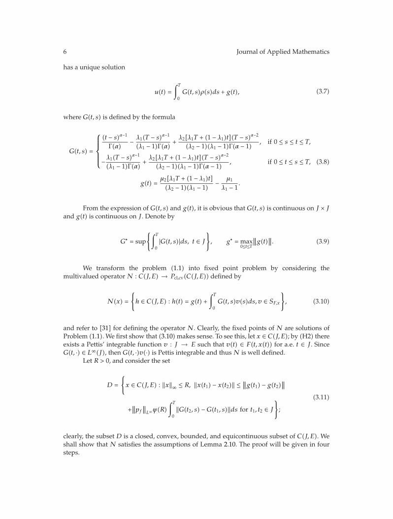
6 Journal of Applied Mathematics
has a unique solution
u(t) =∫T
0G(t, s)ρ(s)ds + g(t), (3.7)
where G(t, s) is defined by the formula
G(t, s) =
⎧⎪⎪⎪⎨
⎪⎪⎪⎩
(t − s)α−1
Γ(α)− λ1(T − s)α−1
(λ1 − 1)Γ(α)+λ2[λ1T + (1 − λ1)t](T − s)α−2
(λ2 − 1)(λ1 − 1)Γ(α − 1), if 0 ≤ s ≤ t ≤ T,
−λ1(T − s)α−1
(λ1 − 1)Γ(α)+λ2[λ1T + (1 − λ1)t](T − s)α−2
(λ2 − 1)(λ1 − 1)Γ(α − 1), if 0 ≤ t ≤ s ≤ T,
g(t) =μ2[λ1T + (1 − λ1)t](λ2 − 1)(λ1 − 1)
− μ1
λ1 − 1.
(3.8)
From the expression of G(t, s) and g(t), it is obvious that G(t, s) is continuous on J × Jand g(t) is continuous on J . Denote by
G∗ = sup
{∫T
0|G(t, s)|ds, t ∈ J
}
, g∗ = max0≤t≤T
∥∥g(t)∥∥. (3.9)
We transform the problem (1.1) into fixed point problem by considering themultivalued operator N : C(J, E) → Pcl,cv(C(J, E)) defined by
N(x) =
{
h ∈ C(J, E) : h(t) = g(t) +∫T
0G(t, s)v(s)ds, v ∈ SF,x
}
, (3.10)
and refer to [31] for defining the operator N. Clearly, the fixed points of N are solutions ofProblem (1.1). We first show that (3.10) makes sense. To see this, let x ∈ C(J, E); by (H2) thereexists a Pettis’ integrable function v : J → E such that v(t) ∈ F(t, x(t)) for a.e. t ∈ J . SinceG(t, ·) ∈ L∞(J), then G(t, ·)v(·) is Pettis integrable and thus N is well defined.
Let R > 0, and consider the set
D =
{
x ∈ C(J, E) : ‖x‖∞ ≤ R, ‖x(t1) − x(t2)‖ ≤ ∥∥g(t1) − g(t2)∥∥
+∥∥pf∥∥L∞ψ(R)
∫T
0‖G(t2, s) −G(t1, s)‖ds for t1, t2 ∈ J
}
;
(3.11)
clearly, the subset D is a closed, convex, bounded, and equicontinuous subset of C(J, E). Weshall show that N satisfies the assumptions of Lemma 2.10. The proof will be given in foursteps.

Journal of Applied Mathematics 7
Step 1. We will show that the operator N(x) is convex for each x ∈ D.Indeed, if h1 and h2 belong to N(x), then there exists Pettis’ integrable functions v1(t),
v2(t) ∈ F(t, x(t)) such that, for all t ∈ J , we have
hi(t) = g(t) +∫T
0G(t, s)vi(s)ds, i = 1, 2. (3.12)
Let 0 ≤ d ≤ 1. Then, for each t ∈ J , we have
[dh1 + (1 − d)h2](t) = g(t) +∫T
0G(t, s)[dv1(s) + (1 − d)v2(s)]ds. (3.13)
Since F has convex values, (dv1 + (1 − d)v2)(t) ∈ F(t, y) and we have dh1 + (1 − d)h2 ∈ N(x).Step 2. We will show that the operator N maps D into D.To see this, take u ∈ ND. Then there exists x ∈ D with u ∈ N(x) and there exists
a Pettis integrable function v : J → E with v(t) ∈ F(t, x(t)) for a.e. t ∈ J . Without loss ofgenerality, we assume u(s)/= 0 for all s ∈ J . Then, there exists ϕs ∈ E∗ with ‖ϕs‖ = 1 andϕs(u(s)) = ‖u(s)‖. Hence, for each fixed t ∈ J , we have
‖u(t)‖ = ϕt(u(t)) = ϕt
(
g(t) +∫T
0G(t, s)v(s)ds
)
≤ ϕt
(g(t))+ ϕt
(∫T
0G(t, s)v(s)ds
)
≤ ∥∥g(t)∥∥ +∫T
0‖G(t, s)‖ϕt(v(s))ds
≤ g∗ +G∗ψ(‖x‖∞)∥∥pf∥∥L∞ .
(3.14)
Therefore, by (H5), we have
‖u‖∞ ≤ g∗ +∥∥pf∥∥L∞G
∗ψ(‖R‖∞) ≤ R. (3.15)
Next suppose u ∈ ND and τ1, τ2 ∈ J , with τ1 < τ2 so that u(τ2) − u(τ1)/= 0. Then, thereexists ϕ ∈ E∗ such that ‖u(τ2) − u(τ1)‖ = ϕ(u(τ2) − u(τ1)). Hence,
‖u(τ2) − u(τ1)‖ = ϕ
(
g(t2) − g(t1) +∫T
0[G(τ2, s) −G(τ1, s)] · v(s)ds
)
≤ ϕ(g(t2) − g(t1)
)+ ϕ
(∫T
0[G(τ2, s) −G(τ1, s)] · v(s)ds
)
≤ ∥∥g(t2) − g(t1)∥∥ +∫T
0‖G(τ2, s) −G(τ1, s)‖·‖v(s)‖ds
≤ ∥∥g(t2) − g(t1)∥∥ + ψ(R)
∥∥pf∥∥L∞
∫T
0‖G(τ2, s) −G(τ1, s)‖ds;
(3.16)
this means that u ∈ D.
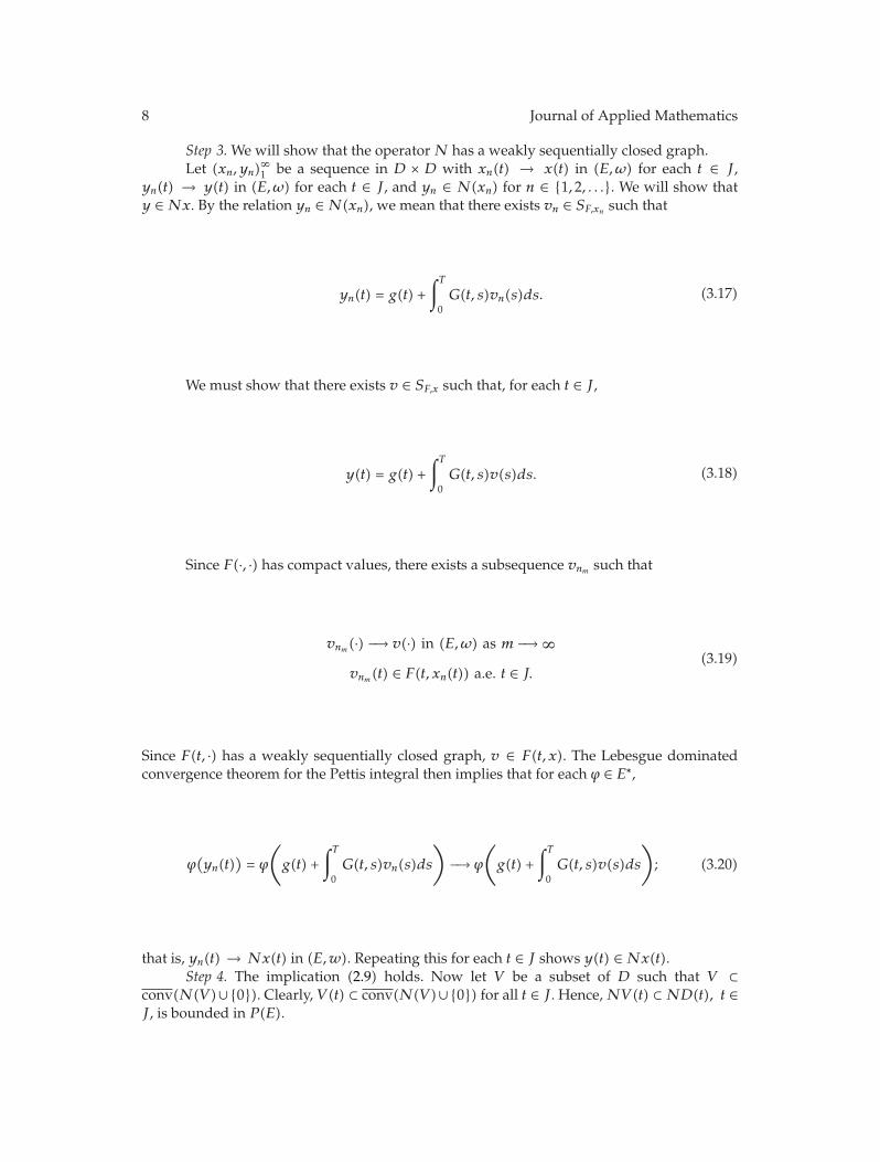
8 Journal of Applied Mathematics
Step 3. We will show that the operator N has a weakly sequentially closed graph.Let (xn, yn)
∞1 be a sequence in D × D with xn(t) → x(t) in (E,ω) for each t ∈ J ,
yn(t) → y(t) in (E,ω) for each t ∈ J , and yn ∈ N(xn) for n ∈ {1, 2, . . .}. We will show thaty ∈ Nx. By the relation yn ∈ N(xn), we mean that there exists vn ∈ SF,xn such that
yn(t) = g(t) +∫T
0G(t, s)vn(s)ds. (3.17)
We must show that there exists v ∈ SF,x such that, for each t ∈ J ,
y(t) = g(t) +∫T
0G(t, s)v(s)ds. (3.18)
Since F(·, ·) has compact values, there exists a subsequence vnm such that
vnm(·) −→ v(·) in (E,ω) as m −→ ∞vnm(t) ∈ F(t, xn(t)) a.e. t ∈ J.
(3.19)
Since F(t, ·) has a weakly sequentially closed graph, v ∈ F(t, x). The Lebesgue dominatedconvergence theorem for the Pettis integral then implies that for each ϕ ∈ E∗,
ϕ(yn(t)
)= ϕ
(
g(t) +∫T
0G(t, s)vn(s)ds
)
−→ ϕ
(
g(t) +∫T
0G(t, s)v(s)ds
)
; (3.20)
that is, yn(t) → Nx(t) in (E,w). Repeating this for each t ∈ J shows y(t) ∈ Nx(t).Step 4. The implication (2.9) holds. Now let V be a subset of D such that V ⊂
conv(N(V )∪{0}). Clearly, V (t) ⊂ conv(N(V )∪{0}) for all t ∈ J . Hence, NV (t) ⊂ ND(t), t ∈J , is bounded in P(E).

Journal of Applied Mathematics 9
Since function g is continuous on J , the set {g(t), t ∈ J} ⊂ E is compact, so β(g(t)) = 0.By assumption (H4) and the properties of the measure β, we have for each t ∈ J
β(N(V )(t)) = β
{
g(t) +∫T
0G(t, s)v(s)ds : v ∈ SF,x, x ∈ V, t ∈ J
}
≤ β{g(t) : t ∈ J
}+ β
{∫T
0G(t, s)v(s)ds : v ∈ SF,x, x ∈ V, t ∈ J
}
≤ β
{∫T
0G(t, s)v(s)ds : v(t) ∈ F(t, x(t)), x ∈ V, t ∈ J
}
≤∫T
0‖G(t, s)‖ · pf(s) · β(V (s))ds
≤ ∥∥pf∥∥L∞ ·∫T
0‖G(t, s)‖ · β(V (s))ds
≤ ∥∥pf∥∥L∞ ·G∗ ·
∫T
0β(V (s))ds,
(3.21)
which gives
‖v‖∞ ≤ ∥∥pf∥∥L∞ · ‖v‖∞ ·G∗. (3.22)
This means that
‖v‖∞ ·[1 − ∥∥pf
∥∥L∞ ·G∗
]≤ 0. (3.23)
By (3.5) it follows that ‖v‖∞ = 0; that is, v = 0 for each t ∈ J , and then V is relatively weaklycompact in E. In view of Lemma 2.10, we deduce that N has a fixed point which is obviouslya solution of Problem (1.1). This completes the proof.
In the sequel we present an example which illustrates Theorem 3.2.
4. An Example
Example 4.1. We consider the following partial hyperbolic fractional differential inclusion ofthe form
(cDαun)(t) ∈ 17et+13
(1 + |un(t)|), t ∈ J := [0, T], 1 < α ≤ 2,
u(0) = λ1u(T) + μ1, u′(0) = λ2u′(T) + μ2,
(4.1)
Set T = 1, λ1 = λ2 = −1, μ1 = μ2 = 0, then g(t) = 0. So g∗ = 0.

10 Journal of Applied Mathematics
Let
E = l1 =
{
u = (u1, u2, . . . , un, . . .) :∞∑
n=1
|un| < ∞}
(4.2)
with the norm
‖u‖E =∞∑
n=1
|un|. (4.3)
Set
u = (u1, u2, . . . , un, . . .), f =(f1, f2, . . . , fn, . . .
),
fn(t, un) =1
7et+13(1 + |un|), t ∈ J.
(4.4)
For each un ∈ R and t ∈ J , we have
∣∣fn(t, un)∣∣ ≤ 1
7et+13(1 + |un|). (4.5)
Hence conditions (H1), (H2), and (H3) hold with pf(t) = 1/(7et+13), t ∈ J , and ψ(u) =1 + u, u ∈ [0,∞). For any bounded set D ⊂ l1, we have
β(F(t,D)) ≤ 17et+13
· β(D), ∀t ∈ J. (4.6)
Hence (H4) is satisfied. From (3.8), we have
G(t, s) =
⎧⎪⎪⎪⎨
⎪⎪⎪⎩
(t − s)α−1
Γ(α)− (1 − s)α−1
2Γ(α)+(1 − 2t)(1 − s)α−2
4Γ(α − 1), if 0 ≤ s ≤ t ≤ 1,
− (1 − s)α−1
2Γ(α)+(1 − 2t)(1 − s)α−2
4Γ(α − 1), if 0 ≤ t ≤ s ≤ 1.
(4.7)

Journal of Applied Mathematics 11
So, we get
∫1
0G(t, s)ds =
∫ t
0G(t, s)ds +
∫1
t
G(t, s)ds
=∫ t
0
[(t − s)α−1
Γ(α)− (1 − s)α−1
2Γ(α)+(1 − 2t)(1 − s)α−2
4Γ(α − 1)
]
ds
+∫1
t
[
− (1 − s)α−1
2Γ(α)+(1 − 2t)(1 − s)α−2
4Γ(α − 1)
]
ds
=4tα − 2
4Γ(α + 1)+
1 − 2t4Γ(α)
.
(4.8)
A simple computation gives
G∗ <1
4Γ(α)+
12Γ(α + 1)
:= Aα. (4.9)
We shall check that condition (3.5) is satisfied. Indeed
∥∥p∥∥L∞G
∗ <1
7e13Aα < 1, (4.10)
which is satisfied for some α ∈ (1, 2], and (H5) is satisfied for R > Aα/(7e13 − Aα). Then byTheorem 3.2, the problem (4.1) has at least one solution on J for values of α satisfying (4.10).
Acknowledgments
The first author’s work was supported by NNSF of China (11161027), NNSF of China(10901075), and the Key Project of Chinese Ministry of Education (210226). The authors aregrateful to the referees for their comments according to which the paper has been revised.
References
[1] R. Hilfer, Applications of Fractional Calculus in Physics, World Scientific, Singapore, 2000.[2] J. Sabatier, O. P. Agrawal, and J. A. Tenreiro Machado, Advances in Fractional Calculus, Springer, 2007.[3] A. A. Kilbas, H. H. Srivastava, and J. J. Trujillo, Theory and Applications of Fractional Differential
Equations, Elsevier Science B.V., Amsterdam, The Netherlands, 2006.[4] V. Lakshmikantham, S. Leela, and J. V. Devi, Theory of Fractional Dynamic Systems, Cambridge Scientific
Publishers, Cambridge, UK, 2009.[5] K. S. Miller and B. Ross, An Introduction to the Fractional Calculus and Fractional Differential Equations,
John Wiley & Sons, New York, NY, USA, 1993.[6] K. B. Oldham and J. Spanier, The Fractional Calculus, Academic Press, New York, NY, USA, 1974.[7] I. Podlubny, Fractional Differential Equations, Mathematics in Science and Engineering, Academic
Press, New York, NY, USA, 1999.[8] S. G. Samko, A. A. Kilbas, and O. I. Marichev, Fractional Integrals and Derivatives, Theory and
Applications, Gordon and Breach Science Publishers, Yverdon, Switzerland, 1993.

12 Journal of Applied Mathematics
[9] R. P. Agarwal, M. Benchohra, and S. Hamani, “Boundary value problems for fractional differentialequations,” Advanced Studies in Contemporary Mathematics, vol. 16, pp. 181–196, 2008.
[10] B. Ahmad and J. J. Nieto, “Existence of solutions for nonlocal boundary value problems of higher-order nonlinear fractional differential equations,” Abstract and Applied Analysis, vol. 2009, Article ID494720, 9 pages, 2009.
[11] Z. Bai and H. Lu, “Positive solutions for boundary value problem of nonlinear fractional differentialequation,” Journal of Mathematical Analysis and Applications, vol. 311, no. 2, pp. 495–505, 2005.
[12] M. El-Shahed and J. J. Nieto, “Nontrivial solutions for a nonlinear multi-point boundary valueproblem of fractional order,” Computers &Mathematics with Applications, vol. 59, no. 11, pp. 3438–3443,2010.
[13] C. F. Li, X. N. Luo, and Y. Zhou, “Existence of positive solutions of the boundary value problem fornonlinear fractional differential equations,” Computers & Mathematics with Applications, vol. 59, no. 3,pp. 1363–1375, 2010.
[14] F. Jiao and Y. Zhou, “Existence of solutions for a class of fractional boundary value problems viacritical point theory,” Computers & Mathematics with Applications, vol. 62, no. 3, pp. 1181–1199, 2011.
[15] J. Wang and Y. Zhou, “Analysis of nonlinear fractional control systems in Banach spaces,” NonlinearAnalysis. Theory, Methods & Applications A, vol. 74, no. 17, pp. 5929–5942, 2011.
[16] G. Wang, B. Ahmad, and L. Zhang, “Impulsive anti-periodic boundary value problem for nonlineardifferential equations of fractional order,” Nonlinear Analysis. Theory, Methods & Applications A, vol.74, no. 3, pp. 792–804, 2011.
[17] W.-X. Zhou and Y.-D. Chu, “Existence of solutions for fractional differential equations with multi-point boundary conditions,” Communications in Nonlinear Science and Numerical Simulation, vol. 17,no. 3, pp. 1142–1148, 2012.
[18] W. Zhou, Y. Chang, and H. Liu, “Weak solutions for nonlinear fractional dif-ferential equations inBanach spaces,” Discrete Dynamics in Nature and Society, vol. 2012, Article ID 527969, 13 pages, 2012.
[19] J. Banas and K. Goebel, Measures of Noncompactness in Banach Spaces, vol. 60, Marcel Dekker, NewYork, NY, USA, 1980.
[20] J. Banas and K. Sadarangani, “On some measures of noncompactness in the space of continuousfunctions,” Nonlinear Analysis. Theory, Methods & Applications A, vol. 68, no. 2, pp. 377–383, 2008.
[21] D. Guo, V. Lakshmikantham, and X. Liu, Nonlinear Integral Equations in Abstract Spaces, vol. 373 ofMathematics and its Applications, Kluwer Academic, Dordrecht, The Netherlands, 1996.
[22] S. Krzyska and I. Kubiaczyk, “On bounded pseudo and weak solutions of a nonlinear differentialequation in Banach spaces,” Demonstratio Mathematica, vol. 32, no. 2, pp. 323–330, 1999.
[23] V. Lakshmikantham and S. Leela, Nonlinear Differential Equations in Abstract Spaces, vol. 2, PergamonPress, New York, NY, USA, 1981.
[24] H. Monch, “Boundary value problems for nonlinear ordinary differential equations of second orderin Banach spaces,” Nonlinear Analysis, vol. 4, no. 5, pp. 985–999, 1980.
[25] D. O’Regan, “Fixed-point theory for weakly sequentially continuous mappings,” Mathematical andComputer Modelling, vol. 27, no. 5, pp. 1–14, 1998.
[26] D. O’Regan, “Weak solutions of ordinary differential equations in Banach spaces,” AppliedMathematics Letters, vol. 12, no. 1, pp. 101–105, 1999.
[27] S. Szufla, “On the application of measure of noncompactness to existence theorems,” Rendiconti delSeminario Matematico della Universita di Padova, vol. 75, pp. 1–14, 1986.
[28] S. Szufla and A. Szukała, “Existence theorems for weak solutions of nth order differential equationsin Banach spaces,” Functiones et Approximatio Commentarii Mathematici, vol. 26, pp. 313–319, 1998,Dedicated to Julian Musielak.
[29] A. Ouahab, “Some results for fractional boundary value problem of differential inclusions,” NonlinearAnalysis. Theory, Methods & Applications A, vol. 69, no. 11, pp. 3877–3896, 2008.
[30] Y.-K. Chang and J. J. Nieto, “Some new existence results for fractional differential inclusions withboundary conditions,” Mathematical and Computer Modelling, vol. 49, no. 3-4, pp. 605–609, 2009.
[31] B. Ahmad, “New results for boundary value problems of nonlinear fractional differential equationswith non-separated boundary conditions,” Acta Mathematica Vietnamica, vol. 36, pp. 659–668, 2011.
[32] B. Ahmad, J. J. Nieto, and A. Alsaedi, “Existence and uniqueness of solutions for nonlinear fractionaldifferential equations with non-separated type integral boundary conditions,” Acta MathematicaScientia B, vol. 31, no. 6, pp. 2122–2130, 2011.
[33] B. Ahmad and S. K. Ntouyas, “Nonlinear fractional differential inclusions with anti-periodictypeintegral boundary conditions,” Discussiones Mathematicae Differential Inclusions, Control andOptimization. In press.

Journal of Applied Mathematics 13
[34] J. Henderson and A. Ouahab, “Impulsive differential inclusions with fractional order,” Computers &Mathematics with Applications, vol. 59, no. 3, pp. 1191–1226, 2010.
[35] J.-P. Aubin and A. Cellina, Differential Inclusions, vol. 264, Springer, New York, NY, USA, 1984.[36] J.-P. Aubin and H. Frankowska, Set-Valued Analysis, vol. 2, Birkhauser, Boston, Mass, USA, 1990.[37] K. Deimling, Multivalued Differential Equations, vol. 1, Walter De Gruyter, New York, NY, USA, 1992.[38] S. Hu and N. S. Papageorgiou, Handbook of Multivalued Analysis, Theory, vol. 1, Kluwer Academic,
Dordrecht, The Netherlands, 1997.[39] M. Kisielewicz, Differential Inclusions and Optimal Control, Kluwer Academic, Dordrecht, The
Netherlands, 1991.[40] H. Covitz and S. B. Nadler Jr., “Multi-valued contraction mappings in generalized metric spaces,”
Israel Journal of Mathematics, vol. 8, pp. 5–11, 1970.[41] B. J. Pettis, “On integration in vector spaces,” Transactions of the American Mathematical Society, vol. 44,
no. 2, pp. 277–304, 1938.[42] F. S. De Blasi, “On a property of the unit sphere in a Banach space,” Bulletin Mathematique de la Societe
des Sciences Mathematiques de Roumanie, vol. 21, pp. 259–262, 1977.[43] H. A. H. Salem, A. M. A. El-Sayed, and O. L. Moustafa, “A note on the fractional calculus in Banach
spaces,” Studia Scientiarum Mathematicarum Hungarica, vol. 42, no. 2, pp. 115–130, 2005.

Hindawi Publishing CorporationJournal of Applied MathematicsVolume 2012, Article ID 804032, 18 pagesdoi:10.1155/2012/804032
Research ArticleWell-Posedness by Perturbations forVariational-Hemivariational Inequalities
Shu Lv,1 Yi-bin Xiao,1 Zhi-bin Liu,2, 3 and Xue-song Li4
1 School of Mathematical Sciences, University of Electronic Science and Technology of China,Sichuan, Chengdu 610054, China
2 Department of Applied Mathematics, Southwest Petroleum University, Chengdu 610500, China3 State Key Laboratory of Oil and Gas Reservoir and Exploitation, Chengdu 610500, China4 Department of Mathematics, Sichuan University, Sichuan, Chengdu 610064, China
Correspondence should be addressed to Yi-bin Xiao, [email protected]
Received 18 January 2012; Accepted 4 July 2012
Academic Editor: Hong-Kun Xu
Copyright q 2012 Shu Lv et al. This is an open access article distributed under the CreativeCommons Attribution License, which permits unrestricted use, distribution, and reproduction inany medium, provided the original work is properly cited.
We generalize the concept of well-posedness by perturbations for optimization problem to aclass of variational-hemivariational inequalities. We establish some metric characterizations ofthe well-posedness by perturbations for the variational-hemivariational inequality and provetheir equivalence between the well-posedness by perturbations for the variational-hemivariationalinequality and the well-posedness by perturbations for the corresponding inclusion problem.
1. Introduction and Preliminaries
The concept well-posedness is important in both theory and methodology for optimizationproblems. An initial, already classical concept of well-posedness for unconstrained optimiza-tion problem is due to Tykhonov in [1]. Let f : V → R∪ {+∞} be a real-valued functional onBanach space V . The problem of minimizing f on V is said to be well-posed if there exists aunique minimizer, and every minimizing sequence converges to the unique minimizer. Soonafter, Levitin and Polyak [2] generalized the Tykhonov well-posedness to the constrainedoptimization problem, which has been known as the Levitin-Polyak well-posedness. It isclear that the concept of well-posedness is motivated by the numerical methods producingoptimizing sequences for optimization problems. Unfortunately, these concepts generallycannot establish appropriate continuous dependence of the solution on the data. In turn, theyare not suitable for the numerical methods when the objective functional f is approximated

2 Journal of Applied Mathematics
by a family or a sequence of functionals. For this reason, another important concept of well-posedness for optimization problem, which is called the well-posedness by perturbationsor extended well-posedness, has been introduced and studied by [3–6]. Also, many othernotions of well-posedness have been introduced and studied for optimization problem. Fordetails, we refer to [7] and the reference therein.
The concept well-posedness also has been generalized to other related problems,especially to the variational inequality problem. Lucchetti and Patrone [8] first introducedthe well-posedness for a variational inequality, which can be regarded as an extensionof the Tykhonov well-posedness of optimization problem. Since then, many authors weredevoted to generalizing the concept of well-posedness for the optimization problem tovarious variational inequalities. In [9], Huang et al. introduced several types of (generalized)Levitin-Polyak well-posednesses for a variational inequality problem with abstract andfunctional constraint and gave some criteria, characterizations, and their relations forthese types of well-posednesses. Recently, Fang et al. [10] generalized the concept ofwell-posedness by perturbations, introduced by Zelezzi for a minimization problem, to ageneralized mixed variational inequality problem in Banach space. They established somemetric characterizations of well-posedness by perturbations and discussed its links withwell-posedness by perturbations of corresponding inclusion problem and the well-posednessby perturbations of corresponding fixed point problem. Also they derived some conditionsunder which the well-posedness by perturbations of the mixed variational inequality isequivalent to the existence and uniqueness of its solution. For further more results on thewell-posedness of variational inequalities, we refer to [8–15] and the references therein.
When the corresponding energy functions are not convex, the mathematical modeldescribing many important phenomena arising in mechanics and engineering is no longervariational inequality but a new type of inequality problem that is called hemivariationalinequality, which was first introduced by Panagiotopoulos [16] as a generalization of vari-ational inequality. A more generalized variational formulation which is called variational-hemivariational inequality is presented to model the problems subject to constraints becausethe setting of hemivariational inequalities cannot incorporate the indicator function of aconvex closed subset. Due to the fact that the potential is neither convex nor smoothgenerally, the hemivariational inequalities have been proved very efficient to describe avariety of mechanical problems using the generalized gradient of Clarke for nonconvex andnondifferentiable functions [17], such as unilateral contact problems in nonlinear elasticity,obstacles problems, and adhesive grasping in robotics (see, e.g., [18–20]). So, in recentyears all kinds of hemivariational inequalities have been studied [21–30] and the studyof hemivariational inequalities has emerged as a new and interesting branch of appliedmathematics. However, there are very few researchers extending the well-posedness tohemivariational inequality. In 1995, Goeleven and Mentagui [23] first defined the well-posedness for hemivariational inequalities. Recently, Xiao et al. [31] generalized theconcept of well-posedness to hemivariational inequalities. They established some metriccharacterizations of the well-posed hemivariational inequality, derived some conditionsunder which the hemivariational inequality is strongly well-posed in the generalized sense,and proved the equivalence between the well-posedness of hemivariational inequality andthe well-posedness of a corresponding inclusion problem. Moreover, Xiao and Huang [32]studied the well-posedness of variational-hemivariational inequalities and generalized somerelated results.
In the present paper, we generalize the well-posedness by perturbations for optimiza-tion problem to a class of variational-hemivariational inequality. We establish some metric

Journal of Applied Mathematics 3
characterizations of the well-posedness by perturbations for variational-hemivariationalinequality and prove the equivalence between the well-posedness by perturbations forthe variational-hemivariational inequality and the well-posedness by perturbations for thecorresponding inclusion problem.
We suppose in what follows that V is a real reflexive Banach space with its dual V ∗,and 〈·, ·〉 is the duality between V and V ∗. We denote the norms of Banach space V and V ∗
by ‖ · ‖V and ‖ · ‖V ∗ , respectively. Let A : V → V ∗ be a mapping, let J : V → R be a locallyLipschitz functional, let G : V → R ∪ {+∞} be a proper, convex, and lower semicontinuousfunctional, and let f ∈ V ∗ be some given element. Denote by dom G the domain of functionalG, that is,
dom G = {u ∈ V : G(u) < +∞}. (1.1)
The functional G is called proper if its domain is nonempty. The variational-hemivariationalinequality associated with (A, f, J, G) is specified as follows:
VHVI(A, f, J, G
):
find u ∈ dom G such that 〈A(u), v − u〉 + J◦(u, v − u) +G(v) −G(u) ≥ ⟨f, v − u
⟩, ∀v ∈ V,
(1.2)
where J◦(u, v) denotes the generalized directional derivative in the sense of Clarke of a locallyLipschitz functional J at u in the direction v (see [17]) given by
J◦(u, v) = lim supw→u λ↓0
J(w + λv) − J(w)λ
. (1.3)
The variational-hemivariational inequality which includes many problems as special caseshas been studied intensively. Some special cases of VHVI(A, f, J, G) are as follows:
(i) if G = 0, then VHVI(A, f, J, G) reduces to hemivariational inequality:
HVI(A, f, J
):
find u ∈ V such that 〈A(u), v − u〉 + J◦(u, v − u) ≥ ⟨f, v − u
⟩, ∀v ∈ V,
(1.4)
(ii) if J = 0, then VHVI(A, f, J, G) is equivalent to the following mixed variationalinequality:
MVI(A, f,G
):
find u ∈ dom G such that 〈A(u), v − u〉 +G(v) −G(u) ≥ ⟨f, v − u
⟩, ∀v ∈ V,
(1.5)
(iii) if A = 0, J = 0 and f = 0, then VHVI(A, f, J, G) reduces to the global minimizationproblem:
MP(G) : minu∈V
G(u). (1.6)

4 Journal of Applied Mathematics
Let ∂G(u) : V → 2V∗ \{∅} and ∂J(u) : V → 2V
∗ \{∅} denote the subgradient of convexfunctional G in the sense of convex analysis (see [33]) and the Clarke’s generalized gradientof locally Lipschitz functional J (see [17]), respectively, that is,
∂G(u) = {u∗ ∈ V ∗ : G(v) −G(u) ≥ 〈u∗, v − u〉, ∀v ∈ V },
∂J(u) = {ω ∈ V ∗ : J◦(u, v) ≥ 〈ω, v〉, ∀v ∈ V }.(1.7)
About the subgradient in the sense of convex analysis, the Clarke’s generalized directionalderivative and the Clarke’s generalized gradient, we have the following basic properties (see,e.g., [17, 19, 33, 34]).
Proposition 1.1. Let V be a Banach space and G : V → R ∪ {+∞} a convex and proper functional.Then one has the following properties of ∂G:
(i) ∂G(u) is convex and weak∗-closed;
(ii) if G is continuous at u ∈ dom G, then ∂G(u) is nonempty, convex, bounded, and weak∗-compact;
(iii) if G is Gateaux differentiable at u ∈ dom G, then ∂G(u) = {DG(u)}, whereDG(u) is theGateaux derivative of G at u.
Proposition 1.2. Let V be a Banach space, and let G1, G2 : V → R ∪ {+∞} be two convexfunctionals. If there is a point u0 ∈ dom G1 ∩ dom G2 at which G1 is continuous, then the followingequation holds:
∂(G1 +G2)(u) = ∂G1(u) + ∂G2(u), ∀u ∈ V. (1.8)
Proposition 1.3. Let V be a Banach space, u, v ∈ V , and let J be a locally Lipschitz functional definedon V . Then
(1) the function v �→ J◦(u, v) is finite, positively homogeneous, subadditive, and then convexon V ,
(2) J◦(u, v) is upper semicontinuous as a function of (u, v), as a function of v alone, isLipschitz continuous on V ,
(3) J◦(u,−v) = (−J)◦(u, v),(4) ∂J(u) is a nonempty, convex, bounded, and weak∗-compact subset of V ∗,
(5) for every v ∈ V , one has
J◦(u, v) = max{〈ξ, v〉 : ξ ∈ ∂J(u)
}. (1.9)
Suppose that L is a parametric normed space with norm ‖ · ‖L, P ⊂ L is a closed ballwith positive radius, and p∗ ∈ P is a given point. We denote the perturbed mappings of A,J , G as A : P × V → V ∗ and J , G : P × V → R, respectively, which have the property that

Journal of Applied Mathematics 5
for any p ∈ P , J(p, ·) is a locally Lipschitz functional in V , G(p, ·) is proper, convex, and lowersemicontinuous in V , and
A(p∗, ·) = A(·), J
(p∗, ·) = J(·), G
(p∗, ·) = G(·). (1.10)
Then the perturbed Clarke’s generalized directional derivative J◦2 (p, ·) : V × V → R and theperturbed Clarke’s generalized gradient ∂2J(p, ·) : V → 2V
∗corresponding to the perturbed
locally Lipschitz functional J are, respectively, specified as
J◦2(p, ·)(u, v) = lim sup
w→u λ↓0
J(p,w + λv
) − J(p,w
)
λ,
∂2J(p, u
)={ω ∈ V ∗ : J◦2
(p, ·)(u, v) ≥ 〈ω, v〉, ∀v ∈ V
}.
(1.11)
The perturbed subgradient ∂2G(p, ·) : dom G → 2V∗
corresponding to the perturbed convexfunctional G is
∂2G(p, u
)={u∗ ∈ V ∗ : G
(p, v
) − G(p, u
) ≥ 〈u∗, v − u〉, ∀v ∈ V}. (1.12)
Based on the above-perturbed mappings, the perturbed problem of VHVI(A, f, J, G) is givenby
VHVIp(A, f, J, G
):
find u ∈ dom G(p, ·) such that
⟨A(p, u
) − f, v − u⟩+ J◦2
(p, ·)(u, v − u) + G
(p, v
)
− G(p, u
) ≥ 0, ∀v ∈ V.
(1.13)
In the sequel, we recall some important definitions and useful results.
Definition 1.4 (see [35]). Let S be a nonempty subsets of V . The measure of noncompactnessμ of the set S is defined by
μ(S) = inf
{
ε > 0 : S ⊂n⋃
i=1
Si,diam(Si) < ε, i = 1, 2, . . . , n
}
, (1.14)
where diam(Si) means the diameter of set Si.
Definition 1.5 (see [35]). Let A and B be two given subsets of V . The excess of A over B isdefined by
e(A,B) = supa∈A
d(a, B), (1.15)

6 Journal of Applied Mathematics
where d(·, B) is the distance function generated by B, that is,
d(x, B) = infb∈B
‖a − b‖V , x ∈ V. (1.16)
The Hausdorff metric H(·, ·) between A and B is defined by
H(A,B) = max{e(A,B), e(B,A)}. (1.17)
Let {An} be a sequence of nonempty subset of V . One says that An converges to A in thesense of Hausdorff metric if H(An,A) → 0. It is easy to see that e(An,A) → 0 if and only ifd(an,A) → 0 for all selection an ∈ An. For more details on this topic, the reader should referto [35]. The following theorem is crucial to our main results.
Theorem 1.6 (see [36]). Let C ⊂ V be nonempty, closed, and convex, let C∗ ⊂ V ∗ be nonempty,closed, convex, and bounded, let ϕ : V → R be proper, convex, and lower semicontinuous, and lety ∈ C be arbitrary. Assume that, for each x ∈ C, there exists x∗(x) ∈ C∗ such that
⟨x∗(x), x − y
⟩ ≥ ϕ(y) − ϕ(x). (1.18)
Then, there exists y∗ ∈ C∗ such that
⟨y∗, x − y
⟩ ≥ ϕ(y) − ϕ(x), ∀x ∈ C. (1.19)
2. Well-Posedness by Perturbations of VHVI(A, f, J, G) withMetric Characterizations
In this section, we generalize the concept of well-posedness by perturbations to the vari-ational-hemivariational inequality VHVI(A, f, J, G) and establish its metric characteriza-tions.
Definition 2.1. Let {pn} ⊂ P with pn → p∗. A sequence {un} ⊂ V is said to be an approximatingsequence corresponding to {pn} for VHVI(A, f, J, G) if there exists a nonnegative sequence{εn} with εn → 0 as n → ∞ such that un ∈ dom G(pn, ·) and
⟨A(pn, un
) − f, v − un
⟩+ J◦2
(pn, ·
)(un, v − un) + G
(pn, v
) − G(pn, un
)
≥ −εn‖v − un‖V , ∀v ∈ V.
(2.1)
Definition 2.2. VHVI(A, f, J, G) is said to be strongly (resp., weakly) well-posed by pertur-bations if VHVI(A, f, J, G) has a unique solution in V , and for any {pn} ⊂ P with pn → p∗,every approximating sequence corresponding to {pn} converges strongly (resp., weakly) tothe unique solution.
Remark 2.3. Strong well-posedness by perturbations implies weak well-posedness by pertur-bations, but the converse is not true in general.

Journal of Applied Mathematics 7
Definition 2.4. VHVI(A, f, J, G) is said to be strongly (resp., weakly) well-posed byperturbations in the generalized sense if VHVI(A, f, J, G) has a nonempty solution set S in V ,and for any {pn} ⊂ P with pn → p∗, every approximating sequence corresponding to {pn} hassome subsequence which converges strongly (resp., weakly) to some point of solution set S.
Remark 2.5. Strong well-posedness by perturbations in the generalized sense implies weakwell-posedness by perturbations in the generalized sense, but the converse is not true ingeneral.
To derive the metric characterizations of well-posedness by perturbations forVHVI(A, f, J, G), we define the following approximating solution set of VHVI(A, f, J, G):For any ε > 0,
Ω(ε) =⋃
p∈B(p∗,ε)
{u ∈ dom G
(p, ·) :
⟨A(p, u
) − f, v − u⟩+ J◦2
(p, ·)(u, v − u)
+ G(p, v
) − G(p, u
) ≥ −ε‖v − u‖V , ∀v ∈ V},
(2.2)
where B(p∗, ε) denotes the closed ball centered at p∗ with radius ε. For any ε > 0, u ∈ Ω(ε)and any set K ⊂ Ω(ε), we define the following two functions which are specified as follows:
p(ε, u) = sup{‖v − u‖V : v ∈ Ω(ε)},q(ε,K) = e(Ω(ε), K).
(2.3)
It is easy to see that p(ε, u) is the smallest radius of the closed ball centered at u containingΩ(ε), and q(ε,K) is the excess of approximating solution set Ω(ε) over K.
Based on the two functions p(ε, u) and q(ε,K), we now give some metric characteri-zations of well-posedness by perturbations for the VHVI(A, f, J, G).
Theorem 2.6. VHVI(A, f, J, G) is strongly well-posed by perturbations if and only if there exists asolution u∗ for VHVI(A, f, J, G) and p(ε, u∗) → 0 as ε → 0.
Proof. “Necessity”: suppose that VHVI(A, f, J, G) is strongly well-posed by perturbations.Then Ω(ε)/= ∅ for all ε > 0 since there is a unique solution u∗ belonging to Ω(ε) by the strongwell-posedness by perturbations for VHVI(A, f, J, G). We now need to prove p(ε, u∗) → 0as ε → 0. Assume by contradiction that p(ε, u∗) does not converge to 0 as ε → 0, then thereexist a constant l > 0 and a nonnegative sequence {εn} with εn → 0 such that
p(εn, u∗) > l > 0, ∀n ∈ N. (2.4)
By the definition of function p(ε, u), there exists un ∈ Ω(εn) such that
‖un − u∗‖V > l, ∀n ∈ N. (2.5)

8 Journal of Applied Mathematics
Since un ∈ Ω(εn), there exists some pn ∈ B(p∗, εn) such that
〈A(pn, un
) − f, v − un〉 + J◦2(pn, ·
)(un, v − un) + G
(pn, v
) − G(pn, un
)
≥ −εn‖v − un‖V , ∀v ∈ V, n ∈ N.(2.6)
It is obvious that pn → p∗ as n → ∞ and so {un} is an approximating sequencecorresponding to {pn} for VHVI(A, f, J, G). Therefore, by the strong well-posedness byperturbations for VHVI(A, f, J, G), we can get un → u∗ which is a contradiction to (2.4).
“Sufficiency”: suppose that VHVI(A, f, J, G) has a solution u∗ and p(ε, u∗) → 0 as ε →0. First, we claim that u∗ is a unique solution for VHVI(A, f, J, G). In fact, if VHVI(A, f, J, G)has another solution u with u∗ /= u, it follows from the definition of Ω(ε) that u∗ and u belongto Ω(ε) for all ε > 0, which together with the definition of p(ε, u) implies that
p(ε, u∗) ≥ ‖u − u∗‖V > 0, ∀ε > 0, (2.7)
which is a contradiction to the assumption p(ε, u∗) → 0 as ε → 0. Now, let {pn} ⊂ P withpn → p∗ and {un} be an approximating sequence corresponding to {pn} for VHVI(A, f, J, G).Then there exists a nonnegative sequence {εn} with εn → 0 such that
〈A(pn, un
) − f, v − un〉 + J◦2(pn, ·
)(un, v − un) + G
(pn, v
) − G(pn, un
)
≥ −εn‖v − un‖V , ∀v ∈ V, n ∈ N.(2.8)
Taking δn = ‖pn − p∗‖L and ε′n = max{δn, εn}, it easy to see that ε′n → 0 as n → ∞ andun ∈ Ω(ε′n). Since u∗ is the unique solution for VHVI(A, f, J, G), u∗ also belongs to Ω(ε′n).And so, it follows from the definition of p(ε, u) that
‖un − u∗‖V ≤ p(ε′n, u
∗) −→ 0, as n −→ ∞, (2.9)
which implies that VHVI(A, f, J, G) is strongly well-posed by perturbations. This completesthe proof of Theorem 2.6.
Theorem 2.7. VHVI(A, f, J, G) is strongly well-posed by perturbations in the generalized sense ifand only if the solution set S of VHVI(A, f, J, G) is nonempty and compact, and q(ε, S) → 0 asε → 0.
Proof. “Necessity”: suppose that VHVI(A, f, J, G) is strongly well-posed by perturbations inthe generalized sense. Then VHVI(A, f, J, G) has nonempty solution set S by the definitionof strong well-posedness by perturbations in the generalized sense of VHVI(A, f, J, G).Let {un} be any sequence in S. It is obvious that {un} is an approximating sequencecorresponding to constant sequence {p∗} for VHVI(A, f, J, G). Again by the strong well-posedness by perturbations in the generalized sense of VHVI(A, f, J, G), {un} has asubsequence which converges strongly to some point of S, which implies that the solutionset S of VHVI(A, f, J, G) is compact. Now we show that q(ε, S) → 0 as ε → 0. Assume by

Journal of Applied Mathematics 9
contradiction that q(ε, S) � 0 as ε → 0, then there exist a constant l > 0 and a nonnegativesequence {εn} with εn → 0 and xn ∈ Ω(εn) such that
xn /∈ S + B(0, l), ∀n ∈ N. (2.10)
Since xn ∈ Ω(εn), there exists pn ∈ B(p∗, εn) such that
⟨A(pn, xn
) − f, v − xn
⟩+ J◦2
(pn, ·
)(xn, v − xn) + G
(pn, v
) − G(pn, xn
)
≥ −εn‖v − xn‖V , ∀v ∈ V.
(2.11)
Clearly, pn → p∗ as n → ∞. This together with the above inequality implies that {xn} is anapproximating consequence corresponding to {pn} for VHVI(A, f, J, G). It follows from thestrongly well-posedness by perturbations in the generalized sense for VHVI(A, f, J, G) thatthere is a subsequence {unk} of {un} which converges to some point of S. This is contradictionto (2.10) and so q(ε, S) → 0 as ε → 0.
“Sufficiency”: we suppose that the solution set S of VHVI(A, f, J, G) is nonemptycompact and q(ε, S) → 0 as ε → 0. Let {pn} ⊂ P be any sequence with pn → p∗ and {un} anapproximating sequence corresponding to pn for VHVI(A, f, J, G), which implies that
⟨A(pn, un
) − f, v − un
⟩+ J◦2
(pn, ·
)(un, v − un) + G
(pn, v
) − G(pn, un
)
≥ −εn‖v − un‖V , ∀v ∈ V.
(2.12)
Taking ε′n = max{εn, ‖pn − p∗‖L}, it is easy to see that ε′n → 0 and un ∈ Ω(ε′n). It follows that
d(un, S) ≤ e(Ω(ε′n, S
))= q
(ε′n, S
) −→ 0. (2.13)
Since the solution set S of VHVI(A, f, J, G) is compact, there exists un ∈ S such that
‖un − un‖V = d(un, S) −→ 0. (2.14)
Again from the compactness of solution set S, un has a subsequence {unk} convergingstrongly to some point u ∈ S. It follows from (2.14) that
‖unk − u‖V ≤ ‖unk − unk‖V + ‖unk − u‖V −→ 0, (2.15)
which implies that {unk} converges strongly to u. Thus, VHVI(A, f, J, G) is strongly well-posed by perturbations in the generalized sense. This completes the proof of Theorem 2.7.
The strong well-posedness by perturbations in the generalized sense forVHVI(A, f, J, G) can also be characterized by the behavior of noncompactness measureof its approximating solution set.

10 Journal of Applied Mathematics
Theorem 2.8. Let L be a finite-dimensional space. Suppose that
(i) A(·, ·) : P × V → V ∗, the perturbed mapping of A, is continuous with respect to (p, v),
(ii) G : P × V → R ∪ {+∞}, the perturbed functional of G, is lower semicontinuous withrespect to (p, v) and continuous with respect to p for any given v ∈ V ,
(iii) J : P × V → R, the perturbed functional of J , is locally Lipschitz with respect to v for anyp ∈ P , and its Clarke’s generalized directional derivative J◦2 (p, ·) : P → L(V × V,R) iscontinuous with respect to p.
Then, VHVI(A, f, J, G) is strongly well-posed by perturbations in the generalized sense if andonly if
Ω(ε)/= ∅, ∀ε > 0, μ(Ω(ε)) −→ 0 as ε −→ 0. (2.16)
Proof. From the metric characterization of strongly well-posedness by perturbations in thegeneralized sense for VHVI(A, f, J, G) in Theorem 2.7, we can easily prove the necessity. Infact, since VHVI(A, f, J, G) is strongly well-posed by perturbations in the generalized sense,it follows from Theorem 2.7 that the solution set S of VHVI(A, f, J, G) is nonempty compactand q(ε, S) → 0 as ε → 0. Then, we can easily get from the compactness of S and the factS ⊂ Ω(ε) for all ε > 0 that Ω(ε)/= ∅ for all ε > 0 and
μ(Ω(ε)) ≤ 2H(Ω(ε), S) + μ(S) = 2e(Ω(ε), S) = 2q(ε, S) −→ 0. (2.17)
Now we prove the sufficiency. First, we claim that Ω(ε) is closed for all ε > 0. In fact, let{un} ⊂ Ω(ε) and un → u. Then there exists pn ∈ B(p∗, ε) such that
⟨A(pn, un
) − f, v − un
⟩+ J◦2
(pn, ·
)(un, v − un) + G
(pn, v
) − G(pn, un
)
≥ −ε‖v − un‖V , ∀v ∈ V.
(2.18)
Without loss of generality, we can suppose that pn → p ∈ B(p∗, ε) since L is finitedimensional. By taking lim sup at both sides of above inequality, it follows from theassumptions (i)–(iii) and the upper semicontinuity of J◦2 (p, ·)(u, v) with respect to (u, v) that
⟨A(p, u
) − f, v − u⟩+ J◦2
(p, ·)(u, v − u) + G
(p, v
) − G(p, u
)
≥ lim sup{⟨
A(pn, un
) − f, v − un
⟩+ J◦2
(pn, ·
)(un, v − un) + G
(pn, v
) − G(pn, un
)}
≥ lim sup{−ε‖v − un‖V }= −ε‖v − u‖V .
(2.19)
Thus, u ∈ Ω(ε) and so Ω(ε) is closed.Second, we prove that
S =⋂
ε>0
Ω(ε). (2.20)

Journal of Applied Mathematics 11
It is obvious that S ⊂ ∩ε>0Ω(ε) since the solution set S ⊂ Ω(ε) for all ε > 0. Conversely, letu ∈ ∩ε>0Ω(ε), and let {εn} be a nonnegative sequence with εn → 0 as n → +∞. Then for anyn ∈ N, u ∈ Ω(εn), and so there exists pn ∈ B(p∗, εn) such that
⟨A(pn, u
) − f, v − u⟩+ J◦2
(pn, ·
)(u, v − u) + G
(pn, v
) − G(pn, u
)
≥ −εn‖v − u‖V , ∀v ∈ V.
(2.21)
Since pn ∈ B(p∗, εn) and εn → 0, it is clear that pn → p∗. By letting n → +∞ in the aboveinequality, we get from the continuity of A, J◦2 (p, ·), and G in assumptions that
⟨A(u) − f, v − u
⟩+ J◦(u, v − u) +G(v) −G(u)
=⟨A(p∗, u
) − f, v − u⟩+ J◦2
(p∗, ·)(u, v − u) + G
(p∗, v
) − G(p∗, u
)
≥ lim{−εn‖v − u‖V } = 0.
(2.22)
Thus, u ∈ S and so ∩ε>0Ω(ε) ⊂ S.Now, we suppose that
Ω(ε)/= ∅, ∀ε > 0, μ(Ω(ε)) −→ 0 as ε −→ 0. (2.23)
From the definition of approximating solution set Ω(ε), Ω(ε) is increasing with respect to ε.Then by applying the Kuratowski theorem on page 318 in [35], we have from (2.20) that S isnonempty compact and
q(ε, S) = e(Ω(ε), S) = H(Ω(ε), S) −→ 0 as ε −→ 0. (2.24)
Therefore, by Theorem 2.7, VHVI(A, f, J, G) is strongly well-posed by perturbations in thegeneralized sense.
Example 2.9. Let L be a finite-dimensional space with norm ‖ · ‖L, let P ⊂ L be a closed ball inL, and let p∗ be a given point in P . We supposed that the perturbed mappings A : P×V → V ∗,G, J : P × V → R of the mapping A, G, J are, respectively, specified as follows:
A(p, v
)= expα‖p−p∗‖LA(v), G
(p, v
)= G(v) + β
∥∥p − p∗∥∥L,
J(p, v
)= J(v) + γ
∥∥p − p∗∥∥L,
(2.25)
where α, β, γ are three positive numbers. It is obvious that A is continuous with respect to(p, v) due to the continuity of the mapping A : V → V ∗, and G is lower semicontinuous withrespect to (p, v) and continuous with respect to p for any given v ∈ V because the functionalG : V → R is proper convex and lower semicontinuous. Also, the perturbed functional J islocally Lipschitz with respect to v since J : V → R is locally Lipschitz. Furthermore, it is easy
12 Journal of Applied Mathematics
to check that the perturbed Clarke’s generalized directional derivative corresponding to theperturbed function J can be specified as
J◦2(p, ·)(u, v) = J◦(u, v) = lim sup
w→u λ↓0
J(w + λv) − J(w)λ
, (2.26)
which implies that J◦2 (p, ·) is continuous with respect to p. Thus, the assumptions inTheorem 2.8 are satisfied, and so the VHVI(A, f, J, G) is strongly well-posed by perturbationsin the generalized sense if and only if (2.16) holds.
3. Links with Well-Posedness by Perturbations forCorresponding Inclusion Problem
In this section, we recall some concepts of well-posedness by perturbations for inclusionproblems, which are introduced by Lemaire et al. [4], and investigate the relations betweenthe well-posedness by perturbations for VHVI(A, f, J, G) and the well-posedness byperturbations for the corresponding inclusion problem.
In what follows, we always let F be a set-valued mapping from real reflexive Banachspace V to its dual space V ∗. The inclusion problem associated with mapping F is defined by
IP(F) : find x ∈ V such that 0 ∈ F(x), (3.1)
whose corresponding perturbed problem is specified as
IPp(F) : find x ∈ V such that 0 ∈ F(p, x
), (3.2)
where F : P × V → 2V∗
is the perturbed set-valued mapping such that F(p∗, ·) = F.
Definition 3.1 (see [4]). Let {pn} ⊂ P be a sequence in P with pn → p∗. A sequence {un} ⊂ Vis said to be an approximating sequence corresponding to {pn} for inclusion problem IP(F)if un ∈ dom F(pn, ·) for all n ∈ N and d(0, F(pn, un)) → 0, or equivalently, there exists asequence wn ∈ F(pn, un) such that ‖wn‖V ∗ → 0 as n → ∞.
Definition 3.2 (see [4]). One says that inclusion problem IP(F) is strongly (resp., weakly)well-posed by perturbations if it has a unique solution, and for any {pn} ⊂ P with pn → p∗,every approximating sequence corresponding to {pn} converges strongly (resp., weakly) tothe unique solution of IP(F).
Definition 3.3 (see [4]). One says that inclusion problem IP(F) is strongly (resp., weakly)well-posed by perturbations in the generalized sense if the solution set S of IP(F) isnonempty, and for any {pn} ⊂ P with pn → p∗, every approximating sequence correspondingto {pn} has a subsequence converging strongly (resp., weakly) to some point of solution setS for IP(F).
In order to obtain the relations between the strong (resp., weak) well-posednessby perturbations for variational-hemivariational inequality VHVI(A, f, J, G) and the strong

Journal of Applied Mathematics 13
(resp., weak) well-posedness by perturbations for the corresponding inclusion problem,we first give the following important lemma which establishes the equivalence betweenthe variational-hemivariational inequality VHVI(A, f, J, G) and the corresponding inclusionproblem. Although the lemma is a corollary of Lemma 4.1 in [32] with T = 0, we also giveproof here for its importance and the completeness of our paper.
Lemma 3.4. Let A be a mapping from Banach space V to its dual V ∗, let J : V → R be a locallyLipschitz functional, letG : V → R∪{+∞} be a proper, convex, and lower semicontinuous functional,and let f be a given element in dual space V ∗. Then u ∈ dom G is a solution of VHVI(A, f, J, G) ifand only if u is a solution of the following inclusion problem:
IP(A − f + ∂J + ∂G
): find u ∈ dom G such that Au − f + ∂J(u) + ∂G(u) � 0. (3.3)
Proof. “Sufficiency”: assume that u ∈ dom G is a solution of inclusion problem IP(A − f +∂J + ∂G). Then there exist ω1 ∈ ∂J(u) and ω2 ∈ ∂G(u) such that
Au − f +ω1 +ω2 = 0. (3.4)
By multiplying v − u at both sides of above equation (3.4), we obtain from the definitionsof the Clarke’s generalized gradient for locally Lipschitz functional and the subgradient forconvex functional that
0 =⟨Au − f +ω1 +ω2, v − u
⟩ ≤ ⟨Au − f, v − u
⟩+ J◦(u, v − u)
+G(v) −G(u), ∀v ∈ V,(3.5)
which implies that u ∈ dom G is a solution of VHVI(A, f, J, G).“Necessity”: conversely, suppose that u ∈ dom G is a solution of VHVI(A, f, J, G).
Then,
⟨Au − f, v − u
⟩+ J◦(u, v − u) +G(v) −G(u) ≥ 0, ∀v ∈ V. (3.6)
From the fact that
J◦(u, v − u) = max{〈ω, v − u〉 : ω ∈ ∂J(u)
}, (3.7)
we get that there exists a ω(u, v) ∈ ∂J(u) such that
⟨Au − f, v − u
⟩+ 〈ω(u, v), v − u〉 +G(v) −G(u) ≥ 0, ∀v ∈ V. (3.8)
By virtue of Proposition 1.3, ∂J(u) is a nonempty, convex, and bounded subset in V ∗ whichimplies that {Au − f + ω : ω ∈ ∂J(u)} is nonempty, convex, and bounded in V ∗. Since G :V → R ∪ {+∞} is a proper, convex, and lower semicontinuous functional, it follows from

14 Journal of Applied Mathematics
(3.8) and Theorem 1.6 with ϕ(u) = G(u) that there exists ω(u) ∈ ∂J(u), which is independenton v, such that
⟨Au − f, v − u
⟩+ 〈ω(u), v − u〉 +G(v) −G(u) ≥ 0, ∀v ∈ V. (3.9)
For the sake of simplicity in writing, we denote ω = ω(u). Then by (3.9), we have
G(v) −G(u) ≥ ⟨−Au + f −ω, v − u⟩, ∀v ∈ V, (3.10)
that is, −Au + f −ω ∈ ∂G(u). Thus, it follows from ω ∈ ∂J(u) that
Au − f + ∂J(u) + ∂G(u) � 0, (3.11)
which implies that u ∈ dom G is a solution of the inclusion problem IP(A−f +∂J +∂G). Thiscompletes the proof of Lemma 3.4.
Remark 3.5. The corresponding perturbed problem of inclusion problem IP(A − f + ∂J + ∂G)is specified as
IPp
(Au − f + ∂J(u) + ∂G(u)
):
find u ∈ dom G(p, u
)such that A
(p, u
) − f + ∂2J(p, u
)+ ∂2G
(p, u
) � 0.(3.12)
Now we prove the following two theorems which establish the relations betweenthe strong (resp., weak) well-posedness by perturbations for variational-hemivariationalinequality VHVI(A, f, J, G) and the strong (resp., weak) well-posedness by perturbationsfor the corresponding inclusion problem IP(A − f + ∂J + ∂G).
Theorem 3.6. Let A be a mapping from Banach space V to its dual V ∗, let J : V → R be a locallyLipschitz functional, let G : V → R ∪ {+∞} be a proper, convex, and lower semicontinuousfunctional, and let f be a given element in dual space V ∗. The variational-hemivariationalinequality VHVI(A, f, J, G) is strongly (resp., weakly) well-posed by perturbations if and only ifthe corresponding inclusion problem IP(A − f + ∂J + ∂G) is strongly (resp., weakly) well-posed byperturbations.
Proof. “Necessity”: assume that VHVI(A, f, J, G) is strongly (resp., weakly) well-posed byperturbations, which implies that there is a unique solution u∗ of VHVI(A, f, J, G). Clearly,the existence and uniqueness of solution for inclusion problem IP(A−f+∂J+∂G) is obtainedeasily by Lemma 3.4. Let {pn} ⊂ P be a sequence with pn → p∗ and {un} an approximatingsequence corresponding to {pn} for IP(A − f + ∂J + ∂G). Then there exists a sequence ωn ∈A(pn, un) − f + ∂2J(pn, un) + ∂2G(pn, un) such that ‖ωn‖V ∗ → 0 as n → ∞. And so, there existξn ∈ ∂2J(pn, un) and ηn ∈ ∂2G(pn, un) such that
ωn = A(pn, un
) − f + ξn + ηn. (3.13)

Journal of Applied Mathematics 15
From the definition of the perturbed Clarke’s generalized gradient ∂2J(p, ·) corresponding tothe perturbed locally Lipschitz functional J and the definition of the perturbed subgradient∂2G(p, ·) corresponding to the perturbed convex functional G, we obtain by multiplying v−un
at both sides of above equation (3.13) that
⟨A(pn, un
) − f, v − un
⟩+ J◦2
(pn, ·
)(un, v − un) + G
(pn, v
) − G(pn, un
)
≥⟨A(pn, un
) − f, v − un
⟩+ 〈ξn, v − un〉 +
⟨ηn, v − un
⟩
= 〈ωn, v − un〉≥ −‖ωn‖V ∗‖v − un‖V , ∀v ∈ V.
(3.14)
Letting εn = ‖ωn‖V ∗ , we obtain from (3.14) and the fact ‖ωn‖V ∗ → 0 as n → ∞ that {un} isan approximating sequence corresponding to {pn} for VHVI(A, f, J, G). Therefore, it followsfrom the strong (resp., weak) well-posedness by perturbations for VHVI(A, f, J, G) that un
converges strongly (resp., weakly) to the unique solution u∗. Thus, the inclusion problemIP(A − f + ∂J + ∂G) is strongly (resp., weakly) well-posed.
“Sufficiency”: conversely, suppose that inclusion problem IP(A−f+∂J+∂G) is strongly(resp., weakly) well-posed by perturbations. Then IP(A−f+∂J+∂G) has a unique solution u∗,which implies that u∗ is the unique solution of VHVI(A, f, J, G) by Lemma 3.4. Let {pn} ⊂ Pbe a sequence with pn → p∗ and {un} an approximating sequence corresponding to {pn} forVHVI(A, f, J, G). Then there exists a nonnegative sequence {εn} with εn → 0 as n → 0 suchthat
⟨A(pn, un
) − f, v − un
⟩+ J◦2
(pn, ·
)(un, v − un) + G
(pn, v
) − G(pn, un
)
≥ −εn‖v − un‖V , ∀v ∈ V.
(3.15)
By the same arguments in proof of Lemma 3.4, there exists a ω(pn, un, v) ∈ ∂2J(pn, un) suchthat
⟨A(pn, un
) − f, v − un
⟩+⟨ω(pn, un, v
), v − un
⟩+ G
(pn, v
) − G(pn, u
)
≥ −εn‖v − un‖V , ∀v ∈ V,
(3.16)
and the set {A(pn, un) − f + ω : ω ∈ ∂2J(pn, un)} is nonempty, convex, and bounded in V ∗.Then, it follows from (3.16) and Theorem 1.6 with ϕ(u) = G(pn, u) + εn‖u − un‖, which isproper convex and lower semicontinuous, that there exists ω(pn, un) ∈ ∂2J(pn, un) such that
⟨A(pn, un
) − f, v − un
⟩+⟨ω(pn, un
), v − un
⟩+ G
(pn, v
) − G(pn, un
)
≥ −εn‖v − un‖V , ∀v ∈ V.
(3.17)

16 Journal of Applied Mathematics
For the sake of simplicity in writing, we denote ωn = ω(pn, un). Then it follows from (3.17)that
G(pn, un
) ≤ G(pn, v
)+⟨A(pn, un
) − f +ωn, v − un
⟩+ εn‖v − un‖V , ∀v ∈ V. (3.18)
Define functional Tn : V → R ∪ {+∞} as follows:
Tn(v) = G(pn, v
)+ Rn(v) + εnQn(v), (3.19)
where Rn(v), Qn(v) are two functional on V defined by
Rn(v) =⟨A(pn, un
) − f +ωn, v − un
⟩, Qn(v) = ‖v − un‖V . (3.20)
Clearly, the functionals Rn and Qn are convex and continuous on V , and so Tn isproper, convex, and lower semicontinuous because G(pn, v) is proper, convex, and lowersemicontinuous with respect to v. Furthermore, it follows from (3.18) that un is a globalminimizer of Tn on V . Thus, the zero element in V ∗, we also denote to be 0, belongs to thesubgradient ∂Tn(un) which is specified as follows due to Proposition 1.2:
∂Tn(v) = ∂2G(pn, v
)+ A
(pn, un
) − f +ωn + εn∂Qn(v). (3.21)
It is easy to calculate that
∂Qn(v) = {v∗ ∈ V ∗ : ‖v∗‖V ∗ = 1, 〈v∗, v − un〉 = ‖v − un‖V }, (3.22)
and so there exists a ξn ∈ ∂Qn(un) with ‖ξn‖V ∗ = 1 such that
0 ∈ ∂2G(pn, v
)+ A
(pn, un
) − f +ωn + εnξn. (3.23)
Let u∗n = −εnξn, then ‖u∗
n‖V ∗ → 0 due to εn → 0 as n → ∞. This together with (3.23) andωn ∈ ∂2J(pn, un) implies that
u∗n ∈ A
(pn, un
) − f + ∂2J(pn, un
)+ ∂2G
(pn, v
). (3.24)
Therefore, {un} is an approximating sequence corresponding to {pn} for IP(A − f + ∂J + ∂G).Since inclusion problem IP(A − f + ∂J + ∂G) is strongly (resp., weakly) well-posed byperturbations, un converges strongly (resp., weakly) to the unique solution u∗. Therefore,variational-hemivariational inequality VHVI(A, f, J, G) is strongly (resp., weakly) well-posed. This completes the proof of Theorem 3.6.
Theorem 3.7. Let A be a mapping from Banach space V to its dual V ∗, let J : V → R be alocally Lipschitz functional, let G : V → R ∪ {+∞} be a proper, convex, and lower semicontinuousfunctional, and let f be a given element in dual space V ∗. The variational-hemivariational inequality

Journal of Applied Mathematics 17
VHVI(A, f, J, G) is strongly (resp., weakly) well-posed by perturbations in the generalized sense if andonly if the corresponding inclusion problem IP(A−f +∂J +∂G) is strongly (resp., weakly) well-posedby perturbations in the generalized sense.
Proof. The proof of Theorem 3.7 is similar to Theorem 3.6, and so we omit it here.
Acknowledgments
This work was supposed by the National Natural Science Foundation of China (11101069 and81171411), the Fundamental Research Funds for the Central Universities (ZYGX2009J100),and the Open Fund (PLN1104) of State Key Laboratory of Oil and Gas Reservoir Geologyand Exploitation (Southwest Petroleum University).
References
[1] A. N. Tykhonov, “On the stability of the functional optimization problem,” USSR Computational Math-ematics and Mathematical Physics, vol. 6, pp. 631–634, 1966.
[2] E. S. Levitin and B. T. Polyak, “Convergence of minimizing sequences in conditional extremumproblems,” Soviet Mathematics-Doklady, vol. 7, pp. 764–767, 1966.
[3] M. B. Lignola and J. Morgan, “Well-posedness for optimization problems with constraints definedby variational inequalities having a unique solution,” Journal of Global Optimization, vol. 16, no. 1, pp.57–67, 2000.
[4] B. Lemaire, C. Ould Ahmed Salem, and J. P. Revalski, “Well-posedness by perturbations of variationalproblems,” Journal of Optimization Theory and Applications, vol. 115, no. 2, pp. 345–368, 2002.
[5] T. Zolezzi, “Well-posedness criteria in optimization with application to the calculus of variations,”Nonlinear Analysis A, vol. 25, no. 5, pp. 437–453, 1995.
[6] T. Zolezzi, “Extended well-posedness of optimization problems,” Journal of Optimization Theory andApplications, vol. 91, no. 1, pp. 257–266, 1996.
[7] A. L. Dontchev and T. Zolezzi, Well-posed Optimization Problems, vol. 1543 of Lecture Notes in Mathe-matics, Springer, Berlin, Germany, 1993.
[8] R. Lucchetti and F. Patrone, “A characterization of Tyhonov well-posedness for minimum problems,with applications to variational inequalities,” Numerical Functional Analysis and Optimization, vol. 3,no. 4, pp. 461–476, 1981.
[9] X. X. Huang, X. Q. Yang, and D. L. Zhu, “Levitin-Polyak well-posedness of variational inequalityproblems with functional constraints,” Journal of Global Optimization, vol. 44, no. 2, pp. 159–174, 2009.
[10] Y.-P. Fang, N.-J. Huang, and J.-C. Yao, “Well-posedness by perturbations of mixed variationalinequalities in Banach spaces,” European Journal of Operational Research, vol. 201, no. 3, pp. 682–692,2010.
[11] Y.-P. Fang and R. Hu, “Parametric well-posedness for variational inequalities defined by bifunctions,”Computers & Mathematics with Applications, vol. 53, no. 8, pp. 1306–1316, 2007.
[12] Y.-P. Fang, N.-J. Huang, and J.-C. Yao, “Well-posedness of mixed variational inequalities, inclusionproblems and fixed point problems,” Journal of Global Optimization, vol. 41, no. 1, pp. 117–133, 2008.
[13] R. Hu and Y.-P. Fang, “Levitin-Polyak well-posedness by perturbations of inverse variationalinequalities,” Optimization Letters. In press.
[14] M. B. Lignola and J. Morgan, “Approximating solutions and α-well-posedness for variational inequal-ities and Nash equilibria,” in Decision and Control in Management Science, pp. 367–378, KluwerAcademic Publishers, Dordrecht, The Netherlands, 2002.
[15] R. Lucchetti and J. Revalski, Eds., Recent Developments in Well-Posed Variational Problems, vol. 331,Kluwer Academic Publishers, Dordrecht, The Netherlands, 1995.
[16] P. D. Panagiotopoulos, “Nonconvex energy functions. Hemivariational inequalities and substationar-ity principles,” Acta Mechanica, vol. 42, pp. 160–183, 1983.
[17] F. H. Clarke, Optimization and Nonsmooth Analysis, vol. 5, SIAM, Philadelphia, Pa, USA, 2nd edition,1990.

18 Journal of Applied Mathematics
[18] D. Motreanu and P. D. Panagiotopoulos, Minimax Theorems and Qualitative Properties of the Solutionsof Hemivariational Inequalities and Applications, vol. 29 of Nonconvex Optimization and its Applications,Kluwer Academic Publishers, Dordrecht, The Netherlands, 1999.
[19] Z. Naniewicz and P. D. Panagiotopoulos, Mathematical Theory of Hemivariational Inequalities andApplications, vol. 188, Marcel Dekker, New York, NY, USA, 1995.
[20] P. D. Panagiotopoulos, Hemivariational Inequalities: Applications in Mechanics and Engineering, Springer,Berlin, Germany, 1993.
[21] S. Carl, V. K. Le, and D. Motreanu, Nonsmooth Variational Problems and Their Inequalities, ComparisonPrinciples and Applications, Springer, Berlin, Germany, 2005.
[22] S. Carl, V. K. Le, and D. Motreanu, “Evolutionary variational-hemivariational inequalities: existenceand comparison results,” Journal of Mathematical Analysis and Applications, vol. 345, no. 1, pp. 545–558,2008.
[23] D. Goeleven and D. Mentagui, “Well-posed hemivariational inequalities,” Numerical FunctionalAnalysis and Optimization, vol. 16, no. 7-8, pp. 909–921, 1995.
[24] Z. Liu, “Existence results for quasilinear parabolic hemivariational inequalities,” Journal of DifferentialEquations, vol. 244, no. 6, pp. 1395–1409, 2008.
[25] Z. Liu, “Browder-Tikhonov regularization of non-coercive evolution hemivariational inequalities,”Inverse Problems, vol. 21, no. 1, pp. 13–20, 2005.
[26] S. Migorski and A. Ochal, “Dynamic bilateral contact problem for viscoelastic piezoelectric materialswith adhesion,” Nonlinear Analysis A, vol. 69, no. 2, pp. 495–509, 2008.
[27] Y.-B. Xiao and N.-J. Huang, “Sub-supersolution method and extremal solutions for higher orderquasi-linear elliptic hemi-variational inequalities,” Nonlinear Analysis A, vol. 66, no. 8, pp. 1739–1752,2007.
[28] Y.-B. Xiao and N.-J. Huang, “Generalized quasi-variational-like hemivariational inequalities,” Non-linear Analysis A, vol. 69, no. 2, pp. 637–646, 2008.
[29] Y.-B. Xiao and N.-J. Huang, “Sub-super-solution method for a class of higher order evolutionhemivariational inequalities,” Nonlinear Analysis A, vol. 71, no. 1-2, pp. 558–570, 2009.
[30] Y.-B. Xiao and N.-J. Huang, “Browder-Tikhonov regularization for a class of evolution second orderhemivariational inequalities,” Journal of Global Optimization, vol. 45, no. 3, pp. 371–388, 2009.
[31] Y.-B. Xiao, N.-J. Huang, and M.-M. Wong, “Well-posedness of hemivariational inequalities andinclusion problems,” Taiwanese Journal of Mathematics, vol. 15, no. 3, pp. 1261–1276, 2011.
[32] Y.-B. Xiao and N.-J. Huang, “Well-posedness for a class of variational-hemivariational inequalitieswith perturbations,” Journal of Optimization Theory and Applications, vol. 151, no. 1, pp. 33–51, 2011.
[33] R. T. Rockafellar, Convex Analysis, Princeton University Press, Princeton, NJ, USA, 1997.[34] E. Zeidler, Nonlinear Functional Analysis and Its Applications, vol. 2, Springer, Berlin, Germany, 1990.[35] K. Kuratowski, Topology, vol. 1-2, Academic, New York, NY, USA.[36] F. Giannessi and A. A. Khan, “Regularization of non-coercive quasi variational inequalities,” Control
and Cybernetics, vol. 29, no. 1, pp. 91–110, 2000.

Hindawi Publishing CorporationJournal of Applied MathematicsVolume 2012, Article ID 474031, 15 pagesdoi:10.1155/2012/474031
Research ArticleConvergence of Implicit and ExplicitSchemes for an Asymptotically NonexpansiveMapping in q-Uniformly Smooth and StrictlyConvex Banach Spaces
Meng Wen, Changsong Hu, and Zhiyu Wu
Department of Mathematics, Hubei Normal University, Hubei, Huangshi 435002, China
Correspondence should be addressed to Changsong Hu, [email protected]
Received 24 April 2012; Accepted 23 June 2012
Academic Editor: Hong-Kun Xu
Copyright q 2012 Meng Wen et al. This is an open access article distributed under the CreativeCommons Attribution License, which permits unrestricted use, distribution, and reproduction inany medium, provided the original work is properly cited.
We introduce a new iterative scheme with Meir-Keeler contractions for an asymptoticallynonexpansive mapping in q-uniformly smooth and strictly convex Banach spaces. We also provedthe strong convergence theorems of implicit and explicit schemes. The results obtained in thispaper extend and improve many recent ones announced by many others.
1. Introduction
Let E be a real Banach space. With J : E → 2E∗, we denote the normalized duality mapping
given by
J(x) ={f ∈ E∗ : 〈x, f〉 = ‖x‖2,
∥∥f∥∥ = ‖x‖
}, (1.1)
where 〈·, ·〉 denotes the generalized duality pairing and E∗ the dual space of E. In the sequelwe will donate single-valued duality mappings by j. Given q > 1, by Jq we will denote thegeneralized duality mapping given by
Jq(x) ={f ∈ E∗ : 〈x, f〉 = ‖x‖q,∥∥f∥∥ = ‖x‖q−1
}. (1.2)

2 Journal of Applied Mathematics
We recall that the following relation holds:
Jq(x) = ‖x‖q−2J(x), (1.3)
for x /= 0.We recall that the modulus of smoothness of E is the function ρE : [0,∞) → [0,∞)
defined by
ρE(t) := sup{
12(∥∥x + y
∥∥ +
∥∥x − y
∥∥) − 1 : ‖x‖ ≤ 1,
∥∥y
∥∥ ≤ t
}. (1.4)
E is said to be uniformly smooth if limt→ 0(ρE(t)/t) = 0.Let q > 1. E is said to be q-uniformly smooth if there exists a constant c > 0 such that
ρE(t) ≤ ctq. Examples of such spaces are Hilbert spaces and Lp (or lp).We note that a q-uniformly smooth Banach space is uniformly smooth. This implies
that its norm uniformly Frechet differentiable (see [1]).If E is uniformly smooth, then the normalized duality map j is single-valued and norm
to norm uniformly continuous.Let E be a real Banach space and C is a nonempty closed convex subset of E. A
mapping T : C → C is said to be asymptotically nonexpansive if there exists a sequence{hn} ⊂ [0,∞) with limn→∞hn = 0 such that
∥∥Tnx − Tny∥∥ ≤ (1 + hn)
∥∥x − y∥∥, x, y ∈ C, n ≥ 1, (1.5)
and F(T) denotes the set of fixed points of the mapping T ; that is, F(T) = {x ∈ C : Tx = x}.For asymptotically nonexpansive self-map T , it is well known that F(T) is closed and convex(see e.g., [2]).
Theorem 1.1 (Banach [3]). Let (X, d) be a complete metric space and let f be a contraction on X;that is, there exists r ∈ (0, 1) such that d(f(x), f(y)) ≤ rd(x, y) for all x, y ∈ X. Then f has aunique fixed point.
Theorem 1.2 (Meir and Keeler [4]). Let (X, d) be a complete metric space and let φ be a Meir-Keeler contraction (MKC) on X, that is, for every ε > 0, there exists δ > 0 such that d(x, y) < ε + δimplies d(φ(x), φ(y)) < ε for all x, y ∈ X. Then φ has a unique fixed point.
This theorem is one of generalizations of Theorem 1.1, because contractions are Meir-Keeler contractions.
We recall that, given a q-uniformly smooth and strictly convex Banach space E with ageneralized duality map Jq : E → E∗ and C a subset of E, a mapping F : C → C is called
(1) k′-Lipschitzian, if there exists a constant k′ > 0 such that
∥∥Fx − Fy∥∥ ≤ k′∥∥x − y
∥∥ (1.6)
holds for every x and y ∈ C;

Journal of Applied Mathematics 3
(2) η-strongly monotone, if there exists a constant η > 0 such that
〈Fx − Fy, jq(x − y
)〉 ≥ η∥∥x − y
∥∥q (1.7)
holds for every x, y ∈ C and jq(x − y) ∈ Jq(x − y).
In 2010, Ali and Ugwunnadi [5] introduced and considered the following iterativescheme:
x0 ∈ H,
xn+1 = βnxn +(1 − βn
)yn,
yn = (I − αnA)Tp(n+1)i(n+1) xn + αnγf(xn), ∀n ≥ 1,
(1.8)
where T1, T2, . . . , TN a family of asymptotically nonexpansive self-mappings of H withsequences {1 + k
i(n)p(n)}, such that ki(n)
p(n) → 0 as n → ∞ and f : H → H are a contractionmapping with coefficient α ∈ (0, 1). Let A be a strongly positive-bounded linear operatorwith coefficient γ > 0, and 0 < γ < γ/α. They proved the strong convergence of the implicitand explicit schemes for a common fixed point of the family T1, T2, . . . , TN , which solves thevariational inequality 〈(A − γf)x, x − x〉 ≤ 0, for all x ∈ ⋂N
i=1 Fix(Ti).Motivated and inspired by the results of Ali and Ugwunnadi [5], we introduced an
iterative scheme as follows. for x1 = x ∈ C,
xn+1 = βnxn +(1 − βn
)yn,
yn =(I − μαnF
)Tnxn + αnγφ(xn), ∀n ≥ 1,
(1.9)
where T is an asymptotically nonexpansive self-mapping of C with sequences {1 + hn}, suchthat hn → 0 as n → ∞ and φ : C → C are a Meir-Keeler contraction (MKC, forshort). Let F isa k′-Lipschitzian and η-strongly monotone operator with 0 < μ < min{(qη/Cq(k′)q)1/(q−1)
, 1}.We will prove the strong convergence of the implicit and explicit schemes for a fixed pointof T , which solves the variational inequality 〈(γφ − μF)p, Jq(z − p)〉 ≤ 0, for z ∈ F(T).Our results improve and extend the results of Ali and Ugwunnadi [5] for an asymptoticallynonexpansive mapping in the following aspects:
(i) Hilbert space is replaced by a q-uniformly smooth and strictly convex Banach space;
(ii) contractive mapping is replaced by a MKC;
(iii) Theorems 3.1 and 4.1 extend the results of Ali and Ugwunnadi [5] from a stronglypositive-bounded linear operator A to a k′-Lipschitzian and η-strongly monotoneoperator F.
2. Preliminaries
In order to prove our main results, we need the following lemmas.

4 Journal of Applied Mathematics
Lemma 2.1 (see [6]). Let q > 1 and E be a q-uniformly smooth Banach space, then there exists aconstant Cq > 0 such that
∥∥x + y
∥∥q ≤ ‖x‖q + q〈y, jq(x)〉 + Cq
∥∥y
∥∥q
, ∀x, y ∈ E. (2.1)
Lemma 2.2 (see [7, Lemma 2.3]). Let φ be a MKC on a convex subset C of a Banach space E. Thenfor each ε > 0, there exists r ∈ (0, 1) such that
∥∥x − y
∥∥ ≥ ε implies
∥∥φx − φy
∥∥ ≤ r
∥∥x − y
∥∥ ∀x, y ∈ C. (2.2)
Lemma 2.3 (see [8]). Let {xn} and {zn} be bounded sequences in a Banach space E and {γn} be asequence in [0, 1] which satisfies the following condition:
0 < lim infn→∞
γn ≤ lim supn→∞
γn < 1. (2.3)
Suppose that xn+1 = γnxn +(1− γn)zn, n ≥ 0, and lim supn→∞(‖zn+1 −zn‖−‖xn+1 −xn‖) ≤ 0. Thenlimn→∞‖zn − xn‖ = 0.
Lemma 2.4 (see [9, 10]). Let {sn} be a sequence of nonnegative real numbers satisfying
sn+1 ≤ (1 − λn)sn + λnδn + γn, n ≥ 0, (2.4)
where {λn}, {δn} and {γn} satisfy the following conditions: (i) {λn} ⊂ [0, 1] and∑∞
n=0 λn = ∞,(ii) lim supn→∞δn ≤ 0 or
∑∞n=0 λnδn < ∞, (iii) γn ≥ 0(n ≥ 0),
∑∞n=0 γn < ∞. Then limn→∞sn = 0.
Lemma 2.5 (see [11]). LetC be a nonempty closed convex subset of a uniformly convex Banach spaceE and T : C → E is an asymptotically nonexpansive mapping with F(T)/= ∅. Then the mapping I −Tis demiclosed at zero, that is, xn ⇀ x and ‖xn − Txn‖ → 0, then x = Tx.
Lemma 2.6. Let F be a k′-Lipschitzian and η-strongly monotone operator on a q-uniformly smoothBanach space E with k′ > 0, η > 0, 0 < t < 1 and 0 < μ < min{(qη/Cq(k′)q)1/(q−1)
, 1}. Then S =(I − tμF) : E → E is a contraction with contractive coefficient 1 − tτ and τ = (qμη −Cqμ
q(k′)q)/q.
Proof. From (2.1), we have
∥∥Sx − Sy∥∥q =
∥∥x − y − tμ(Fx − Fy)∥∥q
≤ ∥∥x − y∥∥q + q
⟨−tμ(Fx − Fy), Jq
(x − y
)⟩+ Cq
∥∥−tμ(Fx − Fy)∥∥q
≤ ∥∥x − y∥∥q − tqμη
∥∥x − y∥∥q + tCqμ
q(k′)q∥∥x − y∥∥q
=[1 − t
(qμη − Cqμ
q(k′)q)]∥∥x − y∥∥q
≤[
1 − tqμη − Cqμ
q(k′)q
q
]q∥∥x − y
∥∥q
= (1 − tτ)q∥∥x − y
∥∥q,
(2.5)

Journal of Applied Mathematics 5
where τ = (qμη − Cqμq(k′)q)/q, and
∥∥Sx − Sy
∥∥ ≤ (1 − tτ)
∥∥x − y
∥∥. (2.6)
Hence S is a contraction with contractive coefficient 1 − tτ .
Lemma 2.7 (see [5, Lemma 2.9]). Let T : E → E be a uniformly Lipschitzian with a Lipschitzianconstant L ≥ 1, that is, there exists a constant L ≥ 1 such that
∥∥Tnx − Tny
∥∥ ≤ L
∥∥x − y
∥∥, ∀x, y ∈ E. (2.7)
Lemma 2.8 (see, e.g., Mitrinovic [12, page 63]). Let q > 1. Then the following inequality holds:
ab ≤ 1qaq +
q − 1q
bq/(q−1), (2.8)
for arbitrary positive real numbers a, b.
3. Main Result
Theorem 3.1. Let E be a q-uniformly smooth and strictly convex Banach space, and C a nonemptyclosed convex subset of E such that C ± C ⊂ C and have a weakly sequentially continuous dualitymapping Jq from E to E∗. Let T : C → C be an asymptotically nonexpansive mapping with sequences{1+hn}, such that hn → 0 as n → ∞ and F∗ := F(T)/= ∅. LetD be a bounded subset of C such thatsupx∈D‖Tn+1x − Tnx‖ → 0. Let F be a k′-Lipschitzian and η-strongly monotone operator on C with0 < μ < min{(qη/Cq(k′)q)1/(q−1)
, 1}, and φ be a MKC on C with 0 < γ < (qμη−Cqμq(k′)q)/q = τ .
Let {αn} be a sequence in (0,1) satisfying the following conditions:
(A1) limn→∞αn = 0;
(A2) limn→∞(hn/αn) = 0.
Let {xn} be defined by
xn = αnγφ(xn) +(I − αnμF
)Tnxn. (3.1)
Then, {xn} converges to a fixed point say p in F∗ which solves the variational inequality
〈(μF − γφ)p, Jq
(p − z
)〉 ≤ 0, ∀z ∈ F∗. (3.2)

6 Journal of Applied Mathematics
Proof. Let p ∈ F∗. Since αn → 0 and hn/αn → 0 as n → ∞, then (1 − αnτ)(hn/αn) → 0 asn → ∞, so ∃N0 ∈ N such that for all n ≥ N0, αn < (k′)−1 and (1− αnτ)(hn/αn) < (1/2)(τ − γ).Thus, for n ≥ N0
∥∥xn − p
∥∥q = 〈αnγφ(xn) +
(I − αnμF
)Tnxn − p, Jq
(xn − p
)〉
= αn〈γφ(xn) − μFp, Jq(xn − p
)〉 + 〈(I − αnμF)Tnxn −
(I − αnμF
)p, Jq
(xn − p
)〉
= αn〈γφ(xn) − γφ(p), Jq
(xn − p
)〉 + αn〈γφ(p) − μFp, Jq
(xn − p
)〉+ 〈(I − αnμF
)Tnxn −
(I − αnμF
)p, Jq
(xn − p
)〉
≤ αnγ∥∥xn − p
∥∥q + (1 − αnτ)(1 + hn)
∥∥xn − p
∥∥q + αn〈γφ
(p) − μFp, Jq
(xn − p
)〉
=[1 − αn
(τ − γ
)+ (1 − αnτ)hn
]∥∥xn − p∥∥q + αn〈γφ
(p) − μFp, Jq
(xn − p
)〉
≤ 〈γφ(p) − μFp, Jq(xn − p
)〉(τ − γ
) − (1 − αnτ)(hn/αn)
≤ 〈γφ(p) − μFp, Jq(xn − p
)〉(τ − γ
) − (1/2)(τ − γ
)
≤ 2∥∥γφ
(p) − μFp
∥∥∥∥xn − p∥∥q−1
τ − γ.
(3.3)
Therefore,
∥∥xn − p∥∥ ≤ 2
∥∥γφ(p) − μFp
∥∥
τ − γ. (3.4)
Thus, {xn} is bounded and therefore {φ(xn)} and {μFTnxn} are also bounded. Also from(3.1), we have
‖xn − Tnxn‖ = αn
∥∥γφ(xn) − μFTnxn
∥∥ −→ 0 as n −→ ∞. (3.5)
From (3.5) and ‖Tn+1xn − Tnxn‖ → 0, we obtain
∥∥∥Tn+1xn − xn
∥∥∥ ≤∥∥∥Tn+1xn − Tnxn
∥∥∥ + ‖Tnxn − xn‖ −→ 0,∥∥∥Tn+1xn − Txn
∥∥∥ ≤ (1 + h1)‖Tnxn − xn‖ −→ 0,(3.6)
Thus,
‖Txn − xn‖ ≤∥∥∥Txn − Tn+1xn
∥∥∥ +∥∥∥Tn+1xn − xn
∥∥∥ −→ 0. (3.7)

Journal of Applied Mathematics 7
Since {xn} is bounded, now assume that p is a weak limit point of {xn} and a subsequence{xnj} of {xn} converges weakly to p. Then, by Lemma 2.5 and (3.7), we have that p is a fixedpoint of T , hence p ∈ F∗.
Next we observe that the solution of the variational inequality (3.2) in F∗ is unique.Assume that q, p ∈ F∗ are solutions of the inequality (3.2), without loss of generality, we mayassume that there is a number ε such that ‖p − q‖ ≥ ε. Then by Lemma 2.2, there is a numberr such that ‖φp − φq‖ ≤ r‖p − q‖. From (3.2), we know
〈(μF − γφ)p, Jq
(p − q
)〉 ≤ 0, (3.8)
〈(μF − γφ)q, Jq
(q − p
)〉 ≤ 0. (3.9)
Adding (3.8) and (3.9), we have
〈(μF − γφ)p − (
μF − γφ)q, Jq
(p − q
)〉 ≤ 0. (3.10)
Noticing that
⟨(μF − γφ
)p − (
μF − γφ)q, Jq
(p − q
)⟩= 〈μFp − μFq, Jq
(p − q
)〉 − 〈γφp − γφq, Jq(p − q
)〉
≥ μη∥∥p − q
∥∥q − γ∥∥φp − φq
∥∥∥∥p − q∥∥q−1
≥ μη∥∥p − q
∥∥q − γr∥∥p − q
∥∥q
≥ (μη − γr
)∥∥p − q∥∥q
≥ (μη − γr
)εq
> 0.(3.11)
Therefore p = q. That is, p ∈ F∗ is the unique solution of (3.2).Finally, we show that xn → p as n → ∞. From (3.3), we get
∥∥xn − p∥∥q ≤ αn〈γφ
(p) − μFp, Jq
(xn − p
)〉αn
(τ − γ
) − (1 − αnτ)hn
=〈γφ(p) − μFp, Jq
(xn − p
)〉(τ − γ
) − (1 − αnτ)(hn/αn),
(3.12)
and in particular
∥∥∥xnj − p∥∥∥q ≤
⟨γφ
(p) − μFp, Jq
(xnj − p
)⟩
(τ − γ
) −(
1 − αnj τ)(
hnj/αnj
) . (3.13)

8 Journal of Applied Mathematics
Since xnj ⇀ p, from the above inequality and Jq is a weakly sequentially continuous dualitymapping, we have xnj → p as j → ∞. Next, we show that p solves the variational inequality(3.2). Indeed, from the relation
xn = αnγφ(xn) +(I − αnμF
)Tnxn, (3.14)
we get
(μF − γφ
)xn = − 1
αn
[(I − Tn)xn − αnμFxn + αnμFT
nxn
]. (3.15)
So, for any z ∈ F∗
⟨(μF − γφ
)xn, Jq(xn − z)
⟩
= − 1αn
〈(I − Tn)xn − αnμFxn + αnμFTnxn, Jq(xn − z)〉
= − 1αn
〈(I − Tn)xn − (I − Tn)z, Jq(xn − z)〉
+ 〈(μF − μFTn)xn, Jq(xn − z)〉
≤ − 1αn
‖xn − z‖q + 1αn
(1 + hn)‖xn − z‖q + 〈(μF − μFTn)xn, Jq(xn − z)〉
≤ hn
αn‖xn − z‖q + 〈(μF − μFTn)xn, Jq(xn − z)〉.
(3.16)
Now replacing n in (3.16) with nj and letting j → ∞, using (μF−μFTn)xnj → (μF−μFTn)p =0 for p ∈ F∗, and the fact that xnj → p as j → ∞, we obtain 〈(μF−γφ)p, Jq(p−z)〉 ≤ 0, ∀z ∈ F∗.This implies that p ∈ F∗ is a solution of the variational inequality (3.2). Every weak limit of{xn} say p belongs to F∗. Furthermore, p is a strong limit of {xn} that solves the variationalinequality (3.2). As this solution is unique we get that xn → p as n → ∞. This completes theproof.
Corollary 3.2. Let E be a q-uniformly smooth and strictly convex Banach space, and let C be anonempty closed convex subset of E such that C ± C ⊂ C and have a weakly sequentially continuousduality mapping Jq from E to E∗. Let T : C → C be a nonexpansive mapping. Let {αn} be a sequencein (0, 1) satisfying limn→∞αn = 0. Let φ and F be as in Theorem 3.1. For T , let {xn} be defined by
xn = αnγφ(xn) +(I − αnμF
)Txn. (3.17)
Then, {xn} converges to a fixed point say p in F∗ which solves the variational inequality (3.2).
4. Explicit Algorithm
Theorem 4.1. Let E be a q-uniformly smooth and strictly convex Banach space, and let C be anonempty closed convex subset of E such that C ± C ⊂ C and have a weakly sequentially continuous

Journal of Applied Mathematics 9
duality mapping Jq from E to E∗. Let T : C → C be an asymptotically nonexpansive mappingwith sequences {1 + hn}, such that hn → 0 as n → ∞ and F∗ := F(T)/= ∅. Let D be a boundedsubset of C such that supx∈D‖Tn+1x − Tnx‖ → 0. Let F be a k′-Lipschitzian and η-stronglymonotone operator on C with 0 < μ < min{(qη/Cq(k′)q)1/(q−1)
, 1}, and φ be a MKC on C with0 < γ < (qμη − Cqμ
q(k′)q)/q = τ . Let {αn}, {βn} be sequences in (0,1) satisfying the followingconditions:
(B1) limn→∞αn = 0;
(B2) limn→∞(hn/αn) = 0;
(B3)∑∞
n=1 αn = ∞;
(B4) 0 < lim infn→∞βn ≤ lim supn→∞βn < 1.
Then, {xn} defined by (1.9) converges strongly to a fixed point say p in F∗ which solves the variationalinequality (3.2).
Proof. Since αn → 0 and hn/αn → 0 as n → ∞, (1 − αnτ)(hn/αn) → 0 as n → ∞. Thus,∃N0 ∈ N such that (1 − αnτ)(hn/αn) < (1/2)(τ − γ) and αn < (k′)−1, for all n ≥ N0. For anypoint p ∈ F∗ and n ≥ N0,
∥∥yn − p∥∥ =
∥∥αn
(γφ(xn) − μFp
)+(I − αnμF
)Tnxn −
(I − αnμF
)p∥∥
≤ αnγ∥∥xn − p
∥∥ + αn
∥∥γφ(p) − μFp
∥∥ + (1 − αnτ)(1 + hn)∥∥xn − p
∥∥
=[1 − αn
(τ − γ
)+ (1 − αnτ)hn
]∥∥xn − p∥∥ + αn
∥∥γφ(p) − μFp
∥∥.
(4.1)
But
∥∥xn+1 − p∥∥ ≤ βn
∥∥xn − p∥∥ +
(1 − βn
)∥∥yn − p∥∥. (4.2)
Therefore,
∥∥xn+1 − p∥∥ ≤ [
βn+(1 − βn
)[1−αn
(τ − γ
)+(1 − αnτ)hn
]]∥∥xn − p∥∥+αn
(1 − βn
)∥∥γφ(p) − μFp
∥∥
=[
1 − αn
(1 − βn
)((τ − γ
) − (1 − αnτ)hn
αn
)]∥∥xn − p∥∥ + αn
(1 − βn
)∥∥γφ(p) − μFp
∥∥
≤[
1 − αn
(1 − βn
)[
12(τ − γ
)]]∥∥xn − p
∥∥ +
(αn
(1 − βn
)/2
)(τ − γ
)
(1/2)(τ − γ
)∥∥γφ
(p) − μFp
∥∥
≤ max
{∥∥xn − p
∥∥,2∥∥γφ
(p) − μFp
∥∥
τ − γ
}
.
(4.3)
By induction, we have
∥∥xn − p∥∥ ≤ max
{∥∥xN0 − p
∥∥,2∥∥γφ
(p) − μFp
∥∥
τ − γ
}
, n ≥ N0. (4.4)
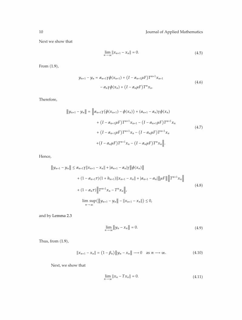
10 Journal of Applied Mathematics
Next we show that
limn→∞
‖xn+1 − xn‖ = 0. (4.5)
From (1.9),
yn+1 − yn = αn+1γφ(xn+1) +(I − αn+1μF
)Tn+1xn+1
− αnγφ(xn) +(I − αnμF
)Tnxn.
(4.6)
Therefore,
∥∥yn+1 − yn
∥∥ =
∥∥∥αn+1γ
(φ(xn+1) − φ(xn)
)+ (αn+1 − αn)γφ(xn)
+(I − αn+1μF
)Tn+1xn+1 −
(I − αn+1μF
)Tn+1xn
+(I − αn+1μF
)Tn+1xn −
(I − αnμF
)Tn+1xn
+(I − αnμF
)Tn+1xn −
(I − αnμF
)Tnxn
∥∥∥.
(4.7)
Hence,
∥∥yn+1 − yn
∥∥ ≤ αn+1γ‖xn+1 − xn‖ + |αn+1 − αn|γ∥∥φ(xn)
∥∥
+ (1 − αn+1τ)(1 + hn+1)‖xn+1 − xn‖ + |αn+1 − αn|∥∥μF
∥∥∥∥∥Tn+1xn
∥∥∥
+ (1 − αnτ)∥∥∥Tn+1xn − Tnxn
∥∥∥,
lim supn→∞
(∥∥yn+1 − yn
∥∥ − ‖xn+1 − xn‖) ≤ 0,
(4.8)
and by Lemma 2.3
limn→∞
∥∥yn − xn
∥∥ = 0. (4.9)
Thus, from (1.9),
‖xn+1 − xn‖ =(1 − βn
)∥∥yn − xn
∥∥ −→ 0 as n −→ ∞. (4.10)
Next, we show that
limn→∞
‖xn − Txn‖ = 0. (4.11)

Journal of Applied Mathematics 11
Since
‖xn − Tnxn‖ ≤ ‖xn+1 − xn‖ + ‖xn+1 − Tnxn‖
= ‖xn+1 − xn‖ +∥∥βnxn +
(1 − βn
)yn − Tnxn
∥∥
≤ ‖xn+1 − xn‖ + βn‖xn − Tnxn‖ +(1 − βn
)αn
(∥∥γφ(xn)∥∥ +
∥∥μFTnxn
∥∥).
(4.12)
Thus,
‖xn − Tnxn‖ ≤ 11 − βn
‖xn+1 − xn‖ + αn
(∥∥γφ(xn)∥∥ +
∥∥μFTnxn
∥∥). (4.13)
Hence,
limn→∞
‖xn − Tnxn‖ = 0. (4.14)
Since T is Lipschitz with constant L and for any positive number n ≥ 1, we have
‖xn − Txn‖ ≤ ‖xn − Tnxn‖ +∥∥∥Tnxn − Tn+1xn
∥∥∥ +∥∥∥Tn+1xn − Txn
∥∥∥
≤ ‖xn − Tnxn‖ +∥∥∥Tnxn − Tn+1xn
∥∥∥ + L‖Tnxn − xn‖ −→ 0.(4.15)
Therefore,
limn→∞
‖xn − Txn‖ = 0. (4.16)
Next we show that
lim supn→∞
⟨γφ
(p) − μFp, Jq
(xn − p
)⟩ ≤ 0, (4.17)
where p ∈ F∗ is the unique solution of inequality (3.2). Let {xnj} be a subsequence of {xn}such that
lim supn→∞
⟨γφ
(p) − μFp, Jq
(xn − p
)⟩= lim
j→∞
⟨γφ
(p) − μFp, Jq
(xnj − p
)⟩. (4.18)
Since {xn} is bounded, we may also assume that there exists some z ∈ C such that xnj ⇀ z.From (4.11) it follows that
xnj − Txnj −→ 0 as j −→ ∞. (4.19)

12 Journal of Applied Mathematics
By Lemma 2.5, the weak limit z ∈ C of {xnj} is a fixed point of the mapping T , so thisimplies that z ∈ F∗. Hence by Theorem 3.1 and Jq is a weakly sequentially continuous dualitymapping, we have
lim supn→∞
〈γφ(p) − μFp, Jq(xn − p
)〉 = 〈γφ(p) − μFp, Jq(z − p
)〉 ≤ 0. (4.20)
Finally, we show that ‖xn − p‖ → 0. By contradiction, there is a number ε0 such that
lim supn→∞
∥∥xn − p
∥∥ ≥ ε0. (4.21)
Case 1. Fixed ε1(ε1 < ε0), if for some n ≥ N ∈ N such that ‖xn − p‖ ≥ ε0 − ε1, and for theother n ≥ N ∈ N such that ‖xn − p‖ < ε0 − ε1.
Let
Mn =2q〈γφp − μFp, Jq
(yn − p
)〉(ε0 − ε1)q
. (4.22)
From (4.20), we know lim supn→∞Mn ≤ 0. Hence, there is a number N, when n > N, wehave Mn ≤ τ − γ . We extract a number n0 ≥ N satisfying ‖xn0 − p‖ < ε0 − ε1, then we estimate‖xn0+1 − p‖
∥∥yn0 − p∥∥q =
∥∥αn0γφ(xn0) +(I − μαn0F
)Tn0xn0 − p
∥∥q
= 〈(I − μαn0F)Tn0xn0−
(I − μαn0F
)p, Jq
(yn0 − p
)〉+αn0
⟨γφ(xn0)−γφ
(p), Jq
(yn0−p
)⟩
+ αn0〈γφ(p) − μFp, Jq
(yn0 − p
)〉
≤ (1 − αn0τ)(1 + hn0)∥∥xn0 − p
∥∥∥∥yn0 − p∥∥q−1 + αn0γ
∥∥φ(xn0) − φ(p)∥∥∥∥yn0 − p
∥∥q−1
+ αn0
⟨γφ
(p) − μFp, Jq
(yn0 − p
)⟩
<[1− αn0
(τ−γ)+(1− αn0τ)hn0
](ε0− ε1)
∥∥yn0 −p∥∥q−1 + αn0
⟨γφ
(p)−μFp, Jq
(yn0−p
)⟩
=[
1 − αn0
[(τ − γ
) − (1 − αn0τ)hn0
αn0
]](ε0 − ε1)
∥∥yn0 − p∥∥q−1

Journal of Applied Mathematics 13
+ αn0
⟨γφ
(p) − μFp, Jq
(yn0 − p
)⟩
≤[1 − αn0
2(τ − γ
)](ε0 − ε1)
∥∥yn0 − p
∥∥q−1 + αn0〈γφ
(p) − μFp, Jq
(yn0 − p
)〉
≤[1 − αn0
2(τ − γ
)]1q(ε0 − ε1)q +
q − 1q
∥∥yn0 − p
∥∥q
+ αn0
⟨γφ
(p) − μFp, Jq
(yn0 − p
)⟩
≤[1 − αn0
2(τ − γ
)](ε0 − ε1)q + qαn0〈γφ
(p) − μFp, Jq
(yn0 − p
)〉.(4.23)
But
∥∥xn0+1 − p∥∥q ≤ βn0
∥∥xn0 − p∥∥q +
(1 − βn0
)∥∥yn0 − p∥∥q
< βn0(ε0 − ε1)q +(1 − βn0
)∥∥yn0 − p∥∥q
.(4.24)
Therefore,
∥∥xn0+1 − p∥∥q
< βn0(ε0 − ε1)q +(1 − βn0
)[1 − αn0
2(τ − γ
)](ε0 − ε1)q
+ qαn0
(1 − βn0
)⟨γφ
(p) − μFp, Jq
(yn0 − p
)⟩
=[
1 − 12αn0
(1 − βn0
)(τ − γ
)](ε0 − ε1)q + qαn0
(1 − βn0
)⟨γφ
(p) − μFp, Jq
(yn0 − p
)⟩
=[
1 − 12αn0
(1 − βn0
)((τ − γ
) −Mn
)](ε0 − ε1)q
< (ε0 − ε1)q.(4.25)
Hence, we have
∥∥xn0+1 − p∥∥ < ε0 − ε1. (4.26)
In the same way, we can get
∥∥xn − p∥∥ < ε0 − ε1, ∀n ≥ n0. (4.27)
It contradicts the lim supn→∞‖xn − p‖ ≥ ε0.Case 2. Fixed ε1(ε1 < ε0), if ‖xn − p‖ ≥ ε0 − ε1, for all n ≥ N ∈ N, from Lemma 2.2, there
is a number r(0 < r < 1) such that
∥∥φ(xn) − φ(p)∥∥ ≤ r
∥∥xn − p∥∥, n ≥ N. (4.28)

14 Journal of Applied Mathematics
It follows (1.9) that
∥∥yn − p
∥∥q =
∥∥αnγφ(xn) + (I − μαnF)Tnxn − p
∥∥q
= 〈(I − μαnF)Tnxn −
(I − μαnF
)p, Jq
(yn − p
)〉 + αn〈γφ(xn) − γφ(p), Jq
(yn − p
)〉+ αn
⟨γφ
(p) − μFp, Jq
(yn − p
)⟩
≤ (1 − αnτ)(1 + hn)∥∥xn − p
∥∥∥∥yn − p
∥∥q−1 + αnγ
∥∥φ(xn) − φ
(p)∥∥
∥∥yn − p
∥∥q−1
+ αn
⟨γφ
(p) − μFp, Jq
(yn − p
)⟩
<[1 − αn
(τ−γr) + (1−αnτ)hn
]∥∥xn − p∥∥∥∥yn− p
∥∥q−1+αn〈γφ
(p) − μFp, Jq
(yn − p
)〉
=[
1 − αn
[(τ − γr
) − (1 − αnτ)hn
αn
]]∥∥xn − p∥∥∥∥yn − p
∥∥q−1
+ αn
⟨γφ
(p) − μFp, Jq
(yn − p
)⟩
≤[1 − αn
2(τ − γr
)]∥∥xn − p∥∥∥∥yn − p
∥∥q−1 + αn〈γφ(p) − μFp, Jq
(yn − p
)〉
≤[1 − αn
2(τ − γr
)]1q
∥∥xn − p∥∥q +
q − 1q
∥∥yn − p∥∥q
+ αn
⟨γφ
(p) − μFp, Jq
(yn − p
)⟩
≤[1 − αn
2(τ − γr
)]∥∥xn − p∥∥q + qαn
⟨γφ
(p) − μFp, Jq
(yn − p
)⟩.
(4.29)
Therefore,
∥∥xn+1 − p∥∥q ≤ βn
∥∥xn − p∥∥q +
(1 − βn
)∥∥yn − p∥∥q
< βn∥∥xn − p
∥∥q +(1 − βn
)[1 − αn
2(τ − γr
)]∥∥xn − p∥∥q
+(1 − βn
)αnq〈γφ
(p) − μFp, Jq
(yn − p
)〉
=[
1 − 12αn
(1 − βn
)(τ − γr
)]∥∥xn − p
∥∥q +(1 − βn
)αnq
⟨γφ
(p) − μFp, Jq
(yn − p
)⟩.
(4.30)
By Lemma 2.4, we have that ‖xn − p‖ → 0 as n → ∞. It contradicts the ‖xn − p‖ ≥ ε0 − ε1.This completes the proof.
The following corollary follows from Theorem 4.1.
Corollary 4.2. Let E be a q-uniformly smooth and strictly convex Banach space, and let C be anonempty closed convex subset of E such that C ± C ⊂ C and have a weakly sequentially continuous
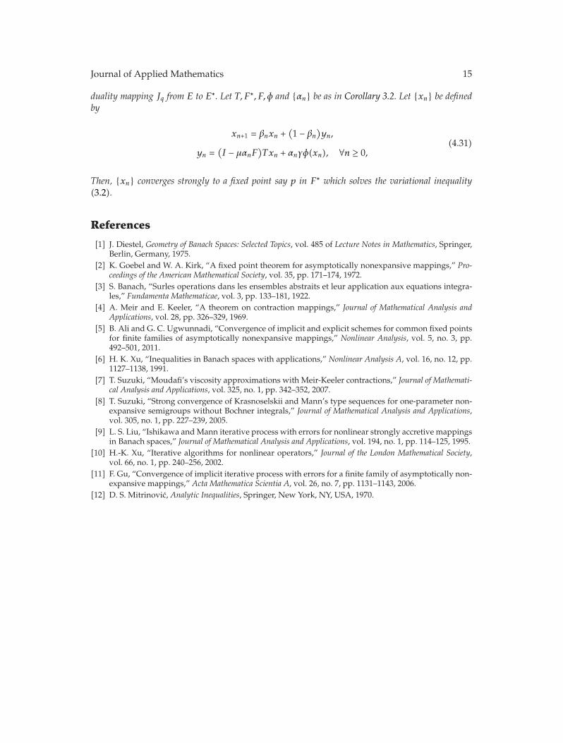
Journal of Applied Mathematics 15
duality mapping Jq from E to E∗. Let T, F∗, F, φ and {αn} be as in Corollary 3.2. Let {xn} be definedby
xn+1 = βnxn +(1 − βn
)yn,
yn =(I − μαnF
)Txn + αnγφ(xn), ∀n ≥ 0,
(4.31)
Then, {xn} converges strongly to a fixed point say p in F∗ which solves the variational inequality(3.2).
References
[1] J. Diestel, Geometry of Banach Spaces: Selected Topics, vol. 485 of Lecture Notes in Mathematics, Springer,Berlin, Germany, 1975.
[2] K. Goebel and W. A. Kirk, “A fixed point theorem for asymptotically nonexpansive mappings,” Pro-ceedings of the American Mathematical Society, vol. 35, pp. 171–174, 1972.
[3] S. Banach, “Surles operations dans les ensembles abstraits et leur application aux equations integra-les,” Fundamenta Mathematicae, vol. 3, pp. 133–181, 1922.
[4] A. Meir and E. Keeler, “A theorem on contraction mappings,” Journal of Mathematical Analysis andApplications, vol. 28, pp. 326–329, 1969.
[5] B. Ali and G. C. Ugwunnadi, “Convergence of implicit and explicit schemes for common fixed pointsfor finite families of asymptotically nonexpansive mappings,” Nonlinear Analysis, vol. 5, no. 3, pp.492–501, 2011.
[6] H. K. Xu, “Inequalities in Banach spaces with applications,” Nonlinear Analysis A, vol. 16, no. 12, pp.1127–1138, 1991.
[7] T. Suzuki, “Moudafi’s viscosity approximations with Meir-Keeler contractions,” Journal of Mathemati-cal Analysis and Applications, vol. 325, no. 1, pp. 342–352, 2007.
[8] T. Suzuki, “Strong convergence of Krasnoselskii and Mann’s type sequences for one-parameter non-expansive semigroups without Bochner integrals,” Journal of Mathematical Analysis and Applications,vol. 305, no. 1, pp. 227–239, 2005.
[9] L. S. Liu, “Ishikawa and Mann iterative process with errors for nonlinear strongly accretive mappingsin Banach spaces,” Journal of Mathematical Analysis and Applications, vol. 194, no. 1, pp. 114–125, 1995.
[10] H.-K. Xu, “Iterative algorithms for nonlinear operators,” Journal of the London Mathematical Society,vol. 66, no. 1, pp. 240–256, 2002.
[11] F. Gu, “Convergence of implicit iterative process with errors for a finite family of asymptotically non-expansive mappings,” Acta Mathematica Scientia A, vol. 26, no. 7, pp. 1131–1143, 2006.
[12] D. S. Mitrinovic, Analytic Inequalities, Springer, New York, NY, USA, 1970.

Hindawi Publishing CorporationJournal of Applied MathematicsVolume 2012, Article ID 516897, 19 pagesdoi:10.1155/2012/516897
Research ArticleStrong Convergence of a Hybrid Iteration Schemefor Equilibrium Problems, Variational InequalityProblems and Common Fixed Point Problems, ofQuasi-φ-Asymptotically Nonexpansive Mappingsin Banach Spaces
Jing Zhao1, 2
1 College of Science, Civil Aviation University of China, Tianjin 300300, China2 Tianjin Key Laboratory for Advanced Signal Processing, Civil Aviation University of China,Tianjin 300300, China
Correspondence should be addressed to Jing Zhao, [email protected]
Received 3 April 2012; Accepted 5 June 2012
Academic Editor: Hong-Kun Xu
Copyright q 2012 Jing Zhao. This is an open access article distributed under the CreativeCommons Attribution License, which permits unrestricted use, distribution, and reproduction inany medium, provided the original work is properly cited.
We introduce an iterative algorithm for finding a common element of the set of commonfixed points of a finite family of closed quasi-φ-asymptotically nonexpansive mappings, the setof solutions of an equilibrium problem, and the set of solutions of the variational inequalityproblem for a γ-inverse strongly monotone mapping in Banach spaces. Then we study thestrong convergence of the algorithm. Our results improve and extend the corresponding resultsannounced by many others.
1. Introduction and Preliminary
Let E be a Banach space with the dual E∗. A mapping A : D(A) ⊂ E → E∗ is said to bemonotone if, for each x, y ∈ D(A), the following inequality holds:
⟨Ax −Ay, x − y
⟩ ≥ 0. (1.1)
A is said to be γ-inverse strongly monotone if there exists a positive real number γ such that
⟨x − y,Ax −Ay
⟩ ≥ γ∥∥Ax −Ay
∥∥2, ∀x, y ∈ D(A). (1.2)

2 Journal of Applied Mathematics
If A is γ-inverse strongly monotone, then it is Lipschitz continuous with constant 1/γ , that is,‖Ax −Ay‖ ≤ (1/γ)‖x − y‖, for all x, y ∈ D(A), and hence uniformly continuous.
Let C be a nonempty closed convex subset of E and f : C×C → R a bifunction, whereR is the set of real numbers. The equilibrium problem for f is to find x ∈ C such that
f(x, y
) ≥ 0 (1.3)
for all y ∈ C. The set of solutions of (1.3) is denoted by EP(f). Given a mapping T : C → E∗,let f(x, y) = 〈Tx, y − x〉 for all x, y ∈ C. Then x ∈ EP(f) if and only if 〈Tx, y − x〉 ≥ 0 forall y ∈ C; that is, x is a solution of the variational inequality. Numerous problems in physics,optimization, engineering, and economics reduce to find a solution of (1.3). Some methodshave been proposed to solve the equilibrium problem; see, for example, Blum and Oettli[1] and Moudafi [2]. For solving the equilibrium problem, let us assume that f satisfies thefollowing conditions:
(A1) f(x, x) = 0 for all x ∈ C;
(A2) f is monotone, that is, f(x, y) + f(y, x) ≤ 0 for all x, y ∈ C;
(A3) for each x, y, z ∈ C, limt→ 0f(tz + (1 − t)x, y) ≤ f(x, y);
(A4) for each x ∈ C, the function y �→ f(x, y) is convex and lower semicontinuous.
Let E be a Banach space with the dual E∗. We denote by J the normalized dualitymapping from E to 2E
∗defined by
J(x) ={x∗ ∈ E∗ : 〈x, x∗〉 = ‖x‖2 = ‖x∗‖2
}, (1.4)
where 〈·, ·〉 denotes the generalized duality pairing. Let dimE ≥ 2, and the modulus ofsmoothness of E is the function ρE : [0,∞) → [0,∞) defined by
ρE(τ) = sup
{∥∥x + y∥∥ +
∥∥x − y∥∥
2− 1 : ‖x‖ = 1;
∥∥y∥∥ = τ
}
. (1.5)
The space E is said to be smooth if ρE(τ) > 0, for all τ > 0 and E is called uniformly smooth ifand only if limt→ 0+(ρE(t)/t) = 0. A Banach space E is said to be strictly convex if ‖x+y‖/2 < 1for x, y ∈ E with ‖x‖ = ‖y‖ = 1 and x /=y. The modulus of convexity of E is the functionδE : (0, 2] → [0, 1] defined by
δE(ε) = inf{
1 −∥∥∥∥x + y
2
∥∥∥∥ : ‖x‖ =∥∥y
∥∥ = 1; ε =∥∥x − y
∥∥}. (1.6)
E is called uniformly convex if and only if δE(ε) > 0 for every ε ∈ (0, 2]. Let p > 1, then Eis said to be p-uniformly convex if there exists a constant c > 0 such that δE(ε) ≥ cεp for allε ∈ (0, 2]. Observe that every p-uniformly convex space is uniformly convex. We know that ifE is uniformly smooth, strictly convex, and reflexive, then the normalized duality mapping Jis single-valued, one-to-one, onto and uniformly norm-to-norm continuous on each boundedsubset of E. Moreover, if E is a reflexive and strictly convex Banach space with a strictly

Journal of Applied Mathematics 3
convex dual, then J−1 is single-valued, one-to-one, surjective, and it is the duality mappingfrom E∗ into E and thus JJ−1 = IE∗ and J−1J = IE (see, [3]). It is also well known that E isuniformly smooth if and only if E∗ is uniformly convex.
Let C be a nonempty closed convex subset of a Banach space E and T : C → C amapping. A point x ∈ C is said to be a fixed point of T provided Tx = x. A point x ∈ C is saidto be an asymptotic fixed point of T provided C contains a sequence {xn} which convergesweakly to x such that limn→∞‖xn − Txn‖ = 0. In this paper, we use F(T) and F(T) to denotethe fixed point set and the asymptotic fixed point set of T and use → to denote the strongconvergence and weak convergence, respectively. Recall that a mapping T : C → C is callednonexpansive if
∥∥Tx − Ty
∥∥ ≤ ∥
∥x − y∥∥, ∀x, y ∈ C. (1.7)
A mapping T : C → C is called asymptotically nonexpansive if there exists a sequence {kn}of real numbers with kn → 1 as n → ∞ such that
∥∥Tnx − Tny∥∥ ≤ kn
∥∥x − y∥∥, ∀x, y ∈ C, ∀n ≥ 1. (1.8)
The class of asymptotically nonexpansive mappings was introduced by Goebel andKirk [4] in 1972. They proved that if C is a nonempty bounded closed convex subset of auniformly convex Banach space E, then every asymptotically nonexpansive self-mapping Tof C has a fixed point. Further, the set F(T) is closed and convex. Since 1972, a host of authorshave studied the weak and strong convergence problems of the iterative algorithms for sucha class of mappings (see, e.g., [4–6] and the references therein).
It is well known that if C is a nonempty closed convex subset of a Hilbert space H andPC : H → C is the metric projection of H onto C, then PC is nonexpansive. This fact actuallycharacterizes Hilbert spaces and, consequently, it is not available in more general Banachspaces. In this connection, Alber [7] recently introduced a generalized projection operatorΠC in a Banach space E which is an analogue of the metric projection in Hilbert spaces.
Next, we assume that E is a smooth Banach space. Consider the functional defined by
φ(x, y
)= ‖x‖2 − 2
⟨x, Jy
⟩+∥∥y
∥∥2, ∀x, y ∈ E. (1.9)
Following Alber [7], the generalized projection ΠC : E → C is a mapping that assigns to anarbitrary point x ∈ E the minimum point of the functional φ(y, x), that is, ΠCx = x, where xis the solution to the following minimization problem:
φ(x, x) = infy∈C
φ(y, x
). (1.10)
It follows from the definition of the function φ that
(∥∥y∥∥ − ‖x‖)2 ≤ φ
(y, x
) ≤ (∥∥y∥∥ + ‖x‖)2
, ∀x, y ∈ E. (1.11)
If E is a Hilbert space, then φ(y, x) = ‖y − x‖2 and ΠC = PC is the metric projection of H ontoC.

4 Journal of Applied Mathematics
Remark 1.1 (see [8, 9]). If E is a reflexive, strictly convex, and smooth Banach space, then forx, y ∈ E, φ(x, y) = 0 if and only if x = y.
Let C be a nonempty, closed, and convex subset of a smooth Banach E and Ta mapping from C into itself. The mapping T is said to be relatively nonexpansive ifF(T) = F(T)/= ∅, φ(p, Tx) ≤ φ(p, x), for allx ∈ C, p ∈ F(T). The mapping T is said tobe φ-nonexpansive if φ(Tx, Ty) ≤ φ(x, y), for allx, y ∈ C. The mapping T is said to bequasi-φ-nonexpansive if F(T)/= ∅, φ(p, Tx) ≤ φ(p, x), for allx ∈ C, p ∈ F(T). The mappingT is said to be relatively asymptotically nonexpansive if there exists some real sequence{kn} with kn ≥ 1 and kn → 1 as n → ∞ such that F(T) = F(T)/= ∅, φ(p, Tnx) ≤knφ(p, x), for allx ∈ C, p ∈ F(T). The mapping T is said to be φ-asymptotically nonexpansiveif there exists some real sequence {kn} with kn ≥ 1 and kn → 1 as n → ∞ such thatφ(Tnx, Tny) ≤ knφ(x, y), for allx, y ∈ C. The mapping T is said to be quasi-φ-asymptoticallynonexpansive if there exists some real sequence {kn} with kn ≥ 1 and kn → 1 as n → ∞such that F(T)/= ∅, φ(p, Tnx) ≤ knφ(p, x), for allx ∈ C, p ∈ F(T). The mapping T is said to beasymptotically regular on C if, for any bounded subset K of C, lim supn→∞{‖Tn+1x − Tnx‖ :x ∈ K} = 0. The mapping T is said to be closed on C if, for any sequence {xn} such thatlimn→∞xn = x0 and limn→∞Txn = y0, Tx0 = y0.
We remark that a φ-asymptotically nonexpansive mapping with a nonempty fixedpoint set F(T) is a quasi-φ-asymptotically nonexpansive mapping, but the converse maybe not true. The class of quasi-φ-nonexpansive mappings and quasi-φ-asymptoticallynonexpansive mappings is more general than the class of relatively nonexpansive mappingsand relatively asymptotically nonexpansive mappings, respectively.
Recently, many authors studied the problem of finding a common element of the set offixed points of nonexpansive or relatively nonexpansive mappings, the set of solutions of anequilibrium problem, and the set of solutions of variational inequalities in the frame work ofHilbert spaces and Banach spaces, respectively; see, for instance, [10–21] and the referencestherein.
In 2009, Takahashi and Zembayashi [22] introduced the following iterative process:
x0 = x ∈ C,
yn = J−1(αnJxn + (1 − αn)JSxn),
un ∈ C, f(un, y
)+
1rn
⟨y − un, Jun − Jyn
⟩ ≥ 0, ∀y ∈ C,
Hn ={z ∈ C : φ(z, un) ≤ φ(z, xn)
},
Wn = {z ∈ C : 〈xn − z, Jx − Jxn〉 ≥ 0},xn+1 = ΠHn∩Wnx, ∀n ≥ 1,
(1.12)
where f : C × C → R is a bifunction satisfying (A1)–(A4), J is the normalized dualitymapping on E and S : C → C is a relatively nonexpansive mapping. They proved thesequence {xn} defined by (1.12) converges strongly to a common point of the set of solutionsof the equilibrium problem (1.3) and the set of fixed points of S provided the controlsequences {αn} and {rn} satisfy appropriate conditions in Banach spaces.

Journal of Applied Mathematics 5
Qin et al. [8] introduced the following iterative scheme on the equilibrium problem(1.3) and a family of quasi-φ-nonexpansive mapping:
x0 ∈ E, C1 = C, x1 = ΠC1x0,
yn = J−1(αn,0Jxn + ΣN
i=1αn,iJTixn
),
un ∈ C, f(un, y
)+
1rn
⟨y − un, Jun − Jyn
⟩ ≥ 0, ∀y ∈ C,
Cn+1 ={z ∈ Cn : φ(z, un) ≤ φ(z, xn)
},
xn+1 = ΠCn+1x0, ∀n ≥ 1.
(1.13)
Strong convergence theorems of common elements are established in a uniformly smoothand strictly convex Banach space which also enjoys the Kadec-Klee property.
Very recently, for finding a common element of ∩ri=1F(Ti) ∩ EP(f, B) ∩ VI(A,C) Zegeye
[23] proposed the following iterative algorithm:
x0 ∈ C0 = C,
zn = ΠCJ−1(Jxn − λnAxn),
yn = J−1(α0Jxn + Σri=1αiJTizn
),
un ∈ C, f(un, y
)+
1rn
⟨y − un, Jun − Jyn
⟩ ≥ 0, ∀y ∈ C,
Cn+1 ={z ∈ Cn : φ(z, un) ≤ φ(z, xn)
},
xn+1 = ΠCn+1x0, ∀n ≥ 1,
(1.14)
where Ti : C → C is closed quasi-φ-nonexpansive mapping (i = 1, . . . , r), f : C × C → R
is a bifunction satisfying (A1)–(A4) and A is a γ-inverse strongly monotone mapping of Cinto E∗. Strong convergence theorems for iterative scheme (1.14) are obtained under someconditions on parameters in 2-uniformly convex and uniformly smooth real Banach space E.
In this paper, inspired and motivated by the works mentioned above, we introducean iterative process for finding a common element of the set of common fixed points of afinite family of closed quasi-φ-asymptotically nonexpansive mappings, the solution set ofequilibrium problem, and the solution set of the variational inequality problem for a γ-inversestrongly monotone mapping in Banach spaces. The results presented in this paper improveand generalize the corresponding results announced by many others.
In order to the main results of this paper, we need the following lemmas.
Lemma 1.2 (see [24]). Let E be a 2-uniformly convex and smooth Banach space. Then, for all x, y ∈E, one has
∥∥x − y∥∥ ≤ 2
c2
∥∥Jx − Jy∥∥, (1.15)

6 Journal of Applied Mathematics
where J is the normalized duality mapping ofE and 1/c(0 < c ≤ 1) is the 2-uniformly convex constantof E.
Lemma 1.3 (see [7, 25]). Let C be a nonempty closed convex subset of a smooth, strictly convex andreflexive Banach space E. Then
φ(x,ΠCy
)+ φ
(ΠCy, y
) ≤ φ(x, y
), ∀x ∈ C, y ∈ E. (1.16)
Lemma 1.4 (see [25]). Let E be a smooth and uniformly convex Banach space and let {xn} and{yn} be sequences in E such that either {xn} or {yn} is bounded. If limn→∞φ(xn, yn) = 0, thenlimn→∞‖xn − yn‖ = 0.
Lemma 1.5 (see [7]). Let C be a nonempty closed convex subset of a smooth Banach space E, letx ∈ E and let z ∈ C. Then
z = ΠCx ⇐⇒ ⟨y − z, Jx − Jz
⟩ ≤ 0, ∀y ∈ C. (1.17)
We denote by NC(v) the normal cone for C ⊂ E at a point v ∈ C, that is, NC(v) = {x∗ ∈E∗ : 〈v − y, x∗〉 ≥ 0, for ally ∈ C}. We shall use the following lemma.
Lemma 1.6 (see [26]). Let C be a nonempty closed convex subset of a Banach space E and let A be amonotone and hemicontinuous operator of C into E∗ with C = D(A). Let S ⊂ E × E∗ be an operatordefined as follows:
Sv =
{Av +NC(v), v ∈ C,
∅, v /∈ C.(1.18)
Then S is maximal monotone and S−1(0) = VI(C,A).
We make use of the function V : E × E∗ → R defined by
V (x, x∗) = ‖x‖2 − 2〈x, x∗〉 + ‖x∗‖2, (1.19)
for all x ∈ E and x∗ ∈ E∗ (see [7]). That is, V (x, x∗) = φ(x, J−1x∗) for all x ∈ E and x∗ ∈ E∗.
Lemma 1.7 (see [7]). Let E be a reflexive, strictly convex, and smooth Banach space with E∗ as itsdual. Then,
V (x, x∗) + 2⟨J−1x∗ − x, y∗
⟩≤ V
(x, x∗ + y∗) (1.20)
for all x ∈ E and x∗, y∗ ∈ E∗.

Journal of Applied Mathematics 7
Lemma 1.8 (see [1]). Let C be a closed convex subset of a smooth, strictly convex, and reflexiveBanach space E, let f be a bifunction from C ×C to R satisfying (A1)–(A4), and let r > 0 and x ∈ E.Then, there exists z ∈ C such that
f(z, y
)+
1r
⟨y − z, Jz − Jx
⟩ ≥ 0, ∀y ∈ C. (1.21)
Lemma 1.9 (see [22]). Let C be a closed convex subset of a uniformly smooth, strictly convex, andreflexive Banach space E. Let f be a bifunction from C × C to R satisfying (A1)–(A4). For r > 0 andx ∈ E, define a mapping Tr : E → C as follows:
Tr(x) ={z ∈ C : f
(z, y
)+
1r
⟨y − z, Jz − Jx
⟩ ≥ 0, ∀y ∈ C
}(1.22)
for all x ∈ E. Then, the following hold:
(1) Tr is single-valued;
(2) Tr is firmly nonexpansive, that is, for any x, y ∈ E,
⟨Trx − Try, JTrx − JTry
⟩ ≤ ⟨Trx − Try, Jx − Jy
⟩; (1.23)
(3) F(Tr) = EP(f);
(4) EP(f) is closed and convex;
(5) φ(q, Trx) + φ(Trx, x) ≤ φ(q, x), for all q ∈ F(Tr).
Lemma 1.10 (see [8, 23]). Let E be a uniformly convex Banach space, s > 0 a positive numberand Bs(0) a closed ball of E. Then there exists a strictly increasing, continuous, and convex functiong : [0,∞) → [0,∞) with g(0) = 0 such that
∥∥∥∥∥
N∑
i=0(αixi)
∥∥∥∥∥
2
≤N∑
i=0
αi‖xi‖2 − αkαlg(‖xk − xl‖) (1.24)
for any k, l ∈ {0, 1, . . . ,N}, for all x0, x1, . . . , xN ∈ Bs(0) = {x ∈ E : ‖x‖ ≤ s} and α0, α1, . . . , αn ∈[0, 1] such that
∑Ni=0 αi = 1.
Lemma 1.11 (see [27]). Let E be a uniformly convex and uniformly smooth Banach space, Ca nonempty, closed, and convex subset of E, and T a closed quasi-φ-asymptotically nonexpansivemapping from C into itself. Then F(T) is a closed convex subset of C.
2. Main Results
Theorem 2.1. Let C be a nonempty, closed, and convex subset of a 2-uniformly convex and uniformlysmooth real Banach space E and Ti : C → C a closed quasi-φ-asymptotically nonexpansive mappingwith sequence {kn,i} ⊂ [1,∞) such that limn→∞kn,i = 1 for each 1 ≤ i ≤ N. Let f be a bifunctionfrom C × C to R satisfying (A1)–(A4). Let A be a γ-inverse strongly monotone mapping of C into E∗

8 Journal of Applied Mathematics
with constant γ > 0 such that F = (⋂N
i=1 F(Ti))⋂
EP(f)⋂
VI(C,A)/= ∅ and F is bounded. Assumethat Ti is asymptotically regular on C for each 1 ≤ i ≤ N and ‖Ax‖ ≤ ‖Ax −Ap‖ for all x ∈ C andp ∈ F. Define a sequence {xn} in C in the following manner:
x0 ∈ C0 = C chosen arbitrarily,
zn = ΠCJ−1(Jxn − λnAxn),
yn = J−1(αn,0Jxn + αn,1JTn1 zn + · · · + αn,NJTn
Nzn),
un ∈ C, f(un, y
)+
1rn
⟨y − un, Jun − Jyn
⟩ ≥ 0, ∀y ∈ C,
Cn+1 =
{
z ∈ Cn : φ(z, un) ≤ φ(z, xn) +N∑
i=1
αn,i(kn,i − 1)Ln
}
,
xn+1 = ΠCn+1x0
(2.1)
for every n ≥ 0, where {rn} is a real sequence in [a,∞) for some a > 0, J is the normalized dualitymapping on E and Ln = sup{φ(p, xn) : p ∈ F} < ∞. Assume that {αn,0}, {αn,1}, . . ., {αn,N} are realsequences in (0, 1) such that
∑Ni=0 αn,i = 1 and lim infn→∞αn,0αn,i > 0, for all i ∈ {1, 2, . . . ,N}. Let
{λn} be a sequence in [s, t] for some 0 < s < t < c2γ/2, where 1/c is the 2-uniformly convex constantof E. Then the sequence {xn} converges strongly toΠFx0.
Proof. We break the proof into nine steps.
Step 1. ΠFx0 is well defined for x0 ∈ C.By Lemma 1.11 we know that F(Ti) is a closed convex subset of C for every 1 ≤ i ≤
N. Hence F = (⋂N
i=1 F(Ti))⋂
EP(f)⋂
VI(C,A)/= ∅ is a nonempty closed convex subset of C.Consequently, ΠFx0 is well defined for x0 ∈ C.
Step 2. Cn is closed and convex for each n ≥ 0.It is obvious that C0 = C is closed and convex. Suppose that Cn is closed and convex
for some integer n. Since the defining inequality in Cn+1 is equivalent to the inequality:
2〈z, Jxn − Jun〉 ≤ ‖xn‖2 − ‖un‖2 +N∑
i=1
αn,i(kn,i − 1)Ln, (2.2)
we have that Cn+1 is closed and convex. So Cn is closed and convex for each n ≥ 0. This inturn shows that ΠCn+1x0 is well defined.
Step 3. F ⊂ Cn for all n ≥ 0.

Journal of Applied Mathematics 9
We do this by induction. For n = 0, we have F ⊂ C = C0. Suppose that F ⊂ Cn for somen ≥ 0. Let p ∈ F ⊂ C. Putting un = Trnyn for all n ≥ 0, we have that Trn is quasi-φ-nonexpansivefrom Lemma 1.9. Since Ti is quasi-φ-asymptotically nonexpansive, we have
φ(p, un
)= φ
(p, Trnyn
) ≤ φ(p, yn
)
= φ
(
p, J−1
(
αn,0Jxn +N∑
i=1
αn,iJTni zn
))
=∥∥p
∥∥2 − 2
⟨
p, αn,0Jxn +N∑
i=1
αn,iJTni zn
⟩
+
∥∥∥∥∥αn,0Jxn +
N∑
i=1
αn,iJTni zn
∥∥∥∥∥
2
≤ ∥∥p
∥∥2 − 2αn,0
⟨p, Jxn
⟩ − 2N∑
i=1
αn,i
⟨p, JTn
i zn⟩+ αn,0‖xn‖2 +
N∑
i=1
αn,i
∥∥Tn
i zn∥∥2
= αn,0φ(p, xn
)+
N∑
i=1
αn,iφ(p, Tn
i zn)
≤ αn,0φ(p, xn
)+
N∑
i=1
αn,ikn,iφ(p, zn
).
(2.3)
Moreover, by Lemmas 1.3 and 1.7, we get that
φ(p, zn
)
= φ(p,ΠCJ
−1(Jxn − λnAxn))
≤ φ(p, J−1(Jxn − λnAxn)
)
= V(p, Jxn − λnAxn
)
≤ V(p, (Jxn − λnAxn) + λnAxn
) − 2⟨J−1(Jxn − λnAxn) − p, λnAxn
⟩
= V(p, Jxn
) − 2λn⟨J−1(Jxn − λnAxn) − p,Axn
⟩
= φ(p, xn
) − 2λn⟨xn − p,Axn
⟩ − 2λn⟨J−1(Jxn − λnAxn) − xn,Axn
⟩
≤ φ(p, xn
) − 2λn⟨xn − p,Axn −Ap
⟩ − 2λn⟨xn − p,Ap
⟩
+ 2⟨J−1(Jxn − λnAxn) − xn,−λnAxn
⟩.
(2.4)
Thus, since p ∈ VI(C,A) and A is γ-inverse strongly monotone, we have from (2.4) that
φ(p, zn
) ≤ φ(p, xn
) − 2λnγ∥∥Axn −Ap
∥∥2 + 2⟨J−1(Jxn − λnAxn) − xn,−λnAxn
⟩. (2.5)

10 Journal of Applied Mathematics
Therefore, from (2.5), Lemma 1.2 and the fact that λn < c2γ/2 and ‖Ax‖ ≤ ‖Ax −Ap‖ for allx ∈ C and p ∈ F, we have
φ(p, zn
) ≤ φ(p, xn
) − 2λnγ∥∥Axn −Ap
∥∥2 +
4c2λ2n
∥∥Axn −Ap
∥∥2
= φ(p, xn
)+ 2λn
(2c2λn − γ
)∥∥Axn −Ap
∥∥2
≤ φ(p, xn
).
(2.6)
Substituting (2.6) into (2.3), we get
φ(p, un
) ≤ φ(p, xn
)+
N∑
i=1
αn,i(kn,i − 1)Ln, (2.7)
that is, p ∈ Cn+1. By induction, F ⊂ Cn and the iteration algorithm generated by (2.1) is welldefined.
Step 4. limn→∞φ(xn, x0) exists and {xn} is bounded.Noticing that xn = ΠCnx0 and Lemma 1.3, we have
φ(xn, x0) = φ(ΠCnx0, x0) ≤ φ(p, x0
) − φ(p, xn
) ≤ φ(p, x0
)(2.8)
for all p ∈ F and n ≥ 0. This shows that the sequence {φ(xn, x0)} is bounded. From xn = ΠCnx0
and xn+1 = ΠCn+1x0 ∈ Cn+1 ⊂ Cn, we obtain that
φ(xn, x0) ≤ φ(xn+1, x0), ∀n ≥ 0, (2.9)
which implies that {φ(xn, x0)} is nondecreasing. Therefore, the limit of {φ(xn, x0)} exists and{xn} is bounded.
Step 5. We have xn → x∗ ∈ C.By Lemma 1.3, we have, for any positive integer m ≥ n, that
φ(xm, xn) = φ(xm,ΠCnx0) ≤ φ(xm, x0) − φ(ΠCnx0, x0) = φ(xm, x0) − φ(xn, x0). (2.10)
In view of Step 4 we deduce that φ(xm, xn) → 0 as m,n → ∞. It follows from Lemma 1.4that ‖xm − xn‖ → 0 as m,n → ∞. Hence {xn} is a Cauchy sequence of C. Since E is a Banachspace and C is closed subset of E, there exists a point x∗ ∈ C such that xn → x∗ (n → ∞).
Step 6. We have x∗ ∈ ⋂Ni=1 F(Ti).
By taking m = n + 1 in (2.10), we have
limn→∞
φ(xn+1, xn) = 0. (2.11)

Journal of Applied Mathematics 11
From Lemma 1.4, it follows that
limn→∞
‖xn+1 − xn‖ = 0. (2.12)
Noticing that xn+1 ∈ Cn+1, we obtain
φ(xn+1, un) ≤ φ(xn+1, xn) +N∑
i=1
αn,i(kn,i − 1)Ln. (2.13)
From (2.11), limn→∞kn,i = 1 for any 1 ≤ i ≤ N, and Lemma 1.4, we know
limn→∞
‖xn+1 − un‖ = 0. (2.14)
Notice that
‖xn − un‖ ≤ ‖xn − xn+1‖ + ‖xn+1 − un‖ (2.15)
for all n ≥ 0. It follows from (2.12) and (2.14) that
limn→∞
‖xn − un‖ = 0, (2.16)
which implies that un → x∗ as n → ∞. Since J is uniformly norm-to-norm continuous onbounded sets, from (2.16), we have
limn→∞
‖Jxn − Jun‖ = 0. (2.17)
Let s = sup{‖xn‖, ‖Tn1 xn‖, ‖Tn
2 xn‖, . . . , ‖TnNxn‖ : n ∈ N}. Since E is uniformly smooth Banach
space, we know that E∗ is a uniformly convex Banach space. Therefore, from Lemma 1.10 wehave, for any p ∈ F, that
φ(p, un
)= φ
(p, Trnyn
)
≤ φ(p, yn
)
= φ
(
p, J−1
(
αn,0Jxn +N∑
i=1
αn,iJTni zn
))
=∥∥p
∥∥2 − 2αn,0⟨p, Jxn
⟩ − 2N∑
i=1
αn,i
⟨p, JTn
i zn⟩+
∥∥∥∥∥αn,0Jxn +
N∑
i=1
αn,iJTni zn
∥∥∥∥∥
2

12 Journal of Applied Mathematics
≤ ∥∥p
∥∥2 − 2αn,0
⟨p, Jxn
⟩ − 2N∑
i=1
αn,i
⟨p, JTn
i zn⟩+ αn,0‖xn‖2
+N∑
i=1
αn,i
∥∥Tn
i zn∥∥2 − αn,0αn,1g
(∥∥Jxn − JTn1 zn
∥∥)
= αn,0φ(p, xn
)+
N∑
i=1
αn,iφ(p, Tn
i zn) − αn,0αn,1g
(∥∥Jxn − JTn1 zn
∥∥)
≤ αn,0φ(p, xn
)+
N∑
i=1
αn,ikn,iφ(p, zn
) − αn,0αn,1g(∥∥Jxn − JTn
1 zn∥∥).
(2.18)
Therefore, from (2.6) and (2.18), we have
φ(p, un
) ≤ φ(p, xn
)+
N∑
i=1
αn,i(kn,i − 1)φ(p, xn
) − αn,0αn,1g(∥∥Jxn − JTn
1 zn∥∥)
+ 2λn(
2c2λn − γ
)∥∥Axn −Ap∥∥2
N∑
i=1
αn,ikn,i.
(2.19)
It follows from λn < c2γ/2 that
αn,0αn,1g(∥∥Jxn − JTn
1 zn∥∥) ≤ φ
(p, xn
) − φ(p, un
)+
N∑
i=1
αn,i(kn,i − 1)φ(p, xn
). (2.20)
On the other hand, we have
∣∣φ(p, xn
) − φ(p, un
)∣∣
=∣∣∣‖xn‖2 − ‖un‖2 − 2
⟨p, Jxn − Jun
⟩∣∣∣
≤ |‖xn‖ − ‖un‖|(‖xn‖ + ‖un‖) + 2‖Jxn − Jun‖∥∥p
∥∥
≤ ‖xn − un‖(‖xn‖ + ‖un‖) + 2‖Jxn − Jun‖∥∥p
∥∥.
(2.21)
It follows from (2.16) and (2.17) that
limn→∞
(φ(p, xn
) − φ(p, un
))= 0. (2.22)
Since limn→∞kn,i = 1 and lim infn→∞αn,0αn,1 > 0, from (2.20) and (2.22) we have
limn→∞
g(∥∥Jxn − JTn
1 zn∥∥) = 0. (2.23)

Journal of Applied Mathematics 13
Therefore, from the property of g, we obtain
limn→∞
∥∥Jxn − JTn
1 zn∥∥ = 0. (2.24)
Since J−1 is uniformly norm-to-norm continuous on bounded sets, we have
limn→∞
∥∥xn − Tn1 zn
∥∥ = 0, (2.25)
and hence Tn1 zn → x∗ as n → ∞. Since ‖Tn+1
1 zn − x∗‖ ≤ ‖Tn+11 zn − Tn
1 zn‖ + ‖Tn1 zn − x∗‖, it
follows from the asymptotic regularity of T1 that
limn→∞
∥∥∥Tn+11 zn − x∗
∥∥∥ = 0. (2.26)
That is, T1(Tn1 zn) → x∗ as n → ∞. From the closedness of T1, we get T1x
∗ = x∗. Similarly, onecan obtain that Tix∗ = x∗ for i = 2, . . . ,N. So, x∗ ∈ ⋂N
i=1 F(Ti).Moreover, from (2.19) we have that
2λn(γ − 2
c2λn
)∥∥Axn −Ap∥∥2(1 − αn,0)
≤ 2λn(γ − 2
c2λn
)∥∥Axn −Ap∥∥2
N∑
i=1
αn,ikn,i
≤ φ(p, xn
) − φ(p, un
)+
N∑
i=1
αn,i(kn,i − 1)φ(p, xn
),
(2.27)
which implies that
limn→∞
∥∥Axn −Ap∥∥ = 0. (2.28)

14 Journal of Applied Mathematics
Now, Lemmas 1.3 and 1.7 imply that
φ(xn, zn) = φ(xn,ΠCJ
−1(Jxn − λnAxn))
≤ φ(xn, J
−1(Jxn − λnAxn))
= V (xn, Jxn − λnAxn)
≤ V (xn, (Jxn − λnAxn) + λnAxn) − 2⟨J−1(Jxn − λnAxn) − xn, λnAxn
⟩
= φ(xn, xn) + 2⟨J−1(Jxn − λnAxn) − xn,−λnAxn
⟩
= 2⟨J−1(Jxn − λnAxn) − xn,−λnAxn
⟩
≤ 2∥∥∥J−1(Jxn − λnAxn) − J−1Jxn
∥∥∥ · ‖λnAxn‖.
(2.29)
In view of Lemma 1.2 and the fact that ‖Ax‖ ≤ ‖Ax −Ap‖ for all x ∈ C, p ∈ F, we have
φ(xn, zn) ≤ 4c2λ2n
∥∥Axn −Ap∥∥2 ≤ 4
c2t2∥∥Axn −Ap
∥∥2. (2.30)
From (2.28) and Lemma 1.4 we get
limn→∞
‖xn − zn‖ = 0, (2.31)
and hence zn → x∗ as n → ∞.
Step 7. We have x∗ ∈ VI(C,A).Let S ⊂ E × E∗ be an operator as follows:
Sv =
{Av +NC(v), v ∈ C,
∅, v /∈ C.(2.32)
By Lemma 1.6, S is maximal monotone and S−1(0) = VI(C,A). Let (v,w) ∈ G(S). Since w ∈Sv = Av +NC(v), we have w −Av ∈ NC(v). It follows from zn ∈ C that
〈v − zn,w −Av〉 ≥ 0. (2.33)
On the other hand, from zn = ΠCJ−1(Jxn − λnAxn) and Lemma 1.5 we obtain that
〈v − zn, Jzn − (Jxn − λnAxn)〉 ≥ 0, (2.34)

Journal of Applied Mathematics 15
and hence
⟨v − zn,
Jxn − Jznλn
−Axn
⟩≤ 0. (2.35)
Then, from (2.33) and (2.35), we have
〈v − zn,w〉 ≥ 〈v − zn,Av〉
≥ 〈v − zn,Av〉 +⟨v − zn,
Jxn − Jznλn
−Axn
⟩
=⟨v − zn,Av −Axn +
Jxn − Jznλn
⟩
= 〈v − zn,Av −Azn〉 + 〈v − zn,Azn −Axn〉 +⟨v − zn,
Jxn − Jznλn
⟩
≥ − ‖v − zn‖ · ‖Azn −Axn‖ − ‖v − zn‖ · ‖Jxn − Jzn‖s
.
(2.36)
Hence we have 〈v − x∗, w〉 ≥ 0 as n → ∞, since the uniform continuity of J and A implythat the right side of (2.36) goes to 0 as n → ∞. Thus, since S is maximal monotone, we havex∗ ∈ S−1(0) and hence x∗ ∈ VI(C,A).
Step 8. We have x∗ ∈ EP(f) = F(Tr).Let p ∈ F. From un = Trnyn, (2.3), (2.6) and Lemma 1.9 we obtain that
φ(un, yn
)= φ
(Trnyn, yn
)
≤ φ(p, yn
) − φ(p, Trnyn
)
≤ φ(p, xn
)+
N∑
i=1
αn,i(kn,i − 1)φ(p, xn
) − φ(p, un
).
(2.37)
It follows from (2.22) and kn,i → 1 that φ(un, yn) → 0 as n → ∞. Now, by Lemma 1.4 wehave that ‖un − yn‖ → 0 as n → ∞. Consequently, we obtain that ‖Jun − Jyn‖ → 0 andyn → x∗ from un → x∗ as n → ∞. From the assumption rn > a, we get
limn→∞
∥∥Jun − Jyn
∥∥
rn= 0. (2.38)
Noting that un = Trnyn, we obtain
f(un, y
)+
1rn
⟨y − un, Jun − Jyn
⟩ ≥ 0, ∀y ∈ C. (2.39)

16 Journal of Applied Mathematics
From (A2), we have
⟨y − un,
Jun − Jyn
rn
⟩≥ −f(un, y
) ≥ f(y, un
), ∀y ∈ C. (2.40)
Letting n → ∞, we have from un → x∗, (2.38) and (A4) that f(y, x∗) ≤ 0 (for all y ∈ C). Fort with 0 < t ≤ 1 and y ∈ C, let yt = ty + (1 − t)x∗. Since y ∈ C and x∗ ∈ C, we have yt ∈ C andhence f(yt, x
∗) ≤ 0. Now, from (A1) and (A4) we have
0 = f(yt, yt
) ≤ tf(yt, y
)+ (1 − t)f
(yt, x
∗) ≤ tf(yt, y
)(2.41)
and hence f(yt, y) ≥ 0. Letting t → 0, from (A3), we have f(x∗, y) ≥ 0. This implies thatx∗ ∈ EP(f). Therefore, in view of Steps 6, 7, and 8 we have x∗ ∈ F.
Step 9. We have x∗ = ΠFx0.From xn = ΠCnx0, we get
〈xn − z, Jx0 − Jxn〉 ≥ 0, ∀z ∈ Cn. (2.42)
Since F ⊂ Cn for all n ≥ 1, we arrive at
⟨xn − p, Jx0 − Jxn
⟩ ≥ 0, ∀p ∈ F. (2.43)
Letting n → ∞, we have
⟨x∗ − p, Jx0 − Jx∗⟩ ≥ 0, ∀p ∈ F, (2.44)
and hence x∗ = ΠFx0 by Lemma 1.5. This completes the proof.
Strong convergence theorem for approximating a common element of the set ofsolutions of the equilibrium problem and the set of fixed points of a finite family of closedquasi-φ-asymptotically nonexpansive mappings in Banach spaces may not require that E be2-uniformly convex. In fact, we have the following theorem.
Theorem 2.2. Let C be a nonempty, closed, and convex subset of a uniformly convex and uniformlysmooth real Banach space E and Ti : C → C a closed quasi-φ-asymptotically nonexpansive mappingwith sequence {kn,i} ⊂ [1,∞) such that limn→∞kn,i = 1 for each 1 ≤ i ≤ N. Let f be a bifunctionfrom C × C to R satisfying (A1)–(A4) such that F = (
⋂Ni=1 F(Ti))
⋂EP(f)/= ∅ and F is bounded.

Journal of Applied Mathematics 17
Assume that Ti is asymptotically regular on C for each 1 ≤ i ≤ N. Define a sequence {xn} in C in thefollowing manner:
x0 ∈ C0 = C chosen arbitrarily,
yn = J−1(αn,0Jxn + αn,1JTn1 xn + · · · + αn,NJTn
Nxn
),
un ∈ C, f(un, y
)+
1rn
⟨y − un, Jun − Jyn
⟩ ≥ 0, ∀y ∈ C,
Cn+1 =
{
z ∈ Cn : φ(z, un) ≤ φ(z, xn) +N∑
i=1
αn,i(kn,i − 1)Ln
}
,
xn+1 = ΠCn+1x0
(2.45)
for every n ≥ 0, where {rn} is a real sequence in [a,∞) for some a > 0, J is the normalized dualitymapping on E and Ln = sup{φ(p, xn) : p ∈ F} < ∞. Assume that {αn,0}, {αn,1}, . . ., {αn,N} are realsequences in (0, 1) such that
∑Ni=0 αn,i = 1 and lim infn→∞αn,0αn,i > 0, for all i ∈ {1, 2, . . . ,N}. Then
the sequence {xn} converges strongly toΠFx0.
Proof. Put A ≡ 0 in Theorem 2.1. We have zn = xn. Thus, the method of proof of Theorem 2.1gives the required assertion without the requirement that E is 2-uniformly convex.
As some corollaries of Theorems 2.1 and 2.2, we have the following resultsimmediately.
Corollary 2.3. Let C be a nonempty, closed, and convex subset of a Hilbert space H and Ti : C →C a closed quasi-φ-asymptotically nonexpansive mapping with sequence {kn,i} ⊂ [1,∞) such thatlimn→∞kn,i = 1 for each 1 ≤ i ≤ N. Let f be a bifunction from C × C to R satisfying (A1)–(A4).Let A be a γ-inverse strongly monotone mapping of C into H with constant γ > 0 such that F =(⋂N
i=1 F(Ti))⋂
EP(f)⋂
VI (C,A)/= ∅ and F is bounded. Assume that Ti is asymptotically regularon C for each 1 ≤ i ≤ N and ‖Ax‖ ≤ ‖Ax −Ap‖ for all x ∈ C and p ∈ F. Define a sequence {xn} inC in the following manner:
x0 ∈ C0 = C chosen arbitrarily,
zn = PC(xn − λnAxn),
yn = αn,0xn + αn,1Tn1 zn + · · · + αn,NTn
Nzn,
un ∈ C, f(un, y
)+
1rn
⟨y − un, un − yn
⟩ ≥ 0, ∀y ∈ C,
Cn+1 =
{
z ∈ Cn : ‖z − un‖2 ≤ ‖z − xn‖2 +N∑
i=1
αn,i(kn,i − 1)Ln
}
,
xn+1 = PCn+1x0
(2.46)
for every n ≥ 0, where {rn} is a real sequence in [a,∞) for some a > 0 and Ln = sup{‖xn − p‖2 : p ∈F} < ∞. Assume that {αn,0}, {αn,1}, . . ., {αn,N} are real sequences in (0, 1) such that
∑Ni=0 αn,i = 1

18 Journal of Applied Mathematics
and lim infn→∞αn,0αn,i > 0, for all i ∈ {1, 2, . . . ,N}. Let {λn} be a sequence in [s, t] for some0 < s < t < γ/2. Then the sequence {xn} converges strongly to PFx0.
Corollary 2.4. Let C be a nonempty, closed, and convex subset of a Hilbert space H and Ti : C →C a closed quasi-φ-asymptotically nonexpansive mapping with sequence {kn,i} ⊂ [1,∞) such thatlimn→∞kn,i = 1 for each 1 ≤ i ≤ N. Let f be a bifunction from C×C to R satisfying (A1)–(A4) suchthat F = (
⋂Ni=1 F(Ti))
⋂EP(f)/= ∅ and F is bounded. Assume that Ti is asymptotically regular on C
for each 1 ≤ i ≤ N. Define a sequence {xn} in C in the following manner:
x0 ∈ C0 = C chosen arbitrarily,
yn = αn,0xn + αn,1Tn1 xn + · · · + αn,NTn
Nxn,
un ∈ C, f(un, y
)+
1rn
⟨y − un, un − yn
⟩ ≥ 0, ∀y ∈ C,
Cn+1 =
{
z ∈ Cn : ‖z − un‖2 ≤ ‖z − xn‖2 +N∑
i=1
αn,i(kn,i − 1)Ln
}
,
xn+1 = PCn+1x0
(2.47)
for every n ≥ 0, where {rn} is a real sequence in [a,∞) for some a > 0 and Ln = sup{‖xn − p‖2 : p ∈F} < ∞. Assume that {αn,0}, {αn,1}, . . ., {αn,N} are real sequences in (0, 1) such that
∑Ni=0 αn,i = 1
and lim infn→∞αn,0αn,i > 0, for all i ∈ {1, 2, . . . ,N}. Let {λn} be a sequence in [s, t] for some0 < s < t < γ/2. Then the sequence {xn} converges strongly to PFx0.
Remark 2.5. Theorems 2.1 and 2.2 extend the main results of [23] from quasi-φ-nonexpansivemappings to more general quasi-φ-asymptotically nonexpansive mappings.
Acknowledgments
The research was supported by Fundamental Research Funds for the Central Universities(Program no. ZXH2012K001), supported in part by the Foundation of Tianjin Key Lab forAdvanced Signal Processing and it was also supported by the Science Research FoundationProgram in Civil Aviation University of China (2012KYM04).
References
[1] E. Blum and W. Oettli, “From optimization and variational inequalities to equilibrium problems,” TheMathematics Student, vol. 63, no. 1–4, pp. 123–145, 1994.
[2] A. Moudafi, “Second-order differential proximal methods for equilibrium problems,” Journal ofInequalities in Pure and Applied Mathematics, vol. 4, no. 1, article 18, 2003.
[3] W. Takahashi, Nonlinear Functional Analysis, Kindikagaku, Tokyo, Japan, 1988.[4] K. Goebel and W. A. Kirk, “A fixed point theorem for asymptotically nonexpansive mappings,”
Proceedings of the American Mathematical Society, vol. 35, pp. 171–174, 1972.[5] J. Schu, “Iterative construction of fixed points of asymptotically nonexpansive mappings,” Journal of
Mathematical Analysis and Applications, vol. 158, no. 2, pp. 407–413, 1991.[6] H. Y. Zhou, Y. J. Cho, and S. M. Kang, “A new iterative algorithm for approximating common fixed
points for asymptotically nonexpansive mappings,” Fixed Point Theory and Applications, vol. 2007,Article ID 64874, 10 pages, 2007.

Journal of Applied Mathematics 19
[7] Y. I. Alber, “Metric and generalized projection operators in Banach spaces: properties andapplications,” in Theory and Applications of Nonlinear Operators of Accretive and Monotone Type, vol.178, pp. 15–50, Marcel Dekker, New York, NY, USA, 1996.
[8] X. Qin, S. Y. Cho, and S. M. Kang, “Strong convergence of shrinking projection methods for quasi-φ-nonexpansive mappings and equilibrium problems,” Journal of Computational and AppliedMathematics,vol. 234, no. 3, pp. 750–760, 2010.
[9] H. Zhou, G. Gao, and B. Tan, “Convergence theorems of a modified hybrid algorithm for a family ofquasi-φ-asymptotically nonexpansive mappings,” Journal of Applied Mathematics and Computing, vol.32, no. 2, pp. 453–464, 2010.
[10] F. Cianciaruso, G. Marino, L. Muglia, and Y. Yao, “A hybrid projection algorithm for findingsolutions of mixed equilibrium problem and variational inequality problem,” Fixed Point Theory andApplications, vol. 2010, Article ID 383740, 19 pages, 2010.
[11] F. Cianciaruso, G. Marino, L. Muglia, and Y. Yao, “On a two-step algorithm for hierarchical fixedpoint problems and variational inequalities,” Journal of Inequalities and Applications, vol. 2009, ArticleID 208692, 13 pages, 2009.
[12] S. Saewan and P. Kumam, “A modified hybrid projection method for solving generalized mixedequilibrium problems and fixed point problems in Banach spaces,” Computers and Mathematics withApplications, vol. 62, no. 4, pp. 1723–1735, 2011.
[13] S. Saewan and P. Kumam, “Convergence theorems for mixed equilibrium problems, variationalinequality problem and uniformly quasi-φ-asymptotically nonexpansive mappings,” Applied Math-ematics and Computation, vol. 218, no. 7, pp. 3522–3538, 2011.
[14] S. Saewan, P. Kumam, and K. Wattanawitoon, “Convergence theorem based on a new hybridprojection method for finding a common solution of generalized equilibrium and variationalinequality problems in Banach spaces,” Abstract and Applied Analysis, vol. 2010, Article ID 734126,25 pages, 2010.
[15] Y. Su, D. Wang, and M. Shang, “Strong convergence of monotone hybrid algorithm for hemi-relativelynonexpansive mappings,” Fixed Point Theory and Applications, vol. 2008, Article ID 284613, 8 pages,2008.
[16] A. Tada and W. Takahashi, “Weak and strong convergence theorems for a nonexpansive mapping andan equilibrium problem,” Journal of Optimization Theory and Applications, vol. 133, no. 3, pp. 359–370,2007.
[17] S. Takahashi and W. Takahashi, “Viscosity approximation methods for equilibrium problems andfixed point problems in Hilbert spaces,” Journal of Mathematical Analysis and Applications, vol. 331, no.1, pp. 506–515, 2007.
[18] Y. Yao, R. Chen, and H.-K. Xu, “Schemes for finding minimum-norm solutions of variationalinequalities,” Nonlinear Analysis. Theory, Methods and Applications A, vol. 72, no. 7-8, pp. 3447–3456,2010.
[19] Y. Yao, Y. J. Cho, and R. Chen, “An iterative algorithm for solving fixed point problems, variationalinequality problems and mixed equilibrium problems,” Nonlinear Analysis. Theory, Methods andApplications A, vol. 71, no. 7-8, pp. 3363–3373, 2009.
[20] Y. Yao, M. A. Noor, K. I. Noor, Y.-C. Liou, and H. Yaqoob, “Modified extragradient methods for asystem of variational inequalities in Banach spaces,” Acta Applicandae Mathematicae, vol. 110, no. 3,pp. 1211–1224, 2010.
[21] Y. Yao, Y.-C. Liou, and Y.-J. Wu, “An extragradient method for mixed equilibrium problems and fixedpoint problems,” Fixed Point Theory and Applications, vol. 2009, Article ID 632819, 15 pages, 2009.
[22] W. Takahashi and K. Zembayashi, “Strong and weak convergence theorems for equilibrium problemsand relatively nonexpansive mappings in Banach spaces,” Nonlinear Analysis. Theory, Methods andApplications A, vol. 70, no. 1, pp. 45–57, 2009.
[23] H. Zegeye, “A hybrid iteration scheme for equilibrium problems, variational inequality problems andcommon fixed point problems in Banach spaces,” Nonlinear Analysis. Theory, Methods and ApplicationsA, vol. 72, no. 3-4, pp. 2136–2146, 2010.
[24] H. K. Xu, “Inequalities in Banach spaces with applications,” Nonlinear Analysis. Theory, Methods andApplications A, vol. 16, no. 12, pp. 1127–1138, 1991.
[25] S. Kamimura and W. Takahashi, “Strong convergence of a proximal-type algorithm in a Banachspace,” SIAM Journal on Optimization, vol. 13, no. 3, pp. 938–945, 2002.
[26] R. T. Rockafellar, “On the maximality of sums of nonlinear monotone operators,” Transactions of theAmerican Mathematical Society, vol. 149, pp. 75–88, 1970.
[27] Y. J. Cho, X. Qin, and S. M. Kang, “Strong convergence of the modified Halpern-type iterativealgorithms in Banach spaces,” Analele stiintifice ale Universitatii Ovidius Constanta, vol. 17, no. 1, pp.51–68, 2009.

Hindawi Publishing CorporationJournal of Applied MathematicsVolume 2012, Article ID 782960, 14 pagesdoi:10.1155/2012/782960
Research ArticleA Hybrid Gradient-Projection Algorithm forAveraged Mappings in Hilbert Spaces
Ming Tian and Min-Min Li
College of Science, Civil Aviation University of China, Tianjin 300300, China
Correspondence should be addressed to Ming Tian, [email protected]
Received 18 April 2012; Accepted 21 June 2012
Academic Editor: Hong-Kun Xu
Copyright q 2012 M. Tian and M.-M. Li. This is an open access article distributed under theCreative Commons Attribution License, which permits unrestricted use, distribution, andreproduction in any medium, provided the original work is properly cited.
It is well known that the gradient-projection algorithm (GPA) is very useful in solving constrainedconvex minimization problems. In this paper, we combine a general iterative method with thegradient-projection algorithm to propose a hybrid gradient-projection algorithm and prove thatthe sequence generated by the hybrid gradient-projection algorithm converges in norm to aminimizer of constrained convex minimization problems which solves a variational inequality.
1. Introduction
Let H be a real Hilbert space and C a nonempty closed and convex subset of H. Consider thefollowing constrained convex minimization problem:
minimizex∈Cf(x), (1.1)
where f : C → R is a real-valued convex and continuously Frechet differentiable function.The gradient ∇f satisfies the following Lipschitz condition:
∥∥∇f(x) − ∇f(y)∥∥ ≤ L
∥∥x − y∥∥, ∀x, y ∈ C, (1.2)
where L > 0. Assume that the minimization problem (1.1) is consistent, and let S denote itssolution set.
It is well known that the gradient-projection algorithm is very useful in dealing withconstrained convex minimization problems and has extensively been studied ([1–5] and the

2 Journal of Applied Mathematics
references therein). It has recently been applied to solve split feasibility problems [6–10].Levitin and Polyak [1] consider the following gradient-projection algorithm:
xn+1 := ProjC(xn − λn∇f(xn)
), n ≥ 0. (1.3)
Let {λn}∞n=0 satisfy
0 < lim infn→∞
λn ≤ lim supn→∞
λn <2L. (1.4)
It is proved that the sequence {xn} generated by (1.3) converges weakly to a minimizer of(1.1).
Xu proved that under certain appropriate conditions on {αn} and {λn} the sequence{xn} defined by the following relaxed gradient-projection algorithm:
xn+1 = (1 − αn)xn + αnProjC(xn − λn∇f(xn)
), n ≥ 0, (1.5)
converges weakly to a minimizer of (1.1) [11].Since the Lipschitz continuity of the gradient of f implies that it is indeed inverse
strongly monotone (ism) [12, 13], its complement can be an averaged mapping. Recall thata mapping T is nonexpansive if and only if it is Lipschitz with Lipschitz constant not morethan one, that a mapping is an averaged mapping if and only if it can be expressed as aproper convex combination of the identity mapping and a nonexpansive mapping, and thata mapping T is said to be ν-inverse strongly monotone if and only if 〈x−y, Tx−Ty〉 ≥ ν‖Tx−Ty‖2 for all x, y ∈ H, where the number ν > 0. Recall also that the composite of finitely manyaveraged mappings is averaged. That is, if each of the mappings {Ti}Ni=1 is averaged, then so isthe composite T1 · · · TN [14]. In particular, an averaged mapping is a nonexpansive mapping[15]. As a result, the GPA can be rewritten as the composite of a projection and an averagedmapping which is again an averaged mapping.
Generally speaking, in infinite-dimensional Hilbert spaces, GPA has only weakconvergence. Xu [11] provided a modification of GPA so that strong convergence isguaranteed. He considered the following hybrid gradient-projection algorithm:
xn+1 = θnh(xn) + (1 − θn)ProjC(xn − λn∇f(xn)
). (1.6)
It is proved that if the sequences {θn} and {λn} satisfy appropriate conditions, thesequence {xn} generated by (1.6) converges in norm to a minimizer of (1.1) which solves thevariational inequality
x∗ ∈ S, 〈(I − h)x∗, x − x∗〉 ≥ 0, x ∈ S. (1.7)
On the other hand, Ming Tian [16] introduced the following general iterativealgorithm for solving the variational inequality
xn+1 = αnγf(xn) +(I − μαnF
)Txn, n ≥ 0, (1.8)

Journal of Applied Mathematics 3
where F is a κ-Lipschitzian and η-strongly monotone operator with κ > 0, η > 0 andf is a contraction with coefficient 0 < α < 1. Then, he proved that if {αn} satisfyingappropriate conditions, the {xn} generated by (1.8) converges strongly to the unique solutionof variational inequality
⟨(μF − γf
)x, x − z
⟩ ≤ 0, z ∈ Fix(T). (1.9)
In this paper, motivated and inspired by the research work in this direction, we willcombine the iterative method (1.8) with the gradient-projection algorithm (1.3) and considerthe following hybrid gradient-projection algorithm:
xn+1 = θnγh(xn) +(I − μθnF
)ProjC
(xn − λn∇f(xn)
), n ≥ 0. (1.10)
We will prove that if the sequence {θn} of parameters and the sequence {λn} ofparameters satisfy appropriate conditions, then the sequence {xn} generated by (1.10)converges in norm to a minimizer of (1.1) which solves the variational inequality (V I)
x∗ ∈ S,⟨(μF − γh
)x∗, x − x∗⟩ ≥ 0, ∀x ∈ S, (1.11)
where S is the solution set of the minimization problem (1.1).
2. Preliminaries
This section collects some lemmas which will be used in the proofs for the main results in thenext section. Some of them are known; others are not hard to derive.
Throughout this paper, we write xn ⇀ x to indicate that the sequence {xn} convergesweakly to x, xn → x implies that {xn} converges strongly to x. ωw(xn) := {x : ∃xnj ⇀ x} isthe weak ω-limit set of the sequence {xn}∞n=1.
Lemma 2.1 (see [17]). Assume that {an}∞n=0 is a sequence of nonnegative real numbers such that
an+1 ≤ (1 − γn
)an + γnδn + βn, n ≥ 0, (2.1)
where {γn}∞n=0 and {βn}∞n=0 are sequences in [0, 1] and {δn}∞n=0 is a sequence in R such that
(i)∑∞
n=0 γn = ∞;
(ii) either lim supn→∞δn ≤ 0 or∑∞
n=0 γn|δn| < ∞;
(iii)∑∞
n=0 βn < ∞.
Then limn→∞an = 0.
Lemma 2.2 (see [18]). Let C be a closed and convex subset of a Hilbert spaceH, and let T : C → Cbe a nonexpansive mapping with Fix T /= ∅. If {xn}∞n=1 is a sequence in C weakly converging to x andif {(I − T)xn}∞n=1 converges strongly to y, then (I − T)x = y.

4 Journal of Applied Mathematics
Lemma 2.3. Let H be a Hilbert space, and let C be a nonempty closed and convex subset of H.h : C → C a contraction with coefficient 0 < ρ < 1, and F : C → C a κ-Lipschitzian continuousoperator and η-strongly monotone operator with κ, η > 0. Then, for 0 < γ < μη/ρ,
⟨x − y,
(μF − γh
)x − (
μF − γh)y⟩ ≥ (
μη − γρ)∥∥x − y
∥∥2
, ∀x, y ∈ C. (2.2)
That is, μF − γh is strongly monotone with coefficient μη − γρ.
Lemma 2.4. Let C be a closed subset of a real Hilbert space H, given x ∈ H and y ∈ C. Then,y = PCx if and only if there holds the inequality
⟨x − y, y − z
⟩ ≥ 0, ∀z ∈ C. (2.3)
3. Main Results
Let H be a real Hilbert space, and let C be a nonempty closed and convex subset of H suchthat C±C ⊂ C. Assume that the minimization problem (1.1) is consistent, and let S denote itssolution set. Assume that the gradient ∇f satisfies the Lipschitz condition (1.2). Since S is aclosed convex subset, the nearest point projection from H onto S is well defined. Recall alsothat a contraction on C is a self-mapping of C such that ‖h(x)−h(y)‖ ≤ ρ‖x−y‖, for all x, y ∈C, where ρ ∈ [0, 1) is a constant. Let F be a κ-Lipschitzian and η-strongly monotone operatoron C with κ, η > 0. Denote by Π the collection of all contractions on C, namely,
Π = {h : h is a contraction on C}. (3.1)
Now given h ∈ Π with 0 < ρ < 1, s ∈ (0, 1). Let 0 < μ < 2η/κ2, 0 < γ < μ(η − (μκ2)/2)/ρ =τ/ρ. Assume that λs with respect to s is continuous and, in addition, λs ∈ [a, b] ⊂ (0, 2/L).Consider a mapping Xs on C defined by
Xs(x) = sγh(x) +(I − sμF
)ProjC
(I − λs∇f
)(x), x ∈ C. (3.2)
It is easy to see that Xs is a contraction. Setting Vs := ProjC(I − λs∇f). It is obvious that Vs is anonexpansive mapping. We can rewrite Xs(x) as
Xs(x) = sγh(x) +(I − sμF
)Vs(x). (3.3)

Journal of Applied Mathematics 5
First observe that for s ∈ (0, 1), we can get
∥∥(I − sμF
)Vs(x) −
(I − sμF
)Vs
(y)∥∥2
=∥∥Vs(x) − Vs
(y) − sμ
(FVs(x) − FVs
(y))∥∥2
=∥∥Vs(x) − Vs
(y)∥∥2 − 2sμ
⟨Vs(x) − Vs
(y), FVs(x) − FVs
(y)⟩
+ s2μ2∥∥FVs(x) − FVs
(y)∥∥2
≤ ∥∥x − y
∥∥2 − 2sμη
∥∥Vs(x) − Vs
(y)∥∥2 + s2μ2κ2∥∥Vs(x) − Vs
(y)∥∥2
≤(
1 − sμ(
2η − sμκ2))∥
∥x − y∥∥2
≤(
1 − sμ(2η − sμκ2)
2
)2∥∥x − y
∥∥2
≤(
1 − sμ
(
η − μκ2
2
))2∥∥x − y
∥∥2
= (1 − sτ)2∥∥x − y∥∥2
.
(3.4)
Indeed, we have
∥∥Xs(x) −Xs
(y)∥∥ =
∥∥sγh(x) +(I − sμF
)Vs(x) − sγh
(y) − (
I − sμF)Vs
(y)∥∥
≤ sγ∥∥h(x) − h
(y)∥∥ +
∥∥(I − sμF)Vs(x) −
(I − sμF
)Vs
(y)∥∥
≤ sγρ∥∥x − y
∥∥ + (1 − sτ)∥∥x − y
∥∥
=(1 − s
(τ − γρ
))∥∥x − y∥∥.
(3.5)
Hence, Xs has a unique fixed point, denoted xs, which uniquely solves the fixed-pointequation
xs = sγh(xs) +(I − sμF
)Vs(xs). (3.6)
The next proposition summarizes the properties of {xs}.
Proposition 3.1. Let xs be defined by (3.6).
(i) {xs} is bounded for s ∈ (0, (1/τ)).
(ii) lims→ 0‖xs − ProjC(I − λs∇f)(xs)‖ = 0.
(iii) xs defines a continuous curve from (0, 1/τ) into H.

6 Journal of Applied Mathematics
Proof. (i) Take a x ∈ S, then we have
‖xs − x‖ =∥∥sγh(xs) +
(I − sμF
)ProjC
(I − λs∇f
)(xs) − x
∥∥
=∥∥(I − sμF
)ProjC
(I − λs∇f
)(xs) −
(I − sμF
)ProjC
(I − λs∇f
)(x)
+ s(γh(xs) − μF ProjC
(I − λs∇f
)(x)
)∥∥
≤ (1 − sτ)‖xs − x‖ + s∥∥γh(xs) − μF(x)
∥∥
≤ (1 − sτ)‖xs − x‖ + sγρ‖xs − x‖ + s∥∥γh(x) − μF(x)
∥∥.
(3.7)
It follows that
‖xs − x‖ ≤∥∥γh(x) − μF(x)
∥∥
τ − γρ. (3.8)
Hence, {xs} is bounded.(ii) By the definition of {xs}, we have
∥∥xs − ProjC(I − λs∇f
)(xs)
∥∥ =∥∥sγh(xs) +
(I − sμF
)ProjC
(I − λs∇f
)(xs)
−ProjC(I − λs∇f
)(xs)
∥∥
= s∥∥γh(xs) − μF ProjC
(I − λs∇f
)(xs)
∥∥ −→ 0,
(3.9)
{xs} is bounded, so are {h(xs)} and {F ProjC(I − λs∇f)(xs)}.(iii) Take s, s0 ∈ (0, 1/τ), and we have
‖xs − xs0‖=∥∥sγh(xs) +
(I − sμF
)ProjC
(I − λs∇f
)(xs) − s0γh(xs0)
−(I − s0μF)ProjC
(I − λs0∇f
)(xs0)
∥∥
≤ ∥∥(s − s0)γh(xs) + s0γ(h(xs) − h(xs0))
∥∥
+∥∥(I − s0μF
)ProjC
(I − λs0∇f
)(xs) −
(I − s0μF
)ProjC
(I − λs0∇f
)(xs0)
∥∥
+∥∥(I − sμF
)ProjC
(I − λs∇f
)(xs) −
(I − s0μF
)ProjC
(I − λs0∇f
)(xs)
∥∥
≤ ∥∥(s − s0)γh(xs) + s0γ(h(xs) − h(xs0))∥∥
+∥∥(I − s0μF
)ProjC
(I − λs0∇f
)(xs) −
(I − s0μF
)ProjC
(I − λs0∇f
)(xs0)
∥∥
+∥∥(I − sμF
)ProjC
(I − λs∇f
)(xs) −
(I − sμF
)ProjC
(I − λs0∇f
)(xs)
∥∥
+∥∥(I − sμF
)ProjC
(I − λs0∇f
)(xs) −
(I − s0μF
)ProjC
(I − λs0∇f
)(xs)
∥∥
≤ |s − s0|γ‖h(xs)‖ + s0γρ‖xs − xs0‖ + (1 − s0τ)‖xs − xs0‖+ |λs − λs0 |
∥∥∇f(xs)∥∥
+∥∥sμF ProjC
(I − λs0∇f
)(xs) − s0μF ProjC
(I − λs0∇f
)(xs)
∥∥

Journal of Applied Mathematics 7
= |s − s0|γ‖h(xs)‖ + s0γρ‖xs − xs0‖ + (1 − s0τ)‖xs − xs0‖+ |λs − λs0 |
∥∥∇f(xs)
∥∥ + |s − s0|
∥∥μF ProjC
(I − λs0∇f
)(xs)
∥∥
=(γ‖h(xs)‖ + μ
∥∥F ProjC
(I − λs0∇f
)(xs)
∥∥)|s − s0|
+ s0γρ‖xs − xs0‖ + (1 − s0τ)‖xs − xs0‖ + |λs − λs0 |∥∥∇f(xs)
∥∥.
(3.10)
Therefore,
‖xs − xs0‖ ≤ γ‖h(xs)‖ + μ∥∥F ProjC
(I − λs0∇f
)(xs)
∥∥
s0(τ − γρ
) |s − s0|
+
∥∥∇f(xs)
∥∥
s0(τ − γρ
) |λs − λs0 |.(3.11)
Therefore, xs → xs0 as s → s0. This means xs is continuous.
Our main result in the following shows that {xs} converges in norm to a minimizer of(1.1) which solves some variational inequality.
Theorem 3.2. Assume that {xs} is defined by (3.6), then xs converges in norm as s → 0 to aminimizer of (1.1) which solves the variational inequality
⟨(μF − γh
)x∗, x − x∗⟩ ≥ 0, ∀x ∈ S. (3.12)
Equivalently, we have Projs(I − (μF − γh))x∗ = x∗.
Proof. It is easy to see that the uniqueness of a solution of the variational inequality (3.12).By Lemma 2.3, μF −γh is strongly monotone, so the variational inequality (3.12) has only onesolution. Let x∗ ∈ S denote the unique solution of (3.12).
To prove that xs → x∗ (s → 0), we write, for a given x ∈ S,
xs − x = sγh(xs) +(I − sμF
)ProjC
(I − λs∇f
)(xs) − x
= s(γh(xs) − μFx
)+(I − sμF
)ProjC
(I − λs∇f
)(xs)
− (I − sμF
)ProjC
(I − λs∇f
)(x).
(3.13)
It follows that
‖xs − x‖2 = s⟨γh(xs) − μFx, xs − x
⟩
+⟨(I − sμF
)ProjC
(I − λs∇f
)(xs) −
(I − sμF
)ProjC
(I − λs∇f
)(x), xs − x
⟩
≤ (1 − sτ)‖xs − x‖2 + s⟨γh(xs) − μFx, xs − x
⟩.
(3.14)

8 Journal of Applied Mathematics
Hence,
‖xs − x‖2 ≤ 1τ
⟨γh(xs) − μFx, xs − x
⟩
≤ 1τ
{γρ‖xs − x‖2 +
⟨γh(x) − μFx, xs − x
⟩}.
(3.15)
To derive that
‖xs − x‖2 ≤ 1τ − γρ
⟨γh(x) − μFx, xs − x
⟩. (3.16)
Since {xs} is bounded as s → 0, we see that if {sn} is a sequence in (0,1) such that sn → 0and xsn ⇀ x, then by (3.16), xsn → x. We may further assume that λsn → λ ∈ [0, 2/L] due tocondition (1.4). Notice that ProjC(I − λ∇f) is nonexpansive. It turns out that
∥∥xsn − ProjC(I − λ∇f
)xsn
∥∥
≤ ∥∥xsn − ProjC(I − λsn∇f
)xsn
∥∥ +∥∥ProjC
(I − λsn∇f
)xsn − ProjC
(I − λ∇f
)xsn
∥∥
≤ ∥∥xsn − ProjC(I − λsn∇f
)xsn
∥∥ +∥∥(λ − λsn)∇f(xsn)
∥∥
=∥∥xsn − ProjC
(I − λsn∇f
)xsn
∥∥ + |λ − λsn |∥∥∇f(xsn)
∥∥.
(3.17)
From the boundedness of {xs} and lims→ 0‖ProjC(I − λs∇f)xs − xs‖ = 0, we conclude that
limn→∞
∥∥xsn − ProjC(I − λ∇f
)xsn
∥∥ = 0. (3.18)
Since xsn ⇀ x, by Lemma 2.2, we obtain
x = ProjC(I − λ∇f
)x. (3.19)
This shows that x ∈ S.We next prove that x is a solution of the variational inequality (3.12). Since
xs = sγh(xs) +(I − sμF
)ProjC
(I − λs∇f
)(xs), (3.20)
we can derive that
(μF − γh
)(xs)
= −1s
(I − ProjC
(I − λs∇f
)(xs) + μ
(F(xs) − F ProjC
(I − λs∇f
)(xs)
).
(3.21)

Journal of Applied Mathematics 9
Therefore, for x ∈ S,
⟨(μF − γh
)(xs), xs − x
⟩
= − 1s
⟨(I − ProjC
(I − λs∇f
))(xs) −
(I − ProjC
(I − λs∇f
))(x), xs − x
⟩
+ μ⟨F(xs) − F ProjC
(I − λs∇f
)(xs), xs − x
⟩
≤ μ⟨F(xs) − F ProjC
(I − λs∇f
)(xs), xs − x
⟩.
(3.22)
Since ProjC(I − λs∇f) is nonexpansive, we obtain that I − ProjC(I − λs∇f) is monotone, thatis,
⟨(I − ProjC
(I − λs∇f
))(xs) −
(I − ProjC
(I − λs∇f
))(x), xs − x
⟩ ≥ 0. (3.23)
Taking the limit through s = sn → 0 ensures that x is a solution to (3.12). That is to say
⟨(μF − γh
)(x), x − x
⟩ ≤ 0. (3.24)
Hence x = x∗ by uniqueness. Therefore, xs → x∗ as s → 0. The variational inequality (3.12)can be written as
⟨(I − μF + γh
)x∗ − x∗, x − x∗⟩ ≤ 0, ∀x ∈ S. (3.25)
So, by Lemma 2.4, it is equivalent to the fixed-point equation
PS
(I − μF + γh
)x∗ = x∗. (3.26)
Taking F = A, μ = 1 in Theorem 3.2, we get the following
Corollary 3.3. We have that {xs} converges in norm as s → 0 to a minimizer of (1.1) which solvesthe variational inequality
⟨(A − γh
)x∗, x − x∗⟩ ≥ 0, ∀x ∈ S. (3.27)
Equivalently, we have Projs(I − (A − γh))x∗ = x∗.
Taking F = I, μ = 1, γ = 1 in Theorem 3.2, we get the following.
Corollary 3.4. Let zs ∈ H be the unique fixed point of the contraction z �→ sh(z) + (1 − s)ProjC(I −λs∇f)(z). Then, {zs} converges in norm as s → 0 to the unique solution of the variational inequality
〈(I − h)x∗, x − x∗〉 ≥ 0, ∀x ∈ S. (3.28)

10 Journal of Applied Mathematics
Finally, we consider the following hybrid gradient-projection algorithm,
{x0 ∈ Carbitrarily,xn+1 = θnγh(xn) +
(I − μθnF
)ProjC
(xn − λn∇f(xn)
), ∀n ≥ 0.
(3.29)
Assume that the sequence {λn}∞n=0 satisfies the condition (1.4) and, in addition, that thefollowing conditions are satisfied for {λn}∞n=0 and {θn}∞n=0 ⊂ [0, 1]:
(i) θn → 0;
(ii)∑∞
n=0 θn = ∞;
(iii)∑∞
n=0 |θn+1 − θn| < ∞;
(iv)∑∞
n=0 |λn+1 − λn| < ∞.
Theorem 3.5. Assume that the minimization problem (1.1) is consistent and the gradient∇f satisfiesthe Lipschitz condition (1.2). Let {xn} be generated by algorithm (3.29) with the sequences {θn} and{λn} satisfying the above conditions. Then, the sequence {xn} converges in norm to x∗ that is obtainedin Theorem 3.2.
Proof. (1) The sequence {xn}∞n=0 is bounded. Setting
Vn := ProjC(I − λn∇f
). (3.30)
Indeed, we have, for x ∈ S,
‖xn+1 − x‖ =∥∥θnγh(xn) +
(I − μθnF
)Vnxn − x
∥∥
=∥∥θn
(γh(xn) − μF(x)
)+(I − μθnF
)Vnxn −
(I − μθnF
)Vnx
∥∥
≤ (1 − θnτ)‖xn − x‖ + θnργ‖xn − x‖ + θn∥∥γh(x) − μF(x)
∥∥
=(1 − θn
(τ − γρ
))‖xn − x‖ + θn∥∥γh(x) − μF(x)
∥∥
≤ max{‖xn − x‖, 1
τ − γρ
∥∥γh(x) − μF(x)∥∥}, ∀n ≥ 0.
(3.31)
By induction,
‖xn − x‖ ≤ max
{
‖x0 − x‖,∥∥γh(x) − μF(x)
∥∥
τ − γρ
}
. (3.32)
In particular, {xn}∞n=0 is bounded.(2) We prove that ‖xn+1 − xn‖ → 0 as n → ∞. Let M be a constant such that
M > max
{
supn≥0
γ‖h(xn)‖, supκ,n≥0
μ‖FVκxn‖, supn≥0
∥∥∇f(xn)∥∥}
. (3.33)

Journal of Applied Mathematics 11
We compute
‖xn+1 − xn‖=∥∥θnγh(xn) +
(I − μθnF
)Vnxn − θn−1γh(xn−1) −
(I − μθn−1F
)Vn−1xn−1
∥∥
=∥∥θnγ(h(xn) − h(xn−1)) + γ(θn − θn−1)h(xn−1) +
(I − μθnF
)Vnxn
− (I − μθnF
)Vnxn−1 +
(I − μθnF
)Vnxn−1 −
(I − μθn−1F
)Vn−1xn−1
∥∥
=∥∥θnγ(h(xn) − h(xn−1)) + γ(θn − θn−1)h(xn−1) +
(I − μθnF
)Vnxn
− (I − μθnF
)Vnxn−1 +
(I − μθnF
)Vnxn−1 −
(I − μθnF
)Vn−1xn−1
+(I − μθnF
)Vn−1xn−1 −
(I − μθn−1F
)Vn−1xn−1
∥∥
≤ θnγρ‖xn − xn−1‖ + γ |θn − θn−1|‖h(xn−1)‖ + (1 − θnτ)‖xn − xn−1‖+ ‖Vnxn−1 − Vn−1xn−1‖ + μ|θn − θn−1|‖FVn−1xn−1‖
≤ θnγρ‖xn − xn−1‖ +M|θn − θn−1| + (1 − θnτ)‖xn − xn−1‖+ ‖Vnxn−1 − Vn−1xn−1‖ +M|θn − θn−1|
=(1 − θn
(τ − γρ
))‖xn − xn−1‖ + 2M|θn − θn−1| + ‖Vnxn−1 − Vn−1xn−1‖,(3.34)
‖Vnxn−1 − Vn−1xn−1‖ =∥∥ProjC
(I − λn∇f
)xn−1 − ProjC
(I − λn−1∇f
)xn−1
∥∥
≤ ∥∥(I − λn∇f)xn−1 −
(I − λn−1∇f
)xn−1
∥∥
= |λn − λn−1|∥∥∇f(xn−1)
∥∥
≤ M|λn − λn−1|.
(3.35)
Combining (3.34) and (3.35), we can obtain
‖xn+1 − xn‖ ≤ (1 − (
τ − γρ)θn)‖xn − xn−1‖ + 2M(|θn − θn−1| + |λn − λn−1|). (3.36)
Apply Lemma 2.1 to (3.36) to conclude that ‖xn+1 − xn‖ → 0 as n → ∞.(3) We prove that ωw(xn) ⊂ S. Let x ∈ ωw(xn), and assume that xnj ⇀ x for some
subsequence {xnj}∞j=1 of {xn}∞n=0. We may further assume that λnj → λ ∈ [0, 2/L] due tocondition (1.4). Set V := ProjC(I − λ∇f). Notice that V is nonexpansive and Fix V = S. Itturns out that
∥∥∥xnj − Vxnj
∥∥∥ ≤∥∥∥xnj − Vnjxnj
∥∥∥ +∥∥∥Vnjxnj − Vxnj
∥∥∥
≤∥∥∥xnj − xnj+1
∥∥∥ +∥∥∥xnj+1 − Vnjxnj
∥∥∥ +∥∥∥Vnjxnj − Vxnj
∥∥∥
≤∥∥∥xnj − xnj+1
∥∥∥ + θnj
∥∥∥γh(xnj
)− μFVnjxnj
∥∥∥
+∥∥∥ProjC
(I − λnj∇f
)xnj − ProjC
(I − λ∇f
)xnj
∥∥∥

12 Journal of Applied Mathematics
≤∥∥∥xnj − xnj+1
∥∥∥ + θnj
∥∥∥γh
(xnj
)− μFVnjxnj
∥∥∥ +
∣∣∣λ − λnj
∣∣∣∥∥∥∇f
(xnj
)∥∥∥
≤∥∥∥xnj − xnj+1
∥∥∥ + 2M
(θnj +
∣∣∣λ − λnj
∣∣∣)−→ 0 as j −→ ∞.
(3.37)
So Lemma 2.2 guarantees that ωw(xn) ⊂ Fix V = S.(4) We prove that xn → x∗ as n → ∞, where x∗ is the unique solution of the V I (3.12).
First observe that there is some x ∈ ωw(xn) ⊂ S Such that
lim supn→∞
⟨(μF − γh
)x∗, xn − x∗⟩ =
⟨(μF − γh
)x∗, x − x∗⟩ ≥ 0. (3.38)
We now compute
‖xn+1 − x∗‖2 =∥∥θnγh(xn) +
(I − μθnF
)ProjC
(I − λn∇f
)(xn) − x∗∥∥2
=∥∥θn
(γh(xn) − μFx∗) +
(I − μθnF
)Vn(xn) −
(I − μθnF
)Vnx
∗∥∥2
=∥∥θnγ(h(xn) − h(x∗)) +
(I − μθnF
)Vn(xn) − (I − μθnF)Vnx
∗ + θn(γh(x∗) − μFx∗)∥∥2
≤ ∥∥θnγ(h(xn) − h(x∗)) +(I − μθnF
)Vn(xn) −
(I − μθnF
)Vnx
∗∥∥2
+ 2θn⟨(γh − μF
)x∗, xn+1 − x∗⟩
=∥∥θnγ(h(xn) − h(x∗))
∥∥2 +∥∥(I − μθnF
)Vn(xn) −
(I − μθnF
)Vnx
∗∥∥2
+ 2θnγ〈h(xn) − h(x∗),(I − μθnF
)Vn(xn) −
(I − μθnF
)Vnx
∗〉+ 2θn〈
(γh − μF
)x∗, xn+1 − x∗〉
≤ θ2nγ
2ρ2‖xn − x∗‖2 + (1 − θnτ)2‖xn − x∗‖2 + 2θnγρ(1 − θnτ)‖xn − x∗‖2
+ 2θn⟨(γh − μF
)x∗, xn+1 − x∗⟩
=(θ2nγ
2ρ2 + (1 − θnτ)2 + 2θnγρ(1 − θnτ)
)‖xn − x∗‖2
+ 2θn⟨(γh − μF
)x∗, xn+1 − x∗⟩
≤(θnγ
2ρ2 + 1 − 2θnτ + θnτ2 + 2θnγρ
)‖xn − x∗‖2
+ 2θn⟨(γh − μF
)x∗, xn+1 − x∗⟩
=(
1 − θn(
2τ − γ2ρ2 − τ2 − 2γρ))
‖xn − x∗‖2 + 2θn⟨(γh − μF
)x∗, xn+1 − x∗⟩.
(3.39)
Applying Lemma 2.1 to the inequality (3.39), together with (3.38), we get ‖xn − x∗‖ → 0 asn → ∞.

Journal of Applied Mathematics 13
Corollary 3.6 (see [11]). Let {xn} be generated by the following algorithm:
xn+1 = θnh(xn) + (1 − θn)ProjC(xn − λn∇f(xn)
), ∀n ≥ 0. (3.40)
Assume that the sequence {λn}∞n=0 satisfies the conditions (1.4) and (iv) and that {θn} ⊂ [0, 1] satisfiesthe conditions (i)–(iii). Then {xn} converges in norm to x∗ obtained in Corollary 3.4.
Corollary 3.7. Let {xn} be generated by the following algorithm:
xn+1 = θnγh(xn) + (I − θnA)ProjC(xn − λn∇f(xn)
), ∀n ≥ 0. (3.41)
Assume that the sequences {θn} and {λn} satisfy the conditions contained in Theorem 3.5, then {xn}converges in norm to x∗ obtained in Corollary 3.3.
Acknowledgments
Ming Tian is Supported in part by The Fundamental Research Funds for the CentralUniversities (the Special Fund of Science in Civil Aviation University of China: No.ZXH2012 K001) and by the Science Research Foundation of Civil Aviation University ofChina (No. 2012KYM03).
References
[1] E. S. Levitin and B. T. Poljak, “Minimization methods in the presence of constraints,” Zurnal Vycislitel’noıMatematiki i Matematiceskoı Fiziki, vol. 6, pp. 787–823, 1966.
[2] P. H. Calamai and J. J. More, “Projected gradient methods for linearly constrained problems,”Mathematical Programming, vol. 39, no. 1, pp. 93–116, 1987.
[3] B. T. Polyak, Introduction to Optimization, Translations Series in Mathematics and Engineering,Optimization Software, New York, NY, USA, 1987.
[4] M. Su and H. K. Xu, “Remarks on the gradient-projection algorithm,” Journal of Nonlinear Analysis andOptimization, vol. 1, pp. 35–43, 2010.
[5] Y. Yao and H.-K. Xu, “Iterative methods for finding minimum-norm fixed points of nonexpansivemappings with applications,” Optimization, vol. 60, no. 6, pp. 645–658, 2011.
[6] Y. Censor and T. Elfving, “A multiprojection algorithm using Bregman projections in a productspace,” Numerical Algorithms, vol. 8, no. 2–4, pp. 221–239, 1994.
[7] C. Byrne, “A unified treatment of some iterative algorithms in signal processing and imagereconstruction,” Inverse Problems, vol. 20, no. 1, pp. 103–120, 2004.
[8] J. S. Jung, “Strong convergence of composite iterative methods for equilibrium problems and fixedpoint problems,” Applied Mathematics and Computation, vol. 213, no. 2, pp. 498–505, 2009.
[9] G. Lopez, V. Martin, and H. K. Xu :, “Iterative algorithms for the multiple-sets split feasibilityproblem,” in Biomedical Mathematics: Promising Directions in Imaging, Therpy Planning and InverseProblems, Y. Censor, M. Jiang, and G. Wang, Eds., pp. 243–279, Medical Physics, Madison, Wis, USA,2009.
[10] P. Kumam, “A hybrid approximation method for equilibrium and fixed point problems for amonotone mapping and a nonexpansive mapping,” Nonlinear Analysis, vol. 2, no. 4, pp. 1245–1255,2008.
[11] H.-K. Xu, “Averaged mappings and the gradient-projection algorithm,” Journal of Optimization Theoryand Applications, vol. 150, no. 2, pp. 360–378, 2011.
[12] P. Kumam, “A new hybrid iterative method for solution of equilibrium problems and fixed pointproblems for an inverse strongly monotone operator and a nonexpansive mapping,” Journal of AppliedMathematics and Computing, vol. 29, no. 1-2, pp. 263–280, 2009.

14 Journal of Applied Mathematics
[13] H. Brezis, Operateur Maximaux Monotones et Semi-Groups de Contractions dans les Espaces de Hilbert,North-Holland, Amsterdam, The Netherlands, 1973.
[14] P. L. Combettes, “Solving monotone inclusions via compositions of nonexpansive averagedoperators,” Optimization, vol. 53, no. 5-6, pp. 475–504, 2004.
[15] Y. Yao, Y.-C. Liou, and R. Chen, “A general iterative method for an infinite family of nonexpansivemappings,” Nonlinear Analysis, vol. 69, no. 5-6, pp. 1644–1654, 2008.
[16] M. Tian, “A general iterative algorithm for nonexpansive mappings in Hilbert spaces,” NonlinearAnalysis, vol. 73, no. 3, pp. 689–694, 2010.
[17] H.-K. Xu, “Iterative algorithms for nonlinear operators,” Journal of the London Mathematical Society.Second Series, vol. 66, no. 1, pp. 240–256, 2002.
[18] K. Goebel and W. A. Kirk, Topics in Metric Fixed Point Theory, vol. 28 of Cambridge Studies in AdvancedMathematics, Cambridge University Press, Cambridge, UK, 1990.

Hindawi Publishing CorporationJournal of Applied MathematicsVolume 2012, Article ID 435676, 15 pagesdoi:10.1155/2012/435676
Research ArticleCyclic Iterative Method for StrictlyPseudononspreading in Hilbert Space
Bin-Chao Deng, Tong Chen, and Zhi-Fang Li
School of Management, Tianjin University, Tianjin 300072, China
Correspondence should be addressed to Bin-Chao Deng, [email protected]
Received 17 April 2012; Revised 1 June 2012; Accepted 1 June 2012
Academic Editor: Hong-Kun Xu
Copyright q 2012 Bin-Chao Deng et al. This is an open access article distributed under theCreative Commons Attribution License, which permits unrestricted use, distribution, andreproduction in any medium, provided the original work is properly cited.
Let {Ti}Ni=1 be N strictly pseudononspreading mappings defined on closed convex subset C of a realHilbert space H. Consider the problem of finding a common fixed point of these mappings andintroduce cyclic algorithms based on general viscosity iteration method for solving this problem.We will prove the strong convergence of these cyclic algorithm. Moreover, the common fixed pointis the solution of the variational inequality 〈(γf − μB)x∗, v − x∗〉 ≤ 0, ∀v ∈ ⋂N
i=1 Fix(Ti).
1. Introduction
Throughout this paper, we always assume that C is a nonempty, closed, and convex subsetof a real Hilbert space H. Let B : C → H be a nonlinear mapping. Recall the followingdefinitions.
Definition 1.1. B is said to be
(i) monotone if
⟨Bx − By, x − y
⟩ ≥ 0, ∀x, y ∈ C, (1.1)
(ii) strongly monotone if there exists a constant α > 0 such that
⟨Bx − By, x − y
⟩ ≥ α∥∥x − y
∥∥2, ∀x, y ∈ C, (1.2)
for such a case, B is said to be α-strongly-monotone,

2 Journal of Applied Mathematics
(iii) inverse-strongly monotone if there exists a constant α > 0 such that
⟨Bx − By, x − y
⟩ ≥ α∥∥Bx − By
∥∥2
, ∀x, y ∈ C, (1.3)
for such a case, B is said to be α-inverse-strongly monotone,
(iv) k-Lipschitz continuous if there exists a constant k ≥ 0 such that
∥∥Bx − By∥∥ ≤ k
∥∥x − y∥∥ ∀x, y ∈ C. (1.4)
Remark 1.2. Let F = μB − γf , where B is a k-Lipschitz and η-strongly monotone operator onH with k > 0 and f is a Lipschitz mapping on H with coefficient L > 0, 0 < γ ≤ μη/L. It is asimple matter to see that the operator F is (μη − γL)-strongly monotone over H, that is:
⟨Fx − Fy, x − y
⟩ ≥ (μη − γL
)∥∥x − y∥∥2
, ∀(x, y) ∈ H ×H. (1.5)
Following the terminology of Browder-Petryshyn [1], we say that a mapping T :D(T) ⊆ H → H is
(1) k-strict pseudocontraction if there exists k ∈ [0, 1) such that
∥∥Tx − Ty∥∥2 ≤ ∥∥x − y
∥∥2 + k∥∥x − Tx − (
y − Ty)∥∥2
, ∀x, y ∈ D(T), (1.6)
(2) k-strictly pseudononspreading if there exists k ∈ [0, 1) such that
∥∥Tx − Ty∥∥2 ≤ ∥∥x − y
∥∥2 + k∥∥x − Tx − (
y − Ty)∥∥2 + 2
⟨x − Tx, y − Ty
⟩, (1.7)
for all x, y ∈ D(T),
(3) nonspreading in [2] if
∥∥Tx − Ty∥∥2 ≤ ∥∥Tx − y
∥∥2 +∥∥Ty − x
∥∥2, ∀x, y ∈ C. (1.8)
It is shown in [3] that (1.8) is equivalent to
∥∥Tx − Ty∥∥2 ≤ ∥∥x − y
∥∥2 + 2⟨x − Tx, y − Ty
⟩, ∀x, y ∈ C. (1.9)
Clearly every nonspreading mapping is 0-strictly pseudononspreading. Iterativemethods for strictly pseudononspreading mapping have been extensively investigated; see[2, 4–6].
Let C be a closed convex subset of H, and let {Ti}Ni=1 be n ki-strictly pseudocontractivemappings on C such that
⋂Ni=1 Fix(Ti)/= ∅. Let x1 ∈ C and {αn}∞n=1 be a sequence in (0, 1). In [7],
Acedo and Xu introduced an explicit iteration scheme called the followting cyclic algorithm

Journal of Applied Mathematics 3
for iterative approximation of common fixed points of {Ti}Ni=1 in Hilbert spaces. They definethe sequence {xn} cyclically by
x1 = α0x0 + (1 − α0)T0x0;
x2 = α1x1 + (1 − α1)T1x1;
...
xN = αN−1xN−1 + (1 − αN−1)TN−1xN−1;
xN+1 = αNxN + (1 − αN)T0xN ;
(1.10)
.... (1.11)
In a more compact form, they rewrite xn+1 as
xN+1 = αNxN + (1 − αN)TNxn, (1.12)
where TN = Ti, with i = n (mod N), 0 ≤ i ≤ N − 1. Using the cyclic algorithm (1.12), Acedoand Xu [7] show that this cyclic algorithm (1.12) is weakly convergent if the sequence {αn}of parameters is appropriately chosen.
Motivated and inspired by Acedo and Xu [7], we consider the following cyclic algo-rithm for finding a common element of the set of solutions of ki-strictly pseudononspreadingmappings {Ti}Ni=1. The sequence {xn}∞i=1 generated from an arbitrary x1 ∈ H as follows:
x1 = α0γf(x0) +(I − μα0B
)Tω0x0;
x2 = α1γf(x1) +(I − μα1B
)Tω1x1;
...
xN = αN−1γf(xN−1) +(I − μαN−1B
)TωN−1xN−1;
xN+1 = αNγf(xN) +(I − μαNB
)Tω0xN ;
(1.13)
.... (1.14)
Indeed, the algorithm above can be rewritten as
xn+1 = αnγf(xn) +(I − μαnB
)Tω[n]xn, (1.15)
where Tω[n] = (I − ω[n])I + ω[n]T[n], T[n] = Tn mod N ; namely, T[N] is one of T1, T2, . . . , TNcircularly.

4 Journal of Applied Mathematics
2. Preliminaries
Throughout this paper, we write xn ⇀ x to indicate that the sequence {xn} converges weaklyto x. xn → x implies that {xn} converges strongly to x. The following definitions and lemmasare useful for main results.
Definition 2.1. A mapping T is said to be demiclosed, if for any sequence {xn}which weaklyconverges to y, and if the sequence {Txn} strongly converges to z, then T(y) = z.
Definition 2.2. T : H → H is called demicontractive on H, if there exists a constant α < 1such that
∥∥Tx − q
∥∥2 ≤ ∥
∥x − q∥∥2 + α‖x − Tx‖2, ∀(x, q) ∈ H × Fix(T). (2.1)
Remark 2.3. Every k-strictly pseudononspreading mapping with a nonempty fixed point setFix(T) is demicontractive (see [8, 9]).
Remark 2.4 (See [10]). Let T be a α-demicontractive mapping on H with Fix(T)/= ∅ and Tω =(1 −ω)I +ωT for ω ∈ (0,∞):
(A1) Tα-demicontractive is equivalent to
⟨x − Tx, x − q
⟩ ≥ 12(1 − α)‖x − Tx‖2, ∀(x, q) ∈ H × Fix(T), (2.2)
(A2) Fix(T) = Fix(Tω) if ω/= 0.
Remark 2.5. According to I − Tω = ω(I − T) with T being a k-strictly pseudononspreadingmapping, we obtain
⟨x − Tωx, x − q
⟩ ≥ ω(1 − k)2
‖x − Tx‖2, ∀(x, q) ∈ H × Fix(T). (2.3)
Proposition 2.6 (see [2]). Let C be a nonempty closed convex subset of a real Hilbert space H, andlet T : C → C be a k-strictly pseudononspreading mapping. If Fix(T)/= ∅, then it is closed and convex.
Proposition 2.7 (see [2]). Let C be a nonempty closed convex subset of a real Hilbert space H, andlet T : C → C be a k-strictly pseudononspreading mapping. Then (I − T) is demiclosed at 0.
Lemma 2.8 (see [11]). Let {Tn} be a sequence of real numbers that does not decrease at infinity, inthe sense that there exists a subsequence {Tnj}j≥0
of {Tn} which satisfies Tnj < Tnj+1 for all j ≥ 0.Also consider the sequence of integers {δ(n)}n≥n0
defined by
δ(n) = max{k ≤ n | Tk < Tk+1}. (2.4)
Then {δ(n)}n≥n0is a nondecreasing sequence verifying limn→∞δ(n) = ∞, ∀n ≥ n0; it holds that
Tδ(n) < Tδ(n)+1 and we have
Tn < Tδ(n)+1. (2.5)

Journal of Applied Mathematics 5
Lemma 2.9. LetH be a real Hilbert space. The following expressions hold:
(i) ‖tx + (1 − t)y‖2 = t‖x‖2 + (1 − t)‖y‖2 − t(1 − t)‖x − y‖2, ∀x, y ∈ H, ∀t ∈ [0, 1],
(ii) ‖x + y‖2 ≤ ‖x‖2 + 2〈y, x + y〉, ∀x, y ∈ H.
Lemma 2.10 (see [6]). Let C be a closed convex subset of a Hilbert spaceH, and let T : H → H bea k-strictly pseudononspreading mapping with a nonempty fixed point set. Let k ≤ ω < 1 be fixed anddefine TωC → C by
Tω(x) = (1 −ω)(x) +ωT(x), ∀x ∈ C. (2.6)
Then Fix(Tω) = Fix(T).
Lemma 2.11. Assume C is a closed convex subset of a Hilbert spaceH.
(a) Given an integer N ≥ 1, assume, Ti : H → H is a ki-strictly pseudononspreadingmapping for some ki ∈ [0, 1), (i = 1, 2, . . . ,N). Let {λi}Ni=1 be a positive sequence such that∑N
i=1 λi = 1. Suppose that {Ti}Ni=1 has a common fixed point and⋂N
i=1 Fix(Ti)/= ∅. Then,
Fix
(N∑
i=1
λiTi
)
=N⋂
i=1
Fix(Ti). (2.7)
(b) Assuming Ti : H → H is a ki-strictly pseudononspreading mapping for some ki ∈ [0, 1),(i = 1, 2, . . . ,N), let Tωi = (1 −ωi)I +ωiTi, 1 ≤ i ≤ N. If
⋂Ni=1 Fix(Ti)/= ∅, then
Fix(Tω1Tω2 · · · TωN ) =N⋂
i=1
Fix(Tωi). (2.8)
Proof. To prove (a), we can assume N = 2. It suffices to prove that Fix(F) ⊂ Fix(T1) ∩ Fix(T2),where F = (1 − λ)T1 + λT2 with 0 < λ < 1. Let x ∈ Fix(F) and write V1 = I − T1 and V2 = I − T2.
From Lemma 2.9 and taking z ∈ Fix(T1) ∩ Fix(T2) to deduce that
‖z − x‖2 = ‖(1 − λ)(z − T1x) + λ(z − T2x)‖2
= (1 − λ)‖z − T1x‖2 + λ‖z − T2x‖2 − λ(1 − λ)‖T1x − T2x‖2
≤ (1 − λ)(‖z − x‖2 + k‖x − T1x‖2
)+ λ
(‖z − x‖2 + k‖x − T2x‖2
)
− λ(1 − λ)‖T1x − T2x‖2
= ‖z − x‖2 + k[(1 − λ)‖V1x‖2 + λ‖V2x‖2
]− λ(1 − λ)‖V1x − V2x‖2,
(2.9)
it follows that
λ(1 − λ)‖V1x − V2x‖2 ≤ k[(1 − λ)‖V1x‖2 + λ‖V2x‖2
]. (2.10)
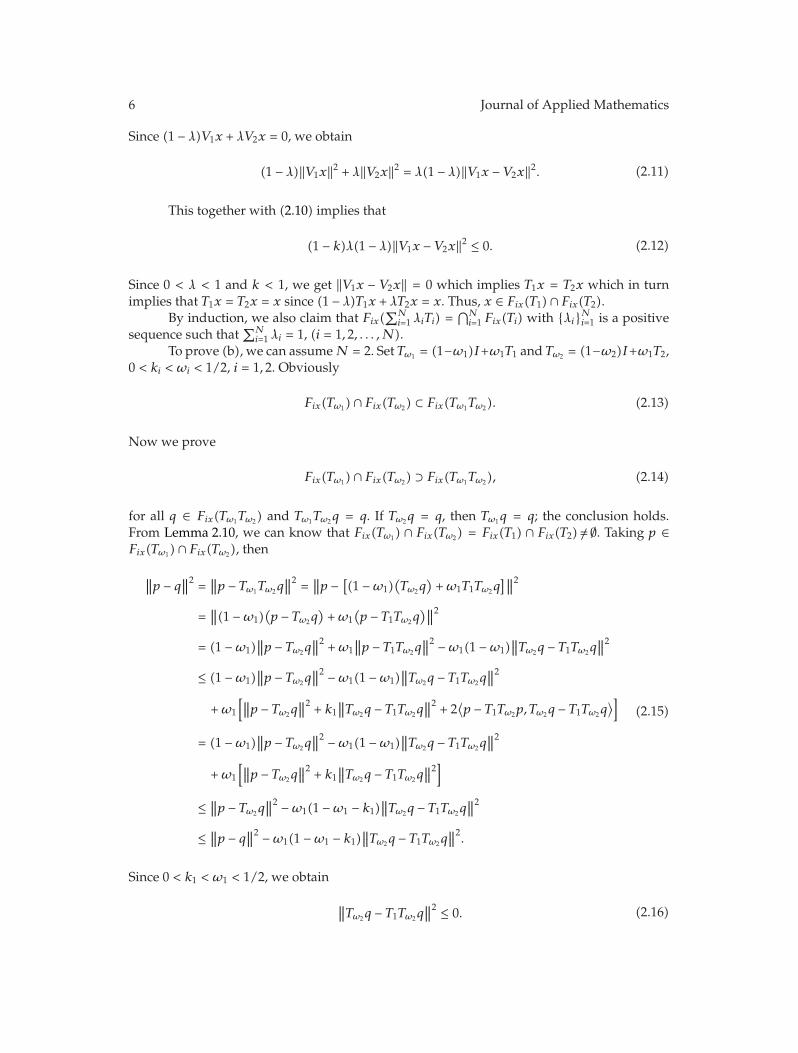
6 Journal of Applied Mathematics
Since (1 − λ)V1x + λV2x = 0, we obtain
(1 − λ)‖V1x‖2 + λ‖V2x‖2 = λ(1 − λ)‖V1x − V2x‖2. (2.11)
This together with (2.10) implies that
(1 − k)λ(1 − λ)‖V1x − V2x‖2 ≤ 0. (2.12)
Since 0 < λ < 1 and k < 1, we get ‖V1x − V2x‖ = 0 which implies T1x = T2x which in turnimplies that T1x = T2x = x since (1 − λ)T1x + λT2x = x. Thus, x ∈ Fix(T1) ∩ Fix(T2).
By induction, we also claim that Fix(∑N
i=1 λiTi) =⋂N
i=1 Fix(Ti) with {λi}Ni=1 is a positivesequence such that
∑Ni=1 λi = 1, (i = 1, 2, . . . ,N).
To prove (b), we can assume N = 2. Set Tω1 = (1−ω1)I+ω1T1 and Tω2 = (1−ω2)I+ω1T2,0 < ki < ωi < 1/2, i = 1, 2. Obviously
Fix(Tω1) ∩ Fix(Tω2) ⊂ Fix(Tω1Tω2). (2.13)
Now we prove
Fix(Tω1) ∩ Fix(Tω2) ⊃ Fix(Tω1Tω2), (2.14)
for all q ∈ Fix(Tω1Tω2) and Tω1Tω2q = q. If Tω2q = q, then Tω1q = q; the conclusion holds.From Lemma 2.10, we can know that Fix(Tω1) ∩ Fix(Tω2) = Fix(T1) ∩ Fix(T2)/= ∅. Taking p ∈Fix(Tω1) ∩ Fix(Tω2), then
∥∥p − q∥∥2 =
∥∥p − Tω1Tω2q∥∥2 =
∥∥p − [(1 −ω1)
(Tω2q
)+ω1T1Tω2q
]∥∥2
=∥∥(1 −ω1)
(p − Tω2q
)+ω1
(p − T1Tω2q
)∥∥2
= (1 −ω1)∥∥p − Tω2q
∥∥2 +ω1∥∥p − T1Tω2q
∥∥2 −ω1(1 −ω1)∥∥Tω2q − T1Tω2q
∥∥2
≤ (1 −ω1)∥∥p − Tω2q
∥∥2 −ω1(1 −ω1)∥∥Tω2q − T1Tω2q
∥∥2
+ω1
[∥∥p − Tω2q∥∥2 + k1
∥∥Tω2q − T1Tω2q∥∥2 + 2
⟨p − T1Tω2p, Tω2q − T1Tω2q
⟩]
= (1 −ω1)∥∥p − Tω2q
∥∥2 −ω1(1 −ω1)∥∥Tω2q − T1Tω2q
∥∥2
+ω1
[∥∥p − Tω2q∥∥2 + k1
∥∥Tω2q − T1Tω2q∥∥2]
≤ ∥∥p − Tω2q∥∥2 −ω1(1 −ω1 − k1)
∥∥Tω2q − T1Tω2q∥∥2
≤ ∥∥p − q∥∥2 −ω1(1 −ω1 − k1)
∥∥Tω2q − T1Tω2q∥∥2.
(2.15)
Since 0 < k1 < ω1 < 1/2, we obtain
∥∥Tω2q − T1Tω2q∥∥2 ≤ 0. (2.16)

Journal of Applied Mathematics 7
Namely, Tω2q = T1Tω2q, that is:
Tω2q ∈ Fix(T1) = Fix(Tω1), Tω2q = Tω1Tω2q. (2.17)
By induction, we also claim that the Lemma 2.11(b) holds.
Lemma 2.12. Let K be a closed convex subset of a real Hilbert space H, given x ∈ H and y ∈ K.Then y = PKx if and only if there holds the inequality
⟨x − y, y − z
⟩ ≥ 0, ∀z ∈ K. (2.18)
3. Cyclic Algorithm
In this section, we are concerned with the problem of finding a point p such that
p ∈N⋂
i=1
Fix(Tωi) =N⋂
i=1
Fix(Ti), N ≥ 1, (3.1)
where Tωi = (1 −ωi)I +ωiTi, {ωi}Ni=1 ∈ (0, 1/2] and {Ti}Ni=1 are ki-strictly pseudononspreadingmappings with ki ∈ [0, ωi), (i = 1, 2, . . . ,N), defined on a closed convex subset C in Hilbertspace H. Here Fix(Tωi) = {q ∈ C : Tωiq = q} is the set of fixed points of Ti, 1 ≤ i ≤ N.
Let H be a real Hilbert space, and let B : H → H be η-strongly monotone and ρ-Lipschitzian on H with ρ > 0, η > 0. Let 0 < μ < 2η/ρ2, 0 < γ < μ(η − (μρ2/2))/L = τ/L. LetN be a positive integer, and let Ti : H → H be a ki-strictly pseudononspreading mappingfor some ki ∈ [0, 1), (i = 1, 2, . . . ,N), such that
⋂Ni=1 Fix(Ti)/= ∅. We consider the problem of
finding p ∈ ⋂Ni=1 Fix(Ti) such that
⟨(γf − μB
)p, v − p
⟩ ≤ 0, ∀v ∈N⋂
i=1
Fix(Ti). (3.2)
Since⋂N
i=1 Fix(Ti) is a nonempty closed convex subset of H, VI (3.2) has a uniquesolution. The variational inequality has been extensively studied in literature; see, forexample, [12–16].
Remark 3.1. Let H be a real Hilbert space. Let B be a ρ-Lipschitzian and η-strongly monotoneoperator on H with ρ > 0, η > 0. Leting 0 < μ < 2η/ρ2 and leting S = (I − tμB) andμ(η − (μρ2/2)) = τ , then for ∀x, y ∈ H and t ∈ (0,min{1, 1/τ}), S is a contraction.
Proof. Consider
∥∥Sx − Sy∥∥2 =
∥∥(I − tμB)x − (I − tμB)y∥∥2
=⟨(I − tμB
)x − (
I − tμB)y,
(I − tμB
)x − (
I − tμB)y⟩
=∥∥x − y
∥∥2 + t2μ2∥∥Bx − By∥∥2 − 2tμ
⟨x − y, Bx − By
⟩

8 Journal of Applied Mathematics
≤ ‖x − y‖2 + t2μ2ρ2∥∥x − y∥∥2 − 2tμη
∥∥x − y
∥∥2
≤[
1 − 2tμ
(
η − μρ2
2
)]∥∥x − y
∥∥2
= (1 − 2tτ)∥∥x − y
∥∥2
≤ (1 − tτ)2∥∥x − y∥∥2
.
(3.3)
It follows that
∥∥Sx − Sy
∥∥ ≤ (1 − tτ)
∥∥x − y
∥∥. (3.4)
So S is a contraction.
Next, we consider the cyclic algorithm (1.15), respectively, for solving the variationalinequality over the set of the common fixed points of finite strictly pseudononspreadingmappings.
Lemma 3.2. Assume that {xn} is defined by (1.15); if p is solution of (3.2) with T : H → H beingstrictly pseudononspreading mapping and demiclosed and {yn} ⊂ H is a bounded sequence such that‖Tyn − yn‖ → 0, then
lim infn→∞
⟨(γf − μB
)p, yn − p
⟩ ≤ 0. (3.5)
Proof. By ‖Tyn − yn‖ → 0 and T : H → H demi-closed, we know that any weak clusterpoint of {yn} belongs to
⋂Ni=1 Fix(Ti). Furthermore, we can also obtain that there exists y and
a subsequence {ynj} of {yn} such that ynj ⇀ y as j → ∞ (hence y ∈ ⋂Ni=1 Fix(Ti)) and
lim infn→∞
⟨(γf − μB
)p, yn − p
⟩= lim
j→∞
⟨(γf − μB
)p, ynj − p
⟩. (3.6)
From (3.2), we can derive that
lim infn→∞
⟨(γf − μB
)p, yn − p
⟩=⟨(γf − μB
)p, y − p
⟩ ≤ 0. (3.7)
It is the desired result. In addition, the variational inequality (3.7) can be written as
⟨(I − μB + γf
)p − p, y − p
⟩ ≤ 0, y ∈N⋂
i=1
Fix(Ti). (3.8)

Journal of Applied Mathematics 9
So, by Lemma 2.12, it is equivalent to the fixed point equation
P⋂Ni=1 Fix(Ti)
(I − μB + γf
)p = p. (3.9)
Theorem 3.3. Let C be a nonempty closed convex subset of H and for 1 ≤ i ≤ N. Let Ti : H → Hbe ki-strictly pseudononspreading mappings for some ki ∈ [0, ωi), ωi ∈ (0, 1/2), (i = 1, 2, . . . ,N),and k = max{ki : 1 ≤ i ≤ N}. Let f be L-Lipschitz mapping on H with coefficient L > 0, and letB : H → H be η-strongly monotone and ρ-Lipschitzian on H with ρ > 0, η > 0. Let {αn} being asequence in (0,min{1, 1/τ}) satisfying the following conditions:
(c1) limn→∞αn = 0,
(c2)∑∞
n=0 αn = ∞.
Given x0 ∈ C, let {xn}∞n=1 be the sequence generated by the cyclic algorithm (1.15). Then {xn}converges strongly to the unique element p in
⋂Ni=1 Fix(Ti) verifying
p = P⋂Ni=1 Fix(Ti)
(I − μB + γf
)p, (3.10)
which equivalently solves the variational inequality problem (3.2).
Proof. Take a p ∈ ⋂Ni=1 Fix(Ti). Let Tωx = (1 −ω)x +ωTx and 0 < k < ω < 1/2. Then ∀x, y ∈ C,
we have
‖Tωx − Tωy‖2 = ω∥∥x − y
∥∥2 + (1 −ω)∥∥Tx − Ty
∥∥2 −ω(1 −ω)∥∥x − Tx − (
y − Ty)∥∥2
≤ ω∥∥x − y
∥∥2+(1 −ω)[∥∥x − y
∥∥2+k∥∥x − Tx − (
y − Ty)∥∥2+2〈x − Tx, y − Ty〉
]
−ω(1 −ω)∥∥x − Tx − (
y − Ty)∥∥2
=∥∥x − y
∥∥2+2(1 −ω)⟨x − Tx, y − Ty
⟩ − (1 −ω)(ω − k)∥∥x − Tx − (y − Ty)
∥∥2
≤ ∥∥x − y∥∥2+2(1 −ω)〈x − Tx, y − Ty〉
=∥∥x − y
∥∥2+2(1 −ω)
ω2
⟨x − Tωx, y − Tωy
⟩.
(3.11)
From p ∈ Fix(T) and (3.11), we also have
∥∥Tωxn − p∥∥ ≤ ∥∥xn − p
∥∥. (3.12)
Using (1.15) and (3.12), we obtain
∥∥xn+1 − p∥∥ =
∥∥αnγ(f(xn) − f
(p))
+ αn
(γf
(p) − p
)+(I − μαnB
)(Tω[n]xn − p
)∥∥
≤ αnγ∥∥f(xn) − f
(p)∥∥ + αn
∥∥γf(p) − p
∥∥ + (1 − αnτ)∥∥xn − p
∥∥,(3.13)

10 Journal of Applied Mathematics
which combined with (3.12) and ‖f(xn) − f(p)‖ ≤ L‖xn − p‖ amounts to
∥∥xn+1 − p
∥∥ ≤ (
1 − αn
(τ − γL
))∥∥xn − p∥∥ + αn
∥∥γf
(p) − p
∥∥. (3.14)
Putting M1 = max{‖x0 − p‖, ‖γf(p) − p‖}, we clearly obtain ‖xn − p‖ ≤ M1. Hence {xn} isbounded. We can also prove that the sequences {f(xn)} and {Tω[n]xn} are all bounded.
From (1.15) we obtain that
xn+1 − xn + αn
(μBxn − γf(xn)
)=(I − μαnB
)(Tω[n]xn − xn
), (3.15)
hence
⟨xn+1 − xn + αn
(μBxn − γf(xn)
), xn − p
⟩
= (1 − αn)⟨Tω[n]xn − xn, xn − p
⟩+ αn
⟨(I − μB
)(Tω[n]xn − xn
), xn − p
⟩
= (1 − αn)⟨Tω[n]xn − xn, xn − p
⟩+ αn
∥∥(I − μB)(Tω[n]xn − xn
)∥∥∥∥xn − p∥∥
= (1 − αn)⟨Tω[n]xn − xn, xn − p
⟩+ αn(1 − τ)
∥∥Tω[n]xn − xn
∥∥∥∥xn − p∥∥
= (1 − αn)⟨Tω[n]xn − xn, xn − p
⟩+ω[n]αn(1 − τ)
∥∥T[n]xn − xn
∥∥∥∥xn − p∥∥.
(3.16)
Moreover, by p ∈ ⋂Ni=1 Fix(Ti) and using Remark 2.5, we obtain
⟨xn − Tω[n]xn, xn − p
⟩ ≥ 12ω[n]
(1 − k[n]
)∥∥xn − T[n]xn
∥∥2, (3.17)
which combined with (3.16) entails
⟨xn+1 − xn + αn
(μB − γf
)xn, xn − p
⟩ ≤ −12ω[n]
(1 − k[n]
)(1 − αn)
∥∥xn − T[n]xn
∥∥2
+ω[n]αn(1 − τ)∥∥T[n]xn − xn
∥∥∥∥xn − p∥∥,
(3.18)
or equivalently
−〈xn − xn+1, xn − p〉
≤ −αn
⟨(μB − γf
)xn, xn − p
⟩ − 12ω[n]
(1 − k[n]
)(1 − αn)
∥∥xn − T[n]xn
∥∥2
+ω[n]αn(1 − τ)∥∥T[n]xn − xn
∥∥∥∥xn − p∥∥.
(3.19)
Furthermore, using the following classical equality
〈u, v〉 =12‖u‖2 − 1
2‖u − v‖2 +
12‖v‖2, ∀u, v ∈ C, (3.20)

Journal of Applied Mathematics 11
and setting Tn = 1/2‖xn − p‖2, we have
⟨xn − xn+1, xn − p
⟩= Tn − Tn+1 +
12‖xn − xn+1‖2. (3.21)
So (3.19) can be equivalently rewritten as
Tn+1 − Tn − 12‖xn − xn+1‖2 ≤ −αn〈
(μB − γf
)xn, xn − p〉
− 12ω[n]
(1 − k[n]
)(1 − αn)
∥∥xn − T[n]xn
∥∥2
+ω[n]αn(1 − τ)∥∥T[n]xn − xn
∥∥∥∥xn − p
∥∥.
(3.22)
Now using (3.15) again, we have
‖xn+1 − xn‖2 =∥∥αn(γf(xn) − μBxn) + (I − μαnB)(Tω[n]xn − xn)
∥∥2. (3.23)
Since B : H → H is η-strongly monotone and k-Lipschitzian on H, hence it is a classicalmatter to see that
‖xn+1 − xn‖2 ≤ 2α2n
∥∥γf(xn) − μBxn
∥∥2 + 2(1 − αnτ)2∥∥Tω[n]xn − xn
∥∥2, (3.24)
which by ‖Tω[n]xn − xn‖ = ω[n]‖xn − T[n]xn‖ and (1 − αnτ)2 ≤ (1 − αnτ) yields
12‖xn+1 − xn‖2 ≤ α2
n
∥∥γf(xn) − μBxn
∥∥2 + (1 − αnτ)ω2[n]
∥∥xn − T[n]xn
∥∥2. (3.25)
Then from (3.22) and (3.25), we have
Tn+1 − Tn +ω[n]
(12(1 − k[n]
)(1 − αn) −ω[n](1 − αnτ)
)∥∥xn − T[n]xn
∥∥2
≤αn
(αn
∥∥γf(xn) − μBxn
∥∥2 − ⟨(μB − γf
)xn, xn − p
⟩+ω[n](1 − τ)
∥∥T[n]xn − xn
∥∥∥∥xn − p∥∥).
(3.26)
The rest of the proof will be divided into two parts.Case 1. Suppose that there exists n0 such that {Tn}n≥n0
is nonincreasing. In thissituation, {Tn} is then convergent because it is also nonnegative (hence it is bounded frombelow), so that limn→∞(Tn+1 − Tn) = 0; hence, in light of (3.26) together with limn→∞αn = 0and the boundedness of {xn}, we obtain
limn→∞
∥∥xn − T[n]xn
∥∥ = 0. (3.27)

12 Journal of Applied Mathematics
It also follows from (3.26) that
Tn − Tn+1 ≥ αn
(−αn
∥∥γf(xn) − μBxn
∥∥2 +
⟨(μB − γf
)xn, xn − p
⟩
+ω[n](1 − τ)∥∥T[n]xn − xn
∥∥∥∥xn − p
∥∥).
(3.28)
Then, by∑∞
n=0 αn = ∞, we obviously deduce that
lim infn→∞
αn
(−αn
∥∥γf(xn) − μBxn
∥∥2 +
⟨(μB − γf
)xn, xn − p
⟩
+ω[n](1 − τ)∥∥T[n]xn − xn
∥∥∥∥xn − p
∥∥)≤ 0,
(3.29)
or equivalently (as αn‖γf(xn) − μBxn‖2 → 0)
lim infn→∞
⟨(μB − γf
)xn, xn − p
⟩ ≤ 0. (3.30)
Moreover, by Remark 1.2, we have
2(μη − γL
)Tn +⟨(μB − γf
)p, xn − p
⟩ ≤ ⟨(μB − γf
)xn, xn − p
⟩, (3.31)
which by (3.30) entails
lim infn→∞
⟨2(μη − γL
)Tn +(μB − γf
)p, xn − p
⟩ ≤ 0, (3.32)
hence, recalling that limn→∞Tn exists, we equivalently obtain
2(μη − γL
)limn→∞
Tn + lim infn→∞
⟨(μB − γf
)p, xn − p
⟩ ≤ 0, (3.33)
namely
2(μη − γL
)limn→∞
Tn ≤ −lim infn→∞
⟨(μB − γf
)p, xn − p
⟩. (3.34)
From (3.27) and Lemma 3.2, we obtain
lim infn→∞
⟨(μB − γf
)p, xn − p
⟩ ≥ 0, (3.35)
which yields limn→∞Tn = 0, so that {xn} converges strongly to p.

Journal of Applied Mathematics 13
Case 2. Suppose there exists a subsequence {Tnk}k≥0 of {Tn}n≥0 such that Tnk ≤ Tnk+1
for all k ≥ 0. In this situation, we consider the sequence of indices {δ(n)} as defined inLemma 2.8. It follows that Tδ(n+1) − Tδ(n) > 0, which by (3.26) amounts to
ω[n]
(12(1 − k[n]
)(1 − αδ(n)
) −ω[n](1 − αδ(n)τ
))∥∥xδ(n) − T[n]xδ(n)
∥∥2
< αδ(n)
(αδ(n)
∥∥γf
(xδ(n)
) − μBxδ(n)∥∥2 − ⟨(
μB − γf)xδ(n), xδ(n) − p
⟩
+ω[n](1 − τ)∥∥T[n]xδ(n) − xδ(n)
∥∥∥∥xδ(n) − p
∥∥).
(3.36)
By the boundedness of {xn} and limn→∞αn = 0, we immediately obtain
limn→∞
∥∥xδ(n) − T[n]xδ(n)
∥∥ = 0. (3.37)
Using (1.15), we have
‖xδ(n)+1 − xδ(n)‖ ≤ αδ(n)∥∥γf
(xδ(n)
) − μBxδ(n)∥∥ +
(1 − αδ(n)τ
)∥∥Tω[n]xδ(n) − xδ(n)∥∥
≤ αδ(n)∥∥γf
(xδ(n)
) − μBxδ(n)∥∥ +ω[n]
(1 − αδ(n)τ
)∥∥T[n]xδ(n) − xδ(n)∥∥,
(3.38)
which together with (3.37) and limn→∞αn = 0 yields
limn→∞
∥∥xδ(n)+1 − xδ(n)∥∥ = 0. (3.39)
Now by (3.36) we clearly have
αδ(n)∥∥γf(xδ(n)) − μBxδ(n)
∥∥2 +ω[n](1 − τ)∥∥T[n]xδ(n) − xδ(n)
∥∥∥∥xδ(n) − p∥∥
≥ ⟨(μB − γf
)xδ(n), xδ(n) − p
⟩,
(3.40)
which in the light of (3.31) yields
2(μη − γL
)Tδ(n) +⟨(μB − γf
)p, xδ(n) − p
⟩
≤ αδ(n)∥∥γf(xδ(n)) − μBxδ(n)
∥∥2 +ω[n](1 − τ)∥∥T[n]xδ(n) − x[n]
∥∥∥∥xδ(n) − p∥∥,
(3.41)
hence (as limn→∞αδ(n)‖γf(xδ(n)) − μBxδ(n)‖2 = 0 and (3.37)) it follows that
2(μη − γL
)lim supn→∞
Tδ(n) ≤ −lim infn→∞
⟨(μB − γf
)p, xδ(n) − p
⟩. (3.42)
From (3.37) and Lemma 3.2, we obtain
limn→∞
〈(μB − γf)p, xδ(n) − p〉 ≥ 0, (3.43)

14 Journal of Applied Mathematics
which by (3.42) yields lim supn→∞Tδ(n) = 0, so that limn→∞Tδ(n) = 0. Combining (3.39),we have limn→∞Tδ(n)+1 = 0. Then, recalling that Tn < Tδ(n)+1 (by Lemma 2.8), we getlimn→∞Tn = 0, so that xn → p strongly.
Taking ki = 0, we know that ki-strictly pseudononspreading mapping is nonspreadingmapping and i = n (mod N), 0 ≤ i ≤ N − 1. According to the proof Theorem 3.3, we obtainthe following corollary.
Corollary 3.4. Let C be a nonempty closed convex subset of H. Let Ti : C → C be nonspreadingmappings and ωi ∈ (0, 1/2), (i = 1, 2, . . . ,N). Let f be L-Lipschitz mapping on H with coefficientL > 0 and let B : H → H be η-strongly monotone and ρ-Lipschitzian on H with ρ > 0, η > 0. Let{αn} be a sequence in (0,min{1, 1/τ}) satisfying the following conditions:
(c1) limn→∞αn = 0,
(c2)∑∞
n=0 αn = ∞.
Given x0 ∈ C, let {xn}∞n=1 be the sequence generated by the cyclic algorithm (1.15). Then {xn}converges strongly to the unique element p in
⋂Ni=1 Fix(Ti) verifying
p = P⋂Ni=1 Fix(Ti)
(I − μB + γf
)p, (3.44)
which equivalently solves the variational inequality problem (3.2).
Acknowledgment
This work is supported in part by China Postdoctoral Science Foundation (Grant no.20100470783).
References
[1] F. E. Browder and W. V. Petryshyn, “Construction of fixed points of nonlinear mappings in Hilbertspace,” Journal of Mathematical Analysis and Applications, vol. 20, pp. 197–228, 1967.
[2] M. O. Osilike and F. O. Isiogugu, “Weak and strong convergence theorems for nonspreading-typemappings in Hilbert spaces,” Nonlinear Analysis: Theory, Methods & Applications, vol. 74, no. 5, pp.1814–1822, 2011.
[3] S. Iemoto and W. Takahashi, “Approximating common fixed points of nonexpansive mappings andnonspreading mappings in a Hilbert space,” Nonlinear Analysis: Theory, Methods & Applications, vol.71, no. 12, pp. e2082–e2089, 2009.
[4] K. Aoyama, “Halperns iteration for a sequence of quasinonexpansive type mappings,” NonlinearMathematics for Uncertainty and Its Applications, vol. 100, pp. 387–394, 2011.
[5] K. Aoyama and F. Kohsaka, “Fixed point and mean convergence theorems for a famliy of λ-hybridmappings,” Journal of Nonlinear Analysis and Optimization, vol. 2, no. 1, pp. 85–92, 2011.
[6] N. Petrot and R. Wangkeeree, “A general iterative scheme for strict pseudononspreading mappingrelated to optimization problem in Hilbert spaces,” Journal of Nonlinear Analysis and Optimization, vol.2, no. 2, pp. 329–336, 2011.
[7] G. L. Acedo and H.-K. Xu, “Iterative methods for strict pseudo-contractions in Hilbert spaces,”Nonlinear Analysis: Theory, Methods & Applications, vol. 67, no. 7, pp. 2258–2271, 2007.
[8] S. A. Naimpally and K. L. Singh, “Extensions of some fixed point theorems of Rhoades,” Journal ofMathematical Analysis and Applications, vol. 96, no. 2, pp. 437–446, 1983.
[9] T. L. Hicks and J. D. Kubicek, “On the Mann iteration process in a Hilbert space,” Journal ofMathematical Analysis and Applications, vol. 59, no. 3, pp. 498–504, 1977.

Journal of Applied Mathematics 15
[10] P.-E. Mainge, “The viscosity approximation process for quasi-nonexpansive mappings in Hilbertspaces,” Computers & Mathematics with Applications, vol. 59, no. 1, pp. 74–79, 2010.
[11] P.-E. Mainge, “Strong convergence of projected subgradient methods for nonsmooth and nonstrictlyconvex minimization,” Set-Valued Analysis, vol. 16, no. 7-8, pp. 899–912, 2008.
[12] S. Plubtieng and R. Punpaeng, “A new iterative method for equilibrium problems and fixedpoint problems of nonexpansive mappings and monotone mappings,” Applied Mathematics andComputation, vol. 197, no. 2, pp. 548–558, 2008.
[13] H.-K. Xu, “Iterative algorithms for nonlinear operators,” Journal of the London Mathematical SocietySecond Series, vol. 66, no. 1, pp. 240–256, 2002.
[14] H.-K. Xu, “Viscosity approximation methods for nonexpansive mappings,” Journal of MathematicalAnalysis and Applications, vol. 298, no. 1, pp. 279–291, 2004.
[15] H. K. Xu, “An iterative approach to quadratic optimization,” Journal of Optimization Theory andApplications, vol. 116, no. 3, pp. 659–678, 2003.
[16] L. C. Zeng, S. Schaible, and J. C. Yao, “Iterative algorithm for generalized set-valued stronglynonlinear mixed variational-like inequalities,” Journal of Optimization Theory and Applications, vol. 124,no. 3, pp. 725–738, 2005.

Hindawi Publishing CorporationJournal of Applied MathematicsVolume 2012, Article ID 683890, 10 pagesdoi:10.1155/2012/683890
Research ArticleA Note on Approximating Curve with1-Norm Regularization Method for the SplitFeasibility Problem
Songnian He1, 2 and Wenlong Zhu1, 2
1 College of Science, Civil Aviation University of China, Tianjin 300300, China2 Tianjin Key Laboratory for Advanced Signal Processing, Civil Aviation University of China,Tianjin 300300, China
Correspondence should be addressed to Songnian He, [email protected]
Received 21 March 2012; Accepted 6 June 2012
Academic Editor: Hong-Kun Xu
Copyright q 2012 S. He and W. Zhu. This is an open access article distributed under the CreativeCommons Attribution License, which permits unrestricted use, distribution, and reproduction inany medium, provided the original work is properly cited.
Inspired by the very recent results of Wang and Xu (2010), we study properties of the approximat-ing curve with 1-norm regularization method for the split feasibility problem (SFP). The conceptof the minimum-norm solution set of SFP in the sense of 1-norm is proposed, and the relationshipbetween the approximating curve and the minimum-norm solution set is obtained.
1. Introduction
Let C and Q be nonempty closed convex subsets of real Hilbert spaces H1 and H2, respective-ly. The problem under consideration in this paper is formulated as finding a point x satisfyingthe property:
x ∈ C, Ax ∈ Q, (1.1)
where A : H1 → H2 is a bounded linear operator. Problem (1.1), referred to by Censor andElfving [1] as the split feasibility problem (SFP), attracts many authors’ attention due to itsapplication in signal processing [1]. Various algorithms have been invented to solve it (see[2–13] and references therein).
Using the idea of Tikhonov’s regularization, Wang and Xu [14] studied the propertiesof the approximating curve for the SFP. They gave the concept of the minimum-normsolution of the SFP (1.1) and proved that the approximating curve converges strongly

2 Journal of Applied Mathematics
to the minimum-norm solution of the SFP (1.1). Together with some properties of thisapproximating curve, they introduced a modification of Byrne’s CQ algorithm [2] so thatstrong convergence is guaranteed and its limit is the minimum-norm solution of SFP (1.1).
In the practical application, H1 and H2 are often RN and R
M, respectively. Moreover,scientists and engineers are more willing to use 1-norm regularization method in thecalculation process (see, e.g., [15–18]). Inspired by the above results of Wang and Xu [14],we study properties of the approximating curve with 1-norm regularization method. We alsodefine the concept of the minimum-norm solution set of SFP (1.1) in the sense of 1-norm.The relationship between the approximating curve and the minimum-norm solution set isobtained.
2. Preliminaries
Let X be a normed linear space with norm ‖ · ‖, and let X∗ be the dual space of X. We usethe notation 〈x, f〉 to denote the value of f ∈ X∗ at x ∈ X. In particular, if X is a Hilbertspace, we will denote it by H, and 〈·, ·〉 and ‖ · ‖ are the inner product and its induced norm,respectively.
We recall some definitions and facts that are needed in our study.Let PC denote the projection from H onto a nonempty closed convex subset C of H;
that is,
PCx = arg miny∈C
‖x − y‖, x ∈ H. (2.1)
It is well known that PCx is characterized by the inequality
〈x − PCx, y − PCx〉 ≤ 0, ∀y ∈ C. (2.2)
Definition 2.1. Let ϕ : X → R ∪ {+∞} be a convex functional, x0 ∈ dom(ϕ) = {x ∈ X : ϕ(x) <+∞}. Set
∂ϕ(x0) ={ξ ∈ X∗ : ϕ(x) ≥ ϕ(x0) + 〈x − x0, ξ〉, ∀x ∈ X
}. (2.3)
If ∂ϕ(x0)/= ∅, ϕ is said to be subdifferentiable at x0 and ∂ϕ(x0) is called the subdifferential of ϕ atx0. For any ξ ∈ ∂ϕ(x0), we say ξ is a subgradient of ϕ at x0.
Lemma 2.2. There holds the following property:
∂(‖x‖) =⎧⎨
⎩
{x∗ ∈ X∗ : ‖x∗‖ = 1, 〈x, x∗〉 = ‖x‖}, x /= 0,
{x∗ ∈ X∗ : ‖x∗‖ ≤ 1}, x = 0,(2.4)
where ∂(‖x‖) denotes the subdifferential of the functional ‖x‖ at x ∈ X.
Proof. The process of the proof will be divided into two parts.

Journal of Applied Mathematics 3
Case 1. In the case of x = 0, for any x∗ ∈ X∗ such that ‖x∗‖ ≤ 1 and any y ∈ X, there holds theinequality
‖y‖ ≥ 〈y, x∗〉 = ‖x‖ + 〈y − x, x∗〉, (2.5)
so we have x∗ ∈ ∂(‖x‖), and thus,
{x∗ ∈ X∗ : ‖x∗‖ ≤ 1} ⊂ ∂(‖x‖). (2.6)
Conversely, for any x∗ ∈ ∂(‖x‖), we have from the definition of subdifferential that
‖y‖ ≥ ‖x‖ + ⟨y − x, x∗⟩ =⟨y, x∗⟩, ∀y ∈ X,
‖y‖ = ‖ − y‖ ≥ 〈−y, x∗〉 = −〈y, x∗〉.(2.7)
Consequently,
∣∣〈y, x∗〉∣∣ ≤ ‖y‖, ∀y ∈ X, (2.8)
and this implies that ‖x∗‖ ≤ 1. Thus, we have verified that
∂(‖x‖) ⊂ {x∗ ∈ X∗ : ‖x∗‖ ≤ 1}. (2.9)
Combining (2.6) and (2.9), we immediately obtain
∂(‖x‖) = {x∗ ∈ X∗ : ‖x∗‖ ≤ 1}. (2.10)
Case 2. If x /= 0, for any x∗ ∈ {x∗ ∈ X∗ : ‖x∗‖ = 1, 〈x, x∗〉 = ‖x‖}, we obviously have
〈y − x, x∗〉 = 〈y, x∗〉 − ‖x‖ ≤ ‖y‖ − ‖x‖, ∀y ∈ X, (2.11)
which means that x∗ ∈ ∂(‖x‖), and thus,
{x∗ ∈ X∗ : ‖x∗‖ = 1, 〈x, x∗〉 = ‖x‖} ⊂ ∂(‖x‖). (2.12)
Conversely, if x∗ ∈ ∂(‖x‖), we have
〈−x, x∗〉 ≤ 0 − ‖x‖ = −‖x‖, 〈x, x∗〉 ≤ 2‖x‖ − ‖x‖ = ‖x‖; (2.13)
hence,
〈x, x∗〉 = ‖x‖. (2.14)

4 Journal of Applied Mathematics
On the other hand, using (2.14), we get
‖y‖ ≥ ‖x‖ + 〈y − x, x∗〉 = ‖x‖ + 〈y, x∗〉 − 〈x, x∗〉 = 〈y, x∗〉, ∀y ∈ X, (2.15)
and consequently,
∥∥y∥∥ =∥∥−y∥∥ ≥ ‖x‖ + ⟨−y − x, x∗⟩
= ‖x‖ − ⟨y, x∗⟩ − 〈x, x∗〉= −⟨y, x∗⟩;
(2.16)
that is,
−‖y‖ ≤ 〈y, x∗〉. (2.17)
Equation (2.17) together with (2.15) implies that
∣∣⟨y, x∗⟩∣∣ ≤ ‖y‖, ∀y ∈ X; (2.18)
hence, ‖x∗‖ ≤ 1. Note that (2.14) implies that ‖x∗‖ ≥ 〈x, x∗〉/‖x‖ = 1; we assert that
‖x∗‖ = 1. (2.19)
Thus we have from (2.14) and (2.19) that
{x∗ ∈ X∗ : ‖x∗‖ = 1, 〈x, x∗〉 = ‖x‖} ⊃ ∂(‖x‖). (2.20)
The proof is finished by combining (2.12) and (2.20).
‖ · ‖∞ and ‖ · ‖1 will stand for ∞-norm and 1-norm of any Euclidean space; respectively,that is, for any x = (x1, x2, . . . , xl) ∈ R
l, we have
‖x‖∞ = max1≤j≤l
∣∣xj
∣∣, ‖x‖1 =l∑
j=1
∣∣xj
∣∣. (2.21)
Corollary 2.3. In l-dimensional Euclidean space Rl, there holds the following result:
∂(‖x‖1) =
⎧⎨
⎩
{ξ ∈ R
l : ‖ξ‖∞ = 1, 〈x, ξ〉 = ‖x‖1}, x /= 0,
{ξ ∈ R
l : ‖ξ‖∞ ≤ 1}, x = 0,
=
⎧⎪⎨
⎪⎩
{ξ ∈ R
l : ξi =xi
|xi| , if xi /= 0; ξi ∈ [−1, 1], if xi = 0}, x /= 0,
{ξ ∈ R
l : ‖ξ‖∞ ≤ 1}, x = 0.
(2.22)

Journal of Applied Mathematics 5
LetH be a Hilbert space and f : H → R a functional. Recall that
(i) f is convex if f(λx + (1 − λ)y) ≤ λf(x) + (1 − λ)f(y), for all 0 < λ < 1, for all x, y ∈ H;
(ii) f is strictly convex if f(λx + (1 − λ)y) < λf(x) + (1 − λ)f(y), for all 0 < λ < 1, for allx, y ∈ H with x /=y;
(iii) f is coercive if f(x) → ∞ whenever ‖x‖ → ∞. See [19] for more details about convexfunctions.
The following lemma gives the optimality condition for the minimizer of a convexfunctional over a closed convex subset.
Lemma 2.4 (see [20]). Let H be a Hilbert space and C a nonempty closed convex subset of H. Letf : H → R be a convex and subdifferentiable functional. Then x ∈ C is a solution of the problem
minx∈C
f(x) (2.23)
if and only if there exists some ξ ∈ ∂f(x) satisfying the following optimality condition:
〈ξ, v − x〉 ≥ 0, ∀v ∈ C. (2.24)
3. Main Results
It is well known that SFP (1.1) is equivalent to the minimization problem
minx∈C
∥∥(I − PQ
)Ax∥∥2
. (3.1)
Using the idea of Tikhonov’s regularization method, Wang and Xu [14] studied the mini-mization problem in Hilbert spaces:
minx∈C
∥∥(I − PQ
)Ax∥∥2 + α‖x‖2, (3.2)
where α > 0 is the regularization parameter.In what follows, H1 and H2 in SFP (1.1) are restricted to R
N and RM, respectively,
and ‖ · ‖ will stand for the usual 2-norm of any Euclidean space Rl; that is, for any x =
(x1, x2, . . . , xl) ∈ Rl,
‖x‖ =√x2
1 + · · · + x2l. (3.3)
Inspired by the above work of Wang and Xu, we study properties of the approximating curvewith 1-norm regularization scheme for the SFP, that is, the following minimization problem:
minx∈C
12∥∥(I − PQ
)Ax∥∥2 + α‖x‖1, (3.4)

6 Journal of Applied Mathematics
where α > 0 is the regularization parameter. Let
fα(x) =12∥∥(I − PQ
)Ax∥∥2 + α‖x‖1. (3.5)
It is easy to see that fα is convex and coercive, so problem (3.4) has at least one solution.However, the solution of problem (3.4) may not be unique since fα is not necessarily strictlyconvex. Denote by Sα the solution set of problem (3.4); thus we can assert that Sα is anonempty closed convex set but may contain more than one element. The following simpleexample illustrates this fact.
Example 3.1. Let C = {(x, y) : x + y = 1}, Q = {(x, y) : x + y = 1/2} and
A =
⎛
⎜⎜⎝
12
0
012
⎞
⎟⎟⎠. (3.6)
Then A : R2 → R
2 is a bounded linear operator. Obviously, Sα = {(x, y) : x + y = 1, x ≥ 0, y ≥0} and it contains more than one element.
Proposition 3.2. For any α > 0, xα ∈ Sα if and only if there exists some ξ ∈ ∂(‖x‖1) satisfying thefollowing inequality:
⟨A∗(I − PQ
)Axα + αξ, v − xα
⟩ ≥ 0, ∀v ∈ C. (3.7)
Proof. Let
f(x) =12∥∥(I − PQ
)Ax∥∥2
, (3.8)
then
fα(x) = f(x) + α‖x‖1. (3.9)
Since f is convex and differentiable with gradient
∇f(x) = A∗(I − PQ
)Ax, (3.10)
fα is convex, coercive, and subdifferentiable with the subdifferential
∂fα(x) = ∂f(x) + α∂(‖x‖1); (3.11)
that is,
∂fα(x) = A∗(I − PQ
)Ax + α∂(‖x‖1). (3.12)
By Corollary 2.3 and Lemma 2.4, the proof is finished.

Journal of Applied Mathematics 7
Theorem 3.3. Denote by xα an arbitrary element of Sα, then the following assertions hold:
(i) ‖xα‖1 is decreasing for α ∈ (0,∞);
(ii) ‖(I − PQ)Axα‖ is increasing for α ∈ (0,∞).
Proof. Let α > β > 0, for any xα ∈ Sα, xβ ∈ Sβ. We immediately obtain
12∥∥(I − PQ
)Axα
∥∥2 + α‖xα‖1 ≤ 1
2∥∥(I − PQ
)Axβ
∥∥2 + α
∥∥xβ
∥∥
1, (3.13)
12∥∥(I − PQ
)Axβ
∥∥2 + β
∥∥xβ
∥∥
1 ≤ 12∥∥(I − PQ
)Axα
∥∥2 + β‖xα‖1. (3.14)
Adding up (3.13) and (3.14) yields
α‖xα‖1 + β∥∥xβ
∥∥1 ≤ α
∥∥xβ
∥∥1 + β‖xα‖1, (3.15)
which implies ‖xα‖1 ≤ ‖xβ‖1. Hence (i) holds.Using (3.14) again, we have
12∥∥(I − PQ
)Axβ
∥∥2 ≤ 12∥∥(I − PQ
)Axα
∥∥2 + β(‖xα‖1 −
∥∥xβ
∥∥1
), (3.16)
which together with (i) implies
∥∥(I − PQ
)Axβ
∥∥2 ≤ ∥∥(I − PQ
)Axα
∥∥2, (3.17)
and hence (ii) holds.
Let F = C ∩A−1(Q), where A−1(Q) = {x ∈ RN : Ax ∈ Q}. In what follows, we assume
that F /= ∅; that is, the solution set of SFP (1.1) is nonempty. The fact that F is nonempty closedconvex set thus allows us to introduce the concept of minimum-norm solution of SFP (1.1) inthe sense of norm ‖ · ‖ (induced by the inner product).
Definition 3.4 (see [14]). An element x† ∈ F is said to be the minimum-norm solution of SFP(1.1) in the sense of norm ‖ · ‖ if ‖x†‖ = infx∈F‖x‖. In other words, x† is the projection of theorigin onto the solution set F of SFP (1.1). Thus there exists only one minimum-norm solutionof SFP (1.1) in the sense of norm ‖ · ‖, which is always denoted by x†.
We can also give the concept of minimum-norm solution of SFP (1.1) in other senses.
Definition 3.5. An element x ∈ F is said to be a minimum-norm solution of SFP (1.1) in the senseof 1-norm if ‖x‖1 = infx∈F‖x‖1. We use F1 to stand for all minimum-norm solutions of SFP(1.1) in the sense of 1-norm and F1 is called the minimum-norm solution set of SFP (1.1) inthe sense of 1-norm.
Obviously, F1 is a closed convex subset of F. Moreover, it is easy to see that F1 /= ∅.Indeed, taking a sequence {xn} ⊂ F such that ‖xn‖1 → infx∈F‖x‖1 as n → ∞, then {xn}

8 Journal of Applied Mathematics
is bounded. There exists a convergent subsequence {xnk} of {xn}. Set x = limk→∞xnk , thenx ∈ F since F is closed. On the other hand, using lower semicontinuity of the norm, we have
‖x‖ ≤ limk→∞
‖xnk‖ = infx∈F
‖x‖1, (3.18)
and this implies that x ∈ F1.However, F1 may contain more than one elements, in general (see Example 3.1, F1 =
{(x, y) : x + y = 1, x, y ≥ 0}).
Theorem 3.6. Let α > 0 and xα ∈ Sα. Thenω(xα) ⊂ F1, whereω(xα) = {x : ∃{xαk} ⊂ {xα}, xαk →x weakly}.
Proof. Taking x ∈ F1 arbitrarily, for any α ∈ (0,∞), we always have
12∥∥(I − PQ
)Axα
∥∥2 + α‖xα‖1 ≤ 12∥∥(I − PQ
)Ax∥∥2 + α‖x‖1. (3.19)
Since x is a solution of SFP (1.1), ‖(I − PQ)Ax‖ = 0. This implies that
12∥∥(I − PQ)Axα
∥∥2 + α‖xα‖1 ≤ α‖x‖1, (3.20)
then,
‖xα‖1 ≤ ‖x‖1; (3.21)
thus {xα} is bounded.Take ω ∈ ω(xα) arbitrarily, then there exists a sequence {αn} such that αn → 0 and
xαn → ω as n → ∞. Put xαn = xn. By Proposition 3.2, we deduce that there exists some ξn ∈∂(‖xn‖1) such that
⟨A∗(I − PQ
)Axn + αnξn, x − xn
⟩ ≥ 0. (3.22)
This implies that
⟨(I − PQ
)Axn,A(x − xn)
⟩ ≥ αn〈ξn, xn − x〉. (3.23)
Since Ax ∈ Q, the characterizing inequality (2.2) gives
⟨(I − PQ
)Axn,Ax − PQ(Axn)
⟩ ≤ 0, (3.24)
then,
∥∥(I − PQ
)Axn
∥∥2 ≤ ⟨(I − PQ
)Axn,A(xn − x)
⟩. (3.25)

Journal of Applied Mathematics 9
Combining (3.23) and (3.25), we have∥∥(I − PQ
)Axn
∥∥2 ≤ αn〈ξn, x − xn〉
≤ αn‖ξn‖∞‖x − xn‖1
≤ 2αn‖x‖1.
(3.26)
Consequently, we get
limn→∞
∥∥(I − PQ
)Axn
∥∥ = 0. (3.27)
Furthermore, noting the fact that xn → ω and I − PQ and A are all continuous operators, wehave (I − PQ)Aω = 0; that is, Aω ∈ Q; thus, ω ∈ F. Since x is a minimum-norm solution ofSFP (1.1) in the sense of 1-norm, using (3.21) again, we get
‖ω‖1 ≤ lim infn→∞
‖xn‖1 ≤ ‖x‖1 = min{‖x‖1 : x ∈ F}. (3.28)
Thus we can assert that ω ∈ F1 and this completes the proof.
Corollary 3.7. If F1 contains only one element x, then xα → x, (α → 0).
Remark 3.8. It is worth noting that the minimum-norm solution of SFP (1.1) in the sense ofnorm ‖ · ‖ is very different from the minimum-norm solution of SFP (1.1) in the sense of1-norm. In fact, x† may not belong to F1! The following simple example shows this fact.
Example 3.9. Let C = {(x, y) : x + 2y ≥ 2, x ≥ 0, y ≥ 0}, Q = {(x, y) : x + y = 1, x ≥ 0, y ≥ 0},and
A =
⎛
⎝12
0
0 1
⎞
⎠. (3.29)
It is not hard to see that A : R2 → R
2 is a bounded linear operator and A(x, y)T = ((1/2)x,y)T , for all (x, y) ∈ C. Obviously, F = {(x, y) : x + 2y = 2, x ≥ 0, y ≥ 0}, x† = (2/5, 4/5), butF1 = {(0, 1)}. Hence, x† ∈ F \ F1.
Acknowledgments
This work was supported by the Fundamental Research Funds for the Central Universities(ZXH2012K001) and in part by the Foundation of Tianjin Key Lab for Advanced SignalProcessing. W. Zhu was also supported by the Postgraduate Science and TechnologyInnovation Funds (YJSCX12-22).
References
[1] Y. Censor and T. Elfving, “A multiprojection algorithm using Bregman projections in a productspace,” Numerical Algorithms, vol. 8, no. 2–4, pp. 221–239, 1994.

10 Journal of Applied Mathematics
[2] Y. Yao, R. Chen, G. Marino, and Y. C. Liou, “Applications of fixed point and optimization methods tothe multiple-sets split feasibility problem,” Journal of Applied Mathematics, vol. 2012, Article ID 927530,21 pages, 2012.
[3] C. Byrne, “Iterative oblique projection onto convex sets and the split feasibility problem,” InverseProblems, vol. 18, no. 2, pp. 441–453, 2002.
[4] C. Byrne, “A unified treatment of some iterative algorithms in signal processing and imagereconstruction,” Inverse Problems, vol. 20, no. 1, pp. 103–120, 2004.
[5] B. Qu and N. Xiu, “A note on the CQ algorithm for the split feasibility problem,” Inverse Problems, vol.21, no. 5, pp. 1655–1665, 2005.
[6] H. K. Xu, “A variable Krasnosel’skii-Mann algorithm and the multiple-set split feasibility problem,”Inverse Problems, vol. 22, no. 6, pp. 2021–2034, 2006.
[7] Q. Yang, “The relaxed CQ algorithm solving the split feasibility problem,” Inverse Problems, vol. 20,no. 4, pp. 1261–1266, 2004.
[8] Q. Yang and J. Zhao, “Generalized KM theorems and their applications,” Inverse Problems, vol. 22, no.3, pp. 833–844, 2006.
[9] Y. Yao, J. Wu, and Y. C. Liou, “Regularized methods for the split feasibility problem,” Abstract andApplied Analysis, vol. 2012, Article ID 140679, 15 pages, 2012.
[10] X. Yu, N. Shahzad, and Y. Yao, “Implicit and explicit algorithms for solving the split feasibilityproblem ,” Optimization Letters. In press.
[11] F. Wang and H. K. Xu, “Cyclic algorithms for split feasibility problems in Hilbert spaces,” NonlinearAnalysis, Theory, Methods and Applications, vol. 74, no. 12, pp. 4105–4111, 2011.
[12] H. K. Xu, “Averaged mappings and the gradient-projection algorithm,” Journal of Optimization Theoryand Applications, vol. 150, no. 2, pp. 360–378, 2011.
[13] H. K. Xu, “Iterative methods for the split feasibility problem in infinite-dimensional Hilbert spaces,”Inverse Problems, vol. 26, no. 10, Article ID 105018, 2010.
[14] H. K. Xu and F. Wang, “Approximating curve and strong convergence of the CQ algorithm for thesplit feasibility problem,” Journal of Inequalities and Applications, vol. 2010, Article ID 102085, 13 pages,2010.
[15] M. R. Kunz, J. H. Kalivas, and E. Andries, “Model updating for spectral calibration maintenance andtransfer using 1-norm variants of tikhonov regularization,” Analytical Chemistry, vol. 82, no. 9, pp.3642–3649, 2010.
[16] X. Nan, N. Wang, P. Gong, C. Zhang, Y. Chen, and D. Wilkins, “Gene selection using 1-normregulariza-tion for multi-class microarray data,” in Proceedings of the IEEE International Conference onBioinformatics and Biomedicine (BIBM ’10), pp. 520–524, December 2010.
[17] X. Nan, Y. Chen, D. Wilkins, and X. Dang, “Learning to rank using 1-norm regularization and convexhull reduction,” in Proceedings of the 48th Annual Southeast Regional Conference (ACMSE ’10), Oxford,Miss, USA, April 2010.
[18] H. W. Park, M. W. Park, B. K. Ahn, and H. S. Lee, “1-Norm-based regularization scheme for systemidentification of structures with discontinuous system parameters,” International Journal for NumericalMethods in Engineering, vol. 69, no. 3, pp. 504–523, 2007.
[19] J. P. Aubin, Optima and Equilibria: An Introduction to Nonliear Analysis, vol. 140 of Graduate Texts inMathematics, Springer, Berlin, Germany, 1993.
[20] H. W. Engl, M. Hanke, and A. Neubauer, Regularization of Inverse Problems, vol. 375 of Mathematics andIts Applications, Kluwer Academic, Dordrecht, The Netherlands, 1996.

Hindawi Publishing CorporationJournal of Applied MathematicsVolume 2012, Article ID 174318, 20 pagesdoi:10.1155/2012/174318
Research ArticleGeneral Iterative Algorithms for Hierarchical FixedPoints Approach to Variational Inequalities
Nopparat Wairojjana and Poom Kumam
Department of Mathematics, Faculty of Science, King Mongkut’s University of Technology Thonburi(KMUTT), Bangmod, Bangkok 10140, Thailand
Correspondence should be addressed to Poom Kumam, [email protected]
Received 24 March 2012; Accepted 16 May 2012
Academic Editor: Zhenyu Huang
Copyright q 2012 N. Wairojjana and P. Kumam. This is an open access article distributed underthe Creative Commons Attribution License, which permits unrestricted use, distribution, andreproduction in any medium, provided the original work is properly cited.
This paper deals with new methods for approximating a solution to the fixed point problem; findx ∈ F(T), where H is a Hilbert space, C is a closed convex subset of H, f is a ρ-contraction fromC into H, 0 < ρ < 1, A is a strongly positive linear-bounded operator with coefficient γ > 0,0 < γ < γ/ρ, T is a nonexpansive mapping on C, and PF(T) denotes the metric projection on the setof fixed point of T . Under a suitable different parameter, we obtain strong convergence theorems byusing the projection method which solves the variational inequality 〈(A−γf)x+τ(I−S)x, x−x〉 ≥ 0for x ∈ F(T), where τ ∈ [0,∞). Our results generalize and improve the corresponding results ofYao et al. (2010) and some authors. Furthermore, we give an example which supports our maintheorem in the last part.
1. Introduction
Throughout this paper, we assume that H is a real Hilbert space where inner product andnorm are denoted by 〈·, ·〉 and ‖ · ‖, respectively, and let C be a nonempty closed convexsubset of H. A mapping T : C → C is called nonexpansive if
∥∥Tx − Ty∥∥ ≤ ∥∥x − y
∥∥, ∀x, y ∈ C. (1.1)
We use F(T) to denote the set of fixed points of T , that is, F(T) = {x ∈ C : Tx = x}. It isassumed throughout the paper that T is a nonexpansive mapping such that F(T)/= ∅.
Recall that a mapping f : C → H is a contraction on C if there exists a constantρ ∈ (0, 1) such that
∥∥f(x) − f
(y)∥∥ ≤ ρ
∥∥x − y∥∥, ∀x, y ∈ C. (1.2)

2 Journal of Applied Mathematics
A mapping A : H → H is called a strongly positive linear bounded operator on H if thereexists a constant γ > 0 with property
〈Ax, x〉 ≥ γ‖x‖2, ∀x ∈ H. (1.3)
A mapping M : H → H is called a strongly monotone operator with α if
⟨x − y,Mx −My
⟩ ≥ α∥∥x − y
∥∥2, ∀x, y ∈ H, (1.4)
and M is called a monotone operator if
⟨x − y,Mx −My
⟩ ≥ 0, ∀x, y ∈ H. (1.5)
We easily prove that the mapping (I−T) is monotone operator, if T is nonexpansive mapping.The metric (or nearest point) projection from H onto C is mapping PC[·] : H → C which
assigns to each point x ∈ C the unique point PC[x] ∈ C satisfying the property
‖x − PC[x]‖ = infy∈C
∥∥x − y∥∥ =: d(x,C). (1.6)
The variational inequality for a monotone operator, M : H → H over C, is to find apoint in
VI(C,M) := {x ∈ C : 〈x − x,Mx〉 ≥ 0, ∀x ∈ C}. (1.7)
A hierarchical fixed point problem is equivalent to the variational inequality for amonotone operator over the fixed point set. Moreover, to find a hierarchically fixed pointof a nonexpansive mapping T with respect to another nonexpansive mapping S, namely, wefind x ∈ F(T) such that
〈x − x, (I − S)x〉 ≥ 0, ∀x ∈ F(T). (1.8)
Iterative methods for nonexpansive mappings have recently been applied to solve aconvex minimization problem; see, for example, [1–5] and the references therein. A typicalproblem is to minimize a quadratic function over the set of the fixed points of a nonexpansivemapping on a real Hilbert space H:
minx∈F(T)
12〈Ax, x〉 − 〈x, b〉, (1.9)
where b is a given point in H. In [5], it is proved that the sequence {xn} defined by theiterative method below, with the initial guess x0 ∈ H chosen arbitrarily,
xn+1 = (I − αnA)Txn + αnb, n ≥ 0, (1.10)

Journal of Applied Mathematics 3
converges strongly to the unique solution of the minimization problem (1.9) provided thesequence {αn} of parameters satisfies certain appropriate conditions.
On the other hand, Moudafi [6] introduced the viscosity approximation methodfor nonexpansive mappings (see [7] for further developments in both Hilbert and Banachspaces). Starting with an arbitrary initial x0 ∈ H, define a sequence {xn} recursively by
xn+1 = σnf(xn) + (1 − σn)Txn, n ≥ 0, (1.11)
where {σn} is a sequence in (0, 1). It is proved in [6, 7] that under certain appropriateconditions imposed on {σn}, the sequence {xn} generated by (1.11) strongly converges tothe unique solution x∗ in C of the variational inequality
⟨(I − f
)x∗, x − x∗⟩ ≥ 0, x ∈ C . (1.12)
In 2006, Marino and Xu [8] introduced a general iterative method for nonexpansivemapping. Starting with an arbitrary initial x0 ∈ H, define a sequence {xn} recursively by
xn+1 = εnγf(xn) + (I − εnA)Txn, n ≥ 0 . (1.13)
They proved that if the sequence {εn} of parameters satisfies appropriate conditions, then thesequence {xn} generated by (1.13) strongly converges to the unique solution x = PF(T)(I −A+γf)x of the variational inequality
⟨(A − γf
)x, x − x
⟩ ≥ 0, ∀x ∈ F(T), (1.14)
which is the optimality condition for the minimization problem
minx∈F(T)
12〈Ax, x〉 − h(x), (1.15)
where h is a potential function for γf (i.e., h′(x) = γf(x) for x ∈ H).In 2010, Yao et al. [9] introduced an iterative algorithm for solving some hierarchical
fixed point problem, starting with an arbitrary initial guess x0 ∈ C, define a sequence {xn}iteratively by
yn = βnSxn +(1 − βn
)xn,
xn+1 = PC
[αnf(xn) + (1 − αn)Tyn
], ∀n ≥ 1.
(1.16)
They proved that if the sequences {αn} and {βn} of parameters satisfies appropriateconditions, then the sequence {xn} generated by (1.16) strongly converges to the uniquesolution z in H of the variational inequality
z ∈ F(T),⟨(I − f
)z, x − z
⟩ ≥ 0, ∀x ∈ F(T). (1.17)

4 Journal of Applied Mathematics
In this paper we will combine the general iterative method (1.13) with the iterativealgorithm (1.16) and consider the following iterative algorithm:
yn = βnSxn +(1 − βn
)xn,
xn+1 = PC
[αnγf(xn) + (I − αnA)Tyn
], ∀n ≥ 1.
(1.18)
We will prove in Section 3 that if the sequences {αn} and {βn} of parameters satisfyappropriate conditions and limn→∞(βn/αn) = τ ∈ (0,∞) then the sequence {xn} generated by(1.18) converges strongly to the unique solution x in H of the following variational inequality
x ∈ F(T),⟨
1τ
(A − γf
)x + (I − S)x, x − x
⟩≥ 0, ∀x ∈ F(T). (1.19)
In particular, if we take τ = 0, under suitable difference assumptions on parameter, then thesequence {xn} generated by (1.18) converges strongly to the unique solution x in H of thefollowing variational inequality
x ∈ F(T),⟨(A − γf
)x, x − x
⟩ ≥ 0, ∀x ∈ F(T). (1.20)
Our results improve and extend the recent results of Yao et al. [9] and some authors.Furthermore, we give an example which supports our main theorem in the last part.
2. Preliminaries
This section collects some lemma which can be used in the proofs for the main results in thenext section. Some of them are known, others are not hard to derive.
Lemma 2.1 (Browder [10]). Let H be a Hilbert space, C be a closed convex subset of H, and T :C → C be a nonexpansive mapping with F(T)/= ∅. If {xn} is a sequence in C weakly converging to xand if {(I − T)xn} converges strongly to y, then (I − T)x = y; in particular, if y = 0 then x ∈ F(T).
Lemma 2.2. Let x ∈ H and z ∈ C be any points. Then one has the following:
(1) That z = PC[x] if and only if there holds the relation:
⟨x − z, y − z
⟩ ≤ 0, ∀y ∈ C. (2.1)
(2) That z = PC[x] if and only if there holds the relation:
‖x − z‖2 ≤ ∥∥x − y∥∥2 − ∥∥y − z
∥∥2, ∀y ∈ C. (2.2)

Journal of Applied Mathematics 5
(3) There holds the relation:
⟨PC[x] − PC
[y], x − y
⟩ ≥ ∥∥PC[x] − PC
[y]∥∥2
, ∀x, y ∈ H. (2.3)
Consequently, PC is nonexpansive and monotone.
Lemma 2.3 (Marino and Xu [8]). Let H be a Hilbert space, C be a closed convex subset of H,f : C → H be a contraction with coefficient 0 < ρ < 1, and T : C → C be nonexpansive mapping.
Let A be a strongly positive linear bounded operator on a Hilbert spaceH with coefficient−γ> 0. Then,
for 0 < γ <−γ /ρ, for x, y ∈ C,
(1) the mapping (I − f) is strongly monotone with coefficient (1 − ρ), that is,
⟨x − y,
(I − f
)x − (
I − f)y⟩ ≥ (
1 − ρ)∥∥x − y
∥∥2
, (2.4)
(2) the mapping (A − γf) is strongly monotone with coefficient−γ −γρ that is
⟨x − y,
(A − γf
)x − (
A − γf)y⟩ ≥
(−γ −γρ
)∥∥x − y∥∥2
. (2.5)
Lemma 2.4 (Xu [4]). Assume that {an} is a sequence of nonnegative numbers such that
an+1 ≤ (1 − γn
)an + δn, ∀n ≥ 0, (2.6)
where {γn} is a sequence in (0, 1) and {δn} is a sequence in R such that
(1)∑∞
n=1 γn = ∞,
(2) lim supn→∞(δn/γn) ≤ 0 or∑∞
n=1 |δn| < ∞. Then limn→∞an = 0.
Lemma 2.5 (Marino and Xu [8]). Assume A is a strongly positive linear bounded operator on a
Hilbert spaceH with coefficient−γ> 0 and 0 < α ≤ ‖A‖−1. Then ‖I − αA‖ ≤ 1 − α
−γ .
Lemma 2.6 (Acedo and Xu [11]). Let C be a closed convex subset of H. Let {xn} be a boundedsequence inH. Assume that
(1) The weak ω-limit set ωw(xn) ⊂ C,
(2) For each z ∈ C, limn→∞‖xn − z‖ exists. Then {xn} is weakly convergent to a point in C.
Notation. We use → for strong convergence and ⇀ for weak convergence.
3. Main Results
Theorem 3.1. Let C be a nonempty closed convex subset of a real Hilbert space H. Let f : C → Hbe a ρ-contraction with ρ ∈ (0, 1). Let S, T : C → C be two nonexpansive mappings with F(T)/= ∅.

6 Journal of Applied Mathematics
Let A be a strongly positive linear bounded operator on H with coefficient−γ> 0. {αn} and {βn} are
two sequences in (0, 1) and 0 < γ <−γ /ρ. Starting with an arbitrary initial guess x0 ∈ C and {xn} is
a sequence generated by
yn = βnSxn +(1 − βn
)xn,
xn+1 = PC
[αnγf(xn) + (I − αnA)Tyn
], ∀n ≥ 1.
(3.1)
Suppose that the following conditions are satisfied:
(C1) limn→∞αn = 0 and∑∞
n=1 αn = ∞,
(C2) limn→∞(βn/αn) = τ = 0,
(C3) limn→∞(|αn − αn−1|/αn) = 0 and limn→∞(|βn − βn−1|/βn) = 0, or
(C4)∑∞
n=1 |αn − αn−1| < ∞ and∑∞
n=1 |βn − βn−1| < ∞.
Then the sequence {xn} converges strongly to a point x ∈ H, which is the unique solution of thevariational inequality:
x ∈ F(T), 〈(A − γf)x, x − x〉 ≥ 0, ∀x ∈ F(T). (3.2)
Equivalently, one has PF(T)(I −A + γf)x = x.
Proof . We first show the uniqueness of a solution of the variational inequality (3.2), which is
indeed a consequence of the strong monotonicity of A − γf . Suppose−x∈ F(T) and x ∈ F(T)
both are solutions to (3.2), then 〈(A − γf)−x,
−x −x〉 ≤ 0 and 〈(A − γf)x, x− −
x〉 ≤ 0. It followsthat
⟨(A − γf
) −x,
−x −x
⟩+⟨(
A − γf)x, x− −
x⟩=
⟨(A − γf
) −x,
−x −x
⟩−⟨(
A − γf)x,
−x −x
⟩
= 〈(A − γf) −x −(A − γf
)x,
−x −x〉
(3.3)
The strong monotonicity of A − γf (Lemma 2.3) implies that−x= x and the uniqueness is
proved.Next, we prove that the sequence {xn} is bounded. Since αn → 0 and
limn→∞(βn/αn) = 0 by condition (C1) and (C2), respectively, we can assume, without lossof generality, that αn < ‖A‖−1 and βn < αn for all n ≥ 1. Take u ∈ F(T) and from (3.1), we have
‖xn+1 − u‖ =∥∥PC
[αnγf(xn) + (I − αnA)Tyn
] − PC[u]∥∥
≤ ∥∥αnγf(xn) + (I − αnA)Tyn − u∥∥
≤ αnγ∥∥f(xn) − f(u)
∥∥ + αn
∥∥γf(u) −Au∥∥ +
∥∥(I − αnA)(Tyn − u
)∥∥.
(3.4)

Journal of Applied Mathematics 7
Since ‖I − αnA‖ ≤ 1 − αn
−γ and by Lemma 2.5, we note that
‖xn+1 − u‖ ≤ αnγ∥∥f(xn) − f(u)
∥∥ + αn
∥∥γf(u) −Au
∥∥ +
(1 − αn
−γ)∥∥Tyn − u
∥∥
≤ αnγρ‖xn − u‖ + αn
∥∥γf(u) −Au
∥∥ +
(1 − αn
−γ)∥∥Tyn − Tu
∥∥
≤ αnγρ‖xn − u‖ + αn
∥∥γf(u) −Au
∥∥ +
(1 − αn
−γ)∥∥yn − u
∥∥
≤ αnγρ‖xn − u‖ + αn
∥∥γf(u) −Au
∥∥
+(
1 − αn
−γ)[βn‖Sxn − Su‖ + βn‖Su − u‖ + (
1 − βn)‖xn − u‖]
≤ αnγρ‖xn − u‖ + αn
∥∥γf(u) −Au∥∥
+(
1 − αn
−γ)[βn‖xn − u‖ + βn‖Su − u‖ + (
1 − βn)‖xn − u‖]
=(
1 − αn
(−γ −γρ
))‖xn − u‖ + αn
∥∥γf(u) −Au∥∥ +
(1 − αn
−γ)βn‖Su − u‖
≤(
1 − αn
(−γ −γρ
))‖xn − u‖ + αn
∥∥γf(u) −Au∥∥ + βn‖Su − u‖
≤(
1 − αn
(−γ −γρ
))‖xn − u‖ + αn
∥∥γf(u) −Au∥∥ + αn‖Su − u‖
=(
1 − αn
(−γ −γρ
))‖xn − u‖ + αn
[∥∥γf(u) −Au∥∥ + ‖Su − u‖]
=(
1 − αn
(−γ −γρ
))‖xn − u‖ + αn
(−γ −γρ
)∥∥γf(u) −Au∥∥ + ‖Su − u‖
(−γ −γρ
) .
(3.5)
By induction, we can obtain
‖xn+1 − u‖ ≤ max
⎧⎪⎪⎨
⎪⎪⎩‖x0 − u‖,
∥∥γf(u) −Au∥∥ + ‖Su − u‖
(−γ −γρ
)
⎫⎪⎪⎬
⎪⎪⎭, (3.6)
which implies that the sequence {xn} is bounded and so are the sequences {f(xn)}, {Sxn},and {ATyn}.
Set wn := αnγf(xn) + (I − αnA)Tyn, n ≥ 1. We get
‖xn+1 − xn‖ = ‖PC[wn+1] − PC[wn]‖≤ ‖wn+1 −wn‖.
(3.7)

8 Journal of Applied Mathematics
It follows that
‖xn+1 − xn‖ ≤ ∥∥(αnγf(xn) + (I − αnA)Tyn
) − (αn−1γf(xn−1) + (I − αn−1A)Tyn−1
)∥∥
≤ αnγ∥∥f(xn) − f(xn−1)
∥∥ + |αn − αn−1|
∥∥γf(xn−1) −ATyn−1
∥∥
+(
1 − αn
−γ)∥∥Tyn − Tyn−1
∥∥
≤ αnγρ‖xn − xn−1‖ + |αn − αn−1|∥∥γf(xn−1) −ATyn−1
∥∥
+(
1 − αn
−γ)∥∥yn − yn−1
∥∥.
(3.8)
By (3.7) and (3.8), we get
‖xn+1 − xn‖ ≤ αnγρ‖wn −wn−1‖ + |αn − αn−1|∥∥γf(xn−1) −ATyn−1
∥∥
+(
1 − αn
−γ)∥∥yn − yn−1
∥∥.(3.9)
From (3.1), we obtain
∥∥yn − yn−1∥∥ =
∥∥(βnSxn +(1 − βn
)xn
) − (βn−1Sxn−1 +
(1 − βn−1
)xn−1
)∥∥
=∥∥βn(Sxn − Sxn−1) +
(βn − βn−1
)(Sxn−1 − xn−1) +
(1 − βn
)(xn − xn−1)
∥∥
≤ ‖xn − xn−1‖ +∣∣βn − βn−1
∣∣‖Sxn−1 − xn−1‖≤ ‖xn − xn−1‖ +
∣∣βn − βn−1∣∣M,
(3.10)
where M is a constant such that
supn∈N
{∥∥γf(xn−1) −ATyn−1∥∥ + ‖Sxn−1 − xn−1‖
} ≤ M. (3.11)
Substituting (3.10) into (3.8) to obtain
‖xn+1 − xn‖ ≤ αnγρ‖xn − xn−1‖ + |αn − αn−1|∥∥γf(xn−1) −ATyn−1
∥∥
+(
1 − αn
−γ)[‖xn − xn−1‖ +
∣∣βn − βn−1∣∣M
]
≤ αnγρ‖xn − xn−1‖ + |αn − αn−1|M
+(
1 − αn
−γ)[‖xn − xn−1‖ +
∣∣βn − βn−1∣∣M
]

Journal of Applied Mathematics 9
=(
1 − αn
(−γ −γρ
))‖xn − xn−1‖ +M
[|αn − αn−1| +∣∣βn − βn−1
∣∣]
≤(
1 − αn
(−γ −γρ
))‖wn −wn−1‖ +M
[|αn − αn−1| +∣∣βn − βn−1
∣∣].
(3.12)
At the same time, we can write (3.12) as
‖xn+1 − xn‖ ≤(
1 − αn
(−γ −γρ
))‖wn −wn−1‖ +Mαn
[|αn − αn−1|
αn+
∣∣βn − βn−1
∣∣
αn
]
≤(
1 − αn
(−γ −γρ
))‖wn −wn−1‖ +Mαn
[|αn − αn−1|
βn+
∣∣βn − βn−1
∣∣
βn
]
.
(3.13)
From (3.12), (C4), and Lemma 2.5 or from (3.13), (C3), and Lemma 2.5, we can deduce that‖xn+1 − xn‖ → 0, respectively.
From (3.1), we have
‖xn − Txn‖ ≤ ‖xn − xn+1‖ + ‖xn+1 − Txn‖= ‖xn − xn+1‖ + ‖PC[wn] − PC[Txn]‖≤ ‖xn − xn+1‖ + ‖wn − Txn‖= ‖xn − xn+1‖ +
∥∥αnγf(xn) + (I − αnA)Tyn − Txn
∥∥
≤ ‖xn − xn+1‖ + αn
∥∥γf(xn) −ATxn
∥∥ +(
1 − αn
−γ)∥∥Tyn − Txn
∥∥
≤ ‖xn − xn+1‖ + αn
∥∥γf(xn) −ATxn
∥∥ +(
1 − αn
−γ)∥∥yn − xn
∥∥
= ‖xn − xn+1‖ + αn
∥∥γf(xn) −ATxn
∥∥ +(
1 − αn
−γ)βn‖Sxn − xn‖.
(3.14)
Notice that αn → 0, βn → 0, and ‖xn+1 − xn‖ → 0, so we obtain
‖xn − Txn‖ −→ 0. (3.15)
Next, we prove
lim supn→∞
⟨γf(z) −Az, xn − z
⟩ ≤ 0, (3.16)
where z = PF(T)(I −A + γf)z. Since the sequence {xn} is bounded we can take a subsequence{xnk} of {xn} such that
lim supn→∞
⟨γf(z) −Az, xn − z
⟩= lim
k→∞⟨γf(z) −Az, xnk − z
⟩, (3.17)

10 Journal of Applied Mathematics
and xnk ⇀ x. From (3.15) and by Lemma 2.1, it follows that x ∈ F(T). Hence, by Lemma 2.2(1)that
lim supn→∞
⟨γf(z) −Az, xn − z
⟩= lim
k→∞⟨γf(z) −Az, xnk − z
⟩
=⟨γf(z) −Az, x − z
⟩
=⟨(I −A + γf
)z − z, x − z
⟩
≤ 0.
(3.18)
Now, by Lemma 2.2(1), we observe that
〈PC[wn] −wn, PC[wn] − z〉 ≤ 0, (3.19)
and so
‖xn+1 − z‖2 = 〈PC[wn] − z, PC[wn] − z〉= 〈PC[wn] −wn, PC[wn] − z〉 + 〈wn − z, PC[wn] − z〉≤ 〈wn − z, PC[wn] − z〉=
⟨αnγf(xn) + (I − αnA)Tyn − z, xn+1 − z
⟩
≤ αnγ∥∥f(xn) − f(z)
∥∥‖xn+1 − z‖ + αn
⟨γf(z) −Az, xn+1 − z
⟩
+(
1 − αn
−γ)∥∥Tyn − z
∥∥‖xn+1 − z‖
≤ αnγρ‖xn − z‖‖xn+1 − z‖ + αn
⟨γf(z) −Az, xn+1 − z
⟩
+(
1 − αn
−γ)∥∥yn − z
∥∥‖xn+1 − z‖
= αnγρ‖xn − z‖‖xn+1 − z‖ + αn
⟨γf(z) −Az, xn+1 − z
⟩
+(
1 − αn
−γ)∥∥βnSxn +
(1 − βn
)xn − z
∥∥‖xn+1 − z‖
≤ αnγρ‖xn − z‖‖xn+1 − z‖ + αn
⟨γf(z) −Az, xn+1 − z
⟩
+(
1 − αn
−γ)[βn‖Sxn − Sz‖ + βn‖Sz − z‖ + (
1 − βn)‖xn − z‖]‖xn+1 − z‖
≤ αnγρ‖xn − z‖‖xn+1 − z‖ + αn
⟨γf(z) −Az, xn+1 − z
⟩
+(
1 − αn
−γ)[βn‖xn − z‖ + βn‖Sz − z‖ + (
1 − βn)‖xn − z‖]‖xn+1 − z‖

Journal of Applied Mathematics 11
=(
1 − αn
(−γ −γρ
))‖xn − z‖‖xn+1 − z‖ + αn
⟨γf(z) −Az, xn+1 − z
⟩
+(
1 − αn
−γ)βn‖Sz − z‖‖xn+1 − z‖
≤
[1 − αn
(−γ −γρ
)]
2
[‖xn − z‖2 + ‖xn+1 − z‖2
]+ αn
⟨γf(z) −Az, xn+1 − z
⟩
+(
1 − αn
−γ)βn‖Sz − z‖‖xn+1 − z‖.
(3.20)
Hence, it follows that
‖xn+1 − z‖2 ≤1 − αn
(−γ −γρ
)
1 + αn
(−γ −γρ
)‖xn − z‖2 +2αn
1 + αn
(−γ −γρ
)⟨γf(z) −Az, xn+1 − z
⟩
+2(
1 − αn
−γ)βn
1 + αn
(−γ −γρ
)‖Sz − z‖‖xn+1 − z‖
=
⎡
⎢⎢⎣
2αn
(−γ −γρ
)
1 + αn
(−γ −γρ
)
⎤
⎥⎥⎦
⎡
⎢⎢⎣
1
αn
(−γ −γρ
)⟨γf(z) −Az, xn+1 − z
⟩
+βn
(1 − αn
−γ)
αn
(−γ −γρ
) ‖Sz − z‖‖xn+1 − z‖
⎤
⎥⎥⎦
×
⎡
⎢⎢⎣1 −
2αn
(−γ −γρ
)
1 + αn
(−γ −γρ
)
⎤
⎥⎥⎦‖xn − z‖2.
(3.21)
We observe that
lim supn→∞
⎡
⎢⎢⎣
1
αn
(−γ −γρ
)⟨γf(z) −Az, xn+1 − z
⟩+βn
(1 − αn
−γ)
αn
(−γ −γρ
) ‖Sz − z‖‖xn+1 − z‖
⎤
⎥⎥⎦ ≤ 0.
(3.22)
Thus, by Lemma 2.4, xn → z as n → ∞. This is completes.

12 Journal of Applied Mathematics
From Theorem 3.1, we can deduce the following interesting corollary.
Corollary 3.2 (Yao et al. [9]). Let C be a nonempty closed convex subset of a real Hilbert space H.Let f : C → H be a ρ-contraction (possibly nonself) with ρ ∈ (0, 1). Let S, T : C → C be twononexpansive mappings with F(T)/= ∅. {αn} and {βn} are two sequences in (0, 1). Starting with anarbitrary initial guess x0 ∈ C and {xn} is a sequence generated by
yn = βnSxn +(1 − βn
)xn,
xn+1 = PC
[αnf(xn) + (1 − αn)Tyn
], ∀n ≥ 1.
(3.23)
Suppose that the following conditions are satisfied:
(C1) limn→∞αn = 0 and∑∞
n=1 αn = ∞,
(C2) limn→∞(βn/αn) = 0,
(C3) limn→∞(|αn − αn−1|/αn) = 0 and limn→∞(|βn − βn−1|/βn) = 0, or
(C4)∑∞
n=1 |αn − αn−1| < ∞ and∑∞
n=1 |βn − βn−1| < ∞.
Then the sequence {xn} converges strongly to a point x ∈ H, which is the unique solution of thevariational inequality:
x ∈ F(T),⟨(I − f
)x, x − x
⟩ ≥ 0, ∀x ∈ F(T). (3.24)
Equivalently, one has PF(T)(f)x = x. In particular, if one takes f = 0, then the sequence {xn}converges in norm to the Minimum norm fixed point x of T , namely, the point x is the unique solutionto the quadratic minimization problem:
z = arg minx∈F(T)
‖x‖2. (3.25)
Proof. As a matter of fact, if we take A = I and γ = 1 in Theorem 3.1. This completes theproof.
Under different conditions on data we obtain the following result.
Theorem 3.3. Let C be a nonempty closed convex subset of a real Hilbert space H. Let f : C →H be a ρ-contraction (possibly nonself) with ρ ∈ (0, 1). Let S, T : C → C be two nonexpansivemappings with F(T)/= ∅. Let A be a strongly positive linear bounded operator on a Hilbert space H
with coefficient−γ> 0 and 0 < γ <
−γ /ρ. {αn} and {βn} are two sequences in (0, 1). Starting with an
arbitrary initial guess x0 ∈ C and {xn} is a sequence generated by
yn = βnSxn +(1 − βn
)xn,
xn+1 = PC
[αnγf(xn) + (I − αnA)Tyn
], ∀n ≥ 1.
(3.26)

Journal of Applied Mathematics 13
Suppose that the following conditions are satisfied:
(C1) limn→∞αn = 0 and∑∞
n=1 αn = ∞,
(C2) limn→∞(βn/αn) = τ ∈ (0,∞),
(C5) limn→∞((|αn − αn−1| + |βn − βn−1|)/αnβn) = 0,
(C6) there exists a constant K > 0 such that (1/αn)|1/βn − 1/βn−1| ≤ K.
Then the sequence {xn} converges strongly to a point x ∈ H, which is the unique solution of thevariational inequality:
x ∈ F(T),⟨
1τ
(A − γf
)x + (I − S)x, x − x
⟩≥ 0, ∀x ∈ F(T). (3.27)
Proof . First of all, we show that (3.27) has the unique solution. Indeed, let−x and x be two
solutions. Then
⟨(A − γf
)x, x− −
x⟩≤ τ
⟨(I − S)x,
−x −x
⟩. (3.28)
Analogously, we have
⟨(A − γf
) −x,
−x −x
⟩≤ τ
⟨(I − S)
−x, x− −
x⟩. (3.29)
Adding (3.28) and (3.29), by Lemma 2.3, we obtain
(−γ −γρ
)∥∥∥x− −x∥∥∥
2≤
⟨(A − γf
)x − (
A − γf) −x, x− −
x⟩
≤ − τ⟨(I − S)x − (I − S)
−x, x− −
x⟩
≤ 0,
(3.30)

14 Journal of Applied Mathematics
and so x =−x. From (C2), we can assume, without loss of generality, that βn ≤ (τ + 1)αn for all
n ≥ 1. By a similar argument in Theorem 3.1, we have
‖xn+1 − u‖ ≤ αnγρ‖xn − u‖ + αn
∥∥γf(u) −Au
∥∥
+(
1 − αn
−γ)[‖xn − u‖ + βn‖Su − u‖ + (
1 − βn)‖xn − u‖]
=(
1 − αn
(−γ −γρ
))‖xn − u‖ + αn
∥∥γf(u) −Au
∥∥ +
(1 − αn
−γ)βn‖Su − u‖
≤(
1 − αn
(−γ −γρ
))‖xn − u‖ + αn
∥∥γf(u) −Au
∥∥ + βn‖Su − u‖
≤(
1 − αn
(−γ −γρ
))‖xn − u‖ + αn
∥∥γf(u) −Au
∥∥ + (τ + 1)αn‖Su − u‖
=(
1 − αn
(−γ −γρ
))‖xn − u‖ + αn
[∥∥γf(u) −Au∥∥ + (τ + 1)‖Su − u‖]
=(
1 − αn
(−γ −γρ
))‖xn − u‖ + αn
(−γ −γρ
)∥∥γf(u) −Au∥∥ + (τ + 1)‖Su − u‖
(−γ −γρ
) .
(3.31)
By induction, we obtain
‖xn − u‖ ≤ max
⎧⎨
⎩‖x0 − u‖, 1
−γ −γρ
[∥∥γf(u) −Au∥∥ + (τ + 1)‖Su − u‖]
⎫⎬
⎭, (3.32)
which implies that the sequence {xn} is bounded. Since (C5) implies (C4) then, fromTheorem 3.1, we can deduce ‖xn+1 − xn‖ → 0.
From (3.1), we note that
xn+1 = PC[wn] −wn +wn + yn − yn
= PC[wn] −wn + αnγf(xn) +(Tyn − yn
)+(yn − αnATyn
).
(3.33)
Hence, it follows that
xn − xn+1 = (wn − PC[wn]) + αn
(Axn − γf(xn)
)+(yn − Tyn
)+(xn − yn
)+ αn
(ATyn −Axn
)
= (wn − PC[wn]) + αn
(A − γf
)xn + (I − T)yn + βn(I − S)xn + αnA
(Tyn − xn
),
(3.34)

Journal of Applied Mathematics 15
and so
xn − xn+1
(1 − αn)βn=
1(1 − αn)βn
(wn − PC[wn]) +αn
(1 − αn)βn
(A − γf
)xn +
1(1 − αn)βn
(I − T)yn
+1
(1 − αn)(I − S)xn +
αn
(1 − αn)βnA(Tyn − xn
).
(3.35)
Set vn := (xn − xn+1)/(1 − αn)βn. Then, we have
vn =1
(1 − αn)βn(wn − PC[wn]) +
αn
(1 − αn)βn
(A − γf
)xn +
1(1 − αn)βn
(I − T)yn
+1
(1 − αn)(I − S)xn +
αn
(1 − αn)βnA(Tyn − xn
).
(3.36)
From (3.12) in Theorem 3.1 and (C6), we obtain
‖xn+1 − xn‖βn
≤(
1 − αn
(−γ −γρ
))‖xn − xn−1‖βn
+M
[|αn − αn−1|
βn+
∣∣βn − βn−1∣∣
βn
]
=(
1 − αn
(−γ −γρ
))‖xn − xn−1‖βn
+(
1 − αn
(−γ −γρ
))‖xn − xn−1‖βn−1
−(
1 − αn
(−γ −γρ
))‖xn − xn−1‖βn−1
+M
[|αn − αn−1|
βn+
∣∣βn − βn−1∣∣
βn
]
=(
1 − αn
(−γ −γρ
))‖xn − xn−1‖βn−1
+(
1 − αn
(−γ −γρ
))‖xn − xn−1‖
[1βn
− 1βn−1
]
+M
[|αn − αn−1|
βn+
∣∣βn − βn−1∣∣
βn
]
≤(
1 − αn
(−γ −γρ
))‖xn − xn−1‖βn−1
+ ‖xn − xn−1‖∣∣∣∣
1βn
− 1βn−1
∣∣∣∣
+M
[|αn − αn−1|
βn+
∣∣βn − βn−1∣∣
βn
]
≤(
1 − αn
(−γ −γρ
))‖xn − xn−1‖βn−1
+ αnK‖xn − xn−1‖
+M
[|αn − αn−1|
βn+
∣∣βn − βn−1∣∣
βn
]

16 Journal of Applied Mathematics
≤(
1 − αn
(−γ −γρ
))‖wn −wn−1‖βn−1
+ αnK‖xn − xn−1‖
+M
[|αn − αn−1|
βn+
∣∣βn − βn−1
∣∣
βn
]
.
(3.37)
This together with Lemma 2.4 and (C2) imply that
limn→∞
‖xn+1 − xn‖βn
= limn→∞
‖wn+1 −wn‖βn
= limn→∞
‖wn+1 −wn‖αn
= 0. (3.38)
From (3.36), for z ∈ F(T), we have
〈vn, xn − z〉 =1
(1 − αn)βn〈wn − PC[wn], PC[wn−1] − z〉 + αn
(1 − αn)βn
⟨(A − γf
)xn, xn − z
⟩
+1
(1 − αn)βn
⟨(I − T)yn, xn − z
⟩+
1(1 − αn)
〈(I − S)xn, xn − z〉
+αn
(1 − αn)βn
⟨A(Tyn − xn
), xn − z
⟩
=1
(1 − αn)βn〈wn − PC[wn], PC[wn] − z〉
+1
(1 − αn)βn〈wn − PC[wn], PC[wn−1] − PC[wn]〉
+αn
(1 − αn)βn
⟨(A − γf
)xn −
(A − γf
)z, xn − z
⟩+
αn
(1 − αn)βn
⟨(A − γf
)z, xn − z
⟩
+1
(1 − αn)〈(I − S)xn − (I − S)z, xn − z〉 + 1
(1 − αn)〈(I − S)z, xn − z〉
+1
(1 − αn)βn
⟨(I − T)yn, xn − z
⟩+
αn
(1 − αn)βn
⟨A(Tyn − xn
), xn − z
⟩.
(3.39)
By Lemmas 2.2 and 2.3, we obtain
〈vn, xn − z〉 ≥ 1(1 − αn)βn
〈wn − PC[wn], PC[wn−1] − PC[wn]〉 +
(−γ −γρ
)αn
(1 − αn)βn‖xn − z‖2
+αn
(1 − αn)βn
⟨(A − γf
)z, xn − z
⟩+
1(1 − αn)
〈(I − S)z, xn − z〉
+1
(1 − αn)βn
⟨(I − T)yn, xn − z
⟩+
αn
(1 − αn)βn
⟨A(Tyn − xn
), xn − z
⟩.
(3.40)

Journal of Applied Mathematics 17
Now, we observe that
‖xn − z‖2 ≤ (1 − αn)βn(−γ −γρ
)αn
〈v, xn − z〉 − βn(−γ −γρ
)αn
〈(I − S)z, xn − z〉
− 1(−γ −γρ
)⟨(A − γf
)z, xn − z
⟩ − 1(−γ −γρ
)αn
⟨(I − T)yn, xn − z
⟩
− 1(−γ −γρ
)⟨A(Tyn − xn
), xn − z
⟩
− 1(−γ −γρ
)αn
〈wn − PC[wn], PC[wn−1] − PC[wn]〉
≤ (1 − αn)βn(−γ −γρ
)αn
〈v, xn − z〉 − βn(−γ −γρ
)αn
〈(I − S)z, xn − z〉
− 1(−γ −γρ
)⟨(A − γf
)z, xn − z
⟩ − 1(−γ −γρ
)αn
⟨(I − T)yn, xn − z
⟩
− 1(−γ −γρ
)⟨A(Tyn − xn
), xn − z
⟩+‖wn −wn−1‖(−
γ −γρ) ‖wn − PC[wn]‖.
(3.41)
From (C1) and (C2), we have βn → 0. Hence, from (3.1), we deduce ‖yn − xn‖ → 0 and‖xn+1 − Tyn‖ −→ 0. Therefore,
∥∥yn − Tyn
∥∥ ≤ ∥∥yn − xn
∥∥ + ‖xn − xn+1‖ +∥∥xn+1 − Tyn
∥∥ → 0. (3.42)
Since vn → 0, (I − T)yn → 0, A(Tyn − xn) → 0, and ‖wn − wn−1‖/(−γ −γρ) → 0,
every weak cluster point of {xn} is also a strong cluster point. Note that the sequence {xn} isbounded, thus there exists a subsequence {xnk} converging to a point x ∈ H. For all z ∈ F(T),it follows from (3.39) that
⟨(A − γf
)xnk , xnk − z
⟩
=(1 − αnk)βnk
αnk
〈vnk , xnk − z〉 − 1αnk
⟨(I − T)ynk , xnk − z
⟩ − βnk
αnk
〈(I − S)xnk , xnk − z〉
− ⟨A(Tynk − xnk
), xnk − z
⟩ − 1αnk
〈wnk − PC[wnk], PC[wnk−1] − z〉
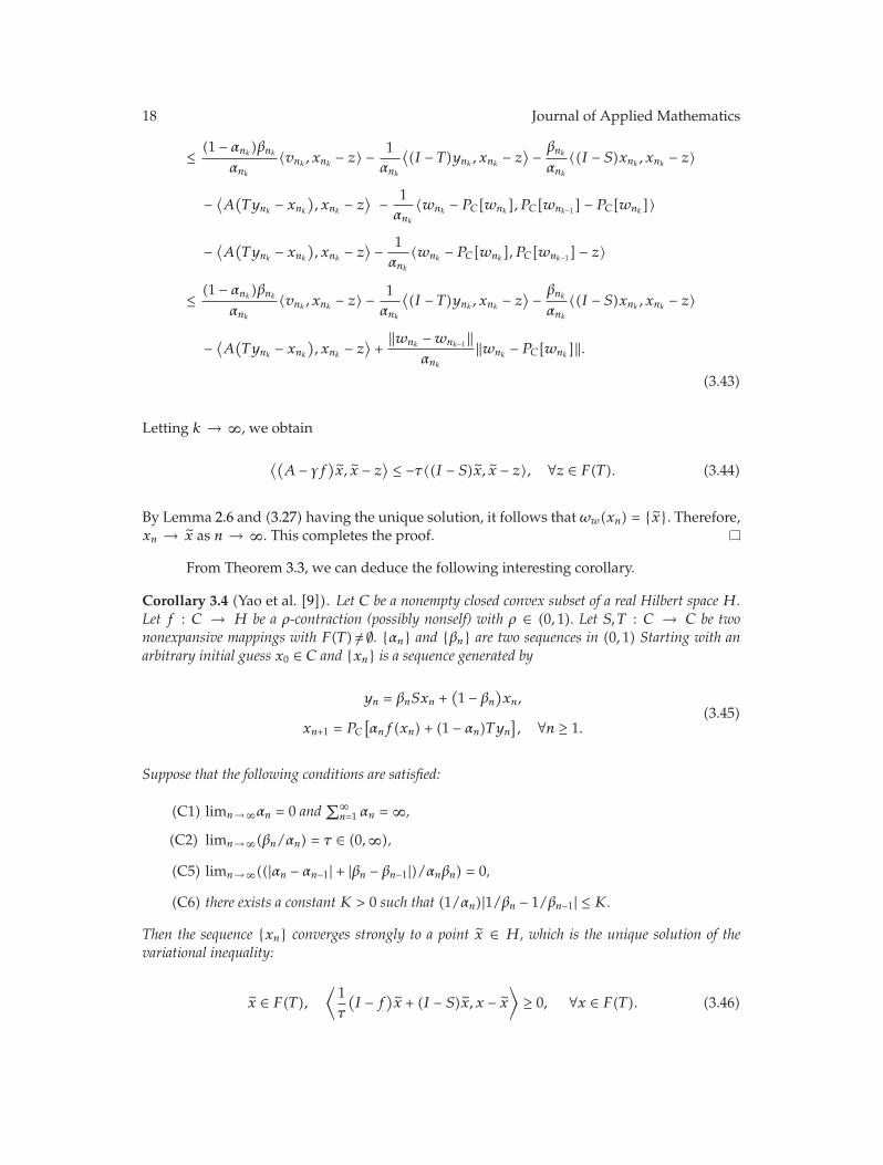
18 Journal of Applied Mathematics
≤ (1 − αnk)βnk
αnk
〈vnk , xnk − z〉 − 1αnk
⟨(I − T)ynk , xnk − z
⟩ − βnk
αnk
〈(I − S)xnk , xnk − z〉
− ⟨A(Tynk − xnk
), xnk − z
⟩ − 1αnk
〈wnk − PC[wnk], PC[wnk−1] − PC[wnk]〉
− ⟨A(Tynk − xnk
), xnk − z
⟩ − 1αnk
〈wnk − PC[wnk], PC[wnk−1] − z〉
≤ (1 − αnk)βnk
αnk
〈vnk , xnk − z〉 − 1αnk
⟨(I − T)ynk , xnk − z
⟩ − βnk
αnk
〈(I − S)xnk , xnk − z〉
− ⟨A(Tynk − xnk
), xnk − z
⟩+‖wnk −wnk−1‖
αnk
‖wnk − PC[wnk]‖.
(3.43)
Letting k → ∞, we obtain
⟨(A − γf
)x, x − z
⟩ ≤ −τ〈(I − S)x, x − z〉, ∀z ∈ F(T). (3.44)
By Lemma 2.6 and (3.27) having the unique solution, it follows that ωw(xn) = {x}. Therefore,xn → x as n → ∞. This completes the proof.
From Theorem 3.3, we can deduce the following interesting corollary.
Corollary 3.4 (Yao et al. [9]). Let C be a nonempty closed convex subset of a real Hilbert space H.Let f : C → H be a ρ-contraction (possibly nonself) with ρ ∈ (0, 1). Let S, T : C → C be twononexpansive mappings with F(T)/= ∅. {αn} and {βn} are two sequences in (0, 1) Starting with anarbitrary initial guess x0 ∈ C and {xn} is a sequence generated by
yn = βnSxn +(1 − βn
)xn,
xn+1 = PC
[αnf(xn) + (1 − αn)Tyn
], ∀n ≥ 1.
(3.45)
Suppose that the following conditions are satisfied:
(C1) limn→∞αn = 0 and∑∞
n=1 αn = ∞,
(C2) limn→∞(βn/αn) = τ ∈ (0,∞),
(C5) limn→∞((|αn − αn−1| + |βn − βn−1|)/αnβn) = 0,
(C6) there exists a constant K > 0 such that (1/αn)|1/βn − 1/βn−1| ≤ K.
Then the sequence {xn} converges strongly to a point x ∈ H, which is the unique solution of thevariational inequality:
x ∈ F(T),⟨
1τ
(I − f
)x + (I − S)x, x − x
⟩≥ 0, ∀x ∈ F(T). (3.46)

Journal of Applied Mathematics 19
Proof. As a matter of fact, if we take A = I and γ = 1 in Theorem 3.3 then this completes theproof.
Corollary 3.5 (Yao et al. [9]). Let C be a nonempty closed convex subset of a real Hilbert space H.Let S, T : C → C be two nonexpansive mappings with F(T)/= ∅. {αn} and {βn} are two sequences in(0, 1). Starting with an arbitrary initial guess x0 ∈ C and suppose {xn} is a sequence generated by
yn = βnSxn +(1 − βn
)xn,
xn+1 = PC
[(1 − αn)Tyn
], ∀n ≥ 1.
(3.47)
Suppose that the following conditions are satisfied:
(C1) limn→∞αn = 0 and∑∞
n=1 αn = ∞,
(C2) limn→∞(βn/αn) = 1,
(C5) limn→∞((|αn − αn−1| + |βn − βn−1|)/αnβn) = 0,
(C6) there exists a constant K > 0 such that (1/αn)|1/βn − 1/βn−1| ≤ K.
Then the sequence {xn} converges strongly to a point x ∈ H, which is the unique solution of thevariational inequality:
x ∈ F(T),⟨(
I − S
2
)x, x − x
⟩≥ 0, ∀x ∈ F(T). (3.48)
Proof . As a matter of fact, if we take A = I, f = 0, and γ = 1 in Theorem 3.3 then this iscompletes the proof.
Remark 3.6. Prototypes for the iterative parameters are, for example, αn = n−θ and βn = n−ω
(with θ,ω > 0). Since |αn − αn−1| ≈ n−θ and |βn − βn−1| ≈ n−ω, it is not difficult to prove that(C5) is satisfied for 0 < θ,ω < 1 and (C6) is satisfied if θ +ω ≤ 1.
Remark 3.7. Our results improve and extend the results of Yao et al. [9] by taking A = I andγ = 1 in Theorems 3.1 and 3.3.
The following is an example to support Theorem 3.3.
Example 3.8. Let H = R,C = [−1/4, 1/4], T = I, S = −I, A = I, f(x) = x2, PC = I, βn =
1/√n, αn = 1/
√n for every n ∈ N, we have τ = 1 and choose
−γ= 1/2, ρ = 1/3 and γ = 1. Then
{xn} is the sequence
xn+1 =x2n√n+(
1 − 1√n
)(1 − 2√
n
)xn, (3.49)
and xn → x = 0 as n → ∞, where x = 0 is the unique solution of the variational inequality
x ∈ F(T) =[−1
4,
14
],
⟨(3x − x2
), x − x
⟩≥ 0, ∀x ∈ F(T) =
[−1
4,
14
]. (3.50)

20 Journal of Applied Mathematics
Acknowledgments
The authors would like to thank the National Research University Project of Thailand’s Officeof the Higher Education Commission under the Project NRU-CSEC no. 55000613 for financialsupport.
References
[1] F. Deutsch and I. Yamada, “Minimizing certain convex functions over the intersection of the fixedpoint sets of nonexpansive mappings,” Numerical Functional Analysis and Optimization, vol. 19, no.1-2, pp. 33–56, 1998.
[2] I. Yamada, N. Ogura, Y. Yamashita, and K. Sakaniwa, “Quadratic optimization of fixed points ofnonexpansive mappings in Hilbert space,” Numerical Functional Analysis and Optimization, vol. 19, no.1-2, pp. 165–190, 1998.
[3] I. Yamada, “The hybrid steepest descent method for the variational inequality problem over theintersection of fixed point sets of nonexpansive mappings,” in Inherently Parallel Algorithms inFeasibility and Optimization and their Applications, D. Butnariu, Y. Censor, and S. Reich, Eds., pp. 473–504, Elsevier, 2001.
[4] H.-K. Xu, “Iterative algorithms for nonlinear operators,” Journal of the London Mathematical Society,vol. 66, no. 1, pp. 240–256, 2002.
[5] H. K. Xu, “An iterative approach to quadratic optimization,” Journal of Optimization Theory andApplications, vol. 116, no. 3, pp. 659–678, 2003.
[6] A. Moudafi, “Viscosity approximation methods for fixed-points problems,” Journal of MathematicalAnalysis and Applications, vol. 241, no. 1, pp. 46–55, 2000.
[7] H.-K. Xu, “Viscosity approximation methods for nonexpansive mappings,” Journal of MathematicalAnalysis and Applications, vol. 298, no. 1, pp. 279–291, 2004.
[8] G. Marino and H.-K. Xu, “A general iterative method for nonexpansive mappings in Hilbert spaces,”Journal of Mathematical Analysis and Applications, vol. 318, no. 1, pp. 43–52, 2006.
[9] Y. Yao, Y. J. Cho, and Y.-C. Liou, “Iterative algorithms for hierarchical fixed points problems andvariational inequalities,” Mathematical and Computer Modelling, vol. 52, no. 9-10, pp. 1697–1705, 2010.
[10] F. E. Browder, “Nonlinear operators and nonlinear equations of evolution in Banach spaces,” inProceedings of Symposia in Pure Mathematics, vol. 18, pp. 78–81, American Mathematical Society, 1976.
[11] G. L. Acedo and H.-K. Xu, “Iterative methods for strict pseudo-contractions in Hilbert spaces,”Nonlinear Analysis, vol. 67, no. 7, pp. 2258–2271, 2007.

Hindawi Publishing CorporationJournal of Applied MathematicsVolume 2012, Article ID 395760, 24 pagesdoi:10.1155/2012/395760
Research ArticleThe Modified Block Iterative Algorithms forAsymptotically Relatively NonexpansiveMappings and the System of Generalized MixedEquilibrium Problems
Kriengsak Wattanawitoon1 and Poom Kumam2
1 Department of Mathematics and Statistics, Faculty of Science and Agricultural Technology, RajamangalaUniversity of Technology Lanna Tak, Tak 63000, Thailand
2 Department of Mathematics, Faculty of Science, King Mongkut’s University of Technology Thonburi(KMUTT), Bangmod, Thrungkru, Bangkok 10140, Thailand
Correspondence should be addressed to Poom Kumam, [email protected]
Received 3 March 2012; Accepted 17 June 2012
Academic Editor: Hong-Kun Xu
Copyright q 2012 K. Wattanawitoon and P. Kumam. This is an open access article distributedunder the Creative Commons Attribution License, which permits unrestricted use, distribution,and reproduction in any medium, provided the original work is properly cited.
The propose of this paper is to present a modified block iterative algorithm for finding a commonelement between the set of solutions of the fixed points of two countable families of asymptoticallyrelatively nonexpansive mappings and the set of solution of the system of generalized mixedequilibrium problems in a uniformly smooth and uniformly convex Banach space. Our resultsextend many known recent results in the literature.
1. Introduction
The equilibrium problem theory provides a novel and unified treatment of a wide class ofproblems which arise in economics, finance, image reconstruction, ecology, transportation,networks, elasticity, and optimization, and it has been extended and generalized in manydirections.
In the theory of equilibrium problems, the development of an efficient and imple-mentable iterative algorithm is interesting and important. This theory combines theoreticaland algorithmic advances with novel domain of applications. Analysis of these problemsrequires a blend of techniques from convex analysis, functional analysis, and numericalanalysis.

2 Journal of Applied Mathematics
Let E be a Banach space with norm ‖ · ‖, C be a nonempty closed convex subset ofE, and let E∗ denote the dual of E. Let fi : C × C → R be a bifunction, ψi : C → R be areal-valued function, where R is denoted by the set of real numbers, and Ai : C → E∗ be anonlinear mapping. The goal of the system of generalized mixed equilibrium problem is to findu ∈ C such that
f1(u, y
)+⟨A1u, y − u
⟩+ ψ1
(y) − ψ1(u) ≥ 0, ∀y ∈ C,
f2(u, y
)+⟨A2u, y − u
⟩+ ψ2
(y) − ψ2(u) ≥ 0, ∀y ∈ C,
...
fN(u, y
)+⟨ANu, y − u
⟩+ ψN
(y) − ψN(u) ≥ 0, ∀y ∈ C.
(1.1)
If fi = f , Ai = A, and ψi = ψ, the problem (1.1) is reduced to the generalized mixed equilibriumproblem, denoted by GEMP(f,A, ψ), to find u ∈ C such that
f(u, y
)+⟨Au, y − u
⟩+ ψ
(y) − ψ(u) ≥ 0, ∀y ∈ C. (1.2)
The set of solutions to (1.2) is denoted by Ω, that is,
Ω ={x ∈ C : f
(u, y
)+⟨Au, y − u
⟩+ ϕ
(y) − ϕ(u) ≥ 0, ∀y ∈ C
}. (1.3)
If A = 0, the problem (1.2) is reduced to the mixed equilibrium problem for f , denoted byMEP(f, ψ), to find u ∈ C such that
f(u, y
)+ ψ
(y) − ψ(u) ≥ 0, ∀y ∈ C. (1.4)
If f ≡ 0, the problem (1.2) is reduced to the mixed variational inequality of Browder type,denoted by VI(C,A, ψ), is to find u ∈ C such that
⟨Au, y − u
⟩+ ψ
(y) − ψ(u) ≥ 0, ∀y ∈ C. (1.5)
If A = 0 and ψ = 0, the problem (1.2) is reduced to the equilibrium problem for f , denoted byEP(f), to find u ∈ C such that
f(u, y
) ≥ 0, ∀y ∈ C. (1.6)
The above formulation (1.6) was shown in [1] to cover monotone inclusion problems,saddle-point problems, variational inequality problems, minimization problems, vectorequilibrium problems, and Nash equilibria in noncooperative games. In addition, there areseveral other problems, for example, the complementarity problem, fixed-point problem, andoptimization problem, which can also be written in the form of an EP(f). In other words,the EP(f) is a unifying model for several problems arising in physics, engineering, science,economics, and so forth. In the last two decades, many papers have appeared in the literature

Journal of Applied Mathematics 3
on the existence of solutions to EP(f); see, for example [1–4] and references therein. Somesolution methods have been proposed to solve the EP(f); see, for example, [2, 4–15] andreferences therein. In 2005, Combettes and Hirstoaga [5] introduced an iterative scheme offinding the best approximation to the initial data when EP(f) is nonempty, and they alsoproved a strong convergence theorem.
A Banach space E is said to be strictly convex if ‖(x + y)/2‖ < 1 for all x, y ∈ E with‖x‖ = ‖y‖ = 1 and x /=y. Let U = {x ∈ E : ‖x‖ = 1} be the unit sphere of E. Then the Banachspace E is said to be smooth, provided
limt→ 0
∥∥x + ty
∥∥ − ‖x‖t
(1.7)
exists for each x, y ∈ U. It is also said to be uniformly smooth if the limit is attained uniformlyfor x, y ∈ E. The modulus of convexity of E is the function δ : [0, 2] → [0, 1] defined by
δ(ε) = inf{
1 −∥∥∥∥x + y
2
∥∥∥∥ : x, y ∈ E, ‖x‖ =∥∥y
∥∥ = 1,∥∥x − y
∥∥ ≥ ε
}. (1.8)
A Banach space E is uniformly convex, if and only if δ(ε) > 0 for all ε ∈ (0, 2].Let E be a Banach space, C be a closed convex subset of E, a mapping T : C → C is
said to be nonexpansive if
∥∥Tx − Ty∥∥ ≤ ∥∥x − y
∥∥ (1.9)
for all x, y ∈ C. We denote by F(T) the set of fixed points of T . If C is a bounded closedconvex set and T is a nonexpansive mapping of C into itself, then F(T) is nonempty (see[16]). A point p in C is said to be an asymptotic fixed point of T [17] if C contains a sequence{xn} which converges weakly to p such that limn→∞‖xn − Txn‖ = 0. The set of asymptoticfixed points of T will be denoted by F(T). A point p ∈ C is said to be a strong asymptotic fixedpoint of T , if there exists a sequence {xn} ⊂ C such that xn → p and ‖xn − Txn‖ → 0. Theset of strong asymptotic fixed points of T will be denoted by F(T). A mapping T from C intoitself is said to be relatively nonexpansive [18–20] if F(T) = F(T) and φ(p, Tx) ≤ φ(p, x) forall x ∈ C and p ∈ F(T). The asymptotic behavior of a relatively nonexpansive mapping wasstudied in [21, 22]. T is said to be φ-nonexpansive, if φ(Tx, Ty) ≤ φ(x, y) for x, y ∈ C. T issaid to be quas-φ-nonexpansive if F(T)/= ∅ and φ(p, Tx) ≤ φ(p, x) for x ∈ C and p ∈ F(T). Amapping T is said to be asymptotically relatively nonexpansive, if F(T)/= ∅, and there exists a realsequence {kn} ⊂ [1,∞) with kn → 1 such that φ(p, Tnx) ≤ knφ(p, x), for all n ≥ 1, x ∈ C, andp ∈ F(T). {Tn}∞n=0 is said to be a countable family of weak relatively nonexpansive mappings [23] ifthe following conditions are satisfied:
(i) F({Tn}∞n=0)/= ∅;
(ii) φ(u, Tnx) ≤ φ(u, x), for all u ∈ F(Tn), x ∈ C, n ≥ 0;
(iii) F({Tn}∞n=0) = ∩∞n=0F(Tn).

4 Journal of Applied Mathematics
A mapping T : C → C is said to be uniformly L-Lipschitz continuous, if there exists a constantL > 0 such that
∥∥Tnx − Tny
∥∥ ≤ L
∥∥x − y
∥∥, ∀x, y ∈ C, ∀n ≥ 1. (1.10)
A mapping T : C → C is said to be closed if for any sequence {xn} ⊂ C with xn → x andTxn → y, then Tx = y. Let {Ti}∞i=1 : C → C be a sequence of mappings. {Ti}∞i=1 is said to bea countable family of uniformly asymptotically relatively nonexpansive mappings, if ∩∞
n=1F(Tn)/= ∅,and there exists a sequence {kn} ⊂ [1,∞) with kn → 1 such that for each i > 1
φ(p, Tn
i x) ≤ knφ
(p, x
), ∀p ∈
∞⋂
n=1
F(Tn), x ∈ C, ∀n ≥ 1. (1.11)
In 2009, Petrot et al. [24], introduced a hybrid projection method for approximatinga common element of the set of solutions of fixed points of hemirelatively nonexpansive(or quasi-φ-nonexpansive) mappings in a uniformly convex and uniformly smooth Banachspace:
x0 ∈ C, C0 = C,
yn = J−1(αnJxn + (1 − αn)JTnzn),
zn = J−1(βnJxn +(1 − βn
)JTnxn
),
Cn+1 ={v ∈ Cn : φ
(v, yn
) ≤ φ(v, xn)},
xn+1 = ΠCn+1(x0).
(1.12)
They proved that the sequence {xn} converges strongly to p ∈ F(T), where p ∈ ΠF(T)x and ΠC
is the generalized projection from E onto F(T). Kumam and Wattanawitoon [25], introduceda hybrid iterative scheme for finding a common element of the set of common fixed points oftwo quasi-φ-nonexpansive mappings and the set of solutions of an equilibrium problem inBanach spaces, by the following manner:
x0 ∈ C, C0 = C
yn = J−1(αnJxn + (1 − αn)JSzn),
zn = J−1(βnJxn +(1 − βn
)JTxn
),
un ∈ C such that f(un, y
)+
1rn
⟨y − un, Jun − Jyn
⟩ ≥ 0, ∀y ∈ C,
Cn+1 ={z ∈ Cn : φ(z, un) ≤ φ(z, xn)
},
xn+1 = ΠCn+1(x0).
(1.13)

Journal of Applied Mathematics 5
They proved that the sequence {xn} converges strongly to p ∈ F(T) ∩ F(S) ∩ EP(f), wherep ∈ ΠF(T)∩F(S)∩EP(f)x under the assumptions (C1) lim supn→∞αn < 1, (C2) limn→∞βn < 1, and(C3) lim infn→∞(1 − αn)βn(1 − βn) > 0.
Recently, Chang et al. [26], introduced the modified block iterative method to proposean algorithm for solving the convex feasibility problems for an infinite family of quasi-φ-asymptotically nonexpansive mappings,
x0 ∈ C chosen arbitrary, C0 = C,
yn = J−1
(
αn,0Jxn +∞∑
i=1
αn,iJSni xn
)
,
Cn+1 ={v ∈ Cn : φ
(v, yn
) ≤ φ(v, xn) + ξn},
xn+1 = ΠCn+1x0, ∀n ≥ 0,
(1.14)
where ξn = supu∈F(kn − 1)φ(u, xn). Then, they proved that under appropriate controlconditions the sequence {xn} converges strongly to Π∩∞
n=1F(Si)x0.Very recently, Tan and Chang [27], introduced a new hybrid iterative scheme for
finding a common element between set of solutions for a system of generalized mixedequilibrium problems, set of common fixed points of a family of quasi-φ-asymptoticallynonexpansive mappings (which is more general than quasi-φ-nonexpansive mappings), andnull spaces of finite family of γ-inverse strongly monotone mappings in a 2-uniformly convexand uniformly smooth real Banach space.
In this paper, motivated and inspired by Petrot et al. [24], Kumam and Wattanawitoon[25], Chang et al. [26], and Tan and Chang [27], we introduce the new hybrid block algorithmfor two countable families of closed and uniformly Lipschitz continuous and uniformlyasymptotically relatively nonexpansive mappings in a Banach space. Let {xn} be a sequencedefined by x0 ∈ C, C0 = C and
yn = J−1
(
βn,0J(xn) +∞∑
i=1
βn,iJ(Tni xn
))
,
zn = J−1
(
αn,0J(xn) +∞∑
i=1
αn,iJ(Sni yn
))
,
u(i)n = Kfi,riKfi−1,ri−1 · · ·Kf1,r1(zn) , i = 1, 2, . . . ,N,
Cn+1 =
⎧⎨
⎩z ∈ Cn : max
i=1,2,...,Nφ(z, u
(i)n
)≤ φ(z, xn) + θn, φ
(z, yn
) ≤ φ(z, xn) + ξn
⎫⎬
⎭,
xn+1 = ΠCn+1x0, ∀n ≥ 0.
(1.15)
Under appropriate conditions, we will prove that the sequence {xn} generated by algorithms(1.15) converges strongly to the point Π(∩N
i=1Ωi)∩(∩∞i=1F(Ti))∩(∩∞
i=1F(Si))x0. Our results extend manyknown recent results in the literature.

6 Journal of Applied Mathematics
2. Preliminaries
Let E be a real Banach space with norm ‖ · ‖, and let J be the normalized duality mappingfrom E into 2E
∗given by
Jx = {x∗ ∈ E∗ : 〈x, x∗〉 = ‖x‖‖x∗‖, ‖x‖ = ‖x∗‖} (2.1)
for all x ∈ E, where E∗ denotes the dual space of E and 〈·, ·〉 the generalized duality pairingbetween E and E∗. It is also known that if E is uniformly smooth, then J is uniformly norm-to-norm continuous on each bounded subset of E.
We know the following (see [28, 29]):
(i) if E is smooth, then J is single valued;
(ii) if E is strictly convex, then J is one-to-one and 〈x − y, x∗ − y∗〉 > 0 holds for all(x, x∗), (y, y∗) ∈ J with x /=y;
(iii) if E is reflexive, then J is surjective;
(iv) if E is uniformly convex, then it is reflexive;
(v) if E is a reflexive and strictly convex, then J−1 is norm-weak-continuous;
(vi) E is uniformly smooth if and only if E∗ is uniformly convex;
(vii) if E∗ is uniformly convex, then J is uniformly norm-to-norm continuous on eachbounded subset of E;
(viii) each uniformly convex Banach space E has the Kadec-Klee property, that is, for anysequence {xn} ⊂ E, if xn ⇀ x ∈ E and ‖xn‖ → ‖x‖, then xn → x.
Let E be a smooth, strictly convex, and reflexive Banach space, and let C be a nonemptyclosed convex subset of E. Throughout this paper, we denote by φ the function defined by
φ(x, y
)= ‖x‖2 − 2
⟨x, Jy
⟩+∥∥y
∥∥2, for x, y ∈ E. (2.2)
Following Alber [30], the generalized projection ΠC : E → C is a map that assigns to anarbitrary point x ∈ E the minimum point of the function φ(x, y), that is, ΠCx = x, where x isthe solution to the minimization problem
φ(x, x) = infy∈C
φ(y, x
). (2.3)
Existence and uniqueness of the operator ΠC follows from the properties of the functionalφ(x, y) and strict monotonicity of the mapping J . It is obvious from the definition of functionφ that (see [30])
(∥∥y∥∥ − ‖x‖)2 ≤ φ
(y, x
) ≤ (∥∥y∥∥ + ‖x‖)2
, ∀x, y ∈ E. (2.4)
If E is a Hilbert space, then φ(x, y) = ‖x − y‖2.If E is a reflexive, strictly convex, and smooth Banach space, then for x, y ∈ E, φ(x, y) =
0 if and only if x = y. It is sufficient to show that if φ(x, y) = 0, then x = y. From (2.4), we

Journal of Applied Mathematics 7
have ‖x‖ = ‖y‖. This implies that 〈x, Jy〉 = ‖x‖2 = ‖Jy‖2. From the definition of J , one hasJx = Jy. Therefore, we have x = y; see [28, 29] for more details.
We also need the following lemmas for the proof of our main results.
Lemma 2.1 (see Kamimura and Takahashi [31]). Let E be a uniformly convex and smooth realBanach space, and let {xn}, {yn} be two sequences of E. If φ(xn, yn) → 0 and either {xn} or {yn} isbounded, then ‖xn − yn‖ → 0.
Lemma 2.2 (see Alber [30]). Let C be a nonempty closed convex subset of a smooth Banach space Eand x ∈ E. Then, x0 = ΠCx if and only if
⟨x0 − y, Jx − Jx0
⟩ ≥ 0, ∀y ∈ C. (2.5)
Lemma 2.3 (see Alber [30]). Let E be a reflexive, strictly convex, and smooth Banach space, let Cbe a nonempty closed convex subset of E, and let x ∈ E. Then
φ(y,ΠCx
)+ φ(ΠCx, x) ≤ φ
(y, x
), ∀y ∈ C. (2.6)
Lemma 2.4 (see Chang et al. [26]). Let E be a uniformly convex Banach space, r > 0 a positivenumber, and Br(0) a closed ball of E. Then, for any given sequence {xi}∞i=1 ⊂ Br(0) and for any givensequence {λi}∞i=1 of positive number with
∑∞n=1 λn = 1, there exists a continuous, strictly increasing,
and convex function g : [0, 2r) → [0,∞) with g(0) = 0 such that for any positive integers i, j withi < j,
∥∥∥∥∥
∞∑
n=1
λnxn
∥∥∥∥∥
2
≤∞∑
n=1
λn‖xn‖2 − λiλjg(∥∥xi − xj
∥∥). (2.7)
Lemma 2.5 (see Chang et al. [26]). Let E be a real uniformly smooth and strictly convex Banachspace with Kadec-Klee property, and C be a nonempty closed convex subset of E. Let T : C → C be aclosed and asymptotically relatively nonexpansive mapping with a sequence {kn} ⊂ [1,∞), kn → 1.Then F(T) is closed and convex subset of C.
For solving the generalized mixed equilibrium problem (or a system of generalizedmixed equilibrium problem), let us assume that the bifunction f : C×C → R and ψ : C → R
is convex and lower semicontinuous satisfies the following conditions:
(A1) f(x, x) = 0 for all x ∈ C;
(A2) f is monotone, that is, f(x, y) + f(y, x) ≤ 0 for all x, y ∈ C;
(A3) for each x, y, z ∈ C,
lim supt↓0
f(tz + (1 − t)x, y
) ≤ f(x, y
); (2.8)
(A4) for each x ∈ C, y �→ f(x, y) is convex and lower semicontinuous.

8 Journal of Applied Mathematics
Lemma 2.6 (see Chang et al. [26]). Let C be a closed convex subset of a smooth, strictly convex,and reflexive Banach space E. Let A : C → E∗ be a continuous and monotone mapping, ψ : C → R
is convex and lower semicontinuous and f be a bifunction from C × C to R satisfying (A1)–(A4). Forr > 0 and x ∈ E, then there exists u ∈ C such that
f(u, y
)+⟨Au, y − u
⟩+ ψ
(y) − ψ(u) +
1r
⟨y − u, Ju − Jx
⟩ ≥ 0, ∀y ∈ C. (2.9)
Define a mapping Kf,r : C → C as follows:
Kf,r(x) ={u ∈ C : f
(u, y
)+⟨Au, y − u
⟩+ ψ
(y) − ψ(u) +
1r
⟨y − u, Ju − Jx
⟩ ≥ 0, ∀y ∈ C
}
(2.10)
for all x ∈ E. Then, the following hold:
(i) Kf,r is singlevalued;
(ii) Kf,r is firmly nonexpansive, that is, for all x, y ∈ E, 〈Kf,rx −Kf,ry, JKf,rx − JKf,ry〉 ≤〈Kf,rx −Kf,ry, Jx − Jy〉;
(iii) F(Kf,r) = F(Kf,r);
(iv) u ∈ C is a solution of variational equation (2.9) if and only if u ∈ C is a fixed point ofKf,r ;
(v) F(Kf,r) = Ω;
(vi) Ω is closed and convex;
(vii) φ(p,Kf,rz) + φ(Kf,rz, z) ≤ φ(p, z), for all p ∈ F(Kf,r), z ∈ E.
3. Main Results
Theorem 3.1. Let E be a uniformly smooth and uniformly convex Banach space, let C be a nonempty,closed, and convex subset of E. Let Ai : C → E∗ be a continuous and monotone mapping,ψi : C → R be a lower semi-continuous and convex function, fi be a bifunction from C × C toR satisfying (A1)–(A4), Kfi,ri is the mapping defined by (2.10) where ri ≥ r > 0, and let {Ti}∞i=1,{Si}∞i=1 be countable families of closed and uniformly Li, μi-Lipschitz continuous and asymptoticallyrelatively nonexpansive mapping with sequence {kn}, {ζn} ⊂ [1,∞); kn → 1, ζn → 1 such that

Journal of Applied Mathematics 9
F := (∩Ni=1Ωi) ∩ (∩∞
i=1F(Ti)) ∩ (∩∞i=1F(Si))/= ∅. Let {xn} be a sequence generated by x0 ∈ C and
C0 = C,
yn = J−1
(
βn,0J(xn) +∞∑
i=1
βn,iJ(Tni xn
))
,
zn = J−1
(
αn,0J(xn) +∞∑
i=1
αn,iJ(Sni yn
))
,
u(i)n = Kfi,riKfi−1,ri−1 · · ·Kf1,r1(zn), i = 1, 2, . . . ,N,
Cn+1 ={z ∈ Cn : max
i=1,2,...,Nφ(z, u
(i)n
)≤ φ(z, xn) + θn, φ
(z, yn
) ≤ φ(z, xn) + ξn
},
xn+1 = ΠCn+1x0, ∀n ≥ 0,
(3.1)
where ξn = supp∈F(kn −1)φ(p, xn), θn = δn + ξnζn, and δn = supp∈F(ζn −1)φ(p, xn). The coefficientsequences {αn,i} and {βn,i} ⊂ [0, 1] satisfy the following:
(i)∑∞
i=0 αn,i = 1;
(ii)∑∞
i=0 βn,i = 1;
(iii) lim infn→∞αn,0αn,i > 0, for all i ≥ 1;
(iv) lim infn→∞βn,0βn,i > 0, for all i ≥ 1,
Ωi, i = 1, 2, . . . ,N is the set of solutions to the following generalized mixed equilibrium problem:
fi(z, y
)+⟨Aiz, y − z
⟩+ ψi
(y) − ψi(z) ≥ 0, ∀y ∈ C, i = 1, 2, . . . ,N. (3.2)
Then the sequence {xn} converges strongly toΠFx0.
Proof. We first show that Cn, for all n ≥ 0 is closed and convex. Clearly C0 = C is closed andconvex. Suppose that Ck is closed and convex for some k > 1. For each z ∈ Ck, we see thatφ(z, u(i)
k) ≤ φ(z, xk) is equivalent to
2(〈z, xk〉 −
⟨z, u
(i)k
⟩)≤ ‖xk‖2 −
∥∥∥u(i)k
∥∥∥2. (3.3)
By the set of Ck+1, we have
Cn+1 ={z ∈ Cn : max
i=1,2,...,Nφ(z, u
(i)n
)≤ φ(z, xn) + θn
}
=N⋂
i=1
{z ∈ C : φ
(z, u
(i)n
)≤ φ(z, xn) + θn
}.
(3.4)
Hence, Cn+1 is also closed and convex.

10 Journal of Applied Mathematics
By taking Θjn = Krj ,fiKrj−1,fj−1 · · ·Kr1,f1 for any j ∈ {1, 2, . . . , i} and Θ0
n = I for all n ≥ 1.
We note that u(i)n = Θi
nzn.Next, we show that F ⊂ Cn, for all n ≥ 1. For n ≥ 1, we have F ⊂ C = C1. For any given
p ∈ F := (∩Ni=1Ωi) ∩ (∩∞
i=1F(Ti)) ∩ (∩∞i=1F(Si)). By (3.1) and Lemma 2.4, we have
φ(p, yn
)= φ
(
p, J−1
( ∞∑
i=0
βn,iJTni xn
))
=∥∥p
∥∥2 −
∞∑
i=0
βn,i2⟨p, JTn
i xn
⟩+
∥∥∥∥∥
∞∑
i=0
βn,iJTni xn
∥∥∥∥∥
2
≤ ∥∥p
∥∥2 −
∞∑
i=0
βn,i2⟨p, JTn
i xn
⟩+
∞∑
i=0
βn,i∥∥JTn
i xn
∥∥2 − βn,0βn,ig
(∥∥JTn0 xn − JTn
i xn
∥∥)
=∥∥p
∥∥2 −∞∑
i=0
βn,i2⟨p, JTn
i xn
⟩+
∞∑
i=0
βn,i∥∥Tn
i xn
∥∥2 − βn,0βn,ig(∥∥Jxn − JTn
i xn
∥∥)
=∞∑
i=0
βn,iφ(p, Tn
i xn
) − βn,0βn,ig(∥∥Jxn − JTn
i xn
∥∥)
≤ knφ(p, xn
) − βn,0βn,ig(∥∥Jxn − JTn
i xn
∥∥)
≤ φ(p, xn
)+ sup
p∈F(kn − 1)φ
(p, xn
) − βn,0βn,ig(∥∥Jxn − JTn
i xn
∥∥)
≤ φ(p, xn
)+ ξn − βn,0βn,ig
(∥∥Jxn − JTni xn
∥∥)
≤ φ(p, xn
)+ ξn,
(3.5)
where ξn = supp∈F(kn − 1)φ(p, xn).By (3.1) and (3.5), we note that
φ(p, u
(i)n
)= φ
(p,Θi
nzn)
≤ φ(p, zn
)
≤ φ
(
p, J−1
(
αn,0Jxn +∞∑
i=1
JSni yn
))
=∥∥p
∥∥2 − 2
⟨
p, αn,0Jxn +∞∑
i=1
JSni yn
⟩
+
∥∥∥∥∥αn,0Jxn +
∞∑
i=1
JSni yn
∥∥∥∥∥
2
≤ ∥∥p∥∥2 − 2αn,0
⟨p, Jxn
⟩ − 2∞∑
i=1
αn,i
⟨p, JSn
i yn
⟩+ αn,0‖xn‖2 +
∞∑
i=1
∥∥Sni yn
∥∥2
− αn,0αn,ig∥∥Jxn − JSn
i yn
∥∥

Journal of Applied Mathematics 11
≤ αn,0φ(p, xn
)+
∞∑
i=1
αn,iφ(p, Sn
i yn
) − αn,0αn,ig∥∥Jxn − JSn
i yn
∥∥
≤ αn,0φ(p, xn
)+ ζn
∞∑
i=1
αn,iφ(p, yn
) − αn,0αn,ig∥∥Jxn − JSn
i yn
∥∥
≤ αn,0φ(p, xn
)+ ζn
∞∑
i=1
αn,i
(φ(p, xn
)+ ξn
) − αn,0αn,ig∥∥Jxn − JSn
i yn
∥∥
≤ αn,0φ(p, xn
)+ ζn
∞∑
i=1
αn,iφ(p, xn
)+ ξnζn
∞∑
i=1
αn,i − αn,0αn,ig∥∥Jxn − JSn
i yn
∥∥
≤ ζnφ(p, xn
)+ ξnζn
∞∑
i=1
αn,i − αn,0αn,ig∥∥Jxn − JSn
i yn
∥∥
≤ φ(p, xn
)+ sup
p∈F(ζn − 1)φ
(p, xn
)+ ξnζn
∞∑
i=1
αn,i − αn,0αn,ig∥∥Jxn − JSn
i yn
∥∥
≤ φ(p, xn
)+ δn + ξnζn − αn,0αn,ig
∥∥Jxn − JSni yn
∥∥
≤ φ(p, xn
)+ θn,
(3.6)
where δn = supp∈F(ζn − 1)φ(p, xn), θn = δn + ξnζn. By assumptions on {kn} and {ζn}, we have
ξn = supp∈F
(kn − 1)φ(p, xn
)
≤ supp∈F
(kn − 1)(∥∥p
∥∥ +M)2 −→ 0 as n −→ ∞,
(3.7)
δn = supp∈F
(ζn − 1)φ(p, xn
)
≤ supp∈F
(ζn − 1)(∥∥p
∥∥ +M)2 −→ 0 as n −→ ∞,
(3.8)
where M = supn≥0‖xn‖.So, we have p ∈ Cn+1. This implies that F ∈ Cn, for all n ≥ 0 and also {xn} is well
defined.From Lemma 2.2 and xn = ΠCnx0, we have
〈xn − z, Jx0 − Jxn〉 ≥ 0, ∀z ∈ Cn,
⟨xn − p, Jx0 − Jxn
⟩ ≥ 0, ∀p ∈ Cn.(3.9)
From Lemma 2.3, one has
φ(xn, x0) = φ(ΠCnx0, x0) ≤ φ(p, x0
) − φ(p, xn
) ≤ φ(p, x0
)(3.10)

12 Journal of Applied Mathematics
for all p ∈ F ⊂ Cn and n ≥ 1. Then, the sequence {φ(xn, x0)} is also bounded. Thus {xn} isbounded. Since xn = ΠCnx0 and xn+1 = ΠCn+1x0 ∈ Cn+1 ⊂ Cn, we have
φ(xn, x0) ≤ φ(xn+1, x0), ∀n ∈ N. (3.11)
Therefore, {φ(xn, x0)} is nondecreasing. Hence, the limit of {φ(xn, x0)} exists. By theconstruction of Cn, one has that Cm ⊂ Cn and xm = ΠCmx0 ∈ Cn for any positive integerm ≥ n. It follows that
φ(xm, xn) = φ(xm,ΠCnx0)
≤ φ(xm, x0) − φ(ΠCnx0, x0)
= φ(xm, x0) − φ(xn, x0).
(3.12)
Letting m,n → 0 in (3.12), we get φ(xm, xn) → 0. It follows from Lemma 2.1, that ‖xm −xn‖ → 0 as m,n → ∞. That is, {xn} is a Cauchy sequence.
Since {xn} is bounded and E is reflexive, there exists a subsequence {xni} ⊂ {xn} suchthat xni ⇀ u. Since Cn is closed and convex and Cn+1 ⊂ Cn, this implies that Cn is weaklyclosed and u ∈ Cn for each n ≥ 0. since xn = ΠCnx0, we have
φ(xni , x0) ≤ φ(u, x0), ∀ni ≥ 0. (3.13)
Since
lim infni →∞
φ(xni , x0) = lim infni →∞
{‖xni‖2 − 2〈xni , Jx0〉 + ‖x0‖2
}
≤ ‖u‖2 − 2〈u, Jx0〉 + ‖x0‖2
= φ(u, x0).
(3.14)
We have
φ(u, x0) ≤ lim infni →∞
φ(xni , x0) ≤ lim supni →∞
φ(xni , x0) ≤ φ(u, x0). (3.15)
This implies that limni →∞φ(xni , x0) = φ(u, x0). That is, ‖xni‖ → ‖u‖. Since xni ⇀ u, by theKadec-klee property of E, we obtain that
limn→∞
xni = u. (3.16)
If there exists some subsequence {xnj} ⊂ {xn} such that xnj → q, then we have
φ(u, q
)= lim
ni →∞,nj →∞φ(xni , xnj
)≤ lim
ni →∞,nj →∞
(φ(xni , x0) − φ
(ΠCnj
x0, x0
))
= limni →∞,nj →∞
(φ(xni , x0) − φ
(xnjx0, x0
))= 0.
(3.17)

Journal of Applied Mathematics 13
Therefore, we have u = q. This implies that
limn→∞
xn = u. (3.18)
Since
φ(xn+1, xn) = φ(xn+1,ΠCnx0) ≤ φ(xn+1, x0) − φ(ΠCnx0, x0)
= φ(xn+1, x0) − φ(xn, x0)(3.19)
for all n ∈ N, we also have
limn→∞
φ(xn+1, xn) = 0. (3.20)
Since xn+1 = ΠCn+1x0 ∈ Cn+1 and by the definition of Cn+1, for i = 1, 2, . . . ,N, we have
φ(xn+1, u
in
)≤ φ(xn+1, xn) + θn. (3.21)
Noticing that limn→∞φ(xn+1, xn) = 0, we obtain
limn→∞
φ(xn+1, u
in
)= 0, for i = 1, 2, . . . ,N. (3.22)
It then yields that limn→∞(‖xn+1‖−‖uin‖) = 0, for all i = 1, 2, . . . ,N. Since limn→∞‖xn+1‖ = ‖u‖,
we have
limn→∞
∥∥∥uin
∥∥∥ = ‖u‖, ∀i = 1, 2, . . . ,N. (3.23)
Hence,
limn→∞
∥∥∥Juin
∥∥∥ = ‖Ju‖, ∀i = 1, 2, . . . ,N. (3.24)
From Lemma 2.1 and (3.22), we have
limn→∞
‖xn+1 − xn‖ = limn→∞
∥∥∥xn+1 − uin
∥∥∥ = 0, ∀i = 1, 2, . . . ,N. (3.25)
By the triangle inequality, we get
limn→∞
∥∥∥xn − uin
∥∥∥ = 0, ∀i = 1, 2, . . . ,N. (3.26)
Since J is uniformly norm-to-norm continuous on bounded sets, we note that
limn→∞
∥∥∥Jxn − Juin
∥∥∥ = limn→∞
∥∥∥Jxn+1 − Juin
∥∥∥ = 0, ∀i = 1, 2, . . . ,N. (3.27)

14 Journal of Applied Mathematics
Now, we prove that u ∈ (∩∞i=1F(Ti)) ∩ (∩∞
i=1F(Si)). From the construction of Cn, weobtain that
φ(xn+1, yn
) ≤ φ(xn+1, xn) + ξn. (3.28)
From (3.7) and (3.20), we have
limn→∞
φ(xn+1, yn
)= 0. (3.29)
By Lemma 2.1, we also have
limn→∞
∥∥xn+1 − yn
∥∥ = 0. (3.30)
Since J is uniformly norm-to-norm continuous on bounded sets, we note that
limn→∞
∥∥Jxn+1 − Jyn
∥∥ = 0. (3.31)
From (2.4) and (3.29), we have (‖xn+1‖ − ‖yn‖)2 → 0. Since ‖xn+1‖ → ‖u‖, it yields that
∥∥yn
∥∥ −→ ‖u‖ as n −→ ∞. (3.32)
Since J is uniformly norm-to-norm continuous on bounded sets, it follows that
∥∥Jyn
∥∥ −→ ‖Ju‖ as n −→ ∞. (3.33)
This implies that {Jyn} is bounded in E∗. Since E is reflexive, there exists a subsequence{Jyni} ⊂ {Jyn} such that Jyni ⇀ r ∈ E∗. Since E is reflexive, we see that J(E) = E∗. Hence,there exists x ∈ E such that Jx = r. We note that
φ(xni+1, yni
)= ‖xni+1‖2 − 2
⟨xni+1, Jyni
⟩+∥∥yni
∥∥2
= ‖xni+1‖2 − 2⟨xni+1, Jyni
⟩+∥∥Jyni
∥∥2.
(3.34)
Taking the limit interior of both side and in view of weak lower semicontinuity of norm ‖ · ‖,we have
0 ≥ ‖u‖2 − 2〈u, r〉 + ‖r‖2
= ‖u‖2 − 2〈u, Jx〉 + ‖Jx‖2
= ‖u‖2 − 2〈u, Jx〉 + ‖x‖2 = φ(u, x),
(3.35)
that is, u = x. This implies that r = Ju and so Jyn ⇀ Jp. It follows from limn→∞‖Jyn‖ =‖Ju‖, as n → ∞ and the Kadec-Klee property of E∗ that Jyni → Ju as n → ∞. Note

Journal of Applied Mathematics 15
that J−1 : E∗ → E is hemicontinuous, it yields that yni ⇀ u. It follows from limn→∞‖un‖ =‖u‖, as n → ∞ and the Kadec-Klee property of E that limni →∞yni = u.
By similar, we can prove that
limn→∞
yn = u. (3.36)
By (3.20) and (3.30), we obtain
limn→∞
∥∥xn − yn
∥∥ = 0. (3.37)
Since J is uniformly norm-to-norm continuous on bounded sets, we note that
limn→∞
∥∥Jxn − Jyn
∥∥ = 0. (3.38)
So, from (3.27) and (3.31), by the triangle inequality, we get
limn→∞
∥∥∥Jyn − Juin
∥∥∥ = 0, for i = 1, 2, . . . ,N. (3.39)
Since J−1 is uniformly norm-to-norm continuous on bounded sets, we note that
limn→∞
∥∥∥yn − uin
∥∥∥ = 0, for i = 1, 2, . . . ,N. (3.40)
Since
φ(p, xn
) − φ(p, yn
)= ‖xn‖2 − ∥∥yn
∥∥2 − 2⟨p, Jxn − Jyn
⟩
≤ ‖xn‖2 − ∥∥yn
∥∥2 + 2∥∥p
∥∥∥∥Jxn − Jyn
∥∥
≤ ∥∥xn − yn
∥∥(‖xn‖ +∥∥yn
∥∥) + 2∥∥p
∥∥∥∥Jxn − Jyn
∥∥.
(3.41)
From (3.37) and (3.38), we obtain
φ(p, xn
) − φ(p, yn
) −→ 0, n −→ ∞. (3.42)
On the other hand, we observe that, for i = 1, 2, . . . ,N.
φ(p, xn
) − φ(p, ui
n
)= ‖xn‖2 −
∥∥∥uin
∥∥∥2 − 2
⟨p, Jxn − Jui
n
⟩
≤ ‖xn‖2 −∥∥∥ui
n
∥∥∥2+ 2
∥∥p∥∥∥∥∥Jxn − Jui
n
∥∥∥
≤∥∥∥xn − ui
n
∥∥∥(‖xn‖ +
∥∥∥uin
∥∥∥)+ 2
∥∥p∥∥∥∥∥Jxn − Jui
n
∥∥∥.
(3.43)

16 Journal of Applied Mathematics
From (3.22) and (3.27), we have
φ(p, xn
) − φ(p, ui
n
)−→ 0, n −→ ∞, ∀i = 1, 2, . . . ,N. (3.44)
For any p ∈ ∩Ni=1Ωi ∩ (∩∞
i=1F(Ti)) ∩ (∩∞i=1F(Si)), it follows from (3.5) that
βn,0βn,ig(∥∥Jxn − JTn
i xn
∥∥) ≤ φ
(p, xn
)+ ξn − φ
(p, yn
). (3.45)
From condition, lim infn→∞βn,0βn,i > 0, property of g, (3.7), and (3.42), we have that
∥∥Jxn − JTn
i xn
∥∥ −→ 0, n −→ ∞, ∀i = 1, 2, . . . ,N. (3.46)
Since xn → u and J is uniformly norm-to-norm continuous. It yields Jxn → Jp. Hence from(3.46), we have
∥∥xn − Tni xn
∥∥ −→ 0, n −→ ∞, ∀i = 1, 2, . . . ,N. (3.47)
Since xn → u, this implies that limn→∞JTni xn → Ju as n → ∞. Since J−1 : E∗ → E is
hemicontinuous, it follows that
Tni xn ⇀ u, for each i ≥ 1. (3.48)
On the other hand, for each i ≥ 1, we have
∥∥Tni xn
∥∥ − ‖u‖ =∣∣∥∥Tn
i xn
∥∥ − ‖u‖∣∣
≤ ∥∥Tni xn − u
∥∥ −→ 0, n −→ ∞.(3.49)
from this, together with (3.48) and the Kadec-Klee property of E, we obtain
Tni xn −→ u, for each i ≥ 1. (3.50)
On the other hand, by the assumption that Ti is uniformly Li-Lipschitz continuous, we have
∥∥∥Tn+1i xn − Tn
i xn
∥∥∥ ≤∥∥∥Tn+1
i xn − Tn+1i xn+1
∥∥∥ +∥∥∥Tn+1
i xn+1 − xn+1
∥∥∥
+ ‖xn+1 − xn‖ +∥∥xn − Tn
i xn
∥∥
≤ (Li + 1)‖xn+1 − xn‖ +∥∥∥Tn+1
i xn+1 − xn+1
∥∥∥
+∥∥xn − Tn
i xn
∥∥.
(3.51)

Journal of Applied Mathematics 17
By (3.18) and (3.50), we obtain
limn→∞
∥∥∥Tn+1
i xn − Tni xn
∥∥∥ = 0, ∀i ≥ 1, (3.52)
and limn→∞Tn+1i xn = u, that is, TiTnxn → u, for all i ≥ 1. By the closeness of Ti, we have
Tiu = u, for all i ≥ 1. This implies that u ∈ ∩∞i=1F(Ti).
By the similar way, we can prove that for each i ≥ 1
∥∥Jxn − JSn
i yn
∥∥ −→ 0, n −→ ∞. (3.53)
Since xn → u and J is uniformly norm-to-norm continuous. it yields Jxn → Jp. Hence from(3.53), we have
∥∥xn − Sni yn
∥∥ −→ 0, n −→ ∞. (3.54)
Since xn → u, this implies that limn→∞JSni yn → Ju as n → ∞. Since J−1 : E∗ → E is
hemicontinuous, it follows that
Sni yn ⇀ u, for each i ≥ 1. (3.55)
On the other hand, for each i ≥ 1, we have
∥∥Sni yn
∥∥ − ‖u‖ =∣∣∥∥Sn
i yn
∥∥ − ‖u‖∣∣
≤ ∥∥Sni yn − u
∥∥ −→ 0, n −→ ∞.(3.56)
From this, together with (3.54) and the Kadec-Klee property of E, we obtain
Sni yn −→ u, for each i ≥ 1. (3.57)
On the other hand, by the assumption that Si is uniformly μi-Lipschitz continuous, we have
∥∥∥Sn+1i yn − Sn
i yn
∥∥∥ ≤∥∥∥Sn+1
i yn − Sn+1i yn+1
∥∥∥ +∥∥∥Sn+1
i yn+1 − yn+1
∥∥∥
+∥∥yn+1 − yn
∥∥ +∥∥yn − Sn
i yn
∥∥
≤ (μi + 1
)∥∥yn+1 − yn
∥∥ +∥∥∥Sn+1
i yn+1 − yn+1
∥∥∥
+∥∥yn − Sn
i yn
∥∥.
(3.58)

18 Journal of Applied Mathematics
By (3.36) and (3.57), we obtain
limn→∞
∥∥∥Sn+1
i yn − Sni yn
∥∥∥ = 0 (3.59)
and limn→∞Sn+1i yn = u, that is, SiT
nyn → u. By the closeness of Si, we have Siu = u, for all i ≥1. This implies that u ∈ ∩∞
i=1F(Si). Hence u ∈ (∩∞i=1F(Ti)) ∩ (∩∞
i=1F(Si)).Next, we prove that u ∈ ∩N
i=1Ωi. For any p ∈ F, for each i = 1, 2, . . . ,N, we have
φ(uin, zn
)= φ
(Θi
nzn, zn)
≤ φ(p, zn
) − φ(p,Θi
nzn)
= φ(p, zn
) − φ(p, ui
n
)
≤ φ(p, xn
)+ θn − φ
(p, ui
n
)→ 0, as n → ∞.
(3.60)
It then yields that limn→∞(‖uin‖ − ‖zn‖) = 0. Since limn→∞‖ui
n‖ = ‖u‖, for all i ≥ 1, we have
limn→∞
‖zn‖ = ‖u‖. (3.61)
Hence,
limn→∞
‖Jzn‖ = ‖Ju‖. (3.62)
This together with limn→∞‖uin‖ = ‖u‖ show that for each i = 1, 2, . . . ,N,
limn→∞
∥∥∥uin − ui−1
n
∥∥∥ = limn→∞
∥∥∥Juin − Jui−1
n
∥∥∥ = 0, (3.63)
where u0n = zn. On the other hand, we have
uin = Kfi,riu
i−1n , for each i = 2, 3, . . . ,N, (3.64)
and uin is a solution of the following variational equation
fi(uin, y
)+⟨Aiu
in, y − ui
n
⟩+ ψi
(y) − ψi
(uin
)+
1ri
⟨y − ui
n, Juin − Jui−1
n
⟩≥ 0, ∀y ∈ C. (3.65)
By condition (A2), we note that
⟨Aiu
in, y − ui
n
⟩+ ψi
(y) − ψi
(uin
)+
1ri
⟨y − ui
n, Juin − Jui−1
n
⟩
≥ −fi(uin, y
)≥ fi
(y, ui
n
), ∀y ∈ C.
(3.66)

Journal of Applied Mathematics 19
By (A4), (3.63), and uin → u for each i = 2, 3, . . . ,N, we have
⟨Aiu, y − u
⟩+ ψi
(y) − ψi(u) ≥ fi
(y, u
), ∀y ∈ C. (3.67)
For 0 < t < 1 and y ∈ C, define yt = ty + (1 − t)u. Noticing that y, u ∈ C, we obtain yt ∈ C,which yields that
⟨Aiu, yt − u
⟩+ ψi
(yt
) − ψi(u) ≥ fi(yt, u
). (3.68)
In view of the convexity of φ it yields
t⟨Aiu, y − u
⟩+ t
(ψi
(y) − ψi(u)
) ≥ fi(yt, u
). (3.69)
It follows from (A1) and (A4) that
0 = fi(yt, yt
) ≤ tfi(yt, y
)+ (1 − t)fi
(yt, u
)
≤ tfi(yt, y
)+ (1 − t)t
[⟨Aiu, y − u
⟩+(ψi
(y) − ψi(u)
)].
(3.70)
Let t → 0, from (A3), we obtain the following:
fi(u, y
)+⟨Aiu, y − u
⟩+ ψi
(y) − ψi(u) ≥ 0, ∀y ∈ C, i = 1, 2, . . . ,N. (3.71)
This implies that u is a solution of the system of generalized mixed equilibrium problem (3.2),that is, u ∈ ∩N
i=1Ωi. Hence, u ∈ F := (∩Ni=1Ωi) ∩ (∩∞
i=1F(Ti)) ∩ (∩∞i=1F(Si)).
Finally, we show that xn → u = ΠFx0. Indeed from w ∈ F ⊂ Cn and xn = ΠCnx0, wehave the following:
φ(xn, x0) ≤ φ(w,x0), ∀n ≥ 0. (3.72)
This implies that
φ(u, x0) = limn→∞
φ(xn, x0) ≤ φ(w,x0). (3.73)
From the definition of ΠFx0 and (3.73), we see that u = w. This completes the proof.
Since every asymptotically relatively nonexpansive mappings is quasi-φ-nonexpan-sive mappings, hence we obtain the following corollary.
Corollary 3.2. Let E be a uniformly convex and uniformly smooth Banach space, let C be anonempty, closed, and convex subset of E. Let Ai : C → E∗ be a continuous and monotonemapping, ψi : C → R be a lower semi-continuous and convex function, fi be a bifunction fromC × C to R satisfying (A1)–(A4), Kfi,ri is the mapping defined by (2.10) where ri ≥ r > 0, andlet {Ti}∞i=1, {Si}∞i=1 be countable families of closed and quasi-φ-nonexpansive mapping such that
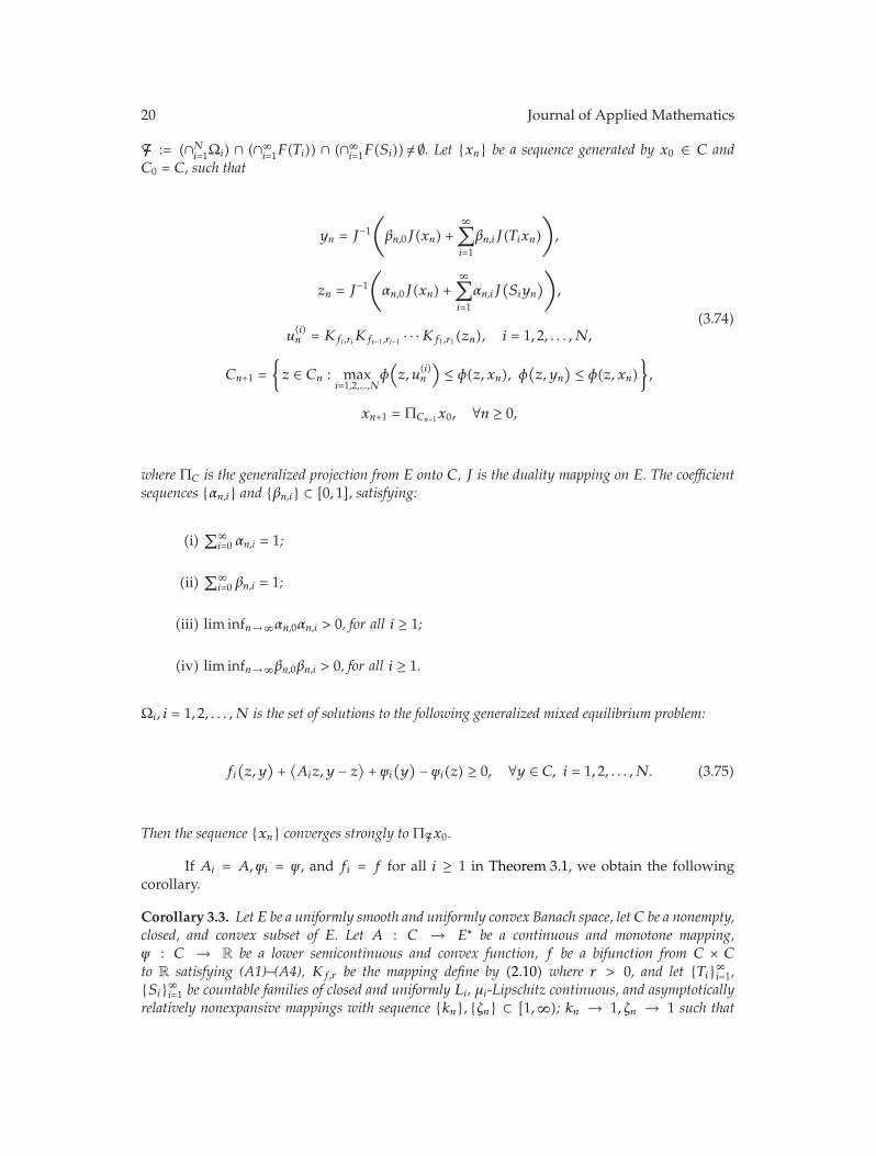
20 Journal of Applied Mathematics
F := (∩Ni=1Ωi) ∩ (∩∞
i=1F(Ti)) ∩ (∩∞i=1F(Si))/= ∅. Let {xn} be a sequence generated by x0 ∈ C and
C0 = C, such that
yn = J−1
(
βn,0J(xn) +∞∑
i=1
βn,iJ(Tixn)
)
,
zn = J−1
(
αn,0J(xn) +∞∑
i=1
αn,iJ(Siyn
))
,
u(i)n = Kfi,riKfi−1,ri−1 · · ·Kf1,r1(zn), i = 1, 2, . . . ,N,
Cn+1 ={z ∈ Cn : max
i=1,2,...,Nφ(z, u
(i)n
)≤ φ(z, xn), φ
(z, yn
) ≤ φ(z, xn)},
xn+1 = ΠCn+1x0, ∀n ≥ 0,
(3.74)
where ΠC is the generalized projection from E onto C, J is the duality mapping on E. The coefficientsequences {αn,i} and {βn,i} ⊂ [0, 1], satisfying:
(i)∑∞
i=0 αn,i = 1;
(ii)∑∞
i=0 βn,i = 1;
(iii) lim infn→∞αn,0αn,i > 0, for all i ≥ 1;
(iv) lim infn→∞βn,0βn,i > 0, for all i ≥ 1.
Ωi, i = 1, 2, . . . ,N is the set of solutions to the following generalized mixed equilibrium problem:
fi(z, y
)+⟨Aiz, y − z
⟩+ ψi
(y) − ψi(z) ≥ 0, ∀y ∈ C, i = 1, 2, . . . ,N. (3.75)
Then the sequence {xn} converges strongly toΠFx0.
If Ai = A,ψi = ψ, and fi = f for all i ≥ 1 in Theorem 3.1, we obtain the followingcorollary.
Corollary 3.3. Let E be a uniformly smooth and uniformly convex Banach space, letC be a nonempty,closed, and convex subset of E. Let A : C → E∗ be a continuous and monotone mapping,ψ : C → R be a lower semicontinuous and convex function, f be a bifunction from C × Cto R satisfying (A1)–(A4), Kf,r be the mapping define by (2.10) where r > 0, and let {Ti}∞i=1,{Si}∞i=1 be countable families of closed and uniformly Li, μi-Lipschitz continuous, and asymptoticallyrelatively nonexpansive mappings with sequence {kn}, {ζn} ⊂ [1,∞); kn → 1, ζn → 1 such that

Journal of Applied Mathematics 21
F := Ω ∩ (∩∞i=1F(Ti)) ∩ (∩∞
i=1F(Si))/= ∅. Let {xn} be a sequence generated by x0 ∈ C and C0 = C,such that
yn = J−1
(
βn,0J(xn) +∞∑
i=1
βn,iJ(Tni xn
))
,
zn = J−1
(
αn,0J(xn) +∞∑
i=1
αn,iJ(Sni yn
))
,
un = Kf,rzn,
Cn+1 ={z ∈ Cn : max
i=1,2,...,Nφ(z, u
(i)n
)≤ φ(z, xn) + θn, φ
(z, yn
) ≤ φ(z, xn) + ξn
},
xn+1 = ΠCn+1x0, ∀n ≥ 0,
(3.76)
where ξn = supp∈F(kn −1)φ(p, xn), θn = δn + ξnζn, and δn = supp∈F(ζn −1)φ(p, xn). The coefficientsequences {αn,i} and {βn,i} ⊂ [0, 1], satisfying:
(i)∑∞
i=0 αn,i = 1;
(ii)∑∞
i=0 βn,i = 1;
(iii) lim infn→∞αn,0αn,i > 0, for all i ≥ 1;
(iv) lim infn→∞βn,0βn,i > 0, for all i ≥ 1.
Then the sequence {xn} converges strongly toΠFx0.
If i = 1 in Theorem 3.1, then we obtain the following corollary.
Corollary 3.4. Let E be a uniformly smooth and uniformly convex Banach space, letC be a nonempty,closed, and convex subset of E. Let A : C → E∗ be a continuous and monotone mapping,ψ : C → R be a lower semicontinuous and convex function, f be a bifunction from C × C to R
satisfying (A1)–(A4), Kf,r is the mapping define by (2.10) where r > 0, and let T, S are two closedand uniformly L, μ-Lipschitz continuous and asymptotically relatively nonexpansive mappings withsequence {kn}, {ζn} ⊂ [1,∞); kn → 1, ζn → 1 such that F := Ω ∩ F(T) ∩ F(S)/= ∅. Let {xn} be asequence generated by x0 ∈ C and C0 = C, we have
yn = J−1(βnJxn +(1 − βn
)JTnxn
),
zn = J−1(αnJxn + (1 − αn)JSnyn
),
un = Kf,rzn,
Cn+1 ={z ∈ Cn : φ(z, un) ≤ φ(z, xn) + θn, φ
(z, yn
) ≤ φ(z, xn) + ξn},
xn+1 = ΠCn+1x0, ∀n ≥ 0,
(3.77)
where ξn = supp∈F(kn −1)φ(p, xn), θn = δn + ξnζn, and δn = supp∈F(ζn −1)φ(p, xn). The coefficientsequences {αn} and {βn} ⊂ [0, 1], satisfying

22 Journal of Applied Mathematics
(D1) lim infn→∞αn(1 − αn) > 0;
(D2) lim infn→∞βn(1 − βn) > 0.
Then the sequence {xn} converges strongly toΠFx0.
Remark 3.5. Theorem 3.1 and Corollary 3.3 improve and extend the corresponding results ofPetrot et al. [24], Kumam and Wattanawitoon [25], and Chang et al. [26] in the followingsenses:
(i) for the mappings, we extend the mappings from nonexpansive mappings, hemirel-atively nonexpansive mappings to two infinite family of closed asymptoticallyrelatively nonexpansive mappings;
(ii) from a solution of the classical equilibrium problem to a system of generalizedmixed equilibrium problems and the generalized mixed equilibrium problem withan infinite family of closed relatively nonexpansive mappings.
Remark 3.6. Corollary 3.4 improves and extends the corresponding results of Theorem 3.1 inKumam and Wattanawitoon [25] and Corollary 3.3 in Saewan et al. [11] in the followingsenses:
(i) the mapping in [11] and [25]
(ii) the conditions (D1) and (D2) of the parameters {αn} and {βn} are weaker andnot complicated than the conditions (C1)–(C3) in [[25], Theorem 3.1] and [[11],Theorem 3.1] which are easy to compute.
Acknowledgments
This first author was supported by The Hands-On Research and Development, RajamangalaUniversity of Technology Lanna (Grant no. UR2L003). Moreover, this work was supportedby the Higher Education Research Promotion and National Research University Project ofThailand, Office of the Higher Education Commission (NRU-CSEC Grant no. 55000613).
References
[1] E. Blum and W. Oettli, “From optimization and variational inequalities to equilibrium problems,” TheMathematics Student, vol. 63, no. 1–4, pp. 123–145, 1994.
[2] S. D. Flam and A. S. Antipin, “Equilibrium programming using proximal-like algorithms,” Mathemat-ical Programming, vol. 78, no. 1, pp. 29–41, 1997.
[3] A. Moudafi and M. Thera, “Proximal and dynamical approaches to equilibrium problems,” in Ill-Posed Variational Problems and Regularization Techniques, vol. 477 of Lecture Notes in Econom. and Math.Systems, pp. 187–201, Springer, Berlin, Germany, 1999.
[4] S. Takahashi and W. Takahashi, “Viscosity approximation methods for equilibrium problems andfixed point problems in Hilbert spaces,” Journal of Mathematical Analysis and Applications, vol. 331, no.1, pp. 506–515, 2007.
[5] P. L. Combettes and S. A. Hirstoaga, “Equilibrium programming in Hilbert spaces,” Journal of Nonlin-ear and Convex Analysis, vol. 6, no. 1, pp. 117–136, 2005.
[6] S. Saewan and P. Kumam, “Modified hybrid block iterative algorithm for convex feasibility problemsand generalized equilibrium problems for uniformly quasi-ϕ-asymptotically nonexpansive map-pings,” Abstract and Applied Analysis, vol. 2010, Article ID 357120, 22 pages, 2010.
[7] S. Saewan and P. Kumam, “A hybrid iterative scheme for a maximal monotone operator and twocountable families of relatively quasi-nonexpansive mappings for generalized mixed equilibrium and

Journal of Applied Mathematics 23
variational inequality problems,” Abstract and Applied Analysis, vol. 2010, Article ID 123027, 31 pages,2010.
[8] S. Saewan and P. Kumam, “The shrinking projection method for solving generalized equilibriumproblems and common fixed points for asymptotically quasi-ϕ-nonexpansive mappings,” Fixed PointTheory and Applications, vol. 2011, article 9, 2011.
[9] S. Saewan and P. Kumam, “Strong convergence theorems for countable families of uniformly quasi-ϕ-asymptotically nonexpansive mappings and a system of generalized mixed equilibrium problems,”Abstract and Applied Analysis, vol. 2011, Article ID 701675, 27 pages, 2011.
[10] S. Saewan and P. Kumam, “A modified hybrid projection method for solving generalized mixedequilibrium problems and fixed point problems in Banach spaces,” Computers & Mathematics withApplications, vol. 62, no. 4, pp. 1723–1735, 2011.
[11] S. Saewan, P. Kumam, and K. Wattanawitoon, “Convergence theorem based on a new hybrid pro-jection method for finding a common solution of generalized equilibrium and variational inequalityproblems in Banach spaces,” Abstract and Applied Analysis, vol. 2010, Article ID 734126, 25 pages, 2010.
[12] A. Tada and W. Takahashi, “Strong convergence theorem for an equilibrium problem and a non-expansive mapping,” in Nonlinear Analysis and Convex Analysis, pp. 609–617, Yokohama Publisher,Yokohama, Japan, 2006.
[13] A. Tada and W. Takahashi, “Weak and strong convergence theorems for a nonexpansive mapping andan equilibrium problem,” Journal of Optimization Theory and Applications, vol. 133, no. 3, pp. 359–370,2007.
[14] H. Zegeye and N. Shahzad, “Approximating common solution of variational inequality problems fortwo monotone mappings in Banach spaces,” Optimization Letters, vol. 5, no. 4, pp. 691–704, 2011.
[15] S. S. Zhang, C. K. Chan, and H. W. Joseph Lee, “Modified block iterative method for solving convexfeasibility problem, equilibrium problems and variational inequality problems,” Acta MathematicaSinica, vol. 28, no. 4, pp. 741–758, 2012.
[16] W. A. Kirk, “A fixed point theorem for mappings which do not increase distances,” The AmericanMathematical Monthly, vol. 72, pp. 1004–1006, 1965.
[17] S. Reich, “A weak convergence theorem for the alternating method with Bregman distances,” inTheory and Applications of Nonlinear Operators of Accretive and Monotone Type, vol. 178 of Lecture Notesin Pure and Applied Mathematics, pp. 313–318, Dekker, New York, NY, USA, 1996.
[18] W. Nilsrakoo and S. Saejung, “Strong convergence to common fixed points of countable relativelyquasi-nonexpansive mappings,” Fixed Point Theory and Applications, vol. 2008, Article ID 312454, 19pages, 2008.
[19] Y. Su, D. Wang, and M. Shang, “Strong convergence of monotone hybrid algorithm for hemi-relativelynonexpansive mappings,” Fixed Point Theory and Applications, vol. 2008, Article ID 284613, 8 pages,2008.
[20] H. Zegeye and N. Shahzad, “Strong convergence theorems for monotone mappings and relativelyweak nonexpansive mappings,” Nonlinear Analysis: Theory, Methods & Applications, vol. 70, no. 7, pp.2707–2716, 2009.
[21] D. Butnariu, S. Reich, and A. J. Zaslavski, “Asymptotic behavior of relatively nonexpansive operatorsin Banach spaces,” Journal of Applied Analysis, vol. 7, no. 2, pp. 151–174, 2001.
[22] Y. Censor and S. Reich, “Iterations of paracontractions and firmly nonexpansive operators withapplications to feasibility and optimization,” Optimization, vol. 37, no. 4, pp. 323–339, 1996.
[23] Y. Su, H.-k. Xu, and X. Zhang, “Strong convergence theorems for two countable families of weak rel-atively nonexpansive mappings and applications,” Nonlinear Analysis: Theory, Methods & Applications,vol. 73, no. 12, pp. 3890–3906, 2010.
[24] N. Petrot, K. Wattanawitoon, and P. Kumam, “Strong convergence theorems of modified Ishikawaiterations for countable hemi-relatively nonexpansive mappings in a Banach space,” Fixed Point The-ory and Applications, vol. 2009, Article ID 483497, 25 pages, 2009.
[25] P. Kumam and K. Wattanawitoon, “Convergence theorems of a hybrid algorithm for equilibriumproblems,” Nonlinear Analysis: Hybrid Systems, vol. 3, no. 4, pp. 386–394, 2009.
[26] S.-s. Chang, J. K. Kim, and X. R. Wang, “Modified block iterative algorithm for solving convex feasi-bility problems in Banach spaces,” Journal of Inequalities and Applications, vol. 2010, Article ID 869684,14 pages, 2010.
[27] J. F. Tan and S. S. Chang, “A new hybrid algorithm for solving a system of generalized mixed equi-librium problems, solving a family of quasi-ϕ-asymptotically nonexpansive mappings, and obtainingcommon fixed points in Banach space,” International Journal of Mathematics and Mathematical Sciences,vol. 2011, Article ID 106323, 16 pages, 2011.

24 Journal of Applied Mathematics
[28] I. Cioranescu, Geometry of Banach Spaces, Duality Mappings and Nonlinear Problems, vol. 62 of Mathemat-ics and Its Applications, Kluwer Academic Publishers, Dordrecht, The Netherlands, 1990.
[29] W. Takahashi, Nonlinear Functional Analysis, Yokohama Publishers, Yokohama, Japan, 2000, FixedPoint Theory and Its Applications.
[30] Y. I. Alber, “Metric and generalized projection operators in Banach spaces: properties and applica-tions,” in Theory and Applications of Nonlinear Operators of Accretive and Monotone Type, vol. 178 ofLecture Notes in Pure and Applied Mathematics, pp. 15–50, Dekker, New York, NY, USA, 1996.
[31] S. Kamimura and W. Takahashi, “Strong convergence of a proximal-type algorithm in a Banachspace,” SIAM Journal on Optimization, vol. 13, no. 3, pp. 938–945, 2002.

Hindawi Publishing CorporationJournal of Applied MathematicsVolume 2012, Article ID 629149, 13 pagesdoi:10.1155/2012/629149
Research ArticleOn Multivalued Nonexpansive Mappingsin R-Trees
K. Samanmit and B. Panyanak
Department of Mathematics, Faculty of Science, Chiang Mai University, Chiang Mai 50200, Thailand
Correspondence should be addressed to B. Panyanak, [email protected]
Received 25 April 2012; Accepted 20 June 2012
Academic Editor: Hong-Kun Xu
Copyright q 2012 K. Samanmit and B. Panyanak. This is an open access article distributed underthe Creative Commons Attribution License, which permits unrestricted use, distribution, andreproduction in any medium, provided the original work is properly cited.
The relationships between nonexpansive, weakly nonexpansive, ∗-nonexpansive, proximally non-expansive, proximally continuous, almost lower semicontinuous, and ε-semicontinuous mappingsin R-trees are studied. Convergence theorems for the Ishikawa iteration processes are also dis-cussed.
1. Introduction
A mapping t on a subset E of a Banach space (X, ‖ · ‖) is said to be nonexpansive if
∥∥t(x) − t(y)∥∥ ≤ ∥∥x − y
∥∥, ∀x, y ∈ E. (1.1)
A point x in E is called a fixed point of t if x = t(x). The existence of fixed points for non-expansive mappings in Banach spaces was studied independently by three authors in 1965(see Browder [1], Gohde [2], and Kirk [3]). They showed that every nonexpansive mappingdefined on a bounded closed convex subset of a uniformly convex Banach space always has afixed point. Since then many researchers generalized the concept of nonexpansive mappingsin different directions and also studied the fixed point theory for various types of generalizednonexpansive mappings.
Browder-Gohde-Kirk’s result was extended to multivalued nonexpansive mappingsby Lim [4] in 1974. Husain and Tarafdar [5] and Husain and Latif [6] introduced the con-cepts of weakly nonexpansive and ∗-nonexpansive multivalued mappings and studied theexistence of fixed points for such mappings in uniformly convex Banach spaces. In 1991, Xu[7] pointed out that a weakly nonexpansive multivalued mapping must be nonexpansiveand thus the main results of Husain-Tarafdar and Husain-Latif on weakly nonexpansive

2 Journal of Applied Mathematics
multivalued mappings are special cases of those of Lim [4]. Xu [7] also showed that ∗-non-expansiveness is different from nonexpansiveness for multivalued mappings. In 1995, LopezAcedo and Xu [8] introduced the concept of proximally nonexpansive multivalued mappingsand proved that it coincides with the concept of ∗-nonexpansive mappings when the map-pings take compact values.
In 2009, Shahzad and Zegeye [9] proved strong convergence theorems of the Ishikawaiteration for quasi-nonexpansive multivalued mappings satisfying the endpoint condition.They also constructed a modified Ishikawa iteration for proximally nonexpansive mappingsand proved strong convergence theorems of the proposed iteration without the endpointcondition. Puttasontiphot [10] gave the analogous results of Shahzad and Zegeye in completeCAT(0) spaces. However, there is not any result in linear or nonlinear spaces concerningthe convergence of Ishikawa iteration for quasi-nonexpansive multivalued mappings whichcompletely removes the endpoint condition.
In this paper, motivated by the above results, we obtain the relationships between non-expansive, weakly nonexpansive, ∗-nonexpansive, and proximally nonexpansive mappingsin a nice subclass of CAT(0) spaces, namely, R-trees. We also introduce a condition on map-pings which is much more general than the endpoint condition and prove strong convergencetheorems of a modified Ishikawa iteration for quasi-nonexpansive multivalued mappingssatisfying such condition.
2. Preliminaries
Let (X, d) be a metric space and let ∅/=E ⊆ X, x ∈ X. The distance from x to E is defined by
dist(x, E) = inf{d(x, y
): y ∈ E
}. (2.1)
The set E is called proximal if for each x ∈ X, there exists an element y ∈ E such that d(x, y) =dist(x, E). Let ε > 0 and x0 ∈ X. We will denote the open ball centered at x0 with radius εby B(x0, ε), the closed ε-hull of E by Nε(E) = {x ∈ X : dist(x, E) ≤ ε}, and the family ofnonempty subsets of E by 2E. Let H(·, ·) be the Hausdorff distance on 2E, that is,
H(A,B) = max
{
supa∈A
dist(a, B), supb∈B
dist(b,A)
}
, A, B ∈ 2E. (2.2)
Let T : E → 2E be a multivalued mapping. For each x ∈ E, we let
PT(x)(x) := {u ∈ T(x) : d(x, u) = dist(x, T(x))}. (2.3)
In the case of PT(x)(x) is a singleton; we will assume, without loss of generality, that PT(x)(x)is a point in E. A point x ∈ E is called a fixed point of T if x ∈ T(x). A point x ∈ E is called anendpoint of T if x is a fixed point of T and T(x) = {x}. We will denote by Fix(T) the set of allfixed points of T and by End(T) the set of all endpoints of T . We see that for each mappingT , End(T) ⊆ Fix(T) and the converse is not true in general. A mapping T is said to satisfy theendpoint condition if End(T) = Fix(T).

Journal of Applied Mathematics 3
Definition 2.1. Let E be a nonempty subset of a metric space (X, d) and T : E → 2E. Then T issaid to be
(i) nonexpansive if H(T(x), T(y)) ≤ d(x, y) for all x, y ∈ E;
(ii) quasi-nonexpansive if Fix(T)/= ∅ and
H(T(x), T
(p)) ≤ d
(x, p
) ∀x ∈ E, p ∈ Fix(T); (2.4)
(iii) weakly nonexpansive if for each x, y ∈ E and ux ∈ T(x), there exists uy ∈ T(y) suchthat
d(ux, uy
) ≤ d(x, y
); (2.5)
(iv) ∗-nonexpansive if for each x, y ∈ E and ux ∈ PT(x)(x), there exists uy ∈ PT(y)(y) suchthat
d(ux, uy
) ≤ d(x, y
); (2.6)
(v) proximally nonexpansive if the map F : E → 2E defined by F(x) := PT(x)(x) is non-expansive;
(vi) proximally continuous if the map F(x) := PT(x)(x) is continuous;
(vii) almost lower semicontinuous if given ε > 0, for each x ∈ E there is an open neighbor-hood U of x such that
⋂
y∈UNε
(T(y))
/= ∅; (2.7)
(viii) ε-semicontinuous if given ε > 0, for each x ∈ E there is an open neighborhood U of xsuch that
T(y) ∩Nε(T(x))/= ∅ ∀y ∈ U. (2.8)
The following facts can be found in [7, 8].
Proposition 2.2. Let E be a nonempty subset of a metric space (X, d) and T : E → 2E be a multi-valued mapping. Then the following statements hold:
(i) if T is weakly nonexpansive, then T is nonexpansive;
(ii) if T is ∗-nonexpansive and T takes nonempty proximal values, then T is proximally non-expansive;
(iii) the converses of (i) and (ii) hold if T takes compact values.

4 Journal of Applied Mathematics
For any pair of points x, y in a metric space (X, d), a geodesic path joining these pointsis an isometry c from a closed interval [0, l] to X such that c(0) = x and c(l) = y. The image ofc is called a geodesic segment joining x and y. If there exists exactly one geodesic joining x andy we denote by [x, y] the geodesic joining x and y. For x, y ∈ X and α ∈ [0, 1], we denote thepoint z ∈ [x, y] such that d(x, z) = αd(x, y) by (1 − α)x ⊕ αy. The space (X, d) is said to be ageodesic space if every two points of X are joined by a geodesic, and X is said to be uniquelygeodesic if there is exactly one geodesic joining x and y for each x, y ∈ X. A subset E of X issaid to be convex if E includes every geodesic segment joining any two of its points, and E issaid to be gated if for any point x /∈ E there is a unique point yx such that for any z ∈ E,
d(x, z) = d(x, yx
)+ d
(yx, z
). (2.9)
The point yx is called the gate of x in E. From the definition of yx we see that it is also theunique nearest point of x in E. The set E is called geodesically bounded if there is no geodesicray in E, that is, an isometric image of [0,∞). We will denote by P(E) the family of nonemptyproximinal subsets of E, by CC(E) the family of nonempty closed convex subsets of E, andby KC(E) the family of nonempty compact convex subsets of E.
Definition 2.3. An R-tree (sometimes called metric tree) is a geodesic metric space X such that:
(i) there is a unique geodesic segment [x, y] joining each pair of points x, y ∈ X;
(ii) if [y, x] ∩ [x, z] = {x}, then [y, x] ∪ [x, z] = [y, z].
By (i) and (ii) we have
(i) if u, v,w ∈ X, then [u, v] ∩ [u,w] = [u, z] for some z ∈ X.
An R-tree is a special case of a CAT(0) space. For a thorough discussion of these spacesand their applications, see [11]. Notice also that a metric space X is a complete R-tree if andonly if X is hyperconvex with unique metric segments, see [12]. For more about hyperconvexspaces and fixed point theorems in hyperconvex spaces, see [13]. We now collect some basicproperties of R-trees.
Lemma 2.4. Let X be a complete R-tree. Then the following statements hold:
(i) [14, page 1048] the gate subsets of X are precisely its closed and convex subsets;
(ii) [11, page 176] if E is a closed convex subset ofX, then, for each x ∈ X, there exists a uniquepoint PE(x) ∈ E such that
d(x, PE(x)) = dist(x, E); (2.10)
(iii) [11, page 176] if E is closed convex and if x′ belong to [x, PE(x)], then PE(x′) = PE(x);
(iv) [15, Lemma 3.1] if A and B are closed convex subsets of X, then, for any u ∈ X,
d(PA(u), PB(u)) ≤ H(A,B); (2.11)

Journal of Applied Mathematics 5
(v) [16, Lemma 3.2] if E is closed convex, then, for any x, y ∈ X, one has either
PE(x) = PE
(y)
(2.12)
or
d(x, y
)= d(x, PE(x)) + d
(PE(x), PE
(y))
+ d(PE
(y), y
); (2.13)
(vi) [17, Lemma 2.5] if x, y, z ∈ X and α ∈ [0, 1], then
d2((1 − α)x ⊕ αy, z) ≤ (1 − α)d2(x, z) + αd2(y, z
) − α(1 − α)d2(x, y); (2.14)
(vii) [18, Proposition 1] if E is a closed convex subset of X and T : E → CC(E) is a quasi-non-expansive mapping, then Fix(T) is closed and convex.
3. Results in R-Trees
In general metric spaces, the concepts of nonexpansive and ∗-nonexpansive multivaluedmappings are different (see Examples 5.1 and 5.2). But, if we restrict ourself to an R-tree wecan show that every nonexpansive mapping with nonempty closed convex values is a ∗-non-expansive mapping. The following lemma is very crucial.
Lemma 3.1. Let E be a nonempty closed convex subset of a complete R-tree X and v /∈ E. If v ∈[PE(v), u] for some u ∈ X, then PE(v) = PE(u).
Proof. By Lemma 2.4(iii), PE(x) = PE(v) for all x ∈ [PE(v), v]. Then for z ∈ E, we have
d(z, x) = d(z, PE(v)) + d(PE(v), x) ∀x ∈ [PE(v), v]. (3.1)
This implies that PE(v) is the gate of z in [PE(v), v] for all z ∈ E. Since v ∈ [PE(v), u], then vis the gate of u in [PE(v), v]. By Lemma 2.4(v), for each z ∈ E we have
d(u, z) = d(u, v) + d(v, PE(v)) + d(PE(v), z)
= d(u, PE(v)) + d(PE(v), z)
≥ d(u, PE(v)).
(3.2)
Hence PE(v) = PE(u) as desired.
Proposition 3.2. Let E be a nonempty subset of a complete R-tree X and T : E → 2E be a multi-valued mapping. If T takes closed and convex values, then the following statements hold:
(i) T is weakly nonexpansive if and only if T is nonexpansive;
(ii) T is ∗-nonexpansive if and only if T is proximally nonexpansive;
(iii) if T is nonexpansive, then T is proximally nonexpansive;

6 Journal of Applied Mathematics
(iv) if T is proximally nonexpansive, then T is proximally continuous;
(v) if T is proximally continuous, then T is almost lower semicontinuous;
(vi) if T is almost lower semicontinuous, then T is ε-semicontinuous.
Proof. (i) (⇒) Follows from Proposition 2.2(i). (⇐): let x, y ∈ E and ux ∈ T(x). Choose uy =PT(y)(ux). Then
d(ux, uy
)= dist
(ux, T
(y))
≤ H(T(x), T
(y))
≤ d(x, y
).
(3.3)
(ii) (⇒) Follows from Proposition 2.2(ii). (⇐): for each x ∈ E, we let ux = PT(x)(x).Then
d(ux, uy
)= d
(PT(x)(x), PT(y)
(y)) ≤ d
(x, y
). (3.4)
This means T is ∗-nonexpansive.(iii) We let x, y ∈ E and divide the proof to 3 cases.Case 1. PT(x)(x), PT(y)(y) ∈ [x, y]. Then d(PT(x)(x), PT(y)(y)) ≤ d(x, y).Case 2. PT(x)(x) /∈ [x, y], PT(y)(y) ∈ [x, y] or vice versa. Let u ∈ [PT(y)(y), y]. Then by
Lemma 2.4(iii), PT(y)(y) = PT(y)(u). We claim that PT(x)(x) = PT(x)(u). Let v be the gate ofPT(x)(x) in [x, y]. Then v /=PT(x)(x). Since v ∈ [x, PT(x)(x)], then by Lemma 2.4(iii) we havePT(x)(v) = PT(x)(x). This implies that v ∈ [PT(x)(v), u]. Since v /∈ T(x), by Lemma 3.1 we have
PT(x)(x) = PT(x)(v) = PT(x)(u). (3.5)
By Lemma 2.4(iv),
d(PT(x)(x), PT(y)
(y))
= d(PT(x)(u), PT(y)(u)
)
≤ H(T(x), T
(y))
≤ d(x, y
).
(3.6)
Case 3. PT(x)(x) /∈ [x, y] and PT(y)(y) /∈ [x, y]. Let v and w be the gates of PT(x)(x) andPT(y)(y) in [x, y], respectively. Since v ∈ [PT(x)(x), x] and w ∈ [PT(y)(y), y], then
PT(x)(x) = PT(x)(v), PT(y)(y)= PT(y)(w). (3.7)
Let u ∈ [v,w]. Then by Lemma 3.1, we have
PT(x)(v) = PT(x)(u), PT(y)(w) = PT(y)(u). (3.8)

Journal of Applied Mathematics 7
By (3.7), we have
PT(x)(x) = PT(x)(u), PT(y)(y)= PT(y)(u). (3.9)
By Lemma 2.4(iv),
d(PT(x)(x), PT(y)
(y))
= d(PT(x)(u), PT(y)(u)
)
≤ H(T(x), T
(y))
≤ d(x, y
).
(3.10)
(iv) Follows from the fact that nonexpansiveness implies continuity.(v) Given ε > 0 and let x0 ∈ E. Since the map F(x) = PT(x)(x) is single valued contin-
uous, then there exists δ > 0 such that
d(PT(x)(x), PT(x0)(x0)
)< ε ∀x ∈ B(x0, δ). (3.11)
Let U = B(x0, δ). Then U is an open neighborhood of x0. Since
dist(PT(x0)(x0), T(x)
) ≤ d(PT(x0)(x0), PT(x)(x)
)< ε ∀x ∈ U, (3.12)
then
PT(x0)(x0) ∈⋂
x∈UNε(T(x)). (3.13)
Therefore, T is almost lower semicontinuous.(vi) See [19, page 114].
The following result can be found in [19, Theorem 4].
Proposition 3.3. LetX be a completeR-tree,E a nonempty closed convex geodesically bounded subsetof X, and T : E → CC(E) an ε-semicontinuous mapping. Then T has a fixed point.
As a consequence of Propositions 3.2 and 3.3, we obtain the following.
Corollary 3.4. Let E be a nonempty closed convex geodesically bounded subset of a complete R-treeX and T : E → CC(E) be a multivalued mapping. Then T has a fixed point if one of the followingstatements holds:
(i) T is weakly nonexpansive;
(ii) T is nonexpansive;
(iii) T is ∗-nonexpansive;(iv) T is proximally nonexpansive;
(v) T is proximally continuous;
(vi) T is almost lower semicontinuous.

8 Journal of Applied Mathematics
4. Convergence Theorems
Let E be a nonempty convex subset of an R-tree X,T : E → P(E) a multivalued mapping and{αn},{βn} ⊆ [0, 1].
(A) The sequence of Ishikawa iterates [9] is defined by x1 ∈ E,
yn = βnzn ⊕(1 − β
)xn, n ≥ 1, (4.1)
where zn ∈ PT(xn)(xn), and
xn+1 = αnz′n ⊕ (1 − αn)xn, n ≥ 1, (4.2)
where z′n ∈ PT(yn)(yn).Recall that a multivalued mapping T : E → P(E) is said to satisfy Condition (I) if there
is a nondecreasing function f : [0,∞) → [0,∞) with f(0) = 0, f(r) > 0 for r ∈ (0,∞) suchthat
dist(x, T(x)) ≥ f(dist(x,Fix(T))) ∀x ∈ E. (4.3)
The mapping T is called hemicompact if for any sequence {xn} in E such that
limn→∞
dist(xn, T(xn)) = 0, (4.4)
there exists a subsequence {xnk} of {xn} and q ∈ E such that limk→∞xnk = q.The following theorems are consequences of [10, Theorems 3.6 and 3.7].
Theorem 4.1. Let X be a complete R-tree, E a nonempty closed convex subset of X, and T : E →P(E) a proximally nonexpansive mapping with Fix(T)/= ∅. Let {xn} be the Ishikawa iterates definedby (A). Assume that T satisfies condition (I) and αn, βn ∈ [a, b] ⊂ (0, 1). Then {xn} converges to afixed point of T .
Theorem 4.2. Let X be a complete R-tree, E a nonempty closed convex subset of X, and T : E →P(E) a proximally nonexpansive mapping with Fix(T)/= ∅. Let {xn} be the Ishikawa iterates definedby (A). Assume that T is hemicompact and (i) 0 ≤ αn, βn < 1; (ii) βn → 0; (iii)
∑αnβn = ∞. Then
{xn} converges to a fixed point of T .
As consequences of Proposition 3.2, Theorems 4.1 and 4.2, we obtain the following.
Corollary 4.3. Let X be a complete R-tree, E a nonempty closed convex subset of X, and T : E →CC(E) a nonexpansive mapping with Fix(T)/= ∅. Let {xn} be the Ishikawa iterates defined by (A).Assume that T satisfies condition (I) and αn, βn ∈ [a, b] ⊂ (0, 1). Then {xn} converges to a fixed pointof T .
Corollary 4.4. Let X be a complete R-tree, E a nonempty closed convex subset of X, and T : E →CC(E) a nonexpansive mapping with Fix(T)/= ∅. Let {xn} be the Ishikawa iterates defined by (A).Assume that T is hemicompact and (i) 0 ≤ αn, βn < 1; (ii) βn → 0 and (iii)
∑αnβn = ∞. Then {xn}
converges to a fixed point of T .

Journal of Applied Mathematics 9
Definition 4.5. Let E be a nonempty subset of a complete R-tree and T : E → CC(E) bea multivalued mapping for which Fix(T)/= ∅. We say that u ∈ E is a key of T if, for eachx ∈ Fix(T), x is the gate of u in T(x). We say that T satisfies the gate condition if T has a key inE.
It follows from the definitions that the endpoint condition implies the gate conditionand the converse is not true. Example 5.3 shows that there is a nonexpansive mapping satis-fying the gate condition but does not satisfy the endpoint condition.
Motivated by the above results, we introduce a modified Ishikawa iteration as follows:let E be a nonempty convex subset of an R-tree X, T : E → CC(E) a multivalued mapping,and {αn}, {βn} ⊆ [0, 1]. Fix u ∈ E.
(B) The sequence of Ishikawa iterates is defined by x1 ∈ E,
yn = βnzn ⊕(1 − βn
)xn, n ≥ 1, (4.5)
where zn is the gate of u in T(xn), and
xn+1 = αnz′n ⊕ (1 − αn)xn, n ≥ 1, (4.6)
where z′n is the gate of u in T(yn).Recall that a sequence {xn} in a metric space (X, d) is said to be Fejer monotone with
respect to a subset E of X if
d(xn+1, p
) ≤ d(xn, p
) ∀p ∈ E, n ≥ 1. (4.7)
The following fact can be found in [20].
Proposition 4.6. Let (X, d) be a complete metric space, E be a nonempty closed subset of X, and{xn} be Fejer monotone with respect to E. Then {xn} converges to some p ∈ E if and only iflimn→∞ dist(xn, E) = 0.
Lemma 4.7. Let E be a nonempty closed convex subset of a complete R-tree X and T : E → CC(E)be a quasi-nonexpansive mapping satisfying the gate condition. Let u be a key of T and let {xn}be the Ishikawa iterates defined by (B). Then {xn} is Fejer monotone with respect to Fix(T) andlimn→∞d(xn, p) exists for each p ∈ Fix(T).
Proof. Let p ∈ Fix(T). For each n, we have
d(yn, p
)= d
(βnzn ⊕
(1 − βn
)xn, p
)
≤ βnd(zn, p
)+(1 − βn
)d(xn, p
)
= βnd(PT(xn)(u), PT(p)(u)
)+(1 − βn
)d(xn, p
)
≤ βnH(T(xn), T
(p))
+(1 − βn
)d(xn, p
)
≤ βnd(xn, p
)+(1 − βn
)d(xn, p
)
≤ d(xn, p
),
(4.8)

10 Journal of Applied Mathematics
d(xn+1, p
)= d
(αnz
′n ⊕ (1 − αn)xn, p
)
≤ αnd(z′n, p
)+ (1 − αn)d
(xn, p
)
= αnd(PT(yn)(u), PT(p)(u)
)+ (1 − αn)d
(xn, p
)
≤ αnH(T(yn
), T
(p))
+ (1 − αn)d(xn, p
)
≤ αnd(yn, p
)+ (1 − αn)d
(xn, p
)
≤ d(xn, p
).
(4.9)
This shows that {xn} is Fejer monotone with respect to Fix(T). Notice from (4.9) thatd(xn, p) ≤ d(x1, p) for all n ≥ 1. This implies that {d(xn, p)}∞n=1 is bounded and decreasing.Hence limn→∞d(xn, p) exists.
Theorem 4.8. Let E be a nonempty closed convex subset of a complete R-treeX and T : E → CC(E)be a quasi-nonexpansive mapping satisfying the gate condition. Let u be a key of T and let {xn} bethe Ishikawa iterates defined by (B). Assume that T satisfies condition (I) and αn, βn ∈ [a, b] ⊂ (0, 1).Then {xn} converges to a fixed point of T .
Proof. Let p ∈ Fix(T). By Lemma 2.4(vi), we have
d2(xn+1, p)= d2(αnz
′n ⊕ (1 − αn)xn, p
)
≤ (1 − αn)d2(xn, p)+ αnd
2(z′n, p) − αn(1 − αn)d2(xn, z
′n
)
= (1 − αn)d2(xn, p)+ αnd
2(PT(yn)(u), PT(p)(u)) − αn(1 − αn)d2(xn, z
′n
)
≤ (1 − αn)d2(xn, p)+ αnH
2(T(yn
), T
(p)) − αn(1 − αn)d2(xn, z
′n
)
≤ (1 − αn)d2(xn, p)+ αnd
2(yn, p),
d2(yn, p)= d2(βnzn ⊕
(1 − βn
)xn, p
)
≤ (1 − βn
)d2(xn, p
)+ βnd
2(zn, p) − βn
(1 − βn
)d2(xn, zn)
=(1 − βn
)d2(xn, p
)+ βnd
2(PT(xn)(u), PT(p)(u)) − βn
(1 − βn
)d2(xn, zn)
≤ (1 − βn
)d2(xn, p
)+ βnH
2(T(xn), T(p)) − βn
(1 − βn
)d2(xn, zn)
≤ (1 − βn
)d2(xn, p
)+ βnd
2(xn, p) − βn
(1 − βn
)d2(xn, zn)
≤ d2(xn, p) − βn
(1 − βn
)d2(xn, zn)
≤ d2(xn, p) − βn
(1 − βn
)d2(xn, zn).
(4.10)
Thus, by (4.10) we have
d2(xn+1, p) ≤ (1 − αn)d2(xn, p
)+ αnd
2(xn, p) − αnβn
(1 − βn
)d2(xn, zn). (4.11)

Journal of Applied Mathematics 11
This implies that
a2(1 − b)d2(xn, zn) ≤ αnβn(1 − βn
)d2(xn, zn) ≤ d2(xn, p
) − d2(xn+1, p)
(4.12)
and so
∞∑
n=1
a2(1 − b)d2(xn, zn) < ∞. (4.13)
Thus, limn→∞d2(xn, zn) = 0. Also dist(xn, T(xn)) ≤ d(xn, zn) → 0 as n → ∞. Since T satisfiescondition (I), we have limn→∞d(xn,Fix(T)) = 0. By Lemma 4.7, {xn} is Fejer monotone withrespect to Fix(T). The conclusion follows from Proposition 4.6.
As a consequence of Proposition 3.2 and Theorem 4.8, we obtain the following.
Corollary 4.9. Let E be a nonempty closed convex subset of a complete R-treeX and T : E → CC(E)be a nonexpansive mapping satisfying the gate condition. Let u be a key of T and let {xn} be theIshikawa iterates defined by (B). Assume that T satisfies condition (I) and αn, βn ∈ [a, b] ⊂ (0, 1).Then {xn} converges to a fixed point of T .
Theorem 4.10. LetE be a nonempty closed convex subset of a completeR-treeX and T : E → CC(E)be a quasi-nonexpansive mapping satisfying the gate condition. Let u be a key of T and let {xn} be theIshikawa iterates defined by (B). Assume that T is hemicompact and continuous and (i) 0 ≤ αn, βn < 1;(ii) βn < 1 and (iii)
∑αnβn = ∞. Then {xn} converges strongly to a fixed point of T .
Proof. As in the proof of Theorem 4.8, we obtain
limn→∞
dist(xn, T(xn)) = 0. (4.14)
Since T is hemicompact, there is a subsequence {xnk} of {xn} such that xnk → q for some q ∈E. Since T is continuous, then
dist(q, T
(q)) ≤ d
(q, xnk
)+ dist(xnk , T(xnk)) +H
(T(xnk), T
(q)) −→ 0 as k −→ ∞. (4.15)
This implies that q ∈ T(q). By Lemma 4.7, limn→∞d(xn, q) exists and hence q is the limit of{xn} itself.
Corollary 4.11. Let E be a nonempty closed convex subset of a complete R-tree X and T : E →CC(E) be a nonexpansive mapping satisfying the gate condition. Let u be a key of T and let {xn} bethe Ishikawa iterates defined by (B). Assume that T is hemicompact and (i) 0 ≤ αn, βn < 1; (ii) βn < 1;(iii)
∑αnβn = ∞. Then {xn} converges strongly to a fixed point of T .

12 Journal of Applied Mathematics
5. Examples
Example 5.1 (see [7] (A nonexpansive mapping which is not ∗-nonexpansive)). Let E be thetriangle in the Euclidean plane with vertexes O(0, 0), A(1, 0), B(0, 1). Let T : E → KC(E) begiven by
T(x, y
)= the segment joining (0, 1) and (x, 0). (5.1)
Then for each (x1, y1), (x2, y2) ∈ E, we have
H(T(x1, y1
), T
(x2, y2
))= |x1 − x2| ≤ d
((x1, y1
),(x2, y2
)). (5.2)
Therefore, T is nonexpansive.For each (x, y) ∈ E, we denote by u(x,y) the point in T(x, y) nearest to (x, y). Thus, for
(x, y) ∈ E with 0 < x, y < 1 we have
∣∣u(x,y) − u(1,0)∣∣ > d
((x, y
), (1, 0)
). (5.3)
This implies that T is not ∗-nonexpansive.
Example 5.2 (see [7] (A ∗-nonexpansive mapping which is not nonexpansive)). Let E = [0,∞)and T : E → KC(E) be defined by
T(x) = [x, 2x] ∀x ∈ E. (5.4)
Then ux = x for every x ∈ E. This implies that T is ∗-nonexpansive. However, we have
H(T(x), T
(y))
= H([x, 2x],
[y, 2y
])= 2
∣∣x − y∣∣. (5.5)
This shows that T is not nonexpansive.
Example 5.3. Let E = [0, 1] and T : E → CC(E) be defined by T(x) = [0, x] for x ∈ E. ThenH(T(x), T(y)) = |x − y| for all x, y ∈ E. This implies that T is nonexpansive. We see thatFix(T) = [0, 1] and u = 1 is a key of T . Since End(T) = {0}, then T does not satisfy the end-point condition.
6. Questions
It is not clear that the gate condition in Theorems 4.8 and 4.10 can be omitted. We finish thepaper with the following questions.
Question 1. Let E be a nonempty closed convex subset of a complete R-tree X and T : E →CC(E) be a quasi-nonexpansive mapping with Fix(T)/= ∅. Let {xn} be the Ishikawa iteratesdefined by (B). Assume that T satisfies condition (I) and αn, βn ∈ [a, b] ⊂ (0, 1). Does {xn}converge to a fixed point of T?

Journal of Applied Mathematics 13
Question 2. Let E be a nonempty closed convex subset of a complete R-tree X and T : E →CC(E) be a quasi-nonexpansive mapping with Fix(T)/= ∅. Let {xn} be the Ishikawa iteratesdefined by (B). Assume that T is hemicompact and continuous and (i) 0 ≤ αn, βn < 1; (ii) βn <1; (iii)
∑αnβn = ∞. Does {xn} converge to a fixed point of T?
Acknowledgments
This research was supported by the Faculty of Science, Chiang Mai University, ChiangMai, Thailand. The first author also thanks the Graduate School of Chiang Mai University,Thailand.
References
[1] F. E. Browder, “Nonexpansive nonlinear operators in a Banach space,” Proceedings of the National Aca-demy of Sciences of the United States of America, vol. 54, pp. 1041–1044, 1965.
[2] D. Gohde, “Zum Prinzip der kontraktiven Abbildung,” Mathematische Nachrichten, vol. 30, pp. 251–258, 1965.
[3] W. A. Kirk, “A fixed point theorem for mappings which do not increase distances,” The AmericanMathematical Monthly, vol. 72, pp. 1004–1006, 1965.
[4] T. C. Lim, “A fixed point theorem for multivalued nonexpansive mappings in a uniformly convexBanach space,” Bulletin of the American Mathematical Society, vol. 80, pp. 1123–1126, 1974.
[5] T. Husain and E. Tarafdar, “Fixed point theorems for multivalued mappings of nonexpansive type,”Yokohama Mathematical Journal, vol. 28, no. 1-2, pp. 1–6, 1980.
[6] T. Husain and A. Latif, “Fixed points of multivalued nonexpansive maps,” Mathematica Japonica, vol.33, no. 3, pp. 385–391, 1988.
[7] H. K. Xu, “On weakly nonexpansive and ∗-nonexpansive multivalued mappings,” Mathematica Japo-nica, vol. 36, no. 3, pp. 441–445, 1991.
[8] G. Lopez Acedo and H. K. Xu, “Remarks on multivalued nonexpansive mappings,” Soochow Journal ofMathematics, vol. 21, no. 1, pp. 107–115, 1995.
[9] N. Shahzad and H. Zegeye, “On Mann and Ishikawa iteration schemes for multi-valued maps inBanach spaces,” Nonlinear Analysis A, vol. 71, no. 3-4, pp. 838–844, 2009.
[10] T. Puttasontiphot, “Mann and Ishikawa iteration schemes for multivalued mappings in CAT(0)spaces,” Applied Mathematical Sciences, vol. 4, no. 61–64, pp. 3005–3018, 2010.
[11] M. Bridson and A. Haefliger, Metric Spaces of Non-Positive Curvature, Springer, Berlin, Germany, 1999.[12] W. A. Kirk, “Hyperconvexity of R-trees,” Fundamenta Mathematicae, vol. 156, no. 1, pp. 67–72, 1998.[13] M. A. Khamsi and W. A. Kirk, An Introduction toMetric Spaces and Fixed Point Theory, Pure and Applied
Mathematics, Wiley-Interscience, New York, NY, USA, 2001.[14] R. Espinola and W. A. Kirk, “Fixed point theorems in R-trees with applications to graph theory,”
Topology and its Applications, vol. 153, no. 7, pp. 1046–1055, 2006.[15] J. T. Markin, “Fixed points, selections and best approximation for multivalued mappings in R-trees,”
Nonlinear Analysis A, vol. 67, no. 9, pp. 2712–2716, 2007.[16] A. G. Aksoy and M. A. Khamsi, “A selection theorem in metric trees,” Proceedings of the American
Mathematical Society, vol. 134, no. 10, pp. 2957–2966, 2006.[17] S. Dhompongsa and B. Panyanak, “On Δ-convergence theorems in CAT(0) spaces,” Computers &
Mathematics with Applications, vol. 56, no. 10, pp. 2572–2579, 2008.[18] J. T. Markin, “Fixed points for generalized nonexpansive mappings in R-trees,” Computers & Mathe-
matics with Applications, vol. 62, no. 12, pp. 4614–4618, 2011.[19] B. Piatek, “Best approximation of coincidence points in metric trees,” Annales Universitatis Mariae
Curie-Skodowska A, vol. 62, pp. 113–121, 2008.[20] H. H. Bauschke and P. L. Combettes, Convex Analysis and Monotone Operator Theory in Hilbert Spaces,
Springer, New York, NY, USA, 2011.

Hindawi Publishing CorporationJournal of Applied MathematicsVolume 2012, Article ID 682465, 12 pagesdoi:10.1155/2012/682465
Research ArticleGlobal Dynamical Systems Involving Generalizedf-Projection Operators andSet-Valued Perturbation in Banach Spaces
Yun-zhi Zou,1 Xi Li,2 Nan-jing Huang,2 and Chang-yin Sun1
1 School of Automation, Southeast University, Jiangsu, Nanjing 210096, China2 Department of Mathematics, Sichuan University, Sichuan, Chengdu 610064, China
Correspondence should be addressed to Nan-jing Huang, [email protected]
Received 29 February 2012; Accepted 16 May 2012
Academic Editor: Zhenyu Huang
Copyright q 2012 Yun-zhi Zou et al. This is an open access article distributed under the CreativeCommons Attribution License, which permits unrestricted use, distribution, and reproduction inany medium, provided the original work is properly cited.
A new class of generalized dynamical systems involving generalized f -projection operators isintroduced and studied in Banach spaces. By using the fixed-point theorem due to Nadler, theequilibrium points set of this class of generalized global dynamical systems is proved to benonempty and closed under some suitable conditions. Moreover, the solutions set of the systemswith set-valued perturbation is showed to be continuous with respect to the initial value.
1. Introduction
It is well known that dynamics system has long time been an interest of many researchers.This is largely due to its extremely wide applications in a huge variety of scientific fields, forinstance, mechanics, optimization and control, economics, transportation, equilibrium, andso on. For details, we refer readers to references [1–10] and the references therein.
In 1994, Friesz et al. [3] introduced a class of dynamics named global projectivedynamics based on projection operators. Recently, Xia and Wang [7] analyzed the globalasymptotic stability of the dynamical system proposed by Friesz as follows:
dx
dt= PK
(x − ρN(x)
) − x, (1.1)
where N : Rn → R
n is a single-valued function, ρ > 0 is a constant, PKx denotes the projec-tion of the point x on K; here K ⊂ R
n is a nonempty, closed, and convex subset.

2 Journal of Applied Mathematics
Later, in 2006, Zou et al. [9] studied a class of global set-valued projected dynamicalsystems as follows:
dx(t)dt
∈ PK
(g(x(t)) − ρN(x(t)) − g(x(t))
), for a.a. t ∈ [0, J],
x(0) = b,
(1.2)
where N : Rn → 2R
nis a set-valued function, g : R
n → Rn is a single-valued function, ρ > 0
is a constant, PKx denotes the projection of the point x on K, b is a given point in Rn.
The concept of generalized f-projection operator was first introduced by Wu andHuang [11] in 2006. They also proved that the generalized f-projection operator is anextension of the projection operator PK in Rn and it owns some nice properties as PK does;see [12, 13]. Some applications of generalized f-projection operator are also given in [11–13].Very recently, Li et al. [14] studied the stability of the generalized f-projection operator withan application in Banach spaces. We would like to point out that Cojocaru [15] introducedand studied the projected dynamical systems on infinite Hilbert spaces in 2002.
To explore further dynamic systems in infinite dimensional spaces in more generalforms has been one of our major motivations and efforts recently, and this paper is a responseto those efforts. In this paper, we introduce and study a new class of generalized dynamicalsystems involving generalized f-projection operators. By using the fixed-point theorem dueto Nadler [16], we prove that the equilibrium points set of this class of generalized globaldynamical systems is nonempty and closed. We also show that the solutions set of thesystems with set-valued perturbation is continuous with respect to the initial value. Theresults presented in this paper generalize many existing results in recent literatures.
2. Preliminaries
Let X be a Banach space and let K ⊂ X be a closed convex set, let N : X → 2X be a set-valuedmapping, and let g : X → X be a single-valued mapping. The normalized duality mappingJ from X to X∗ is defined by
J(x) ={x∗ ∈ X∗ : 〈x, x∗〉 = ‖x‖2 = ‖x∗‖2
}, (2.1)
for x ∈ X. For convenience, we list some properties of J(·) as follows.X is a smooth Banachspace, J(·) is single valued and hemicontinuous; that is, J is continuous from the strongtopology of X to the weak∗ topology of X∗.
Let C(X) denote the family of all nonempty compact subsets of X and let H(·, ·) denotethe Hausdorff metric on C(X) defined by
H(A,B) = max
{
supa∈A
infb∈B
d(a, b), supb∈B
infa∈A
d(a, b)
}
, ∀A,B ∈ C(X). (2.2)

Journal of Applied Mathematics 3
In this paper, we consider a new class of generalized set-valued dynamical system,that is, to find those absolutely continuous functions x(·) from [0, h] → X such that
dx(t)dt
∈ Πf
K
(g(x(t)) − ρN(x(t))
) − g(x(t)), for a.a. t ∈ [0, h],
x(0) = b,
(2.3)
where b ∈ X, ρ > 0 is a constant and f : K → R ∪ {+∞} is proper, convex, and lower semi-continuous and Πf
K : X → 2K is a generalized f-projection operator denoted by
Πf
Kx ={u ∈ K : G(J(x), u) = inf
ξ∈KG(J(x), ξ)
}, ∀x ∈ X. (2.4)
It is well known that many problems arising in the economics, physical equilibriumanalysis, optimization and control, transportation equilibrium, and linear and nonlinearmathematics programming problems can be formulated as projected dynamical systems (see,e.g., [1–10, 15, 17] and the references therein). We also would like to point out that problem(2.3) includes the problems considered in Friesz et al. [3], Xia and Wang [7], and Zou et al. [9]as special cases. Therefore, it is important and interesting to study the generalized projecteddynamical system (2.3).
Definition 2.1. A point x∗ is said to be an equilibrium point of global dynamical system (2.3),if x∗ satisfies the following inclusion:
0 ∈ Πf
K
(g(x) − ρN(x)
) − g(x). (2.5)
Definition 2.2. A mapping N : X → X is said to be(i) α-strongly accretive if there exists some α > 0 such that
(N(x) −N
(y), J(x − y
)) ≥ α‖x − y‖2, ∀x, y ∈ K; (2.6)
(ii) ξ-Lipschitz continuous if there exists a constant ξ ≥ 0 such that
∥∥N(x) −N(y)∥∥ ≤ ξ
∥∥x − y∥∥, ∀x, y ∈ K. (2.7)
Definition 2.3. A set-valued mapping T : X → X is said to be ξ-Lipschitz continuous if thereexists a constant ξ > 0 such that
H(T(x), T(y)) ≤ ξ∥∥x − y
∥∥, ∀x, y ∈ K, (2.8)
where H(·, ·) is the Hausdorff metric on C(X).
Lemma 2.4 (see [14]). Let X be a real reflexive and strictly convex Banach space with its dual X∗
and let K be a nonempty closed convex subset of X. If f : K → R ∪ {+∞} is proper, convex, and

4 Journal of Applied Mathematics
lower semicontinuous, then Πf
K is single valued. Moreover, if X has Kadec-Klee property, then Πf
K iscontinuous.
Lemma 2.5 (see [18]). Let X be a real uniformly smooth Banach space. Then X is q-uniformlysmooth if and only if there exists a constant Cq > 0 such that, for all x, y ∈ X,
∥∥x + y
∥∥q ≤ ‖x‖q + q
⟨y, Jq(x)
⟩+ Cq
∥∥y∥∥q. (2.9)
Lemma 2.6 (see [19]). Let (X, d) be a complete metric space and let T1, T2 be two set-valued con-tractive mappings with same contractive constants θ ∈ (0, 1). Then
H(F(T1), F(T2)) ≤ 11 − θ
supx∈X
H(T1(x), T2(x)), (2.10)
where F(T1) and F(T2) are fixed-point sets of T1 and T2, respectively.
Lemma 2.7 (see [19]). Let X be a real strictly convex, reflexive, and smooth Banach space. For anyx1, x2 ∈ X, let x1 = Πf
Kx1 and x2 = Πf
Kx2. Then
〈J(x1) − J(x2), x1 − x2〉 ≥ 2M2δ
(‖x1 − x2‖2M
), (2.11)
where
M =
√‖x1‖2 + ‖x2‖2
2. (2.12)
We say that X is 2-uniformly convex and 2-uniformly smooth Banach space if thereexist k, c > 0 such that
δX(ε) ≥ kε2,
ρX(t) ≤ ct2,(2.13)
where
δX(ε) = inf{
1 −∥∥∥∥x + y
2
∥∥∥∥ : ‖x‖ =∥∥y∥∥ = 1,
∥∥x − y∥∥ ≥ ε
},
ρX(t) = sup{
12(∥∥x + y
∥∥ +∥∥x − y
∥∥) − 1 : ‖x‖ = 1,∥∥y∥∥ ≤ t
}.
(2.14)
Based on Lemma 2.7, we can obtain the following lemma.
Lemma 2.8. LetX be 2-uniformly convex and 2-uniformly smooth Banach space. Then
∥∥∥Πf
Kx −Πf
Ky∥∥∥ ≤ 64
c
k
∥∥x − y∥∥, ∀x, y ∈ X. (2.15)

Journal of Applied Mathematics 5
Proof. According to Lemma 2.7, we have
⟨J(x) − J
(y),Πf
Kx −Πf
Ky⟩≥ 2M2
1δ
⎛
⎝
∥∥∥Π
f
Kx −Πf
Ky∥∥∥
2M1
⎞
⎠, (2.16)
where
M1 =
√‖Πf
Kx‖2 + ‖Πf
Ky‖2
2. (2.17)
Since δX(ε) ≥ kε2, (2.16) yields
∥∥∥Πf
Kx −Πf
Ky∥∥∥ ≤ 2
k
∥∥J(x) − J(y)∥∥. (2.18)
From the property of J(·), we have
∥∥J(x) − J(y)∥∥ ≤ 2M2
2ρX(4∥∥x − y
∥∥/M2)
∥∥x − y∥∥
≤ 32c∥∥x − y
∥∥.
(2.19)
It follows from (2.18) and (2.19) that
∥∥∥Πf
Kx −Πf
Ky∥∥∥ ≤ 64
c
k
∥∥x − y∥∥. (2.20)
This completes the proof.
3. Equilibrium Points Set
In this section, we prove that the equilibrium points set of the generalized set-valued dynam-ical system (2.3) is nonempty and closed.
Theorem 3.1. Let X be 2-uniformly convex and 2-uniformly smooth Banach space. Let N : X →C(X) be μ-Lipschitz continuous and let g : X → X be α-Lipschitz continuous and β-stronglyaccretive. If
√1 + α2 − 2βC2 + 64
c
k
(α + ρμ
)< 1, (3.1)
then the equilibrium points set of the generalized set-valued dynamical system (2.3) is nonempty andclosed.

6 Journal of Applied Mathematics
Proof. Let
T(x) = x − g(x) + Πf
K
(g(x) − ρN(x)
), ∀x ∈ K. (3.2)
Since N : X → C(X) and Πf
K are continuous, we know that T : X → C(X). From Definition2.1, it is easy to see that x∗ is an equilibrium point of the generalized set-valued dynamicalsystem (2.3) if and only if x∗ is a fixed-point of T in X, that is:
x∗ ∈ T(x∗) = x∗ − g(x∗) + Πf
K
(g(x∗) − ρN(x∗)
). (3.3)
Thus, the equilibrium points set of (2.3) is the same as the fixed-points set of T . We first provethat F(T) is nonempty. In fact, for any x, y ∈ X and a1 ∈ T(x), there exists u ∈ N(x) such that
a1 = x − g(x) + Πf
K
(g(x) − ρu
). (3.4)
Since u ∈ N(x), and N : X → C(X), it follows from Nadler [16] that there exists v ∈ N(y)such that
‖u − v‖ ≤ H(N(x),N(y)). (3.5)
Let
a2 = y − g(y)+ Πf
K
(g(y) − ρv
). (3.6)
Then a2 ∈ T(y). From (3.4) to (3.6), we have
‖a1 − a2‖ =∥∥∥x − y − (g(x) − g
(y))
+ Πf
K
(g(x) − ρu
) −Πf
K
(g(y) − ρ(v)
)∥∥∥
≤ ∥∥x − y − (g(x) − g(y))∥∥ +
∥∥∥Πf
K
(g(x) − ρu
) −Πf
K
(g(y) − ρ(v)
)∥∥∥.(3.7)
Since g is α-Lipschitz continuous and β-strongly accretive,
∥∥x − y − (g(x) − g(y)∥∥2 ≤ ∥∥x − y
∥∥2 − 2⟨g(x) − g
(y), J(x − y
)⟩+ C2
∥∥g(x) − g(y)∥∥2
≤(
1 + α2 − 2βC2
)∥∥x − y∥∥2
.
(3.8)
From Lemma 2.8, where Πf
K is Lipchitz continuous, we have
∥∥∥Πf
K
(g(x) − ρu
) −Πf
K
(g(y) − (ρv))
∥∥∥ ≤ 64c
k
(∥∥g(x) − g(y)∥∥ + ρ‖u − v‖)
≤ 64c
k
(α∥∥x − y
∥∥ + ρ‖u − v‖).(3.9)

Journal of Applied Mathematics 7
From the selection of v and the Lipschitz continuity of N,
‖u − v‖ ≤ H(N(x),N(y)) ≤ μ
∥∥x − y
∥∥. (3.10)
In light of (3.7)–(3.10), we have
‖a1 − a2‖ ≤(√
1 + α2 − 2βC2 + 64c
k
(α + ρμ
))∥∥x − y
∥∥ = L
∥∥x − y
∥∥, (3.11)
where
L =√
1 + α2 − 2βC2 + 64c
k
(α + ρμ
). (3.12)
Now (3.11) implies that
d(a1, T
(y))
= infa2∈T(y)
‖a1 − a2‖ ≤ L∥∥x − y
∥∥. (3.13)
Since a1 ∈ T(x) is arbitrary, we have
supa1∈T(x)
d(a1, T
(y)) ≤ L
∥∥x − y∥∥. (3.14)
Similarly, we can prove
supa2∈T(y)
d(T(x), a2) ≤ L∥∥x − y
∥∥. (3.15)
From (3.14), (3.15), and the definition of the Hausdorff metric H on C(X), we have
H(T(x), T(y)) ≤ L∥∥x − y
∥∥, ∀x, y ∈ K. (3.16)
Now the assumption of the theorem implies that L < 1 and so T(x) is a set-valued contractivemapping. By the fixed-point theorem of Nadler [16], there exists x∗ such that x∗ ∈ T(x∗), andthus x∗ is the equilibrium point of (2.3). This means that F(T) is nonempty.
Now we prove that F(T) is closed. Let {xn} ⊂ F(T) with xn → x0(n → ∞). Thenxn ∈ T(xn) and (3.16) imply that
H(T(xn), T(x0)) ≤ L‖xn − x0‖. (3.17)
Thus,
d(x0, T(x0)) ≤ ‖x0 − xn‖ + d(xn, T(xn)) +H(T(xn), T(x0))
≤ (1 + L)‖xn − x0‖ −→ 0 as n → ∞.(3.18)
It follows that x0 ∈ F(T) and so F(T) are closed. This completes the proof.

8 Journal of Applied Mathematics
Remark 3.2. Theorem 3.1 is a generalization of Theorem 1 in Zou et al. [9] from Rn to Banach
space X.
4. Sensitivity of the Solutions Set
In this section, we study the sensitivity of the solutions set of the generalized dynamical sys-tem with set-valued perturbation for (2.3) as follows:
dx(t)dt
∈ Πf
K
(g(x(t)) − ρN(x(t))
) − g(x(t)) + F(x(t)), for a.a.[t ∈ 0, h],
x(0) = b,
(4.1)
where g and b are the same as in (2.3), F : X → 2X is a set-valued mapping, and N : X → Xis a single-valued mapping. Let S(b) denote the set of all solutions of (4.1) on [0, h] withx(0) = b.
Now we prove the following result.
Theorem 4.1. Let X be 2-uniformly convex and 2-uniformly smooth Banach space. Let g : X → Xbe α-Lipschitz continuous, let N : X → X be μ-Lipschitz continuous, and let F : X → C(X) be aω-Lipschitz continuous set-valued mapping with compact convex values. If
64c
k
(α + ρμ
)+ α +ω < 1, h
(64
c
k
(α + ρμ
)+ α +ω
)< 1, (4.2)
then S(b) is nonempty and continuous.
Proof. Let
M(x) = Πf
K
(g(x) − ρN(x)
) − g(x) + F(x). (4.3)
Then M : X → C(X) is a set-valued mapping with compact convex values since F : X →C(X) is a set-valued mapping with compact convex values. For any x1, x2 ∈ X and a1 ∈M(x1), there exists u ∈ F(x1) such that
a1 = Πf
K
(g(x1) − ρN(x1)
) − g(x1) + u. (4.4)
Since u ∈ F(x1), and F : X → C(X), it follows from Nadler [16] that there exists v ∈ F(x2)such that
‖u − v‖ ≤ H(F(x1), F(x2)). (4.5)
Let
a2 = Πf
K
(g(x2) − ρN(x2)
) − g(x2) + v. (4.6)

Journal of Applied Mathematics 9
Then a2 ∈ M(x2). From (4.4) and (4.6), we have
‖a1 − a2‖ =∥∥∥Π
f
K
(g(x1) − ρN(x1)
) −Πf
K
(g(x2) − ρN(x2)
) − (g(x2) − g(x2))+ u − v
∥∥∥
≤ ∥∥g(x1) − g(x2)∥∥ +∥∥∥Π
f
K
(g(x) − ρN(x1)
) −Πf
K
(g(y) − ρN(x2)
)∥∥∥ + ‖u − v‖.
(4.7)
Since g is α-Lipschitz continuous,
∥∥g(x1) − g(x2)
∥∥ ≤ α‖x2 − x2‖. (4.8)
From Lemma 2.8, Πf
K is Lipschitz continuous. It follows from the continuity of N and g that
∥∥∥Πf
K
(g(x1) − ρN(x1)
)−Πf
K
(g(x2)−ρN(x2)
)∥∥∥ ≤ 64c
k
(∥∥g(x1)−g(x2)∥∥+ρ‖N(x1)−N(x2)‖
)
≤ 64c
k
(α + ρμ
)‖x1 − x2‖.(4.9)
From the selection of v and the Lipschitz continuity of F, we know
‖u − v‖ ≤ H(F(x1), F(x2)) ≤ ω‖x1 − x2‖. (4.10)
In light of (4.7)–(4.10), we have
‖a1 − a2‖ ≤(α + 64
c
k
(α + ρμ
)+ω
)‖x1 − x2‖ = θ
∥∥x − y∥∥, (4.11)
where
θ = α + 64c
k
(α + ρμ
)+ω. (4.12)
Now (4.11) implies that
d(a1,M(x2)) = infa2∈M(x2)
‖a1 − a2‖ ≤ θ‖x1 − x2‖. (4.13)
Since a1 ∈ M(x1) is arbitrary, we obtain
supa1∈M(x1)
d(a1,M(x2)) ≤ θ‖x1 − x2‖. (4.14)
Similarly, we can prove
supa2∈M(x2)
d(M(x1), a2) ≤ θ‖x1 − x2‖. (4.15)

10 Journal of Applied Mathematics
From (4.13), to (4.15), and the definition of the Hausdorff metric H on C(X), we have
H(M(x1),M(x2)) ≤ θ‖x1 − x2‖, ∀x1, x2 ∈ X. (4.16)
Now (4.2) implies that 0 < θ < 1, and so M(x) is a set-valued contractive mapping. Let
Q(x, b) =
{
y ∈ C([0, h],X) | y(t) = b +∫ t
0z(s)ds, z(s) ∈ M(x(s))
}
, (4.17)
where
C([0, h],X) ={f : [0, h] −→ X | f is continuous
}. (4.18)
Since M : X → C(X) is a continuous set-valued mapping with compact convex values,by the Michael’s selection theorem (see, e.g., Theorem 16.1 in [20]), we know that Q(x, b) isnonempty for each x and b ∈ X. Moreover, it is easy to see that the set of fixed-points ofQ(x, b) coincides with S(b). It follows from [21] or [8] that Q(x, b) is compact and convex foreach x and b ∈ X. Suppose that bm is the initial value of (4.1); that is, x(0) = bm(m = 0, 1, 2, . . .)and bm → b0(m → ∞). Since
Q(x, b0) = Q(x, bm) − bm + b0, (4.19)
it is obvious that Q(x, bm) converges uniformly to Q(x, b0).Next we prove that Q(x, bm) is a set-valued contractive mapping. For any given
x1, x2 ∈ C([0, h],X), since M : X → C(X) is a continuous set-valued mapping with compactconvex values, by the Michael’s selection theorem (see, e.g., Theorem 16.1 in [20]), we knowthat M(x1(s)) has a continuous selection r1(s) ∈ M(x1(s)). Let
c1(t) = bm +∫ t
0r1(s)ds. (4.20)
Then c1 ∈ Q(x1, bm). Since r1(s) ∈ M(x1(s)) is measurable and M(x2(s)) is a measurablemapping with compact values, we know that there exists a measurable selection r2(s) ∈M(x2(s)) such that
‖r1(s) − r2(s)‖ ≤ H(M(x1(s)),M(x2(s))). (4.21)
Thus, it follows from (4.16) that
‖r1(s) − r2(s)‖ ≤ H(M(x1(s)),M(x2(s))) ≤ θ‖x1 − x2‖. (4.22)
Let
c2(t) = bm +∫ t
0r2(s)ds. (4.23)

Journal of Applied Mathematics 11
Then c2 ∈ Q(x2, bm) and
‖c1 − c2‖ ≤∫h
0‖r1(s) − r2(s)‖ds ≤ hH(M(x1(s)),M(x2(s)))
≤ hθ‖x1 − x2‖.(4.24)
Hence, we have
d(c1, Q(x2, bm)) = infc2∈Q(x2,bm)
‖c1 − c2‖ ≤ hθ‖x1 − x2‖. (4.25)
Since c1 ∈ Q(x1, bm) is arbitrary, we obtain
supc1∈Q(x1,bm)
d(c1, Q(x2, bm)) ≤ hθ‖x1 − x2‖. (4.26)
Similarly, we can prove that
supc2∈Q(x2,bm)
d(Q(x1, bm), c2) ≤ hθ‖x1 − x2‖. (4.27)
From the definition of the Hausdorff metric H on C(X), (4.26) and (4.27) imply that
H(Q(x1, bm), Q(x2, bm)) ≤ hθ‖x1 − x2‖, ∀x1, x2 ∈ X, m = 0, 1, 2, . . . . (4.28)
Since hθ < 1, it is easy to see that Q(x, b) has a fixed-point for each given b ∈ X, and so S(b)is nonempty for each given b ∈ X. Setting
Wm(x) = Q(x, bm), m = 0, 1, 2, . . . , (4.29)
we know that Wm(x) are contractive mappings with the same contractive constant hθ. ByLemma 2.6 and (4.28), we have
H(F(Wm), F(W0)) ≤ 11 − hθ
supx∈X
H(Wm(x),W0(x)) −→ 0. (4.30)
Thus, F(Wm) → F(W0), which implies that S(bm) → S(b); that is, the solution of (4.1) iscontinuous with respect to the initial value of (4.1). This completes the proof.
Remark 4.2. Theorem 4.1 is a generalization of Theorem 2 in Zou et al. [9] from Rn to Banach
space X.
Acknowledgments
The authors appreciate greatly the editor and two anonymous referees for their useful com-ments and suggestions, which have helped to improve an early version of the paper. This

12 Journal of Applied Mathematics
work was supported by the National Natural Science Foundation of China (11171237) andthe Key Program of NSFC (Grant no. 70831005).
References
[1] J.-P. Aubin and A. Cellina, Differential Inclusions, vol. 264 of Fundamental Principles of MathematicalSciences, Springer, Berlin, Germany, 1984.
[2] P. Dupuis and A. Nagurney, “Dynamical systems and variational inequalities,” Annals of OperationsResearch, vol. 44, no. 1–4, pp. 9–42, 1993, Advances in equilibrium modeling, analysis and computa-tion.
[3] T. L. Friesz, D. Bernstein, N. J. Mehta, R. L. Tobin, and S. Ganjalizadeh, “Day-to-day dynamic networkdisequilibria and idealized traveler information systems,” Operations Research, vol. 42, no. 6, pp. 1120–1136, 1994.
[4] K. Gopalsamy, Stability and Oscillations in Delay Differential Equations of Population Dynamics, vol. 74 ofMathematics and Its Applications, Kluwer Academic, Dordrecht, The Netherlands, 1992.
[5] G. Isac, “Some solvability theorems for nonlinear equations with applications to projected dynamicalsystems,” Applicable Analysis and Discrete Mathematics, vol. 3, no. 1, pp. 3–13, 2009.
[6] Y. S. Xia, “Further results on global convergence and stability of globally projected dynamicalsystems,” Journal of Optimization Theory and Applications, vol. 122, no. 3, pp. 627–649, 2004.
[7] Y. S. Xia and J. Wang, “On the stability of globally projected dynamical systems,” Journal ofOptimization Theory and Applications, vol. 106, no. 1, pp. 129–150, 2000.
[8] D. Zhang and A. Nagurney, “On the stability of projected dynamical systems,” Journal of OptimizationTheory and Applications, vol. 85, no. 1, pp. 97–124, 1995.
[9] Y. Z. Zou, K. Ding, and N. J. Huang, “New global set-valued projected dynamical systems,” ImpulsiveDynamical Systems and Applications, vol. 4, pp. 233–237, 2006.
[10] Y.-z. Zou, N.-j. Huang, and B.-S. Lee, “A new class of generalized global set-valued dynamical systemsinvolving (H,η)-monotone operators in Hilbert spaces,” Nonlinear Analysis Forum, vol. 12, no. 2, pp.183–191, 2007.
[11] K.-q. Wu and N.-j. Huang, “The generalised f-projection operator with an application,” Bulletin of theAustralian Mathematical Society, vol. 73, no. 2, pp. 307–317, 2006.
[12] K.-q. Wu and N.-j. Huang, “Properties of the generalized f-projection operator and its applications inBanach spaces,” Computers & Mathematics with Applications, vol. 54, no. 3, pp. 399–406, 2007.
[13] K.-Q. Wu and N.-J. Huang, “The generalized f-projection operator and set-valued variationalinequalities in Banach spaces,” Nonlinear Analysis, vol. 71, no. 7-8, pp. 2481–2490, 2009.
[14] X. Li, N. J. Huang, and Y. Z. Zou, “On the stability of generalized f-projection operators with anapplication,” Acta Mathematica Sinica, vol. 54, pp. 1–12, 2011.
[15] M. G. Cojocaru, in Projected dynamical systems on Hilbert spaces [Ph.D. thesis], Queen’s University,Kingston, Canada, 2002.
[16] S. B. Nadler, Jr., “Multi-valued contraction mappings,” Pacific Journal of Mathematics, vol. 30, pp. 475–488, 1969.
[17] M.-G. Cojocaru, “Monotonicity and existence of periodic orbits for projected dynamical systems onHilbert spaces,” Proceedings of the American Mathematical Society, vol. 134, no. 3, pp. 793–804, 2006.
[18] H. K. Xu, “Inequalities in Banach spaces with applications,” Nonlinear Analysis, vol. 16, no. 12, pp.1127–1138, 1991.
[19] T.-C. Lim, “On fixed point stability for set-valued contractive mappings with applications togeneralized differential equations,” Journal of Mathematical Analysis and Applications, vol. 110, no. 2,pp. 436–441, 1985.
[20] L. Gorniewicz, Topological Fixed Point Theory of Multivalued Mappings, vol. 495 of Mathematics and ItsApplications, Kluwer Academic, Dordrecht, The Netherlands, 1999.
[21] Y. Xia and J. Wang, “A general projection neural network for solving monotone variational inequal-ities and related optimization problems,” IEEE Transactions on Neural Networks, vol. 15, no. 2, pp.318–328, 2004.

Hindawi Publishing CorporationJournal of Applied MathematicsVolume 2012, Article ID 245458, 11 pagesdoi:10.1155/2012/245458
Research ArticleGlobal Error Bound Estimation forthe Generalized Nonlinear ComplementarityProblem over a Closed Convex Cone
Hongchun Sun1 and Yiju Wang2
1 School of Sciences, Linyi University, Shandong, 276005 Linyi, China2 School of Management Science, Qufu Normal University, Shandong, 276800 Rizhao, China
Correspondence should be addressed to Yiju Wang, [email protected]
Received 10 February 2012; Accepted 28 April 2012
Academic Editor: Zhenyu Huang
Copyright q 2012 H. Sun and Y. Wang. This is an open access article distributed under the CreativeCommons Attribution License, which permits unrestricted use, distribution, and reproduction inany medium, provided the original work is properly cited.
The global error bound estimation for the generalized nonlinear complementarity problem over aclosed convex cone (GNCP) is considered. To obtain a global error bound for the GNCP, we firstdevelop an equivalent reformulation of the problem. Based on this, a global error bound for theGNCP is established. The results obtained in this paper can be taken as an extension of previouslyknown results.
1. Introduction
Let mappings F,G : Rn → Rm,H : Rn → Rl, and the generalized nonlinear complementarityproblem, abbreviated as GNCP, is to find vector x∗ ∈ Rn such that
F(x∗) ∈ K, G(x∗) ∈ K0, F(x∗)TG(x∗) = 0, H(x∗) = 0, (1.1)
where K is a nonempty closed convex cone in Rm and K◦ is its dual cone, that is, K◦ = {u ∈Rm | uTv ≥ 0, for all v ∈ K}. We denote the solution set of the GNCP by X∗, and assume thatit is nonempty throughout this paper.
The GNCP is a direct generalization of the classical nonlinear complementarityproblem which finds applications in engineering, economics, finance, and robust opti-mization operations research [1–3]. For example, the balance of supply and demand iscentral to all economic systems; mathematically, this fundamental equation in economicsis often described by a complementarity relation between two sets of decision variables.

2 Journal of Applied Mathematics
Furthermore, the classical Walrasian law of competitive equilibria of exchange economiescan be formulated as a generalized nonlinear complementarity problem in the price andexcess demand variables [2]. Up to now, the issues of numerical methods and existence ofthe solution for the problem were discussed in the literature [4].
Among all the useful tools for theoretical and numerical treatment to variationalinequalities, nonlinear complementarity problems, and other related optimization problems,the global error bound, that is, an upper bound estimation of the distance from a given pointin Rn to the solution set of the problem in terms of some residual functions, is an importantone [5, 6]. The error bound estimation for the generalized linear complementarity problemsover a polyhedral cone was analyzed by Sun et al. [7]. Using the natural residual function,Pang [8] obtained a global error bound for the strongly monotone and Lipschitz continuousclassical nonlinear complementarity problem with a linear constraint set. Xiu and Zhang [9]also presented a global error bound for general variational inequalities with the mappingbeing strongly monotone and Lipschitz continuous in terms of the natural residual function.If F(x) = x, G(x) is γ-strongly monotone and Holder continuous, the local error bound forclassical variational inequality problems was given by Solodov [6].
To our knowledge, the global error bound for the problem (1.1) with the mappingbeing γ-strongly monotone and Holder-continuous hasn’t been investigated. Motivated bythis fact, Themain contribution of this paper is to establish a global error bound for the GNCPvia the natural residual function under milder conditions than those needed in [6, 8, 9]. Theresults obtained in this paper can be taken as an extension of the previously known results in[6, 8, 9].
We give some notations used in this paper. Vectors considered in this paper are alltaken in Euclidean space equipped with the standard inner product. The Euclidean norm ofvector in the space is denoted by ‖ · ‖. The inner product of vector in the space is denoted by〈·, ·〉.
2. The Global Error Bound for GNCP
In this section, we would give error bound for GNCP, which can be viewed as extensionsof previously known results. To this end, we will in the following establish an equivalentreformulation of the GNCP and state some well-known properties of the projection operatorwhich is crucial to our results.
In the following, we first give the equivalent reformulation of the GNCP.
Theorem 2.1. A point x∗ is a solution of (1.1) if and only if x∗ is a solution of the following problem:
G(x∗)T(F(x) − F(x∗)) ≥ 0, ∀F(x) ∈ K,
H(x∗) = 0.(2.1)
Proof. Suppose that x∗ is a solution of (2.1). Since vector 0 ∈ K, by substituting F(x) = 0into (2.1), we have G(x∗)TF(x∗) ≤ 0. On the other hand, since F(x∗) ∈ K, then 2F(x∗) ∈K. By substituting F(x) = 2F(x∗) into (2.1), we obtain G(x∗)TF(x∗) ≥ 0. Consequently,G(x∗)TF(x∗) = 0. For any F(x) ∈ K, we have G(x∗)TF(x) = G(x∗)T[F(x) − F(x∗)] ≥ 0,that is, G(x∗) ∈ K◦. Combining H(x∗) = 0, thus, x∗ is a solution of (1.1).

Journal of Applied Mathematics 3
On the contrary, suppose that x∗ is a solution of (1.1), sinceG(x∗) ∈ K◦, for any F(x) ∈K, we have G(x∗)TF(x) ≥ 0, and from G(x∗)TF(x∗) = 0, we have G(x∗)T[F(x) − F(x∗)] ≥ 0,combining H(x∗) = 0. Therefor, x∗ is a solution of (2.1).
Now, we give the definition of projection operator and some related properties [10].For nonempty closed convex setK ⊂ Rm and any vector x ∈ Rm, the orthogonal projection ofx onto K, that is, argmin{‖y − x‖ | y ∈ K}, is denoted by PK(x).
Lemma 2.2. For any u ∈ Rm, v ∈ K, then
(i) 〈PK(u) − u, v − PK(u)〉 ≥ 0,
(ii) ‖PK(u) − PK(v)‖ ≤ ‖u − v‖.
For (2.1), β > 0 is a constant, e(x) := F(x) − PK[F(x) − βG(x)] is called projection-typeresidual function, and let r(x) := ‖e(x)‖. The following conclusion provides the relationshipbetween the solution set of (2.1) and that of projection-type residual function [11], which isdue to Noor [11].
Lemma 2.3. x is a solution of (2.1) if and only if e(x) = 0, H(x) = 0.
To establish the global error bound of GNCP, we also need the following definition.
Definition 2.4. The mapping F : Rn → Rm is said to be
(1) γ-stronglymonotonewith respect toG : Rn → Rm if there are constants μ > 0, γ > 1such that
⟨F(x) − F
(y), G(x) −G
(y)⟩ ≥ μ
∥∥x − y∥∥1+γ , ∀x, y ∈ Rn; (2.2)
(2) Holder-continuous if there are constants L > 0, v ∈ (0, 1] such that
∥∥F(x) − F(y)∥∥ ≤ L
∥∥x − y∥∥v, ∀x, y ∈ Rn. (2.3)
In this following, based on Lemmas 2.2 and 2.3, we establish error bound for GNCP inthe set Ω := {x ∈ Rn | H(x) = 0}.
Theorem 2.5. Suppose that F is γ-strongly monotone with respect to G and with positive constantsμ, γ , both F and G are Holder continuous with positive constants L1 > 0, L2 > 0, v1, v2 ∈ (0, 1],

4 Journal of Applied Mathematics
respectively, and βμ ≤ (L1 + L2β)(2L1 + L2β) holds. Then for any x ∈ Ω := {x ∈ Rn | H(x) = 0},there exists a solution x∗ of (1.1) such that
(r(x)
2L1 + L2β
)1/min{v1,v2}≤ ‖x − x∗‖ ≤
(L1 + L2β
βμr(x)
)1/(1+γ−min{v1,v2}),
if r(x) ≤ βμ
L1 + L2β.
(2.4)
(r(x)
2L1 + L2β
)1/max{v1,v2}≤ ‖x − x∗‖ ≤
(L1 + L2β
βμr(x)
)1/(1+γ−max{v1,v2}),
if r(x) ≥ 2L1 + L2β.
(2.5)
(r(x)
2L1 + L2β
)1/min{v1,v2}≤ ‖x − x∗‖ ≤
(L1 + L2β
βμr(x)
)1/(1+γ−max{v1,v2}),
ifβμ
L1 + L2β< r(x) < 2L1 + L2β.
(2.6)
Proof. Since
F(x) − e(x) = PK[F(x) − βG(x)
] ∈ K, (2.7)
by the first inequality of (2.1),
(F(x) − e(x) − F(x∗))TβG(x∗) ≥ 0. (2.8)
Combining F(x∗) ∈ Kwith Lemma 2.2(i), we have
⟨F(x∗) − PK
[F(x) − βG(x)
], PK[F(x) − βG(x)
] − [F(x) − βG(x)]⟩ ≥ 0. (2.9)
Substituting PK[F(x) − βG(x)] in (2.9) by F(x) − e(x) leads to that
(F(x) − F(x∗) − e(x))T[e(x) − βG(x)
] ≥ 0. (2.10)
Using (2.8) and (2.10), we obtain
[(F(x) − F(x∗)) − e(x)]T[e(x) + β(G(x∗) −G(x))
] ≥ 0, (2.11)

Journal of Applied Mathematics 5
that is,
β[F(x) − F(x∗)]T[G(x∗) −G(x)] + e(x)T[(F(x) − F(x∗)) − β(G(x∗) −G(x))
] − e(x)Te(x) ≥ 0.(2.12)
Base on Definition 2.4, a direct computation yields that
‖x − x∗‖1+γ ≤ 1μ
[(F(x) − F(x∗))T(G(x) −G(x∗))
]
≤ 1βμ
{e(x)T
[(F(x) − F(x∗)) + β(G(x) −G(x∗))
] − e(x)Te(x)}
≤ 1βμ
{‖e(x)‖(‖F(x) − F(x∗)‖ + β‖(G(x) −G(x∗))‖)}
≤ 1βμ
{r(x)
[L1‖x − x∗‖v1 + βL2‖x − x∗‖v2
]}.
(2.13)
Combining this, we have
‖x − x∗‖ ≤
⎧⎪⎪⎪⎪⎨
⎪⎪⎪⎪⎩
(L1 + L2β
βμr(x)
)1/(1+γ−min{v1,v2}), if ‖x − x∗‖ ≤ 1,
(L1 + L2β
βμr(x)
)1/(1+γ−max{v1,v2}), if ‖x − x∗‖ ≥ 1.
(2.14)
On the other hand, for the first inequality of (2.1), by Lemmas 2.3 and 2.2(ii), we have
r(x) = ‖e(x) − e(x∗)‖=∥∥F(x) − PK
[F(x) − βG(x)
] − F(x∗) + PK[F(x∗) − βG(x∗)
]∥∥
= ‖F(x) − F(x∗)‖ + ∥∥PK[F(x) − βG(x)
] − PK[F(x∗) − βG(x∗)
]∥∥
≤ ‖F(x) − F(x∗)‖ + ∥∥[F(x) − βG(x)] − [F(x∗) − βG(x∗)
]∥∥
= 2‖F(x) − F(x∗)‖ + β‖G(x) −G(x∗)‖≤ 2L1‖x − x∗‖v1 + L2β‖x − x∗‖v2 .
(2.15)
Thus,
‖x − x∗‖ ≥
⎧⎪⎪⎪⎨
⎪⎪⎪⎩
(r(x)
2L1 + L2β
)1/min{v1,v2}, if ‖x − x∗‖ ≤ 1,
(r(x)
2L1 + L2β
)1/max{v1,v2}, if ‖x − x∗‖ ≥ 1.
(2.16)

6 Journal of Applied Mathematics
Combining (2.14) with (2.16) for any x ∈ Rn, if ‖x − x∗‖ ≤ 1, then
(r(x)
2L1 + L2β
)1/min{v1,v2}≤ ‖x − x∗‖ ≤ min
{(L1 + L2β
βμr(x)
)1/(1+γ−min{v1,v2}), 1
}
. (2.17)
For any x ∈ Rn, if ‖x − x∗‖ ≥ 1, then
max
{(r(x)
2L1 + L2β
)1/max{v1,v2}, 1
}
≤ ‖x − x∗‖ ≤(L1 + L2β
βμr(x)
)1/(1+γ−max{v1,v2}). (2.18)
If r(x) ≤ βμ/(L1 + L2β), then ((L1 + L2β)/βμ)r(x) ≤ 1, by (2.17), we have ‖x − x∗‖ ≤ 1,and using (2.17) again, we obtain that (2.4) holds.
If r(x) ≥ L2β + 2L1, then r(x)/(2L1 + L2β) ≥ 1, combining this with (2.18), we have‖x − x∗‖ ≥ 1, and using (2.18) again, we conclude that (2.5) holds.
If βμ/(L1 + L2β) < r(x) < 2L1 + L2β, then
L1 + L2β
βμr(x) > 1,
r(x)L2β + 2L1
< 1. (2.19)
Combining (2.17) with (2.18), we conclude that (2.6) holds.
Definition 2.6. The mappingH involved in the GNCP is said to be α-strongly monotone in Rn
if there are positive constants σ > 0, α > 1 such that
⟨x − y,H(x) −H
(y)⟩ ≥ σ
∥∥x − y∥∥1+α, ∀x, y ∈ Rn. (2.20)
Base on Theorem 2.5, we are at the position to state our main results in the following.
Theorem 2.7. Suppose that the hypotheses of Theorem 2.5 hold, H is α-strongly monotone, and theset Ω := {x ∈ Rn | H(x) = 0} is convex. Then, there exists a constant ρ > 0, such that, for anyx ∈ Rn, there exists x∗ ∈ X∗ such that
‖x − x∗‖ ≤ ρ{‖H(x)‖1/α + R(x)
}, ∀x ∈ Rn, (2.21)

Journal of Applied Mathematics 7
where
ρ = max
⎧⎪⎪⎪⎪⎪⎪⎪⎪⎪⎪⎪⎪⎪⎪⎪⎨
⎪⎪⎪⎪⎪⎪⎪⎪⎪⎪⎪⎪⎪⎪⎪⎩
1σ,
(
max
{L1 + L2β
βμ,
(2L1 + βL2
)(L1 + L2β
)
βμσ−min{v1,v2}
})1/(1+γ−min{v1,v2}),
(
max
{L1 + L2β
βμ,
(2L1 + βL2
)(L1 + L2β
)
βμσ−max{v1,v2}
})1/(1+γ−min{v1,v2}),
(
max
{L1 + L2β
βμ,
(2L1 + βL2
)(L1 + L2β
)
βμσ−min{v1,v2}
})1/(1+γ−max{v1,v2}),
(
max
{L1 + L2β
βμ,
(2L1 + βL2
)(L1 + L2β
)
βμσ−max{v1,v2}
})1/(1+γ−max{v1,v2}),
⎫⎪⎪⎪⎪⎪⎪⎪⎪⎪⎪⎪⎪⎪⎪⎪⎬
⎪⎪⎪⎪⎪⎪⎪⎪⎪⎪⎪⎪⎪⎪⎪⎭
,
(2.22)
R(x) = max
⎧⎪⎪⎪⎪⎪⎪⎪⎨
⎪⎪⎪⎪⎪⎪⎪⎩
(r(x) + ‖H(x)‖min{v1,v2}/α
)1/(1+γ−min{v1,v2})
(r(x) + ‖H(x)‖max{v1,v2}/α
)1/(1+γ−min{v1,v2})
(r(x) + ‖H(x)‖min{v1,v2}/α
)1/(1+γ−max{v1,v2})
(r(x) + ‖H(x)‖max{v1,v2}/α
)1/(1+γ−max{v1,v2})
⎫⎪⎪⎪⎪⎪⎪⎪⎬
⎪⎪⎪⎪⎪⎪⎪⎭
. (2.23)
Proof. For given x ∈ Rn, we only need to first project x to Ω := {x ∈ Rn | H(x) = 0}, thatis, there exists a vector x ∈ Ω such that ‖x − x‖ = dist(x,Ω). By Definition 2.6, there existconstants σ > 0, α > 0 such that
‖x − x‖1+α ≤ 1σ〈x − x,H(x) −H(x)〉
≤ 1σ‖x − x‖‖H(x) −H(x)‖
=1σ‖x − x‖‖H(x)‖,
(2.24)
that is, dist(x,Ω) = ‖x − x‖ ≤ (1/σ)‖H(x)‖1/α.Since
r(x) − r(x) ≤ ‖e(x) − e(x)‖=∥∥{F(x) − PK
[F(x) − βG(x)
]} − {F(x) − PK[F(x) − βG(x)
]}∥∥
≤ ‖F(x) − F(x)‖ + ∥∥PK(F(x) − βG(x)
) − PK(F(x) − βG(x)
)∥∥
≤ ‖F(x) − F(x)‖ + ∥∥(F(x) − βG(x)) − (F(x) − βG(x)
)∥∥
≤ 2‖F(x) − F(x)‖ + β‖G(x) −G(x)‖

8 Journal of Applied Mathematics
≤ 2L1‖x − x‖ν1 + βL2‖x − x‖ν2
≤{(
2L1 + βL2)‖x − x‖min{v1,v2}, if ‖x − x‖ < 1
(2L1 + βL2
)‖x − x‖max{v1,v2}, if ‖x − x‖ ≥ 1
=
{(2L1 + βL2
)dist(x,Ω)min{v1,v2}, if ‖x − x‖ ≤ 1
(2L1 + βL2
)dist(x,Ω)max{v1,v2}, if ‖x − x‖ ≥ 1,
(2.25)
Combining this, we have
r(x) ≤ r(x) +
{(2L1 + βL2
)dist(x,Ω)min{v1,v2}, if ‖x − x‖ < 1
(2L1 + βL2
)dist(x,Ω)max{v1,v2}, if ‖x − x‖ ≥ 1.
(2.26)
Combining (2.26) with Theorem 2.5, we have the following results.Case 1 (if r(x) ≤ βμ/(L1 + L2β) and ‖x − x‖ ≤ 1). Combining (2.4) with the first inequality in(2.26), we can obtain that
‖x − x∗‖ ≤ dist(x,Ω) + ‖x − x∗‖
≤ dist(x,Ω) +(L1 + L2β
βμr(x)
)1/(1+γ−min{v1,v2})
≤ dist(x,Ω)
+
(L1 + L2β
βμr(x) +
(2L1 + βL2
)(L1 + L2β
)
βμdist(x,Ω)min{v1,v2}
)1/(1+γ−min{v1,v2})
≤ 1σ‖H(x)‖1/α + η1
(r(x) + ‖H(x)‖min{v1,v2}/α
)1/(1+γ−min{v1,v2})
≤ ρ1
{‖H(x)‖1/α +
(r(x) + ‖H(x)‖min{v1,v2}/α
)1/(1+γ−min{v1,v2})},
(2.27)
where η1 = (max{(L1 + L2β)/βμ, ((2L1 + βL2)(L1 + L2β)/βμ)σ−min{v1,v2}})1/(1+γ−min{v1,v2}),ρ1 = max{1/σ, η1}.

Journal of Applied Mathematics 9
Case 2 (If r(x) ≤ βμ/(L1 + L2β) and ‖x − x‖ ≥ 1). Combining (2.4) with the second inequalityin (2.26), we can also obtain that
‖x − x∗‖ ≤ dist(x,Ω) + ‖x − x∗‖
≤ dist(x,Ω) +(L1 + L2β
βμr(x)
)1/(1+γ−min{v1,v2})
≤ dist(x,Ω)
+
(L1 + L2β
βμr(x) +
(2L1 + βL2
)(L1 + L2β
)
βμdist(x,Ω)max{v1,v2}
)1/(1+γ−min{v1,v2})
≤ 1σ‖H(x)‖1/α + η2
(r(x) + ‖H(x)‖max{v1,v2}/α
)1/(1+γ−min{v1,v2})
≤ ρ2
{‖H(x)‖1/α +
(r(x) + ‖H(x)‖max{v1,v2}/α
)1/(1+γ−min{v1,v2})},
(2.28)
where η2 = (max{(L1 + L2β)/βμ, ((2L1 + βL2)(L1 + L2β)/βμ)σ−max{v1,v2}})1/(1+γ−min{v1,v2}),ρ2 = max{1/σ, η2}.Case 3 (if r(x) > βμ/(L1+L2β) and ‖x−x‖ ≤ 1). Combining (2.5)-(2.6)with the first inequalityin (2.26), we can obtain that
‖x − x∗‖ ≤ dist(x,Ω) + ‖x − x∗‖
≤ dist(x,Ω) +(L1 + L2β
βμr(x)
)1/(1+γ−max{v1,v2})
≤ dist(x,Ω)
+
(L1 + L2β
βμr(x) +
(2L1 + βL2
)(L1 + L2β
)
βμdist(x,Ω)min{v1,v2}
)1/(1+γ−max{v1,v2})
≤ 1σ‖H(x)‖1/α + η3
(r(x) + ‖H(x)‖min{v1,v2}/α
)1/(1+γ−max{v1,v2})
≤ ρ1
{‖H(x)‖1/α +
(r(x) + ‖H(x)‖min{v1,v2}/α
)1/(1+γ−max{v1,v2})},
(2.29)
where η3 = (max{(L1 + L2β)/βμ, ((2L1 + βL2)(L1 + L2β)/βμ)σ−min{v1,v2}})1/(1+γ−max{v1,v2}),ρ3 = max{1/σ, η3}.

10 Journal of Applied Mathematics
Case 4 (If r(x) > βμ/(L1 + L2β) and ‖x − x‖ ≥ 1). Combining (2.5)-(2.6) with the secondinequality in (2.26), we can also obtain that
‖x − x∗‖ ≤ dist(x,Ω) + ‖x − x∗‖
≤ dist(x,Ω) +(L1 + L2β
βμr(x)
)1/(1+γ−max{v1,v2})
≤ dist(x,Ω)
+
(L1 + L2β
βμr(x) +
(2L1 + βL2
)(L1 + L2β
)
βμdist(x,Ω)max{v1,v2}
)1/(1+γ−max{v1,v2})
≤ 1σ‖H(x)‖1/α + η4
(r(x) + ‖H(x)‖max{v1,v2}/α
)1/(1+γ−max{v1,v2})
≤ ρ4
{‖H(x)‖1/α +
(r(x) + ‖H(x)‖max{v1,v2}/α
)1/(1+γ−max{v1,v2})},
(2.30)
where η4 = (max{(L1 + L2β)/βμ, ((2L1 + βL2)(L1 + L2β)/βμ)σ−max{v1,v2}})1/(1+γ−max{v1,v2}),ρ4 = max{1/σ, η4}.
By (2.27)–(2.30), we can deduce that (2.21) holds.
Based on Theorem 2.7, we can further establish a global error bound for the GNCP.First, we give that the needed result from [12] mainly discusses the error bound for apolyhedral cone to reach our claims.
Lemma 2.8. For polyhedral cone P = {x ∈ Rn | D1x = d1, D2x ≤ d2} with D1 ∈ Rl×n, D2 ∈Rm×n, d1 ∈ Rl, and d2 ∈ Rm, there exists a constant c1 > 0 such that
dist(x, P) ≤ c1[‖D1x − d1‖ + ‖(D2x − d2)+‖] ∀x ∈ Rn. (2.31)
Theorem 2.9. Suppose that the hypotheses of Theorem 2.5 hold, andH is linear mapping. Then, thereexists a constant μ > 0, such that, for any x ∈ Rn, there exists x∗ ∈ X∗ such that
‖x − x∗‖ ≤ μ{‖H(x)‖ + R(x)}, ∀x ∈ Rn, (2.32)
where
R(x) = max
⎧⎪⎪⎪⎪⎪⎪⎪⎨
⎪⎪⎪⎪⎪⎪⎪⎩
(r(x) + ‖H(x)‖min{v1,v2}
)1/(1+γ−min{v1,v2})
(r(x) + ‖H(x)‖max{v1,v2}
)1/(1+γ−min{v1,v2})
(r(x) + ‖H(x)‖min{v1,v2}
)1/(1+γ−max{v1,v2})
(r(x) + ‖H(x)‖max{v1,v2}
)1/(1+γ−max{v1,v2})
⎫⎪⎪⎪⎪⎪⎪⎪⎬
⎪⎪⎪⎪⎪⎪⎪⎭
. (2.33)

Journal of Applied Mathematics 11
Proof. For given x ∈ Rn, we only need to first project x to Ω, that is, there exists a vectorx ∈ Ω such that ‖x − x‖ = dist(x,Ω). By Lemma 2.8, there exists a constant τ > 0 such thatdist(x,Ω) = ‖x − x‖ ≤ τ‖H(x)‖. In the following, the proof is similar to that of Theorem 2.7,and we can deduce that (2.32) holds.
Remark 2.10. If the constraint conditionH(x) = 0 is removed in (1.1), F is strongly monotonewith respect to G (i.e., γ = 1), and both F and G are Lipschitz continuous (i.e., v1 = v2 = 1),the error bound in Theorems 2.5, 2.7, and 2.9 reduces to result of Theorem 3.1 in [9].
If the constraint conditionH(x) = 0 is removed in (1.1) and F(x) = x, G(x) is stronglymonotone (i.e., γ = 1) and Lipschitz continuous (i.e., v1 = v2 = 1), the error bound inTheorems 2.5, 2.7, and 2.9 reduces to result of Theorem 3.1 in [8].
If the constraint condition H(x) = 0 is removed in (1.1) and F(x) = x, G(x) is γ-strongly monotone in set {x ∈ Rn | ‖x − x∗‖ ≤ 1} and Holder continuous, the error bound inTheorems 2.5, 2.7, and 2.9 reduces to result of Theorem 2 in [6].
Acknowledgments
The authors wish to give their sincere thanks to the anonymous referees for their valuablesuggestions and helpful comments which improved the presentation of the paper. Thiswork was supported by the Natural Science Foundation of China (Grant nos. 11171180,11101303), Specialized Research Fund for the Doctoral Program of Chinese Higher Education(20113705110002), and Shandong Provincial Natural Science Foundation (ZR2010AL005,ZR2011FL017).
References
[1] M. C. Ferris and J. S. Pang, “Engineering and economic applications of complementarity problems,”Society for Industrial and Applied Mathematics, vol. 39, no. 4, pp. 669–713, 1997.
[2] L. Walras, Elements of Pure Economics, Allen and Unwin, London, UK, 1954.[3] L. P. Zhang, “A nonlinear complementarity model for supply chain network equilibrium,” Journal of
Industrial and Management Optimization, vol. 3, no. 4, pp. 727–737, 2007.[4] F. Facchinei and J. S. Pang, Finite-Dimensional Variational Inequality and Complementarity Problems,
Springer, New York, NY, USA, 2003.[5] J. S. Pang, “Error bounds in mathematical programming,”Mathematical Programming, vol. 79, no. 1–3,
pp. 299–332, 1997.[6] M. V. Solodov, “Convergence rate analysis of iteractive algorithms for solving variational inquality
problems,”Mathematical Programming, vol. 96, no. 3, pp. 513–528, 2003.[7] H. C. Sun, Y. J. Wang, and L. Q. Qi, “Global error bound for the generalized linear complementarity
problem over a polyhedral cone,” Journal of Optimization Theory and Applications, vol. 142, no. 2, pp.417–429, 2009.
[8] J. S. Pang, “A posteriori error bounds for the linearly-constrained variational inequality problem,”Mathematics of Operations Research, vol. 12, no. 3, pp. 474–484, 1987.
[9] N. H. Xiu and J. Z. Zhang, “Global projection-type error bounds for general variational inequalities,”Journal of Optimization Theory and Applications, vol. 112, no. 1, pp. 213–228, 2002.
[10] E. H. Zarantonello, Projections on Convex Sets in Hilbert Space and Spectral Theory, Contributions toNonlinear Functional Analysis, Academic Press, New York, NY, USA, 1971.
[11] M. A. Noor, “General variational inequalities,” Applied Mathematics Letters, vol. 1, no. 2, pp. 119–121,1988.
[12] A. J. Hoffman, “On approximate solutions of systems of linear inequalities,” Journal of Research of theNational Bureau of Standards, vol. 49, pp. 263–265, 1952.
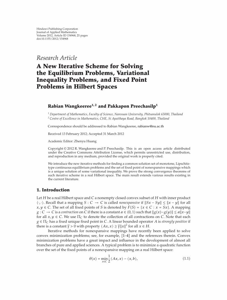
Hindawi Publishing CorporationJournal of Applied MathematicsVolume 2012, Article ID 154968, 21 pagesdoi:10.1155/2012/154968
Research ArticleA New Iterative Scheme for Solvingthe Equilibrium Problems, VariationalInequality Problems, and Fixed PointProblems in Hilbert Spaces
Rabian Wangkeeree1, 2 and Pakkapon Preechasilp1
1 Department of Mathematics, Faculty of Science, Naresuan University, Phitsanulok 65000, Thailand2 Centre of Excellence in Mathematics, CHE, Si Ayutthaya Road, Bangkok 10400, Thailand
Correspondence should be addressed to Rabian Wangkeeree, [email protected]
Received 13 February 2012; Accepted 31 March 2012
Academic Editor: Zhenyu Huang
Copyright q 2012 R. Wangkeeree and P. Preechasilp. This is an open access article distributedunder the Creative Commons Attribution License, which permits unrestricted use, distribution,and reproduction in any medium, provided the original work is properly cited.
We introduce the new iterative methods for finding a common solution set of monotone, Lipschitz-type continuous equilibrium problems and the set of fixed point of nonexpansive mappings whichis a unique solution of some variational inequality. We prove the strong convergence theorems ofsuch iterative scheme in a real Hilbert space. The main result extends various results existing inthe current literature.
1. Introduction
Let H be a real Hilbert space and C a nonempty closed convex subset of H with inner product〈·, ·〉. Recall that a mapping S : C → C is called nonexpansive if ‖Sx − Sy‖ ≤ ‖x − y‖ for allx, y ∈ C. The set of all fixed points of S is denoted by F(S) = {x ∈ C : x = Sx}. A mappingg : C → C is a contraction on C if there is a constant α ∈ (0, 1) such that ‖g(x)−g(y)‖ ≤ α‖x−y‖for all x, y ∈ C. We use ΠC to denote the collection of all contractions on C. Note that eachg ∈ ΠC has a fixed unique fixed point in C. A linear bounded operator A is strongly positive ifthere is a constant γ > 0 with property 〈Ax, x〉 ≥ γ‖x‖2 for all x ∈ H.
Iterative methods for nonexpansive mappings have recently been applied to solveconvex minimization problems; see, for example, [1–4] and the references therein. Convexminimization problems have a great impact and influence in the development of almost allbranches of pure and applied sciences. A typical problem is to minimize a quadratic functionover the set of the fixed points of a nonexpansive mapping on a real Hilbert space:
θ(x) = minx∈C
12〈Ax, x〉 − 〈x, b〉, (1.1)

2 Journal of Applied Mathematics
where A is a linear bounded operator, C is the fixed point set of a nonexpansive mappingT , and b is a given point in H. Let H be a real Hilbert space. Recall that a linear boundedoperator B is strongly positive if there is a constant γ > 0 with property
〈Ax, x〉 ≥ γ‖x‖2 ∀x ∈ H. (1.2)
Recently, Marino and Xu [5] introduced the following general iterative scheme based on theviscosity approximation method introduced by Moudafi [6]:
xn+1 = (I − αnA)Txn + αnγg(xn), n ≥ 0, (1.3)
where A is a strongly positive bounded linear operator on H. They proved that if thesequence {αn} of parameters satisfies appropriate conditions, then the sequence {xn}generated by (1.3) converges strongly to the unique solution of the variational inequality:
⟨(A − γg
)x∗, x − x∗⟩ ≥ 0, x ∈ C, (1.4)
which is the optimality condition for the minimization problem:
minx∈C
12〈Ax, x〉 − h(x), (1.5)
where h is a potential function for γg (i.e., h′(x) = γg(x) for x ∈ H).A mapping B of C into H is called monotone if 〈Bx −By, x −y〉 ≥ 0 for all x, y ∈ C. The
variational inequality problem is to find x ∈ C such that
〈Bx, x − x〉 ≥ 0 ∀x ∈ C. (1.6)
The set of solutions of variational inequality is denoted by VI(C,B). A mapping B : C → His called inverse-strongly monotone if there exists a positive real number β such that
⟨x − y, Bx − By
⟩ ≥ β∥∥Bx − By
∥∥2, ∀x, y ∈ C. (1.7)
For such a case, B is β-inverse-strongly monotone. If B is a β-inverse-strongly monotonemapping of C to H, then it is obvious that B is (1/β)-Lipschitz continuous. In 2009, Klin-eam and Suantai [7] introduced the following general iterative method:
x0 ∈ C, xn+1 = PC
(αnγg(xn) + (I − αnA)SPC(xn − λnBxn)
), n ≥ 0, (1.8)
where PC is the metric projection of H onto C, g is a contraction, A is a strongly positivelinear bounded operator, B is a β-inverse strongly monotone mapping, {αn} ⊂ (0, 1), and{λn} ⊂ [a, b] for some a, b with 0 < a < b < 2β. They proved that under certain appropriateconditions imposed on {αn} and {λn}, the sequence generated by (1.8) converges strongly toa common element of the set of fixed points of nonexpansive mapping and the set of solutions

Journal of Applied Mathematics 3
of the variational inequality for an inverse strongly monotone mapping (say x ∈ C) whichsolves the following variational inequality:
⟨(A − γg
)x, x − x
⟩ ≥ 0, ∀x ∈ F(S) ∩ VI(C,B). (1.9)
We recall the following well-known definitions. A bifunction f : C × C → R is called
(a) monotone on C if
f(x, y)+ f(y, x) ≤ 0, ∀x, y ∈ C; (1.10)
(b) pseudomonotone on C if
f(x, y) ≥ 0 =⇒ f
(y, x) ≤ 0, ∀x, y ∈ C; (1.11)
(c) Lipschitz-type continuous on C with two constants c1 > 0 and c2 > 0 if
f(x, y)+ f(y, z) ≥ f(x, z) − c1
∥∥x − y∥∥2 − c2
∥∥y − z∥∥2
, ∀x, y, z ∈ C. (1.12)
We consider the following equilibrium problems: find x ∈ C such that
Find x ∈ C such that f(x, y) ≥ 0, ∀x ∈ C. (1.13)
The set of solution of problem (1.13) is denoted by EP(f, C). If f(x, y) := 〈Fx, y − x〉 for allx, y ∈ C, where F is a mapping from C to H, then problem EP(f, C) reduces to the variationalinequalities (1.6). It is well known that problem EP(f, C) covers many important problems inoptimization and nonlinear analysis as well as it has found many applications in economic,transportation, and engineering.
For solving the common element of the set of fixed points of a nonexpansive mappingand the solution set of equilibrium problems, S. Takahashi and W. Takahashi [8] introducedthe following viscosity approximation method:
x0 ∈ H,
Find yn ∈ C such that f(yn, y
)+
1rn
⟨y − yn, yn − xn
⟩, ∀x ∈ C,
xn+1 = αng(xn) + (1 − αn)Syn, ∀n ≥ 0,
(1.14)
where {αn} ⊂ [0, 1] and {rn} ⊂ (0,∞). They showed that under certain conditions over{αn} and {rn}, sequences {xn} and {yn} converge strongly to z ∈ F(S) ∩ EP(F), wherez = PF(S)∩EP(F)g(z).

4 Journal of Applied Mathematics
In this paper, inspired and motivated by Klin-eam and Suantai [7] and S. Takahashiand W. Takahashi [8], we introduce the new algorithm for solving the common element ofthe set of fixed points of a nonexpansive mapping, the solution set of equilibrium problems,and the solution set of the variational inequality problems for an inverse strongly monotonemapping. Let f be monotone, Lipschitz-type continuous on C with two constants c1 > 0 andc2 > 0, A a strongly linear bounded operator, and B a β-inverse strongly monotone mapping.Let g : C → C be a contraction with coefficient α such that 0 < γ < γ/α and S : C → C anonexpansive mapping. The algorithm is now described as follows.
Step 1 (initialization). Choose positive sequences {αn} ⊂ (0, 1) and {λn} ⊂ [c, d] for somec, d ∈ (0, 1/L), where L = max{2c1, 2c2} and β ⊂ [a, b] for some a, b with 0 < a < b < 2β.
Step 2 (solving convex problems). For a given point x0 = x ∈ C and set n := 0, we solve thefollowing two strongly convex problems:
yn = argmin{λnf(xn, y
)+
12∥∥y − xn
∥∥2 : y ∈ C
},
tn = argmin{λnf(yn, y
)+
12∥∥y − xn
∥∥2 : y ∈ C
}.
(1.15)
Step 3 (iteration n). Compute
xn+1 = PC
(αnγg(xn) + (I − αnA)SPC
(tn − βBtn
)), (1.16)
where PC is the metric projection of H onto C. Increase n by 1 and go to Step 1.
We show that under some control conditions the sequences {xn}, {yn}, and {tn}defined by (1.15) and (1.16) converge strongly to a common element of solution set ofmonotone, Lipschitz-type continuous equilibrium problems, and the set of fixed points ofnonexpansive mappings which is a unique solution of the variational inequality problem(1.6).
2. Preliminaries
Let C be a nonempty closed convex subset of a real Hilbert space H. Let f : C × C → R
be a bifunction. For solving the mixed equilibrium problem, let us assume the followingconditions for a bifunction f : C × C → R:
(A1) f(x, x) = 0 for all x ∈ C;
(A2) f is Lipschitz-type continuous on C;
(A3) f is monotone on C;
(A4) for each x ∈ C, f(x, ·) is convex and subdifferentiable on C;
(A5) f is upper semicontinuous on C.
The metric (nearest point) projection PC from a Hilbert space H to a closed convex subsetC of H is defined as follows: given x ∈ H, PCx is the only point in C such that
Journal of Applied Mathematics 5
‖x − PCx‖ − inf{‖x − y‖ : y ∈ C}. In what follows lemma can be found in any standardfunctional analysis book.
Lemma 2.1. Let C be a closed convex subset of a real Hilbert spaceH. Given x ∈ H and y ∈ C, then
(i) y = PCx if and only if 〈x − y, y − z〉 ≥ 0 for all z ∈ C,
(ii) PC is nonexpansive,
(iii) 〈x − y, PCx − PCy〉 ≥ ‖PCx − PCy‖2 for all x, y ∈ H,
(iv) 〈x − PCx, PCx − y〉 for all x ∈ H and y ∈ C.
Using Lemma 2.1, one can show that the variational inequality (1.6) is equivalent to afixed point problem.
Lemma 2.2. The point u ∈ C is a solution of the variational inequality (1.6) if and only if u satisfiesthe relation u = PC(u − λBu) for all λ > 0.
A set-valued mapping T : H → 2H is called monotone if for all x, y ∈ H,u ∈ Tx, andv ∈ Ty imply 〈x−y, u−v〉 ≥ 0. A monotone mapping T : H → 2H is maximal if the graph G(T)of T is not property contained in the graph of any other monotone mapping. It is known thata monotone mapping T is maximal if and only if for (x, u) ∈ H×H, 〈x−y, u−v〉 ≥ 0 for every(y, v) ∈ G(T) implies u ∈ Tx. Let B be an inverse-strongly monotone mapping of C to H, letNCv be normal cone to C at v ∈ C, that is, NCv = {w ∈ H : 〈v − u,w〉 ≥ 0, for all u ∈ C},and define
Tv =
⎧⎨
⎩
Bv +NCv, if v ∈ C,
∅, if v /∈ C.(2.1)
Then T is a maximal monotone and 0 ∈ Tv if and only if v ∈ VI(C,B) [9].Now we collect some useful lemmas for proving the convergence results of this paper.
Lemma 2.3 (see [10]). Let C be a nonempty closed convex subset of a real Hilbert space H andh : C → R be convex and subdifferentiable on C. Then x∗ is a solution to the following convexproblem:
min{h(x) : x ∈ C} (2.2)
if and only if 0 ∈ ∂h(x∗) + NC(x∗), where ∂h(·) denotes the subdifferential of h and NC(x∗) is the(outward) normal cone of C at x∗ ∈ C.
Lemma 2.4 (see [11, Lemma 3.1]). Let C be a nonempty closed convex subset of a real Hilbert spaceH. Let f : C × C → R be a pseudomonotone, Lipschitz-type continuous bifunction with constantsc1 > 0 and c2 > 0. For each x ∈ C, let f(x, ·) be convex and subdifferentiable on C. Suppose that thesequences {xn}, {yn}, and {tn} are generated by Scheme (1.15) and p ∈ EP(f). Then
∥∥tn − p∥∥2 ≤ ∥∥xn − p
∥∥2 − (1 − 2λnc1)∥∥xn − yn
∥∥2 − (1 − 2λnc2)∥∥yn − tn
∥∥2, ∀n ≥ 0. (2.3)

6 Journal of Applied Mathematics
Lemma 2.5 (see [12]). Let C be a closed convex subset of a Hilbert space H and let S : C → C be anonexpansive mapping such that F(S)/= ∅. If a sequence {xn} in C such that xn ⇀ z and xn−Sxn →0, then z = Sz.
Lemma 2.6 (see [5]). Assume that A is a strongly positive linear bounded operator on a HilbertspaceH with coefficient γ > 0 and 0 < ρ ≤ ‖A‖−1, then ‖I − ρA‖ ≤ 1 − ργ .
In the following, we also need the following lemma that can be found in the existingliterature [3, 13].
Lemma 2.7 (see [3, Lemma 2.1]). Let {an} be a sequence of non-negative real number satisfyingthe following property:
an+1 ≤ (1 − γn)an + γnβn, n ≥ 0, (2.4)
where {γn} ⊆ (0, 1) and {βn} ⊆ R such that∑∞
n=0 γn = ∞ and lim supn→∞ βn ≤ 0. Then {an}converges to zero, as n → ∞.
3. Main Theorems
In this section, we prove the strong convergence theorem for solving a common elementof solution set of monotone, Lipschitz-type continuous equilibrium problems and the set offixed points of nonexpansive mappings.
Theorem 3.1. LetH be a real Hilbert space, and letC be a closed convex subset ofH. Let f : C×C →R be a bifunction satisfying (A1)–(A5), let B : C → H be a β-inverse strongly monotone mapping,let A be a strongly positive linear bounded operator of H into itself with coefficient γ > 0 such that‖A‖ = 1 and let g : C → C be a contraction with coefficient α(α ∈ (0, 1)). Assume that 0 < γ < γ/α.Let S be a nonexpansive mapping of C into itself such thatΩ := F(S) ∩ EP(f) ∩VI(C,B)/= ∅. Let thesequences {xn}, {yn}, and {tn} be generated by (1.15) and (1.16), where {αn} ⊂ (0, 1), {β} ⊂ [a, b]for some a, b ∈ (0, 2β), and {λn} ⊂ [c, d] for some c, d ∈ (0, 1/L), where L = max{2c1, 2c2}.Suppose that the following conditions are satisfied:
(B1) limn→∞ αn = 0;
(B2)∑∞
n=1 αn = ∞;
(B3)∑∞
n=1 |αn+1 − αn| < ∞;
(B4)∑∞
n=1
√|λn+1 − λn| < ∞.
Then the following holds.
(i) PΩ(I −A + γg) is a contraction on C; hence there exists q ∈ C such that q = PΩ(I −A +γg)(q), where PΩ is the metric projection of H onto C.
(ii) The sequences {xn}, {yn}, and {tn} converge strongly to the same point q.

Journal of Applied Mathematics 7
Proof. For any x, y ∈ H, we have
∥∥PΩ(γg + (I −A)
)x − PΩ
(γg + (I −A)
)y∥∥ ≤ ∥∥γg + (I −A)x − (γg + (I −A)
)y∥∥
≤ γ∥∥g(x) − g
(y)∥∥ + ‖I −A‖∥∥x − y
∥∥
≤ γα∥∥x − y
∥∥ +(1 − γ
)∥∥x − y∥∥
=(1 − (γ − γα
))∥∥x − y∥∥.
(3.1)
Banach’s contraction principle guarantees that PΩ(γg + (I −A)) has a unique fixed point, sayq ∈ H. That is, q = PΩ(γg + (I −A))(q). By Lemma 2.1(i), we obtain that
⟨(γg −A
)q, p − q
⟩ ≤ 0, ∀p ∈ Ω. (3.2)
The proof of (ii) is divided into several steps.
Step 1. I − βB is nonexpansive mapping. Indeed, since B is a β-strongly monotone mappingand 0 < β < 2β, for all x, y ∈ C, we have
∥∥∥(I − βB
)x −(I − βB
)y∥∥∥
2=∥∥∥(x − y
) − β(Bx − By
)∥∥∥2
=∥∥x − y
∥∥2 − 2β⟨x − y, Bx − By
⟩+ β
2∥∥Bx − By∥∥2
≤ ∥∥x − y∥∥2 − 2β
∥∥Bx − By∥∥2 + β
2∥∥Bx − By∥∥2
≤ ∥∥x − y∥∥2 + β
(β − 2β
)∥∥Bx − By∥∥2
≤ ∥∥x − y∥∥2
.
(3.3)
Step 2. We show that {xn} is a bounded sequence. Put wn = PC(tn − βBtn) for all n ≥ 0. Letp ∈ Ω; we have
∥∥wn − p∥∥ =∥∥∥PC
(tn − βBtn
)− PC
(p − βBp
)∥∥∥
≤∥∥∥(I − βB
)tn −
(I − βB
)p∥∥∥
≤ ∥∥tn − p∥∥.
(3.4)
By Lemma 2.4, we have
∥∥xn+1 − p∥∥ =∥∥PC
(αnγg(xn) + (I − αnA)S(wn)
) − p∥∥
≤ ∥∥αnγg(xn) + (I − αnA)S(wn) − p∥∥
≤ αn
∥∥γg(xn) −Ap∥∥ + ‖I − αnA‖∥∥S(wn) − S
(p)∥∥

8 Journal of Applied Mathematics
≤ αn
∥∥γg(xn) −Ap
∥∥ + ‖I − αnA‖∥∥wn − p
∥∥
≤ αn
∥∥γg(xn) −Ap
∥∥ +(1 − αnγ
)∥∥tn − p∥∥
≤ αn
∥∥γg(xn) −Ap
∥∥ +(1 − αnγ
)∥∥xn − p∥∥
≤ αnγα∥∥xn − p
∥∥ + αn
∥∥γg(p) −Ap
∥∥ +(1 − αnγ
)∥∥xn − p∥∥
≤ (1 − αn
(γ − γα
))∥∥xn − p∥∥ + αn
(γ − γα
)∥∥γg(p) −Ap
∥∥
γ − γα.
(3.5)
By induction, we get that
∥∥xn − p∥∥ ≤ max
{∥∥x1 − p∥∥,
1γ − γα
∥∥γg(p) −Ap
∥∥}, n ≥ 0. (3.6)
Hence {xn} is bounded, and then {wn}, {yn}, and {tn} are also bounded.
Step 3. We show that
limn→∞
‖xn+1 − xn‖ = 0. (3.7)
Since f(x, ·) is convex on C for each x ∈ C, applying Lemma 2.3, we see that tn =argmin{(1/2)‖t − xn‖ + λnf(yn, t) : t ∈ C} if and only if
0 ∈ ∂2
(λnf(yn, t)+
12∥∥y − xn
∥∥2)(tn) +NC(tn), (3.8)
where NC(x) is the (outward) normal cone of C at x ∈ C. This implies that 0 = λnw+tn−xn+w,where w ∈ ∂2f(yn, tn) and w ∈ NCtn. By the definition of the normal cone NC, we have
〈xn − λnw − tn, t − tn〉 = 〈w, t − tn〉 ≤ 0, ∀t ∈ C, (3.9)
and so
〈tn − xn, t − tn〉 ≥ λn〈w, tn − t〉, ∀t ∈ C. (3.10)
Substituting t = tn+1 ∈ C into (3.10), we get that
〈tn − xn, tn+1 − tn〉 ≥ λn〈w, tn − tn+1〉. (3.11)
Since f(x, ·) is subdifferentiable on C and w ∈ ∂2f(yn, tn), we have
f(yn, t) − f
(yn, tn
) ≥ 〈w, t − tn〉, ∀t ∈ C. (3.12)

Journal of Applied Mathematics 9
From (3.11) and (3.12), we obtain that
〈tn − xn, tn+1 − tn〉 ≥ λn〈w, tn − tn+1〉≥ λn
(f(yn, tn
) − f(yn, tn+1
)).
(3.13)
By the similar way, we also have
〈tn+1 − xn+1, tn − tn+1〉 ≥ λn+1(f(yn+1, tn+1
) − f(yn+1, tn
)). (3.14)
It follows from (3.13) and (3.14) and f is Lipschitz-type continuous and monotone, we get
12‖xn+1 − xn‖2 − 1
2‖tn+1 − tn‖2 ≥ 〈tn+1 − tn, tn − xn − tn+1 + xn+1〉
≥ λn(f(yn, tn
) − f(yn, tn+1
))+ λn+1
(f(yn+1, tn+1
) − f(yn+1, tn
))
≥ λn(−f(tn, tn+1) − c1
∥∥yn − tn∥∥2 − c2‖tn − tn+1‖2
)
+ λn+1
(−f(tn+1, tn) − c1
∥∥yn+1, tn+1∥∥2 − c2‖tn − tn+1‖2
)
≥ (λn+1 − λn)f(tn, tn+1)
≥ −|λn+1 − λn|∣∣f(tn, tn+1)
∣∣,(3.15)
and hence
‖tn+1 − tn‖2 =√‖xn+1 − xn‖2 + 2|λn+1 − λn|
∣∣f(tn, tn+1)∣∣
≤ ‖xn+1 − xn‖√
2|λn+1 − λn|∣∣f(tn, tn+1)
∣∣.
(3.16)
Thus, we have
‖xn+1 − xn‖=∥∥PC
(αnγg(xn) + (I − αnA)S(wn)
) − PC
(αn−1γg(xn−1) + (I − αn−1A)S(wn−1)
)∥∥
≤ ∥∥αnγg(xn) + (I − αnA)S(wn) − αn−1γg(xn−1) − (I − αn−1A)S(wn−1)∥∥
=∥∥αnγg(xn) − αnγg(xn−1) + αnγg(xn−1) − αn−1γg(xn−1) + (I − αnA)S(tn)
−(I − αnA)S(tn−1) + (I − αnA)S(tn−1) − (I − αn−1A)S(tn−1)‖≤ αnγα‖xn − xn−1‖ + |αn − αn−1|
∥∥γg(xn−1)∥∥
+ ‖I − αnA‖‖S(wn) − S(wn−1)‖ + |αn − αn−1|‖AS(tn−1)‖≤ αnγα‖xn − xn−1‖ +
∥∥I − αnγ∥∥‖wn −wn−1‖ + |αn − αn−1|
(γ∥∥g(xn−1)
∥∥ + ‖AS(tn−1)‖)

10 Journal of Applied Mathematics
≤ αnγα‖xn − xn−1‖ +∥∥I − αnγ
∥∥‖tn − tn−1‖ + |αn − αn−1|
(γ∥∥g(xn−1)
∥∥ + ‖AS(tn−1)‖
)
≤ αnγα‖xn − xn−1‖ +(1 − αnγ
)(‖xn − xn−1‖ +
√2|λn+1 − λn|
∣∣f(tn, tn+1)
∣∣)
+ |αn − αn−1|(γ∥∥g(xn−1)
∥∥ + ‖AS(tn+1)‖
)
≤ (1 − αn
(γ − γα
))‖xn − xn−1‖ +(1 − αnγ
)√2|λn+1 − λn|K + |αn − αn−1|M,
(3.17)
where K ≥ supn≥0
√|f(tn−1, tn)| and M ≥ supn≥0γ‖g(xn−1)‖+‖AS(tn−1)‖. Using (B3), (B4), and
Lemma 2.7, we have limn→∞‖xn+1 − xn‖ = 0.
Step 4. We show that
limn→∞
‖xn − tn‖ = 0. (3.18)
Indeed, for each p ∈ Ω, applying Lemma 2.4, we have
∥∥xn+1 − p∥∥2
=∥∥PC
(αnγg(xn) + (I − αnA)S(wn)
) − p∥∥2
≤ ∥∥αnγg(xn) + (I − αnA)S(wn) − p∥∥2
≤ (αn
∥∥γg(xn) −Ap∥∥ + (1 − αnγ)
∥∥S(wn) − p∥∥)2
= α2n
∥∥γg(xn) −Ap∥∥2 +
(1 − αnγ
)2∥∥S(wn) − p∥∥2
+ 2αn
(1 − αnγ
)∥∥γg(xn) − g(p)∥∥∥∥S(wn) − p
∥∥
≤ αn
∥∥γg(xn) −Ap∥∥2 +
(1 − αnγ
)∥∥S(wn) − p∥∥2
+ 2αn
(1 − αnγ
)∥∥γg(xn) − g(p)∥∥∥∥S(wn) − p
∥∥
≤ αn
(∥∥γg(xn) − γg(p)∥∥ +
∥∥γg(p) −Ap
∥∥)2 +(1 − αnγ
)∥∥S(wn) − p∥∥2
+ 2αn
(1 − αnγ
)∥∥γg(xn) − g(p)∥∥∥∥S(wn) − p
∥∥
= αn
∥∥γg(xn) − γg(p)∥∥2 + 2αn
∥∥γg(xn) − γg(p)∥∥∥∥γg
(p) −Ap
∥∥ + αn
∥∥γg(p) −Ap∥∥2
+(1 − αnγ
)∥∥S(wn) − p∥∥2 + 2αn
(1 − αnγ
)∥∥γg(xn) − g(p)∥∥∥∥S(wn) − p
∥∥
≤ αn
∥∥γg(xn) − γg(p)∥∥2 +
(1 − αnγ
)∥∥tn − p∥∥2 + θn
≤ αnγ2α2∥∥xn − p
∥∥2 + θn
+(1 − αnγ
)(∥∥xn − p∥∥2 − (1 − 2λnc1)
∥∥xn − yn
∥∥2 − (1 − 2λnc2)∥∥yn − tn
∥∥2)

Journal of Applied Mathematics 11
≤ αn
(γα)2∥∥xn − p
∥∥2 +
(1 − αnγ
)∥∥xn − p∥∥2 − (1 − αnγ
)(1 − 2λnc1)
∥∥xn − yn
∥∥2
− (1 − αnγ)(1 − 2λnc2)
∥∥yn − tn
∥∥2 + θn
=(
1 − αn
(γ − (γα)2
))∥∥xn − p
∥∥2 − (1 − αnγ
)(1 − 2λnc1)
∥∥xn − yn
∥∥2
− (1 − αnγ)(1 − 2λnc2)
∥∥yn − tn
∥∥2 + θn
≤ ∥∥xn − p∥∥2 − (1 − αnγ
)(1 − 2λnc1)
∥∥xn − yn
∥∥2 − (1 − αnγ
)(1 − 2λnc2)
∥∥yn − tn
∥∥2
+ θn,
(3.19)
where
θn = 2αn
∥∥γg(xn) − γg(p)∥∥∥∥γg
(p) −Ap
∥∥ + 2αn
(1 − αnγ
)∥∥γg(xn) − g(p)∥∥
× ∥∥S(wn) − p∥∥ + αn
∥∥γg(p) −Ap
∥∥2.
(3.20)
It then follows that(1 − αnγ
)(1 − 2λnc2)
∥∥xn − yn
∥∥2 ≤ ∥∥xn − p∥∥2 − ∥∥xn+1 − p
∥∥2
− (1 − αnγ)(1 − 2λnc1)
∥∥yn − tn∥∥2 + θn
≤ (∥∥xn − p∥∥ +∥∥xn+1 − p
∥∥)‖xn − xn+1‖ + θn −→ 0,
(3.21)
as n → ∞. Hence
limn→∞
∥∥xn − yn
∥∥ = 0. (3.22)
By the similar way, also
limn→∞
∥∥yn − tn∥∥ = 0. (3.23)
From (3.22) and (3.23), we can conclude that
‖xn − tn‖ ≤ ∥∥xn − yn
∥∥ +∥∥yn − tn
∥∥ −→ 0 as n −→ ∞. (3.24)
Step 5. We show that
limn→∞
‖xn − Sxn‖ = 0. (3.25)
From (1.15), we get that
∥∥xn+1 − p∥∥2 =
∥∥PC
(αnγg(xn) + (I − αnA)Swn
) − p∥∥2
≤ ∥∥αnγg(xn) + (I − αnA)Swn − p∥∥2

12 Journal of Applied Mathematics
≤ (αn
∥∥γg(xn) −Ap
∥∥ +(1 − αnγ
)∥∥Swn − p∥∥)2
≤ αn
∥∥γg(xn) −Ap
∥∥2 +
(1 − αnγ
)∥∥wn − p∥∥2
+ 2αn
(1 − αnγ
)∥∥γg(xn) −Ap∥∥∥∥wn − p
∥∥
≤ αn
∥∥γg(xn) −Ap
∥∥2 +
(1 − αnγ
)∥∥∥(I − βB
)tn −
(I − βB
)p∥∥∥
2
+ 2αn
(1 − αnγ
)∥∥γg(xn) −Ap∥∥∥∥wn − p
∥∥
≤ αn
∥∥γg(xn) −Ap
∥∥2 +
(1 − αnγ
)(∥∥tn − p∥∥2 + β
(β − 2β
)∥∥Btn − Bp
∥∥2)
≤ αn
∥∥γg(xn) −Ap
∥∥2 +
∥∥tn − p
∥∥2 +
(1 − αnγ
)a(b − 2β
)∥∥Btn − Bp∥∥2
+ 2αn
(1 − αnγ
)∥∥γg(xn) −Ap∥∥∥∥wn − p
∥∥
≤ αn
∥∥γg(xn) −Ap∥∥2 +
∥∥xn − p∥∥2 +
(1 − αnγ
)a(b − 2β
)∥∥Btn − Bp∥∥2
+ 2αn
(1 − αnγ
)∥∥γg(xn) −Ap∥∥∥∥wn − p
∥∥,
(3.26)
and hence
−(1 − αnγ)a(b − 2β
)∥∥Btn − Bp∥∥2 ≤ αn
∥∥γg(xn) −Ap∥∥ +∥∥xn − p
∥∥2 − ∥∥xn+1 − p∥∥2
+ 2αn
(1 − αnγ
)∥∥γg(xn) −Ap∥∥∥∥wn − p
∥∥.(3.27)
Since αn → 0, we get that ‖Btn − Bp‖ → 0, as n → ∞. By Lemma 2.1(iii), we have
∥∥wn − p∥∥2
=∥∥∥PC
(tn − βBtn
)− PC
(p − βBp
)∥∥∥2
≤⟨(
tn − βBtn)−(p − βBp
), wn − p
⟩
=12
(∥∥∥(tn − βBtn
)−(p − βBp
)∥∥∥2+∥∥wn − p
∥∥2−∥∥∥(tn − βBtn
)−(tn − βBtn
)−(wn − p
)∥∥∥2)
≤ 12
(∥∥tn − p∥∥2 +
∥∥wn − p∥∥2 −
∥∥∥(tn −wn) − β(Btn − Bp
)∥∥∥2)
≤ 12
(∥∥tn − p∥∥2 +
∥∥wn − p∥∥2 − ‖tn −wn‖2
)+
12
(2β⟨tn −wn, Btn − Bp
⟩ − β2n
∥∥Btn − Bp∥∥2),
(3.28)
which implies that
∥∥wn − p∥∥2 ≤ ∥∥tn − p
∥∥2 − ‖tn −wn‖2 + 2β⟨tn −wn, Btn − Bp
⟩ − β2n
∥∥Btn − Bp∥∥2. (3.29)

Journal of Applied Mathematics 13
Again from (3.29), we have
∥∥xn+1 − p
∥∥2 =
∥∥PC
(αnγg(xn) + (I − αnA)Swn
) − p∥∥2
≤ ∥∥αnγg(xn) + (I − αnA)Swn − p∥∥2
≤ (αn
∥∥γg(xn) −Ap
∥∥ +(1 − αnγ
)∥∥Swn − p∥∥)2
≤ αn
∥∥γg(xn) −Ap
∥∥2 +
(1 − αnγ
)∥∥wn − p∥∥2
+ 2αn
(1 − αnγ
)∥∥γg(xn) −Ap∥∥∥∥wn − p
∥∥
≤ αn
∥∥γg(xn) −Ap
∥∥2 +
(1 − αnγ
)∥∥tn − p∥∥2 − (1 − αnγ
)‖tn −wn‖2
+ 2β(1 − αnγ
)⟨tn −wn, Btn − Bp
⟩ − β2n
(1 − αnγ
)∥∥Btn − Bp∥∥2
+ 2αn
(1 − αnγ
)∥∥γg(xn) −Ap∥∥∥∥wn − p
∥∥
≤ αn
∥∥γg(xn) −Ap∥∥2 +
∥∥xn − p∥∥2 − (1 − αnγ
)‖tn −wn‖2
+ 2β(1 − αnγ
)⟨tn −wn, Btn − Bp
⟩ − β2n
(1 − αnγ
)∥∥Btn − Bp∥∥2
+ 2αn
(1 − αnγ
)∥∥γg(xn) −Ap∥∥∥∥wn − p
∥∥.
(3.30)
This implies that
(1 − αnγ
)‖tn −wn‖2 ≤ αn
∥∥γg(xn) −Ap∥∥2 +
∥∥xn − p∥∥2 − ∥∥xn+1 − p
∥∥2
+ 2β(1 − αnγ
)⟨tn −wn, Btn − Bp
⟩ − β2n
(1 − αnγ
)∥∥Btn − Bp∥∥2
+ 2αn
(1 − αnγ
)∥∥γg(xn) −Ap∥∥∥∥wn − p
∥∥.
(3.31)
Since αn → 0 and ‖Btn − Bp‖ → 0, we obtain that
limn→∞
‖tn −wn‖ = 0. (3.32)
From (1.16), we have
‖xn+1 − Swn‖ =∥∥PC
(αnγg(xn) + (I − αnA)Swn
) − PC(Swn)∥∥
≤ ∥∥αnγg(xn) + (I − αnA)Swn − Swn
∥∥
= αn
∥∥γg(xn) +ASwn
∥∥ −→ 0, as n −→ ∞.
(3.33)
Since
‖tn − Stn‖ ≤ ‖tn − xn‖ + ‖xn − xn+1‖ + ‖xn+1 − Swn‖ + ‖Swn − Stn‖≤ ‖tn − xn‖ + ‖xn − xn+1‖ + ‖xn+1 − Swn‖ + ‖wn − tn‖,
(3.34)

14 Journal of Applied Mathematics
from (3.7), (3.24), (3.32), and (3.33), we obtain that ‖tn − Stn‖ → 0, as n → ∞. Moreover, weget that
‖wn − Swn‖ ≤ ‖wn − tn‖ + ‖tn − Stn‖ + ‖Stn − Swn‖≤ 2‖wn − tn‖ + ‖tn − Stn‖ −→ 0, as n −→ ∞.
(3.35)
Since
‖xn −wn‖ ≤ ‖xn − tn‖ + ‖tn −wn‖, (3.36)
it implies that
limn→∞
‖xn −wn‖ = 0. (3.37)
Since
‖xn − Sxn‖ ≤ ‖xn − xn+1‖ + ‖xn+1 − Swn‖ + ‖Swn − Sxn‖≤ ‖xn − xn+1‖ + ‖xn+1 − Swn‖ + ‖wn − xn‖,
(3.38)
we obtain that
limn→∞
‖xn − Sxn‖ = 0. (3.39)
Step 6. We show that
lim supn→∞
⟨(γg −A
)q, Swn − q
⟩ ≤ 0. (3.40)
Indeed, we choose a subsequence {wnk} of {wn} such that
lim supn→∞
⟨(γg −A
)q, Swn − q
⟩= lim
k→∞⟨(γg −A
)q, Swnk − q
⟩. (3.41)
Since {wn} is bounded, there exists a subsequence {wnki} of {wnk} which converges weakly
to p. Next we show that p ∈ Ω.We prove that p ∈ F(S). We may assume without loss of generality that wnk ⇀ p.
Since ‖wn − Swn‖ → 0, we obtain Swnk ⇀ p. Since ‖xn − Sxn‖ → 0, ‖xn −wn‖ → 0 and byLemma 2.5, we have p ∈ F(S).
We show that p ∈ EP(f). From Steps 4 and 6, we have that
tnk ⇀ p, xnk ⇀ p, ynk ⇀ p. (3.42)

Journal of Applied Mathematics 15
Since yn is the unique solution of the convex minimization problem
min{
12∥∥y − xn
∥∥2 + f
(xn, y
): y ∈ C
}, (3.43)
we have
0 ∈ ∂2
(λnf(xn, y
)+
12∥∥y − xn
∥∥2)(yn
)+NC
(yn
). (3.44)
It follows that
0 = λnz + yn − xn + zn, (3.45)
where z ∈ ∂2f(xn, yn) and zn ∈ NC(yn). By the definition of the normal cone NC, we get that
⟨yn − xn, y − yn
⟩ ≥ λn⟨z, yn − y
⟩, ∀y ∈ C. (3.46)
On the other hand, since f(xn, ·) is subdifferentiable on C and z ∈ ∂2f(xn, yn), we have
f(xn, y
) − f(xn, yn
) ≥ ⟨z, y − yn
⟩, ∀y ∈ C. (3.47)
Combining (3.47) with (3.46), we have
λn(f(xn, y
) − f(xn, yn
)) ≥ ⟨yn − xn, yn − y⟩, ∀y ∈ C. (3.48)
Hence
λnk
(f(xnk , y
) − f(xnk , ynk
)) ≥ ⟨ynk − xnk , ynk − y⟩, ∀y ∈ C. (3.49)
Thus, using {λ ⊂ [a, b] ⊂ (0, 1/L)} and the upper semicontinuity of f , we have
f(p, y) ≥ 0, ∀y ∈ C. (3.50)
Hence p ∈ EP(f).We show that p ∈ VI(C,B). Let
Tv =
⎧⎨
⎩
Bv +NCv, v ∈ C,
∅, v /∈ C,(3.51)

16 Journal of Applied Mathematics
where NCv is normal cone to C at v ∈ C. Then T is a maximal monotone operator. Let (v, u) ∈G(T). Since u − Bv ∈ NCv and wn ∈ C, we have 〈v − yn, u − Bv〉 ≥ 0. On the other hand, byLemma 2.1(iv) and from wn = PC(tn − βBtn), we have
⟨v −wn,wn −
(tn − βBtn
)⟩≥ 0, (3.52)
and hence 〈v −wn, (wn − tn)/β + Btn〉 ≥ 0. Therefore, we get that
〈v −wnk , u〉 ≥ 〈v −wnk , Bv〉
≥ 〈v −wnk , Bv〉 −⟨v −wnk ,
wnk − tnk
λnk
+ Bxnk
⟩
=⟨v −wnk , Bv − Btnk −
wnk − tnk
λnk
⟩
= 〈v −wnk , Bv − Bwnk〉 + 〈v −wnk , Bwnk − Btnk〉 −⟨v −wnk ,
wnk − tnk
λnk
⟩
≥ 〈v −wnk , Bwnk − Btnk〉 −⟨v −wnk ,
wnk − tnk
λnk
⟩.
(3.53)
This implies that 〈v − p, u〉 ≥ 0 as k → ∞. Since T is maximal monotone, we have p ∈ T−10and hence p ∈ VI(C,B).
From (a), (b), and (c), we obtain that p ∈ Ω. This implies that
lim supn→∞
〈(γg −A)q, Swn − q〉 = lim
k→∞〈(γg −A
)q, Swnk − q〉
= 〈(γg −A)q, p − q〉 ≤ 0.
(3.54)
Step 7. We show that xn → q. We observe that
∥∥xn+1 − q∥∥2 =
∥∥PC
(αnγg(xn) + (I − αnA)Swn
) − PC(q)∥∥2
≤ ∥∥αnγg(xn) + (I − αnA)Swn − q∥∥2
≤ α2n
∥∥γg(xn) −Aq∥∥ +∥∥(I − αnA)
(Swn − q
)∥∥2
+ 2αn
⟨(I − αnA)
(Swn − q
), γg(xn) −Aq
⟩
≤ α2n
∥∥γg(xn) −Aq∥∥ +(1 − αnγ
)2∥∥Swn − q∥∥2
+ 2αn
⟨Swn − q, γg(xn) −Aq
⟩ − 2α2n
⟨A(Swn − q
), γg(xn) −Aq
⟩
≤ (1 − αnγ)2∥∥wn − q
∥∥2 + α2n
∥∥γg(xn) −Aq∥∥
+ 2αn
⟨Swn − q, γg(xn) − γg
(q)⟩
+ 2αn
⟨Swn − q, γg
(q) −Aq
⟩
− 2α2n
⟨A(Swn − q
), γg(xn) −Aq
⟩

Journal of Applied Mathematics 17
≤ (1 − αnγ)2∥∥tn − q
∥∥2 + α2
n
∥∥γg(xn) −Aq
∥∥
+ 2αn
∥∥Swn − q
∥∥∥∥γg(xn) − γg
(q)∥∥ + 2αn
⟨Swn − q, γg
(q) −Aq
⟩
− 2α2n
⟨A(Swn − q
), γg(xn) −Aq
⟩
≤ (1 − αnγ)2∥∥xn − q
∥∥2 + α2
n
∥∥γg(xn) −Aq
∥∥
+ 2γααn
∥∥wn − q
∥∥∥∥xn − q
∥∥ + 2αn
⟨Swn − q, γg
(q) −Aq
⟩
− 2α2n
⟨A(Swn − q
), γg(xn) −Aq
⟩
≤ (1 − αnγ)2∥∥xn − q
∥∥2 + α2
n
∥∥γg(xn) −Aq
∥∥2
+ 2γααn
∥∥xn − q
∥∥2 + 2αn
⟨Swn − q, γg
(q) −Aq
⟩
− 2α2n
⟨A(Swn − q
), γg(xn) −Aq
⟩
≤((
1 − αnγ)2 + 2γααn
)∥∥xn − q∥∥2 + α2
n
∥∥γg(xn) −Aq∥∥2
+ 2αn
⟨Swn − q, γg
(q) −Aq
⟩+ α2
nγ2∥∥xn − q
∥∥2
+ 2α2n
∥∥A(Swn − q
)∥∥∥∥Aq − γg(xn)∥∥
=(1 − 2αn
(γ − γα
))∥∥xn − q∥∥2
+ αn
(2⟨Swn − q, γg
(q) −Aq
⟩+ αn
∥∥γg(xn) −Aq∥∥2
+2αn
∥∥A(Swn − q
)∥∥∥∥Aq − γg(xn)∥∥ + αnγ
2∥∥xn − q∥∥2).
(3.55)
Since {xn}, {g(xn)}, and ‖Swn‖ are bounded, we can take a constant M > 0 such that
M ≥ supn≥0
{αn
∥∥γg(xn) −Aq∥∥2 + 2αn
∥∥A(Swn − q
)∥∥∥∥Aq − γg(xn)∥∥ + αnγ
2∥∥xn − q∥∥2}. (3.56)
This implies that
∥∥xn+1 − q∥∥2 ≤ (1 − 2
(γ − γα
)αn
)∥∥xn − q∥∥2 + αnσn, (3.57)
where σn = 2〈Swn −q, γg(q)−Aq〉+Mαn. From (3.40), we have lim supn→∞σn ≤ 0. ApplyingLemma 2.7 to (3.57), we obtain that xn → q as n → ∞. This completes the proof.
If we put γ = 1 and A = I in Theorem 3.1, we immediately obtain the followingcorollary.
Corollary 3.2. LetH be a real Hilbert space, and letC be a closed convex subset ofH. Let f : C×C →R be a bifunction satisfying (A1)–(A5), let B : C → H be a β-inverse strongly monotone mapping,and let g : C → C be a contraction with coefficient α (α ∈ (0, 1)). Assume that 0 < γ < γ/α. Let

18 Journal of Applied Mathematics
S be a nonexpansive mapping of C into itself such that Ω := F(S) ∩ EP(f) ∩ VI(C,B)/= ∅. Let thesequences {xn}, {yn}, and {tn} be generated by
x0 = x ∈ C,
yn = argmin{λnf(xn, y
)+
12∥∥y − xn
∥∥2 : y ∈ C
},
tn = argmin{λnf(yn, y
)+
12∥∥y − xn
∥∥2 : y ∈ C
},
xn+1 = αng(xn) + (1 − αn)SPC
(tn − βBtn
), n ≥ 0,
(3.58)
where {αn} ⊂ (0, 1), {β} ⊂ [a, b] for some a, b ∈ (0, 2β), and {λn} ⊂ [c, d] for some c, d ∈ (0, 1/L),where L = max{2c1, 2c2}. Suppose that the following conditions are satisfied:
(B1) limn→∞αn = 0;
(B2)∑∞
n=1 αn = ∞;
(B3)∑∞
n=1 |αn+1 − αn| < ∞;
(B4)∑∞
n=1
√|λn+1 − λn| < ∞.
Then the following holds.
(i) PΩg is a contraction on C; and hence there exists q ∈ C such that q = PΩg(q), where PΩ isthe metric projection of H onto C.
(ii) The sequences {xn}, {yn}, and {tn} converge strongly to the same point q which is theunique solution in the Ω to the following variational inequality:
⟨(I − f
)q, x − q
⟩ ≥ 0, ∀x ∈ Ω. (3.59)
If we put g ≡ u in the previous corollary, we get the following corollary.
Corollary 3.3. Let H be a real Hilbert space, and let C be a closed convex subset of H. Let f :C × C → R be a bifunction satisfying (A1)–(A5), and let B : C → H be a β-inverse stronglymonotone mapping. Assume that 0 < γ < γ/α. Let S be a nonexpansive mapping of C into itself suchthat Ω := F(S) ∩ EP(f) ∩ VI(C,B)/= ∅. Let the sequences {xn}, {yn}, and {tn} be generated by
x0 = x ∈ C,
yn = argmin{λnf(xn, y
)+
12∥∥y − xn
∥∥2 : y ∈ C
},
tn = argmin{λnf(yn, y
)+
12∥∥y − xn
∥∥2 : y ∈ C
},
xn+1 = αnu + (1 − αn)SPC
(tn − βBtn
), n ≥ 0,
(3.60)

Journal of Applied Mathematics 19
where {αn} ⊂ (0, 1), {β} ⊂ [a, b] for some a, b ∈ (0, 2β), and {λn} ⊂ [c, d] for some c, d ∈ (0, 1/L),where L = max{2c1, 2c2}. Suppose that the following conditions are satisfied:
(B1) limn→∞ αn = 0;
(B2)∑∞
n=1 αn = ∞;
(B3)∑∞
n=1 |αn+1 − αn| < ∞;
(B4)∑∞
n=1
√|λn+1 − λn| < ∞.
Then the sequences {xn}, {yn}, and {tn} converge strongly to the same point q, where q = PΩu, whichis the unique solution in the Ω to the following variational inequality:
⟨q − u, x − q
⟩ ≥ 0, ∀x ∈ Ω. (3.61)
4. Deduced Theorems
Let C be a nonempty closed convex subset of a real Hilbert space H with inner product 〈·, ·〉.Let F be a nonlinear mapping from C into H. Recall that the function F is called
(a) strongly monotone on C if there exists β > 0 such that
⟨F(x) − F
(y), x − y
⟩ ≥ β∥∥x − y
∥∥2, ∀x, y ∈ C; (4.1)
(b) monotone on C if⟨F(x) − F
(y), x − y
⟩ ≥ 0, ∀x, y ∈ C; (4.2)
(c) pseudomonotone on C if
⟨F(y), x − y
⟩ ≥ 0 =⇒ ⟨F(x), x − y⟩ ≤ 0, ∀x, y ∈ C. (4.3)
Remark 4.1. Notice that if F is L-Lipschitz on C, then for each x, y ∈ C, f(x, y) = 〈F(x), y−x〉is Lipschitz-type continuous with constants c1 = c2 = L/2 on C. Indeed,
f(x, y)+ f(y, z) − f(x, z) = 〈F(x), y − x〉 + ⟨F(y), z − y
⟩ − 〈F(x), z − x〉= −⟨F(y) − F(x), y − z
⟩
≥ −∥∥F(y) − F(x)∥∥∥∥y − z
∥∥
≥ −L∥∥x − y∥∥∥∥y − z
∥∥
≥ −L2∥∥x − y
∥∥2 − L
2∥∥y − z
∥∥2
= −c1∥∥x − y
∥∥2 − c2∥∥y − z
∥∥2.
(4.4)
Thus f is Lipschitz-type continuous on C.

20 Journal of Applied Mathematics
Let f : C × C → R be defined by f(x, y) = 〈F(x), y − x〉, where F : C → H. Thus, byAlgorithm (1.15), we get the following:
yn = argmin{λnf(xn, y
)+
12∥∥y − xn
∥∥2 : y ∈ C
}
= argmin{λn⟨F(xn), y − xn
⟩+
12∥∥y − xn
∥∥2 : y ∈ C
}
= PC(xn − λnF(xn)).
(4.5)
Similarly, we also obtain that tn = PC(xn − λnF(yn)). Applying Theorem 3.1, we obtainthe convergence theorem for finding a common element of the set of fixed points of anonexpansive mapping and the solution set VI(C,B).
Corollary 4.2. LetH be a real Hilbert space, and letC be a closed convex subset ofH. Let F : C → Hbe a monotone, L-Lipschitz continuous mapping, let B : C → H be a β-inverse strongly monotonemapping, also let A be a strongly positive linear bounded operator of H into itself with coefficientγ > 0 such that ‖A‖ = 1, and let g : C → C be a contraction with coefficient α (α ∈ (0, 1)). Assumethat 0 < γ < γ/α. Let S be a nonexpansive mapping of C into itself such that Ω = F(S) ∩ EP(f) ∩VI(C,B)/= ∅. Let the sequence {xn}, {yn}, and {tn} be generated by
x0 = x ∈ C,
yn = PC(xn − λnF(xn)),
tn = PC
(xn − λnF
(yn
)),
xn+1 = PC
(αnγg(xn) + (I − αnA)SPC
(tn − βBtn
)), n ≥ 0,
(4.6)
where {αn} ⊂ (0, 1), {β} ⊂ [a, b] for some a, b ∈ (0, 2β), and {λn} ⊂ [c, d] for some c, d ∈ (0, 1/L).Suppose that the following conditions are satisfied:
(B1) limn→∞ αn = 0;
(B2)∑∞
n=1 αn = ∞;
(B3)∑∞
n=1 |αn+1 − αn| < ∞;
(B4)∑∞
n=1
√|λn+1 − λn| < ∞.
Then the sequences {xn}, {yn}, and {tn} converge strongly to the same point q, where q = PΩ(I −A+γg)(q).
Coflict of Interests
The authors declare that they have no conflict interests.
Authors’ Contribution
All authors read and approved the final paper.

Journal of Applied Mathematics 21
Acknowledgments
The authors would like to thank the referees for reading this paper carefully, providingvaluable suggestions and comments, and pointing out a major error in the original version ofthis paper. Finally, the first author is supported by the Centre of Excellence in Mathematicsunder the Commission on Higher Education, Ministry of Education, Thailand.
References
[1] F. Deutsch and I. Yamada, “Minimizing certain convex functions over the intersection of the fixedpoint sets of nonexpansive mappings,” Numerical Functional Analysis and Optimization, vol. 19, no.1-2, pp. 33–56, 1998.
[2] H.-K. Xu, “Iterative algorithms for nonlinear operators,” Journal of the London Mathematical SocietySecond Series, vol. 66, no. 1, pp. 240–256, 2002.
[3] H. K. Xu, “An iterative approach to quadratic optimization,” Journal of Optimization Theory andApplications, vol. 116, no. 3, pp. 659–678, 2003.
[4] I. Yamada, “The hybrid steepest descent method for the variational inequality problem of theintersection of fixed point sets of nonexpansive mappings,” in Inherently Parallel Algorithm forFeasibility and Optimization, D. Butnariu, Y. Censor, and S. Reich, Eds., pp. 473–504, Elsevier, 2001.
[5] G. Marino and H.-K. Xu, “A general iterative method for nonexpansive mappings in Hilbert spaces,”Journal of Mathematical Analysis and Applications, vol. 318, no. 1, pp. 43–52, 2006.
[6] A. Moudafi, “Viscosity approximation methods for fixed-points problems,” Journal of MathematicalAnalysis and Applications, vol. 241, no. 1, pp. 46–55, 2000.
[7] C. Klin-eam and S. Suantai, “A new approximation method for solving variational inequalities andfixed points of nonexpansive mappings,” Journal of Inequalities and Applications, vol. 2009, Article ID520301, 16 pages, 2009.
[8] S. Takahashi and W. Takahashi, “Viscosity approximation methods for equilibrium problems andfixed point problems in Hilbert spaces,” Journal of Mathematical Analysis and Applications, vol. 331, no.1, pp. 506–515, 2007.
[9] R. T. Rockafellar, “On the maximality of sums of nonlinear monotone operators,” Transactions of theAmerican Mathematical Society, vol. 149, pp. 75–88, 1970.
[10] P. Daniele, F. Giannessi, and A. Maugeri, Equilibrium Problems and Variational Models, vol. 68 ofNonconvex Optimization and Its Applications, Kluwer Academic Publishers, Norwell, Mass, USA, 2003.
[11] P. N. Ahn, “A hybrid extragradient method extended to fixed point problems and equilibriumproblems,” Optimization, vol. 2011, pp. 1–13, 2011.
[12] K. Goebel and W. A. Kirk, Topics in Metric Fixed Point Theory, vol. 28 of Cambridge Studies in AdvancedMathematics, Cambridge University Press, Cambridge, Mass, USA, 1990.
[13] H.-K. Xu, “Viscosity approximation methods for nonexpansive mappings,” Journal of MathematicalAnalysis and Applications, vol. 298, no. 1, pp. 279–291, 2004.

Hindawi Publishing CorporationJournal of Applied MathematicsVolume 2012, Article ID 458701, 8 pagesdoi:10.1155/2012/458701
Research ArticleCubic B-Spline Collocation Method forOne-Dimensional Heat and Advection-DiffusionEquations
Joan Goh, Majid Abd. Majid, and Ahmad Izani Md. Ismail
School of Mathematical Sciences, Pusat Pengajian Sains Matematik, 11800 Pulau Pinang, Malaysia
Correspondence should be addressed to Joan Goh, [email protected]
Received 12 January 2012; Accepted 9 March 2012
Academic Editor: Ram N. Mohapatra
Copyright q 2012 Joan Goh et al. This is an open access article distributed under the CreativeCommons Attribution License, which permits unrestricted use, distribution, and reproduction inany medium, provided the original work is properly cited.
Numerical solutions of one-dimensional heat and advection-diffusion equations are obtained bycollocation method based on cubic B-spline. Usual finite difference scheme is used for time andspace integrations. Cubic B-spline is applied as interpolation function. The stability analysis of thescheme is examined by the Von Neumann approach. The efficiency of the method is illustratedby some test problems. The numerical results are found to be in good agreement with the exactsolution.
1. Introduction
The combination of advection and diffusion is important for mass transport in fluids. It iswell known that the volumetric concentration of a pollutant, u(x, t), at a point x (a ≤ x ≤ b)in a one-dimensional moving fluid with a constant speed β and diffusion coefficient α inx direction at time t (t ≥ 0) is given by the one-dimensional advection-diffusion equation,which is in the form
ut + βux = αuxx, a ≤ x ≤ b, t ≥ 0, (1.1)
subject to the initial condition
u(x, 0) = φ(x), x ∈ [a, b], (1.2)

2 Journal of Applied Mathematics
and the boundary conditions
u(a, t) = g0(t), (1.3a)
u(b, t) = g1(t), t ∈ [0,T], (1.3b)
where g0 and g1 are assumed to be smooth functions. It should be noted that, when β = 0,the advection-diffusion equation will be reduced to the one-dimensional heat equation in thecase of thermal diffusion.
Advection-diffusion equation arises very frequently in transferring mass, heat, energy,and vorticity in chemistry and engineering. Thus, it has been of interest to many authors. Athird-degree B-spline function has been used by Caglar et al. for solving one-dimensionalheat equation with a nonlocal initial condition [1]. Mohebbi and Dehghan [2] have presenteda fourth-order compact finite difference approximation and cubic C1-spline collocationmethod for the solution with fourth-order accuracy in both space and time variables,O(h4, k4). In [3], Dag and Saka concluded that collocation scheme is easy to implementcompared to other numerical methods with giving a better result.
In this paper, a combination of finite difference approach and cubic B-spline methodwould be considered to solve the one-dimensional heat and advection-diffusion equation.Forward finite difference approach would be used for discretizing the derivative of time,while cubic B-spline would be applied to interpolate the solutions at time t. Von Neumannapproach would be used to prove the unconditionally stable property of the method. Finally,the approximated solutions and the numerical errors would be presented to demonstrate theefficiency of the method.
2. Collocation Method
In this paper, cubic B-splines are used to construct the numerical solutions to solve theproblems. Consider a partition of [a, b] that is equally divided by knots xi into n subinterval[xi, xi+1], where i = 0, 1, . . . , n−1 such that a = x0 < x1 < · · · < xn = b. Hence, an approximationU(x, t) to the exact solution u(x, t) based on collocation approach can be expressed as [4]
U(x, t) =n−1∑
i=−3
Ci(t)B3,i(x), (2.1)
where Ci(t) are time-dependent quantities to be determined and B3,i(x) are third-degree B-spline functions which are defined by the relationship [5]
B3,i(x) =1
6h3
⎧⎪⎪⎪⎪⎨
⎪⎪⎪⎪⎩
(x − xi)3, x ∈ [xi, xi+1],h3 + 3h2(x − xi+1) + 3h(x − xi+1)2 − 3(x − xi+1)3, x ∈ [xi+1, xi+2],h3 + 3h2(xi+3 − x) + 3h(xi+3 − x)2 − 3(xi+3 − x)3, x ∈ [xi+2, xi+3],(xi+4 − x)3, x ∈ [xi+3, xi+4],
(2.2)

Journal of Applied Mathematics 3
Table 1: Values of Bi, B′i, and B′′
i .
xi xi+1 xi+2 xi+3 xi+4
Bi 016
46
16
0
B′i 0
12h
0 − 12h
0
B′′i 0
1h2
− 2h2
1h2 0
where h = (b − a)/n. The approximation Uki at the point (xi, tk) over the subinterval [xi, xi+1]
can be simplified into
Uki =
i−1∑
j=i−3
Ckj B3,j(x), (2.3)
where i = 0, 1, . . . , n. To obtain the approximations of the solutions, the values of B3,i(x) andits derivatives at the knots are needed. Since the values vanish at all other knots, they areomitted from Table 1.
The approximations of the solutions of (1.1) at tj+1th time level can be considered by[6]:
(Ut)ki + (1 − θ)fki + θfk+1
i = 0, (2.4)
where fki = β(Ux)
ki − α(Uxx)
ki and the superscripts k and k + 1 are successive time levels, k =
0, 1, 2, . . .. Now, discretizing the time derivative by a first-order accurate forward differencescheme and rearranging the equation, we obtain
Uk+1i + θΔtfk+1
i = Uki − (1 − θ)Δtfk
i , (2.5)
where Δt is the time step. Note that the system becomes an explicit scheme when θ = 0, afully implicit scheme when θ = 1, and a mixed scheme of Crank-Nicolson when θ = 0.5 [6].Here, Crank-Nicolson approach is used. Hence, (2.5) takes the form
Uk+1i + 0.5Δtfk+1
i = Uki − 0.5Δtfk
i (2.6)
for i = 0, 1, . . . , n at each level of time. Therefore, a linear system of order (n + 1) is obtainedwith (n + 3) unknowns Ck+1 = (Ck+1
−3 , Ck+1−2 , . . . , Ck+1
n−1) at the level time t = tk+1. To solve thesystem, two additional linear equations are needed. Thus, (2.3) is applied to the boundaryconditions (1.3a)-(1.3b) to obtain
Uk+10 = g0(tk+1), (2.7a)
Uk+1n = g1(tk+1). (2.7b)

4 Journal of Applied Mathematics
Equations (2.6), (2.7a)-(2.7b) lead to a (n + 3) × (n + 3) tridiagonal matrix system, whichcan be solved by the Thomas algorithm. Once the initial vector C0 has been calculated fromthe initial conditions [7], the approximation solution Uk+1
i at each level of time tk+1 can bedetermined by the vector Ck+1 which is found by solving the recurrence relation repeatedly.
The initial vector C0 can be obtained from the initial condition and boundary valuesof the derivatives of the initial condition as the following expressions [6]:
(1) (U0i )x = φ′(xi), i = 0,
(2) U0i = φ(xi), i = 0, 1, . . . , n,
(3) (U0i )x = φ′(xi), i = n.
This yields a (n + 3) × (n + 3) matrix system where the solution can be found by Thomasalgorithms.
3. Stability Analysis
Von Neumann stability method is applied for analyzing the stability of the proposed scheme.This type of stability analysis had been used by many researchers [3, 8–10]. Consider the trialsolution (one Fourier mode out of the full solution) at a given point xm
Ckm = δk exp
(iηmh
), (3.1)
where i =√−1 and η is the mode number. By substituting (2.3) into (2.5) and rearranging the
equation, it leads to
p1Ck+1m−3 + p2C
k+1m−2 + p3C
k+1m−1 = p4C
km−3 + p5C
km−2 + p6C
km−1, (3.2)
where
p1 =16+θΔtβ
2h− θΔtα
h2,
p2 =46+
2θΔtα
h2,
p3 =16− θΔtβ
2h− θΔtα
h2,
p4 =16− (1 − θ)Δtβ
2h+(1 − θ)Δtα
h2,
p5 =46− 2(1 − θ)Δtα
h2,
p6 =16+(1 − θ)Δtβ
2h+(1 − θ)Δtα
h2.
(3.3)
Inserting the trial solution (3.1) into (3.2) and simplifying the equation give
δ =A + iB
C + iD, (3.4)

Journal of Applied Mathematics 5
where
A =13(2 + cosηh
) − 2(1 − θ)Δtα
h2
(1 − cosηh
),
B =(1 − θ)Δtβ
hsinηh,
C =13(2 + cosηh
)+
2θΔtα
h2
(1 − cosηh
),
D = −θΔtβ
hsinηh.
(3.5)
If the amplification factor |δ| ≤ 1, then the proposed scheme is stable, or else theapproximations grow in amplitude and become unstable. As θ = 0.5 is used in the proposedscheme, thus substitute the θ value into (3.4) and after some algebraic manipulation, it canbe noticed that
a2 + b2 ≤ c2 + d2 or |δ|2 =a2 + b2
c2 + d2≤ 1. (3.6)
Thus, this had been proved that the presented numerical scheme for the advection-diffusionequation is unconditionally stable.
4. Numerical Results
4.1. Problem 1
Suppose the heat equation is as follows [11]:
ut = uxx, 0 < x < 1, t > 0, (4.1)
with initial and boundary conditions
u(x, 0) = sin(πx), u(0, t) = u(1, t) = 0. (4.2)
The exact solution is known to be u(x, t) = exp(−π2t) sin(πx). This problem is tested bydifferent values of h and Δt to show the capability of the presented method for solvingone-dimensional heat equation. The final time is chosen as T = 1. The maximum absoluteerrors of the method are compared with those obtained by Crank-Nicolson (CN) schemeand compact boundary value method (CBVM) in [11]. The numerical errors are presentedin Table 2. Although the fourth-order compact boundary value method gives a much morebetter solution, the present method is still well compared with the Crank-Nicolson scheme.

6 Journal of Applied Mathematics
Table 2: Maximum absolute error obtained for problem 1.
h = Δt CN [11] CBVM [11] Present method
1/5 1.1 × 10⁻¹ 2.8 × 10⁻² 1.4145 × 10⁻¹
1/10 3.0 × 10⁻² 3.8 × 10⁻³ 3.7195 × 10⁻²
1/20 6.9 × 10⁻³ 2.7 × 10⁻⁴ 8.4588 × 10⁻³
1/40 1.7 × 10⁻³ 1.3 × 10⁻⁵ 2.0698 × 10⁻³
1/80 4.2 × 10⁻⁴ 5.1 × 10⁻⁷ 5.1473 × 10⁻⁴
0
0.51
1.52
0
0.5
1
0
10
20
30
40
tx
Figure 1: Spatial-time approximations for problem 2 with h = 0.05 and Δt = 0.5h.
4.2. Problem 2
Consider the advection-diffusion equation in (1.1) with β = 1, α = 0.1, as follows [2]:
ut + ux = 0.1uxx, 0 < x < 1, t > 0, (4.3)
where the initial condition is given by
u(x, 0) = exp(5x)[cos(π
2x)+ 0.25 sin
(π2x)]
(4.4)
and the exact solution
u(x, t) = exp(
5(x − t
2
))exp
(
−π2
40t
)[cos(π
2x)+ 0.25 sin
(π2x)]
. (4.5)
The boundary conditions at x = 0 and x = 1 can be obtained from the exact solution. Table 3shows the absolute errors of the approximations at the grid points when T = 2. It can benoticed that the present method is comparable with cubic C1-spline collocation method. Theapproximations of the solutions over a time period t ∈ [0, 2] along x is depicted in Figure 1.

Journal of Applied Mathematics 7
Table 3: Absolute error obtained with Δt = 2h at T = 2 for problem 2.
Grid pointh = 0.02 h = 0.01
C1-spline [2] Present method C1-spline [2] Present method
0.1 7.1744 × 10⁻⁶ 8.2212 × 10⁻⁶ 1.8035 × 10⁻⁶ 2.0556 × 10⁻⁶
0.2 1.1019 × 10⁻⁵ 2.2566 × 10⁻⁵ 2.7685 × 10⁻⁶ 5.6432 × 10⁻⁶
0.3 1.6596 × 10⁻⁵ 4.5188 × 10⁻⁵ 4.1679 × 10⁻⁶ 1.1298 × 10⁻⁵
0.4 2.4579 × 10⁻⁵ 7.7748 × 10⁻⁵ 6.1705 × 10⁻⁶ 1.9435 × 10⁻⁵
0.5 3.5871 × 10⁻⁵ 1.2011 × 10⁻⁴ 9.0026 × 10⁻⁶ 3.0020 × 10⁻⁵
0.6 5.1637 × 10⁻⁵ 1.6809 × 10⁻⁴ 1.2955 × 10⁻⁵ 4.2001 × 10⁻⁵
0.7 7.3208 × 10⁻⁵ 2.1002 × 10⁻⁴ 1.8360 × 10⁻⁵ 5.2464 × 10⁻⁵
0.8 1.0163 × 10⁻⁴ 2.2264 × 10⁻⁴ 2.5476 × 10⁻⁵ 5.5602 × 10⁻⁵
0.9 1.3624 × 10⁻⁴ 1.6833 × 10⁻⁴ 3.4134 × 10⁻⁵ 4.2039 × 10⁻⁵
5. Conclusions
A numerical method based on collocation of cubic B-spline had been described in theprevious section for solving one-dimensional heat and advection-diffusion equations. A finitedifference scheme had been used for discretizing time derivatives and cubic B-spline forinterpolating the solutions at each time level. From the test problems, the obtained resultsshow that the presented method is capable for solving one-dimensional heat and advection-diffusion equations accurately with a promised stability.
Acknowledgment
The authors would like to acknowledge with thanks the financial support from MalaysianGovernment in the form of Fundamental Research Grant Scheme (FRGS) of number203/PMATHS/6711150.
References
[1] H. Caglar, M. Ozer, and N. Caglar, “The numerical solution of the one-dimensional heat equation byusing third degree B-spline functions,” Chaos, Solitons & Fractals, vol. 38, no. 4, pp. 1197–1201, 2008.
[2] A. Mohebbi and M. Dehghan, “High-order compact solution of the one-dimensional heat andadvection-diffusion equations,” Applied Mathematical Modelling, vol. 34, no. 10, pp. 3071–3084, 2010.
[3] I. Dag and B. Saka, “A cubic B-spline collocation method for the EW equation,” Mathematical &Computational Applications, vol. 9, no. 3, pp. 381–392, 2004.
[4] P. M. Prenter, Splines and Variational Methods, Wiley Classics Library, John Wiley & Sons, New York,NY, USA, 1989.
[5] C. de Boor, A Practical Guide to Splines, vol. 27 of Applied Mathematical Sciences, Springer, New York,NY, USA, 1978.
[6] I. Dag, D. Irk, and B. Saka, “A numerical solution of the Burgers’ equation using cubic B-splines,”Applied Mathematics and Computation, vol. 163, no. 1, pp. 199–211, 2005.
[7] J. Goh, A. A. Majid, and A. I. M. Ismail, “A numerical solution of one-dimensional wave equationusing cubic B-splines,” in Proceedings of the National Conference of Application Science and Mathematics(SKASM ’10), pp. 117–122, December 2010.
[8] H. Fazal, I. Siraj, and I. A. Tirmizi, “A numerical technique for solution of the MRLW equation usingquartic B-splines,” Applied Mathematical Modelling, vol. 34, no. 12, pp. 4151–4160, 2010.
[9] S. M. Hassan and D. G. Alamery, “B-splines collocation algorithms for solving numerically the MRLWequation,” International Journal of Nonlinear Science, vol. 8, no. 2, pp. 131–140, 2009.

8 Journal of Applied Mathematics
[10] A. K. Khalifa, K. R. Raslan, and H. M. Alzubaidi, “A collocation method with cubic B-splines forsolving the MRLW equation,” Journal of Computational and Applied Mathematics, vol. 212, no. 2, pp.406–418, 2008.
[11] H. Sun and J. Zhang, “A high-order compact boundary value method for solving one-dimensionalheat equations,” Numerical Methods for Partial Differential Equations, vol. 19, no. 6, pp. 846–857, 2003.

Hindawi Publishing CorporationJournal of Applied MathematicsVolume 2012, Article ID 180806, 7 pagesdoi:10.1155/2012/180806
Research ArticleAnalytic Solutions of Some Self-Adjoint Equationsby Using Variable Change Method and ItsApplications
Mehdi Delkhosh1 and Mohammad Delkhosh2
1 Department of Mathematics, Islamic Azad University, Bardaskan Branch,Bardaskan 9671637776, Iran
2 Department of Computer, Islamic Azad University, Bardaskan Branch,Bardaskan 9671637776, Iran
Correspondence should be addressed to Mehdi Delkhosh, [email protected]
Received 28 February 2012; Accepted 11 March 2012
Academic Editor: Ram N. Mohapatra
Copyright q 2012 M. Delkhosh and M. Delkhosh. This is an open access article distributed underthe Creative Commons Attribution License, which permits unrestricted use, distribution, andreproduction in any medium, provided the original work is properly cited.
Many applications of various self-adjoint differential equations, whose solutions are complex, areproduced (Arfken, 1985; Gandarias, 2011; and Delkhosh, 2011). In this work we propose a methodfor the solving some self-adjoint equations with variable change in problem, and then we obtain aanalytical solutions. Because this solution, an exact analytical solution can be provided to us, webenefited from the solution of numerical Self-adjoint equations (Mohynl-Din, 2009; Allame andAzal, 2011; Borhanifar et al. 2011; Sweilam and Nagy, 2011; Gulsu et al. 2011; Mohyud-Din et al.2010; and Li et al. 1996).
1. Introduction
Many applications of science to solve many differential equations, we find that theseequations are self-adjoint equations and solve relatively complex because they are forced touse numerical methods, which are contained several errors [1–6].
There are several methods for solving equations, there one of which can be seen in theliterature [7–11], where the change of variables is very complicated to use.
In this paper, for solving analytical some self-adjoint equations, we get a method withvariable change in problem, and then we obtain a analytical solutions.
Before going to the main point, we start to introduce three following equa-tions.

2 Journal of Applied Mathematics
1.1. Self-Adjoint Equation
A second-order linear homogeneous differential equation is called self-adjoint if and only ifit has the following form [10–13]:
d
dx
(h(x)y′) + ψ(x)y = 0 a < x < b, (1.1)
where h(x) > 0 on (a, b) and ψ(x), h′(x) are continuous functions on [a, b].
1.2. Self-Adjointization Factor
By multiplying both sides, a second order linear homogeneous equation in a functionμ(x) can be changed into a self-adjoint equation. Namely, we consider the following linearhomogeneous equation:
P(x)y′′ +Q(x)y′ + R(x)y = 0, (1.2)
where P(x) is a non-zero function on [a, b].By multiplying both sides in μ(x), we have
μ(x)P(x)y′′ + μ(x)Q(x)y′ + μ(x)R(x)y = 0. (1.3)
If we check the self-adjoint condition, we have:
d
dx
(μ(x)P(x)
)= μ(x)Q(x)
=⇒ μ′P + μP ′ = μQ =⇒ dμ
μ=
Q − P ′
Pdx.
(1.4)
Thus
μ(x) =A
P(x)Exp
(∫Q
Pdx
), (1.5)
where A is a real number that will be specified exactly during the process.If we multiply both sides of (1.2) and (1.5) by each other, then we have the following
form of self-adjoint equation:
d
dx
(μ(x)P(x)y′) + μ(x)R(x)y = 0. (1.6)
From now on, we will focus on the self-adjoint equations shown in (1.1).

Journal of Applied Mathematics 3
1.3. Wronskian
The Wronskian of two functions f and g is [12, 14]
W(x) = W(f, g
)= f ′g − fg ′. (1.7)
More generally, for n real- or complex-valued functionsf1, f2, . . . , fn, which are n − 1 timesdifferentiable on an interval I, the Wronskian W(x) = W(f1, . . . , fn) as a function on I isdefined by
W(x) =
∣∣∣∣∣∣∣∣∣
f1 · · · fn
.... . .
...
f(n−1)1 · · · f
(n−1)n
∣∣∣∣∣∣∣∣∣
. (1.8)
That is, it is the determinant of the matrix constructed by placing the functions in the firstrow, the first derivative of each function in the second row, and so on through the (n − 1)stderivative, thus forming a square matrix sometimes called a fundamental matrix.
When the functions fi are solutions of a linear differential equation, the Wronskian canbe found explicitly using Abel’s identity, even if the functions fi are not known explicitly.
Theorem 1.1. If P(x)y′′ +Q(x)y′ + R(x)y = 0, then
W(x) = e−∫(Q/P)dx. (1.9)
Proof. Let two solution of equation by y1 and y2, then, since these solutions satisfy theequation, we have
Py′′1 +Qy′
1 + Ry1 = 0,
Py′′2 +Qy′
2 + Ry2 = 0.(1.10)
Multiplying the first equation by y2, the second by y1, and subtracting, we find
P · (y1y′′2 − y2y
′′1
)+Q · (y1y
′2 − y2y
′1
)= 0. (1.11)
Since Wronskian is given by W = y1y′2 − y2y
′, thus
P · dWdx
+Q ·W = 0. (1.12)

4 Journal of Applied Mathematics
Solving, we obtain an important relation known as Abel’s identity, given by
W(x) = e−∫(Q/P)dx. (1.13)
2. The Solving Some Self-Adjoint Equation
Now, we show that self-adjoint equation (1.1) is changeable to two linear differential equa-tions:
d
dx
(h(x)y′) + ψ(x)y = 0
=⇒ h(x)y′′ + h′(x)y′ + ψ(x)y = 0
=⇒ y′′ +h′(x)h(x)
y′ +ψ(x)h(x)
y = 0.
(2.1)
By replacing of change variable y = u(x) · v(x), where u(x) and v(x) are continuous anddifferentiable functions, we obtain
(u′′ · v + 2u′ · v′ + u · v′′) +
h′(x)h(x)
(u′ · v + u · v′) +
ψ(x)h(x)
u · v = 0, (2.2)
or
u′′ +(
2v′
v+h′
h
)u′ +
(v′′ + (h′/hv′) +
((ψ/h
) · v)
v
)
u = 0. (2.3)
Now, u(x) and v(x) values are calculated with the following assumptions:
2v′
v+h′
h= 0, (2.4)
v′′ +h′
hv′ +
ψ
hv = 0. (2.5)
Now, corresponding to equation (2.4), we have
v(x) = e−1/2∫(h′/h)dx = (h(x))−1/2 =
1√h(x)
=√W(x), (2.6)
where W(x) is Wronskian.Also, corresponding to (2.4), (2.5) and (2.6), we have
(
−h′′
2h+
3h′2
4h2
)
v +h′
h
(− h′
2h
)v +
ψ
hv = 0, (2.7)
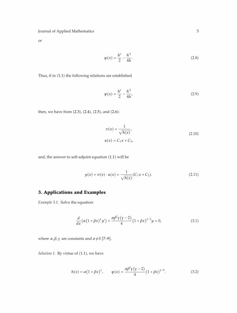
Journal of Applied Mathematics 5
or
ψ(x) =h′′
2− h
′2
4h. (2.8)
Thus, if in (1.1) the following relations are established
ψ(x) =h′′
2− h
′2
4h, (2.9)
then, we have from (2.3), (2.4), (2.5), and (2.6):
v(x) =1
√h(x)
,
u(x) = C1x + C2,
(2.10)
and, the answer to self-adjoint equation (1.1) will be
y(x) = v(x) · u(x) = 1√h(x)
(C1x + C2). (2.11)
3. Applications and Examples
Example 3.1. Solve the equation:
d
dx
(α(1 + βx
)γy′) +
αβ2γ(γ − 2
)
4(1 + βx
)γ−2y = 0, (3.1)
where α, β, γ are constants and α/= 0 [7–9].
Solution 1. By virtue of (1.1), we have
h(x) = α(1 + βx
)γ, ψ(x) =
αβ2γ(γ − 2
)
4(1 + βx
)γ−2. (3.2)

6 Journal of Applied Mathematics
Obviously, that (2.9) is established, so we have:
y(x) = v(x) · u(x) = 1√α(1 + βx
)γ(C1x + C2). (3.3)
Example 3.2. Solve the equation:
d
dx
(αeγxy′) +
αγ2
4eγxy = 0, (3.4)
where α, γ are constants and α/= 0 [7–9].
Solution 2. By virtue of (1.1), we have
h(x) = α · eγx, ψ(x) =αγ2
4eγx. (3.5)
Obviously, that (2.9) is established, so we have:
y(x) = v(x) · u(x) = 1√αeγx
(C1x + C2). (3.6)
Example 3.3. Solve the equation:
d
dx
(α · xny′) +
α · n · (n − 2)4
xn−2y = 0, (3.7)
where α, n are constants and α/= 0 [7–9].
Solution 3. By virtue of (1.1), (2.9), and (2.11), we have
y(x) = v(x) · u(x) = 1√α · xn
(C1x + C2). (3.8)
4. Conclusion
The governing equation for stability analysis of a variable cross-section bar subject to variablydistributed axial loads, dynamic analysis of multi-storey building, tall building, and othersystems is written in the form of a unified self-adjoint equation of the second order. These arereduced to Bessel’s equation in this paper.
The key step in transforming the unified equation to self-adjoint equation is theselection of h(x) and ψ(x) in (1.1).
Many difficult problems in the field of static and dynamic mechanics are solved by theunified equation proposed in this paper.

Journal of Applied Mathematics 7
References
[1] S. T. Mohyud-Din, “Solutions of nonlinear differential equations by exp-function method,” WorldApplied Sciences Journal, vol. 7, pp. 116–147, 2009.
[2] M. Allame and N. Azad, “Solution of third order nonlinear equation by Taylor Series Expansion,”World Applied Sciences Journal, vol. 14, no. 1, pp. 59–62, 2011.
[3] A. Borhanifar, M. M. Kabir, and A. HosseinPour, “A numerical method for solution of the heatequation with nonlocal nonlinear condition,” World Applied Sciences Journal, vol. 13, no. 11, pp. 2405–2409, 2011.
[4] N. H. Sweilam and A. M. Nagy, “Numerical solution of fractional wave equation using Crank-Nicholson method,” World Applied Sciences Journal, vol. 13, pp. 71–75, 2011.
[5] M. Gulsu, Y. Ozturk, and M. Sezer, “Numerical solution of singular integra-differential equationswith Cauchy Kernel,” World Applied Sciences Journal, vol. 13, no. 12, pp. 2420–2427, 2011.
[6] T. Mohyud-Din, A. Yildirim, M. Berberler, and M. Hosseini, “Numerical solution of modified equalwidth wave equation,” World Applied Sciences Journal, vol. 8, no. 7, pp. 792–798, 2010.
[7] Q. Li, H. Cao, and G. Li, “Static and dynamic analysis of straight bars with variable cross-section,”Computers and Structures, vol. 59, no. 6, pp. 1185–1191, 1996.
[8] Q. Li, H. Cao, and G. Li, “Analysis of free vibrations of tall buildings,” Journal of EngineeringMechanics,vol. 120, no. 9, pp. 1861–1876, 1994.
[9] D. Demir, N. Bildik, A. Konuralp, and A. Demir, “The numerical solutions for the damped generalizedregularized long-wave equation by variational method,” World Applied Sciences Journal, vol. 13, pp. 8–17, 2011.
[10] G. Arfken, “Self-adjoint differential equations,” in Mathematical Methods for Physicists, pp. 497–509,Academic Press, Orlando, Fla, USA, 3rd edition, 1985.
[11] M. L. Gandarias, “Weak self-adjoint differential equations,” Journal of Physics A, vol. 44, no. 26, ArticleID 262001, 2011.
[12] S. H. Javadpour, An Introduction to Ordinary and Partial Differential Equations, Alavi, Iran, 1993.[13] M. Delkhosh, “The conversion a Bessel’s equation to a self-adjoint equation and applications,” World
Applied Sciences Journal, vol. 15, no. 12, pp. 1687–1691, 2011.[14] F. B. Hilderbrand, Advanced Calculus for Applications, Prentice-Hall, 2nd edition, 1976.

Hindawi Publishing CorporationJournal of Applied MathematicsVolume 2012, Article ID 580158, 18 pagesdoi:10.1155/2012/580158
Research ArticleAlgorithms for a System of General VariationalInequalities in Banach Spaces
Jin-Hua Zhu,1 Shih-Sen Chang,2 and Min Liu1
1 Department of Mathematics, Yibin University, Sichuan, Yibin 644007, China2 College of Statistics and Mathematics, Yunnan University of Finance and Economics, Yunnan,Kunming 650221, China
Correspondence should be addressed to Shih-Sen Chang, [email protected]
Received 21 December 2011; Accepted 6 February 2012
Academic Editor: Zhenyu Huang
Copyright q 2012 Jin-Hua Zhu et al. This is an open access article distributed under the CreativeCommons Attribution License, which permits unrestricted use, distribution, and reproduction inany medium, provided the original work is properly cited.
The purpose of this paper is using Korpelevich’s extragradient method to study the existenceproblem of solutions and approximation solvability problem for a class of systems of finitefamily of general nonlinear variational inequality in Banach spaces, which includes many kindsof variational inequality problems as special cases. Under suitable conditions, some existencetheorems and approximation solvability theorems are proved. The results presented in the paperimprove and extend some recent results.
1. Introduction
Throughout this paper, we denote by N and R the sets of positive integers and real numbers,respectively. We also assume that E is a real Banach space, E∗ is the dual space of E, C is anonempty closed convex subset of E, and 〈·, ·〉 is the pairing between E and E∗.
In this paper, we are concerned a finite family of a general system of nonlinearvariational inequalities in Banach spaces, which involves finding (x∗
1, x∗2, . . . , x
∗n) ∈ C × C ×
· · · × C such that⟨λ1A1x
∗2 + x∗
1 − x∗2, j
(x − x∗
1
)⟩ ≥ 0, ∀x ∈ C,
⟨λ2A2x
∗3 + x∗
2 − x∗3, j
(x − x∗
2)⟩ ≥ 0, ∀x ∈ C,
⟨λ3A3x
∗4 + x∗
3 − x∗4, j
(x − x∗
3)⟩ ≥ 0, ∀x ∈ C,
...⟨λN−1AN−1x
∗N + x∗
N−1 − x∗N, j
(x − x∗
N−1
)⟩ ≥ 0, ∀x ∈ C,
⟨λNANx∗
1 + x∗N − x∗
1, j(x − x∗
N
)⟩ ≥ 0, ∀x ∈ C,
(1.1)

2 Journal of Applied Mathematics
where {Ai : C → E, i = 1, 2, . . . ,N} is a finite family of nonlinear mappings and λi (i = 1,2, . . . ,N) are positive real numbers.
As special cases of the problem (1.1), we have the following.(I) If E is a real Hilbert space and N = 2, then (1.1) reduces to
⟨λ1A1x
∗2 + x∗
1 − x∗2, x − x∗
1
⟩ ≥ 0, ∀x ∈ C,
⟨λ2A2x
∗1 + x∗
2 − x∗1, x − x∗
2⟩ ≥ 0, ∀x ∈ C,
(1.2)
which was considered by Ceng et al. [1]. In particular, if A1 = A2 = A, then the problem (1.2)reduces to finding (x∗
1, x∗2) ∈ C × C such that
⟨λ1Ax∗
2 + x∗1 − x∗
2, x − x∗1
⟩ ≥ 0, ∀x ∈ C,
⟨λ2Ax∗
1 + x∗2 − x∗
1, x − x∗2⟩ ≥ 0, ∀x ∈ C,
(1.3)
which is defined by Verma [2]. Furthermore, if x∗1 = x∗
2, then (1.3) reduces to the followingvariational inequality (VI) of finding x∗ ∈ C such that
〈Ax∗, x − x∗〉 ≥ 0, ∀x ∈ C. (1.4)
This problem is a fundamental problem in variational analysis and, in particular, inoptimization theory. Many algorithms for solving this problem are projection algorithmsthat employ projections onto the feasible set C of the VI or onto some related set, in orderto iteratively reach a solution. In particular, Korpelevich’s extragradient method which wasintroduced by Korpelevich [3] in 1976 generates a sequence {xn} via the recursion
yn = PC[xn − λAxn],
xn+1 = PC
[xn − λAyn
], n ≥ 0,
(1.5)
where PC is the metric projection from Rn onto C, A : C → H is a monotone operator, and λ
is a constant. Korpelevich [3] proved that the sequence {xn} converges strongly to a solutionof V I(C,A). Note that the setting of the space is Euclid space R
n.The literature on the VI is vast, and Korpelevich’s extragradient method has received
great attention by many authors, who improved it in various ways. See, for example, [4–16]and references therein.
(II) If E is still a real Banach space and N = 1, then the problem (1.1) reduces to findingx∗ ∈ C such that
⟨Ax∗, j(x − x∗)
⟩ ≥ 0, ∀x ∈ C, (1.6)
which was considered by Aoyama et al. [17]. Note that this problem is connected with thefixed point problem for nonlinear mapping, the problem of finding a zero point of a nonlinearoperator, and so on. It is clear that problem (1.6) extends problem (1.4) from Hilbert spacesto Banach spaces.

Journal of Applied Mathematics 3
In order to find a solution for problem (1.6), Aoyama et al. [17] introduced thefollowing iterative scheme for an accretive operator A in a Banach space E:
xn+1 = αnxn + (1 − αn)ΠC(xn − λnAxn), n ≥ 1, (1.7)
where ΠC is a sunny nonexpansive retraction from E to C. Then they proved a weak conver-gence theorem in a Banach space. For related works, please see [18] and the references therein.
It is an interesting problem of constructing some algorithms with strong convergencefor solving problem (1.1) which contains problem (1.6) as a special case.
Our aim in this paper is to construct two algorithms for solving problem (1.1). For thispurpose, we first prove that the system of variational inequalities (1.1) is equivalent to a fixedpoint problem of some nonexpansive mapping. Finally, we prove the strong convergence ofthe proposed methods which solve problem (1.1).
2. Preliminaries
In the sequel, we denote the strong convergence and weak convergence of the sequence {xn}by xn → x and xn ⇀ x, respectively.
For q > 1, the generalized duality mapping Jq : E → 2E∗
is defined by
Jq(x) ={f ∈ E∗ :
⟨x, f
⟩= ‖x‖q, ∥∥f∥∥ = ‖x‖q−1
}(2.1)
for all x ∈ E. In particular, J = J2 is called the normalized duality mapping. It is known thatJq(x) = ||x||q−2 for all x ∈ E. If E is a Hilbert space, then J = I, the identity mapping. LetU = {x ∈ E : ||x|| = 1}. A Banach space E is said to be uniformly convex if, for any ε ∈ (0, 2],there exists δ > 0 such that, for any x, y ∈ U,
∥∥x − y∥∥ ≥ ε implies
∥∥∥∥x + y
2
∥∥∥∥ ≤ 1 − δ. (2.2)
It is known that a uniformly convex Banach space is reflexive and strictly convex. ABanach space E is said to be smooth if the limit
limn→ 0
∥∥x + ty∥∥ − ‖x‖t
(2.3)
exists for all x, y ∈ U. It is also said to be uniformly smooth if the previous limit is attaineduniformly for x, y ∈ U. The norm of E is said to be Frechet differentiable if, for each x ∈ U,the previous limit is attained uniformly for all y ∈ U. The modulus of smoothness of E isdefined by
ρ(τ) = sup{
12(∥∥x + y
∥∥ +∥∥x − y
∥∥) − 1 : x, y ∈ E, ‖x‖ = 1,∥∥y
∥∥ = τ
}, (2.4)
where ρ : [0,∞) → [0,∞) is function. It is known that E is uniformly smooth if and only iflimτ → 0(ρ(τ)/τ) = 0. Let q be a fixed real number with 1 < q ≤ 2. Then a Banach space E is

4 Journal of Applied Mathematics
said to be q-uniformly smooth if there exists a constant c > 0 such that ρ(τ) ≤ cτq for all τ > 0.Note the following.
(1) E is a uniformly smooth Banach space if and only if J is single valued and uniformlycontinuous on any bounded subset of E.
(2) All Hilbert spaces, Lp (or lp) spaces (p ≥ 2) and the Sobolev spaces Wpm(p ≥ 2) are
2-uniformly smooth, while Lp (or lp) and WPm spaces (1 < p ≤ 2) are p-uniformly
smooth.
(3) Typical examples of both uniformly convex and uniformly smooth Banach spacesare Lp, where p > 1. More precisely, Lp is min{p, 2}-uniformly smooth for everyp > 1.
In our paper, we focus on a 2-uniformly smooth Banach space with the smooth con-stant K.
Let E be a real Banach space, C a nonempty closed convex subset of E, T : C → C amapping, and F(T) the set of fixed points of T .
Recall that a mapping T : C → C is called nonexpansive if
∥∥Tx − Ty∥∥ ≤ ∥∥x − y
∥∥, ∀x, y ∈ C. (2.5)
A bounded linear operator F : C ∈ E is called strongly positive if there exists a constant γ > 0with the property
⟨F(x), j(x)
⟩ ≥ γ‖x‖2, ∀x ∈ C. (2.6)
A mapping A : C → E is said to be accretive if there exists j(x − y) ∈ J(x − y) such that
⟨Ax −Ay, j
(x − y
)⟩ ≥ 0, (2.7)
for all x, y ∈ C, where J is the duality mapping.A mapping A of C into E is said to be α-strongly accretive if, for α > 0,
⟨Ax −Ay, j
(x − y
)⟩ ≥ α∥∥x − y
∥∥2, (2.8)
for all x, y ∈ C.A mapping A of C into E is said to be α-inverse-strongly accretive if, for α > 0,
⟨Ax −Ay, j
(x − y
)⟩ ≥ α∥∥Ax −Ay
∥∥2, (2.9)
for all x, y ∈ C.
Remark 2.1. Evidently, the definition of the inverse strongly accretive mapping is based onthat of the inverse strongly monotone mapping, which was studied by so many authors; see,for instance, [6, 19, 20].

Journal of Applied Mathematics 5
Let D be a subset of C, and let Π be a mapping of C into D. Then Π is said to besunny if
Π[Π(x) + t(x −Π(x))] = Π(x) (2.10)
whenever Π(x) + t(x −Π(x)) ∈ C for x ∈ C and t ≥ 0. A mapping Π of C into itself is calleda retraction if Π2 = Π. If a mapping Π of C into itself is a retraction, then Π(z) = z for everyz ∈ R(Π), where R(Π) is the range of Π. A subset D of C is called a sunny nonexpansiveretract of C if there exists a sunny nonexpansive retraction from C onto D. Then followinglemma concerns the sunny nonexpansive retraction.
Lemma 2.2 (see [21]). Let C be a closed convex subset of a smooth Banach space E, let D be anonempty subset of C, and letΠ be a retraction from C ontoD. ThenΠ is sunny and nonexpansive ifand only if
⟨u −Π(u), j
(y −Π(u)
)⟩ ≤ 0, (2.11)
for all u ∈ C and y ∈ D.
Remark 2.3. (1) It is well known that if E is a Hilbert space, then a sunny nonexpansive retrac-tion ΠC is coincident with the metric projection from E onto C.
(2) Let C be a nonempty closed convex subset of a uniformly convex and uniformlysmooth Banach space E, and let T be a nonexpansive mapping of C into itself with the setF(T)/= ∅. Then the set F(T) is a sunny nonexpansive retract of C.
In what follows, we need the following lemmas for proof of our main results.
Lemma 2.4 (see [22]). Assume that {αn} is a sequence of nonnegative real numbers such that
αn+1 ≤ (1 − γn
)αn + δn, (2.12)
where {γn} is a sequence in (0, 1) and {δn} is a sequence such that(a) Σ∞
n=1γn = ∞,
(b) lim supn→∞(δn/γn) ≤ 0 or Σ∞n=1|δn| < ∞.
Then limn→∞αn = 0.
Lemma 2.5 (see [23]). Let X be a Banach space, {xn}, {yn} be two bounded sequences in X and{βn} be a sequence in [0, 1] satisfying
0 < lim infn→∞
βn ≤ lim supn→∞
βn < 1. (2.13)
Suppose that xn+1 = βnxn + (1 − βn)yn, for all n ≥ 1 and
lim supn→∞
{∥∥yn+1 − yn
∥∥ − ‖xn+1 − xn‖} ≤ 0, (2.14)
then limn→∞‖yn − xn‖ = 0.

6 Journal of Applied Mathematics
Lemma 2.6 (see [24]). Let E be a real 2-uniformly smooth Banach space with the best smoothconstant K. Then the following inequality holds:
∥∥x + y
∥∥2 ≤ ‖x‖2 + 2
⟨y, Jx
⟩+ 2
∥∥Ky
∥∥2
, ∀x, y ∈ E. (2.15)
Lemma 2.7 (see [25]). Let C be a nonempty bounded closed convex subset of a uniformly convexBanach space E, and let G be a nonexpansive mapping of C into itself. If {xn} is a sequence of C suchthat xn ⇀ x and xn −Gxn → 0, then x is a fixed point of G.
Lemma 2.8 (see [26]). Let C be a nonempty closed convex subset of a real Banach space E. Assumethat the mapping F : C → E is accretive and weakly continuous along segments (i.e., F(x + ty) ⇀F(x) as t → 0). Then the variational inequality
x∗ ∈ C,⟨Fx∗, j(x − x∗)
⟩ ≥ 0, x ∈ C, (2.16)
is equivalent to the dual variational inequality
x∗ ∈ C,⟨Fx, j(x − x∗)
⟩ ≥ 0, x ∈ C. (2.17)
Lemma 2.9. Let C be a nonempty closed convex subset of a real 2-uniformly smooth Banach space E.Let ΠC be a sunny nonexpansive retraction from E onto C. Let {Ai : C → E, i = 1, 2, . . . ,N} bea finite family of γi-inverse-strongly accretive. For given (x∗
1, x∗2, . . . , x
∗n) ∈ C × C × · · · × C, where
x∗ = x∗1, x
∗i = ΠC(I−λiAi)x∗
i+1, i ∈ {i, 2, . . . ,N−1}, x∗N = ΠC(I−λNAN)x∗
1, then (x∗1, x
∗2, . . . , x
∗n)
is a solution of the problem (1.1) if and only if x∗ is a fixed point of the mapping Q defined by
Q(x) = ΠC(I − λ1A1)ΠC(I − λ2A2) · · ·ΠC(I − λNAN)(x), (2.18)
where λi (i = 1, 2, . . . ,N) are real numbers.
Proof. We can rewrite (1.1) as
⟨x∗
1 −(x∗
2 − λ1A1x∗2), j(x − x∗
1
)⟩ ≥ 0, ∀x ∈ C,
〈x∗2 −
(x∗
3 − λ2A2x∗3), j(x − x∗
2)〉 ≥ 0, ∀x ∈ C,
⟨x∗
3 −(x∗
4 − λ3A3x∗4
), j(x − x∗
3)⟩ ≥ 0, ∀x ∈ C,
...⟨x∗N−1 −
(x∗N − λN−1AN−1x
∗N
), j(x − x∗
N−1
)⟩ ≥ 0, ∀x ∈ C,
⟨x∗N − (
x∗1 − λNANx∗
1
), j(x − x∗
N
)⟩ ≥ 0, ∀x ∈ C.
(2.19)

Journal of Applied Mathematics 7
By Lemma 2.2, we can check (2.19) is equivalent to
x∗1 = ΠC(I − λ1A1)x∗
2,
x∗2 = ΠC(I − λ2A2)x∗
3,
...
x∗N−1 = ΠC(I − λN−1AN−1)x∗
N,
x∗N = ΠC(I − λNAN)x∗
1.
⇐⇒Q(x∗) = ΠC(I − λ1A1)ΠC(I − λ2A2) · · ·ΠC(I − λNAN)(x∗) = x∗.
(2.20)
This completes the proof.
Throughout this paper, the set of fixed points of the mapping Q is denoted by Ω.
Lemma 2.10. Let C be a nonempty closed convex subset of a real 2-uniformly smooth Banach spaceE. Let ΠC be a sunny nonexpansive retraction from E onto C. Let {Ai : C → E, i = 1, 2, . . . ,N} bea finite family of γi-inverse-strongly accretive. LetQ be defined as Lemma 2.9. If 0 ≤ λi ≤ γi/K
2, thenQ : C → C is nonexpansive.
Proof. First, we show that for all i ∈ {i, 2, . . . ,N}, the mapping ΠC(I − λiAi) is nonexpansive.Indeed, for all x, y ∈ C, from the condition λi ∈ [0, γi/K2] and Lemma 2.6, we have
∥∥ΠC(I − λiAi)x −ΠC(I − λiAi)y∥∥2≤ ∥∥(I − λiAi)x − (I − λiAi)y
∥∥2
=∥∥(x − y
) − λi(Aix −Aiy
)∥∥2
≤ ∥∥x − y∥∥2 − 2λi
⟨Aix −Aiy, j
(x − y
)⟩
+ 2K2λ2i
∥∥Aix −Aiy∥∥2
≤ ∥∥x − y∥∥2 − 2λiγi
∥∥Aix −Aiy∥∥2 + 2K2λ2
i
∥∥Aix −Aiy∥∥2
=∥∥x − y
∥∥2 + 2λi(K2λi − γi
)∥∥Aix −Aiy∥∥2
≤ ∥∥x − y∥∥2
,
(2.21)
which implies for all i ∈ {1, 2, . . . ,N}, the mapping ΠC(I − λiAi) is nonexpansive, so is themapping Q.

8 Journal of Applied Mathematics
3. Main Results
In this section, we introduce our algorithms and show the strong convergence theorems.
Algorithm 3.1. Let C be a nonempty closed convex subset of a uniformly convex and 2-uniformly smooth Banach space E. Let ΠC be a sunny nonexpansive retraction from E toC. Let {Ai : C → E, i = 1, 2, . . . ,N} be a finite family of γi-inverse-strongly accretive.Let B : C → E be a strongly positive bounded linear operator with coefficient α > 0 andF : C → E be a strongly positive bounded linear operator with coefficient ρ ∈ (0, α). For anyt ∈ (0, 1), define a net {xt} as follows:
xt = ΠC(tF + (I − tB))yt,
yt = ΠC(I − λ1A1)ΠC(I − λ2A2) · · ·ΠC(I − λNAN)xt,(3.1)
where, for any i, λi ∈ (0, γi/K2) is a real number.
Remark 3.2. We notice that the net {xt} defined by (3.1) is well defined. In fact, we can definea self-mapping Wt : C → C as follows:
Wtx := ΠC(tF + (I − tB))ΠC(I − λ1A1)ΠC(I − λ2A2) · · ·ΠC(I − λNAN)x, ∀x ∈ C. (3.2)
From Lemma 2.10, we know that if, for any i, λi ∈ (0, γi/K2), the mapping ΠC(I −λ1A1)ΠC(I −λ2A2) · · ·ΠC(I −λNAN) = Q is nonexpansive and ||I − tB|| ≤ 1− tα. Then, for anyx, y ∈ C, we have
∥∥Wtx −Wty∥∥ =
∥∥ΠC(tF + (I − tB))Q(x) −ΠC(tF + (I − tB))Q(y)∥∥
≤ ∥∥((tF + (I − tB))Q)x − ((tF + (I − tB))Q)y∥∥
=∥∥t(Fx − Fy
)+ (I − tB)
(Qx −Qy
)∥∥
≤ tρ∥∥x − y
∥∥ + ‖I − tB‖∥∥Qx −Qy∥∥
≤ tρ∥∥x − y
∥∥ + (1 − tα)∥∥x − y
∥∥
=(1 − (
α − ρ)t)∥∥x − y
∥∥.
(3.3)
This shows that the mapping Wt is contraction. By Banach contractive mapping principle, weimmediately deduce that the net (3.1) is well defined.
Theorem 3.3. Let C be a nonempty closed convex subset of a uniformly convex and 2-uniformlysmooth Banach space E. Let ΠC be a sunny nonexpansive retraction from E to C. Let {Ai : C →E, i = 1, 2, . . . ,N} be a finite family of γi-inverse-strongly accretive. Let B : C → E be a stronglypositive bounded linear operator with coefficient α > 0, and let F : C → E be a strongly positivebounded linear operator with coefficient ρ ∈ (0, α). Assume that Ω/= ∅ and λi ∈ (0, γi/K
2). Then the

Journal of Applied Mathematics 9
net {xt} generated by the implicit method (3.1) converges in norm, as t → 0+ to the unique solutionx of VI
x ∈ Ω,⟨(B − F)x, j(z − x)
⟩ ≥ 0, z ∈ Ω. (3.4)
Proof. We divide the proof of Theorem 3.3 into four steps.
(I) Next we prove that the net {xt} is bounded.
Take that x∗ ∈ Ω, we have
‖xt − x∗‖ =∥∥ΠC(tF + (I − tB))yt − x∗∥∥
=∥∥ΠC(tF + (I − tB))yt −ΠCx
∗∥∥
≤ ∥∥(tF + (I − tB))yt − x∗∥∥
=∥∥t(F(yt
) − F(x∗))+ (I − tB)
(yt − x∗) + tF(x∗) − tB(x∗)
∥∥
≤ t∥∥F
(yt
) − F(x∗)∥∥ + ‖I − tB‖∥∥yt − x∗∥∥ + t‖F(x∗) − B(x∗)‖
≤ tρ∥∥yt − x∗∥∥ + (1 − tα)
∥∥yt − x∗∥∥ + t‖F(x∗) − B(x∗)‖=(1 − (
α − ρ)t)∥∥yt − x∗∥∥ + t‖F(x∗) − B(x∗)‖
=(1 − (
α − ρ)t)‖Q(xt) −Q(x∗)‖ + t‖F(x∗) − B(x∗)‖
≤ (1 − (
α − ρ)t)‖xt − x∗‖ + t‖F(x∗) − B(x∗)‖.
(3.5)
It follows that
‖xt − x∗‖ ≤ ‖F(x∗) − B(x∗)‖α − ρ
. (3.6)
Therefore, {xt} is bounded. Hence, {yt}, {Byt}, {Aixt}, and {F(yt)} are also bounded. Weobserve that
∥∥xt − yt
∥∥ =∥∥ΠC(tF + (I − tB))yt −ΠCyt
∥∥
≤ ∥∥(tF + (I − tB))yt − yt
∥∥
= t∥∥F
(yt
) − B(yt
)∥∥
−→ 0.
(3.7)
From Lemma 2.10, we know that Q : C → C is nonexpansive. Thus, we have
∥∥yt −Q(yt
)∥∥ =∥∥Q(xt) −Q
(yt
)∥∥ ≤ ∥∥xt − yt
∥∥ −→ 0. (3.8)

10 Journal of Applied Mathematics
Therefore,
limt→ 0
‖xt −Q(xt)‖ = 0. (3.9)
(II) {xt} is relatively norm-compact as t → 0+.Let {tn} ⊂ (0, 1) be any subsequence such that tn → 0+ as n → ∞. Then, there exists
a positive integer n0 such that 0 < tn < 1/2, for all n ≥ n0. Let xn := xtn . It follows from (3.9)that
‖xn −Q(xn)‖ −→ 0. (3.10)
We can rewrite (3.1) as
xt = ΠC(tF + (I − tB))yt − (tF + (I − tB))yt + (tF + (I − tB))yt. (3.11)
For any x∗ ∈ Ω ⊂ C, by Lemma 2.2, we have
⟨(tF + (I − tB))yt − xt, j(x∗ − xt)
⟩
=⟨(tF + (I − tB))yt −ΠC(tF + (I − tB))yt, j
(x∗ −ΠC(tF + (I − tB))yt
)⟩ ≤ 0.(3.12)
With this fact, we derive that
‖xt − x∗‖2 =⟨x∗ − xt, j(x∗ − xt)
⟩
=⟨x∗ − (tF + (I − tB))yt, j(x∗ − xt)
⟩
+⟨(tF + (I − tB))yt −ΠC(tF + (I − tB))yt, j(x∗ − xt)
⟩
≤ ⟨(tF + (I − tB))
(x∗ − yt
), j(x∗ − xt)
⟩+ t
⟨B(x∗) − F(x∗), j(x∗ − xt)
⟩
≤ (1 − t
(α − ρ
))∥∥x∗ − yt
∥∥‖x∗ − xt‖ + t⟨B(x∗) − F(x∗), j(x∗ − xt)
⟩
=(1 − t
(α − ρ
))‖Q(x∗) −Q(xt)‖‖x∗ − xt‖ + t⟨B(x∗) − F(x∗), j(x∗ − xt)
⟩
≤ (1 − t
(α − ρ
))‖x∗ − xt‖‖x∗ − xt‖ + t⟨B(x∗) − F(x∗), j(x∗ − xt)
⟩
≤ (1 − t
(α − ρ
))‖x∗ − xt‖2 + t⟨B(x∗) − F(x∗), j(x∗ − xt)
⟩.
(3.13)
It turns out that
‖xt − x∗‖2 ≤ 1α − ρ
⟨B(x∗) − F(x∗), j(x∗ − xt)
⟩, x∗ ∈ Ω. (3.14)
In particular,
‖xn − x∗‖2 ≤ 1α − ρ
⟨B(x∗) − F(x∗), j(x∗ − xn)
⟩, x∗ ∈ Ω. (∗∗)

Journal of Applied Mathematics 11
Since {xn} is bounded, without loss of generality, xn ⇀ x ∈ C can be assumed.Noticing (3.10), we can use Lemma 2.7 to get x ∈ Ω = F(Q). Therefore, we can substitutex for x∗ in (∗∗) to get
‖xn − x‖2 ≤ 1α − ρ
⟨B(x) − F(x), j(x − xn)
⟩. (3.15)
Consequently, the weak convergence of {xn} to x actually implies that xn → x strongly. Thishas proved the relative norm compactness of the net {xt} as t → 0+.
(III) Now, we prove that x solves the variational inequality (3.4). From (3.1), we have
xt = ΠC(tF + (I − tB))yt − (tF + (I − tB))yt + (tF + (I − tB))yt
=⇒ xt = ΠC(tF + (I − tB))yt − (tF + (I − tB))yt − (tF + (I − tB))(xt − yt
)
+ tF(xt) + (I − tB)(xt)
=⇒ F(xt) − B(xt) =1t
[(tF + (I − tB))yt −ΠC(tF + (I − tB))yt − (tF + (I − tB))
(yt − xt
)].
(3.16)
For any z ∈ Ω, we obtain
⟨F(xt) − B(xt), j(z − xt)
⟩=
1t
⟨(tF + (I − tB))yt −ΠC(tF + (I − tB))yt, j(z − xt)
⟩
− 1t
⟨(tF + (I − tB))
(yt − xt
), j(z − xt)
⟩
≤ −1t
⟨(tF + (I − tB))
(yt − xt
), j(z − xt)
⟩
= −1t
⟨yt − xt, j(z − xt)
⟩+⟨(B − F)
(yt − xt
), j(z − xt)
⟩.
(3.17)
Now we prove that 〈yt −xt, j(z−xt)〉 ≥ 0. In fact, we can write yt = Q(xt). At the sametime, we note that z = Q(z), so
⟨yt − xt, j(z − xt)
⟩=⟨z −Q(z) − (xt −Q(xt)), j(z − xt)
⟩. (3.18)
Since I −Q is accretive (this is due to the nonexpansivity of Q), we can deduce immediatelythat
⟨yt − xt, j(z − xt)
⟩= 〈z −Q(z) − (
xt −Q(xt), j(z − xt)⟩ ≥ 0. (3.19)
Therefore,
⟨F(xt) − B(xt), j(z − xt)
⟩ ≤ ⟨(B − F)
(yt − xt
), j(z − xt)
⟩. (3.20)

12 Journal of Applied Mathematics
Since B, F is strongly positive, we have
0 ≤ (α − ρ
)‖z − xt‖2 ≤ ⟨(B − F)(z − xt), j(z − xt)
⟩
=⟨(F(xt) − B(xt)) − (F(z) − B(z)), j(z − xt)
⟩.
(3.21)
It follows that
⟨F(z) − B(z), j(z − xt)
⟩ ≤ ⟨F(xt) − B(xt), j(z − xt)
⟩. (3.22)
Combining (3.20) and (3.22), we get
⟨F(z) − B(z), j(z − xt)
⟩ ≤ ⟨(B − F)
(yt − xt
), j(z − xt)
⟩. (3.23)
Now replacing t in (3.23) with tn and letting n → ∞, noticing that xtn − ytn → 0, we obtain
⟨F(z) − B(z), j(z − x)
⟩ ≤ 0, z ∈ Ω, (3.24)
which is equivalent to its dual variational inequality (see Lemma 2.8)
⟨(B − F)x, j(z − x)
⟩ ≥ 0, z ∈ Ω, (3.25)
that is, x ∈ Ω is a solution of (3.4).(IV) Now we show that the solution set of (3.4) is singleton.As a matter of fact, we assume that x∗ ∈ Ω is also a solution of (3.4) Then, we have
⟨(B − F)x∗, j(x − x∗)
⟩ ≥ 0. (3.26)
From (3.25), we have
⟨(B − F)x, j(x∗ − x)
⟩ ≥ 0. (3.27)
So,
⟨(B − F)x∗, j(x − x∗)
⟩+⟨(B − F)x, j(x∗ − x)
⟩ ≥ 0
=⇒ ⟨(B − F)(x − x∗), j(x∗ − x)
⟩ ≥ 0
=⇒ ⟨(B − F)(x∗ − x), j(x∗ − x)
⟩ ≤ 0
=⇒ (α − ρ
)‖x∗ − x‖2 ≤ 0.
(3.28)
Therefore, x∗ = x. In summary, we have shown that each cluster point of {xt} (as t → 0)equals x. Therefore, xt → x as t → 0. This completes the proof.

Journal of Applied Mathematics 13
Next, we introduce our explicit method which is the discretization of the implicitmethod (3.1).
Algorithm 3.4. Let C be a nonempty closed convex subset of a uniformly convex and 2-uniformly smooth Banach space E. Let ΠC be a sunny nonexpansive retraction from E toC. Let {Ai : C → E, i = 1, 2, . . . ,N} be a finite family of γi-inverse-strongly accretive. LetB : C → E be a strongly positive bounded linear operator with coefficient α > 0, and letF : C → E be a strongly positive bounded linear operator with coefficient ρ ∈ (0, α). Forarbitrarily given x0 ∈ C, let the sequence {xn} be generated iteratively by
xn+1 = βnxn +(1 − βn
)ΠC(αnF + (I − αnB))ΠC(I − λ1A1)ΠC(I − λ2A2) · · ·ΠC(I − λNAN)xn,
n ≥ 0,(3.29)
where {αn} and {βn} are two sequences in [0, 1] and, for any i, λi ∈ (0, γi/K2) is a real number.
Theorem 3.5. Let C be a nonempty closed convex subset of a uniformly convex and 2-uniformlysmooth Banach space E, and let ΠC be a sunny nonexpansive retraction from E to C. Let {Ai : C →E, i = 1, 2, . . . ,N} be a finite family of γi-inverse-strongly accretive.Let B : C → E be a stronglypositive bounded linear operator with coefficient α > 0, and let F : C → E be a strongly positivebounded linear operator with coefficient ρ ∈ (0, α). Assume that Ω/= ∅. For given x0 ∈ C, let {xn} begenerated iteratively by (3.29). Suppose the sequences {αn} and {βn} satisfy the following conditions:
(1) limn→∞αn = 0 and Σ∞n=1αn = ∞,
(2) 0 < lim infn→∞βn ≤ lim supn→∞βn ≤ 1.
Then {xn} converges strongly to x ∈ Ω which solves the variational inequality (3.4).
Proof. Set yn = ΠC(I − λ1A1)ΠC(I − λ2A2) · · ·ΠC(I − λNAN)xn for all n ≥ 0. Then xn+1 =βnxn + (1 − βn)ΠC(αnF + (I − αnB))yn for all n ≥ 0. Pick up x∗ ∈ Ω.
From Lemma 2.10, we have
∥∥yn − x∗∥∥ = ‖Q(xn) −Q(x∗)‖ ≤ ‖xn − x∗‖. (3.30)
Hence, it follows that
‖xn+1 − x∗‖ =∥∥βnxn +
(1 − βn
)ΠC(αnF + (I − αnB))yn − x∗∥∥
=∥∥βn(xn − x∗) +
(1 − βn
)(ΠC(αnF + (I − αnB))yn − x∗)∥∥

14 Journal of Applied Mathematics
≤ βn‖xn − x∗‖ + (1 − βn
)∥∥ΠC(αnF + (I − αnB))yn −ΠCx∗∥∥
≤ βn‖xn − x∗‖ + (1 − βn
)∥∥(αnF + (I − αnB))yn − x∗∥∥
= βn‖xn − x∗‖ + (1 − βn
)∥∥(αnF + (I − αnB))(yn − x∗) + αn(F(x∗) − B(x∗))
∥∥
≤ βn‖xn − x∗‖ + (1 − βn
)(αnρ + (1 − αnα)
)∥∥yn − x∗∥∥ +(1 − βn
)αn‖F(x∗) − B(x∗)‖
≤ (1 − αn
(1 − βn
)(α − ρ
))‖xn − x∗‖ + αn
(1 − βn
)(α − ρ
)‖F(x∗) − B(x∗)‖α − ρ
.
(3.31)
By induction, we deduce that
‖xn+1 − x∗‖ ≤ max{‖x0 − x∗‖, ‖F(x
∗) − B(x∗)‖α − ρ
}. (3.32)
Therefore, {xn} is bounded. Hence, {Aixi} (i = 1, 2, . . . ,N), {yn}, {Byn}, and {F(yn)} are alsobounded. We observe that
∥∥yn+1 − yn
∥∥ = ‖Q(xn+1) −Q(xn)‖ ≤ ‖xn+1 − xn‖. (3.33)
Set xn+1 = βnxn + (1 − βn)zn for all n ≥ 0. Then zn = ΠC(αnF + (I − αnB))yn. It follows that
‖zn+1 − zn‖ =∥∥ΠC(αn+1F + (I − αn+1B))yn+1 −ΠC(αnF + (I − αnB))yn
∥∥
≤ ∥∥(αn+1F + (I − αn+1B))yn+1 − (αnF + (I − αnB))yn
∥∥
=∥∥yn+1 − yn + αn+1
(F(yn+1
) − B(yn+1
)) − αn
(F(yn
) − B(yn
))∥∥
≤ ∥∥yn+1 − yn
∥∥ + αn+1∥∥F
(yn+1
) − B(yn+1
)∥∥ − αn
∥∥F(yn
) − B(yn
)∥∥
≤ ‖xn+1 − xn‖ + αn+1∥∥F
(yn+1
) − B(yn+1
)∥∥ − αn
∥∥F(yn
) − B(yn
)∥∥.
(3.34)
This implies that
lim supn→∞
(‖zn+1 − zn‖ − ‖xn+1 − xn‖) ≤ 0. (3.35)
Hence, by Lemma 2.5, we obtain limn→∞‖zn − xn‖ = 0. Consequently,
limn→∞
‖xn+1 − xn‖ = limn→∞
(1 − βn
)‖zn − xn‖ = 0. (3.36)

Journal of Applied Mathematics 15
At the same time, we note that
∥∥zn − yn
∥∥ =
∥∥ΠC(αnF + (I − αnB))yn − yn
∥∥
=∥∥ΠC(αnF + (I − αnB))yn −ΠCyn
∥∥
≤ ∥∥(αnF + (I − αnB))yn − yn
∥∥
= αn
∥∥F
(yn
) − B(yn
)∥∥
−→ 0.
(3.37)
It follows that
limn→∞
∥∥xn − yn
∥∥ = 0. (3.38)
From Lemma 2.10, we know that Q : C → C is nonexpansive. Thus, we have
∥∥yn −Q(yn
)∥∥ =∥∥Q(xn) −Q
(yn
)∥∥ ≤ ∥∥xn − yn
∥∥ −→ 0. (3.39)
Thus, limn→∞‖xn −Q(xn)‖ = 0. We note that
‖zn −Q(zn)‖ ≤ ‖zn − xn‖ + ‖xn −Q(xn)‖ + ‖Q(xn) −Q(zn)‖≤ 2‖zn − xn‖ + ‖xn −Q(xn)‖= 2
∥∥ΠC(αnF + (I − αnB))yn −ΠCxn
∥∥ + ‖xn −Q(xn)‖≤ 2
(∥∥yn − xn
∥∥ + αn
∥∥F(yn
) − B(yn
)∥∥) + ‖xn −Q(xn)‖−→ 0.
(3.40)
Next, we show that
lim supn→∞
⟨F(x) − B(x), j(zn − x)
⟩ ≤ 0, (3.41)
where x ∈ Ω is the unique solution of VI(3.4).To see this, we take a subsequence {znj} of {zn} such that
limn→∞
⟨F(x) − B(x), j(zn − x)
⟩= lim
nj →∞
⟨F(x) − B(x), j
(znj − x
)⟩. (3.42)
We may also assume that znj ⇀ z. Note that z ∈ Ω in virtue of Lemma 2.7 and (3.40). Itfollows from the variational inequality (3.4) that
limn→∞
⟨F(x) − B(x), j(zn − x)
⟩= lim
nj →∞
⟨F(x) − B(x), j
(znj − x
)⟩
=⟨F(x) − B(x), j(z − x)
⟩ ≤ 0.(3.43)

16 Journal of Applied Mathematics
Since zn = ΠC(αnF + (I − αnB))yn, according to Lemma 2.2, we have
⟨(αnF + (I − αnB))yn −ΠC(αnF + (I − αnB))yn, j(x − zn)
⟩ ≤ 0. (3.44)
From (3.44), we have
‖zn − x‖2 =⟨ΠC(αnF + (I − αnB))yn − x, j(zn − x)
⟩
=⟨ΠC(αnF + (I − αnB))yn − (αnF + (I − αnB))yn, j(zn − x)
⟩
+⟨(αnF + (I − αnB))yn − x, j(zn − x)
⟩
≤ ⟨(αnF + (I − αnB))yn − x, j(zn − x)
⟩
=⟨(αnF + (I − αnB))
(yn − x
), j(zn − x)
⟩+ αn
⟨F(x) − B(x), j(zn − x)
⟩
≤ (1 − αn
(α − ρ
))∥∥yn − x∥∥‖zn − x‖ + αn
⟨F(x) − B(x), j(zn − x)
⟩
≤(1 − αn
(α − ρ
))2
2∥∥yn − x
∥∥2 +12‖zn − x‖2 + αn
⟨F(x) − B(x), j(zn − x)
⟩.
(3.45)
It follows that
‖zn − x‖2 ≤ (1 − αn
(α − ρ
))∥∥yn − x∥∥2 + 2αn
⟨F(x) − B(x), j(zn − x)
⟩,
≤ (1 − αn
(α − ρ
))‖xn − x‖2 + 2αn
⟨F(x) − B(x), j(zn − x)
⟩.
(3.46)
Finally, we prove xn → x. From xn+1 = βnxn + (1 − βn)zn and (3.46), we have
‖xn+1 − x‖2 ≤ βn‖xn − x‖2 +(1 − βn
)‖zn − x‖2
≤ βn‖xn − x‖2 +(1 − βn
)((1 − αn
(α − ρ
))‖xn − x‖2 + 2αn
⟨F(x) − B(x), j(zn − x)
⟩)
=(1 − αn
(1 − βn
)(α − ρ
))‖xn − x‖2 + αn
(1 − βn
)(α − ρ
)
×{
2α − ρ
⟨F(x) − B(x), j(zn − x)
⟩}.
(3.47)
We can apply Lemma 2.4 to the relation (3.47) and conclude that xn → x. This completes theproof.
Acknowledgments
The authors would like to express their thanks to the referees and the editor for theirhelpful suggestion and comments. This work was supported by the Scientific Reserch Fundof Sichuan Provincial Education Department (09ZB102,11ZB146) and Yunnan University ofFinance and Economics.

Journal of Applied Mathematics 17
References
[1] L.-C. Ceng, C.-y. Wang, and J.-C. Yao, “Strong convergence theorems by a relaxed extragradientmethod for a general system of variational inequalities,” Mathematical Methods of Operations Research,vol. 67, no. 3, pp. 375–390, 2008.
[2] R. U. Verma, “On a new system of nonlinear variational inequalities and associated iterativealgorithms,” Mathematical Sciences Research Hot-Line, vol. 3, no. 8, pp. 65–68, 1999.
[3] G. M. Korpelevich, “An extragradient method for finding saddle points and for other problems,”Ekonomika i Matematicheskie Metody, vol. 12, no. 4, pp. 747–756, 1976.
[4] Y. Censor, A. Gibali, and S. Reich, “Two extensions of Korplevich’s extragradient method for solvingthe variational inequality problem in Euclidean space,” Tech. Rep., 2010.
[5] L.-C. Zeng and J.-C. Yao, “Strong convergence theorem by an extragradient method for fixed pointproblems and variational inequality problems,” Taiwanese Journal of Mathematics, vol. 10, no. 5, pp.1293–1303, 2006.
[6] H. Iiduka and W. Takahashi, “Strong convergence theorems for nonexpansive mappings and inverse-strongly monotone mappings,” Nonlinear Analysis. Theory, Methods & Applications, vol. 61, no. 3, pp.341–350, 2005.
[7] N. Nadezhkina and W. Takahashi, “Weak convergence theorem by an extragradient method fornonexpansive mappings and monotone mappings,” Journal of Optimization Theory and Applications,vol. 128, no. 1, pp. 191–201, 2006.
[8] Y. Yao and M. A. Noor, “On viscosity iterative methods for variational inequalities,” Journal ofMathematical Analysis and Applications, vol. 325, no. 2, pp. 776–787, 2007.
[9] Y. Yao, M. A. Noor, R. Chen, and Y.-C. Liou, “Strong convergence of three-step relaxed hybridsteepest-descent methods for variational inequalities,” Applied Mathematics and Computation, vol. 201,no. 1-2, pp. 175–183, 2008.
[10] R. U. Verma, “Projection methods, algorithms, and a new system of nonlinear variationalinequalities,” Computers & Mathematics with Applications, vol. 41, no. 7-8, pp. 1025–1031, 2001.
[11] R. U. Verma, “General convergence analysis for two-step projection methods and applications tovariational problems,” Applied Mathematics Letters, vol. 18, no. 11, pp. 1286–1292, 2005.
[12] Y. Yao, Y.-C. Liou, and J.-C. Yao, “An extragradient method for fixed point problems and variationalinequality problems,” Journal of Inequalities and Applications, Article ID 38752, 12 pages, 2007.
[13] Y. Yao and J.-C. Yao, “On modified iterative method for nonexpansive mappings and monotonemappings,” Applied Mathematics and Computation, vol. 186, no. 2, pp. 1551–1558, 2007.
[14] Y. Censor, A. Gibali, and S. Reich, “The subgradient extragradient method for solving variationalinequalities in Hilbert space,” Journal of Optimization Theory and Applications, vol. 148, no. 2, pp. 318–335, 2011.
[15] Z. Huang and M. A. Noor, “An explicit projection method for a system of nonlinear variationalinequalities with different (γ ,r)-cocoercive mappings,” Applied Mathematics and Computation, vol. 190,no. 1, pp. 356–361, 2007.
[16] Z. Huang and M. A. Noor, “Some new unified iteration schemes with errors for nonexpansivemappings and variational inequalities,” Applied Mathematics and Computation, vol. 194, no. 1, pp. 135–142, 2007.
[17] K. Aoyama, H. Iiduka, and W. Takahashi, “Weak convergence of an iterative sequence for accretiveoperators in Banach spaces,” Fixed Point Theory and Applications, Article ID 35390, 13 pages, 2006.
[18] S. Kamimura and W. Takahashi, “Weak and strong convergence of solutions to accretive operatorinclusions and applications,” Set-Valued Analysis, vol. 8, no. 4, pp. 361–374, 2000.
[19] W. Takahashi and M. Toyoda, “Weak convergence theorems for nonexpansive mappings andmonotone mappings,” Journal of Optimization Theory and Applications, vol. 118, no. 2, pp. 417–428,2003.
[20] H. Iiduka, W. Takahashi, and M. Toyoda, “Approximation of solutions of variational inequalities formonotone mappings,” Panamerican Mathematical Journal, vol. 14, no. 2, pp. 49–61, 2004.
[21] S. Reich, “Weak convergence theorems for nonexpansive mappings in Banach spaces,” Journal ofMathematical Analysis and Applications, vol. 67, no. 2, pp. 274–276, 1979.
[22] H.-K. Xu, “Iterative algorithms for nonlinear operators,” Journal of the London Mathematical Society,vol. 66, no. 1, pp. 240–256, 2002.
[23] T. Suzuki, “Strong convergence of Krasnoselskii and Mann’s type sequences for one-parameter non-expansive semigroups without Bochner integrals,” Journal of Mathematical Analysis and Applications,vol. 305, no. 1, pp. 227–239, 2005.

18 Journal of Applied Mathematics
[24] H. K. Xu, “Inequalities in Banach spaces with applications,” Nonlinear Analysis. Theory, Methods &Applications, vol. 16, no. 12, pp. 1127–1138, 1991.
[25] K. Goebel and W. A. Kirk, “Topics in metric fixed point theory,” in Cambridge Studies in AdvancedMathematics, vol. 28, Cambridge University Press, Cambridge, UK, 1990.
[26] Y. Yao, Y.-C. Liou, S. M. Kang, and Y. Yu, “Algorithms with strong convergence for a systemof nonlinear variational inequalities in Banach spaces,” Nonlinear Analysis. Theory, Methods &Applications, vol. 74, no. 17, pp. 6024–6034, 2011.

Hindawi Publishing CorporationJournal of Applied MathematicsVolume 2012, Article ID 351764, 10 pagesdoi:10.1155/2012/351764
Research ArticleFinite Difference Method for Solving a System ofThird-Order Boundary Value Problems
Muhammad Aslam Noor,1 Eisa Al-Said,2and Khalida Inayat Noor1
1 Department of Mathematics, COMSATS Institute of Information Technology,Park Road, Chak Shahzad, Islamabad, Pakistan
2 Department of Mathematics, College of Science, King Saud University, P.O. Box 2455,Riyadh 11451, Saudi Arabia
Correspondence should be addressed to Muhammad Aslam Noor, [email protected]
Received 2 November 2011; Revised 7 February 2012; Accepted 8 February 2012
Academic Editor: Zhenyu Huang
Copyright q 2012 Muhammad Aslam Noor et al. This is an open access article distributed underthe Creative Commons Attribution License, which permits unrestricted use, distribution, andreproduction in any medium, provided the original work is properly cited.
We develop a new-two-stage finite difference method for computing approximate solutions ofa system of third-order boundary value problems associated with odd-order obstacle problems.Such problems arise in physical oceanography (Dunbar (1993) and Noor (1994), draining andcoating flow problems (E. O. Tuck (1990) and L. W. Schwartz (1990)), and can be studied in theframework of variational inequalities. We show that the present method is of order three and givenumerical results that are better than the other available results. Numerical example is presentedto illustrate the applicability and efficiency of the new method.
1. Introduction
Variational inequalities have had a great impact and influence in the development of almostall branches of pure and applied sciences. It has been shown that the variational inequalitiesprovide a novel and general framework to study a wide class of problems arising in variousbranches of pure and applied sciences. The ideas and techniques of variational inequalitiesare being used in a variety of diverse fields and proved to be innovative and productive,see [1–15] and the references therein. In recent years, variational inequalities have beenextended and generalized in several directions. A useful and important generalization ofvariational inequalities is called the general variational inequalities involving two continuousoperators, which was introduced by Noor [10] in 1988. It has been shown that a wide class ofnonsymmetric and odd-order obstacle problems arising in industry, economics, optimization,

2 Journal of Applied Mathematics
mathematical and engineering sciences can be studied in the unified and general frameworkof the general variational inequalities, see [1–5, 11–19] and the references therein. Despite oftheir importance, little attention has been given to develop some efficient numerical techniqueof solving such type of problems. In principle, the finite difference techniques and otherrelated methods cannot be applied directly to solve the obstacle-type problems. Using thetechnique of the penalty method, one rewrite the general variational inequalities as generalvariational equations. We note that, if the obstacle function is known, then one can use theidea and technique of Lewy and Stampacchia [9] to express the general variational equationsas a system of third-order boundary value problems. This resultant system of equationscan be solved, which is the main advantage of this approach. The computational aspect ofthis method is its simple applicability for solving obstacle problems. Such type of penaltyfunction method in conjunction with spline and finite difference techniques has been usedquite effectively as a basis for solving system of third-order boundary value problems, see [1–5, 7, 13, 15–17, 19]. Our approach to these problems is to consider them in a general mannerand specialize them later on. To convey an idea of the technique involved, we first introduceand develop a new two stage finite difference scheme for solving a third-order boundaryvalue problems. An example involving the order-order obstacle problem is given to illustratethe efficiency and its comparison with other methods.
For simplicity and to convey an idea of the obstacle problems, we consider a system ofthird-order boundary value problem of the type, which was first considered by Noor [11]
u′′′ =
⎧⎪⎪⎨
⎪⎪⎩
f(x), a ≤ x ≤ c,
p(x)u(x) + f(x) + r, c ≤ x ≤ d,
f(x), d ≤ x ≤ b,
(1.1a)
with the boundary conditions
u(a) = α, u′(a) = β1, u′(b) = β2, (1.1b)
and the continuity conditions of u, u′, and u′′ at c and d. Here, f and p are continuousfunctions on [a, b] and [c, d], respectively. The parameters r, α, β1, and β2 are real finiteconstants. Using the penalty method technique, one can easily show that a wide class ofunrelated obstacle, unilateral, moving and free boundary value problems arising in variousbranches of pure and applied sciences can be characterized by the system of third-orderboundary value problems of type (1.1a) and (1.1b), see, for example, [1–17] and the referencestherein. In general, it is not possible to obtain the analytical solution of (1.1a) and (1.1b) forarbitrary choices of f(x) and p(x). We usually resort to some numerical methods for obtainingan approximate solution of (1.1a) and (1.1b).
The available finite difference and collocation methods are not suitable for solvingsystem of boundary value problems of the form defined by (1.1a) and (1.1b). Such methodshave a serious drawback in the accuracy regardless of the order of the convergent of themethod being used, see [2, 4, 7, 13, 16, 17, 19]. On the other hand, Al-Said [1], Al-Said andNoor [3], Al-Said et al. [5] and Noor and Al-Said [16] have developed first- and second-order

Journal of Applied Mathematics 3
two-stage difference methods for solving (1.1a) and (1.1b), which gives numerical resultsthat better than those produced by the first-, second- and, third-order methods considered in[2, 4, 7, 13, 16, 17, 19].
Motivated by the above works, we suggest a new two-stage numerical algorithm forsolving the system of third-order boundary value problem (1.1a) and (1.1b). We prove thatthe present method is of order two, and it outperforms other collocation and finite differencemethods when solving (1.1a) and (1.1b). In Section 2, we derive the numerical method forsolving (1.1a) and (1.1b). Section 3 is devoted for the convergence analysis of the method.The numerical experiments and comparison with other methods are given in Section 4.
2. Numerical Method
For simplicity, we take c = (3a + b)/4 and d = (a + 3b)/4 in order to develop the numericalmethod for solving the system of differential equations (1.1a) and (1.1b). For this purposewe divide the interval [a, b] into n equal subintervals using the grid points xi = a + ih, i =0, 1, 2, . . . , n, x0 = a, xn = b and
h =b − a
n, (2.1)
where n is a positive integer chosen such that both n/4 and 3n/4 are also positive integers.Using Taylor series expansions along with the method of undetermined coefficients,
boundary and continuity conditions to develop the following finite difference scheme:
9u1/2 − u3/2 = 8u0 + 3hu′0 −
1160
h3[6u′′′
0 + 51u′′′1/2 + 3u′′′
3/2
]+ t1, for i = 1,
− 2u1/2 + 3u3/2 − u5/2 = +hu′0 −
11920
h3[809u′′′
1/2 + 1062u′′′3/2 − 31u′′′
5/2
]+ t2, for i = 2,
ui−5/2 − 3ui−3/2 + 3ui−1/2 − ui+1/2 =16h3[−u′′′
i−5/2 + 6u′′′i−3/2 + u′′′
i+1/2
]+ ti, for 3 ≤ i ≤ n − 1,
un−5/2 − 3un−3/2 + 2un−1/2=hu′n −
11920
h3[−31u′′′
n−5/2 + 1062u′′′n−3/2 + 809u′′′
n−1/2
]+ tn, for i = n,
(2.2)
where
u′′′i+1/2 =
⎧⎪⎪⎨
⎪⎪⎩
fi+1/2, for 0 ≤ i ≤ n
4− 1,
3n4
≤ i ≤ n − 1
pi+1/2ui+1/2 + fi+1/2 + r, forn
4≤ i ≤ 3n
4− 1,
(2.3)

4 Journal of Applied Mathematics
fi+1/2 = f(xi+1/2), i = 0, 1, 2, . . . , n−1, the relation (2.2) forms a system of n linear equations inthe unknowns ui−1/2, i = 1, 2, . . . , n. The local truncation errors associate with (2.2) are givenby
ti =
⎧⎪⎪⎪⎪⎪⎪⎪⎪⎪⎪⎪⎪⎨
⎪⎪⎪⎪⎪⎪⎪⎪⎪⎪⎪⎪⎩
49320
h6u(vi)0 +O
(h7), for i = 1,
− 533840
h6u(vi)0 +O
(h7), for i = 2,
15237680
h6u(vi)i +O
(h7), for 3 ≤ i ≤ n − 1,
− 533840
h6u(vi)i +O
(h7), for i = n,
(2.4)
which suggest that the scheme (2.2) is a third-order accurate.
Remark 2.1. The new method can be considered as an improvement of the previous finitedifference methods at the midknots developed in [1, 3, 4, 16] for solving the third-orderobstacle problem. Thus, the matrix remains the same for the sake of comparison with othermethods. We would like to point out that the same goes for the finite difference methods atthe knots for solving third-order boundary value problems, see the references.
3. Convergence Analysis
In this section, we investigate the convergence analysis of the method developed in Section 2.For this purpose, we first let u = (ui+1/2), w = (wi+1/2), c = (ci), t = (ti), and e = (ei+1/2) ben-dimensional column vectors. Here ei+1/2 = ui+1/2 − wi+1/2 is the discretization error. Thus,we can write our method as follow:
Au = c + t, (3.1a)Aw = c, (3.1b)Ae = t, (3.1c)
where
A = A0 +1
1920h3BP, (3.2)
P = diag(pi−1/2), i = 1, 2, . . . , n, with pi−1/2 /= 0 for n/4 < i ≤ 3n/4,
A0 =
⎡
⎢⎢⎢⎢⎢⎢⎢⎢⎢⎢⎢⎣
9 −1 0 · · · · · · · · · 0−2 3 −1 0 · · · · · · 01 −3 3 −1 0 · · · 0
0. . . . . . . . . . . . · · · 0
.... . . . . . . . . . . . . . .
...0 · · · 0 1 −3 3 −10 · · · · · · 0 1 −3 2
⎤
⎥⎥⎥⎥⎥⎥⎥⎥⎥⎥⎥⎦
, (3.3)

Journal of Applied Mathematics 5
and the lower triangular matrix
B =
⎡
⎢⎢⎢⎢⎢⎢⎢⎢⎢⎢⎢⎣
612 36 0 · · · · · · · · · 01062 −31 0 · · · · · · 0
0 320 0 · · · 0
0. . . . . .
. . . . . . . . . 0...
. . . . . . . . . . . . . . ....
0 · · · 0 0 3200 · · · · · · 0 809
⎤
⎥⎥⎥⎥⎥⎥⎥⎥⎥⎥⎥⎦
. (3.4)
For the vector c, we have
ci =
⎧⎪⎪⎪⎪⎪⎪⎪⎪⎪⎪⎪⎪⎪⎪⎪⎪⎪⎪⎪⎪⎪⎪⎪⎪⎪⎪⎪⎪⎪⎪⎪⎪⎪⎪⎪⎪⎪⎪⎨
⎪⎪⎪⎪⎪⎪⎪⎪⎪⎪⎪⎪⎪⎪⎪⎪⎪⎪⎪⎪⎪⎪⎪⎪⎪⎪⎪⎪⎪⎪⎪⎪⎪⎪⎪⎪⎪⎪⎩
8α + 3hβ1 − 1160
h3F1, i = 1,
hβ1 − 11920
h3F2, i = 2,
−16h3Fi, 3 ≤ i ≤ n
4− 1,
3n4
+ 3 ≤ i ≤ n − 1,
−16h3[Fi + r], i =
n
4, i =
n
4+ 1,
−16h3[Fi + 7r], i =
n
4+ 2,
−16h3[Fi + 6r],
n
4+ 3 ≤ i ≤ 3n
4− 1,
−16h3[Fi + 5r], i =
3n4, i =
3n4
+ 1,
− 112
h3[Fi − r], i =3n4
+ 2,
hβ2 − 11920
h3Fn, i = n,
(3.5)
where
Fi =
⎧⎪⎪⎪⎪⎪⎪⎪⎪⎨
⎪⎪⎪⎪⎪⎪⎪⎪⎩
51f1/2 + 3f3/2, i = 1,
809f1/2 + 1062f3/2 − 3125f5/2, i = 2,
−fi−5/2 + 8fi−3/2 + fi+1/2, 3 ≤ i ≤ n − 1,
−31fn−5/2 + 1062fn−3/2 + 908fn−1/2, i = n.
(3.6)

6 Journal of Applied Mathematics
Our main purpose now is to derive a bound on ‖e‖, where ‖ · ‖ represents the ∞-norm.It has been shown in [1] that A−1
0 exits and satisfies the equation
∥∥∥A−1
0
∥∥∥ =
4n3 − n + 348
, (3.7)
which upon using (2.1) we obtain
∥∥∥A−1
0
∥∥∥ =
3h3 − (b − a)h2 + 4(b − a)3
48h3. (3.8)
Thus, using (3.1a)–(3.1c) and (3.2) and the fact that ‖B‖ = 2560 and ‖P‖ ≤ |p(x)|, we get
‖e‖ ≤ 1523λM6h3
2560[3 − 4λ
∣∣p(x)∣∣]
∼= O(h3), (3.9)
where λ = (1/48)[h3 − (b − a)h2 + (b − a)3] and M6 = max |y(vi)(x)|, see [1] for more details.Relation (3.9) indicates that (3.1b) is a third-order convergent method.
Remark 3.1. The matrix A0 and its inverse were first introduced in [1]. The derivation of (3.7)(the elements of A−1
0 ) given in [1] was derived using the definition of the matrix inverse. Thederivation involves a long and complicated algebraic manipulations. The interested readermay try to derive it.
4. Applications and Computational Results
To illustrate the application of the numerical method developed in the previous sections, weconsider the third-order obstacle boundary value problem of finding u such that
−u′′′ ≥ f, on Ω = [0, 1],
u ≥ ψ, on Ω = [0, 1],[−u′′′ − f
][u − ψ
]= 0, on Ω = [0, 1],
u(0) = 0, u′(0) = 0, u′(1) = 0,
(4.1)
where f(x) is a continuous function and ψ(x) is the obstacle function. We study the problem(4.1) in the framework of variational inequality approach. To do so, we first define the set Kas
K ={v : v ∈ H2
0(Ω) : v ≥ ψ on Ω}, (4.2)

Journal of Applied Mathematics 7
which is a closed convex set in H20(Ω), where H2
0(Ω) is a Sobolev (Hilbert) space, see [8]. Onecan easily show that the energy functional associated with the problem (4.1) is
I[v] = −∫1
0
(d3v
dx3
)(dv
dx
)dx − 2
∫1
0f(x)
(dv
dx
)dx, ∀ dv
dx∈ K
=∫1
0
(d2v
dx2
)2
dx − 2∫1
0f(x)
(dv
dx
)dx
=⟨Tv, g(v)
⟩ − 2⟨f, g(v)
⟩,
(4.3)
⟨Tu, g(v)
⟩=∫1
0
(d2u
dx2
)(d2v
dx2
)
dx,
⟨f, g(v)
⟩=∫1
0f(x)
dv
dxdx,
(4.4)
and g = d/dx is the linear operator.It is clear that the operator T defined by (4.4) is linear, g-symmetric, and g-positive.
Using the technique of Noor [13, 15], one can easily show that the minimum u ∈ H of thefunctional I[v] defined by (4.3) associated with the problem (4.1) on the closed convex set Kcan be characterized by the inequality of the type
⟨Tu, g(v) − g(u)
⟩ ≥ ⟨f, g(v) − g(u)
⟩, ∀g(v) ∈ K, (4.5)
which is exactly the general variational inequality, considered by Noor [10] in 1988. It isworth mentioning that a wide class of unrelated odd-order and nonsymmetric equilibriumproblems arising in regional, physical, mathematical, engineering, and applied sciences canbe studied in the unified and general framework of the general variational inequalities, see[1–20].
Using the penalty function technique of Lewy and Stampacchia [9], we can character-ize the problem (4.1) as
−u′′′ + ν{(
u − ψ)}(
u − ψ)= f, 0 < x < 1,
u(0) = u′(0) = u′(1) = 0,(4.6)
where
ν{t} =
{1, for t ≥ 0,0, for t < 0
(4.7)

8 Journal of Applied Mathematics
is a discontinuous function and is known as the penalty function and ψ is the given obstaclefunction defined by
ψ(x) =
⎧⎪⎪⎨
⎪⎪⎩
−1, for 0 ≤ x ≤ 14,
34≤ x ≤ 1,
1, for14≤ x ≤ 3
4.
(4.8)
From equations (4.3)–(4.8), we obtain the following system of differential equations:
u′′′ =
⎧⎪⎪⎨
⎪⎪⎩
f, for 0 ≤ x ≤ 14,
34≤ x ≤ 1,
u + f − 1, for14≤ x ≤ 3
4,
(4.9)
with the boundary conditions
u(0) = u′(0) = u′(1) = 0 (4.10)
and the condition of continuity of u, u′ and u′′ at x = 1/4 and 3/4. Note that the system ofdifferential equations (4.7) is a special form of the system (1.1a) with p(x) = 1 and r = −1.
Example 4.1. For f = 0, the system of differential equations (4.9) reduces to
u′′′ =
⎧⎪⎪⎨
⎪⎪⎩
0, for 0 ≤ x ≤ 14,
34≤ x ≤ 1,
u − 1, for14≤ x ≤ 3
4,
(4.11)
with the boundary conditions (4.10). The analytical solution for this problem is
u(x) =
⎧⎪⎪⎪⎪⎪⎪⎪⎨
⎪⎪⎪⎪⎪⎪⎪⎩
12a1x
2, 0 ≤ x ≤ 14,
1 + a2ex + e−x/2
[
a3 cos√
32
x + a4 sin√
32
x
]
,14≤ x ≤ 3
4,
12a5x(x − 2) + a6,
34≤ x ≤ 1.
(4.12)
We can find the constants ai, i = 1, 2, . . . , 6, by solving a system of linear equations con-structed by applying the continuity conditions of u, u′, and u′′ at x = 1/4 and 3/4, see [3] formore details.
For different values of h, the boundary value problem defined by (4.10) and (4.11) wassolved using the numerical methods developed in the previous sections and the observedmaximum errors ‖e‖ are listed in Table 1. Also, we give in Table 1 the numerical results forthe finite difference methods at midkonts introduced in [1, 3, 5, 16]. It is clear from this table

Journal of Applied Mathematics 9
Table 1: Observed maximum errors ‖e‖.
h New method [1] [3] [5] [16]
1/20 4.05 ×10⁻⁵ 4.96 ×10⁻⁵ 1.48 ×10⁻⁴ 6.74 ×10⁻⁴ 1.04 ×10⁻³
1/40 9.78 ×10⁻⁶ 1.24 ×10⁻⁵ 3.70 ×10⁻⁵ 3.04 ×10⁻⁴ 2.60 ×10⁻⁴
1/80 2.31 ×10⁻⁶ 3.10 ×10⁻⁶ 9.24 ×10⁻⁶ 1.37 ×10⁻⁴ 6.49 ×10⁻⁵
Table 2: Observed maximum errors.
h New method [2] [7] [17] [19]
1/32 2.57 ×10⁻⁵ 5.53 ×10⁻⁴ 5.30 ×10⁻⁴ 5.32 ×10⁻⁴ 4.05 ×10⁻⁴
1/64 6.38 ×10⁻⁶ 2.61 ×10⁻⁴ 2.52 ×10⁻⁴ 2.56 ×10⁻⁴ 2.24 ×10⁻⁴
1/128 1.47 ×10⁻⁶ 1.27 ×10⁻⁴ 1.23 ×10⁻⁴ 1.26 ×10⁻⁴ 1.15 ×10⁻⁴
that our present method produced better results than the other ones. However, the numericalresults may indicate that we have second-order approximations. This is due to the fact thatthe third derivative is not continuous across the interfaces.
Now, let wi−1/2 be an approximate value of ui−1/2, for i = 1, 2, . . . , n, computed by thenumerical method developed in the previous sections. Then having the values of wi−1/2, fori = 1, 2, . . . , n, we can compute wi ≈ ui using the second-order interpolating
ui =12[ui+1/2 + ui−1/2] +O
(h2), (4.13)
for i = 1, 2, . . . , n. Note that we make use of the boundary condition u′(1) = 0 to computethe value of wn. The computations of wi, i = 1, 2, . . . , n, give us the opportunity for a farecomparisons with the other methods discussed in [2, 7, 17, 19], which approximate thesolution of problems (4.11) at the nodes. In Table 2, we list the maximum value for the errorsmaxi|ui −wi| for different h values for our present method and the others. From Table 2, it canbe noted that our present method gives the best results. We mentioned here in passing thatthe numerical results for the method developed in [4] are worse than those given in Table 2and are not presented here.
5. Conclusion
As mentioned in [1, 3, 5, 16] where two-stage first- and second-order method was developed,we have noticed from our experiments that the maximum value of the error occurs nearthe center of the interval and not around x = 1/4 nor 3/4, where the solution satisfies theextraconditions. On the other hand, it was noticed from the experiments done by the authorsin [2, 4, 17] that the maximum error occurs at near the indicated values of x. Thus, we canconclude that the extra conditions at x = 1/4 and 3/4 have little effect on the performance ofthe methods that first approximate the solution at the midknots, whereas for the other twomethods these added conditions introduce a serious drawback in the accuracy.

10 Journal of Applied Mathematics
Acknowledgments
This paper is supported by the Visiting Professor Program of King Saud University, Riyadh,Saudi Arabia. The authors would like to thank the referees for their valuable input andcomments.
References
[1] E. A. Al-Said, “Numerical solutions for system of third-order boundary value problems,” InternationalJournal of Computer Mathematics, vol. 78, no. 1, pp. 111–121, 2001.
[2] E. A. Al-Said and M. A. Noor, “Cubic splines method for a system of third-order boundary value prob-lems,” Applied Mathematics and Computation, vol. 142, no. 2-3, pp. 195–204, 2003.
[3] E. A. Al-Said and M. A. Noor, “Numerical solutions of third-order system of boundary value prob-lems,” Applied Mathematics and Computation, vol. 190, no. 1, pp. 332–338, 2007.
[4] E. A. Al-Said, M. A. Noor, and A. K. Khalifa, “Finite difference scheme for variational inequalities,”Journal of Optimization Theory and Applications, vol. 89, no. 2, pp. 453–459, 1996.
[5] E. A. Al-Said, M. A. Noor, and Th. M. Rassias, “Numerical solutions of third-order obstacle prob-lems,” International Journal of Computer Mathematics, vol. 69, no. 1-2, pp. 75–84, 1998.
[6] S. R. Dunbar, “Geometric analysis of a nonlinear boundary value problem from physical oceanogra-phy,” SIAM Journal on Mathematical Analysis, vol. 24, no. 2, pp. 444–465, 1993.
[7] F. Gao and C.-M. Chi, “Solving third-order obstacle problems with quartic B-splines,” Applied Mathe-matics and Computation, vol. 180, no. 1, pp. 270–274, 2006.
[8] D. Kinderlehrer and G. Stampacchia, An Introduction to Variational Inequalities and Their Applications,Society for Industrial and Applied Mathematics (SIAM), Philadelphia, Pa, USA, 2000.
[9] H. Lewy and G. Stampacchia, “On the regularity of the solution of a variational inequality,” Commu-nications on Pure and Applied Mathematics, vol. 22, pp. 153–188, 1969.
[10] M. A. Noor, “General variational inequalities,” Applied Mathematics Letters, vol. 1, no. 2, pp. 119–122,1988.
[11] M. A. Noor, “Variational inequalities in physical oceanography,” in Ocean Waves Engineering, M.Rahman, Ed., pp. 201–266, Computational Mechanics, London, UK, 1994.
[12] M. A. Noor, “New approximation schemes for general variational inequalities,” Journal of Mathemati-cal Analysis and Applications, vol. 251, no. 1, pp. 217–229, 2000.
[13] M. A. Noor, “Some recent advances in variational inequalities. I. Basic concepts,” New Zealand Journalof Mathematics, vol. 26, no. 1, pp. 53–80, 1997.
[14] M. A. Noor, “Some developments in general variational inequalities,” Applied Mathematics and Com-putation, vol. 152, no. 1, pp. 199–277, 2004.
[15] M. A. Noor, “Extended general variational inequalities,” Applied Mathematics Letters, vol. 22, no. 2, pp.182–186, 2009.
[16] M. A. Noor and E. A. Al-Said, “Finite-difference method for a system of third-order boundary-valueproblems,” Journal of Optimization Theory and Applications, vol. 112, no. 3, pp. 627–637, 2002.
[17] M. A. Noor and E. E. Al-Said, “Quartic splines solutions of third-order obstacle problems,” AppliedMathematics and Computation, vol. 153, no. 2, pp. 307–316, 2004.
[18] M. A. Noor, K. I. Noor, and T. M. Rassias, “Some aspects of variational inequalities,” Journal of Com-putational and Applied Mathematics, vol. 47, no. 3, pp. 285–312, 1993.
[19] Siraj-ul-Islam, M. A. Khan, I. A. Tirmizi, and E. H. Twizell, “Non polynomial spline approach to thesolution of a system of third-order boundary-value problems,” Applied Mathematics and Computation,vol. 168, no. 1, pp. 152–163, 2005.
[20] E. O. Tuck and L. W. Schwartz, “A numerical and asymptotic study of some third-order ordinary dif-ferential equations relevant to draining and coating flows,” SIAM Review, vol. 32, no. 3, pp. 453–469,1990.

Hindawi Publishing CorporationJournal of Applied MathematicsVolume 2012, Article ID 413468, 15 pagesdoi:10.1155/2012/413468
Research ArticleExistence and Algorithm for Solving the System ofMixed Variational Inequalities in Banach Spaces
Siwaporn Saewan and Poom Kumam
Department of Mathematics, Faculty of Science, King Mongkut’s University ofTechnology Thonburi (KMUTT), Bangmod, Bangkok 10140, Thailand
Correspondence should be addressed to Poom Kumam, [email protected]
Received 22 December 2011; Accepted 29 January 2012
Academic Editor: Hong-Kun Xu
Copyright q 2012 S. Saewan and P. Kumam. This is an open access article distributed underthe Creative Commons Attribution License, which permits unrestricted use, distribution, andreproduction in any medium, provided the original work is properly cited.
The purpose of this paper is to study the existence and convergence analysis of the solutions ofthe system of mixed variational inequalities in Banach spaces by using the generalized f projectionoperator. The results presented in this paper improve and extend important recent results of Zhanget al. (2011) and Wu and Huang (2007) and some recent results.
1. Introduction
Let E be a real Banach space with norm ‖ · ‖, let C be a nonempty closed and convex subsetof E, and let E∗ denote the dual of E. Let 〈·, ·〉 denote the duality pairing of E∗ and E. If E is aHilbert space, 〈·, ·〉 denotes an inner product on E. It is well known that the metric projectionoperator PC : E → C plays an important role in nonlinear functional analysis, optimizationtheory, fixed point theory, nonlinear programming, game theory, variational inequality, andcomplementarity problems, and so forth (see, e.g., [1, 2] and the references therein). In 1993,Alber [3] introduced and studied the generalized projections πC : E∗ → C and ΠE : E → Cfrom Hilbert spaces to uniformly convex and uniformly smooth Banach spaces. Moreover,Alber [1] presented some applications of the generalized projections to approximatelysolving variational inequalities and von Neumann intersection problem in Banach spaces.In 2005, Li [2] extended the generalized projection operator from uniformly convex anduniformly smooth Banach spaces to reflexive Banach spaces and studied some properties ofthe generalized projection operator with applications to solving the variational inequality inBanach spaces. Later, Wu and Huang [4] introduced a new generalized f-projection operatorin Banach spaces which extended the definition of the generalized projection operatorsintroduced by Abler [3] and proved some properties of the generalized f-projection operator.

2 Journal of Applied Mathematics
As an application, they studied the existence of solution for a class of variational inequalitiesin Banach spaces. In 2007, Wu and Huang [5] proved some properties of the generalized f-projection operator and proposed iterative method of approximating solutions for a classof generalized variational inequalities in Banach spaces. In 2009, Fan et al. [6] presentedsome basic results for the generalized f-projection operator and discussed the existenceof solutions and approximation of the solutions for generalized variational inequalities innoncompact subsets of Banach spaces. In 2011, Zhang et al. [7] introduced and considered thesystem of mixed variational inequalities in Banach spaces. Using the generalized f-projectionoperator technique, they introduced some iterative methods for solving the system of mixedvariational inequalities and proved the convergence of the proposed iterative methods undersuitable conditions in Banach spaces. Recently, many authors studied methods for solving thesystem of generalized (mixed) variational inequalities and the system of nonlinear variationalinequalities problems (see, e.g., [8–17] and references therein).
We first introduce and consider the system of mixed variational inequalities (SMVI) whichis to find x, y, z ∈ C such that
⟨δ1T1z + Jx − Jz, y − x
⟩+ f1(y) − f1(x) ≥ 0, ∀y ∈ C,
⟨δ2T2x + Jy − Jx, y − y
⟩+ f2(y) − f2
(y) ≥ 0, ∀y ∈ C,
⟨δ3T3y + Jz − Jy, y − z
⟩+ f3(y) − f3(z) ≥ 0, ∀y ∈ C,
(1.1)
where δj > 0, Tj : C → E∗, fj : C → R ∪ {+∞} for j = 1, 2, 3 are mappings and J is thenormalized duality mapping from E to E∗.
As special case of the problem (1.1), we have the following.If fj(x) = 0 for j = 1, 2, 3, for all x ∈ C, (1.1) is equivalent to find x, y and z ∈ C such
that
⟨δT1z + Jx − J z, y − x
⟩ ≥ 0, ∀y ∈ C,⟨δ2T2x + Jy − Jx, y − y
⟩ ≥ 0, ∀y ∈ C,⟨δ3T3y + Jz − Jy, y − z
⟩ ≥ 0, ∀y ∈ C.
(1.2)
The problem (1.2) is called the system of variational inequalities we denote by (SVI).If T2 = T3, f2(x) = f3(x), for all x ∈ C and y = z, then (1.1) is reduced to find x, y ∈ C
such that
〈δ1T1y + Jx − Jy, y − x〉 + f1(y) − f1(x) ≥ 0, ∀y ∈ C,
〈δ2T2x + Jy − Jx, y − y〉 + f2(y) − f2
(y) ≥ 0, ∀y ∈ C,
(1.3)
which is studied by Zhang et al. [7].If T = T1 = T2 = T3, f1(x) = f2(x) = f3(x), for all x ∈ C and x = y = z, (1.1) is reduced
to find x such that
⟨Tx, y − x
⟩+ f1(y) − f1(x) ≥ 0, ∀y ∈ C. (1.4)
This iterative method is studied by Wu and Huang [5].

Journal of Applied Mathematics 3
If f1(x) = 0, for all x ∈ C, (1.4) is reduced to find x such that
⟨Tx, y − x
⟩ ≥ 0, ∀y ∈ C, (1.5)
which is studied by Alber [1, 18], Li [2], and Fan [19]. If E = H is a Hilbert space, (1.5) holdswhich is known as the classical variational inequality introduced and studied by Stampacchia[20].
If E = H is a Hilbert space, then (1.1) is reduced to find x, y, z ∈ C such that
⟨δ1T1z + x − z, y − x
⟩+ f1(y) − f1(x) ≥ 0, ∀y ∈ C,
⟨δ2T2x + y − x, y − y
⟩+ f2(y) − f2
(y) ≥ 0, ∀y ∈ C,
⟨δ3T3y + z − y, y − z
⟩+ f3(y) − f3(z) ≥ 0, ∀y ∈ C.
(1.6)
If fj(x) = 0 for j = 1, 2, 3, for all x ∈ C, (1.6) reduces to the following (SVI):
⟨δ1T1z + x − z, y − x
⟩ ≥ 0, ∀y ∈ C,⟨δ2T2x + y − x, y − y
⟩ ≥ 0, ∀y ∈ C,⟨δ3T3y + z − y, y − z
⟩ ≥ 0, ∀y ∈ C.
(1.7)
The purpose of this paper is to study the existence and convergence analysis of solutions ofthe system of mixed variational inequalities in Banach spaces by using the generalized f-projection operator. The results presented in this paper improve and extend important recentresults in the literature.
2. Preliminaries
A Banach space E is said to be strictly convex if ‖(x + y)/2‖ < 1 for all x, y ∈ E with ‖x‖ =‖y‖ = 1 and x /=y. Let U = {x ∈ E : ‖x‖ = 1} be the unit sphere of E. Then, a Banachspace E is said to be smooth if the limit limt→ 0(‖x + ty‖ − ‖x‖)/t exists for each x, y ∈ U.It is also said to be uniformly smooth if the limit exists uniformly in x, y ∈ U. Let E be aBanach space. The modulus of smoothness of E is the function ρE : [0,∞) → [0,∞) definedby ρE(t) = sup{((‖x + y‖ + ‖x − y‖)/2) − 1 : ‖x‖ = 1, ‖y‖ ≤ t}. The modulus of convexityof E is the function ηE : [0, 2] → [0, 1] defined by ηE(ε) = inf{1 − ‖(x + y)/2‖ : x, y ∈E, ‖x‖ = ‖y‖ = 1, ‖x − y‖ ≥ ε}. The normalized duality mapping J : E → 2E
∗is defined by
J(x) = {x∗ ∈ E∗ : 〈x, x∗〉 = ‖x‖2, ‖x∗‖ = ‖x‖}. If E is a Hilbert space, then J = I, where I is theidentity mapping.
If E is a reflexive smooth and strictly convex Banach space and J∗ : E∗ → 2E is thenormalized duality mapping on E∗, then J−1 = J∗, JJ∗ = IE∗ and J∗J = IE, where IE and I∗E arethe identity mappings on E and E∗. If E is a uniformly smooth and uniformly convex Banachspace, then J is uniformly norm-to-norm continuous on bounded subsets of E and J∗ is alsouniformly norm-to-norm continuous on bounded subsets of E∗.
Let E and F be Banach spaces, T : D(T) ⊂ E → F, the operator T is said to be compactif it is continuous and maps the bounded subsets of D(T) onto the relatively compact subsetsof F; the operator T is said to be weak to norm continuous if it is continuous from the weaktopology of E to the strong topology of F.
We also need the following lemmas for the proof of our main results.

4 Journal of Applied Mathematics
Lemma 2.1 (Xu [21]). Let q > 1 and r > 0 be two fixed real numbers. Let E be a q-uniformlyconvex Banach space if and only if there exists a continuous strictly increasing and convex functiong : [0,+∞) → [0,+∞), g(0) = 0, such that
∥∥λx + (1 − λ)y
∥∥q ≤ λ‖x‖q + (1 − λ)
∥∥y∥∥q − ςq(λ)g
(∥∥x − y∥∥) (2.1)
for all x, y ∈ Br = {x ∈ E : ‖x‖ ≤ r} and λ ∈ [0, 1], where ςq(λ) = λ(1 − λ)q + λq(1 − λ).
For case q = 2, we have
∥∥λx + (1 − λ)y
∥∥q ≤ λ‖x‖2 + (1 − λ)
∥∥y∥∥2 − λ(1 − λ)g
(∥∥x − y∥∥). (2.2)
Lemma 2.2 (Chang [22]). Let E be a uniformly convex and uniformly smooth Banach space. Thefollowing holds:
∥∥φ + Φ∥∥2 ≤ ∥∥φ∥∥2 + 2
⟨Φ, J∗
(φ + Φ
)⟩, ∀φ,Φ ∈ E∗. (2.3)
Next we recall the concept of the generalized f-projection operator. Let G : E∗ × C →R ∪ {+∞} be a functional defined as follows:
G(ξ, x) = ‖ξ‖2 − 2〈ξ, x〉 + ‖x‖2 + 2ρf(x), (2.4)
where ξ ∈ E∗, ρ is positive number and f : C → R ∪ {+∞} is proper, convex, and lowersemicontinuous. From definitions of G and f , it is easy to see the following properties:
(1) (‖ξ‖ − ‖x‖)2 + 2ρf(x) ≤ G(ξ, x) ≤ (‖ξ‖ + ‖x‖)2 + 2ρf(x);
(2) G(ξ, x) is convex and continuous with respect to x when ξ is fixed;
(3) G(ξ, x) is convex and lower semicontinuous with respect to ξ when x is fixed.
Definition 2.3. Let E be a real Banach space with its dual E∗. Let C be a nonempty closedconvex subset of E. It is said that Πf
C : E∗ → 2C is the generalized f-projection operator if
f∏
C
ξ ={u ∈ C : G(ξ, u) = inf
y∈CG(ξ, y)}, ∀ξ ∈ E∗. (2.5)
In this paper, we fixed ρ = 1, we have
G(ξ, x) = ‖ξ‖2 − 2〈ξ, x〉 + ‖x‖2 + 2f(x). (2.6)
For the generalized f-projection operator, Wu and Hung [5] proved the followingbasic properties.

Journal of Applied Mathematics 5
Lemma 2.4 (Wu and Hung [4]). Let E be a reflexive Banach space with its dual E∗ and C is anonempty closed convex subset of E. The following statements hold:
(1) Πf
Cξ is nonempty closed convex subset of C for all ξ ∈ E∗;
(2) if E is smooth, then for all ξ ∈ E∗, x ∈ Πf
Cξ if and only if
⟨ξ − Jx, x − y
⟩+ ρf
(y) − ρf(x) ≥ 0, ∀y ∈ C; (2.7)
(3) if E is smooth, then for any ξ ∈ E∗, Πf
Cξ = (J + ρ∂f)−1ξ, where ∂f is the subdifferential ofthe proper convex and lower semicontinuous functional f .
Lemma 2.5 (Wu and Hung [4]). If f(x) ≥ 0 for all x ∈ C, then for any ρ > 0,
G(Jx, y
) ≤ G(ξ, y)+ 2ρf
(y), ∀ξ ∈ E∗, y ∈ C, x ∈
f∏
C
ξ. (2.8)
Lemma 2.6 (Fan et al. [6]). Let E be a reflexive strictly convex Banach space with its dual E∗ andC is a nonempty closed convex subset of E. If f : C → R ∪ {+∞} is proper, convex, and lowersemicontinuous, then
(1) Πf
C : E∗ → C is single valued and norm to weak continuous;
(2) ifE has the property (h), that is, for any sequence {xn} ⊂ E, xn ⇀ x ∈ E and ‖xn‖ → ‖x‖,imply that xn → x, then Πf
C : E∗ → C is continuous.
Defined the functional G2 : E × C → R ∪ {+∞} by
G2(x, y)= G(Jx, y
), ∀x ∈ E, y ∈ C. (2.9)
3. Generalized Projection Algorithms
Proposition 3.1. Let C be a nonempty closed and convex subset of a reflexive strictly convex andsmooth Banach space E. If fj : C → R ∪ {+∞} for j = 1, 2, 3 is proper, convex, and lowersemicontinuous, then (x, y, z) is a solution of (SMVI) equivalent to finding x, y, z such that
x =f1∏
C
(Jz − δ1T1z),
y =f2∏
C
(Jx − δ2T1x),
z =f3∏
C
(Jy − δ3T1y
).
(3.1)
Proof. From Lemma 2.4 (2) and E is a reflexive strictly convex and smooth Banach space, we
known that J is single valued and ΠfjC for j = 1, 2, 3 is well defined and single valued. So, we
can conclude that Proposition 3.1 holds.

6 Journal of Applied Mathematics
For solving the system of mixed variational inequality (1.1), we defined someprojection algorithms as follow.
Algorithm 3.2. For an initial point x0, z0 ∈ C, define the sequences {xn}, {yn}, and {zn} as follows:
xn+1 = (1 − αn)xn + αn
f1∏
C
(Jzn − δ1T1zn),
yn+1 =f2∏
C
(Jxn+1 − δ2T2xn+1),
zn+1 =f3∏
C
(Jyn+1 − δ3T3yn+1
),
(3.2)
where 0 < a ≤ αn ≤ b < 1.
If fj(x) = 0, j = 1, 2, 3, for all x ∈ C, then Algorithm 3.2 reduces to the followingiterative method for solving the system of variational inequalities (1.2).
Algorithm 3.3. For an initial point x0, z0 ∈ C, define the sequences {xn}, {yn}, and {zn} as follows:
xn+1 = (1 − αn)xn + αn
∏
C
(Jzn − δ1T1zn),
yn+1 =∏
C
(Jxn+1 − δ2T2xn+1),
zn+1 =∏
C
(Jyn+1 − δ3T3yn+1
),
(3.3)
where 0 < a ≤ αn ≤ b < 1.
For solving the problem (1.6), we defined the algorithm as follows:If E = H is a Hilbert space, then Algorithm 3.2 reduces to the following.
Algorithm 3.4. For an initial point x0, z0 ∈ C, define the sequences {xn}, {yn}, and {zn} as follows:
xn+1 = (1 − αn)xn + αn
f1∏
C
(Jzn − δ1T1zn),
yn+1 =f2∏
C
(Jxn+1 − δ2T2xn+1),
zn+1 =f3∏
C
(Jyn+1 − δ3T3yn+1
),
(3.4)
where 0 < a ≤ αn ≤ b < 1.
If fj(x) = 0, j = 1, 2, 3, for all x ∈ C, then Algorithm 3.4 reduces to the followingiterative method for solving the problem (1.7) as follows.

Journal of Applied Mathematics 7
Algorithm 3.5. For an initial point x0, z0 ∈ C, define the sequences {xn}, {yn}, and {zn} as follows:
xn+1 = (1 − αn)xn + αnPC(Jzn − δ1T1zn),
yn+1 = PC(Jxn+1 − δ2T2xn+1),
zn+1 = PC
(Jyn+1 − δ3T3yn+1
),
(3.5)
where 0 < a ≤ αn ≤ b < 1.
4. Existence and Convergence Analysis
Theorem 4.1. Let C be a nonempty closed and convex subset of a uniformly convex and uniformlysmooth Banach space E with dual space E∗. If the mapping Tj : C → E∗ and fj : C → R ∪ {+∞}which is convex lower semicontinuous mappings for j = 1, 2, 3 satisfying the following conditions:
(i) 〈Tjx, J∗(Jx − δjTjx)〉 ≥ 0, for all x ∈ C for j = 1, 2, 3;
(ii) (J − δjTj) are compact for j = 1, 2, 3;
(iii) fj(0) = 0 and fj(x) ≥ 0, for all x ∈ C and j = 1, 2, 3;
then the system of mixed variational inequality (1.1) has a solution (x, y, z) and sequences {xn}, {yn},and {zn} defined by Algorithm 3.2 have convergent subsequences {xni}, {yni}, and {zni} such that
xni −→ x, i −→ ∞,
yni −→ y, i −→ ∞,
zni −→ z, i −→ ∞.
(4.1)
Proof. Since E is a uniformly convex and uniform smooth Banach space, we known that J is
bijection from E to E∗ and uniformly continuous on any bounded subsets of E. Hence, ΠfjC for
j = 1, 2, 3 is well-defined and single-value implies that {xn}, {yn}, and {zn} are well defined.Let G2(x, y) = G(Jx, y), for any x ∈ C and y = 0, we have
G2(x, 0) = G(Jx, 0)
= ‖Jx‖2 − 2〈Jx, 0〉 + 2f(0)
= ‖Jx‖2
= ‖x‖2.
(4.2)
By (4.2) and Lemma 2.5, we have
G2
⎛
⎝f1∏
C
(Jzn − δ1T1zn), 0
⎞
⎠ = G
⎛
⎝J
⎛
⎝f1∏
C
(Jzn − δ1T1zn)
⎞
⎠, 0
⎞
⎠
≤ G(Jzn − δ1T1zn, 0)
= ‖Jzn − δ1T1zn‖2.
(4.3)

8 Journal of Applied Mathematics
From Lemma 2.2, and for all x ∈ C, 〈T1x, J∗(Jx − δ1T1x)〉 ≥ 0, so for zn ∈ C, we obtain
‖Jzn − δ1T1zn‖2 ≤ ‖Jzn‖2 − 2〈δ1T1zn, J∗(Jzn − δ1T1zn)〉
≤ ‖Jzn‖2
≤ ‖zn‖2.
(4.4)
Again by Lemma 2.2, for all x ∈ C, 〈T2x, J∗(Jx − δ2T2x)〉 ≥ 0, and for xn+1 ∈ C, we have
∥∥yn+1
∥∥2 = G2
(yn+1, 0
)
= G(Jyn+1, 0
)
= G
⎛
⎝Jf2∏
C
(Jxn+1 − δ2T2xn+1), 0
⎞
⎠
≤ G(Jxn+1 − δ2T2xn+1, 0)
≤ ‖Jxn+1 − δ2T2xn+1‖2
≤ ‖Jxn+1‖2 − 2〈δ2T2xn+1, J∗(Jxn+1 − δ2T2xn+1)〉
≤ ‖Jxn+1‖2
≤ ‖xn+1‖2.
(4.5)
In similar way, for all x ∈ C, 〈T3x, J∗(Jx − δ3T3x)〉 ≥ 0, and zn+1 ∈ C, we also have
‖zn+1‖2 = G(Jzn+1, 0)
≤ G(Jyn+1 − δ3T3yn+1, 0
)
=∥∥Jyn+1 − δ3T3yn+1
∥∥2
≤ ∥∥Jyn+1∥∥2 − 2
⟨δ3T3yn+1, J
∗(Jyn+1 − δ3T3yn+1)⟩
≤ ∥∥yn+1∥∥2.
(4.6)
It follows from (4.5) and (4.6) that
‖zn+1‖2 ≤ ‖xn+1‖2, ∀n ∈ N. (4.7)
From (4.5) and (4.6), we compute
‖xn+1‖2 ≤ (1 − αn)‖xn‖ + αn
∥∥∥∥∥∥
f1∏
C
(Jzn − δ1T1zn)
∥∥∥∥∥∥
≤ (1 − αn)‖xn‖ + αn‖zn‖≤ (1 − αn)‖xn‖ + αn
∥∥yn
∥∥
≤ (1 − αn)‖xn‖ + αn‖xn‖= ‖xn‖.
(4.8)

Journal of Applied Mathematics 9
This implies that the sequences {xn}, {yn}, {zn}, and {Πf1
C (Jzn − δ1T1zn)} are bounded. For
a positive number r such that {xn}, {yn}, {zn}, {Πf1
C (Jzn − δ1T1zn)} ∈ Br , by Lemma 2.1, forq = 2, there exists a continuous, strictly increasing, and convex function g : [0,∞) → [0,∞)with g(0) = 0 such that for αn ∈ [0, 1], we have
‖xn+1‖2 =
∥∥∥∥∥∥(1 − αn)xn + αn
f1∏
C
(Jzn − δ1T1zn)
∥∥∥∥∥∥
2
≤ (1 − αn)‖xn‖2 + αn
∥∥∥∥∥∥
f1∏
C
(Jzn − δ1T1zn)
∥∥∥∥∥∥
2
− αn(1 − αn)g
∥∥∥∥∥∥xn −
f1∏
C
(Jzn − δ1T1zn)
∥∥∥∥∥∥
= (1 − αn)‖xn‖2 + αnG2
⎛
⎝f1∏
C
(Jzn − δ1T1zn, 0)
⎞
⎠
− αn(1 − αn)g
∥∥∥∥∥∥xn −
f1∏
C
(Jzn − δ1T1zn)
∥∥∥∥∥∥.
(4.9)
Applying (4.3), (4.4), and (4.7), we have
αn(1 − αn)g
∥∥∥∥∥∥xn −
f1∏
C
(Jzn − δ1T1zn)
∥∥∥∥∥∥≤ (1 − αn)‖xn‖2 − ‖xn+1‖2
+ αnG2
⎛
⎝f1∏
C
(Jzn − δ1T1zn), 0
⎞
⎠
≤ (1 − αn)‖xn‖2 − ‖xn+1‖2 + αn‖xn‖2
= ‖xn‖2 − ‖xn+1‖2.
(4.10)
Summing (4.10), for n = 0, 1, 2, 3, . . . , k, we have
k∑
n=0
αn(1 − αn)g
∥∥∥∥∥∥xn −
f1∏
C
(Jzn − δ1T1zn)
∥∥∥∥∥∥≤ ‖x0‖2 − ‖xk+1‖2 ≤ ‖x0‖2, (4.11)
taking k → ∞, we get
∞∑
n=0
αn(1 − αn)g
∥∥∥∥∥∥xn −
f1∏
C
(Jzn − δ1T1zn)
∥∥∥∥∥∥≤ ‖x0‖2. (4.12)

10 Journal of Applied Mathematics
This shows that series (4.12) is converge, we obtain that
limn→∞
αn(1 − αn)g
∥∥∥∥∥∥xn −
f1∏
C
(Jzn − δ1T1zn)
∥∥∥∥∥∥= 0. (4.13)
From 0 < a ≤ αn ≤ b < 1 for all n, thus∑∞
n=0 αn(1 − αn) > 0 and (4.13), we have
limn→∞
g
∥∥∥∥∥∥xn −
f1∏
C
(Jzn − δ1T1zn)
∥∥∥∥∥∥= 0. (4.14)
By property of functional g, we have
limn→∞
∥∥∥∥∥∥xn −
f1∏
C
(Jzn − δ1T1zn)
∥∥∥∥∥∥= 0. (4.15)
Since {zn} is bounded sequence and (J −δ1T1) is compact on C, then sequence {Jzn −δ1T1zn}has a convergence subsequence such that
{Jzni − δ1T1zni} −→ w0 ∈ E∗ as i −→ ∞. (4.16)
By the continuity of the Πf1
C , we have
limi→∞
f1∏
C
(Jzni − δ1T1zni) =f1∏
C
(w0). (4.17)
Again since {xn}, {yn} are bounded and (J−δ2T2), (J−δ3T3) are compact on C, then sequences{Jxn − δ2T2xn} and {Jyn − δ3T3yn} have convergence subsequences such that
{Jxni − δ2T2xni} −→ u0 ∈ E∗ as i −→ ∞,
{Jyni − δ3T3yni
} −→ v0 ∈ E∗ as i −→ ∞.(4.18)

Journal of Applied Mathematics 11
By the continuity of Πf2
C and Πf3
C , we have
limi→∞
f2∏
C
(Jxni − δ2T2xni) =f2∏
C
(u0), (4.19)
limi→∞
f3∏
C
(Jyni − δ3T3yni
)=
f3∏
C
(v0). (4.20)
Let
f1∏
C
(w0) = x, (4.21)
f2∏
C
(u0) = y, (4.22)
f3∏
C
(v0) = z. (4.23)
By using the triangle inequality, we have
‖xni − x‖ ≤∥∥∥∥∥∥xni −
f1∏
C
(Jzni − δ1T1zni)
∥∥∥∥∥∥+
∥∥∥∥∥∥
f1∏
C
(Jzni − δ1T1zni) − x
∥∥∥∥∥∥. (4.24)
From (4.15) and (4.17), we have
limi→∞
xni = x. (4.25)
By definition of zni , we get
‖zni − z‖ ≤∥∥∥∥∥∥
f3∏
C
(Jyni − δ3T3yni
) − z
∥∥∥∥∥∥. (4.26)
It follows by (4.20) and (4.23), we obtain
limi→∞
zni = z. (4.27)
In the same way, we also have
limi→∞
yni = y. (4.28)

12 Journal of Applied Mathematics
By the continuity properties of (J − δ1T1), (J − δ2T2), (J − δ3T3), and ΠfjC for j = 1, 2, 3. We
conclude that
x =f1∏
C
(Jz − δ1T1z),
y =f2∏
C
(Jx − δT2x),
z =f3∏
C
(Jy − δ3T3y
).
(4.29)
This completes of proof.
Theorem 4.2. Let C be a nonempty compact and convex subset of a uniformly convex and uniformlysmooth Banach space E with dual space E∗. If the mapping Tj : C → E∗ and fj : C → R ∪ {+∞}which is convex lower semicontinuous mappings for j = 1, 2, 3 satisfy the following conditions:
(i) 〈Tjx, J∗(Jx − δjTjx)〉 ≥ 0, for all x ∈ C for j = 1, 2, 3;
(ii) fj(0) = 0 and fj(x) ≥ 0, for all x ∈ C for j = 1, 2, 3;
then the system of mixed variational inequality (1.1) has a solution (x, y, z) and sequences {xn}, {yn},and {zn} defined by Algorithm 3.2 have a convergent subsequences {xni}, {yni}, and {zni} such that
xni −→ x, i −→ ∞,
yni −→ y, i −→ ∞,
zni −→ z, i −→ ∞.
(4.30)
Proof. In the same way to the proof in Theorem 4.1, we have
limn→∞
∥∥∥∥∥xn −
f1∏
C(Jzn − δ1T1zn)
∥∥∥∥∥= 0. (4.31)
Hence, there exist subsequences {xni} ⊂ {xn} and {zni} ⊂ {zn} such that
limi→∞
∥∥∥∥∥xni −
f1∏
C(Jzni − δ1T1zni)
∥∥∥∥∥= 0. (4.32)
From the compactness of C, we have that
{xni} −→ x as i −→ ∞,
{zni} −→ z as i −→ ∞,(4.33)

Journal of Applied Mathematics 13
where x, z are points in C. Also, for a sequence {yn} ⊃ {yni} → y as i → ∞, where y is apoints in C. By the continuity properties of J, T2, T3Π
f2
C , and Πf3
C , we obtain that
y =f2∏
C
(Jx − δ2T2x),
z =f3∏
C
(Jy − δ3T3y
).
(4.34)
From definition of xn+1, we get
∥∥∥∥∥∥
f1∏
C
(Jzni − δ1T1zni) − x
∥∥∥∥∥∥
=
∥∥∥∥∥∥
f1∏
C
(Jzni − δ1T1zni) − x + xni+1 − (1 − αn)xni − αn
f1∏
C
(Jzni − δ1T1zni)
∥∥∥∥∥∥
=
∥∥∥∥∥∥xni+1 − x + (1 − αn)
f1∏
C
(Jzni − δ1T1zni) − xni
∥∥∥∥∥∥
≤ ‖xni+1 − x‖ + (1 − αn)
∥∥∥∥∥∥xni −
f1∏
C
(Jzni − δ1T1zni)
∥∥∥∥∥∥.
(4.35)
By (4.25) and (4.31), we have
x =f1∏
C
(Jz − δ1T1z). (4.36)
This completes of proof.
Corollary 4.3. Let C be a nonempty closed and convex subset of a uniformly convex and uniformlysmooth Banach space E with dual space E∗. If the mapping Tj : C → E∗ for j = 1, 2, 3 satisfy thefollowing conditions:
(i) 〈Tjx, J∗(Jx − δjTjx)〉 ≥ 0, for all x ∈ C for j = 1, 2, 3;
(ii) (J − δjTj) are compact for j = 1, 2, 3;
then the system of mixed variational inequality (1.2) has a solution (x, y, z) and sequences {xn}, {yn},and {zn} defined by Algorithm 3.3 have convergent subsequences {xni}, {yni}, and {zni} such thatxni → x, i → ∞, yni → y, i → ∞, and zni → z, i → ∞.
If E = H is a Hilbert space, then H∗ = H, J∗ = J = I, so one obtains the followingcorollary.
Corollary 4.4. Let C be a nonempty closed and convex subset of a Hilbert space H. If the mappingTj : C → H and fj : C → R ∪ {+∞}which is convex lower semicontinuous mappings for j = 1, 2, 3satisfy the following conditions:

14 Journal of Applied Mathematics
(i) 〈Tjx, x − δjTjx〉 ≥ 0 for j = 1, 2, 3;
(ii) fj(0) = 0 and fj(x) ≥ 0 for all x ∈ C for j = 1, 2, 3;
then the system of mixed variational inequality (1.6) has a solution (x, y, z) and sequences {xn}, {yn},and {zn} defined by Algorithm 3.4 have a convergent subsequences {xni}, {yni}, and {zni} such thatxni → x, i → ∞, yni → y, i → ∞, and zni → z, i → ∞.
Corollary 4.5. Let C be a nonempty closed and convex subset of a Hilbert space H. If the mappingTj : C → H for j = 1, 2, 3 satisfy the conditions: 〈Tjx, x−δjTjx〉 ≥ 0 for j = 1, 2, 3; then the system ofmixed variational inequality (1.7) has a solution (x, y, z) and sequences {xn}, {yn}, and {zn} definedby Algorithm 3.5 have a convergent subsequences {xni}, {yni}, and {zni} such that xni → x, i →∞, yni → y, i → ∞, and zni → z, i → ∞.
Remark 4.6. Theorems 4.1 and 4.2 and Corollary 4.3 extend and improve the results of Zhanget al. [7] and Wu and Huang [5].
Acknowledgments
This research was supported by grant from under the Program Strategic Scholarships forFrontier Research Network for the Joint Ph.D. Program Thai Doctoral degree from theOffice of the Higher Education Commission, Thailand. Furthermore, we would like tothank the King Mongkuts Diamond Scholarship for Ph.D. Program at King MongkutsUniversity of Technology Thonburi (KMUTT) and the National Research University Projectof Thailand’s Office of the Higher Education Commission (under CSEC project no.54000267)for their financial support during the preparation of this paper. P. Kumam was supportedby the Commission on Higher Education and the Thailand Research Fund (Grant no.MRG5380044).
References
[1] Y. I. Alber, “Metric and generalized projection operators in Banach spaces: properties andapplications,” in Theory and Applications of Nonlinear Operators of Accretive and Monotone Type, vol.178, pp. 15–50, Dekker, New York, NY, USA, 1996.
[2] J. Li, “The generalized projection operator on reflexive Banach spaces and its applications,” Journal ofMathematical Analysis and Applications, vol. 306, no. 1, pp. 55–71, 2005.
[3] Y. I. Alber, “Generalized projection operators in Banach spaces: properties and applications,” inProceedings of the Israel Seminar on Functional Differential Equations, vol. 1, pp. 1–21, The College ofJudea & Samaria, Ariel, Israel, 1993.
[4] K.-q. Wu and N.-j. Huang, “The generalised f -projection operator with an application,” Bulletin of theAustralian Mathematical Society, vol. 73, no. 2, pp. 307–317, 2006.
[5] K.-Q. Wu and N.-J. Huang, “Properties of the generalized f -projection operator and its applicationsin Banach spaces,” Computers & Mathematics with Applications, vol. 54, no. 3, pp. 399–406, 2007.
[6] J. Fan, X. Liu, and J. Li, “Iterative schemes for approximating solutions of generalized variationalinequalities in Banach spaces,” Nonlinear Analysis, vol. 70, no. 11, pp. 3997–4007, 2009.
[7] Q.-B. Zhang, R. Deng, and L. Liu, “Projection algorithms for the system of mixed variationalinequalities in Banach spaces,” Mathematical and Computer Modelling, vol. 53, no. 9-10, pp. 1692–1699,2011.
[8] R. P. Agarwal and Y. J. C. N. Petrot, “Systems of general nonlinear set-valued mixed variationalinequalities problems in Hilbert spaces,” Fixed Point Theory and Applications, vol. 2011, no. 31, 2011.
[9] Y. J. Cho and N. Petrot, “Regularization and iterative method for general variational inequalityproblem in Hilbert spaces,” Journal of Inequalities and Applications, vol. 2011, no. 21, p. 11, 2011.

Journal of Applied Mathematics 15
[10] P. Kumam, N. Petrot, and R. Wangkeeree, “Existence and iterative approximation of solutions ofgeneralized mixed quasi-variational-like inequality problem in Banach spaces,” Applied Mathematicsand Computation, vol. 217, no. 18, pp. 7496–7503, 2011.
[11] S. Suantai and N. Petrot, “Existence and stability of iterative algorithms for the system of nonlinearquasi-mixed equilibrium problems,” Applied Mathematics Letters, vol. 24, no. 3, pp. 308–313, 2011.
[12] I. Inchan and N. Petrot, “System of general variational inequalities involving different nonlinearoperators related to fixed point problems and its applications,” Fixed Point Theory and Applications,Article ID 689478, 17 pages, 2011.
[13] Y. J. Cho, N. Petrot, and S. Suantai, “Fixed point theorems for nonexpansive mappings withapplications to generalized equilibrium and system of nonlinear variational inequalities problems,”Journal of Nonlinear Analysis and Optimization, vol. 1, no. 1, pp. 45–53, 2010.
[14] N. Onjai-uea and P. Kumam, “Algorithms of common solutions to generalized mixed equilibriumproblems and a system of quasivariational inclusions for two difference nonlinear operators in Banachspaces,” Fixed Point Theory and Applications, vol. 2011, Article ID 601910, 23 pages, 2011.
[15] N. Onjai-Uea and P. Kumam, “Existence and Convergence Theorems for the new system ofgeneralized mixed variational inequalities in Banach spaces,” Journal of Inequalities and Applications,vol. 2012, 9 pages, 2012.
[16] N. Petrot, “A resolvent operator technique for approximate solving of generalized system mixedvariational inequality and fixed point problems,” Applied Mathematics Letters, vol. 23, no. 4, pp. 440–445, 2010.
[17] Y. J. Cho and N. Petrot, “On the system of nonlinear mixed implicit equilibrium problems in Hilbertspaces,” Journal of Inequalities and Applications, Article ID 437976, 12 pages, 2010.
[18] Y. I. Alber, “Metric and generalized projection operators in Banach spaces: properties andapplications,” in Proceedings of the Israel Seminar on Functional Differential Equations, vol. 1, pp. 1–21,The College of Judea & Samaria, Ariel, Israel, 1994.
[19] J. Fan, “A Mann type iterative scheme for variational inequalities in noncompact subsets of Banachspaces,” Journal of Mathematical Analysis and Applications, vol. 337, no. 2, pp. 1041–1047, 2008.
[20] G. Stampacchia, “Formes bilineaires coercitives sur les ensembles convexes,” vol. 258, pp. 4413–4416,1964.
[21] H. K. Xu, “Inequalities in Banach spaces with applications,” Nonlinear Analysis, vol. 16, no. 12, pp.1127–1138, 1991.
[22] S.-S. Chang, “On Chidume’s open questions and approximate solutions of multivalued stronglyaccretive mapping equations in Banach spaces,” Journal of Mathematical Analysis and Applications, vol.216, no. 1, pp. 94–111, 1997.