© david kirk/nvidia and wen-mei w. hwu taiwan, june 30 - july 2, 2008 1 2008 taiwan cuda course...
TRANSCRIPT

© David Kirk/NVIDIA and Wen-mei W. HwuTaiwan, June 30 - July 2, 2008
1
2008 Taiwan CUDA Course
Programming Massively Parallel Processors:
the CUDA experience
Lecture 8: Application Case Study - Quantitative MRI Reconstruction

© David Kirk/NVIDIA and Wen-mei W. HwuTaiwan, June 30 - July 2, 2008
2
Acknowledgements
Sam S. Stone§, Haoran Yi§, Justin P. Haldar†,
Wen-mei W. Hwu§, Bradley P. Sutton†, Zhi-Pei Liang†, Keith Thulburin*
§Center for Reliable and
High-Performance Computing
† Beckman Institute for
Advanced Science and Technology
Department of Electrical and Computer Engineering
University of Illinois at Urbana-Champaign
* University of Illinois, Chicago Medical Center

© David Kirk/NVIDIA and Wen-mei W. HwuTaiwan, June 30 - July 2, 2008
3
Overview
• Magnetic resonance imaging• Least-squares (LS) reconstruction algorithm• Optimizing the LS reconstruction on the G80
– Overcoming bottlenecks
– Performance tuning
• Summary
1

© David Kirk/NVIDIA and Wen-mei W. HwuTaiwan, June 30 - July 2, 2008
4
Reconstructing MR ImagesCartesian Scan Data Spiral Scan Data
Gridding
FFT LS
2
Cartesian scan data + FFT: Slow scan, fast reconstruction, images may be poor
kx
ky
kx
ky
kx
ky
© David Kirk/NVIDIA and Wen-mei W. HwuTaiwan, June 30 - July 2, 2008
5
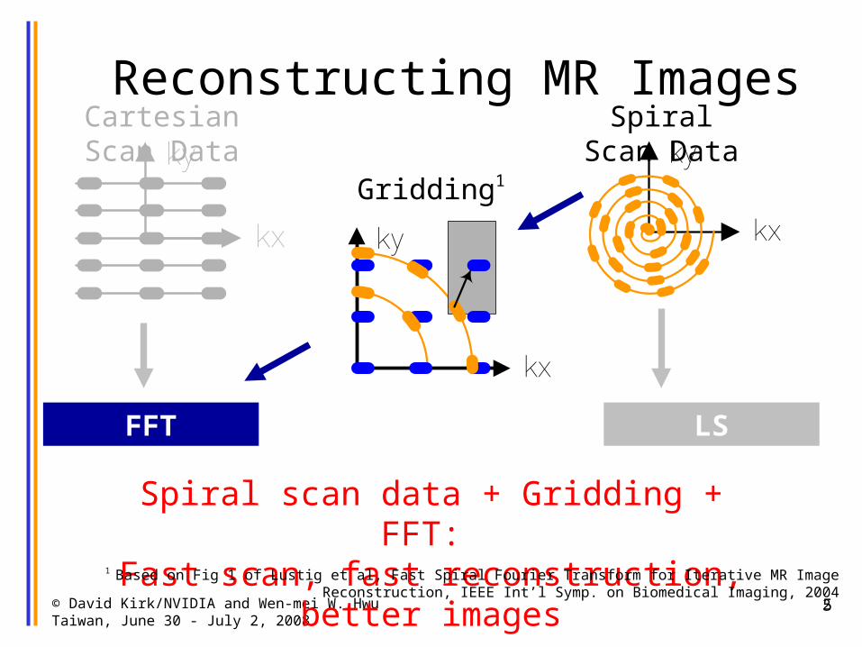
Reconstructing MR ImagesCartesian Scan Data Spiral Scan Data
Gridding1
FFT LS
Spiral scan data + Gridding + FFT: Fast scan, fast reconstruction, better images
2
kx
ky
kx
kykx
ky
1 Based on Fig 1 of Lustig et al, Fast Spiral Fourier Transform for Iterative MR Image Reconstruction, IEEE Int’l Symp. on Biomedical Imaging, 2004

© David Kirk/NVIDIA and Wen-mei W. HwuTaiwan, June 30 - July 2, 2008
6
Reconstructing MR ImagesCartesian Scan Data Spiral Scan Data
Gridding
FFT Least-Squares (LS)
Spiral scan data + LSSuperior images at expense of significantly more computation
2
kx
ky
kx
ky kx
ky

© David Kirk/NVIDIA and Wen-mei W. HwuTaiwan, June 30 - July 2, 2008
7
An Exciting Revolution - Sodium Map of the Brain
• Images of sodium in the brain– Requires powerful scanner (9.4 Tesla)– Very large number of samples for increased SNR– Requires high-quality reconstruction
• Enables study of brain-cell viability before anatomic changes occur in stroke and cancer treatment – within days!
Courtesy of Keith Thulborn and Ian Atkinson, Center for MR Research, University of Illinois at Chicago

© David Kirk/NVIDIA and Wen-mei W. HwuTaiwan, June 30 - July 2, 2008
8
Least-Squares ReconstructiondFFF HH
Compute Q = FHF
Acquire Data
Compute FHd
Find ρ
• Q depends only on scanner configuration
• FHd depends on scan data• ρ found using linear solver
• Accelerate Q and FHd on G80– Q: 1-2 days on CPU
– FHd: 6-7 hours on CPU
– ρ: 1.5 minutes on CPU
5

© David Kirk/NVIDIA and Wen-mei W. HwuTaiwan, June 30 - July 2, 2008
9
Algorithms to Accelerate
for (m = 0; m < M; m++) {
phi[m] = rPhi[m]*rPhi[m] + iPhi[m]*iPhi[m]
for (n = 0; n < N; n++) { exp = 2*PI*(kx[m]*x[n] + ky[m]*y[n] + kz[m]*z[n]) rQ[n] += phi[m]*cos(exp) iQ[n] += phi[m]*sin(exp) }
}
Compute Q • FHd is nearly identical• Scan data
– M = # scan points– kx, ky, kz = 3D scan data
• Pixel data– N = # pixels– x, y, z = input 3D pixel
data– Q = output pixel data
• Complexity is O(MN)• Inner loop
– 10 FP MUL or ADD ops– 2 FP trig ops– 10 loads
6

© David Kirk/NVIDIA and Wen-mei W. HwuTaiwan, June 30 - July 2, 2008
10
From C to CUDA: Step 1What unit of work is assigned to each thread?
7
for (m = 0; m < M; m++) { phi[m] = rPhi[m]*rPhi[m] + iPhi[m]*iPhi[m]
for (n = 0; n < N; n++) { exp = 2*PI*(kx[m]*x[n] + ky[m]*y[n] + kz[m]*z[n]) rQ[n] += phi[m]*cos(exp) iQ[n] += phi[m]*sin(exp) }}

© David Kirk/NVIDIA and Wen-mei W. HwuTaiwan, June 30 - July 2, 2008
118
for (m = 0; m < M; m++) { phi[m] = rPhi[m]*rPhi[m] + iPhi[m]*iPhi[m]
for (n = 0; n < N; n++) { exp = 2*PI*(kx[m]*x[n] + ky[m]*y[n] + kz[m]*z[n]) rQ[n] += phi[m]*cos(exp) iQ[n] += phi[m]*sin(exp) }}
How does loop interchange help?
for (n = 0; n < N; n++) { for (m = 0; m < M; m++) { phi[m] = rPhi[m]*rPhi[m] + iPhi[m]*iPhi[m] exp = 2*PI*(kx[m]*x[n] + ky[m]*y[n] + kz[m]*z[n]) rQ[n] += phi[m]*cos(exp) iQ[n] += phi[m]*sin(exp) }}
From C to CUDA: Step 1What unit of work is assigned to each thread?
© David Kirk/NVIDIA and Wen-mei W. HwuTaiwan, June 30 - July 2, 2008
129
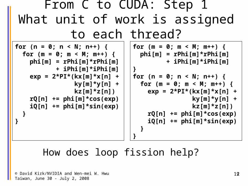
for (n = 0; n < N; n++) { for (m = 0; m < M; m++) { phi[m] = rPhi[m]*rPhi[m] + iPhi[m]*iPhi[m] exp = 2*PI*(kx[m]*x[n] + ky[m]*y[n] + kz[m]*z[n]) rQ[n] += phi[m]*cos(exp) iQ[n] += phi[m]*sin(exp) }}
How does loop fission help?
for (m = 0; m < M; m++) { phi[m] = rPhi[m]*rPhi[m] + iPhi[m]*iPhi[m]}for (n = 0; n < N; n++) { for (m = 0; m < M; m++) { exp = 2*PI*(kx[m]*x[n] + ky[m]*y[n] + kz[m]*z[n]) rQ[n] += phi[m]*cos(exp) iQ[n] += phi[m]*sin(exp) }}
From C to CUDA: Step 1What unit of work is assigned to each thread?

© David Kirk/NVIDIA and Wen-mei W. HwuTaiwan, June 30 - July 2, 2008
1310
for (m = 0; m < M; m++) { phi[m] = rPhi[m]*rPhi[m] + iPhi[m]*iPhi[m]}
for (n = 0; n < N; n++) { for (m = 0; m < M; m++) { exp = 2*PI*(kx[m]*x[n] + ky[m]*y[n] + kz[m]*z[n]) rQ[n] += phi[m]*cos(exp) iQ[n] += phi[m]*sin(exp) }}
From C to CUDA: Step 1What unit of work is assigned to each thread?
}• phi kernel• Each thread
computes phi at one scan point (each thread corresponds to one loop iteration)
}• Q kernel• Each thread
computes Q at one pixel (each thread corresponds to one outer loop iteration)

© David Kirk/NVIDIA and Wen-mei W. HwuTaiwan, June 30 - July 2, 2008
14
Tiling of Scan DataLS recon uses multiple grids
– Each grid operates on all pixels– Each grid operates on a distinct
subset of scan data– Each thread in the same grid
operates on a distinct pixel
for (m = 0; m < M/32; m++) { exp = 2*PI*(kx[m]*x[n] + ky[m]*y[n] + kz[m]*z[n]) rQ[n] += phi[m]*cos(exp) iQ[n] += phi[m]*sin(exp)}
12
Thread n operates on pixel n:
Grid MTB0 TB1 TBN………………..
………………SM 0 SM 15
Instruction Unit
32KB Register File 8KB Constant Cache
SP0 SP7
SFU0 SFU1
SM Array
………………….
Off-Chip Memory (Global, Constant)
xyz
rQiQ
kxkykzphi
Grid 1TB0 TB1 TBN………………..Grid 0TB0 TB1 TBN………………..
Pixel Data Scan Data

© David Kirk/NVIDIA and Wen-mei W. HwuTaiwan, June 30 - July 2, 2008
15
• LS recon uses multiple grids– Each grid operates on all pixels– Each grid operates on a distinct
subset of scan data– Each thread in the same grid
operates on a distinct pixel
Tiling of Scan Data
12
for (m = 31M/32; m < 32M/32; m++) { exp = 2*PI*(kx[m]*x[n] + ky[m]*y[n] + kz[m]*z[n]) rQ[n] += phi[m]*cos(exp) iQ[n] += phi[m]*sin(exp)}
Thread n operates on pixel n:
Grid MTB0 TB1 TBN………………..
………………SM 0 SM 15
Instruction Unit
32KB Register File 8KB Constant Cache
SP0 SP7
SFU0 SFU1
SM Array
………………….
Off-Chip Memory (Global, Constant)
xyz
rQiQ
kxkykzphi
Grid 1TB0 TB1 TBN………………..Grid 0TB0 TB1 TBN………………..
Pixel Data Scan Data

© David Kirk/NVIDIA and Wen-mei W. HwuTaiwan, June 30 - July 2, 2008
1613
Q(float* x,y,z,rQ,iQ,kx,ky,kz,phi, int startM,endM){ n = blockIdx.x*TPB + threadIdx.x for (m = startM; m < endM; m++) { exp = 2*PI*(kx[m]*x[n] + ky[m]*y[n] + kz[m]*z[n]) rQ[n] += phi[m] * cos(exp) iQ[n] += phi[m] * sin(exp) }}
From C to CUDA: Step 2Where are the potential bottlenecks?
Bottlenecks• Memory BW• Trig ops• Overheads
(branches, addr calcs)
© David Kirk/NVIDIA and Wen-mei W. HwuTaiwan, June 30 - July 2, 2008
17
Step 3: Overcoming bottlenecks
14
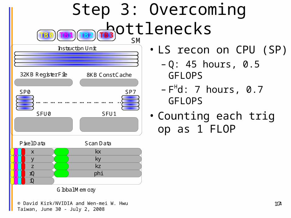
• LS recon on CPU (SP) – Q: 45 hours, 0.5 GFLOPS
– FHd: 7 hours, 0.7 GFLOPS
• Counting each trig op as 1 FLOP
TB0 TB1 TB2
Global Memory
xyz
rQiQ
kxkykzphi
SMTB3
32KB Register File 8KB Const Cache
……………………………..
Instruction Unit
SFU0 SFU1
SP0 SP7
Pixel Data Scan Data

© David Kirk/NVIDIA and Wen-mei W. HwuTaiwan, June 30 - July 2, 2008
18
Step 3: Overcoming Bottlenecks (Mem BW)
15
TB0 TB1 TB2
Global Memory
xyz
rQiQ
kxkykzphi
SMTB3
32KB Register File 8KB Const Cache
……………………………..
Instruction Unit
SFU0 SFU1
SP0 SP7
exp = 2*PI*(kx[m] * x[n] + ky[m] * y[n] + kz[m] * z[n])rQ[n] += phi[m] * cos(exp)iQ[n] += phi[m] * sin(exp)
Pixel Data Scan Data
• Register allocate pixel data– Inputs (x, y, z); Outputs (rQ, iQ)
• Exploit temporal and spatial locality in access to scan data– Constant memory + constant caches
– Shared memory

© David Kirk/NVIDIA and Wen-mei W. HwuTaiwan, June 30 - July 2, 2008
19
Step 3: Overcoming Bottlenecks (Mem BW)
• Register allocation of pixel data– Inputs (x, y, z); Outputs (rQ, iQ)
– FP arithmetic to off-chip loads: 2 to 1
• Performance– 5.1 GFLOPS (Q), 5.4 GFLOPS (FHd)
• Still bottlenecked on memory BW
16
TB0 TB1 TB2
Global Memory
xyz
rQiQ
kxkykzphi
SMTB3
32KB Register File 8KB Const Cache
……………………………..
Instruction Unit
SFU0 SFU1
SP0 SP7
exp = 2*PI*(kx[m] * x[n] + ky[m] * y[n] + kz[m] * z[n])rQ[n] += phi[m] * cos(exp)iQ[n] += phi[m] * sin(exp)
Pixel Data Scan Data

© David Kirk/NVIDIA and Wen-mei W. HwuTaiwan, June 30 - July 2, 2008
20
Step 3: Overcoming Bottlenecks (Mem BW)
• Old bottleneck: off-chip BW– Solution: constant memory
– FP arithmetic to off-chip loads: 284 to 1
• Performance– 18.6 GFLOPS (Q), 22.8 GFLOPS
(FHd)
• New bottleneck: trig operations17
TB0 TB1 TB2
Global Memory
xyz
rQiQ
kxkykzphi
SMTB3
32KB Register File 8KB Const Cache
……………………………..
Instruction Unit
SFU0 SFU1
SP0 SP7
exp = 2*PI*(kx[m] * x[n] + ky[m] * y[n] + kz[m] * z[n])rQ[n] += phi[m] * cos(exp)iQ[n] += phi[m] * sin(exp)
Constant Memory
Pixel Data Scan Data

© David Kirk/NVIDIA and Wen-mei W. HwuTaiwan, June 30 - July 2, 2008
21
Sidebar: Estimating Off-Chip Loads with Const Cache
• How can we approximate the number of off-chip loads when using the constant caches?
• Given: 128 tpb, 4 blocks per SM, 256 scan points per grid
• Assume no evictions due to cache conflicts
• 7 accesses to global memory per thread (x, y, z, rQ x 2, iQ x 2)– 4 blocks/SM * 128 threads/block * 7 accesses/thread = 3,584 global mem accesses
• 4 accesses to constant memory per scan point (kx, ky, kz, phi)– 256 scan points * 4 loads/point = 1,024 constant mem accesses
• Total off-chip memory accesses = 3,584 + 1,024 = 4,608
• Total FP arithmetic ops = 4 blocks/SM * 128 threads/block * 256 iters/thread * 10 ops/iter = 1,310,720
• FP arithmetic to off-chip loads: 284 to 1
18
© David Kirk/NVIDIA and Wen-mei W. HwuTaiwan, June 30 - July 2, 2008
22
Step 3: Overcoming Bottlenecks (Trig)
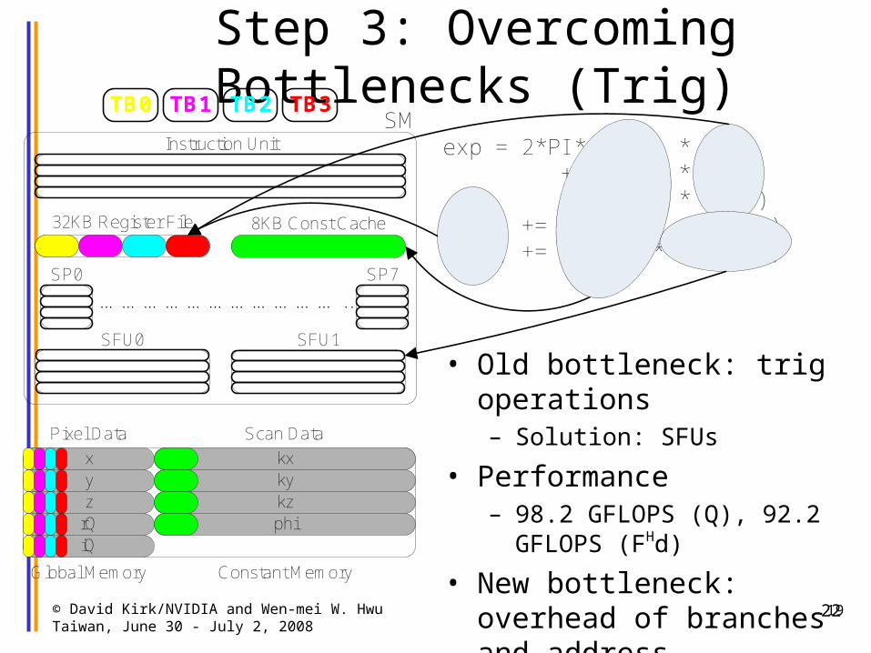
• Old bottleneck: trig operations– Solution: SFUs
• Performance– 98.2 GFLOPS (Q), 92.2 GFLOPS
(FHd)
• New bottleneck: overhead of branches and address calculations 19
TB0 TB1 TB2
xyz
rQiQ
kxkykzphi
SMTB3
32KB Register File 8KB Const Cache
……………………………..
Instruction Unit
SFU0 SFU1
SP0 SP7
exp = 2*PI*(kx[m] * x[n] + ky[m] * y[n] + kz[m] * z[n])rQ[n] += phi[m] * cos(exp)iQ[n] += phi[m] * sin(exp)
Global Memory Constant Memory
Pixel Data Scan Data
© David Kirk/NVIDIA and Wen-mei W. HwuTaiwan, June 30 - July 2, 2008
23
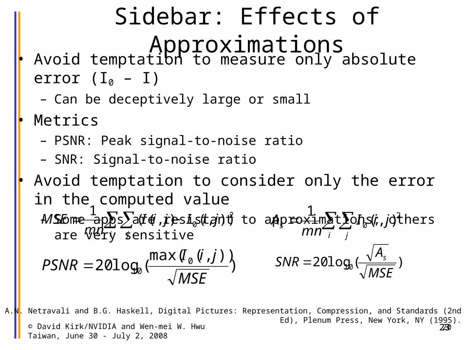
Sidebar: Effects of Approximations• Avoid temptation to measure only absolute error (I0 – I)
– Can be deceptively large or small
• Metrics– PSNR: Peak signal-to-noise ratio
– SNR: Signal-to-noise ratio
• Avoid temptation to consider only the error in the computed value– Some apps are resistant to approximations; others are very sensitive
20
i j
jiIjiImn
MSE 20 )),(),((
1
))),(max(
(log20 010
MSE
jiIPSNR
i j
s jiImn
A 20 ),(
1
)(log20 10MSE
ASNR s
A.N. Netravali and B.G. Haskell, Digital Pictures: Representation, Compression, and Standards (2nd Ed), Plenum Press, New York, NY (1995).
© David Kirk/NVIDIA and Wen-mei W. HwuTaiwan, June 30 - July 2, 2008
24
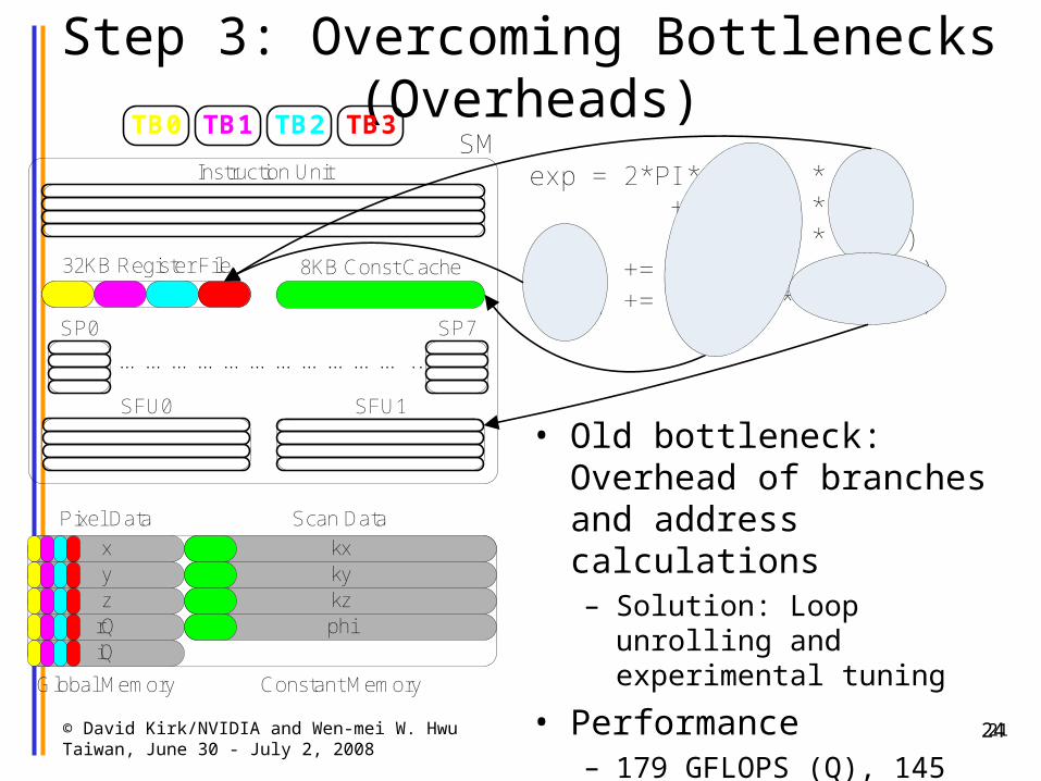
Step 3: Overcoming Bottlenecks (Overheads)
• Old bottleneck: Overhead of branches and address calculations– Solution: Loop unrolling and
experimental tuning
• Performance– 179 GFLOPS (Q), 145 GFLOPS
(FHd) 21
TB0 TB1 TB2
xyz
rQiQ
kxkykzphi
SMTB3
32KB Register File 8KB Const Cache
……………………………..
Instruction Unit
SFU0 SFU1
SP0 SP7
exp = 2*PI*(kx[m] * x[n] + ky[m] * y[n] + kz[m] * z[n])rQ[n] += phi[m] * cos(exp)iQ[n] += phi[m] * sin(exp)
Global Memory Constant Memory
Pixel Data Scan Data

© David Kirk/NVIDIA and Wen-mei W. HwuTaiwan, June 30 - July 2, 2008
25
Experimental Tuning: Tradeoffs• In the Q kernel, three parameters are natural candidates for
experimental tuning– Loop unrolling factor (1, 2, 4, 8, 16)
– Number of threads per block (32, 64, 128, 256, 512)
– Number of scan points per grid (32, 64, 128, 256, 512, 1024, 2048)
• Can’t optimize these parameters independently– Resource sharing among threads (register file, shared memory)
– Optimizations that increase a thread’s performance often increase the thread’s resource consumption, reducing the total number of threads that execute in parallel
• Optimization space is not linear– Threads are assigned to SMs in large thread blocks
– Causes discontinuity and non-linearity in the optimization space
22

© David Kirk/NVIDIA and Wen-mei W. HwuTaiwan, June 30 - July 2, 2008
26
Experimental Tuning: Example
Increase in per-thread performance, but fewer threads:Lower overall performance
TB0 TB1 TB2
32KB Register File
………
16KB Shared Memory
SFU0 SFU1
SP0 SP7
(a) Pre-“optimization”
Core Computation
Thread Contexts
SP Utilization
Area determines overall performance
32KB Register File
16KB Shared Memory
SFU0 SFU1
………
SP0 SP7
(b) Post-“optimization”
Insufficient registers to allocate 3 blocks
Thread Contexts
X
23

© David Kirk/NVIDIA and Wen-mei W. HwuTaiwan, June 30 - July 2, 2008
27
0
5
10
15
20
25
30
35
40
32 64 128 256 512 1024 2048
Scan points per grid
Tim
e (s
)Experimental Tuning: Scan Points Per Grid
24

© David Kirk/NVIDIA and Wen-mei W. HwuTaiwan, June 30 - July 2, 2008
28
Sidebar: Cache-Conscious Data Layout
• kx, ky, kz, and phi components of same scan point have spatial and temporal locality– Prefetching
– Caching
• Old layout does not fully leverage that locality
• New layout does fully leverage that locality
25
kx[i] ky[i] kz[i] phi[i]
Constant Memory
Scan Data
kxkykzphi
kx[i]ky[i]ky[i]phi[i]
Constant Memory
Scan Data

© David Kirk/NVIDIA and Wen-mei W. HwuTaiwan, June 30 - July 2, 2008
29
Experimental Tuning: Scan Points Per Grid (Improved Data Layout)
0
2
4
6
8
10
12
14
16
32 64 128 256 512 1024 2048
Scan points per grid
Tim
e (s
)
26

© David Kirk/NVIDIA and Wen-mei W. HwuTaiwan, June 30 - July 2, 2008
30
Experimental Tuning: Loop Unrolling Factor
27
2
4
6
8
10
12
14
1 2 4 8 16
Loop unrolling factor
Tim
e (s
)

© David Kirk/NVIDIA and Wen-mei W. HwuTaiwan, June 30 - July 2, 2008
31
Sidebar: Optimizing the CPU Implementation
• Optimizing the CPU implementation of your application is very important– Often, the transformations that increase performance on CPU also
increase performance on GPU (and vice-versa)
– The research community won’t take your results seriously if your baseline is crippled
• Useful optimizations– Data tiling
– SIMD vectorization (SSE)
– Fast math libraries (AMD, Intel)
– Classical optimizations (loop unrolling, etc)
• Intel compiler (icc, icpc)
28

© David Kirk/NVIDIA and Wen-mei W. HwuTaiwan, June 30 - July 2, 2008
32
Summary of ResultsQ FHd
Reconstruction Run Time (m)
GFLOP Run Time (m)
GFLOP Linear Solver (m)
Recon. Time (m)
Gridding + FFT
(CPU, DP)
N/A N/A N/A N/A N/A 0.39
LS (CPU, DP) 4009.0 0.3 518.0 0.4 1.59 519.59
LS (CPU, SP) 2678.7 0.5 342.3 0.7 1.61 343.91
LS (GPU, Naïve) 260.2 5.1 41.0 5.4 1.65 42.65
LS (GPU, CMem)
72.0 18.6 9.8 22.8 1.57 11.37
LS (GPU, CMem,
SFU)
13.6 98.2 2.4 92.2 1.60 4.00
LS (GPU, CMem,
SFU, Exp)
7.5 178.9 1.5 144.5 1.69 3.19
29
8X

© David Kirk/NVIDIA and Wen-mei W. HwuTaiwan, June 30 - July 2, 2008
33
Summary of Results
30
Q FHdReconstruction Run Time (m) GFLOP Run Time
(m)GFLOP Linear
Solver (m)Recon. Time
(m)
Gridding + FFT
(CPU, DP)
N/A N/A N/A N/A N/A 0.39
LS (CPU, DP) 4009.0 0.3 518.0 0.4 1.59 519.59
LS (CPU, SP) 2678.7 0.5 342.3 0.7 1.61 343.91
LS (GPU, Naïve) 260.2 5.1 41.0 5.4 1.65 42.65
LS (GPU, CMem) 72.0 18.6 9.8 22.8 1.57 11.37
LS (GPU, CMem,
SFU)
13.6 98.2 2.4 92.2 1.60 4.00
LS (GPU, CMem,
SFU, Exp)
7.5 178.9 1.5 144.5 1.69 3.19
108X228X357X

© David Kirk/NVIDIA and Wen-mei W. HwuTaiwan, June 30 - July 2, 2008
34
Questions?
31
+
=
Scanner image released distributed under GNU Free Documentation License.GeForce 8800 GTX image obtained from http://www.nvnews.net/previews/geforce_8800_gtx/index.shtml

© David Kirk/NVIDIA and Wen-mei W. HwuTaiwan, June 30 - July 2, 2008
35
Algorithms to Accelerate
for (K = 0; K < numK; K++) rRho[K] = rPhi[K]*rD[K] + iPhi[K]*iD[K] iRho[K] = rPhi[K]*iD[K] - iPhi[K]*rD[K]
for (X = 0; X < numP; X++) for (K = 0; K < numK; K++) exp = 2*PI*(kx[K]*x[X] + ky[K]*y[X] + kz[K]*z[X]) cArg = cos(exp) sArg = sin(exp) rFH[X] += rRho[K]*cArg – iRho[K]*sArg iFH[X] += iRho[K]*cArg + rRho[K]*sArg
Compute FHd
• Inner loop– 14 FP MUL or ADD
ops
– 4 FP trig ops
– 12 loads (naively)

© David Kirk/NVIDIA and Wen-mei W. HwuTaiwan, June 30 - July 2, 2008
36
Experimental Methodology
• Reconstruct a 3D image of a human brain1
– 3.2 M scan data points acquired via 3D spiral scan– 256K pixels
• Compare performance several reconstructions– Gridding + FFT recon1 on CPU (Intel Core 2 Extreme Quadro)– LS recon on CPU (double-precision, single-precision)– LS recon on GPU (NVIDIA GeForce 8800 GTX)
• Metrics– Reconstruction time: compute FHd and run linear solver
– Run time: compute Q or FHd
1 Courtesy of Keith Thulborn and Ian Atkinson, Center for MR Research, University of Illinois at Chicago8