α-ψ-ϕ-contractive mappings in ordered partial b-metricspaces

Aiman A. MukheimerDepartment of Mathematical Sciences, Prince Sultan University

Riyadh, Saudi Arabia 11586E-mail: mukheimer@psu.edu.sa

Abstract

In this paper, we introduce the concept of α-ψ-ϕ-contractive self mapping in com-plete ordered partial b−metric space, and we study the existence of fixed points forsuch mappings under some conditions. Presented theorems in this paper extend andgeneralize the results derived by Mustafa et al. in [17]. Some examples are given toillustrate the main results.

1 Introduction

Fixed point theory is one of the most popular tool in nonlinear analysis. Most of the gen-eralizations for metric fixed point theorems usually start from Banach contraction principle[9]. It is not easy to point out all the generalizations of this principle. In 1989, Bakhtin[8] introduced the concept of a b-metric space as a generalization of metric spaces. In 1993,Czerwik [10, 11] extended many results related to the b−metric spaces. In 1994, Matthews[15] introduced the concept of partial metric space in which the self distance of any point ofspace may not be zero. In 1996, O’Neill generalized the concept of partial metric space byadmitting negative distances. In 2013, Shukla [19] generalized both the concept of b-metricand partial metric spaces by introducing the partial b-metric spaces. For example, many au-thors recently studied this principle and its generalizations in different types of metric spaces[4, 5, 1, 2]. Close to our interest in this paper some authors studied some fixed point theoremsin the so called b−metric space [16, 20, 21]. After then, some authors started to prove α-ψversions of of certain fixed point theorems in different type metric spaces [3, 12, 6]. Mustafain [17], gave a generalization of Banach’s contraction principles in a complete ordered partialb−metric space by introducing a generalized (α, ψ)s−weakly contractive mapping.

In this paper, we generalize a result of Mustafa in [17], by introducing the α-ψ-ϕ-contractive mapping in a complete ordered partial b-metric space.

Definition 1.1. [7] Let X be a nonempty set and let s ≥ 1 be a given real number. A functiond : X × X → [0,∞) is called a b-metric if for all x, y, z ∈ X the following conditions aresatisfied:

1

(i) d(x, y) = 0 if and only if x = y;(ii) d(x, y) = d(y, x);(iii) d(x, y) ≤ s[d(x, z) + d(z, y)].The pair (X, d) is called a b-metric space. The number s ≥ 1 is called the coefficient of(X, d).

Definition 1.2. [15] Let X be a nonempty set. A function p : X ×X → [0,∞) is called apartial metric if for all x, y, z ∈ X the following conditions are satisfied:(i) x = y if and only if p(x, x) = p(x, y) = p(y, y);(ii) p(x, x) ≤ p(x, y);(iii) p(x, y) = p(y, x);(iv) p(x, y) ≤ p(x, z) + p(z, y)− p(z, z).The pair (X, d) is called a partial metric space.

Remark 1.1. It is clear that the partial metric space need not be a b−metric spaces , sincein a partial metric space if p(x, y) = 0 implies p(x, x) = p(x, y) = p(y, y) = 0 then x = y.But in a partial metric space if x = y then p(x, x) = p(x, y) = p(y, y) may not be equal zero.Therefore the partial metric space may not be a b−metric space.

On the other hand, Shukla[19] introduced the notion of a partial b−metric space asfollows:

Definition 1.3. [19] Let X be a nonempty set and s ≥ 1 be a given real number. A functionpb : X×X → [0,∞) is called a partial b−metric if for all x, y, z ∈ X the following conditionsare satisfied:(i) x = y if and only if pb(x, x) = pb(x, y) = pb(y, y);(ii) pb(x, x) ≤ pb(x, y);(iii) pb(x, y) = pb(y, x);(iv) pb(x, y) ≤ s[pb(x, z) + pb(z, y)]− pb(z, z).The pair (X, pb) is called a partial b−metric space. The number s ≥ 1 is called the coefficientof (X, pb).

Remark 1.2. The class of partial b−metric space (X, pb) is effectively larger than the classof partial metric space, since a partial metric space is a special case of a partial b−metricspace (X, pb) when s = 1. Also, the class of partial b−metric space (X, pb) is effectivelylarger than the class of b−metric space, since a b−metric space is a special case of a partialb−metric space (X, pb) when the self distance p(x, x) = 0.

The following examples shows that a partial b−metric on X need not be a partial metric,nor a b−mertic on X see also [17], [19].

Example 1.1. [19] Let X = [0,∞). Define a function pb : X × X → [0,∞) such thatpb(x, y) = [max{x, y}]2 + |x− y|2 For all x, y ∈ X. Then (X, pb) is a partial b-metric spaceon X with the coefficient s = 2 > 1. But, pb is not a b-metric nor a partial metric on X.

Proposition 1.1. [19] Let X be a nonempty set, and let p be a partial metric and d be ab-metric with the coefficient s ≥ 1 on X. Then the function pb : X ×X → [0,∞) defined bypb(x, y) = p(x, y) + d(x, y) For all x, y ∈ X, is a partial b-metric on X with the coefficient s.

2

Proposition 1.2. [19] Let (X, p) be a partial metric space and q ≥ 1. Then (X, pb) is apartial b-metric space with coefficient s = 2q−1, where pb is defined by pb(x, y) = [p(x, y)]q.

Definition 1.4. [14] A function ψ : [0,∞) → [0,∞) is called an altering distance functionif the following properties are satisfied:1. ψ is continuous and nondecreasing;2. ψ(t) = 0 if and only if t = 0.

On the other hand, Mustafa[17] modify the Definition 1.3 in order that each partialb-metric pb generates a b-metric dpb as follows:

Definition 1.5. [17] Let X be a nonempty set and s ≥ 1 be a given real number. A functionpb : X ×X → [0,∞) is a partial b-metric if for all x, y, z ∈ X the following conditions aresatisfied:(i) x = y if and only if pb(x, x) = pb(x, y) = pb(y, y);(ii) pb(x, x) ≤ pb(x, y);(iii) pb(x, y) = pb(y, x);(iv) pb(x, y) ≤ s[pb(x, z) + pb(z, y)− pb(z, z)] + (1−s

2)(pb(x, x) + pb(y, y)).

The pair (X, pb) is called a partial b-metric space. The number s ≥ 1 is called the coefficientof (X, pb).

Example 1.2 (see also[17]). Let X = R is the set of real numbers. Consider the metricspace (X, d) where d is the Euclidean distance metric d(x, y) = |x − y| for all x, y ∈ X.Define pb(x, y) = (x − y)2 + 5 for all x, y ∈ X. Then pb is a partial b-metric on X withs = 2, but it is not a partial metric on X. To see this, Let x = 1,y = 4 and z = 2. Then

pb(1, 4) = (1− 4)2 + 5 = 14 � pb(1, 2) + pb(2, 4)− pb(2, 2) = 6 + 9− 5 = 10.

Also, pb is not a b-metric since pb(x, x) 6= 0 for all x ∈ X.

Proposition 1.3. [17] Every partial b-metric pb defines a b-metric dpb, where

dpb(x, y) = 2pb(x, y)− pb(x, x)− pb(y, y), for all x, y ∈ X (1.1)

Definition 1.6. [17] A sequence {xn} in a partial b-metric space (X, pb) is said to be:(i) pb-convergent to a point x ∈ X if limn→∞ pb(x, xn) = pb(x, x);(ii) a pb−Cauchy sequence if limn,m→∞ pb(xn, xm)exists (and is finite);(iii) A partial b−metric space (X, pb) is said to be pb-complete if every pb-Cauchy sequence{xn} in X pb converges to a point x ∈ X such that

limn,m→∞

pb(xn, xm) = limn→∞

pb(xn, x) = pb(x, x). (1.2)

Lemma 1.1. [17] A sequence {xn} is a pb-Cauchy sequence in a partial b−metric space(X, pb) if and only if it is a b-Cauchy sequence in the b-metric space (X, dpb).

Lemma 1.2. [17] A partial b-metric space (X, pb) is pb-complete if and only if the b-metricspace (X, dpb) is b-complete. Moreover, limn→∞ dpb(xn, xm) = 0 if and only if

limn→∞

pb(x, xn) = limn,m→∞

pb(x, xm) = pb(x, x). (1.3)

3

Lemma 1.3. [17] Let (X, pb) be a partial b-metric space with the coefficient s > 1 andsuppose that {xn} and{yn} are convergent to x and y, respectively. Then we have

1

s2pb(x, y)− 1

spb(x, x)− pb(y, y) ≤ lim inf

n→∞pb(xn, yn)

≤ lim supn→∞

pb(xn, yn)

≤ spb(x, x) + s2pb(y, y) + s2pb(x, y).

Definition 1.7. [13] Let (X,�) be a partially ordered set and T : X → X be a mapping.We say that T is nondecreasing with respect to � if

x, y ∈ X, x � y ⇒ Tx � Ty.

Definition 1.8. [13] Let (X,�) be a partially ordered set. A sequence {xn} is said to benondecreasing with respect to � if xn � xn+1 for all n ∈ N.

Definition 1.9. [17] A triple (X,�, pb) is called an ordered partial b-metric space if (X,�)is a partially ordered set and pb is a partial b-metric on X.

Definition 1.10. Let (X, pb) be a partial b-metric space and T : X −→ X be a givenmapping. We say that T is α-admissible if x, y ∈ X, α(x, y) ≥ 1 implies that α(Tx, Ty) ≥ 1.Also we say that T is Lα-admissible (Rα-admissible) if x, y ∈ X, α(x, y) ≥ 1 implies thatα(Tx, y) ≥ 1(α(x, Ty) ≥ 1).

Example 1.3. [18] Let X = (0,∞). Define T : X → X and α : X × X → [0,∞) byTx = lnx for all x ∈ X and

α(x, y) =

{2 if x ≥ y,0 if x < y.

Then, T is α-admissible.

Example 1.4. [18] Let X = [0,∞). Define T : X → X and α : X × X → [0,∞) byTx =

√x for all x ∈ X and

α(x, y) =

{ex−y if x ≥ y,0 if x < y.

Then, T is α-admissible.

2 Main result

We now introduce the α-ψ-ϕ-contractive self mapping on partial b-metric space.

Definition 2.1. Let (X, pb) be a partial b-metric space with the coefficient s ≥ 1. We saythat a mapping T : X → X is an α-ψ-ϕ-contractive mapping if there exist two alteringdistance functions ψ, ϕ and α : X ×X :→ [0,∞) such that

α(x, y)ψ(spb(Tx, Ty)) ≤ ψ(MTs (x, y))− ϕ(MT

s (x, y)) (2.1)

for all comparable x, y ∈ X.

4

where

MTs (x, y) = max{pb(x, y), pb(x, Tx), pb(y, Ty),

pb(x, Ty) + pb(y, Tx)

2s}. (2.2)

Theorem 2.1. Let (X,�, pb) be a pb-complete ordered partial b-metric space with the co-efficient s ≥ 1. Let T : X → X be an an α-ψ-ϕ-contractive mapping. Suppose that thefollowing conditions hold:

(1) T is α-admissible and Lα-admissible (or Rα-admissible );(2) there exists x1 ∈ X such that x1 � Tx1 and α(x1, Tx1) ≥ 1;(3) T is continuous, nondecreasing, with respect to � and if T nx1 → z then α(z, z) ≥ 1 .Then, T has a fixed point.

Proof. Let x1 ∈ X such that x1 � Tx1 and α(x1, Tx1) ≥ 1. Define a sequence {xn} in Xby xn+1 = Txn for all n ≥ 1. We have x2 = Tx1 � Tx2 = x3 since x1 � Tx1 and T isnondecreasing. Also, x3 = Tx2 � Tx3 = x4 since x2 � Tx2 and T is nondecreasing. Byinduction, we get

x1 � x2 � x3 � · · · � xn � xn+1 � · · ·.

If xn = xn+1 for some n ∈ N, then x = xn is a fixed point of T and the proof is finished. Sowe may assume that xn 6= xn+1 for all n ∈ N. Since T is α-admissible, we deduce

α(x1, Tx1) = α(x1, x2) ≥ 1⇒ α(Tx1, Tx2) = α(x2, x3) ≥ 1.

By induction on n we getα(xn, xn+1) ≥ 1 (2.3)

for all n ∈ N.Hence, by applying the α-ψ-ϕ-contractive condition and using (2.3) for all n ∈ N we get

ψ(spb(xn+1, xn+2)) ≤ α(xn, xn+1)ψ(spb(Txn, Txn+1))

≤ ψ(MTs (xn, xn+1))− ϕ(MT

s (xn, xn+1)) (2.4)

where

MTs (xn, xn+1) = max{pb(xn, xn+1), pb(xn, Txn), pb(xn+1, Txx+1),

pb(xn, Txn+1) + pb(xn+1, Txn)

2s}

= max{pb(xn, xn+1), pb(xn+1, xx+2),

pb(xn, xn+2) + pb(xn+1, xn+1)

2s}

≤ max{pb(xn, xn+1), pb(xn+1, xx+2),

spb(xn, xn+1) + spb(xn+1, xn+2) + (1− s)pb(xn+1, xn+1)

2s}

= max{pb(xn, xn+1), pb(xn+1, xx+2)} (2.5)

5

From (2.4)and (2.5) we get

ψ(pb(xn+1, xn+2)) ≤ ψ(max{pb(xn, xn+1), pb(xn+1, xx+2)})−ϕ(max{pb(xn, xn+1), pb(xn+1, xx+2)}) (2.6)

Assume thatmax{pb(xn, xn+1), pb(xn+1, xx+2)} = pb(xn+1, xx+2)

then by using properties of ϕ, we deduce

ψ(pb(xn+1, xn+2)) ≤ ψ(pb(xn+1, xn+2))− ϕ(pb(xn+1, xn+2))

< ψ(pb(xn+1, xn+2)),

which is a contradiction. Thus,

ψ(pb(xn+1, xn+2)) ≤ ψ(pb(xn, xn+1))− ϕ(pb(xn, xn+1)). (2.7)

So the sequence {pb(xn+1, xn+2)} is nonnegative and nondecreasing for all n ∈ N. Hencethere exists r ≥ 0 such that

limn→∞

pb(xn+1, xn+2) = r.

Letting n→∞ in (2.7) , we have

ψ(r) ≤ ψ(r)− ϕ(r) ≤ ψ(r).

Therefore, ϕ(r) = 0, and hence r = 0. Thus,

limn→∞

pb(xn+1, xn+2) = 0. (2.8)

Now, we show that {xn} is a Cauchy sequence in (X, pb) which is equivalent to show that{xn} is a b-Cauchy sequence in (X, dpb). Assume not, that is, {xn} is not a b-Cauchy sequencein (X, dpb). Then there exist ε > 0 such that, for k > 0, there exist n(k) > m(k) > k forwhich we can which we can find two subsequences {xn(k)} and {xm(k)} of {xn} such thatn(k) is the smallest index for which

dpb(xm(k), xn(k)) ≥ ε, (2.9)

and

dpb(xm(k), xn(k)−1) < ε. (2.10)

Then we have

ε ≤ dpb(xm(k), xn(k)) ≤ sdpb(xm(k), xn(k)−1) + sdpb(xn(k)−1, xn(k))

< sε+ sdpb(xn(k)−1, xn(k)). (2.11)

Taking the upper limit for (2.10) as k →∞, we have

ε

s≤ lim inf

k→∞dpb(xm(k), xn(k)−1) ≤ lim sup

k→∞dpb(xm(k), xn(k)−1) ≤ ε. (2.12)

6

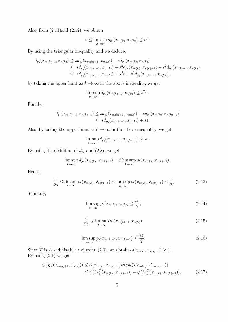
Also, from (2.11)and (2.12), we obtain

ε ≤ lim supk→∞

dpb(xm(k), xn(k)) ≤ sε.

By using the triangular inequality and we deduce,

dpb(xm(k)+1, xn(k)) ≤ sdpb(xm(k)+1, xm(k)) + sdpb(xm(k), xn(k))

≤ sdpb(xm(k)+1, xm(k)) + s2dpb(xm(k), xn(k)−1) + s2dpb(xn(k)−1, xn(k))

≤ sdpb(xm(k)+1, xm(k)) + s2ε+ s2dpb(xn(k)−1, xn(k)),

by taking the upper limit as k →∞ in the above inequality, we get

lim supk→∞

dpb(xm(k)+1, xn(k)) ≤ s2ε.

Finally,

dpb(xm(k)+1, xn(k)−1) ≤ sdpb(xm(k)+1, xm(k)) + sdpb(xm(k), xn(k)−1)

≤ sdpb(xm(k)+1, xm(k)) + sε.

Also, by taking the upper limit as k →∞ in the above inequality, we get

lim supk→∞

dpb(xm(k)+1, xn(k)−1) ≤ sε.

By using the definition of dpb and (2.8), we get

lim supk→∞

dpb(xm(k), xn(k)−1) = 2 lim supk→∞

pb(xm(k), xn(k)−1).

Hence,

ε

2s≤ lim inf

k→∞pb(xm(k), xn(k)−1) ≤ lim sup

k→∞pb(xm(k), xn(k)−1) ≤

ε

2, (2.13)

Similarly,

lim supk→∞

pb(xm(k), xn(k)) ≤sε

2, (2.14)

ε

2s≤ lim sup

k→∞pb(xm(k)+1, xn(k)), (2.15)

lim supk→∞

pb(xm(k)+1, xn(k)−1) ≤sε

2. (2.16)

Since T is Lα-admissible and using (2.3), we obtain α(xm(k), xn(k)−1) ≥ 1.By using (2.1) we get

ψ(spb(xm(k)+1, xn(k))) ≤ α(xm(k), xn(k)−1)ψ(spb(Txm(k), Txn(k)−1))

≤ ψ(MTs (xm(k), xn(k)−1))− ϕ(MT

s (xm(k), xn(k)−1)), (2.17)

7

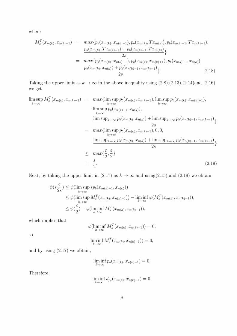
where

MTs (xm(k), xn(k)−1) = max{pb(xm(k), xn(k)−1), pb(xm(k), Txm(k)), pb(xn(k)−1, Txn(k)−1),

pb(xm(k), Txn(k)−1) + pb(xn(k)−1, Txm(k))

2s}

= max{pb(xm(k), xn(k)−1), pb(xm(k), xm(k)+1), pb(xn(k)−1, xn(k)),

pb(xm(k), xn(k)) + pb(xn(k)−1, xm(k)+1)

2s} (2.18)

Taking the upper limit as k →∞ in the above inequality using (2.8),(2.13),(2.14)and (2.16)we get

lim supk→∞

MTs (xm(k), xn(k)−1) = max{lim sup

k→∞pb(xm(k), xn(k)−1), lim sup

k→∞pb(xm(k), xm(k)+1),

lim supk→∞

pb(xn(k)−1, xn(k)),

lim supk→∞ pb(xm(k), xn(k)) + lim supk→∞ pb(xn(k)−1, xm(k)+1)

2s}

= max{lim supk→∞

pb(xm(k), xn(k)−1), 0, 0,

lim supk→∞ pb(xm(k), xn(k)) + lim supk→∞ pb(xn(k)−1, xm(k)+1)

2s}

≤ max{ε2,ε

2}

=ε

2. (2.19)

Next, by taking the upper limit in (2.17) as k →∞ and using(2.15) and (2.19) we obtain

ψ(sε

2s) ≤ ψ(lim sup

k→∞spb(xm(k)+1, xn(k)))

≤ ψ(lim supk→∞

MTs (xm(k), xn(k)−1))− lim inf

k→∞ϕ(MT

s (xm(k), xn(k)−1)),

≤ ψ(ε

2)− ϕ(lim inf

k→∞MT

s (xm(k), xn(k)−1)),

which implies thatϕ(lim inf

k→∞MT

s (xm(k), xn(k)−1)) = 0,

solim infk→∞

MTs (xm(k), xn(k)−1)) = 0,

and by using (2.17) we obtain,

lim infk→∞

pb(xm(k), xn(k)−1) = 0.

Therefore,lim infk→∞

dpb(xm(k), xn(k)−1) = 0,

8

which is a contradiction with (2.13). Thus, the sequence is a b-Cauchy in the b-metric space(X, dpb). Since (X, pb) is pb-complete, then (X, dpb) is a b-complete b-metric space. So, itfollows from the completeness that there exist z ∈ X such that,

limn→∞

dpb(xn, z) = 0.

Therefore, by using (2.8), the condition pb(xn, xn) ≤ pb(z, xn) and limn→∞ pb(xn, xn) = 0 weget

limn→∞

pb(xn, z) = limn→∞

pb(xn, xn) = pb(z, z) = 0.

By using the triangular inequality, we obtain

pb(z, Tz) ≤ spb(z, Txn) + spb(Txn, T z).

So by taking limit as n→∞ in the above inequality and using the continuity of T we get

pb(z, Tz) ≤ s limn→∞

pb(z, xn+1) + s limn→∞

pb(Txn, T z) = spb(Tz, Tz). (2.20)

Since α(z, z) ≥ 1 and using (2.1) we get

ψ(spb(Tz, Tz)) ≤ α(z, z)ψ(spb(Tz, Tz)) ≤ ψ(MTs (z, z))− ϕ(MT

s (z, z)).

where

MTs (z, z) = max{pb(z, z), pb(z, Tz), pb(z, Tz),

pb(z, Tz) + pb(z, Tz)

2s} = pb(z, Tz).

So

ψ(spb(Tz, Tz)) ≤ α(z, z)ψ(spb(Tz, Tz)) ≤ ψ(pb(z, Tz))− ϕ(pb(z, Tz)). (2.21)

Since ψ is nondecreasing spb(Tz, Tz) ≤ pb(z, Tz) and spb(Tz, Tz) = pb(z, Tz), we deduceϕ(pb(z, Tz)) = 0., Hence we have pb(Tz, z) = pb(Tz, Tz) = pb(z, z) = 0 and Tz = z. Thus, zis a fixed point of T . This completes the proof.

In our next theorem we omit the condition of continuity in Theorem 2.1.

Theorem 2.2. Let (X,�, pb) be a pb-complete ordered partial b−metric space with the co-efficient s ≥ 1. Let T : X → X be an an α-ψ-ϕ-contractive mapping. Suppose that thefollowing conditions hold:

(1) T is α-admissible and Lα-admissible (or Rα-admissible );(2) there exists x1 ∈ X such that x1 � Tx1 and α(x1, Tx1) ≥ 1;(3) T is nondecreasing, with respect to �;(4) If {xn} is a sequence in X such that xn � x for all n ∈ N, α(xn, xn+1) ≥ 1 andxn → x ∈ X, as n→∞, then α(xn, x) ≥ 1 for all n ∈ N;Then, T has a fixed point.

9

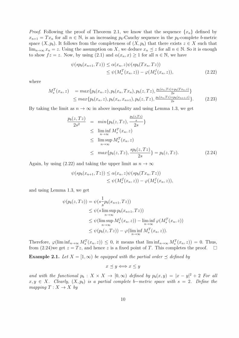
Proof. Following the proof of Theorem 2.1, we know that the sequence {xn} defined byxn+1 = Txn for all n ∈ N, is an increasing pb-Cauchy sequence in the pb-complete b-metricspace (X, pb). It follows from the completeness of (X, pb) that there exists z ∈ X such thatlimn→∞ xn = z. Using the assumption on X, we deduce xn � z for all n ∈ N. So it is enoughto show fz = z. Now, by using (2.1) and α(xn, x) ≥ 1 for all n ∈ N, we have

ψ(spb(xn+1, T z)) ≤ α(xn, z)ψ(spb(Txn, T z))

≤ ψ(MTs (xn, z))− ϕ(M f

s (xn, z)), (2.22)

where

MTs (xn, z) = max{pb(xn, z), pb(xn, Txn), pb(z, Tz), pb(xn,T z)+pb(Txn,z)

2s}

≤ max{pb(xn, z), pb(xn, xn+1), pb(z, Tz), pb(xn,T z)+pb(xn+1,z)2s

}. (2.23)

By taking the limit as n→∞ in above inequality and using Lemma 1.3, we get

pb(z, Tz)

2s2= min{pb(z, Tz),

pb(z,Tz)s

2s}

≤ lim infn→∞

MTs (xn, z)

≤ lim supn→∞

MTs (xn, z)

≤ max{pb(z, Tz),spb(z, Tz)

2s} = pb(z, Tz). (2.24)

Again, by using (2.22) and taking the upper limit as n→∞

ψ(spb(xn+1, T z)) ≤ α(xn, z)ψ(spb(Txn, T z))

≤ ψ(M fs (xn, z))− ϕ(M f

s (xn, z)),

and using Lemma 1.3, we get

ψ(pb(z, Tz)) = ψ(s1

spb(xn+1, T z))

≤ ψ(s lim supn→∞

pb(xn+1, T z))

≤ ψ(lim supn→∞

M fs (xn, z))− lim inf

n→∞ϕ(MT

s (xn, z))

≤ ψ(pb(z, Tz))− ϕ(lim infn→∞

MTs (xn, z)).

Therefore, ϕ(lim infn→∞MTs (xn, z)) ≤ 0, it means that lim infn→∞M

Ts (xn, z)) = 0. Thus,

from (2.24)we get z = Tz, and hence z is a fixed point of T . This completes the proof.

Example 2.1. Let X = [1,∞) be equipped with the partial order � defined by

x � y ⇐⇒ x ≤ y

and with the functional pb : X × X → [0,∞) defined by pb(x, y) = |x − y|2 + 2 For allx, y ∈ X. Clearly, (X, pb) is a partial complete b−metric space with s = 2. Define themapping T : X → X by

10

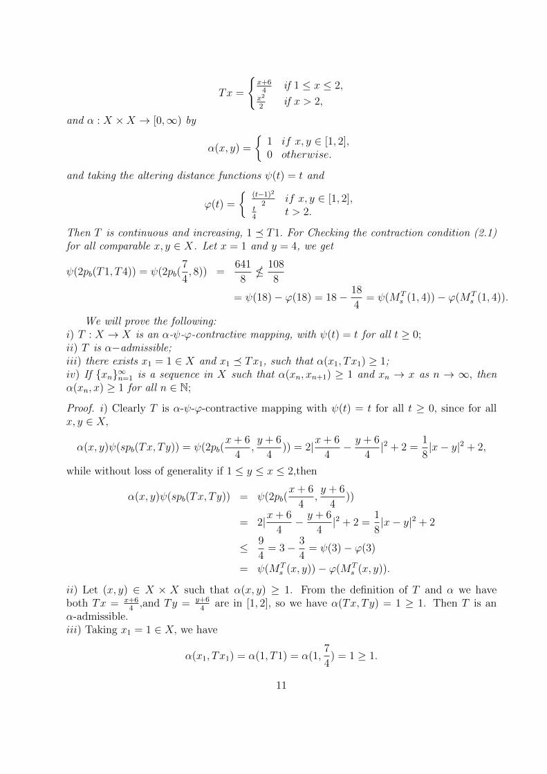
Tx =

{x+64

if 1 ≤ x ≤ 2,x2

2if x > 2,

and α : X ×X → [0,∞) by

α(x, y) =

{1 if x, y ∈ [1, 2],0 otherwise.

and taking the altering distance functions ψ(t) = t and

ϕ(t) =

{(t−1)2

2if x, y ∈ [1, 2],

t4

t > 2.

Then T is continuous and increasing, 1 � T1. For Checking the contraction condition (2.1)for all comparable x, y ∈ X. Let x = 1 and y = 4, we get

ψ(2pb(T1, T4)) = ψ(2pb(7

4, 8)) =

641

8�

108

8

= ψ(18)− ϕ(18) = 18− 18

4= ψ(MT

s (1, 4))− ϕ(MTs (1, 4)).

We will prove the following:i) T : X → X is an α-ψ-ϕ-contractive mapping, with ψ(t) = t for all t ≥ 0;ii) T is α−admissible;iii) there exists x1 = 1 ∈ X and x1 � Tx1, such that α(x1, Tx1) ≥ 1;iv) If {xn}∞n=1 is a sequence in X such that α(xn, xn+1) ≥ 1 and xn → x as n → ∞, thenα(xn, x) ≥ 1 for all n ∈ N;

Proof. i) Clearly T is α-ψ-ϕ-contractive mapping with ψ(t) = t for all t ≥ 0, since for allx, y ∈ X,

α(x, y)ψ(spb(Tx, Ty)) = ψ(2pb(x+ 6

4,y + 6

4)) = 2|x+ 6

4− y + 6

4|2 + 2 =

1

8|x− y|2 + 2,

while without loss of generality if 1 ≤ y ≤ x ≤ 2,then

α(x, y)ψ(spb(Tx, Ty)) = ψ(2pb(x+ 6

4,y + 6

4))

= 2|x+ 6

4− y + 6

4|2 + 2 =

1

8|x− y|2 + 2

≤ 9

4= 3− 3

4= ψ(3)− ϕ(3)

= ψ(MTs (x, y))− ϕ(MT

s (x, y)).

ii) Let (x, y) ∈ X × X such that α(x, y) ≥ 1. From the definition of T and α we haveboth Tx = x+6

4,and Ty = y+6

4are in [1, 2], so we have α(Tx, Ty) = 1 ≥ 1. Then T is an

α-admissible.iii) Taking x1 = 1 ∈ X, we have

α(x1, Tx1) = α(1, T1) = α(1,7

4) = 1 ≥ 1.

11

iv) let {xn} be a sequence in X such that α(xn, xn+1) ≥ 1 for all n ∈ N and xn → x ∈ X asn → ∞. Since α(xn, xn+1) ≥ 1 for all n ∈ N and by the definition of α, we have xn ∈[1,2]for all n ∈ N and x ∈ [1, 2]. Then α(xn, x) = 1 ≥ 1. Now, all the hypothesis of Theorem 2.1are satisfied. Therefore, T has a fixed point.

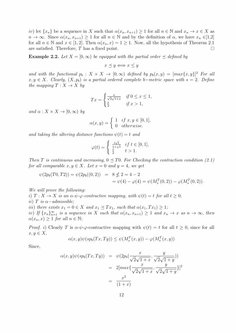
Example 2.2. Let X = [0,∞) be equipped with the partial order � defined by

x � y ⇐⇒ x ≤ y

and with the functional pb : X × X → [0,∞) defined by pb(x, y) = [max{x, y}]2 For allx, y ∈ X. Clearly, (X, pb) is a partial ordered complete b−metric space with s = 2. Definethe mapping T : X → X by

Tx =

{x√

2√1+x

if 0 ≤ x ≤ 1,x2

if x > 1,

and α : X ×X → [0,∞) by

α(x, y) =

{1 if x, y ∈ [0, 1],0 otherwise.

and taking the altering distance functions ψ(t) = t and

ϕ(t) =

{t√t

1+√tif t ∈ [0, 1],

t2

t > 1.

Then T is continuous and increasing, 0 � T0. For Checking the contraction condition (2.1)for all comparable x, y ∈ X. Let x = 0 and y = 4, we get

ψ(2pb(T0, T2)) = ψ(2pb((0, 2)) = 8 � 2 = 4− 2

= ψ(4)− ϕ(4) = ψ(MTs (0, 2))− ϕ(MT

s (0, 2)).

We will prove the following:i) T : X → X is an α-ψ-ϕ-contractive mapping, with ψ(t) = t for all t ≥ 0;ii) T is α−admissible;iii) there exists x1 = 0 ∈ X and x1 � Tx1, such that α(x1, Tx1) ≥ 1;iv) If {xn}∞n=1 is a sequence in X such that α(xn, xn+1) ≥ 1 and xn → x as n → ∞, thenα(xn, x) ≥ 1 for all n ∈ N;

Proof. i) Clearly T is α-ψ-ϕ-contractive mapping with ψ(t) = t for all t ≥ 0, since for allx, y ∈ X,

α(x, y)ψ(spb(Tx, Ty)) ≤ ψ(MTs (x, y))− ϕ(MT

s (x, y))

Since,

α(x, y)ψ(spb(Tx, Ty)) = ψ(2pb(x√

2√

1 + x,

y√2√

1 + y))

= 2[max{ x√2√

1 + x,

y√2√

1 + y}]2

=x2

(1 + x)

12

and

MTs (x, y) = max{x2, x2, y2,

x2 + [max{y, x√2√1+x}]2

4} = x2

Thus

α(x, y)ψ(spb(Tx, Ty)) =x2

(1 + x)≤ x2− x3

1 + x= ψ(x2)−ϕ(x2) = ψ(MT

s (x, y))−ϕ(MTs (x, y)).

ii) Let (x, y) ∈ X ×X such that α(x, y) ≥ 1. From the definition of T and α we have bothTx = x√

2√1+x

,and Ty = y√2√1+y

are in [0, 1], so we have α(Tx, Ty) = 1 ≥ 1. Then T is an

α−admissible.iii) Taking x1 = 0 ∈ X, we have

α(x1, Tx1) = α(0, T0) = α(0, 0) = 1 ≥ 1.

iv) let {xn} be a sequence in X such that α(xn, xn+1) ≥ 1 for all n ∈ N and xn → x ∈ X asn → ∞. Since α(xn, xn+1) ≥ 1 for all n ∈ N and by the definition of α, we have xn ∈[0,1]for all n ∈ N and x ∈ [0, 1]. Then α(xn, x) = 1 ≥ 1.Now, all the hypothesis of Theorem 2.1 are satisfied. Therefore, T has a fixed point

References

[1] T.Abdeljawad, J.Alzabut, A.Mukheimer, Y.Zaidan, “Banach contraction principle forcyclical mappings on partial metric spaces,” Fixed Point Theory and Applications.2012, 2012:154.

[2] T.Abdeljawad, J.Alzabut, A.Mukheimer, Y.Zaidan, “Best Proximity Points For Cycli-cal Contraction Mappings With 0-Boundedly Compact Decompositions,” Journal ofComputational Analysis and Applications. 15(2013), p678.

[3] T.Abdeljawad, “Meir-Keeler α-contractive fixed and common fixed point theorems,”Fixed Point Theory and Applications. 2013, 2013:19.

[4] T.Abdeljawad, E.Karapinar and K. Tas, A generalized contraction principle with con-trol functions on partial metric spaces, 63 (3) (2012), 716-719 .

[5] T.Abdeljawad, “Coupled fixed point theorems for partially contractive type mappings,”Fixed Point Theory and Applications. 2012, 2012:148.

[6] J.Asl, S.Rezapour, N.Shahzad, “On fixed points of α-ψ-contractive multifunctions,”Fixed Point Theory and Applications. 2012, 2012:212.

[7] H.Aydi, M.Bota, E.Karapinar, S.Mitrovic, “A fixed point theorem for set valued quasi-contractions in b-metric spaces,“ Fixed Point Theory and its Applications. (2012).

[8] IA.Bakhtin, “The contraction principle in quasimetric spaces, “Funct. Anal. 30 (1989),26-37.

13

[9] S.Banach, “Sur les operations dans les ensembles abstraits et leur application auxequations integrals, “Fundamenta Mathematicae 3 (1922), 133-181.

[10] S.Czerwik, “Nonlinear set-valued contraction mappings in b-metric spaces,“ Atti Sem.Mat. Fis. Univ. Modena 46 (1998), No. 2, 263-276.

[11] S.Czerwik, “contraction mappings in b-metric spaces, “Acta Math. inform. Univ. Os-rav. 1 (1993), 5-11.

[12] E.Karapinar, R.Agarwal, “A note on Coupled fixed point theorems for α-ψ-contractive-type mappings in partially ordered metric spaces”Fixed Point Theory and Applications.2013, 2013:216.

[13] E.Karapinar, B.Samet “Generalized α-ψ contractive type mappings and related fixedpoint theorems with applications , “Abstract and Applied Analysis (2012).

[14] M.Khan, M.Swaleh, S.Sessa “Fixed pointtheorems by altering distances between thepoints, “Bull. Aust. Math. Soc. 30 (1984), 1-9.

[15] SG.Matthews, “Partal metric topology Proc. 8th Summer Conference on GeneralTopology and Applications, “Ann. N.Y. Acad. Sci. 728 (1994), 183-197.

[16] K.Mehmet, H.Kiziltunc, “On Some Well Known Fixed Point Theorems in b-MetricSpaces.” Turkish Journal of Analysis and Number Theory. 1.1 (2013), 13-16.

[17] Z.Mustafa, et al. “ Some common fixed point result in ordered partal b−metric spaces,“Journal of Inequalities and Applications. (2013), 2013:562.

[18] B.Samet, C.Vetro, P.Vetro, “Fixed point theorems for α-ψ-contactive type mappings,”Nonlinear Analysis. 75(2012), 2154-2165.

[19] S.Shukla, “Partal b−metric spaces and fixed point theorems, “Mediterr. J.Math. (toappear). doi:10.1007/s00009-013-0327-4.

[20] S.Singh, B.Chamola, “Quasi-contractions and approximate fixed points,“ J. Natur.Phys. Sci 16 (2002), No.1-2, 105-107.

[21] H.Yingtaweesittikul, “Suzuki type fixed point for generalized multi-valued mappingsin b-metric spaces, “ Fixed Point Theory and Applications. 23 (2013), 2012:215.

14