@ ( ~ Computer Graphics, Volume 23, Number 3, July 1989

R E N D E R I N G F U R W I T I t T H R E E D I M E N S I O N A L T E X T U R E S

James T. Kajiya Timothy L. Kay

California Inst i tute of Technology Pasadena, Ca. 91125

A b s t r a c t . We present a method for rendering scenes with fine detail via an object called a texel, a rendering primitive inspired by volume den- sities mixed with anisotropic lighting models. This technique solves a long outstanding problem in image synthesis: the rendering of furry surfaces.

I n t r o d u c t i o n

Rendering scenes with very high complexity and a wide range of detai l has long been an important goal for image synthesis. One idea is to introduce a hierarchy of scale, and at each level of scale have a corre- sponding level of detai l in a hierarchy of geometric models (Crow 1982). Thus very complex small objects may have a hierarchy of progressively simplified geometric representations.

However, for very fine detail, a significant problem has so far prevented the inclusion of furry sufaces into synthetic images. The conventional approach gives rise to a severe, intractable aliasing problem. We feel that this aliasing problem arises because geometry is used to define sur- faces at an inappropriate scale. An alternative approacti is to treat fine geometry as texture ra ther than geometry. We explore tha t approach here.

This paper presents a new type of texture map, called a tezel, inspired by the volume density (Blinn 1982). A texel is a 3-dhnensional texture map in which both a surface frame--normal, tangent, and b inormal - - and the parameters of a lighting model are dis tr ibuted freely throughout a volume. A texel is not tied to the geometry of any particular surface. Indeed, it is intended to represent a highly complex collection of surfaces contained within a defined volume. Because of this the rendering t ime of a texel is independent of thegeometr ic complexity of the surfaces tha t it extracts. In fact, wi th texels~ one can dispense with the usual notion of geometric surface models altogether. That is, i t is possible to render texels directly, foregoing referents to any defined surface geometry.

We will use the idea of texels to represent fuzzy surfaces and present an algorithm for rendering such surfaces.

R e v i e w of H i g h C o m p l e x i t y R e n d e r i n g

Many a t tempts to model scenes with very high complexity have been made. One method is to a t tack the problem by brute force computing. A very early effort by Csuri, et al.(1979) generated images of smoke and

Permission to copy without fee all or part of this material is granted provided that the copies are not made or distributed for direct commercial advantage, the ACM copyright notice and the title of the publication and its date appear, and notice is given that copying is by permission of the Association for Computing Machinery. To copy otherwise, or to republish, requires a fee and/or specific permission.

fur with thousands of polygons. More recently, Weil(1986) rendered cloth with thousands of Lambert cylinders. Unfortunately, at a fairly large scale, microscopic geometric surfaces give rise to severe aliasing artifacts tha t overload tradi t ional antialiasing methods. These images tend to look brittle: tha t is, hairs tend to look like spines.

The brute force method fails because the desired detai l should be ren- dered through textures and lighting models rather than through geom- etry. Wha t is desired is the painter's illusion, a suggestion that there is detail in the scene far beyond the resolution of the image. When one examines a painting closely the painter 's illusion falls apart: zoom- ing in on a finely detailed object in a painting reveals only meaningless blotches of color.

The most successful effort to render high complexity scenes are those based on particle systems (Reeves 1983, Reeves and Blan 1985). We believe their success is due in par t to the fact tha t particle systems embody the idea of rendering without geometry. Along the path of the particle system, a lighting model and a frame are used to render pixels directly rather than through a notion of detailed microgeometry. In some sense, this paper represents the extension of particle systems to ray tracing. As the reader will readily discern, even though our rendering algorithm is radically different, particle systems and texels are complementary, e.g. particle systems could be used to generate texel models. Indeed, this paper can be modified to render particle systems in a manner tha t is independent of the number of particles rendered.

Gavin Miller in (Miller 1988) advanced a solution tha t uses a combina- tion of geometry and a sophisticated lighting model much in the spirit of this paper to make images of furry animals. However, like particle sys- tems~ the complexity of the geometric part of his algorithm is dependent on the number of hairs.

The idea of texels is inspired by Blinn's idea for rendering volume densi- ties (Blinn 1982). Blinn presented an algorithm to calculate the appear- aalce of a large collection of microscopic spherical particles uniformly distr ibuted in a plane. This enabled him to synthesize images of clouds and dust and the rings of Saturn. Because Blinn was interested in directionally homogeneous atmospheres, he analytical ly integrated his equations to yield a shnple lighting model.

In Kajiya and Von Herren (1984), Blinn's equations were solved for nonhomogeneous media by direct computation. It was essentially a volume rendering technique for ray tracing. Because our work is based on that earlier effort, we now briefly discuss the relevant equations from Kajiya and Von Herzen (1984}.

As a beam of light travels through a volume of spherical particles, it is scattered and attenuated. The attenuation is dependent on the local density of the volume Mong the ray. The scattering is dependent on the density of the particles scat tering the light and the albedo of each particle. The amount of scattering varies in different directions due to the particle partially occluding scattering in certain directions. This scattered fight then is a t tenuated and rescattered by other particles.

©1989 ACM -0-89791-312 -4/89/007/0271 $00.75

i ~! ~!

i I i i ~ i ̧

'!

:i

)

• i!

i~!i I

21 1 ~I ~i ~

. i i

271

'89, Boston, 31 July-4 August, 1989

This model ignores diffraction around scattering particles.

In ray tracing, we follow light rays from the eye backwards toward the light sources (figure 1). The progressive at tenuat ion along the ray due to occluding particles is computed for each point along a ray emanating from the eye. At each point on the ray through the volume, we measure the amount of light that scatters into the direction toward the eye. This light is then integrated to yield the total light reaching the eye. In this work we use Blinn's low albedo single scatterhxg approximation. That is, we assume that any contribution from multiple scattering is negligible. We assume that the light is scattered jus t once from the light source to the eye. The accuracy of this assumption is relatively good for low albedo particles and suffers as the albedo increases (Blinn 1982~ Rushmeier and Torrance 1987).

Figure 1 shows a schematic of the situation. A volume containing par- ticles with density p(x, y, z) at each point is penetrated by a ray. The light reaching the eye is computed along the ray R. At each point P = (x(t), y(t),z(t)) of the ray at distance t, the i l lumination Ii for each light source is multiplied by a phase factor p(cos 0) that indicates how much of the light is scattered from the light source to the ray. The brightness is then weighted by the density p of the particles at this point. The attenuation between point P and A due to the medium is given by an integral of the density along the ray. The equations are:

and

× p(~(t), y(t / , . ( t / ) dt

(1)

(2)

Equation 1 calculates the transparency T of the density p. It says that tha t each small distance ds along a ray multiplicatively accumulates the transmission coefficient by e -rpd~. The coefficient r converts the density of the particles into an at tenuat ion coefficient. The quantities tne~,tfa~ are the near and far distances of the density that contribute to the calculation.

Equation 2 calculates the brightness B by integrating the brightness of each piece dt along the ray (x(t), y(t) ,z( t)) according to three fac- tors. The first factor introduces the at tenuation of the medium Mong the ray into the surface. Bright particles buried deep within a density are occluded by many particles, thus the accumulated transmission co- efficient is low and the particle will not contribute much light to the pixel. Note tha t this factor is calculated as in equation 1. The second factor multiplies the il lumination I i for each light source i reaching the particle (which is given as a transmission as in equation 1), times the lighting model for each single particle, this is given by the phase factor p(cos0). This phase factor is a function of the angle 0 between the light direction and the eye direction. It represents the amount of occlusion of the scattered light and is much like the phase of the moon. The third factor weights the brightness by the density of particles at a given point. A few bright particles will contribute less light than a large number of dimmer particles.

Calculating the illumination component I~ can be done in many ways. Blinn (1982) assumed a homogeneous field and calculated the trans- parency of the medium from point P to point C~ for each light source (figure 1). Kajiya and Von Herzen (1984) assumed an infinite distance (viz. collimated) light source and precalculated the intensities for each point in the volume by marching along a parallel wavefront. Rushmeier and Torrance (1987) solve a system of linear equations to yield Ii.

Following Blinn(1982), many workers have expanded on the volume density theme: Voss(1983), Max(1983), Kajiya and Von Herzen(1984), Max(1986b, 1986e), Rushmeier and Torrance(1987), and Nishita, Miyawaki and Nakamae(1987). These algorithms extended Blinn's orig- inal work to rendering densities with nonuniform distribution, to high

albedo solutions, and to more general geometries. Rushmeier and Tor- rance(1987) represents the most sophisticated effort to date, calculating a physically accurate distribution of light for true multiple sca t te r ing-- albeit with isotropic scattering models.

The recent popularity of scientific visualization has engcndered much re- cent activity in volume rendering, e.g. Sabella(1988), Upson and Keeler (1988), Drebin, Carpenter, and Hanrahan(1988). The technique out- lined in this paper has direct application to the volume rendering of vector fields. In particular, one result of this work has part icular rele- vance to volume rendering: the hnportance of shadows. In the results section, we have rendered an identical texel with and without shadows. As the pair of torii in figures 10 and 11 show, rendering without taking into account shadows creates a situation that is so unphysical that the data cannot be properly interpreted by our visual system.

We also point out that the technique presented in this paper fits well into the ray t racing/distr ibuted ray tracing/rendering equation framework. That is, texels can be mixed with the wide variety of primitives already amenable to ray tracing. It is not clear whether texels can be made compatible with the radiosity approach to image synthesis.

Texels

In Kajiya and Von Herzeu(1984) it was suggested that volume densities were potentially capable of rendering many complex objects beyond particles of dust and smoke: this would include phenomena such as hair and furry surfaces. We began this work a t tempt ing to generalize volume density rendering along these lines. During the course of the investigation, we found that the idea of using volume densities to model surfaces is not entirely appropriate. Although the idea of distr ibuting lighting models instead of spherical particles within the volume density is the right idea, we have found that one cannot not s imply replace particle lighting models with surface lighting models. The physics of scattering from surfaces is so different from that of particles that new equations governing the rendering process must be derived.

To generalize volume densities we now introduce texels. In practical terms, a texel is a three dimensional array of parameters approximating visual properties of a collection of microsurfaces. If texels are to be used to replace g e o m e t r y ~ u c h as trees on the side of a moun ta in - - then the microsurfaces of leaves and branches will be stored into the volume array. At each point in space, several items must be stored. First is the density of microsurfaces. That at certain points, space is empty; at others, there is a dense array of leaves. A second item distributed throughout space is a lighting model. In a texel, each leaf is not stored as a polygon. Instead the collection of leaves is represented by a scattering function tha t models how light is scattered from the aggregate collection of surfaces contained within a volume cell. This scattering function is represented by a pair of quantities, the first is a frame, that is a representative orientation of a microsurface within the cell, and a reflectance function.

Texels may be generated many different ways. We have not investigated techniques for generating texels for many interesting cases. For example, the geometry for the trees could be sampled into three~:limensional arrays using some sort three-dimensional scan-conversion technique. We have not done thisj however. For representing fur~ the generation of texels is straightforward and is presented in a section below.

Texels are intended to simulate a volume cell that contains bits of sur- faces, not spherical particles. Thus the first component of a texel is a scalar density p which represents not relative volume, but an approxi- mation to relative projected area of the microsurfaces contained within a volume cell. The second component of a texel is a field of frames B, that is the local orientation of the mlcrosurface within a volume cell. The third component is a field of lighting models ~, which determine how light scatters from this bit of surface.

Def in i t i on . A texel is a triple p ,B, g, consisting of a scalar density p(x,y,z), a frame bundle B = [n(x,y ,z) , t (x ,y ,z) ,b(x ,y ,z)] , and a

272

~/~ Computer Graphics, Volume 23, Number 3, July 1989

field of bidirectional l ight reflection functions

~ (~ ,y ,~ ,0 ,¢ ,¢ ) .

The scalar density p measures how much of the projected unit area of a volume cell is covered by microsurfaces. It should properly be a higher tensor quanti ty that takes into account the viewing vector, but we adopt the approximation that this quanti ty is an isotropic quanti ty and hence a scalar.

The frame bundle B indicates the local orient ation of the surfaces within the texel. It is a field of coordinate basis vectors n~t~b that are called the normal, tangent, and binormal fields, resp.

The bidirectional light reflection function • indicates the type of surface contained therein. It is possible to combine B and • into a single anisotropic lighting model field, but we have separated them because, often, either component may be taken to be constant throughout the volume while the other varies.

Texels appear to be a na tura l extension of a volume density. Because in a volume density the spheres are physically and materially isotropic, the frame and reflectance fields are homogeneous. Thus they do not need to be distr ibuted throughout a density but can be established as single quantities. Texels simply generalize this a bit.

l ~ e n d e r i n g Texe l s

How can one modify volume densities to model hair? A naive approach would be to simply reinterpret the density p to reflect the densities of the hair at each volume celt; and to modify the lighting model at each point to correspond to scattering from a cylinder instead of a sphere. Unfortunately this direct approach~ while correct in spirit, has flaws.

For an insight into understanding why volume densities are not appro- priate for rendering microsurfaces~ consider the rendering of a single plane surface via a volume density (figure 2). Assume tha t the surface is stored into a volume density so tha t it bisects the cube. The optical depth of the surface is so high that it simulates an opaque surface, Let the phase factor of the particle lighting model be say a Lambert ian sur- face lighting model in equations 1 and 2. Let us not use equations 1 and 2 to calculate both the transparency and the brightness of the surface.

For the transparency calculation, even though the optical depth param- eter ~ is set very high, the line integral of the density in the exponent will be vanishingly small. This is because the surface is infinitely thin~ so the line integral will pierce the surface at only a single point. This yeilds an integral Of 0.

A similar problem occurs in the brightness calculation. The brightness integrand yields a finite value whose contribution to the integral along the ray will be zero, since it is nonzero only for a single point.

Thus the transparency and brightness for this surface will both be zero-- an invisible surface! Obviously, volume rendering needs to be modified somewhat to be able to render surfaces. The problem is tha t the relative volume of mierosurfaces does not determine brightness and opacity for surfaces as it does for point particle densities. A single surface with zero volume can be completely opaque and can reflect 100% of its incident light. Yet its relative volume will be zero. Thus, what is called for is something like a density which is given by Dirac delta functions. This, along with a more general lighting model, is the essence of the texel idea.

Texels are rendered in a manner which is similar to tha t for volume densities, suitably generalized. Again, the equations model the si tuation schematized in figure 1. The texel containing surfaces with projected area density p(z, y,z) at each point is penetrated by a ray. The light reaching the eye is computed along the ray R. At each point P = (x(t),y(t),z(t)) of the ray at distance t, the i l lumination h for each light source is multiplied by the bidirectional reflectance function gt tha t indicates how much light is scattered from the light source to the

ray. The brightness is then weighted by the projected area density at this point. The attenuation between point P and A due to the medium is given by an sum of the density along the ray.

The equations for a texel i l lumination are

T = , - " E :~L . . r ~(~(,),v(,),~(,)) (3)

and

B = tfar

t--tnear

×[~Ii(x(t),Y(t),z(t))ff2(x(t),y(t),z(t),O,¢,P)]

× 0(=(t), y ( t l , . ( t ) )

(4)

Equations 3 and 4 are similar to equations 1 and 2. Equation 3 is just equation 1 with the line integral replaced by a sum. We write the sum because integrating Dirac del ta functions on microsurfaces sums the contribution at each microsurface.

In equation 4, the relationship to equation 2 is also evident. The inte- gral has again been replaced by a sum. The at tenuation along the ray segment AP in figure 1 is represented by the first term in the product. The second term models the scattering of light from the microsnrface. As in equation 1 there is a te rm for eacl~ light source. The illumina- tion I¢ reaching the microsnrface is multiplied by the bidirectional light reflection function • of the microsurface. Finally, the projected area density scales the reflected l ight in the third term.

The transmission equation 3 for texels is a formal sum instead of an integral. This formal sum is taken over each of the surfaces in the density along the ray. If this sum is infinite, then the transmission coefficient is zero, indicating that the density is totally opaque. The brightness equation 4 is also a formal sum instead of an integral. This is because, a t each surface intersecting a ray, we are adding the brightness contribution of the surface at that point.

It would appear tha t equation 4 would always yield an infinite quantity, but recall that the terms of the formal sum will be zero where there are no surfaces and behind any surface the optical depth will be high and will a t tenuate all contributions to zero. Thus the sums are finite.

Calculation of the incident intensities I~ are computed by using equation 1 reeursively. That is, a ray is shot from the point P to each light source i (figure 1). The transmission coefficient is calculated from equation 1. The intensity I~ is simply the brightness of the light source at tenuated by the transmission coefficient along the segment PC~.

The algorithm just outlined would be impossibly expensive if the sums were to be evaluated by adding terms corresponding to every point along the original ray. The algorithm presented in the next section approxi- mates these sums by a Monte Carlo t reatment tha t computes expected values of random samples along the ray, in the spirit of distributed ray tracing (Cook, et al. 1984).

Texe l R e n d e r i n g A l g o r i t h m

The texel rendering algorithm computes the above sums by approxi- mating them with with expected values of random samples along the ray. To find the intensity of light emanating backwards from a given ray, the intersection of the ray and each texel boundary is calculated. The distances along the ray of these intersections then forms an interval from tnear to t.far along the ray, shown as point A and D of figure 1. To compute the sum, we use the technique known as stratified sampling. We divide up the ray into a series of segments (delineated by tick marks along the ray in figure 1). In each segment a random point is chosen to calculate the scattering term, e.g. point P. The il lumination Ii is calcu- lated by recursively shooting a ray toward each light source as discussed

273 ;i

'89, Boston, 31 July-4 August, 1989

274

in the previous section. Finally the sum over segments are calculated to approximate the quantities in equations 3 and 4.

1. Intersect a ray with the all texel boundaries to find tnear , ~far for each texel. Sort all intersections frora front to back and match with distance. Let Tnear ~ min ~near where the minimum is over all segments. Similarly Tfar = m a x ~far.

2. Divide up the ray from Tnear to Tfa r into ray segments ~i of length L, where 1 is a reference length parameter, the number of sexnples per unit distance in world coordinates set by the user. (The last segment may be shorter than L).

3. Set transparency to unity.

4. FOIl. each segment.

4.1 Shoot shadow rays from the sa*nple toward every light source to calculate the amount of light reaclfin s tiffs point.

4.2 Calculate b~ightness from li~shting model and illumination intensity and multiply by transparency to give overall brightness contribution to the pixelpiffel = pixel + trans * lightblodel.

4.3 Multiply transparency by e to, the transmission coefficient of the

segment.

5. At the end segment, calculate brightness as above but normalize by fractional

length of the segr~¢nt.

Step 5 in the algorithm above is required to avoid bias in the Monte Carlo calculation. If the final segment were to be treated as a full length section then the averages would be thrown off. This has an effect of making the edges of the volume appear slightly more opaque than they should be.

This section presents an algorithm for rendering a single texel. However, to make pictures of fuzzy objects, four steps must be carried out. These are the creation of the texels, the mapping of texels into world space, the intersection of rays with texels, and the computation of the lighting model.

G e n e r a t i n g Texe ls fo r H a i r

We will now direct our attention to methods for generating texels that represent patches of hair. The general problem involves long flowing hair. Particle systems could be used to trace the trajectories of the individual hairs through a three-dimenslonal array. The particle would leave an ~anti-aliased" trail of density that would be summed in with previous densities.

A texel representing hair may be simplified by storing only the density p and the frame B at each point. The bidirectional reflectance function

is constant for each hair and common to all hairs (if the hair does not change color). Thus it is not necessary to store it throughout the volume. For the lighting model derivation we t reat an individual hair as an infinitely thin cylindrical surface. Thus, the only element of the frame that is necessary is the tangent vector along the hair. The rest of the frame B, normal and binormal, do not enter into the lighting calculations and were omitted. Thus a particle system generating hair would not only leave a track of density but also store a tangent vector representing the direction of the velocity of the particle.

The teddy bear model presented in this paper uses a single texel repli- cated over the bear 's skin. The contents of the texel were generated using a much simplified version of the particle system approach. All hairs on the teddy bear are straight lines that point in the same direc- tion, perpendicular to the scalp (in texel space). This implies that the hairs will lie along an axis 6f the three-dimensional array used to store the texel. Thus the tangent vectors are all the same in that they all perpendicular to the scalp. Thus they were also excluded from volume structure.

The bear 's fur texel was stored as a 40x40xl0 array. The contents of the array were designed based on several criteria:

1. The "hairs" axe distributed as a Poisson disk.

2. The Poisson disk is created with a torus topology, so the single texel can tile

tim entire bears surface without showing seams.

3. Animal fur often comes in two layers, an "overcoat," and an "undercoat." The undercoat is a dense cover of short fur, while the overcoat is a sparser distribution of long hair. We have found this to be an important feature for avoiding a brushlike appearance.

A "modeling" program allowed us to search the parameter space and presented us with top and side projections of the texel. Using purely aesthetic (and largely arbitrary) judgement, the texel used in figures 15 azld 16 was created.

M a p p i n g Texe l To W o r l d S p a c e

By placing texels over the surface of the bear, we created a bear whose fur flows smoothly over its entire body, while at the same time shows local randomness. However, a texel representcd as a three-dlmensional array, is shaped as a rectangular sohd, at least in texel space. The texels must be mapped onto the shape of the bear in a continuous way to avoid gaps.

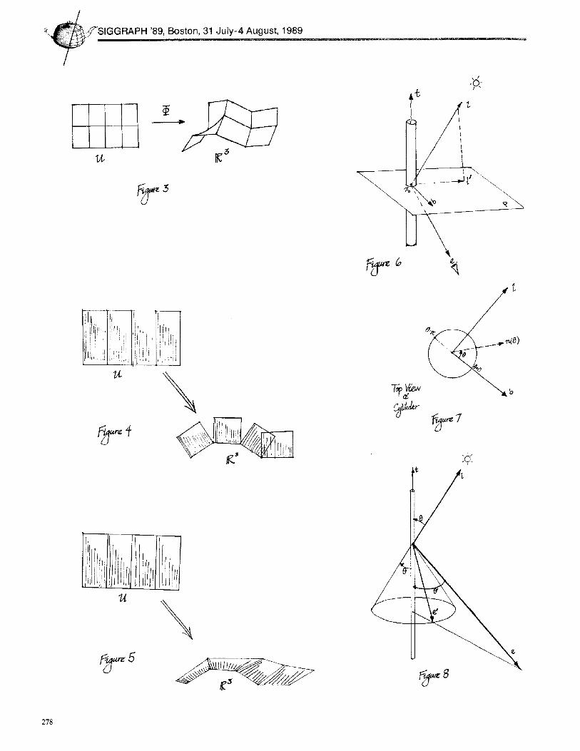
The teddy bear was modeled using a new technique called generative models. Each body part (head, body, ear, arm, leg, and nose) was constructed by designing a parametric mapping (I' from a rectangle U (parameterized by u and v) into world space R 3. If we were to render the bear as polygons (as we do in the case of the bear 's nose), we would chop the rectangle into a mesh of n x m small squares. Each square would be mapped vertex by vertex through if9 into world space. The resulting objects (bihnear patches) would then be rendered (usually by further approximating each patch as two triangles). Figure 3 demonstrates this approach. For the sake of simplicity, all figures will present just two dimensions when possible. The extension to three dimensions is obvious.

The texel cubes are mapped into world space in exactly the same way. The parameterized rectangle is chopped into n × m small squares. Each square is mapped into world space and is identified with the base of a texel (figure 4). (In the case of the teddy bear, a single texel was replicated over the entire surface of the bear.)

The mapping q) defined by the generative modeling specifies what hap- pens only to the base of each texel; The texel's third dimension (height) must also be mapped into world space. This mapping specifies ff the fur on the bear stands straight out or if it lies down. The extension of 4) to the third texel dimension need only be defined for the corners of the texel. Once the corners of the texels are mapped, they are no longer necessarily boxes. Additionally, the gaps between adjacent texels dis- appear (figure 5). The hnear nature of the texel interpolation described in a following sections assures that the hairs within a texel will flow in the same general direction as the corners.

A modeling program was created tha t allowed the designers to manipu- late the orientation of the corners of the texels. The program starts with the corners of each texel sticking straight out (i.e., the corners of each texel correspond with the surface no rman of the scalp). The corners are then perturbed by global Fourier maps.

I n t e r s e c t i n g R a y s W i t h Texels

A texel is shaped as a rectangular solid in texel space. The mapping of the texel into world space as described above changes each of the six faces of the rectangular solid into a bihnear patch. The intersection of a ray with a texel is accomplished by intersecting the ray with the six faces of the texel in world space.

Intersecting Rays with Bilinear Patches

Each edge of a bilinear patch, as well as all "horizontal" and "vertical" cross sections on the patch are straight lines. All other cross sections of a bihnear patch are quadratics. Therefore, it seems reasonable that the ray-patch intersection calculation should involve solving the quadratic equation.

~ Computer Graphics, Volume 23, Number 3, July 1989

A ray is defined by the equation R = at + b with 0 <_ t. The 3-vectors a and b specify the origin and direction cosines of the ray. A bilinear patch is of the form P - ~ A u v + B u + C v + D with 0 _< u < 1 and 0 < v < 1 where A, B, C, and D are also triples.

The intersection of the ray R with the patch P occurs when R = /9. Expanding into components yields three equations of the form,

A l u v + B l u + Clv + D l t + El = 0, (5a)

A2uv + B2u + C2v + D2t + E2 = 0, (5b)

and A3uv + B3u + Czv + D3t + E3 = 0. (5c)

These equations should be reordered so tha t the first is the one with the largest D coefficient. This will assure that, in the case of a patch aligned with an axis~ the denominators in the equations that follow will be reasonable (thereby avoiding floating point overflows).

The first equation is solved for t, yielding

A~uv + B=u + C~v + E~ t = D= ' (6)

which can be subst i tu ted into the remaining two equations to remove references to t, result ing in two equations of the form

F2uv + G2u + H2v + / 2 = 0 (7a)

and Fsuv + G n u + Hsv + Is = 0. (7b)

These two equations can be multiplied by Fs and F2 respeetivelyj and the uv term can be eliminated, giving a linear equation relating u and v. Solving for u and backsubsti tut ing into equation (7a) or (7b) results in a quadratic equation in v. Once v is determined, u quickly follows, as does t.

When solving the quadratic equation (of the form ax e + bz + c = 0), there is a possibility tha t the coefficient on the square term (a) may be very small. This could occur, for example, when the four points of the bilinear patch are coplanar. Since we are looking only for values of 0 _< u < 1, we can compute if a is too small using the equation

b + sgn(b)X/V - 4ac < 2a. (8)

If the equation falls to hold, then the root would be out of the range - 1 < u < 1, and need not be computed. This and similar tests will help avoid floating point overflows.

M a p p i n g R a y - T e x e l I n t e r s e c t i o n s t o Texe l Space

Once the intersections of the ray with the texel have been computed, they must be mapped into texel space. Then the texel properties (such as density and tangent vector) can be found by trilineax interpolation from the texel arrays.

To compute the mapping, all the intersections are sorted. Ideally, they will come in pairs, the first of the pair (anear ' ) representing the ray en- tering the texel, and the second (afar,) representing the ray leaving the texel. The intersections yield pairs of the form (fn . . . . u . . . . . v . . . . . tnear) and (flat, tafar,°far~tfar), where f is the index of the face intersected, (u, v) is the patch coordinate for the intersection in face f, and t is the distance along the ray for the intersection.

Each intersection is mapped back to the texel in texel space, resulting in points of the form (z . . . . . Yn . . . . Z . . . . . t . . . . ) and (zf~, Yfar, Zfar,tfar), where (z, y, z) is the coordinate withing the unit texel of the intersection. The t values remain unchanged.

The (x, y, z) coordinates of an intersection in texel space will fall in the unit cube. At least one of the components will actually be either 0 or 1, except when an intersection happens for t < 0. In this case, the (x, y, z)

coordinates of the intersection must be adjusted by interpolation to match the point on the ray where t -- 0.

To render the scene, the shader must know the value of the texel at many points along the ray. Because the t parameter is invariant under the texel-space-to-world-space mapping, we can use it as the interpolant to compute the texel space coordinate for any value of t. The three components are

and

t -- tnear - - - - ~ - ( x f ~ - - z . . . . ) + z . . . . . Har --~near

t - t ..... ( y f ~ r - y . . . . ) + v . . . . . .

tfa r -- tnear

t - t . . . . (Zf~r - Z . . . . ) + z . . . . . . tfa r ~ tnear

L i g h t i n g m o d e l for h a i r

(9a)

(gb)

There are two components forming the lighting model for a single hair, the diffuse and specular. The diffuse component is derived essentially from the Lambert shading model applied to a very small cylinder. The specular component is an ad hoc model similar to the Phong light re- flection model that has been modified for cylindrical surfaces.

A more rigorous approach to defining a lighting model would be some- thing along the lines of Kajiya (1985), of Cabral, Max, and Springmeyer (1987), or of Krueger (1988). These papers propose algorithms to con- vert the the surface microgeometry to be represented in the volume directly to lighting models. We have found, however, the exact form of the details of the lighting model not to be particularly critical to the quali ty of the images. Examination of the images show tha t our ad hoc approach is adequate.

The geometry for deriving the hair lighting model is shown in figure 6. An individual hair is a line segment specified by a position x0 and a tangent vector t. The light vector I points from Xo to the light source. The eye vector e indicates the direction of the scattered light toward the eye. All of these vectors are assumed to be of unit length. The projection I I of 1 onto the plane perpendicular to t forms the second basis vector. The third basis vector b is chosen to be perpendicular to both the previous basis vectors.

The diffuse component

The diffuse component of the hair reflection model is obtained by in- tegrating a Lambert surface model along the circumference of the half cylinder facing the light source. As shown in figure 7, we integrate over the half circle visible from the light source. The back of the surface is not il/umlnated. The orthonormal basis formed from the three vectors t~l', b are easily calculated. The first basis vector is t, which is perpen- diculax to the texel base. The second vector E is the projection of the light vector l onto plane P containing all the normMs to the cylinder. The vector l t is given by

r = z - (t . 1)t (lO) IIz - ( t . z)ttl "

It is easy to see that b, orthogonal to t and l ~ is calculated as

b = l × t . (11)

These three vectors are shown in figure 6.

The total amount of light scattered per unit length of cylinder is inte- grated over the semicircle from shadow terminator to shadow termina- tor (figure 7). Let us parameterize the position along the cylinder by 0 where 0 ranges between 0 and ~r radians. As a function of 0 the normal vector n to the cylinder is

= b(cos0) + V(sin o). (12)

275

'89, Boston, 31 July-4 August, 1989

!i :

!i?i ~ 276

The Lambert model gives the intensity of reflected l ight as ~(~) = (kd)l. n, where /ca is the diffuse reflection coefficient. Thus to find the total amount of light per unit length we integrate along the circumference of the half cylinder. The line integral element ds along the cylinder is given in terms of 8 by r dO, so

// ~dif]use = hd l" n r dO

f/ = ke r Z. (b(cosO) + l ' (s in 0)) dO ( la)

f/ = kd r l . l ' sinOdO

= ( g d ) l . l'

where Kd absorbs all the quantit ies independent of l and l ~. Substitut- ing the definition of l ~ into the definition yields a part icularly simple expression for the diffuse component:

l - ( t . l)t ~a,.rf~,~ = K,~ l lit - ( t Otll

= Kd 1 - ( t . l ) 2 (14)

= Kd sin(t , l) .

Thus the diffuse fighting component is proportional to the sine between the light and tangent vectors. Thus if the tangent of the hair is pointing straight at the fight, the hair is dark. This is readily observed in real hair.

The specular component

Calculating the highlights on a hair requires some term capturing spec- ularity. We could have derived a specular term in a similar manner s tar t ing from the ad hoe Phong specular model. However, the process is more difficult and the result ing model quite complex. We chose in- stead to invent an ad hoc specular model in the same spirit as the Phong model modified to approxlmat~ some diffraction around the hair. The model is motivated by figure 8.

Any light striking the hair is speeularly reflected at a mirror angle along the tangent. Since the normals on the cylinders point in all directions perpendicular to the tangent, the reflected light should be independent of the azimuthal component of the eye vector. Thus the reflected light

.forms the cone whose angle at the apex is equal to the angle of incidence as shown in figure 8. The actual highlight intensity is given as

• , p o , , , , = k, cos~(e, e') (15)

where k, is some specular refect ion coefficient, e is the vector pointing to the eye, and e n is the specular reflection vector contained in the cone closest to the eye vector, and p is the Phong exponent specifying the sharpness of the highlight. The highlight is thus a maximum when the eye vector is contained in the reflected cone and falls off v~ith a Phong dependence.

To calculate this model we note that the only quanti t ies entering into the calculation are the angle of incidence and the angle of reflection with respect to the tangent vector, 0 and 0 ~. The intensity is given by

~]TA/ap¢cula r ~ ha COSP 0 - - OI

= hdcose cos0' + sin0 sine'), (16)

= h , ( t . 1 t s + sin(t , l) einCt, e))~

These quantit ies are easily calculated from the original vectors.

R e s u l t s

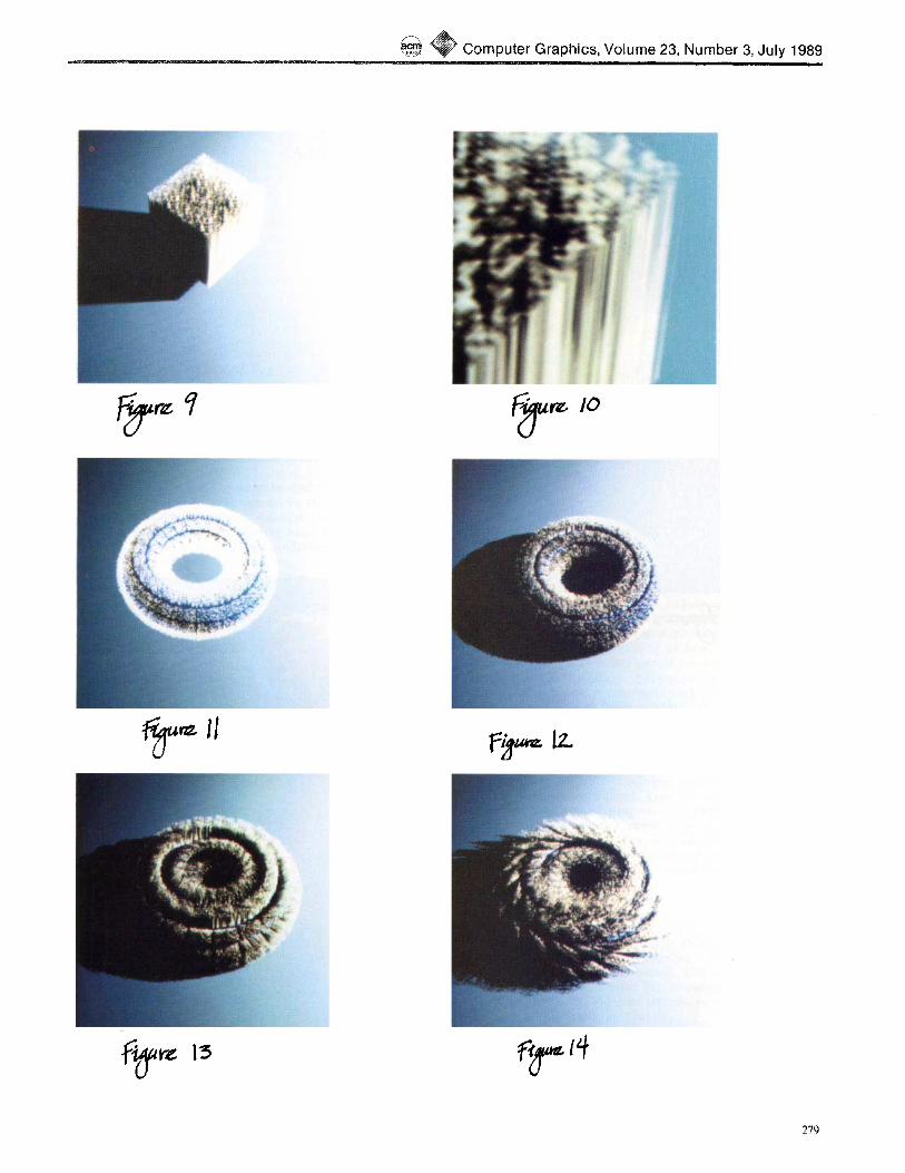
Figure 9 shows a single texel of hair. Discounting the base plane, no geometric model has been used to create this image. Figure 10 shows

a closer view of the r ightmost edge of figure 9. Note tha t the painter 's illusion breaks down on the close up view. We should switch from the texel representation to actual geometry when viewing the model at this resolution.

Figures 11, 12, 13 and 14 show a number test images displaying torli covered by texels, modeling brushlike fur. These show what happens when the corners of the texels are not deformed by ¢.

Figures 11 and 12 are identical except tha t figure t l was rendered with the shadows turned off, so that every cell is always i l luminated. It is evident that self shadowing of the texel is one of the principal cues for realism.

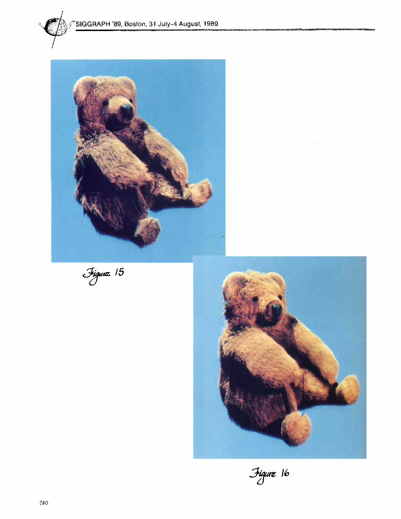
Figures 15 and 16 show two versions of a teddy bear. The underlying geometric model is identical for each bear. Different Fourier coefficients were used for defining each local texel deformation. Fewer, larger texels appear in figure 15. The processor time for each of these images was substantially the same. These images have a resolution of 1280 by 1024 pixels. No antialiasing was done.

Precise measurements of the CPU time are somewhat problematic, as each image was rendered concurrently on a network of large IBM main- frames. We used a total of twelve 3090 processors and four 3081 pro- cessors. On average, we obtained approximately 30%-50% of each pro- cessor. Total wall clock t ime was about 2 hours.

F u r t h e r W o r k

The question of how to turn geometry into texture has not yet been solved. Thi~ paper represents only a start on the problem. An auto- matic way of generating texel densities from complex geometric models is currently unknown to us. We speculate tha t the theory known as geometric measure theory may provide the key mathemat ica l insights into this problem.

Applying texels to other complex scenes is also left open: consider the problem of rendering a forest covering a mountainside in the distance. Instead of having thousands of polygons, each tree and bush could be modeled as an appropriate texel. When the texels themselves become very small, one can merge several into a larger texel, somehow adding densities and merging lighting functions.

We have not modeled long hair, or curly hair; only fur. This is an interesting modeling task especially when one decides to include the dynamical behavior of long hair in an animation. We believe tha t the methods presented in this paper will adequately render long hair once the modeling problems are solved.

R e f e r e n c e s

Blinn J.F. and Newell M.E. (1976) "Texture and Reflection in Computer Generated Images" Comm. ACM 19,10, 542-547.

Blinn J.F. (1977) "Models of Light Reflection for Computer Synthesized Pic- tures" Computer Graphics 11,2, 192-198.

BIinn J.F. (1978) "Simulation of Wrinkled Surfaces" Computer Graphics 12,3, 286-292

Blinn J.F. (1982) "Light Reflection Functions for Simulation of Clouds and Dusty Surfaces" Computer Graphics 16,3, 21-29.

Cabral B., Max N. and Springmeyer R. (1987) "Bidirectional Reflectance Functions from Surface Bump Maps" Computer Graphics 21,4, 273-282.

Catmull E.E. (1974) A Subdivision Algorithm for Computer Display of Curved Surfaces, Ph.D., U. of Utah.

Cook R.L., Porter T. and Carpenter L. (1984) "Distributed Ray Tracing" Computer Graphics 18,3, 137-146.

~ Computer Graphics, Volume 23, Number 3, July 1989

Cook R.L. (1984) "Shade Trees" Computer Graphics 18,3, 223-232.

Crow F.C. (1982) "A More Flexible image Generation Environment", Com- puter Graphics 16,3, 9-18.

Csuri C., Hakathorn R., Parent R., Carlson W. and Howard M. (1979) "To- wards an interactive high visual complexity animation system" Computer Graphics 13,2, 289-299.

Drebin R.A., Carpenter L., and Hanrahan P. (1988) "Volume Rendering", Computer Graphics 22,4, 65-74

Kajiya J.T. and Von Herzen B. (1984) "Ray Tracing Volume Densities" Com- puter Graphics 18,3, 165-174.

Kajiya J.T. (1985) "Anisotropie Reflection Models" Computer Graphics 19,3, 15-22.

Krueger W. (1988) "Intensity Fluctuations and Natural Texturing" Computer Graphics 22,4, 213 220.

Miller G.S.P. (1988) "The Motion Dynamics of Snakes and Worms" Computer Graphics 22,4, 169-178.

Max N.L. (1986a) "Light Diffusion through Clouds and Haze" Computer Vi- sion, Graphics and Image Processing 33,280-292.

Max N.L. (1986b) "Atmospheric Illumination and Shadows" Computer Graphics 20,4, 117-124.

Max N.L. (1986e) "Shadows for Bump Mapped Surfaces" in Advanced Com- puter Graphics, Springer V., 145-156.

Nishita T., Okamura I. and Nakamae E. (1985) "Shading Models for Point and Linear Sources" ACM Trans. on Graphics 4,2, 124-146.

Nishita T., Miyawaki Y. and Nakamae E. (1987) "A Shading Model for At- mospheric Scattering Considering Luminous Intensity Distribution of Light Sources" Computer Graphics 21,4, 303-310.

Ohira T. (1983) "A Shading Model for Anisotropic Reflection" Tech. Rep. Inst. El. and Comm. Eng of Japan (in Japanese) 82,235, 47-54.

Peachey D.R (1985) "Solid Texturing of Complex Surfaces" Computer Graph- ics 19,3,279-286.

Perlin K. (1985) "An Image Synthesizer" Computer Graphics 19,3, 287-296.

Reeves W.T. (1983) "Particle Systems--A Technique for Modefing a Class of Fuzzy Objects" Computer Graphics 17,3, 359-376.

Reeves. W,T. and Blau R. (1985) "Approximate and Probabilistic Algorithms for Shading and Rendering Structured Particle Systems" Computer Graphics 19~3, 313-322.

Rushmeier H.E. and Torrance K.E. (1987) "The Zonal Method for Calculat- ing Light Intensities in the Presence of a Participating Medium" Computer Graphics 21,4, 293-302.

Sabella P. (1988) "A Rendering Algorithm for Visualizing 3D Scalar Fields", Computer Graphics 22,4, 51-58.

Takagi J., Yokoi S. and Tsuroka S. (1983) "Comment on the Anisotropic Reflection Model" Bull. of SIG. Graphics and CAD, Inf. Proc. Soc. of Japan. (in Japanese) l l ,1 , 1-9.

Upson C., Keeler M. (1988) "VBUFFER: Visible Volume Rendering", Com- puter Graphics 22,4, 59-64.

Acknowledgments

Thanks to A1 Barr for technical discussions, and to Hewlett Packard Corpo- ration for their donation of the HP9000 Model 350SRX workstations to the Caltech Computer Science Graphics Lab.

Our appreciation to John Snyder for modeling and remodeling (and reremod- chug) the bear,

We wish to express our thanks to IBM and Alan Norton of IBM T.J. Watson Research Center at Yorktown Heights their financial support and gracious donation of a considerable amount of 3090 time,

We also th~nk the reviewers whose many comments have been invaluable in improving our exposition.

\ f / \

-ur~ L

j¢/ !

¢t \ \

I l

277

'89, Boston, 31 July-4 August, 1989

+.

72

~ 8

278

~ Computer Graphics, Volume 23, Number 3, July 1989

7ff,~ q

279

~ii ill

'89, Boston, 31 July-4 August, 1989

!i I

ii! 280

,,r~ 15