.

Computational GenomicsLecture #2

This class has been edited from Nir Friedman’s lecture which is available at www.cs.huji.ac.il/~nir. Changes made by Dan Geiger, then Shlomo Moran, and finally Benny Chor.

Background Readings: Chapters 2.5, 2.7 in Biological Sequence Analysis, Durbin et al., 2001.Chapters 3.5.1- 3.5.3, 3.6.2 in Introduction to Computational Molecular Biology, Setubal and Meidanis, 1997.Chapter 11 in Algorithms on Strings, Trees, and Sequences, Gusfield, 1997.

1. Hirshberg linear space alignment 2. Local alignment3. Heuristic alignment: FASTA and BLAST4. Intro to ML and Scoring functions

2

Global Alignment (reminder)

Last time we saw a dynamic programming algorithmto solve global alignment,whose performance is

Space: O(mn)Time: O(mn) Filling the matrix O(mn) Backtrace O(m+n)

Reducing time to o(mn) is a major open problem

0A1

G2

C3

0 0 -2 -4 -6

A 1 -2 1 -1 -3

A 2 -4 -1 0 -2

A 3 -6 -3 -2 -1

C 4 -8 -5 -4 -1

ST

3

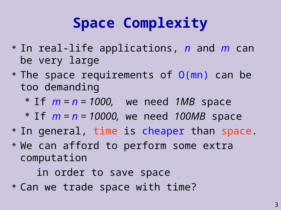
Space Complexity

In real-life applications, n and m can be very large The space requirements of O(mn) can be too

demanding If m = n = 1000, we need 1MB space If m = n = 10000, we need 100MB space

In general, time is cheaper than space. We can afford to perform some extra computation

in order to save space Can we trade space with time?

4

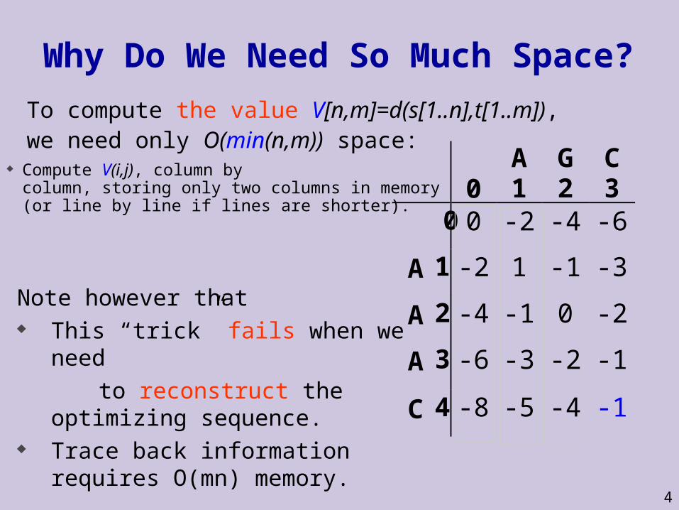
Why Do We Need So Much Space?

Compute V(i,j), column by column, storing only two columns in memory (or line by line if lines are shorter). 0

-2

-4

-6

-8

-2

1

-1

-3

-5

-4

-1

0

-2

-4

-6

-3

-2

-1

-1

0A1

G2

C3

0

A 1

A 2

A 3

C 4

Note however that This “trick” fails when we need

to reconstruct the optimizing sequence.

Trace back information requires O(mn) memory.

To compute the value V[n,m]=d(s[1..n],t[1..m]), we need only O(min(n,m)) space:

5

Hirshberg’s Space Efficient Algorithm

If n=1, align s[1,1] and t[1,m] Else, find position (n/2, j) at which an optimal

alignment crosses the midline s

t

Construct alignments A=s[1,n/2] vs t[1,j] B=s[n/2+1,n] vs

t[j+1,m] Return AB

Input: Sequences s[1,n] and t[1,m] to be aligned.

Idea: Divide and conquer

6

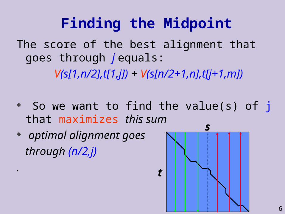
Finding the Midpoint

The score of the best alignment that goes through j equals:

V(s[1,n/2],t[1,j]) + V(s[n/2+1,n],t[j+1,m])

So we want to find the value(s) of j that maximizes this sum

optimal alignment goes through (n/2,j).

s

t

7

Finding the MidpointThe score of the best alignment that goes through j

equals:V(s[1,n/2],t[1,j]) + V(s[n/2+1,n],t[j+1,m])

Want to compute these two quantities for all values of j. Let F[i,j] = V(s[1,i],t[1,j]) (“forward”). Compute F[i,j] just like we did before. Get all F[n/2,j]

s

t

8

Finding the Midpoint

The score of the best alignment that goes through j equals:

V(s[1,n/2],t[1,j]) + V(s[n/2+1,n],t[j+1,m])

We want to compute these two quantities

for all values of j. Let B[i,j] = V(s[i+1,n],t[j+1,m]) (“backwars”) Hey - B[i,j] is not something we already saw.

s

t

9

Finding the Midpoint

B[i,j] = V(s[i+1,n],t[j+1,m]) is the value of optimal alignment between a suffix of s and a suffix of t.

But in the lecture we only talked about alignments between two prefixes.

Don’t be ridiculous: Think backwards. B[i,j] is the value of optimal alignment between prefixes of s reversed and t reversed.

s

t

10

Algorithm: Finding the Midpoint

Define F[i,j] = V(s[1,i],t[1,j]) (“forward”) B[i,j] = V(s[i+1,n],t[j+1,m]) (“backward”)

F[i,j] + B[i,j] = score of best alignment through (i,j)

We compute F[i,j] as we did before We compute B[i,j] in exactly the same manner,

going “backward” from B[n,m]

11

Space Complexity of AlgorithmWe first find j where F[i,n/2] + B[n/2+1,j] ismaximized. To do this, we need just to compute values of F[,],B[,], which take O(n+m) space.

Once midpoint computed, we keep it in memory, (consant memory), then solve recursive the sub-problems.Recursion depth is O(log n). Memory requirement

isO(1) per level + O(m+n) reusable memory at all recursion levels = O(n+m) memory overall.

12

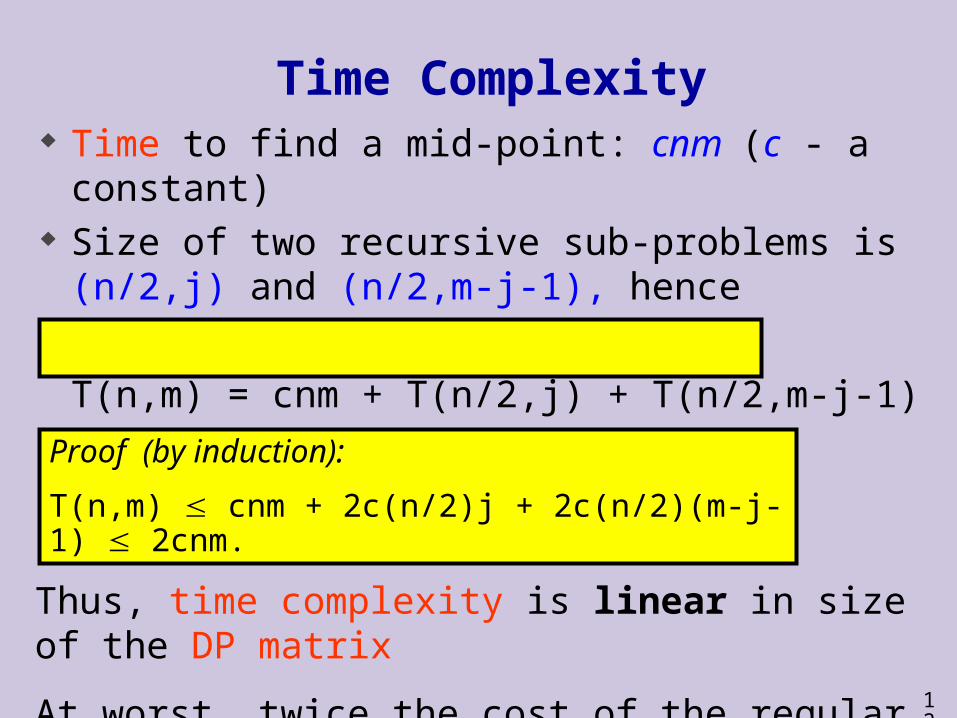
Time Complexity Time to find a mid-point: cnm (c - a constant) Size of two recursive sub-problems is

(n/2,j) and (n/2,m-j-1), hence

T(n,m) = cnm + T(n/2,j) + T(n/2,m-j-1)

Lemma: T(n,m) 2cnmProof (by induction):

T(n,m) cnm + 2c(n/2)j + 2c(n/2)(m-j-1) 2cnm.

Thus, time complexity is linear in size of the DP matrix

At worst, twice the cost of the regular solution.

13

Local Alignment

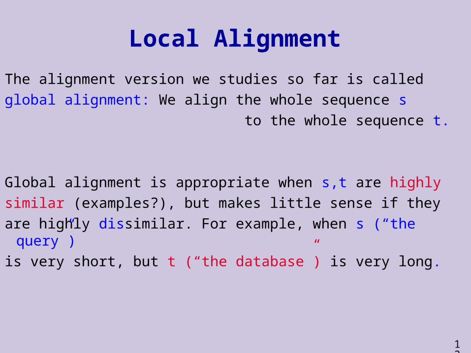
The alignment version we studies so far is called

global alignment: We align the whole sequence s

to the whole sequence t.

Global alignment is appropriate when s,t are highly

similar (examples?), but makes little sense if they

are highly dissimilar. For example, when s (“the query”)

is very short, but t (“the database”) is very long.

14

Local Alignment

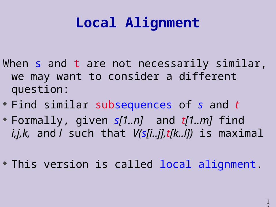
When s and t are not necessarily similar, we may want to consider a different question:

Find similar subsequences of s and t Formally, given s[1..n] and t[1..m] find i,j,k, and l

such that V(s[i..j],t[k..l]) is maximal

This version is called local alignment.

15

Local Alignment

As before, we use dynamic programming We now want to setV[i,j] to record the maximum

value over all alignments of a suffix of s[1..i] and a suffix of t[1..j] In other words, we look for a suffix of a prefix. How should we change the recurrence rule? Same as before but with an option to start afresh

The result is called the Smith-Waterman algorithm, after its inventors (1981).

16

Local Alignment

New option: We can start a new alignment instead of extending

a previous one

V[i, j] (s[i 1], t[ j 1])

V[i 1, j 1] max V[i, j 1] (s[i 1], )

V[i 1, j] ( , t[ j 1])

0

Alignment of empty suffixesV[0,0] 0

V[i 1,0] max( , V[i,0] (s[i 1], ))

V[0, j 1] max( , V[0, j] ( , t[ j 1 )0 ]

0

)

17

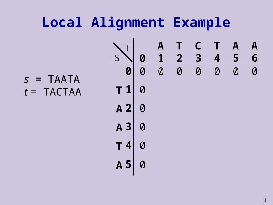
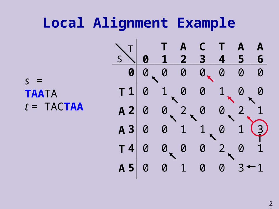
Local Alignment Example

0

A 1

T 2

C 3

T 4

A 5

A 6

0 0 0 0 0 0 0 0

T 1 0

A 2 0

A 3 0

T 4 0

A 5 0

s = TAATAt = TACTAA

ST

18

Local Alignment Example

0

T 1

A 2

C 3

T 4

A 5

A 6

0 0 0 0 0 0 0 0

T 1 0 1 0 0 1 0 0

A 2 0 0 2 0 0 2 1

A 3 0

T 4 0

A 5 0

s = TAATAt = TACTAA

ST

19

Local Alignment Example

0T1

A2

C3

T4

A5

A6

0 0 0 0 0 0 0 0

T 1 0 1 0 0 1 0 0

A 2 0 0 2 0 0 2 1

A 3 0 0 1 1 0 1 3

T 4 0 0 0 0 2 0 1

A 5 0 0 1 0 0 3 1

s = TAATAt = TACTAA

ST

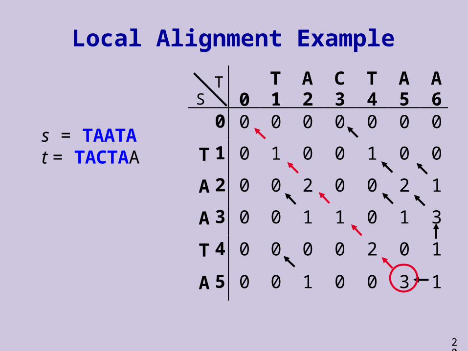
20

Local Alignment Example

0T1

A2

C3

T4

A5

A6

0 0 0 0 0 0 0 0

T 1 0 1 0 0 1 0 0

A 2 0 0 2 0 0 2 1

A 3 0 0 1 1 0 1 3

T 4 0 0 0 0 2 0 1

A 5 0 0 1 0 0 3 1

s = TAATAt = TACTAA

ST

21

Local Alignment Example

0T1

A2

C3

T4

A5

A6

0 0 0 0 0 0 0 0

T 1 0 1 0 0 1 0 0

A 2 0 0 2 0 0 2 1

A 3 0 0 1 1 0 1 3

T 4 0 0 0 0 2 0 1

A 5 0 0 1 0 0 3 1

s = TAATAt = TACTAA

ST

22

Two related notions for sequences comparisons:Roughly• Similarity of 2 sequences? Count matches.• Distance of 2 sequences? Count mismatches.

Similarity can be either positive or negative.Distance is always non-negative (>0). Identical sequences have zero (0) distance.

HIGH SIMILARITY = LOW DISTANCE

Similarity vs. Distance

23

Similarity vs. Distance

So far, the scores of alignments we dealt with weresimilarity scores.

We sometimes want to measure distance between sequencesrather than similarity (e.g. in evolutionary reconstruction).

Can we convert one score to the other (similarity to distance)?

What should a distance function satisfy?

Of the global and local versions of alignment, only one is appropriate for distance formulation.

24

Remark: Edit DistanceIn many stringology applications, one often talks about the edit

distance between two sequences, defined to be the minimum

number of edit operations needed to transform one sequence

into the other. “no change” is charged 0 “replace” and “indel” are charged 1

This problem can be solved as a global distance alignment

problem, using DP. It can easily be generalized to have unequal

“costs” of replace and indel.

To satisfy triangle inequality, “replace” should not be

more expensive than two “indels”.

25

Alignment with affine gap scores

Observation: Insertions and deletions often occur in blocks longer than a single nucleotide.

mlengthofgapPmlengthofgapP )1()(

Consequence: Standard scoring of alignment studied in lecture, which give a constant penalty d per gap unit , does not score well this phenomenon; Hence, a better gap score model is needed.

Question: Can you think of an appropriate change to the scoring system for gaps?

26

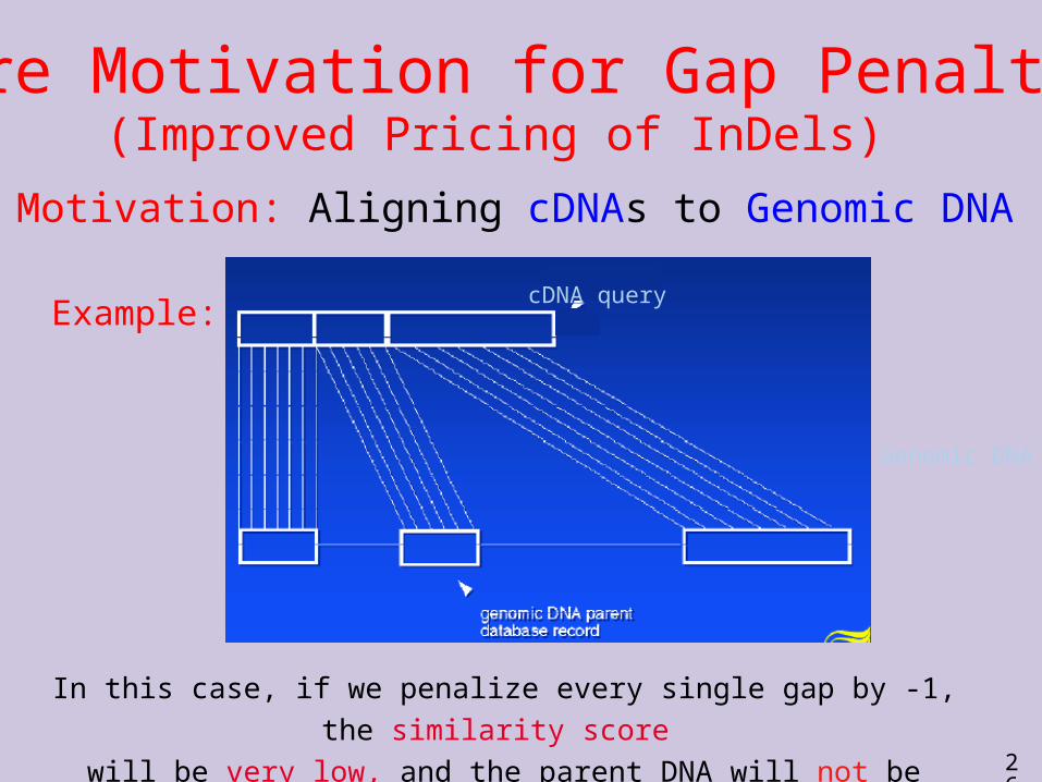
(Improved Pricing of InDels)

Motivation: Aligning cDNAs to Genomic DNA

Example:

In this case, if we penalize every single gap by -1, the similarity score

will be very low, and the parent DNA will not be picked up.

Genomic DNA

cDNA query

More Motivation for Gap Penalties

27

Variants of Sequence Alignment

We have seen two variants of sequence alignment : Global alignment Local alignment

Other variants, in the books and in recitation, can also be solved with the same basic idea of dynamic programming.

:

1. Using an affine cost V(g) = -d –(g-1)e for gaps of length g. The –d (“gap open”) is for introducing a gap, and the –e (“gap extend”) is for continuing the gap. We used d=e=2 in the naïve scoring, but could use smaller e.

2. Finding best overlap

28

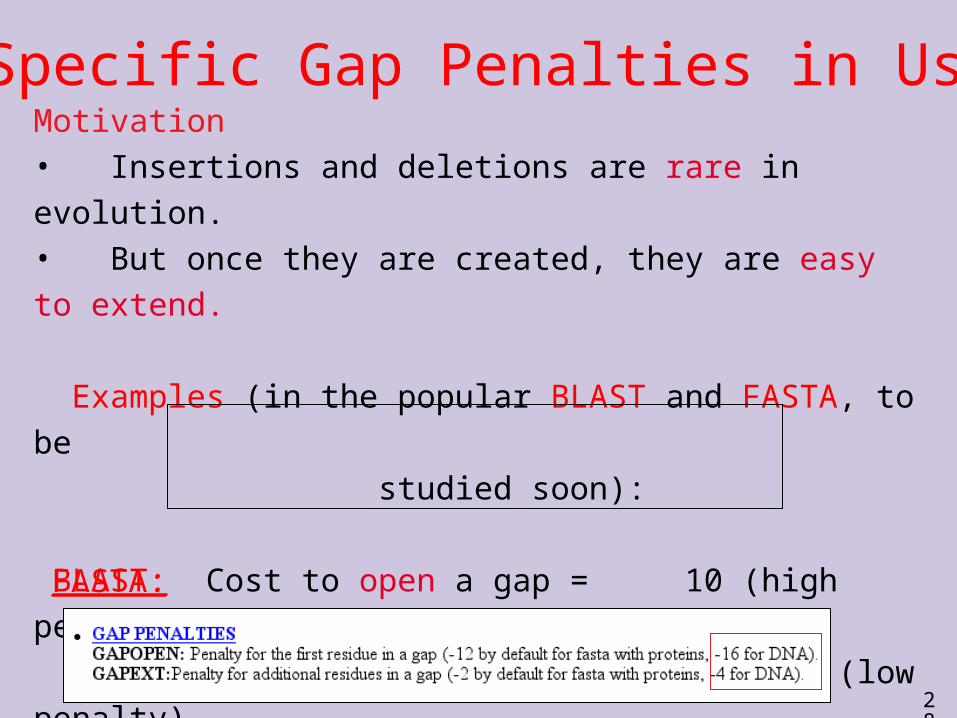
Motivation• Insertions and deletions are rare in evolution. • But once they are created, they are easy to extend.

Examples (in the popular BLAST and FASTA, to be studied soon):

BLAST: Cost to open a gap = 10 (high penalty). Cost to extend a gap = 0.5 (low penalty).

FASTA:

Specific Gap Penalties in Use

29

Alignment in Real Life One of the major uses of alignments is to find

sequences in a large “database” (e.g. genebank). The current protein database contains about 100

millions (i.e.,108) residues! So searching a 1000 long target sequence requires to evaluate about 1011 matrix cells which will take approximately three hours for a processor running 10 millions evaluations per second.

Quite annoying when, say, 1000 target sequences need to be searched because it will take about four months to run.

So even O(nm) is too slow. In other words, forget it!

30

Heuristic Fast Search

Instead, most searches rely on heuristic procedures These are not guaranteed to find the best match Sometimes, they will completely miss a high-scoring

match

We now describe the main ideas used by the best known of these heuristic procedures.

31

Basic Intuition

Almost all heuristic search procedures are based on the observation that good real-life alignments often contain long runs with no gaps (mostly

matches, maybe a few mismatches).

These heuristic try to find significant gap-less runs and then extend them.

32

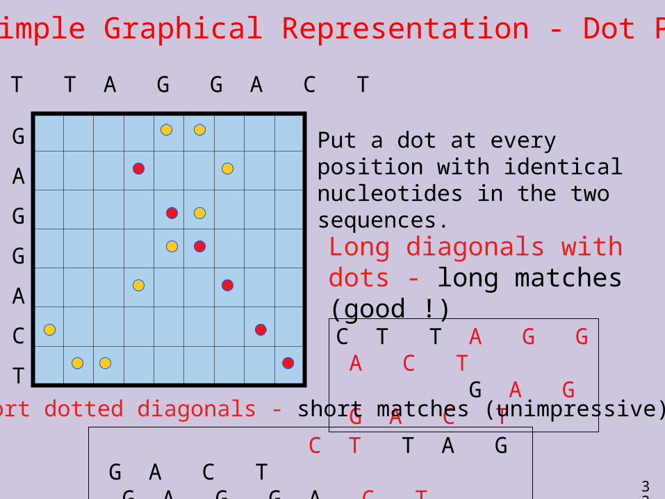
A Simple Graphical Representation - Dot Plot

Put a dot at every position with identical nucleotides in the two sequences.

C T T A G G A C T

G

A

G

G

A

C

T

Sequences:

C T T A G G A C TG A G G A C T

33

A Simple Graphical Representation - Dot Plot

Put a dot at every position with identical nucleotides in the two sequences.

C T T A G G A C T

G

A

G

G

A

C

T

Long diagonals with dots - long matches (good !)C T T A G G A C T G A G G A C T

Short dotted diagonals - short matches (unimpressive)

C T T A G G A C T G A G G A C T

34

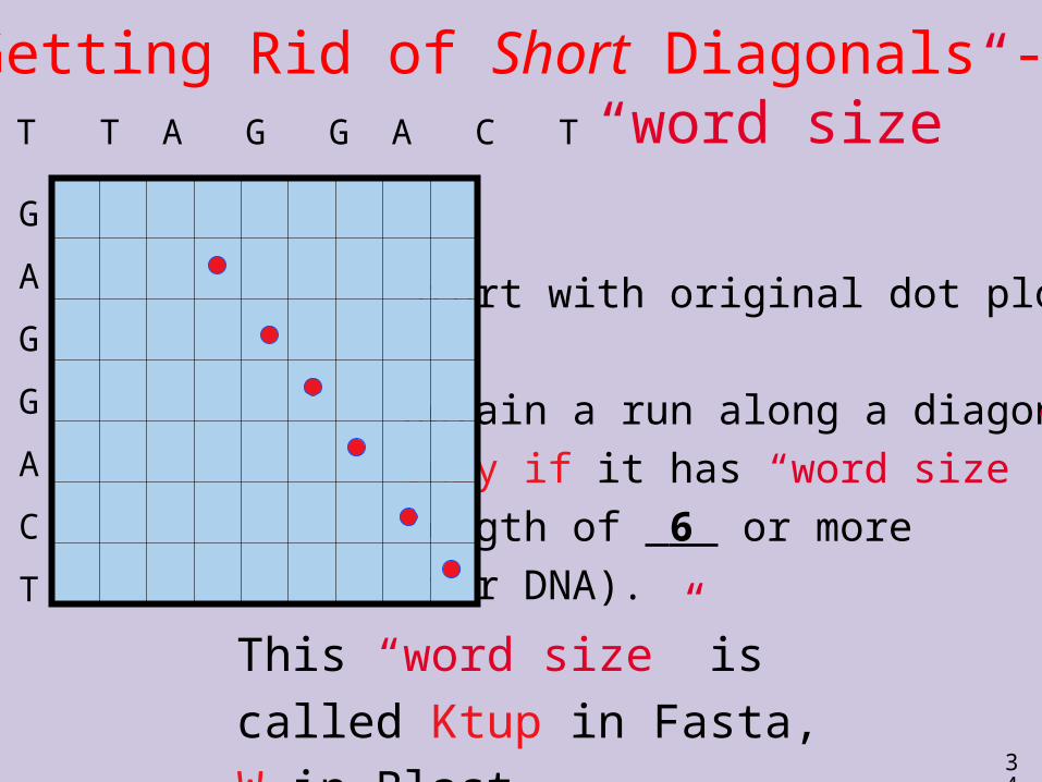
Getting Rid of Short Diagonals - “word size”

Start with original dot plot.

Retain a run along a diagonalonly if it has “word size”

length of 6 or more (for DNA).

This “word size” is called Ktup in Fasta, W in Blast

C T T A G G A C T

G

A

G

G

A

C

T

35

Banded DP

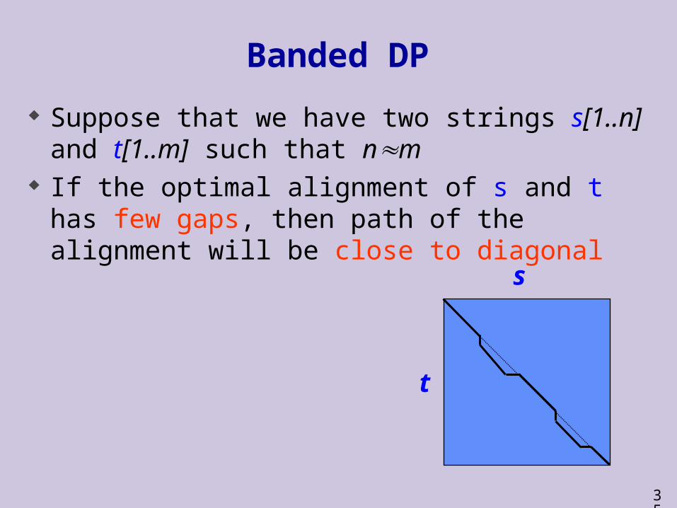
Suppose that we have two strings s[1..n] and t[1..m] such that nm

If the optimal alignment of s and t has few gaps, then path of the alignment will be close to diagonal

s

t

36

Banded DP To find such a path, it suffices to search in a

diagonal region of the matrix. If the diagonal band has width k, then the dynamic

programming step takes O(kn). Much faster than O(n2) of standard DP. Boundary values set to 0 (local alignment)

s

t kV[i+1, i+k/2 +1]Out of range

V[i, i+k/2+1]V[i,i+k/2]

Note that for diagonals i-j = constant.

37

Banded DP for local alignment

Problem: Where is the banded diagonal ? It need not be the main diagonal when looking for a good local alignment.

How do we select which subsequences to align using banded DP?

s

tk

We heuristically find potential diagonals and evaluate them using Banded DP.

This is the main idea of FASTA.

38

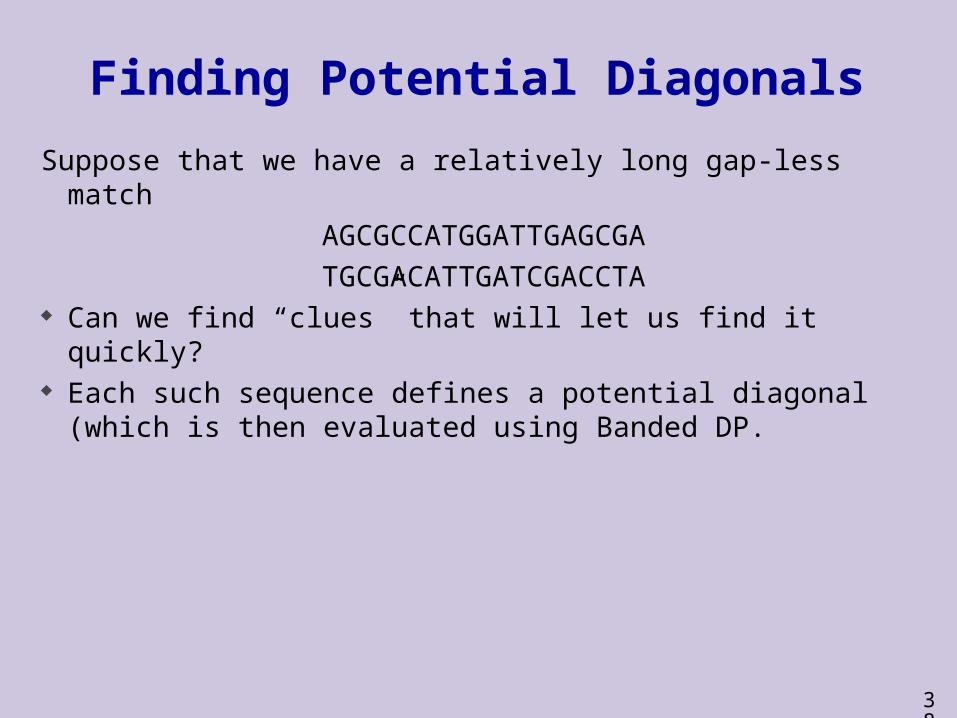
Finding Potential Diagonals

Suppose that we have a relatively long gap-less match

AGCGCCATGGATTGAGCGA

TGCGACATTGATCGACCTA Can we find “clues” that will let us find it quickly? Each such sequence defines a potential diagonal (which is

then evaluated using Banded DP.

39

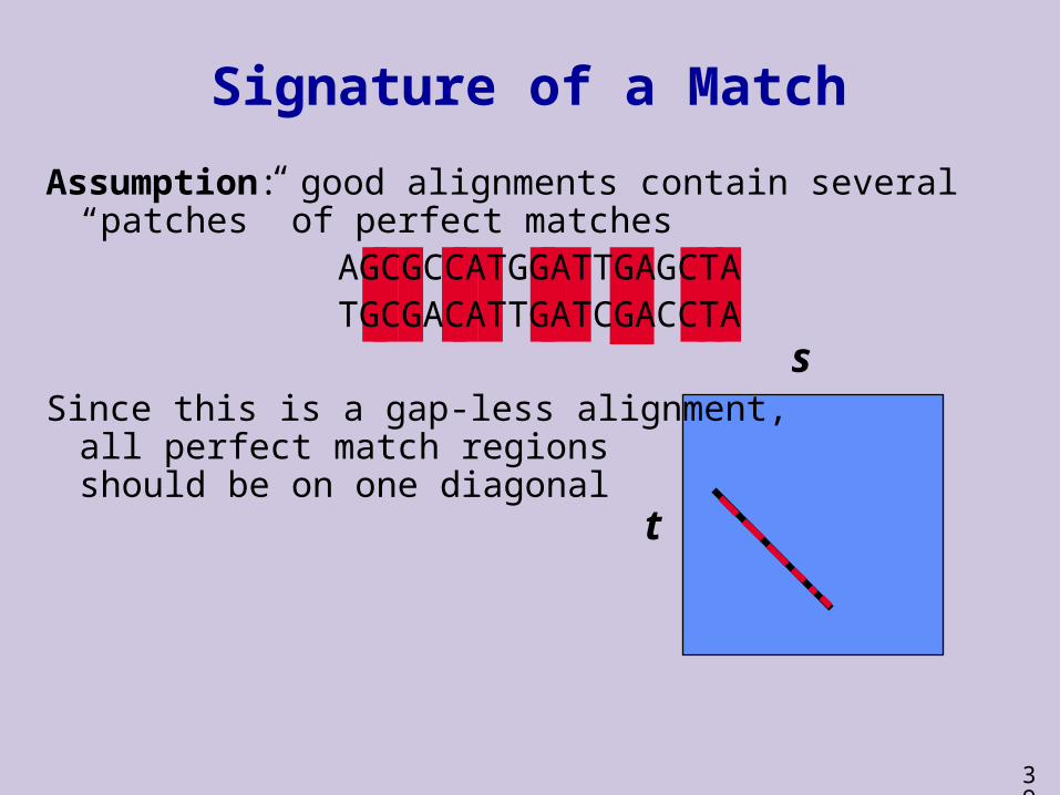
Signature of a Match

s

t

Assumption: good alignments contain several “patches” of perfect matches

AGCGCCATGGATTGAGCTATGCGACATTGATCGACCTA

Since this is a gap-less alignment, all perfect match regionsshould be on one diagonal

40

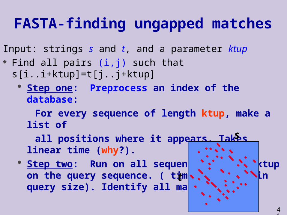
FASTA-finding ungapped matches

Input: strings s and t, and a parameter ktup Find all pairs (i,j) such that s[i..i+ktup]=t[j..j+ktup] Locate sets of matching pairs that are on the same diagonal By sorting according to the difference i-j

Compute the score for the diagonal that contains all these pairs

s

t

41

FASTA-finding ungapped matches

Input: strings s and t, and a parameter ktup Find all pairs (i,j) such that s[i..i+ktup]=t[j..j+ktup] Step one: Preprocess an index of the database:

For every sequence of length ktup, make a list of

all positions where it appears. Takes linear time (why?). Step two: Run on all sequences of size ktup on the

query sequence. ( time is linear in query size). Identify all matches (i,j).

s

t

42

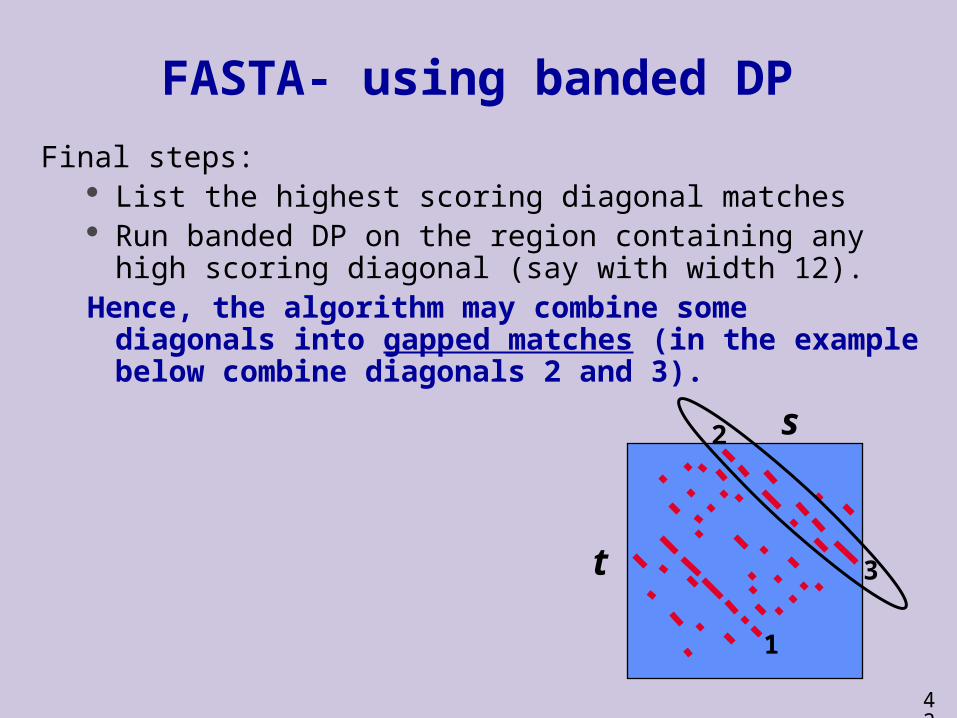
FASTA- using banded DP

Final steps: List the highest scoring diagonal matches Run banded DP on the region containing any high scoring

diagonal (say with width 12).Hence, the algorithm may combine some diagonals into

gapped matches (in the example below combine diagonals 2 and 3).

s

t 3

2

1

43

FASTA- practical choices

Some implementation choices / tricks have not been explicated herein.

s

t

Most applications of FASTA use fairly small ktup (2 for proteins, and 6 for DNA).

Higher values are faster, yielding fewer diagonals to search around, but increase the chance to miss the optimal local alignment.

44

Effect of Word Size (ktup)

Large word size - fast, less sensitive, more selective:distant relatives do not have many runs of matches,un-related sequences stand no chance to be selected.Small word size - slow, more sensitive, less selective.

Example: If ktup = 3, we will consider all substrings containing TCG in this sequence (very sensitive compared to large word size, but less selective. Will find all TCGs).

45

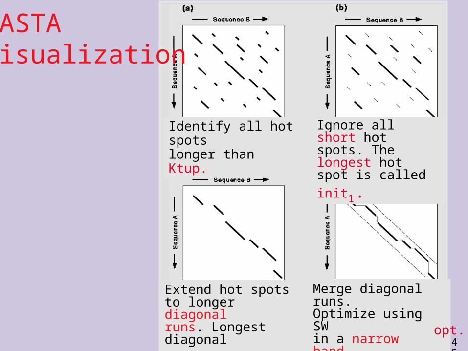
FASTAVisualization

Identify all hot spots longer than Ktup.

Ignore all short hot spots. The longest hot spot is called init1.

Extend hot spots to longer diagonal runs. Longest diagonal

run is initn.

Merge diagonal runs. Optimize using SW in a narrow band. Best result is called

opt.

46

FastA OutputFastA produces a list, where each entry looks like:

EM_HUM:AF267177 Homo sapiens glucocer (5420) [f] 3236 623 1.1e-176

The database name and entry (accession

numbers).

Then comes the species.

and a short gene name.

The length of the sequence.

Scores:

Similarity score of the optimal alignment (opt).

The bits score,

and the E-value.

Both measure the statistical significance of the alignment.

47

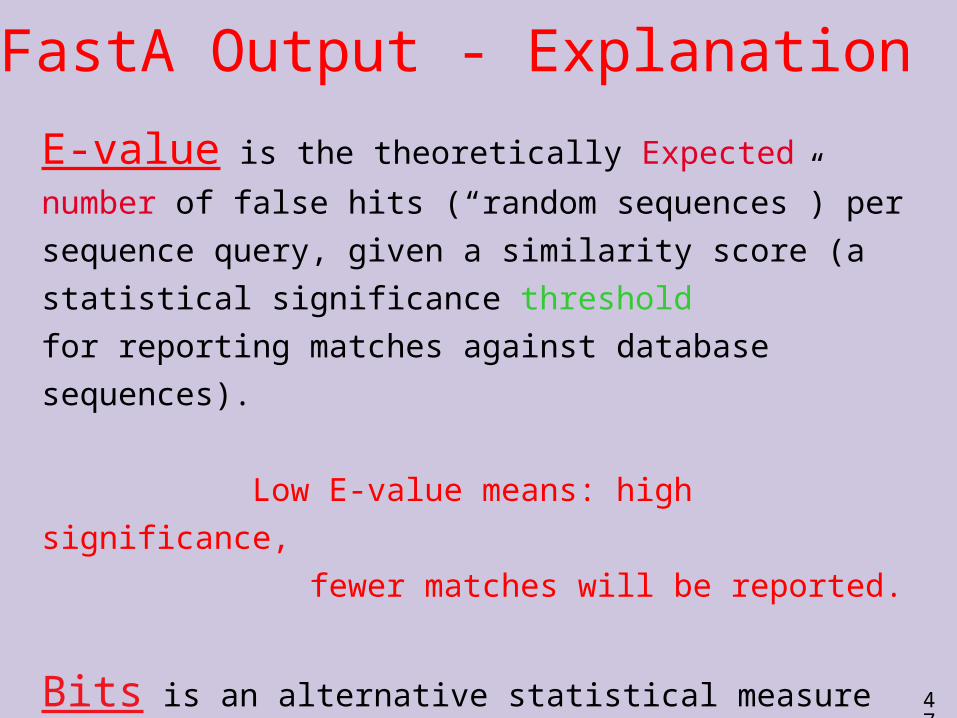
FastA Output - Explanation

E-value is the theoretically Expected number of

false hits (“random sequences”) per sequence query,

given a similarity score (a statistical significance

threshold

for reporting matches against database sequences).

Low E-value means: high significance,

fewer matches will be reported.

Bits is an alternative statistical measure for

significance.

High bits means high significance. Some versions also

display z-score, a measure similar to Bits.

48

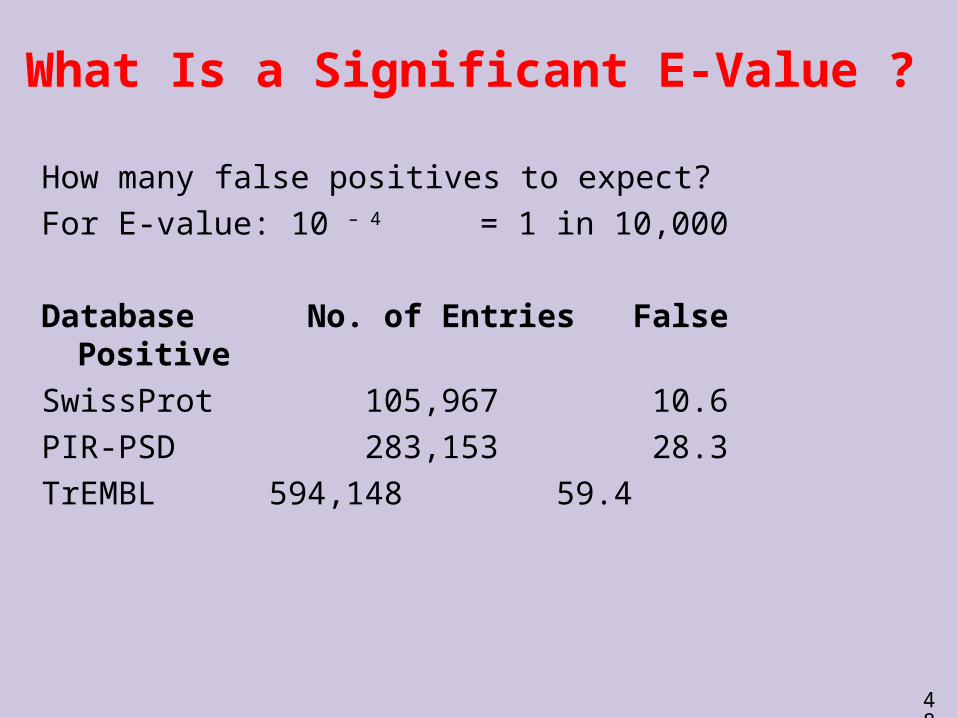
What Is a Significant E-Value ?

How many false positives to expect? For E-value: 10 – 4 = 1 in 10,000

Database No. of Entries False PositiveSwissProt 105,967 10.6PIR-PSD 283,153 28.3TrEMBL 594,148 59.4

49

Expect Value (E) and Score (S) The probability that an alignment score as good as the one found between a query sequence and a database sequence would be found by random chance.

Example: Score E-value108 10 –2

= >1 in 100 will have the same score.

For a given score, the E-value increases with increasing size of the database. For a given database, the E-value decreases exponentially with

increasing score.

50

opt

the “usual” bell curve

“Unexpected”, high score sequences (signal vs noise)

A Histogram forobserved (=) vs expected (*)

51

FASTA-summary

Input: strings s and t, and a parameter ktup = 2 or 6 or user’s choice, depending on the application.

Output: A high score local alignment

1. Find pairs of matching substrings s[i..i+ktup]=t[j..j+ktup]

2. Extend to ungapped diagonals3. Extend to gapped alignment using banded DP

4. Can you think of example for pairs of sequences that have high local similarity scores but will be missed by FASTA ?

52

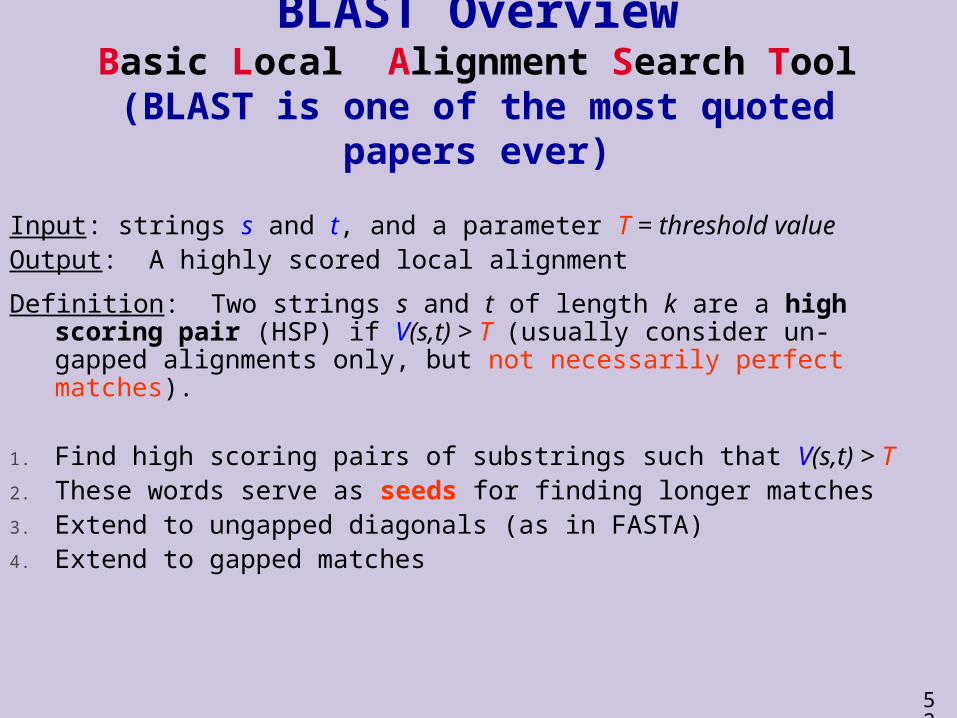
BLAST OverviewBasic Local Alignment Search Tool

(BLAST is one of the most quoted papers ever)

Input: strings s and t, and a parameter T = threshold valueOutput: A highly scored local alignment

Definition: Two strings s and t of length k are a high scoring pair (HSP) if V(s,t) > T (usually consider un-gapped alignments only, but not necessarily perfect matches).

1. Find high scoring pairs of substrings such that V(s,t) > T2. These words serve as seeds for finding longer matches3. Extend to ungapped diagonals (as in FASTA)4. Extend to gapped matches

53

BLAST Overview (cont.)

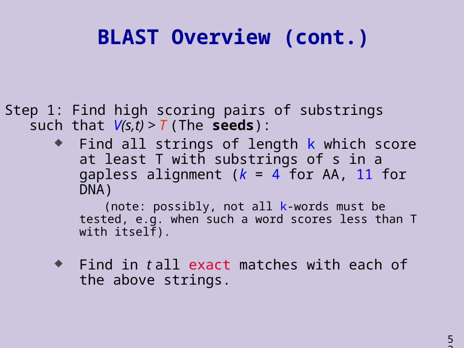
Step 1: Find high scoring pairs of substrings such that V(s,t) > T (The seeds):

Find all strings of length k which score at least T with substrings of s in a gapless alignment (k = 4 for AA, 11 for DNA)

(note: possibly, not all k-words must be tested, e.g. when such a word scores less than T with itself).

Find in t all exact matches with each of the above strings.

54

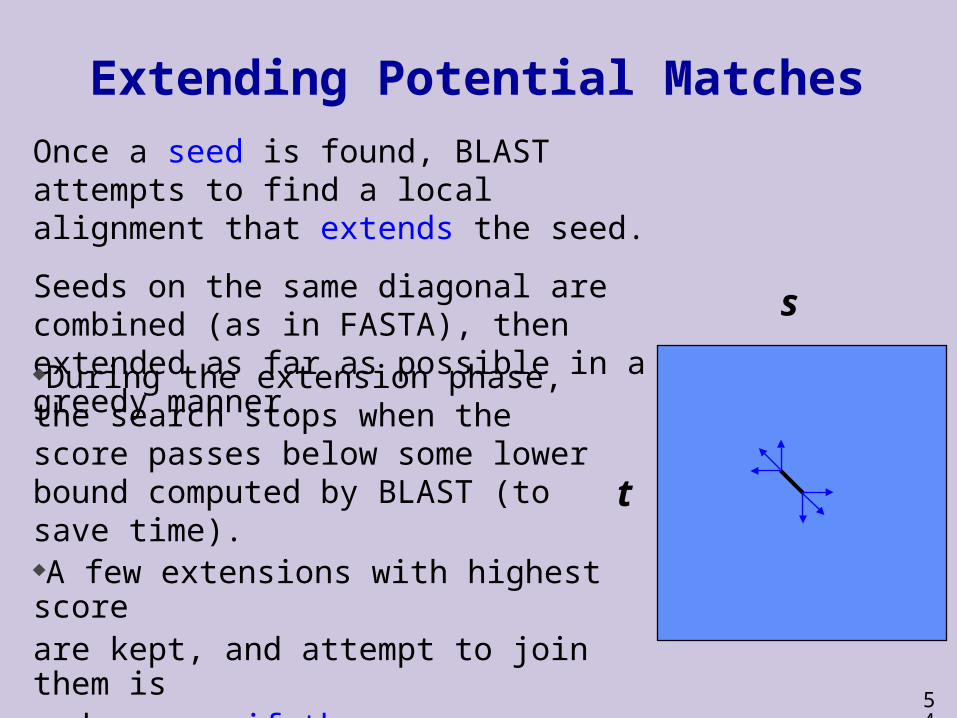
Extending Potential Matches

s

t

Once a seed is found, BLAST attempts to find a local alignment that extends the seed.

Seeds on the same diagonal are combined (as in FASTA), then extended as far as possible in a greedy manner.

During the extension phase, the search stops when the score passes below some lower bound computed by BLAST (to save time).A few extensions with highest score are kept, and attempt to join them is made, even if they are on distant diagonals, provided the join improves both scores.

55

BLAST Facts

BLAST is the most frequently used sequence alignment program.

An impressive statistical theory, employing issues of the renewal

theorem, random walks, and sequential analysis was developed

for analyzing the statistical significance of BLAST results. These

are all out of scope for this course.

See the book ``Statistical Methods in BioInformatics” by

Ewens and Grant (Springer 2001) for more details.

56

Scoring Functions, Reminder

So far, we discussed dynamic programming algorithms for global alignment local alignment

All of these assumed a scoring function:

that determines the value of perfect matches, substitutions, insertions, and deletions.

}){(}){(:

57

Where does the scoring function come from ?

We have defined an additive scoring function by specifying a function ( , ) such that (x,y) is the score of replacing x by y (x,-) is the score of deleting x (-,x) is the score of inserting x

But how do we come up with the “correct” score ?

Answer: By encoding experience of what are similar sequences for the task at hand. Similarity depends on time, evolution trends, and sequence types.

58

Why probability setting is appropriate to define and interpret a scoring function ?

• Similarity is probabilistic in nature because biological changes like mutation, recombination, and selection, are random events.

• We could answer questions such as:• How probable it is for two sequences to be similar?• Is the similarity found significant or spurious?• How to change a similarity score when, say, mutation rate of a specific area on the chromosome becomes known ?

59

A Probabilistic Model

For starters, will focus on alignment without indels. For now, we assume each position (nucleotide /amino-

acid) is independent of other positions. We consider two options:

M: the sequences are Matched (related)

R: the sequences are Random (unrelated)

60

Unrelated Sequences

Our random model R of unrelated sequences is simple Each position is sampled independently from a

distribution over the alphabet We assume there is a distribution q() that

describes the probability of letters in such positions.

Then:

i

R(s[1..n], t[1..n] | ) q q(s[i]) (P t[i])

61

Related Sequences

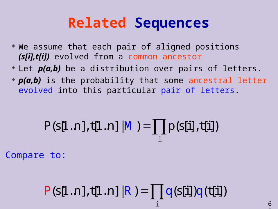
We assume that each pair of aligned positions (s[i],t[i]) evolved from a common ancestor

Let p(a,b) be a distribution over pairs of letters. p(a,b) is the probability that some ancestral letter

evolved into this particular pair of letters.

i

i

P(s[1..n], t[1..n] | ) p(s[i], t[i])

(

M

Rs[1..n], t[1..n] | ) (s[i]) (t[iP )q ]q

Compare to:

62

Odd-Ratio Test for Alignment

i

ii

p(s[i], t[i])P(s, t | ) p(s[i], t[i])

QP(s, t | ) q(s[i])q(t[i]) q(s[i])q(t[R i])

M

If Q > 1, then the two strings s and t are more likely tobe related (M) than unrelated (R).

If Q < 1, then the two strings s and t are more likely tobe unrelated (R) than related (M).

63

Score(s[i],t[i])

Log Odd-Ratio Test for AlignmentTaking logarithm of Q yields

])[(])[(

])[],[(log

])[(])[(

])[],[(log

)|,(

)|,(log

itqisq

itisp

itqisq

itisp

RtsP

MtsP

ii

If log Q > 0, then s and t are more likely to be related.If log Q < 0, then they are more likely to be unrelated.

How can we relate this quantity to a score function ?

64

Probabilistic Interpretation of Scores

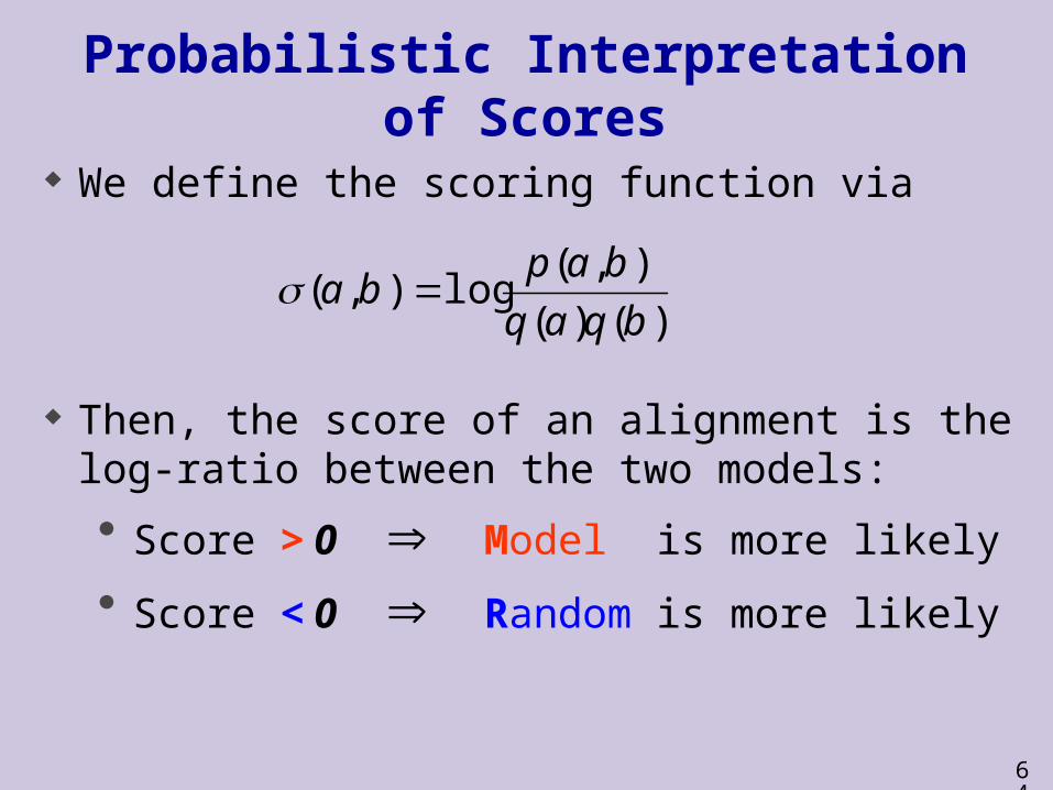
We define the scoring function via

Then, the score of an alignment is the log-ratio between the two models:

Score > 0 Model is more likely

Score < 0 Random is more likely

)()(),(

log),(bqaq

bapba

65

Modeling Assumptions

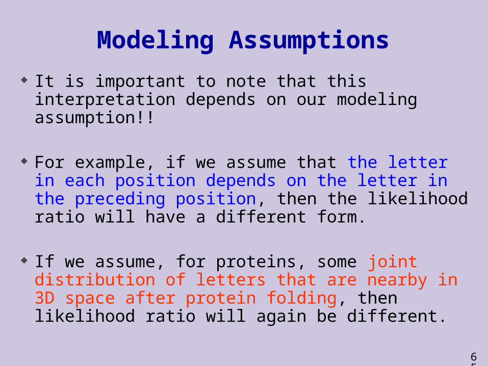
It is important to note that this interpretation depends on our modeling assumption!!

For example, if we assume that the letter in each position depends on the letter in the preceding position, then the likelihood ratio will have a different form.

If we assume, for proteins, some joint distribution of letters that are nearby in 3D space after protein folding, then likelihood ratio will again be different.

66

Estimating Probabilities

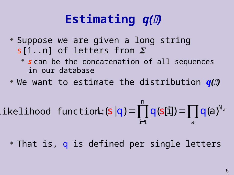
Suppose we are given a long string s[1..n] of letters from

We want to estimate the distribution q(·) that generated the sequence

How should we go about this?

We build on the theory of parameter estimation in statistics using either maximum likelihood estimation or the Bayesian approach .

67

Estimating q()

Suppose we are given a long string s[1..n] of letters from s can be the concatenation of all sequences in our

database We want to estimate the distribution q()

That is, q is defined per single letters

a

nN

i 1 a

qL( | q) ( [is s ]) )q(a

Likelihood function:

68

Estimating q() (cont.)

How do we define q?

aq(a)N

n

a

nN

i 1 a

L(s | q) q(s[i]) q(a)

Likelihood function:

ML parameters

(Maximum Likelihood)

69

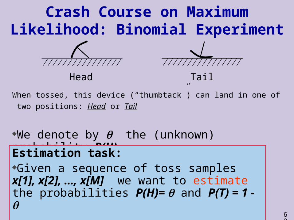
Crash Course on Maximum Likelihood: Binomial Experiment

When tossed, this device (“thumbtack”) can land in one of

two positions: Head or Tail

Head Tail

We denote by the (unknown) probability P(H).

Estimation task:Given a sequence of toss samples x[1], x[2], …, x[M] we want to estimate the probabilities P(H)= and P(T) = 1 -

70

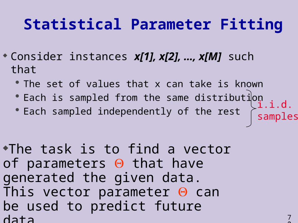
Statistical Parameter Fitting

Consider instances x[1], x[2], …, x[M] such that The set of values that x can take is known Each is sampled from the same distribution Each sampled independently of the rest

i.i.d.samples

The task is to find a vector of parameters that have generated the given data. This vector parameter can be used to predict future data.

71

The Likelihood Function How good is a particular ?

It depends on how likely it is to generate the observed data

The likelihood for the sequence H,T, T, H, H is

m

D mxPDPL )|][()|()(

)1()1()(DL

0 0.2 0.4 0.6 0.8 1

L()

72

Sufficient Statistics

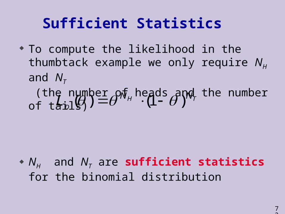
To compute the likelihood in the thumbtack example we only require NH and NT

(the number of heads and the number of tails)

NH and NT are sufficient statistics for the binomial distribution

THD

NNL )1()(

73

Sufficient Statistics

A sufficient statistic is a function of the data that summarizes the relevant information for the likelihood

Datasets

Statistics

Formally, s(D) is a sufficient statistics if for any two datasets D and D’

s(D) = s(D’ ) LD() = LD’ ()

74

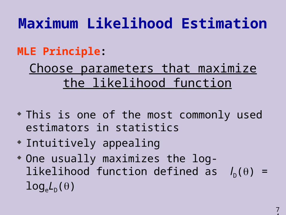
Maximum Likelihood Estimation

MLE Principle:

Choose parameters that maximize the likelihood function

This is one of the most commonly used estimators in statistics

Intuitively appealing One usually maximizes the log-likelihood

function defined as lD() = logeLD()

75

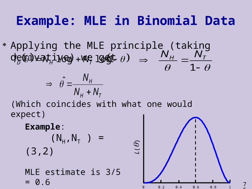
Example: MLE in Binomial Data

Applying the MLE principle (taking derivative) we get 1loglog THD NNl

1TH NN

0 0.2 0.4 0.6 0.8 1

L()

Example:(NH,NT ) = (3,2)

MLE estimate is 3/5 = 0.6

TH

H

NN

N

(Which coincides with what one would expect)

77

Estimating p(·,·)

Intuition: Find pair of aligned sequences s[1..n], t[1..n], Estimate probability of pairs:

The sequences s and t can be the concatenation of many aligned pairs from the database

n

Nbap ba,),(

Number of times a is

aligned with b in (s,t)

78

Problems in Estimating p(·,·)

How do we find pairs of aligned sequences? How far is the ancestor ? earlier divergence low sequence similarity recent divergence high sequence similarity

Does one letter mutate to the other or are they both mutations of a common ancestor having yet another residue/nucleotide acid ?

79

Estimating p(·,·) for proteins

An accepted mutation is a mutation due to an alignment of closely related protein sequences. For example, Hemoglobin alpha chain in humans and other organisms (homologous proteins).

80

Estimating p(·,·) for proteins

aNq(a)

n

abf

aaf f

Generate a large diverse collection of accepted mutations.

Recall that

Define: to be the number of mutations a b,

to be the total number of mutations of a,

and to be the total number of amino acids involvedin a mutation.

Note that f is twice the number of mutations.

a abb| b af f

81

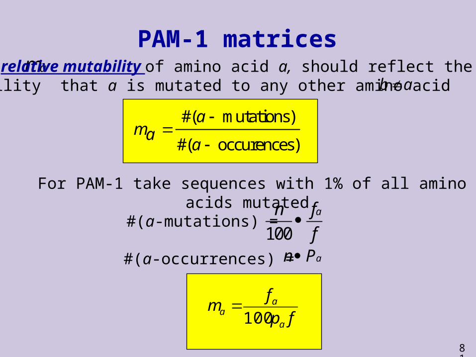
#( mutations)

#( occurences)

ama

a

PAM-1 matrices

fp

fm

a

aa 100

am

For PAM-1 take sequences with 1% of all amino acids mutated.

#(a-mutations) = 100

an f

f

#(a-occurrences) = *aP n

an P

, The relative mutability of amino acid a, should reflect the Probability that a is mutated to any other amino acid :

b a

b a

82

PAM-1 matrices

fp

fm

a

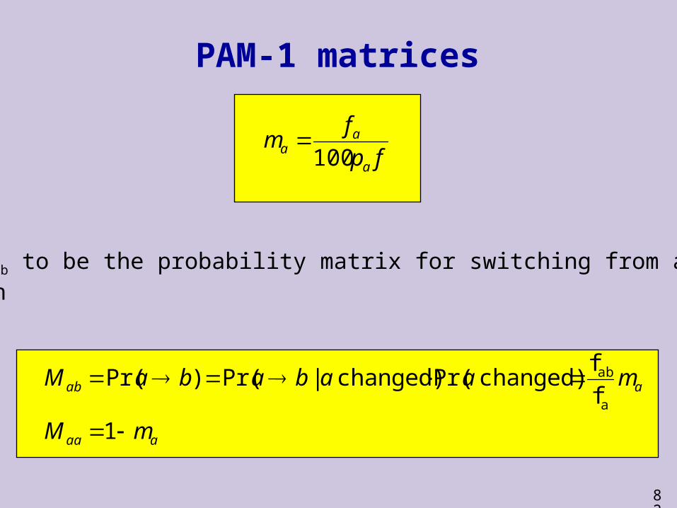
aa 100

Define Mab to be the probability matrix for switching from a to b viaA mutation

aaa

aab

mM

maababaM

1

f

fchanged)Pr(changed)|Pr()Pr(

a

ab

83

Properties of PAM-1 matrices

1b abMNote that

Namely, the probability of not changing and changing sums to 1.

99.0 aaa aMp

Namely, only 1% of amino acids change according to this matrix. Hence the name, 1-Percent Accepted Mutation (PAM).

Also note that

This is a unit of evolutionary change, not time because evolution acts differently on distinct sequence types.

What is the substitution matrix for k units of evolutionary time ?