courses.physics.ucsd.educourses.physics.ucsd.edu/2014/fall/physics215a/allchaps.pdf · chapter 1...
TRANSCRIPT

PHYS 215A: Lectures on Quantum Field Theory
Benjamın GrinsteinUCSD
December 10, 2014

Chapter 1
Introduction
1.1 Why QFT?
As a new student of the subject you may ask Why study Quantum Field Theory(QFT)? Or why do we need QFT? There are many reasons, and I will explain some.
Pair Creation. For starters, particle quantum mechanics (QM) does not accountfor pair creation. In collisions of electrons with sufficiently large energies it isoccasionally observed that out of the collision an electron and a positron are created(in addition to the originating electrons): e−e− → e−e−e+e−. Sufficiently largeenergies means kinetic energies larger than the rest mass of the e−e+ pair, namely2mec
2. Not only does single particle QM not account for this but in this case thecolliding electrons must be relativistic. So we need a relativistic QM that accountsfor particle creation.
But what if we are atomic physicists, and only care about much smaller ener-gies? If we care about high precision, and atomic physicists do, then the fact thatpair creation is possible in principle cannot be ignored. Consider the perturbationtheory calculation of corrections to the n-th energy level, En, of some atomic statein QM:
δEn = 〈n|H ′|n〉+∑k 6=n
〈n|H ′|k〉〈k|H ′|n〉En − Ek
+ · · ·
The second order term involves all states, regardless of their energy. Hence statesinvolving e+e− states give corrections of order
δE
E∼ atomic energy spacing
mec2.
This is, a priori, as important as the relativistic corrections from kinematics,H =
√(mec2)2 + (pc)2 = mec
2 + 12p
2/me − 18p
4/m3ec
2 + · · · . The first relativis-
1
2 CHAPTER 1. INTRODUCTION
tic correction is H ′ = −14(p/mec)
2(p2/2me) so the fractional correction δE/E ∼(p/mec)
2 ∼ (p2/2me)/(mec2), just as in pair creation. We are lucky that for the
Hydrogen atom the pair creation correction happens to be small. But in generalwe have no right to neglect it.
Instability of relativistic QM. Let’s insist in single particle QM and exploresome consequences. Since H =
√(mec2)2 + (pc)2 does not give us a proper dif-
ferential Schrodinger equation, let’s try a wave equation using the square of theenergy, E2 = (mc2)2 + (pc)2, and replacing, as usual, E → i~∂/∂t and ~p→ −i~∇.This leads to the Klein-Gordon wave equation,[
1
c2
∂2
∂t2−∇2 +
µ2
c2
]φ(~x, t) = 0
where µ = mc2/~. Since this is a free particle we look for plane wave solutions,
f+(~x, t) = a+k e−iωkt+i~k·~x and f−(~x, t) = a−k e
iωkt−i~k·~x,
where a± are constants (independent of ~x and t) and
ωk =
√c2~k2 + µ2.
The interpretation of f+ is clear: using E → i~∂/∂t and ~p → −i~∇ we seethat it has energy E = ~ωk and momentum ~p = ~k and these are related byE =
√(mec2)2 + (pc)2. However, we now also have solutions, f− with energy
E = −~ωk (and momentum ~p = −~k). These have negative energy. For the freeparticle this is not a problem since we can start with a particle of some energy,positive or negative, and it will stay at that energy. But as soon as we introduceinteractions, say by making the particle charged and giving it minimal coupling tothe electromagnetic field, the particle can radiate into a lower energy state, butthere is no minimum energy. There is a catastrophic instability.
Dirac proposed an ingenious solution to this catastrophe. Suppose the particleis a fermion, say, an electron. Then start the system from a state in which allthe negative energy states are occupied. We call this the “Dirac sea.” Since notwo fermions can occupy a state with the same quantum numbers, we cannot havean electron with positive energy radiate to become a negative energy state (thatstate is occupied). However, an energetic photon can interact with an electronwith E < −mec
2 and bump it to a state with E > mec2. What results is a state
with a positive energy electron and a hole in the “Dirac sea.” The hole signifiesthe absence of negative energy and negative charge, so it behaves as a particle withpositive energy and positive charge. That is, as the anti-particle of the electron,

1.1. WHY QFT? 3
the positron. So we conclude we cannot have a single particle QM, we are forcedto consider pair creation.
A note in passing: as we will discuss later, relativistic fermions are describedby the Dirac equation. But a solution of the Dirac equation necessarily solvesthe Klein-Gordon equation, so the discussion above is in fact appropriate to thefermionic case.
Klein’s Paradox. There is another way to see the need to include anti-particlesin the solution to the Klein-Gordon equation. As we stated, only if we includeinteractions will we see a problem. But our description of interactions with anelectromagnetic field was heuristic. We can make it more precise by introducinginstead a potential. The simplest case, considered by Klein, is that of a particlein one spatial dimension with a step potential, V (x) = V0 θ(x). Here θ(x) is theHeavyside step-function
θ(x) =
1 x > 0
0 x < 0
and V0 > 0 is a constant with units of energy. We look for solutions with a planewave incident from the left (x < 0 with p = ~k > 0):
ψL(x, t) = e−iωt+ikLx +Re−iωt−ikLx
ψR(x, t) = Te−iωt+ikRx
These solve the Klein-Gordon equation with the shifted energy provided
ckL =√ω2 − µ2 and ckR =
√(ω − ω0)2 − µ2
where ω0 = V0/~. We now determine the transmission (T ) and reflection (T )
coefficients matching the solutions at x = 0; using ψL(t, 0) = ψR(t, 0) and ∂ψL(t,0)∂t =
∂ψR(t,0)∂t we get
T =2kL
kL + kRand R =
kL − kRkL + kR
.
Formally the solution looks just like in the non-relativistic (NR) case. Indeed, forω > µ + ω0 both wave-vectors kL and kR are real, and so are both transmissioncoefficients and we have a transmitted and a reflected wave. Similarly if ω0 − µ <ω < ω0 +µ then kR has a nonzero imaginary part and we have total reflection (thewould be transmitted wave is exponentially damped).
But for V0 > 2mc2, which corresponds to an energy large enough that paircreation is energetically allowed, there is an unusual solution. If µ < ω < ω0 − µ,which means ω − µ > 0 and ω − µ < ω0 − 2µ, we obtain both kL and kR are real,and so are both T and R. There is a non-zero probability that the particle, which

4 CHAPTER 1. INTRODUCTION
has less energy than the height of the barrier (E −mc2 − V0 < 0), is transmitted.This weird situation, called “Klein’s paradox,” can be understood in terms of paircreation. A complete treatment of the problem requires (as far as I know) a fullyquantum field theoretic treatment, so for that we will have to wait until later inthis course. But the result can be easily described: the incident particle is fullyreflected, but is accompanied by particle-antiparticle pairs.
Bohr’s Box. Above we talked about “localizing” a particle. Let’s make this a bitmore precise (not much, though). Suppose that in order to localize a free particlewe put it in a large box. We don;t know where the particle is other than that itis inside the box. If choose the box large enough, of sides Lx,y,z λC , then theuncertainly in its momentum can be small, ∆px,y,z & ~/Lx,y,z. Then the kinetic
energy can be small, E = ~p2
2m ∼~22m(L−2
x + L−2y + L−2
z ). Now suppose one side ofthe box, parallel to the yz plane, is movable (the box is a cylinder, the movablebox is a piston). So we can attempt to localize the particle along the x axis bycompressing it, that is, by decreasing Lx. Once Lx ∼ λC the uncertainty in theenergy of the particle is ∆E ∼ mc2. Now o localize the particle we have introducedinteraction, those of the particle with the walls of the box that keeps it contained.But as we have seen when the energy available exceeds 2mc2 interactions require anon-vanishing probability for pair creation. We conclude that as we try to localizethe particle to within a Compton wavelength, λC = ~/mc, we get instead a statewhich is a combination of the particle plus a particle-antiparticle pair. Or perhapstwo pairs, or three pairs, or . . . . In trying to localize a particle not only we havelost certainty on its energy, as is always the case in QM, but we have also lostcertainty on the number of particles we are trying to localize!
This gives us some physical insight into Klein’s paradox. The potential steplocalizes the particle over distances smaller than a Compton wavelength. Theuncertainty principle then requires that the energy be uncertain by more than theenergy required for pair production. It can be shown that if the step potential isreplaced by a smooth potential that varies slowly between 0 and V0 over distancesd larger than λC then transmission is exponentially damped, but as d is madesmaller than λC Klein’s paradox re-emerges (Sauter).
Democracy. It is well known that elementary particles are indistinguishable:every electron in the world has the same mass, charge and magnetic moment. InNRQM we account for this in an ad-hoc fashion. We write
H =∑i
~p2i
2me+
e
mec~A(~xi) · ~pi + ~B(~xi) · ~µi where ~µi =
ge~2mec
~σi,

1.1. WHY QFT? 5
but we have put in by hand that the mass me, the charge e and the gyromagneticratio g are the same for all electrons. Where does this democratic choice comefrom?
Moreover, photons, which are quanta of the electromagnetic field, are intro-duced by second quantizing the field. But electrons are treated differently. Un-democratic! If instead we insist that all particles are quanta of field excitations notonly we will have a more democratic (aesthetically pleasing?) setup but we willhave an explanation for indistinguishability, since all corpuscular excitations of afield carry the same quantum numbers automatically.
Indistinguishability is fundamentally importance in Pauli’s exclusion principle.If several electrons had slightly different masses or slightly different charges fromeach other, then they could be distinguished and they could occupy the same atomicorbital (which in fact would not be the same, but slightly different). More generally,indistinguishability is at the heart of “statistics” in QM. But the choice of Bose-Einstein vs Fermi-Dirac statistics is a recipe in particle QM, it has to be put in byhand. Since QFT will give us indistinguishability automatically, one may wonderif it also has something to say about Bose-Einstein vs Fermi -Dirac statistics. Infact it does. We will see that consistent quantization of a field describing spin-0corpuscles requires them to obey Bose-Einstein statistics, while quantization offields that give spin-1/2 particles results in Fermi-Dirac statistics.
Causality. In relativistic kinematics faster than light signal propagation leadsto paradoxes. The paradoxes come about because faster than light travel violatesour normal notion of causality. A spaceship (it’s always a spaceship) moving fasterthan light from event A to event B is observed in other frames as moving fromB to A. You never had to worry about this in NRQM because you never had toworry about it in NR classical mechanics. But you do worry about it in relativisticmechanics so you must be concerned that related problems arise in relativistic QM.
In particle QM we can define an operator ~x and we can use eigenstates of thisoperator, ~x|~x〉 = ~x|~x〉 to describe the particle. For now I will use a hat to denoteoperators on the Hilbert space, but I will soon drop this. The operator is conjugateto the momentum operator, ~p, in the sense that i[xj , pk] = δjk, and this gives riseto a relation between their eigenstates,
〈~p |~x〉 =1
(2π~)3/2e−i~p·~x/~.
A state |ψ〉 at t = 0 evolves into e−iHt/~|ψ〉 a time t later. We can ask what does thestate of a particle localized at the origin at t = 0 evolve into a time t later. Now, inNRQM we know the answer: the particle spreads out. Whether it spreads out fasterthan light or not is not an issue so we don’t ask the question. But in relativistic QM

6 CHAPTER 1. INTRODUCTION
it matters, so we address this. Note however that for consistency we must use a
relativistic Hamiltonian. For a free particle we can use H =
√(~pc)2 + (mc2)2 since
its action on states is unambiguously given by its action on momentum eigenstates,H|~p〉 =
√(~pc)2 + (mc2)2|~p〉. The probability amplitude of finding the particle at
~x at time t (given that it started as a localized state at the origin at time t = 0) is
〈~x|e−iHt/~|~x = 0〉 =
∫d3p 〈~x|~p〉〈~p |e−iHt/~|~x = 0〉 (complete set of states)
=
∫d3p
1
(2π~)3ei~p·~x/~e−iEpt/~ (where Ep =
√(pc)2 + (mc2)2)
=
∫ ∞0
p2dp
(2π~)3
∫ 1
−1dcos θ
∫ 2π
0dφ eipr cos θ/~e−iEpt/~ (p = |~p|; r = |~x|)
= − i
(2π~)2r
∫ ∞−∞p dp eirp/~e−iEpt/~ (1.1)
This is not an easy integral to compute. But we can easily show that it does notvanish for r > ct > 0. This means that there is a non-vanishing probability offinding the particle at places that require it propagated faster than light to getthere in the allotted time. This is a violation of causality.
−imc
+imc
Figure 1.1: Contour integral for evaluating (1.1).

1.2. UNITS AND CONVENTIONS 7
Before discussing this any further let’s establish the claim that the integral doesnot vanish for r/t > c. The integral is difficult to evaluate because it is oscillatory.However, we can use complex analysis to relate the integral to one performed overpurely imaginary momentum, turning the oscillating factor into an exponentialconvergence factor. So consider the analytic structure of the integrand. Only thesquare root defining the energy is non-analytic, with a couple of branch points atp = ±imc. Choose the branch cut to extend from +imc to +i∞ and from −imcto −i∞ along the imaginary axis; see Fig. 1.1. The integral over the contour Cvanishes (there are no poles of the integrand), and for r > ct the integral over thesemicircle of radius R vanishes exponentially fast as R→∞. Then the integral wewant is related to the one on both sides of the positive imaginary axis branch cut,
〈~x|e−iHt/~|~x = 0〉 =i
(2π~)2r
∫ ∞mc
p dp e−rp/~(e√p2−(mc)2ct/~ − e−
√p2−(mc)2ct/~
).
(1.2)The integrand is everywhere positive. It decreases exponentially fast as r increasesfor fixed t, so the violation to causality is small. But any violation to causality isproblematic.
1.2 Units and Conventions
You surely noticed the proliferation of c and ~ in the equations above. The play norole, other than to keep units consistent throughout. So for the remainder of thecourse we will adopt units in which c = 1 and ~ = 1. You are probably familiarwith c = 1 already: you can measure distance in light-seconds and then x/t hasno units. But now, in addition energy momentum and mass and measured in thesame units (after all E2 = (pc)2 + (mc2)2). We denote units by square brackets,the units of X are [X]; we have [E] = [p] = [m], and [x] = [t].
The choice ~ = 1 may be less familiar. Form the uncertainty condition, ∆p∆x ≥~, so [p] = [x−1]. This together with the above (from c = 1) means that everythingcan be measured in units of energy, [E] = [p] = [m] = [x−1] = [t−1]. In particlephysics it is customary to use GeV as the common unit. That’s because manyelementary particles have masses of the order or a GeV:
particle symbol mass(GeV)
proton mp 0.938
neutron mn 0.940
electron me 5.11× 10⁻⁴
W -boson MW 80.4
Z-boson MZ 91.2
higgs boson Mh 126

8 CHAPTER 1. INTRODUCTION
To convert units, use ~ = 6.582 × 10⁻²⁵ GeV·sec, and often conveniently ~c =0.1973 GeV·fm, where fm is a Fermi, or femtometer, 1 fm = 10−15 m, a typicaldistance scale in nuclear physics.
In these units the fine structure constant, α = e2/4π~c is a pure number,
α =e2
4π≈ 1
137.
Since we will study relativistic systems it is useful toset up conventions for ournotation. We use the “mostly-minus” metric, ηµν = diag(+,−,−,−). That is, theinvariant interval is ds2 = ηµνdx
µdxν . The Einstein convention, an implicit sumover repeated indices unless otherwise stated, is adopted. Four-vectors have upperindices, a = (a0, a1, a2, a3), and the dot product is
a · b = ηµνaµbν = a0b0 − a1b1 − a2b2 − a3b3 = a0b0 − ~a ·~b = a0b0 − aibi
We use latin indices for the spatial component of the 4-vectors, and use again theEinstein convention for repeated latin indices, ~a ·~b = aibi. Indices that run from0 to 3 are denoted by greek letters. We also use a2 = a · a and |~a |2 = ~a2 = ~a · ~a .Sometimes we even use a2 = ~a · ~a , even when there is a 4-vector aµ; this isconfusing, and should be avoided, but when it is used it is always clear from thecontext whether a2 is the square of the 4-vector or the 3-vector.
The inverse metric is denoted by ηµν ,
ηµνηνλ = δµλ
where δµν is a Kronecker-delta, equal to unity when the indices are equal, otherwisezero. Numerically in Cartesian coordinates ηµν is the same matrix as the met-ric ηµν , ηµν = diag(+,−,−,−), but it is convenient to differentiate among thembecause they need not be the same in other coordinate systems. We can use themetric and inverse metric to define lower index vectors (I will not use the names“covariant” and “contravariant”) and to convert among them:
aµ = ηµνaν , aµ = ηµνaν .
Then the dot product can be expressed as
a · b = ηµνaµbν = aµbµ = aµb
µ.
Generalized Einstein convention: any type of repeated index is understood assummed, unless explicitly stated. For example, if we have a set of quantities φa
with a = 1, . . . , N , then φaφa stands for∑N
a=1 φaφa.

1.3. LORENTZ TRANSFORMATIONS 9
1.3 Lorentz Transformations
Lorentz transformations map vectors into vectors
aµ → Λµνaν
preserving the dot product,
a · b→ (Λa) · (Λb) = a · b
Since this must hold for any vectors a and b, we must have
ΛλµΛσνηλσ = ηµν (1.3)
Multiplying by the inverse metric, ηνρ
ΛλµΛσνηλσηνρ = δρµ
we see thatΛλ
ρ ≡ Λσνηλσηνρ
is the inverse of Λλρ, (Λ−1)ρλ = Λλρ. Eq. (1.3) can be written in matrix notation
asΛT ηΛ = η (1.4)
where the superscript “T” stands for “transpose,”
(ΛT )µλ = Λλµ.
Lorentz transformations form a group with multiplication given by composi-tion of transformations (which is just matrix multiplication, Λ1Λ2): there is anidentity transformation (the unit matrix), an inverse to every transformation (in-troduced above) and the product of any two transformations is again a transfor-mation. The Lorentz group is denoted O(1, 3). Taking the determinant of (1.4),and using det(AB) = det(A) det(B) and det(AT ) = det(A) we have det2(Λ) = 1,and since Λ is real, det(Λ) = +1 or −1. The product of two Lorentz transfor-mations with det(Λ) = +1 is again a Lorentz transformation with det(Λ) = +1,so the set of transformations with det(Λ) = +1 form a subgroup, the group ofSpecial (or Proper) Lorentz Transformations, SO(1, 3). Among the det(Λ) = −1transformations is the parity transformation, that is, reflection aboutt he origin,Λ = diag(+1,−1,−1,−1).
Taking µ = ν = 0 in (1.3) we have
(Λ00)2 = 1 +
3∑i=1
(Λi0)2 > 1

10 CHAPTER 1. INTRODUCTION
So any Lorentz transformation has either Λ00 ≥ 1 or Λ0
0 ≤ 1. The set of trans-formations with Λ0
0 ≥ 1 are continuously connected, and so are the ones withΛ0
0 ≤ 1, but no continuous transformation can take one type to the other. Amongthose with Λ0
0 ≥ 1 is the identity transformation; among those with Λ00 ≤ 1 is
time reversal, Λ = diag(−1,+1,+1,+1). We will have much more to say aboutparity and time reversal later in this course. Transformations with Λ0
0 ≥ 1 arecalled orthochronous and they form a subgroup denoted by O+(1, 3), The subgroupof proper, orthochronous transformations, sometimes called the restricted Lorentzgroup, SO+(1, 3).
Examples of Lorentz transformations: boosts along the x-axis
Λ =
cosh θ sinh θ 0 0sinh θ cosh θ 0 0
0 0 1 00 0 0 1
(1.5)
and rotations
Λ =
(1 00 R
)where R is a 3× 3 matrix satisfying RTR = 1. Rotations form a group, the groupof 3 × 3 orthogonal matrices, O(3). Note that det2(R) = 1, so the matrices withdet(R) = +1 form a subgroup, the group of Special Orthogonal transformations,SO(3).
1.3.1 More conventions
We will use a common shorthand notation for derivatives:
∂µφ =∂φ
∂xµ
Note that the lower index on ∂µ goes with the upper index in the “denominator”
in ∂φ∂xµ . We can see that this works correctly by taking
∂
∂xµ(xνaν) = aµ,
an lower index vector. Of course, the justification is how the derivative transformsunder a Lorentz transformation. If (x′)µ = Λµνx
ν then
∂
∂x′µ=∂xλ
∂x′µ∂
∂(x)λ=
∂
∂x′µ
((Λ−1)λν(x′)ν
) ∂
∂(x)λ= (Λ−1)λµ
∂
∂(x)λ

1.4. RELATIVISTIC INVARIANCE 11
as it should: ∂′µ = (Λ−1)λµ∂λ. Sometimes we use also ∂µ = ηµν∂ν . For integralswe use standard notation,∫
dt dx dy dz =
∫dx0 dx1 dx2 dx3 =
∫d4x =
∫dt
∫d3x.
This is a Lorentz invariant (because the Jacobian, | det(Λ)| = 1):∫d4x′ =
∫d4x.
1.4 Relativistic Invariance
What does it mean to have a relativistic formulation of QM? A QM system iscompletely defined by its states (the Hilbert space H) and the action of the Hamil-tonian H on them. Consider again a free particle. Since H = E is in a 4-vectorwith ~p we define a QM system by
~p|~p〉 = ~p |~p〉, H|~p〉 =√~p2 +m2|~p〉.
What do we mean by this being relativistic? That is, how is this invariant underLorentz transformations?
To answer this it is convenient to first review rotational invariance, which weare more familiar with. In QM for each rotation R there is an operator on H, U(R)such that
U(R)|~p〉 = |R~p〉
I will stop putting “hats” on operators when it is clear we are speaking of operators.So from here on U(R) stands for U(R), etc. Note that
U(R)~p |~p 〉 = ~p U(R)|~p〉 = ~p |R~p〉
⇒ U(R)~p U(R)−1|R~p 〉 = R−1(R~p |R~p 〉) = R−1~p |R~p 〉
⇒ U(R)~p U(R)−1 = R−1~p (1.6)
We would like U to be unitary, so that probability of finding a state is the sameas that of finding the rotated state (that, and [U,H] = 0, is what we mean by asymmetry). We should be able to prove that U †U = UU † = 1. Let’s assume thestates |R~p 〉 are normalized by
〈~p ′|~p〉 = δ(3)(~p ′ − ~p).
Then to show UU † = 1 we use a neat trick:
U(R)U †(R) = U(R)
∫d3p |~p〉〈~p |U(R)† =
∫d3p |R~p〉〈R~p | =
∫d3p′ |~p ′〉〈~p ′| = 1,

12 CHAPTER 1. INTRODUCTION
where we have used ~p ′ = R~p and d3p = d3p′. The latter is non-trivial. It reflectsthe (clever) choice of normalization of states, which leads to a rotational invariantmeasure.
You can see things go wrong if one defines the normalization of states differently.Say |~p 〉
B= (1 + |~a · ~p |)|~p 〉 where ~a is a fixed vector (and the subscript “B” stands
for “Bad”). Then
B〈~p ′|~p〉
B= (1 + |~a · ~p |)2δ(3)(~p ′ − ~p)⇒ 1 =
∫d3p|R~p〉
BB〈R~p |
(1 + |~a · ~p |)2.
The point is that there is a choice of states for which we can show easily UU † = 1.It is true that UU † = 1 even for the bad choice of states, it is just more difficult toprove.
We still have to show that U commutes with H, but this is simple:
U(R)H|~p 〉 =√~p2 +m2|~p 〉 ⇒ U(R)HU(R)−1|R~p 〉 =
√(R~p)2 +m2|R~p 〉
⇒ U(R)HU(R)−1 = H.
where we used (R~p)2 = ~p2 in the second step.Now consider Lorentz Invariance: p→ Λp with Λ ∈ O(1, 3). Actually, for now
p
E
Λ
Figure 1.2: The hyperboloid E2 − ~p2 =m2; upper(lower) branch has E > 0(< 0).
we will restrict attention to transfor-mations Λ ∈ SO(1, 3) with Λ0
0 ≥ 1.That’s because time reversal and spa-tial inversion (parity) present their ownsubtleties about which we will havemuch to say later in the course. As be-fore we have U(Λ)|E, ~p 〉 = |Λ(E, ~p )〉.Note, first, that there is no need tospecify E in addition to ~p ; we are be-ing explicit to understand how Λ actson states. In fact, since E2 − ~p2 = m2,E and ~p fall on a hyperboloid. The ac-tion of Λ on (E, ~p) just moves pointsaround in the hyperboloid. In order toshow UU † = 1 we try the same trick:
U(Λ)U †(Λ) = U(Λ)
∫d3p |E, ~p〉〈E, ~p | U(Λ)† =
∫d3p |Λ(E, ~p)〉〈Λ(E, ~p)|.
But now we hit a snag: if (E′, ~p ′) = Λ(E, ~p), then d3p′ 6= d3p. This is easilyseen by considering boosts along the x direction, Eq. (1.5). But our experiencefrom the discussion above suggests we find a better basis of states, one chosen

1.4. RELATIVISTIC INVARIANCE 13
so that the measure of integration is Lorentz invariant. In fact, we can engineerback the normalization of states from requiring a invariant measure. Start from theobservation that the 4-dimensional measure is invariant, d4p′ = d4p. Now pick fromthis the upper hyperboloid in Fig. 1.2 in a manner that explicitly preserves Lorentzinvariance. This can be done using a delta function, δ(p2−m2) = δ((p0)2−~p2−m2)and a step function θ(p0) to select the upper solution of the δ-function constraint.Note that θ(p0) is invariant under transformations with Λ0
0 ≥ 1. So we take ourmeasure to be
d4p δ(p2 −m2)θ(p0) = d4p δ((p0)2 − E2~p )θ(p0) (where E~p ≡
√~p2 +m2)
= d3p dp0 1
2E~pδ(p0 − E~p )
=d3p
2E~p
For later convenience we introduce a constant factor and compact notation,
(dp) =d3p
(2π)32E~p.
The corresponding (relativistic) normalization of states is
〈~p ′|~p〉 = (2π)32E~p δ(3)(~p ′ − ~p) (1.7)
Now we have,
U(Λ)U †(Λ) = U(Λ)
∫(dp) |~p〉〈~p | U(Λ)† =
∫(dp) |Λ(E, ~p )〉〈Λ(E, ~p)|
=
∫(dp) |(E′, ~p ′)〉〈(E′, ~p ′)| =
∫(dp′) |~p ′〉〈~p ′| = 1.
From Eq. (1.7) one can easily show U †U = 1. Also,
U(Λ)(H, ~p )U(Λ)−1 = Λ−1(H, ~p )
which is what we mean by relativistic co-variance.
Chapter 2
Field Quantization
2.1 Classical Fields
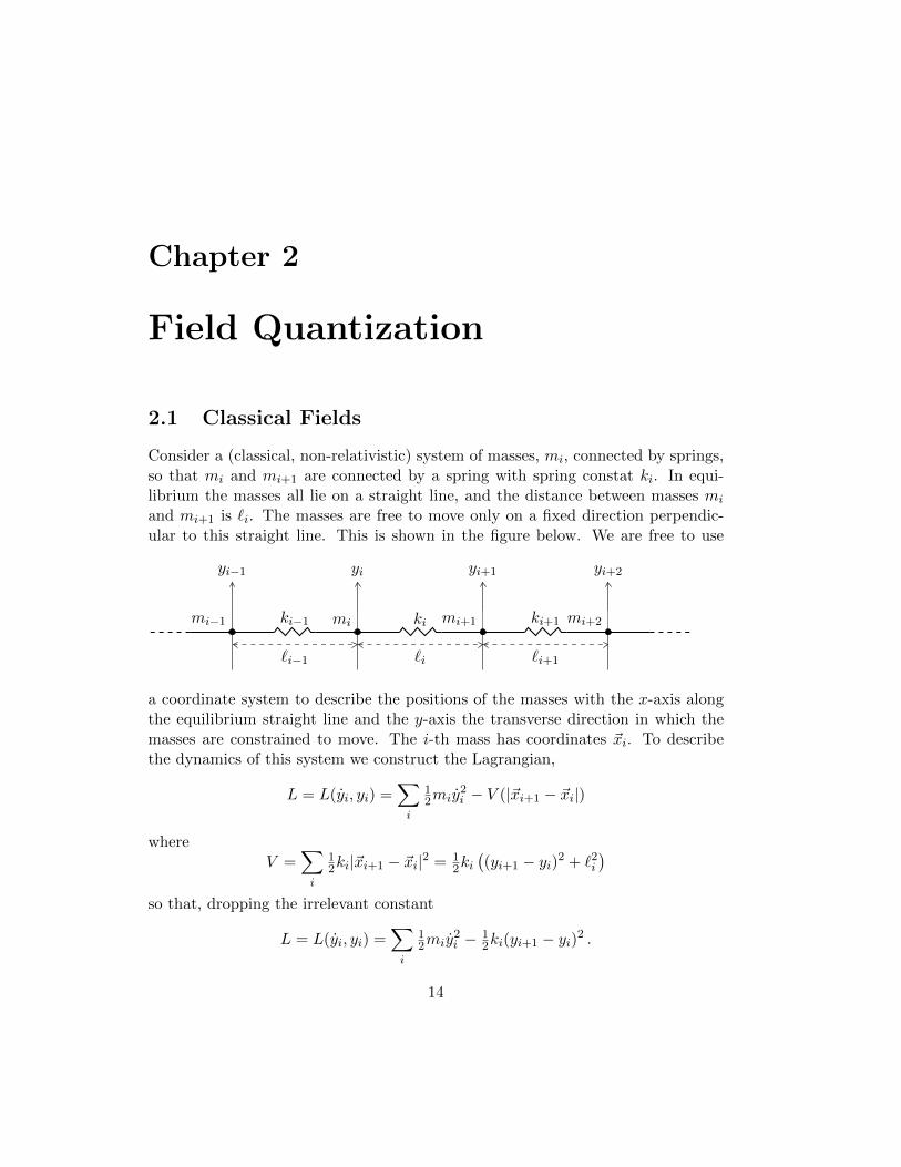
Consider a (classical, non-relativistic) system of masses, mi, connected by springs,so that mi and mi+1 are connected by a spring with spring constat ki. In equi-librium the masses all lie on a straight line, and the distance between masses mi
and mi+1 is `i. The masses are free to move only on a fixed direction perpendic-ular to this straight line. This is shown in the figure below. We are free to use
yi−1
mi−1 ki−1
yi
mi ki
yi+1
mi+1 ki+1
yi+2
mi+2
`i−1 `i `i+1
a coordinate system to describe the positions of the masses with the x-axis alongthe equilibrium straight line and the y-axis the transverse direction in which themasses are constrained to move. The i-th mass has coordinates ~xi. To describethe dynamics of this system we construct the Lagrangian,
L = L(yi, yi) =∑i
12miy
2i − V (|~xi+1 − ~xi|)
whereV =
∑i
12ki|~xi+1 − ~xi|2 = 1
2ki((yi+1 − yi)2 + `2i
)so that, dropping the irrelevant constant
L = L(yi, yi) =∑i
12miy
2i − 1
2ki(yi+1 − yi)2 .
14

2.1. CLASSICAL FIELDS 15
We are interested in this system in the limit that we cannot resolve the indi-vidual masses, so by our measuring apparatus the system appears as a continuum.Mathematically we want to take the limit `i → 0 and describe the displacement ofthe system from the x-axis at some point x along the axis, at time t, by a functionξ(x, t). This function is called a field. Since the displacement is yi at position xialong the axis, we identify yi(t)→ ξ(xi, t). Note that while xi is used classically asa coordinate of a particle, in ξ(x, t) it is just a label telling us where we are mea-suring the displacement ξ. This is an important point, so I dwell on it a bit, sincefirst time students of quantum field theory often get confused with the role of x inthe argument of a field. The field value itself can be measuring something otherthan displacement. For example, it could be temperature or pressure, or electricfield. The argument x, or in the three-dimensional case ~x of a field indicates wherethe field has a particular value. So x (or ~x) is not a dynamical variable, but ξ is.
To rewrite the Lagrangian in terms of the field, use
yi+1 − yi → ξ(xi + `i, t)− ξ(xi, t) = `i∂ξ
∂x
∣∣∣∣x=xi
+ · · · ,
where the ellipses stand for terms with higher powers of `i, and yi → ∂ξ∂t
∣∣∣x=xi
.
Multiplying and dividing by `i and interpreting `i = xi+1 − xi as the ∆x, we havethen
L =∑i
∆x
[1
2
mi
`i
(∂ξ
∂t
)2
− 1
2ki`i
(∂ξ
∂x
)2]
where the derivatives are evaluated at x = xi. We take the limit `i → 0 keeping theratio mi/`i and the product ki`i finite. These fixed ratio and product then can becharacterized with functions σ(x) and κ(x) (with σ(xi) = mi/`i and κ(xi) = ki`iin the limiting process. Of course, the sum becomes an integral and we have
L =
∫dxL =
∫dx
[1
2σ(x)
(∂ξ
∂t
)2
− 1
2κ(x)
(∂ξ
∂x
)2].
The function L = L(∂tξ, ∂xξ, ξ, x, t) is called a Lagrangian density. This is ourfirst example of a field theory. The dynamics of the field ξ(x, t) is specified by theLagrangian density
L =1
2σ(x)
(∂ξ
∂t
)2
− 1
2κ(x)
(∂ξ
∂x
)2
.
In no time we will get tired of saying “Lagrangian density” so, as is commonlydone in practice, we will improperly refer to L as a Lagrangian. The distinctionshould be clear from the context (if it is integrated it is actually a Lagrangian,

16 CHAPTER 2. FIELD QUANTIZATION
else it is a density). It should be no surprise that a dynamical variable that variescontinuously in space requires densities for its description.
We are often interested in systems that are homogeneous in space, that is,the location of the origin of the coordinate system should be irrelevant. So weimpose that the Lagrangian be invariant under a space translation x′ = x − a.The fields change into new fields ξ′(x′, t) = ξ(x, t), which is just a relabeling of thedynamical variables (a canonical transformation, to be precise). But σ(x) and κ(x)do change, unless σ(x + a) = σ(x) and κ(x + a) = κ(x) for any a. This implies,σ(x) = σ = constant and κ(x) = κ = constant. Given this, it is convenientto introduce a change of variables, φ(x, t) =
√κξ(x, t), so that the Lagrangian
density is written more simply:
L =1
2
1
c2s
(∂φ
∂t
)2
− 1
2
(∂φ
∂x
)2
. (2.1)
where we have introduced the shorthand c2s = κ/σ.
Before we go over to find the equations of motion for this system, let’s review thederivation of the Euler-Lagrange equations (or equations of motion) for a systemwith discrete degrees of freedom. Given a Lagrangian L = L(qa, qa), Hamilton’sprinciple says the equations of motion are obtained from requiring that the actionintegral be extremized:
δS[qa(t)] = δ
∫ t2
t1
dl L(qa, qa) = 0 with qa(t1) = qaini and qa(t2) = qafin
Computing we have,
0 =
∫ t2
t1
dt∑a
[∂L
∂qad
dtδqa +
∂L
∂qaδqa]
=
∫ t2
t1
dt∑a
δqa[− d
dt
∂L
∂qa+∂L
∂qa
]+∂L
∂qaδqa∣∣∣∣t2t1
The last term vanishes by the fixed boundary conditions δqa(t1,2) = 0, and the firstterm vansihes for arbitrary variation δqa(t) if
∂L
∂qa− d
dt
∂L
∂qa+ = 0
These are the Euler-Lagrange equations.Moving on to the continuum case, we apply the same principle, that the action
integral be an extremum under variations of the dynamical variable, φ(x, t):
δS[φ(x, t)] = δ
∫dtL = δ
∫ t2
t1
dt
∫dxL(∂tφ, ∂xφ, φ, t) = 0.
The boundary conditions are now φ(x, t1) = φini(x) and φ(x, t2) = φfin(x). Wehave intentionally not specified boundary conditions for the x-integration. This

2.1. CLASSICAL FIELDS 17
will allow us to decide what are reasonable conditions as we derive equations ofmotion. Computing the variation of S does not introduce new complications:
0 = δS =
∫ t2
t1
dt
∫dx
∂L
∂(∂φ∂t
) ∂δφ∂t
+∂L
∂(∂φ∂x
) ∂δφ∂x
+∂L∂φ
δφ
=
∫ t2
t1
dt
∫dxδφ
− ∂
∂t
∂L
∂(∂φ∂t
) − ∂
∂x
∂L
∂(∂φ∂x
) +∂L∂φ
+
∫dx
∂L
∂(∂φ∂t
)δφ∣∣∣t2t1
+
∫ t2
t1
dt∂L
∂(∂φ∂x
)δφ∣∣∣x=?
The first term on the last line vanishes by the boundary conditions at t = t1,2.The second term vanishes if we fix boundary conditions on φ(x, t) at the limits ofintegration for x. If the field is defined over the whole line x ∈ (−∞,∞) then wecan specify limx→±∞ φ(x, t) = 0. This is reasonable. If you start with the collectionof springs and masses form its equilibrium configuration, and poke it somewhere,it will take infinite time for the masses infinitely far away to be excited. But we areconsidering finite time, and in finite time the masses far away never get displacedfrom equilibrium. This is even clearer in the continuum case. We will see shortlythat φ satisfies a wave equation with finite speed of propagation. Alternatively,we can imagine the case of a finite system of springs and masses extending fromx = 0 to x = L. The limit of `i → 0 still requires that we take the number ofmasses and springs to infinity, but we can do so with the field confined to the regionx ∈ [0, L]. In this case we need to introduce boundary conditions at x = 0 and L.If the ends of the line of masses are fixed, then in the limit φ(0, t) φ(L, t) are fixed.Another popular setup is to have periodic boundary conditions, φ(L, t) = φ(0, t).This means the field is defined on a 1-dimensional torus (really a circle, but thegeneralization to higher dimensions is a torus). This also makes the last termsvanish. Physically, if we have only finite time and the size of the system L issufficiently large, the precise choice of boundary conditions should be irrelevant.
Setting to zero the coefficient of the arbitrary variation δφ(x, t) gives the Euler-Lagrange equations:
− ∂
∂t
∂L
∂(∂φ∂t
) − ∂
∂x
∂L
∂(∂φ∂x
) +∂L∂φ
= 0 ,
To obtain equations of motion in our example, (2.1), compute,
∂L∂φ
= 0 ,∂L
∂(∂φ∂x
) = −∂φ∂x
,∂L
∂(∂φ∂t
) =1
c2s
∂φ
∂t,

18 CHAPTER 2. FIELD QUANTIZATION
and use in the Euler-Lagrange equations:
1
c2s
∂2φ
∂t2− ∂2φ
∂x2= 0
You recognize this as the wave equation! The general solution is
φR(x− cst) + φL(x+ cst)
describing right and left moving waves with speed of propagation cs (the speed of“sound,” hence the subscript s).
Since the notation above is pretty unwieldy, we use, as previously advertised,∂t for ∂/∂t, and ∂x for ∂/∂x so that, for example, we write the Euler-Lagrangeequations as
−∂t∂L∂tφ− ∂x
∂L∂xφ
+∂L∂φ
= 0 .
Relativistic Fields In the example above we are free to take the speed of lightc = 1 for the parameter cs. The solutions to the equation of motion are waves thatpropagate at the speed of light. Is this then a Lorentz invariant theory? Yes!
We can check this by verifying that if φ(x, t) is a solution, so is φ′(x, t) ≡ φ(x′, t′)where
x′ = γ(x− βt)t′ = γ(t− βx)
γ =1√
1− β2
Alternatively, we can verify that the action integral , S =∫ ∫L dt dx, from which
the equations are derived, is itself invariant. To this end compute,
∂φ′(x, t)
∂x=∂φ(x′, t′)
∂x=∂φ(x′, t′)
∂x′∂x′
∂x+∂φ(x′, t′)
∂t′∂t′
∂x= γ
∂φ(x′, t′)
∂x′− βγ ∂φ(x′, t′)
∂t′
∂φ′(x, t)
∂t=∂φ(x′, t′)
∂x=∂φ(x′, t′)
∂x′∂x′
∂t+∂φ(x′, t′)
∂t′∂t′
∂t= −βγ ∂φ(x′, t′)
∂x′+ γ
∂φ(x′, t′)
∂t′
and use this in the Lagrangian density, (2.1) (with cs = c = 1):
L =1
2
(∂φ′(x, t)
∂t
)2
− 1
2
(∂φ′(x, t)
∂x
)2
=1
2
(∂φ(x′, t′)
∂t′
)2
− 1
2
(∂φ(x′, t′)
∂x′
)2
.
Finally integrate this over∫ ∫
dtdx to obtain the action. On the right hand side
of the equation change variables of integration , dx dt =∣∣∣ ∂(x,t)∂(x′,t′)
∣∣∣ dx′ dt′ = dx′ dt′ to
obtain finally∫ ∫dt dxL(φ′(x, t)) =
∫ ∫dt′ dx′ L(φ(x′, t′)) =
∫ ∫dt dxL(φ(x, t))
2.1. CLASSICAL FIELDS 19
where in the last step we changed the label for the dummy variables of integrationfrom (x′, t′) to (x, t). This shows invariance of the action integral, S[φ′(x, t)] =S[φ(x, t)]; the theory is Lorentz invariant.
We could have saved ourselves a lot of time had we taken advantage of the nota-tion designed to exhibit the properties of quantities under Lorentz transformations.We can rewrite the Lagrangian density
L =1
2
(∂φ(x, t)
∂t
)2
− 1
2
(∂φ(x, t)
∂x
)2
=1
2ηµν ∂µφ∂νφ =
1
2∂µφ∂µφ
As we have seen ∂µφ transforms as a vector, and the Lagrangian is just the invariantsquare of this vector!
Klein-Gordon, again While the Lagrangian density above was obtained by alimiting process from a system fo discrete masses and springs, we do not insistin interpreting the relativistic system as some collection of infinitesimal springsand masses. We can take a more general approach to writing a Lagrangian densitywhich may be a good model for some physical system by insisting it written in termsof the appropriate number and type of fields, and constraining it by principles andsymmetries we want to incorporate.
For example: Suppose we have a system in 1-spatial dimension that can bedescribed by a single field, φ(x, t). Moreover, we want it to satisfy an equationof motion of second order (no more than second time derivatives), and we wantthe action to be invariant under Lorentz transformations. Then the Lagrangiandensity, L = L(φ, ∂µφ), can include derivatives only through the invariant ∂µφ∂µφ.The simplest Lagrangian density we can think of is the one in the example above,L = 1
2∂µφ∂µφ. The next simplest is
L = 12∂
µφ∂µφ− 12m
2φ2.
We could have included also a linear term, gφ, with g a a constant, but we caneliminate that term by a field redefinition φ→ φ+g/m2. The Euler-Lagrange equa-tion that follows from this Lagrangian density is the 1-spatial dimension versionof the Klein-Gordon equation! It is instructive to derive the equation of motionanew, maintaing Lorentz covariance explicitly throughout the computation. Wefirst integrate by parts to recast the action as
S[φ] =
∫d2x
[−1
2φ∂2φ− 1
2m2φ2]
where ∂2 = ∂µ∂µ. Taking a variation is now trivial,
0 = δS = −∫d2x δφ
[∂2φ+m2φ
]

20 CHAPTER 2. FIELD QUANTIZATION
leading to (∂2 +m2
)φ(x, t) = 0
which you recognize as the Klein-Gordon equation.
2.2 Field Quantization
As we argued in the introduction we need to account for pair creation not justbecause it is a natural phenomena and because it matters for accuracy, but alsobecause it is required if we are to have a consistent relativistic quantum mechanicaltheory. We could proceed by enlarging the Hilbert space to include multi-particlestates, |~p〉, |~p, ~p ′〉 = |~p〉 ⊗ |~p ′〉, etc, and then introduce creation/annihilation oper-ators to describe interactions that change particle number. The end result is thesame as what we will obtain from tackling head on the problem of quantization offields.
Before we do so, let’s review quantization of classical systems with a discreteset of generalized coordinates qi, with i = 1, . . . , N . We are given a Lagrangian,from which conjugate momenta and a Hamiltonian follow:
L = L(qi, qi) ⇒ pi =∂L
∂qiand H = piqi − L
Poisson brackets are defined on any functions of pi and qi by
f, gP =∂f
∂qi
∂g
∂pi− ∂g
∂qi
∂f
∂pi. (2.2)
Note that here, and in the definition of the Hamiltonian, we have used the gener-alized Einstein summation convention. One has, in particular, qi, pjP = δij andqi, qjP = 0 = pi, pjP . Moreover, the equations of motion in the Hamiltonianformalism can be written as pj = pj , HP = −∂H/∂qj and qj = qj , HP =∂H/∂pj . Quantization proceeds by associating an operator on a Hilbert spaceH with each of the generalized coordinates and momenta, qi → qi and pi → pi,and replacing the Poisson bracket by (−i times) the commutator of the operators,qi, pjP = δij → −i[qi, pj ] = δij . Similarly [qi, qj ] = 0 = [pi, pj ]. Evolution ofoperators is given likewise, e.g., ipj = [pj , H] and iqj = [qj , H].
We would like to use this same method to quantize field theories. Let’s first un-derstand the analogues of conjugate momentum, Hamiltonian and Poisson bracketin classical field theory and only then quantize. Consider the 1-spatial dimensionalsystem of the previous section. How do we take the continuum limit of the Poissonbrackets, Eq. (2.2)? It is convenient to start with∑
j
qi, pjP =∑j
δij = 1

2.2. FIELD QUANTIZATION 21
For the continuum limit rewrite∑
j pj =∑
j `(pj/`), where we have taken a com-mon separation `i = ` for simplicity. This suggests pj(t) → π(x, t), some sort ofconjugate momentum density. On the right hand side of the Poisson bracket then1 =
∑j δij →
∫dx δ(x− x′). That is
φ(x), π(x′)P = δ(x− x′)
Sinceδφ(x)
δφ(x′)= δ(x− x′)
we are led to define
f, gP =
∫dx
[δf
δφ(x)
δg
δπ(x)− δg
δφ(x)
δf
δπ(x)
]The momentum conjugate to φ can be defined intrinsically (without taking a limitof the discrete system),
π =∂L∂φ
and the Hamiltonian density is defined by
H = πφ− L .
We are ready to quantize this 1+1 dimensional field theory. We introduce her-mitian operators φ and π on a Hilbert space, and use the quantization prescriptionthat gives us commutation relations from the Poisson brackets,
− i[φ(x, t), π(x′, t)] = δ(x− x′) , [φ(x, t), φ(x′, t)] = 0 = [π(x, t), π(x′, t)] (2.3)
Note that the commutation relations are given at a common time, but separatespace coordinate. The field operators satisfy equations of motion, the Euler-Lagrange equations from the Lagrangian density L. Alternatively, time evolutionis given by
i∂tπ(x, t) = [π(x, t), H] and i∂tφ(x, t) = [φ(x, t), H]
where the Hamiltonian is
H =
∫dx H .
Let’s work this out for the 1+1 Klein-Gordon example:
L = 12∂
µφ∂µφ− 12m
2φ2 .
22 CHAPTER 2. FIELD QUANTIZATION
The momentum conjugate to φ is
π =∂L∂φ
= ∂tφ
and the Hamiltonian density is
H = 12 π
2 + 12(∂xφ)2 + 1
2m2φ2 .
The quantum field equation is just the Klein-Gordon equation,
[∂2 +m2]φ(x, t) = 0 .
Alternatively,
i∂tπ(x, t) = [π(x, t), H] = −i(−∂2xφ+m2φ) and i∂tφ(x, t) = [φ(x, t), H] = iπ(x, t)
The fields satisfy the equal-time commutation relations (2.3). To understand thecontent of this theory, we Fourier expand, at fixed time, say t = 0
φ(x) =
∫dk
2πφ(k)eikx and π(x) =
∫dk
2ππ(k)eikx.
That t = 0 is implicit here and in the next few lines. Since φ†(x) = φ(x) wehave φ(k)† = φ(−k) and π(k)† = π(−k). The equal-time commutation relations[φ(x), φ(x′)] = 0 and [π(x), π(x′)] = 0 imply
[φ(k), φ(k′)] = 0 = [π(k), π(k′)]
Then [φ(x), π(x′)] = iδ(x− x′) gives
iδ(x− x′) =
∫dk
2π
∫dk′
2π
[φ(k)eikx, π(k′)eik
′x′]⇒ [φ(k), π(k′)] = 2πiδ(k + k′)
The advantage of Fourier transforming shows up first in computing the Hamilto-nian, since the ∂2
x term is diagonalized:
H =
∫dk
2π
[12 π†(k)π(k) + 1
2(k2 +m2)φ†(k)φ(k)]
=
∫dk
2π
[12 π†(k)π(k) + 1
2ω2kφ†(k)φ(k)
]I have written ωk for the energy ωk = Ek =
√k2 +m2 for two reasons: (i) we have
not shown that k is a momentum so we have no right yet to think of√k2 +m2 as
the energy, and (ii) it becomes clear that the expression for H is that of an infinitesun of linear harmonic oscillators, H = 1
2 p2 + 1
2ω2q2.
2.2. FIELD QUANTIZATION 23
Review of QM-simple harmonic oscillator Consider the spring mass systemdescribed by
L = 12 q
2 − 12ω
2q2
Correspondingly
H = 12p
2 + 12ω
2q2
Here q and p, aas well as H, are operators on the Hilbert space, but we are sup-pressing the hat over the symbols since there will be no occasion for confusion:
i[p, q] = 1
Let
a =1√2ω
(ωq + ip)
a† =1√2ω
(ωq − ip)
Then a†a = 1/2ω(ω2q2 + p2 − iω[p, q]) = 1/2ω(2H − ω) or
H = ω(a†a+ 12)
Moreover, [a, a†] = 12ω [ωq + ip, ωq − ip] = 1
2ω (2iω)[p, q] so we have
[a, a†] = 1
[a, a] = 0
[a†, a†] = 0
and then
[H, a†] = ωa†
[H, a] = −ωa
We can use these to find the spectrum. Assume that the state |E〉 is an energyeigenstate:
H|E〉 = E|E〉
Then
H(a†|E〉) = (E + ω)(a†|E〉
)

24 CHAPTER 2. FIELD QUANTIZATION
which means |E + ω〉 = N+a†|E〉 for some normalization constant, N+. If |E〉 is
normalized, 〈E|E〉 = 1, then
1 = 〈E + ω|E + ω〉 = |N+|2〈E|aa†|E〉
= |N+|2〈E|(
[a, a†] + a†a)|E〉
= |N+|2〈E|(
1 +1
2ω(2H − ω) + a†a
)|E〉
= |N+|2(E
ω+
1
2
)Similarly, |E − ω〉 = N−a|E〉 and
1 = 〈E − ω|E − ω〉 = |N−|2〈E|a†a|E〉 = |N−|2(E
ω+
1
2
)So we have an infinite tower of states with energies E, E ± ω, E ± 2ω, . . . Sincethe operators a† and a raise and lower energies, we call them raising and loweringoperators, respectively. To avoid a spectrum that is unbounded from below (acatastrophic instability once the system is coupled to external forces), we can insistthat for some state |0〉 the tower stops:
a|0〉 = 0
This is the minimum energy state, the “ground state.” It has energy H|0〉 = 12ω|0〉,
called the “zero-point” energy. Then a†|0〉 has energy E1 = ω+ω2 and so on, (a†)n|0〉
has energy En = ω(n+ 12). The tower of states then can be labeled by an integer,
|En〉 = |n〉. We assume they are normalized. Then, from above, |n+ 1〉 = N+a†|n〉
with
|N+|−2 =Enω
+1
2= n+ 1
so that
|n+ 1〉 =1√n+ 1
a†|n〉 =1√
(n+ 1)n(a†)2|n− 1〉 = · · · = 1√
(n+ 1)!(a†)n+1|0〉
Note that since aa† = a†a + 1 one has 12ω(aa† + a†a) = 1
2ω(2a†a + 1) = H. Thisway of writing H = 1
2ω(aa† + a†a) hides the zero-point energy.
2.2.1 Particle Interpretation
This suggests introducing
ak =1√2π
1√2ωk
(ωkφ(k) + iπ(k)
)a†k =
1√2π
1√2ωk
(ωkφ(k)† − iπ(k)†
) (2.4)
2.2. FIELD QUANTIZATION 25
These have[ak, a
†k′ ] = δ(k − k′)
[ak, ak′ ] = 0
[a†k, a†k′ ] = 0
(2.5)
where we have used ω−k = ωk. To compute the Hamiltonian, note that
a†kak =1
4πωk
(ω2kφ(k)†φ(k) + π(k)†π(k)− iωkπ(k)†φ(k) + iωkφ(k)†π(k)
). (2.6)
Since we are going to sum over∫dk, we can change variables k → −k in the last
term,1
4πωkiωkφ
†(k)π(k)→ i
4πφ†(−k)π(−k) =
i
4πφ(k)π(−k)
The first two terms in (2.6) are the Hamiltonian density and the last two combineinto a commutator, so we have
H =1
2
∫dk
2π
(π(k)†π(k) + ω2
kφ(k)†φ(k))
=1
2
∫dk
2π
(4πωka
†kak + ωki[π(k)†, φ(k)]
)=
∫dk(ωka
†kak + ωkδ(0)
)=
1
2
∫dkωk
(a†kak + aka
†k
)Let’s examine what we have. Assuming that there is a ground state such that
ak|0〉 = 0 for all k, we have a Hilbert space obtained by acting with a†k’s on |0〉,e.g.,
(a†k1)n1(a†k2)n2 · · · )|0〉 . (2.7)
The ground state |0〉 has energy E0 given by
H|0〉 =
∫dk′ ωk′
(a†k′ak′ + δ(0)
)|0〉 =
∫dk′ ωk′δ(0)|0〉 ≡ E0|0〉 ,
and the state |k〉 = a†k|0〉 has energy
H|k〉 =
∫dk′ ωk′
(a†k′ak′ + δ(0)
)|k〉 = (ωk + E0)|k〉
While the zero-point energy, E0, is infinite, the difference of energy between thestate |k〉 and the ground state is well defined, finite, ∆E = ωk. The same is trueof the energy of any of the states (2.7). We can only measure energy differences

26 CHAPTER 2. FIELD QUANTIZATION
(except in gravitation; that’s another story). That is, we are free to add a constantto H without changing the physical content of the theory. So we can redefine
H =
∫dk ωka
†kak
Examining this more closely write
H =1
2
∫dk ωk
(a†kak + aka
†k − 〈0|a
†kak + aka
†k|0〉
)=
∫dk ωka
†kak .
We say that in the new expression the operators a†k and ak appear “normal ordered”and the operation is called “normal ordering” or “Wick ordering:”
:12(a†kak + aka
†k): ≡ a
†kak .
Under :ξ: the operators in ξ commute. The computation above uses the groundstate for reference. We will need to make sure that this procedure preserves Lorentzinvariance. More on this later.
The energy of the state |k〉 is Ek = ωk =√k2 +m2. So we identify p = k
the momentum of the state. This is just as in our introductory presentation ofrelativistic QM for a single non-interacting particle. This is then interpreted as asingle particle state. But now the theory is much richer. For one thing we havemany other states, as in (2.7). The Hilbert space of states in (2.7) is called a “Fockspace.” We interpret them as many particle states. To see this we check a fewthings:
(i) Energy of (a†k1)n1(a†k2)n2 · · · |0〉 is E = n1Ek1 + n2Ek2 + · · ·
(ii) Momentum of (a†k1)n1(a†k2)n2 · · · |0〉 is p = n1k1 + n2k2 + · · ·
The first one follows trivially from the expression for H and its action on the statesin (2.7). For the second we introduce the operator
p =
∫dk k a†kak
which gives the desired eigenvalues. We will verify this is the momentum operatorbelow.
From now on we call the operators a†k and ak creation and annihilation oper-ators, respectively, rather than raising and lowering operators, to remind us thatthey are adding or taking away a particle from a state. The ground state, |0〉 isparticleless, so we call it the vacuum state or just the vacuum.

2.2. FIELD QUANTIZATION 27
Statistics As promised, that particles are identical is an automatic consequenceof QFT. Note that all particles have the same mass. Moreover, the multiple particlestates are automatically symmetric. For example, let |k1, k2〉 = a†k1a
†k2|0〉. Then
|k1, k2〉 = a†k1a†k2|0〉 = a†k2a
†k1|0〉 = |k2, k1〉
where we have used the commutation relations (2.5). More generally |k1, . . . , kn〉is symmetric under exchange of any ki’s. This is an unexpected surprise! InNR-QM one simply assumes the wave function is symmetric for bosons (Bose-Einstein statistics), anti-symmetric for fermions (Fermi-Dirac statistics), and it isobserved empirically that integer-spin particles are bosons while half-integer spinparticles are fermions. There was a hidden assumption in our calculation thatresulted in bosonic particles. The assumption is that quantization goes through thereplacement p, qP → i[p, q]− = i(pq− qp) rather than p, qP → i[p, q]+ = i(pq+ qp).We will later see that a consistent formulation of QFT requires we use [ , ]− forinteger spin fields and [ , ]+ for half-integer spin fields. So not only we will getidentical particles automatically, we will get the correct assignment automaticallytoo:
• bosons: spin-0, 1, . . .
• fermions: spin-12 , 3
2 , . . .
Normalization Note also that
〈k|k′〉 = 〈0|aka†k′ |0〉 = 〈0|[ak, a†k′ ]|0〉 = δ(k − k′)
〈k1, k2|k′1, k′2〉 = 〈0|ak1ak2a†k′1a†k′2|0〉 = δ(k1 − k′1)δ(k2 − k′2) + δ(k1 − k′2)δ(k2 − k′1)
exactly what we expect of identical particle plane wave states. But this is not thedesired relativistic normalization. Not a problem, we only need to take for thedefinition of states
|k〉 =√
(2π)(2Ek)a†k|0〉 ⇒ 〈k|k′〉 = (2π)2Ekδ(k − k′)
Plane waves are not normalizable states, but we can make normalizable wavepackets out of them:
|ψ〉 =
∫dk ψ(k)a†k|0〉 ⇒ 〈ψ|ψ〉 =
∫dk dk′ ψ(k)∗ψ(k′)〈0|aka†k′ |0〉 =
∫dk |ψ(k)|2 <∞
It is often convenient to define creation and annihilation operators by rescalingthe ones we have:
αk =√
(2π)(2Ek)ak

28 CHAPTER 2. FIELD QUANTIZATION
so that |k〉 = αk|0〉 has relativistic normalization. In terms of these
H =
∫(dk)Ekα
†kαk
p =
∫(dk) kα†kαk
where (dk) is the relativistic invariant measure.
Number Operator The state with n-particles is an energy Eigenstate. It there-fore evolves into a state with n particles (itself). Particle number is conservedbecause there are no interactions (yet). This suggest there must be an observable,that is, a hermitian operator, N that
(i) is conserved , [N , H] = 0
(ii) 〈ψ|N |ψ〉 = N , the number of particles in state ψ (if it has a definite numberof particles)
It should be obvious by now that
N =
∫dk a†kak =
∫(dk)α†kαk
satisfies the above conditions.We will see later how to generalize these statements to when we include in-
teractions. The startegy will be to derive the form of pµ and N from conservedcurrents associated with symmetries of L.
Time evolution We have quantized at t = 0. In the Heisenberg representationfields have time dependence. So consider φ(x, t), with φ(x, 0) corresponding tothe field we denoted by φ(x) at t = 0 above. Note that the initial choice t = 0is arbitrary since we have time translation invariance (the Lagrangian does notdepend explicitly on time). Now,
∂tφ(x, t) = π(x, t) = i[H, φ(x, t)] .
The solution is well known,
φ(x, t) = eiHtφ(x)e−iHt .
To understand how this operator acts on the Fock space we cast it in terms ofcreation and annihilation operators. To this end we invert (2.4)
αk = ωkφ(k) + iπ(k)
α†−k = ωkφ(k)− iπ(k)⇒
φ(k) =1
2ωk
(αk + α†−k
)π(k) = − i
2ωk
(αk − α†−k
)

2.2. FIELD QUANTIZATION 29
Hence
φ(x) =
∫(dk)
(αke
ikx + α†ke−ikx
).
The time dependence is now straightforward:
φ(x, t) = eiHtφ(x)e−iHt =
∫(dk)
(αke
−iEkt+ikx + α†keiEkt−ikx
)=
∫(dk)
(αke
−ik·x + α†keik·x),
where in the last line we have introduced kµ = (E, k) and xµ = (t, x) to makerelativistic invariance explicit. Clearly H, p and N are time independent; this iseasily seen by taking αk → e−iEktαk in the expressions for H, p and N). Noe thepresence of positive and negative energies in φ(x, t). But there are no “negativeenergy states.” Instead there are annihilation operators that subtract honestlypositive energies form states, and creation operators that add it.
Note that the field φ(x, t) satisfies the equation of motion,(∂2t − ∂2
x +m2)φ(x, t) = 0
This should be the case, as expected from the commutation relations ∂tπ = i[H, π]and ∂tφ = i[H, φ]. But we can verify this directly from the expansion in creationand annihilation operators using
(∂2t − ∂2
x)e−iEkt+ikx = −(E2k − k2)e−iEkt+ikx = −m2e−iEkt+ikx ,
or in relativistic notation,
∂2e−ik·x = −k2e−ik·x = −m2e−ik·x .
Momentum Operator We would like the momentum operator to be definedso that ip generates translations (and is conserved). We have already defined theoperator, so we check now that it does what we want:
[p, φ(x, t)] =
∫(dk′)(dk)
[k′α†k′αk′ , αke
−iEkt+ikx + α†keiEkt−ikx
]=
∫(dk)k
(−αke−iEkt+ikx + α†ke
iEkt−ikx)
= i∂x
∫(dk)
(αke
−iEkt+ikx + α†keiEkt−ikx
)= i∂xφ(x, t) .
Moreover,[p, H] = 0
so p is a constant in time, that is, it is conserved.

30 CHAPTER 2. FIELD QUANTIZATION
Causality While the vanishing of the equal-time commutation relation,[φ(x′, 0), φ(x, 0)] = 0, was assumed from the start, there is no reason to suspect ananalogous result for non-equal times. Let’s compute,
[φ(x, t), φ(x′, t′)] =
∫(dk)(dk′)
[αke
−ik·x + α†keik·x, αk′e
−ik′·x′ + α†k′eik′·x′
]=
∫(dk)
(eik·(x
′−x) − e−ik·(x′−x))
(2.8)
Notice that the right hand side is explicitly Lorentz invariant and only a functionof the difference of 2-vectors, x′ − x. We define
i∆(x′ − x) = [φ(x, t), φ(x′, t′)] .
Using Lorentz invariance it is easy to prove that ∆(x) = 0 for space-like x. Since∆(x) is Lorentz invariant we can compute it in a boosted frame. For space-like xthere is a boost that sets t = 0, that is, for space-like separation x′ − x there is aframe for which t′ = t. The commutator vanishes at equal times, and we can thenboost back to the original frame to obtain ∆(x) = 0 for x2 < 0. It is not difficultto verify this from the integral above by explicit calculation. One assumes x2 < 0and continues the integral of the first term in (2.8) much as was done in Fig. 1.1.The second term is continued along a contour on the lower half plane. The twoterms cancel each other.
As promised causality is restored. The contribution of the positive and negativeenergy states cancelled each other. Only, there are no negative energy states. Thereare annihilation operators.
2.3 3 + 1 Dimensions
Remarkably little changes as we move on to discuss the case of 3 pace and 1 timedimensions. Now
L(t) =
∫d3xL =
∫d3x
[12(∂µφ)2 − 1
2m2φ2],
where the equality is general and the second gives the explicit case of the Lagrangianfor Klein-Gordon theory. We have used φ = φ(~x, t) = φ(xµ), often also denoted asφ(x), and (∂µφ)2 = ηµν∂µφ∂νφ (sometimes also denoted as (∂φ)2, we really like tocompress notation). The Poisson brackets are as before, replacing δ(3)(~x′ − ~x) forδ(x′−x). This goes over directly into the quantum version. So we have equal timecommutation relations
− i[φ(~x, t), π(~x′, t)] = δ(3)(~x− ~x′) , [φ(~x, t), φ(~x′, t)] = 0 = [π(~x, t), π(~x′, t)](2.9)

2.3. 3 + 1 DIMENSIONS 31
As before these are solved by
φ(~x, 0) =
∫(dk)
[α~kei~k·~x + α†~k
e−i~k·~x]
π(~x, 0) = −i∫
(dk)E~k
[α~kei~k·~x − α†~ke
−i~k·~x]
with
[α~k , α†~k ′
] = (2π)32E~kδ(3)(~k − ~k ′)
[α~k , α~k ′ ] = 0 = [α†~k, α†~k ′
]
and these are interpreted as annihilation and creation operators for relativisticallynormalized particle states with mass m: if the vacuum state is |0〉 then
|~k〉 = α†~k|0〉 has 〈~k |~k ′〉 = (2π)32E~kδ
(3)(~k − ~k ′) .
After normal ordering the Hamiltonian is
H =
∫(dk)E~k
α†~kα~k.
The conserved operator
N =
∫(dk)α†~k
α~k.
counts number of particles and
~p =
∫(dk)~k α†~k
α~k.
are the conserved momentum operators and generate translations. As before theparticles are identical and multiplarticle states satisfy Bose-Einstein statistics. Incontrast to the 1+1 case, in 3-spatial dimensions we can speak meaningfully of thespin of a particle. It must correspond to a quantum number that transforms underrotations. Our field is invariant under Lorentz transformations, φ(x) → φ′(x) =φ(x′), where x′ = Λx, and this is results in spinless particles. The spin-statisticsconnection comes out automatically: spin-0 identical particles satisfy Bose-Einsteinstatistics.
Time evolution is still given by
φ(x) = φ(~x, t) = eiHtφ(~x, 0)e−iHt
=
∫(dk)
[α~kei~k·~x−iE~kt + α†~k
e−i~k·~x+iE~kt
]=
∫(dk)
[α~ke−ik·x + α†~k
eik·x]
32 CHAPTER 2. FIELD QUANTIZATION
where k0 = E~k. The operator φ(x) satisfies the Klein-Gordon equation,(∂2 +m2
)φ(x) = 0
which is the Euler-Lagrange equation for the Lagrangian density given above.We will encounter later the product φ(x1)φ(x2), and we will need its relation to
the normal ordered product : φ(x1)φ(x2) : . It is convenient to introduce “positiveand negative frequency operators,”
φ(−)(x) =
∫(dk)eik·xα†~k
,
φ(+)(x) =
∫(dk)e−ik·xα~k
.
Then
φ(x1)φ(x2) =(φ(+)(x1) + φ(−)(x1)
)(φ(+)(x2) + φ(−)(x2)
)= φ(+)(x1)φ(+)(x2) + φ(+)(x1)φ(−)(x2) + φ(−)(x1)φ(+)(x2) + φ(−)(x1)φ(−)(x2)
= φ(+)(x1)φ(+)(x2) + φ(−)(x2)φ(+)(x1) + φ(−)(x1)φ(+)(x2)
+ φ(−)(x1)φ(−)(x2) + [φ(+)(x1), φ(−)(x2)]
= :φ(x1)φ(x2): + [φ(+)(x1), φ(−)(x2)]
Hence the difference between the product and the normal ordered product is ac-number,
∆+(x2 − x1) ≡ [φ(+)(x1), φ(−)(x2)]
=
∫(dk1)(dk2) eik1·x1−ik2·x2 [α~k1
, α†~k2]
=
∫(dk) e−ik·(x2−x1) . (2.10)
That ∆+ is only a function of the difference is the result of the explicit calculationabove. You may recognize this as the integral in (1.1). Note that(
∂2 +m2)
∆+(x) = 0 for x 6= 0,
so ∆+(x) is a solution of the Klein-Gordon equation that does not vanish forspacelike argument.
Quantum theory is weird, of course, but QFT is even weirder. Consider this.The expectation value of φ(x) in the vacuum state is zero at any point x,
〈0|φ(x)|0〉 = 0

2.3. 3 + 1 DIMENSIONS 33
But the expectation value of the square φ2(x) is infinite:
〈0|φ2(x)|0〉 = ∆+(0) =
∫(dk) .
Fluctuations of quantum fields at any point are wild, even for the simplest emptystate! The problem arises from localization: we should not insist in determiningthe field precisely in an arbitrarily small region of space (in this case, one point).In homework you will show that the square remains finite for the field smearedover a region.

Chapter 3
Symmetries
A famous theorem of Wigner shows that symmetries in a quantum theory mustcorrespond to either unitary or anti-unitary operators. It seems fit to start witha review of what is meant by this. We will then proceed to study continuoussymmetries, all represented by unitary operators. We will then turn our attentionto discrete symmetries. It is then, in presenting time-reversal symmetry, that wewill encounter anti-unitary operators.
3.1 Review of unitary and anti-unitary operators
The bra/ket notation is not quite suitable for anti-linear operators. So for thissection we use the following notation:
• States are denoted by wave-functions: ψ, χ, . . .
• c-numbers are lowercase latin letters: a, b, . . .
• Operators are uppercase: A,B, . . . , U, V, . . . ,Ω, . . .
• Inner product and norm: (ψ, χ) and ‖ψ‖2 = (ψ,ψ)
An operator A is linear if A(aψ + bχ) = aAψ + bAχ. The hermitian conjugate A†
of an operator A, is such that for all χ, ψ
(χ,A†ψ) = (Aχ,ψ) .
This is consistent only if A is linear:
(A(aψ + bχ), ρ) = (aψ + bχ,A†ρ)
= a∗(ψ,A†ρ) + b∗(χ,A†ρ)
= a∗(Aψ, ρ) + b∗(Aχ, ρ)
= (aAψ + bAχ, ρ)
34

3.1. REVIEW OF UNITARY AND ANTI-UNITARY OPERATORS 35
for any ρ.An invertible operator U is unitary if
(Uψ,Uχ) = (ψ, χ) (and therefore ‖Uψ‖ = ‖ψ‖).
Unitary operators are linear. Proof:
‖U(aψ + bχ)− aUψ − bUχ‖2 = ‖U(aψ + bχ)‖2−2Re [a(U(aψ + bχ), Uψ)]
− 2Re [b(U(aψ + bχ), Uχ)] + |a|2 ‖Uψ‖2 +|b|2 ‖Uχ‖2
= ‖aψ + bχ‖2−2Re [a(aψ + bχ, ψ)]
− 2Re [b(aψ + bχ, χ)] + |a|2 ‖ψ‖2 +|b|2 ‖χ‖2
= 0
where we have used unitarity in going form the first to the second line and we haveexpanded all terms in going from the second to the third line. Since only zero haszero norm we have U(aψ+ bχ)−aUψ− bU = 0, completing the proof. The inverseof a unitary operator is its hermitian conjugate:
(ψ,U−1χ) = (Uψ,U(U−1χ)) = (Uψ, χ) = (ψ,U †χ)
for any ψ, χ.An invertible operator Ω is anti-unitary if for all ψ, χ
(Ωψ,Ωχ) = (χ, ψ) (notice inverted order).
An operator Bis anti-linear if for all ψ, χ
B(aψ + bχ) = a∗ Bψ + b∗ Bχ
Anti-unitary operators are anti-linear. The proof is the same as in linearity ofunitary operators, ‖Ω(aψ + bχ) − a∗Ωψ + b∗Ωχ‖2 = 0. Example: the complexconjugation operator, Ωc. Clearly
Ωc(aψ + bχ) = a∗Ωcψ + b∗Ωcχ and (Ωcψ,Ωcχ) = (χ, ψ) .
You can show that the products U1U2 and Ω1Ω2 of two unitary or two anti-unitary operators are unitary operators, while the products UΩ and ΩU of a unitaryand an anti-unitary operators are anti-unitary.
Symmetries What properties are required of operator symmetries in QM? If Ais an operator on the Hilbert space, F = ψ, then it is a symmetry transformationif it preserves probabilities, |(Aψ,Aχ)|2 = |(ψ, χ)|2. Wigner showed that the onlytwo possibilities are A is unitary or anti-unitary.

36 CHAPTER 3. SYMMETRIES
Symmetry transformations as action on operators: for unitary operators, thesymmetry transformation ψ → Uψ, for all states, gives
(ψ,Aχ)→ (Uψ,AUχ) = (ψ,U †AUχ)
So we can transform instead operators, via A→ U †AU . For anti-unitary operatorsthe hermitian conjugate is not defined, so we do not have “Ω† = Ω−1”. But
(ψ,Aχ)→ (Ωψ,AΩχ) = (Ω−1AΩχ,Ω−1Ωψ) = (ψ, (Ω−1AΩ)†χ) ,
which is not very useful. For expectation values of observables, A† = A,
(ψ,Aψ)→ (Ωψ,AΩψ) = (AΩψ,Ωψ) = (ψ,Ω−1AΩψ)
and in this limited sense, A→ Ω−1AΩ.
3.2 Continuous symmetries, Generators
Consider a family of unitary transformations, U(s), where s is a real number in-dexing the unitary operators. We assume U(0) = 1, the identity operator. Fur-thermore, assume U(s) is continuous, differentiable. Then expanding about zero,
U(ε) = 1 + iεT +O(ε2) (3.1)
U(ε)†U(ε) = 1 = (1− iεT †)(1 + iεT ) +O(ε2) ⇒ T † = T (3.2)
iT ≡ dU(s)
ds
∣∣∣∣s=0
(3.3)
The operator T is called a symmetry generator.Now, the product of N transformations is a transformation, so consider(
1 + is
NT)N
In the limit N →∞,(1 + i sN T
)is unitary , and therefore so is
(1 + i sN T
)N. This
is a vulgarized version of the exponential map,
U(s) = limN→∞
(1 + i
s
NT)N
= eisT .
Note thatU(s)†U(s) = e−isT eisT = 1 ,
as it should. Also, A→ U(s)†AU(s) becomes, for s = ε infinitesimal,
A→ A+ iε[A, T ] or δA = iε[A, T ] .

3.3. NOETHER’S THEOREM 37
A symmetry of the Hamiltonian has
U(s)†HU(s) = H ⇒ [H,T ] = 0 .
Since for any operator (in the Heisenberg picture)
idA
dt= [H,A] + i
∂A
∂t
we have that a symmetry generator T is a constant, dT/dt = 0 (T (t) has noexplicit time dependence). Conversely a constant hermitian operator T defines asymmetry:
dT/dt = 0 ⇒ [H,T ] = 0 ⇒ e−isTHeisT = H .
Let’s connect this to symmetries of a Lagrangian density (or, more precisely, ofthe action integral).
3.3 Noether’s Theorem
Consider a Lagrangian L(t) =∫d3xL(φa, ∂µφ
a), where the Lagrangian density isa function of N real fields φa, a = 1, . . . , N . We investigate the effect of a putativesymmetry transformation
φa → φ′a = φa + δφa, where δφa = εDabφb,
with ε an infinitesimal parameter and (Dφ)a = Dabφb is a linear operator on thecollection of fields (and may contain derivatives). Consider then L(φ′a, ∂µφ
′a).Suppose that by explicit computation we find
δL = L(φ′)− L(φ) = ε∂µFµ ,
that is, that the variation of the Lagrangian density vanishes up to a derivative, thedivergence of a four-vector. We do not require that the variation of L vanishes sincewe want invariance of the action integral, to which total derivatives contribute onlyvanishing surface terms. For any variation δφ, not necessarily of the form displayedabove,
δL =∂L∂φa
δφa +∂L
∂(∂µφa)∂µδφ
a .
If φa are solutions to the equations of motion, the first term can be rewritten andthe two terms combined,
δL = ∂µ
(∂L
∂(∂µφa)
)δφa +
∂L∂(∂µφa)
∂µδφa = ∂µ
(∂L
∂(∂µφa)δφa).

38 CHAPTER 3. SYMMETRIES
Using the variation that by assumption vanishes up to a total derivative we have
∂µFµ = ∂µ
(∂L
∂(∂µφa)Dabφb
)so that
Jµ =∂L
∂(∂µφa)Dabφb −Fµ satisfies ∂µJ
µ = 0 .
This is Noether’s theorem. Note that this can be written in terms of a generalizedmomentum conjugate, Jµ = πaµD
abφb − Fµ. Since Jµ is a conserved current, thespatial integral of the time component is a conserved “charge,”
T =
∫d3xJ0 has
dT
dt= 0 .
The conserved charge is nothing but the generator of a continuous symmetry. Wecan show from its definition that it commutes with the Hamiltonian.
Let’s look at some examples:
Translations The transformation is induced by xµ → xµ + εaµ. Clearly
δL = εaµ∂µL ⇒ Fµ = aµL .
But L = L(x), is a function of xµ only through its dependence on φa(x), so
δφa = εaµ∂µφa ⇒ Jµ(a) = πaµaν∂νφ
a − aµL = aν(πaµ∂νφa − ηµνL) .
Since aν is arbitrary, we can choose it to be alternatively along the direction ofany of the four independent directions of space-time, and we then have in fact fourindependently conserved currents:
Tµν = πaµ∂νφa − ηµνL
This is the energy and momentum tensor, also known as the stress-energy tensor.The first index refers to the conserved current and the second labels which of thefour currents.
The conserved “charges” are
Pµ =
∫d3xT 0µ .
They are associated with the transformation x → x + a and hence they are mo-menta. For example,
P 0 =
∫d3x(πaφa − L) =
∫d3xH = H

3.3. NOETHER’S THEOREM 39
as expected.Example: In our Klein-Gordon field theory
L = 12(∂µφ)2 − 1
2m2φ2 (3.4)
πµ =∂L
∂(∂µφ)= ∂µφ (3.5)
⇒ Tµν = ∂µφ∂νφ− ηµνL (3.6)
We can verify this is conserved, by using equations of motion,
∂µTµν = ∂2φ∂νφ+ ∂µφ∂ν∂µφ− ∂ν(1
2(∂µφ)2 − 12m
2φ2)
= −m2φ∂νφ+ ∂µφ∂ν∂µφ− ∂µφ∂ν∂µφ+m2φ∂νφ
= 0
Turning to the case of quantum filed theory compute now the conserved 4-momentumoperator in terms of creation and annihilation operators. For the temporal compo-nent, P 0 = H, the computation was done in the previous chapter. For the spatialcomponents we have
P i =
∫d3xT 0i =
∫d3x (π∂iφ− η0iL) =
∫d3xπ∂iφ
so that
P i =
∫d3x ∂tφ∂
iφ
=
∫d3x
∫(dk′)(dk) [(−iE~k ′)(α~k ′e
−ik′·x − α†~k ′eik′·x)][(−iki)(α~k e
−ik·x − α†~keik·x)]
=
∫(dk′)(dk) (−iE~k ′)(−ik
i)[(
(2π)3δ(3)(~k ′ + ~k )α~k ′α~k e−i(E~k ′+E~k )t + h.c.
)−(
(2π)3δ(3)(~k ′ − ~k )α~k ′α†~ke−i(E~k ′−E~k )t + h.c.
)]=
1
2
∫(dk)ki
[α~kα−~ke
−2iE~kt + α†~kα†−~ke2iE~kt + α†~k
α~k + α~kα†~k
]In the last line the first two terms are odd under ~k → −~k so they vanish uponintegration and we finally have
P i =
∫(dk) 1
2ki(α†~kα~k + α~kα
†~k
)=
∫(dk)kiα†~k
α~k .
It follows that[~P , α†~k
] = ~kα†~kso that Pµ|~k 〉 = kµ|~k 〉 .

40 CHAPTER 3. SYMMETRIES
More generally, we compute the commutator of Pµ and φ(~y , t). Since Pµ is timeindependent we can always choose to compute at equal times. Then the equal timecommutator is fixed by the commutation relations from canonical quantization:
[P i, phi(x)] =
∫d3x [π∂iφ(~x, t), φ(~y , t] = −i∂iφ(~y , t) .
The case for P 0 is a bit more involved, but we know P 0 = H so we know the resultwithout need to compute. It follows that
U(a)φ(x)U(a)† = eia·Pφ(x)e−ia·P = φ(x) + iaµ[Pµ, φ(x)] + · · · = φ(x+ a)
or φ′(x) = U(a)†φ(x)U(a) = φ(x− a).
Lorentz Transformations The transformation of states was introduced earlier,U(Λ)|~p〉 = |Λ~p〉. Assuming the vacuum state is invariant under Lorentz trans-
formations we then may take U(Λ)α†~pU(Λ)† = α†Λ~p and U(Λ)α~pU(Λ)† = αΛ~p .Therefore
U(Λ)φ(x)U(Λ)† = φ(Λx) or U(Λ)†φ(x)U(Λ) = φ(Λ−1x)
Let Λµν = δµν + εωµν with ε infinitesimal. Then ωµν = −ωνµ, and thereforehas 4 × 3/2 = 6 independent components, three for rotations (ωij) and three forboosts (ω0i). We assume L = L(φ, ∂µφ) is Lorentz invariant. What does thismean? For scalar fields φ(x) → φ′(x) = φ(Λ−1x) = φ(x′) and by the chain rule∂µφ(x′) = ∂µx
′λ∂′λφ(x′) = (Λ−1)λµ∂′λφ(x′) = Λµ
λ∂′λφ(x′), which gives
L(φ, ∂µφ)→ L′ = L(φ′(x), ∂µφ′(x)) = L(φ(x′), ∂µφ(x′)) = L(φ(x′),Λµ
λ∂′λφ(x′)) .
Invariance means L′ has the same functional dependence as L but in terms of x′,that is, L is a scalar, L(x)→ L′(x) = L(x′). This gives
L(φ(x′),Λµλ∂′λφ(x′)) = L(φ(x′), ∂′µφ(x′)) .
For example, ηµν∂µφ∂νφ → ηµνΛµλΛν
σ∂′λφ∂′σφ = ηλσ∂′λφ∂
′σφ works, but not so
aµ∂µφ for constant vector aµ since aµ does not transform (it is a fixed constant).We assume L is Lorentz invariant and compute:
δφ = φ(xµ − εωµνxν)− φ(xµ) = −εωµνxν∂µφ = −εωµνxν∂µφδL = −εωµνxν∂µL = − [∂µ(εωµνxνL)− εωµνηµνL] = −∂µ(εωµνxνL)
and then the conserved currents are
Jµ(ω) = −πµωλσxσ∂λφ+ ωµνxνL
= −ωλσ(πµxσ∂λφ− δµλxσL)

3.3. NOETHER’S THEOREM 41
or, since ωµν is arbitrary, we have six conserved currents,
Mµνλ = (πµxν∂λ − ηµλxνL)− ν ↔ λ
= xνTµλ − xλTµν .
This has
Mνλ =
∫d3xM0νλ
as generator of rotations (M ij) and boosts (M0i).Comments:
(i) The expression for Mµνλ is specific for scalar fields since we have usedU †(Λ)φ(x)U(Λ) = φ(Λ−1x). This defines scalar fields. We expect, for ex-ample, that a vector field, Aµ(x) will transform like ∂µφ(x),
U †(Λ)Aµ(x)U(Λ) = ΛµλAλ(Λ−1x) or U(Λ)†Aµ(x)U(Λ) = ΛµλA
λ(Λ−1x)
Then
δAµ = (δµν + εωµν)A(xλ − εωλσxσ)−Aµ(x)
= −ε[ωλσx
σ∂λAµ︸ ︷︷ ︸
as before
− ωµνAν︸ ︷︷ ︸
new term
]This then gives a new term in Jµ(ω) of the form ∂L
∂(∂µAρ)(ωρνAν) leading to an
additional term in Mµρν ,
∆Mµρν =∂L
∂(∂µAρ)Aν − ∂L
∂(∂µAν)Aρ
=∂L
∂(∂µAλ)Aσ(δρλδ
νσ − δρσδνλ) (3.7)
There is a generalization of the matrices (Iρν)λσ = δρλδνσ− δ
ρσδνλ to the case of
fields other than vectors, that is, fields that have other Lorentz transforma-tions, like spin1
2 fields. The generalization has (Iρν)λσ → (Iρν)ab, where ρνlabels the matrices and ab give the specific matrix elements with a, b runningover the number of components of the new type of field. The matrices Iρνsatisfy the same commutation relations as Mρν . We will explore this in moredetail later. For now, the important point is that physically we have a clearinterpretation:
Mµij = xiTµj − xjTµi︸ ︷︷ ︸orbital ang mom εijkLk
+ ∆Mµij︸ ︷︷ ︸intrinsic ang mom (spin) εijkSk

42 CHAPTER 3. SYMMETRIES
(ii) The conserved quantities M ij are angular momentum. What are M0i? Toget some understanding consider a classical “field” for point particles, with
T 0i =∑n
pinδ(3)(~x − ~xm(t)) so that P i =
∑n
pin .
Then we can compute
M ij =
∫d3x (xjT 0i − xiT 0j) =
∑n
(xinpjn − xjnpin) = εijk
∑n
Lkn
as expected. Turning to the mysterious components,
M0i =
∫d3x (x0T 0i − xiT 00) = x0P i −
∫d3xxiT 00
We can now see what conservation of M0i, namely dM0i
dt = 0, gives:
0 = P i − d
dt
∫d3xxiT 00
The quantity∫d3xxiT 00 is a relativistic generalization of center of mass,
say, a “center of energy.” This can be seen from T 00 being an energy density,so that when all particles are at rest it corresponds to the mass density. Soconservation of M0i means that the center of energy motion is given by thetotal momentum. This is the relativistic analogue of ~P = M~V where ~P isthe total momentum of the system, M its total mass and ~V the velocity ofthe center of mass. In the relativistic case we have that
P i
P 0= velocity of “C.M.” =
ddt
∫d3xxiT 00
P 0
That the “C.M.” moves with a constant speed is a relativistic conservationlaw.
3.4 Internal Symmetries
We have discussed symmetries that have to be present in any of the models wewill care about: invariance under translations and under Lorentz transformations,or Poincare invariance. These symmetries transform fields at one space-time pointto fields at other space-time points. In this sense they are geometrical. But theremay be, in addition, symmetries that transform fields at the same space-time point.These are not generic, they are specific to each model. They are called internalsymmetries. The name comes from the associated conserved quantities giving

3.4. INTERNAL SYMMETRIES 43
“internal” characteristics fo the particles. For example, baryon number or isotopicspin are symmetries and they are associated with the baryon number or the isotopicspin of particles.
Let’s study a simple example. Consider a model with two real scalar fields,
L =
2∑n=1
12∂
µφn∂µφn − V (
2∑n=1
φ2n)
This satisfies L(φ′n) = L(φn) where
φ′1(x) = cos θφ1(x)− sin θφ2(x)
φ′2(x) = sin θφ1(x) + cos θφ2(x)
or more concisely
~φ ′ = R~φ, where ~φ =
(φ1(x)φ2(x)
)and R =
(cos θ − sin θsin θ cos θ
)(3.8)
so that invariance is just the statement that the length of a two dimensional vectoris invariant under rotations, (R~r) · (R~r) = ~r · ~r. Note that RTR = 1. The setof symmetry transformations form a group, O(2); the rotations given explicitly in(3.8) have determinant +1 and tehy form the group SO(2). For this discussion wefocus on transformations that can be reached from 1 continuously, so we restrictour attention to SO(2). Setting θ = ε infinitesimal in (3.8),
R = 1 + ε
(0 −11 0
)= 1 + εD and δφn = εDnmφm
Under this transformation δCL = 0. By Noether’s theorem
Jµ = πµnDnmφm = πµ2φ1 − πµ1φ2 = φ1∂µφ2 − φ1
←−∂ µφ2 ≡ φ1
←→∂ µφ2
is a conserved current.To check that the current is conserved we need equations of motion,
∂2φn + 2V ′φn = 0
Then∂µJµ = φ1∂
2φ2 − (∂2φ1)φ2 = φ1(2V ′φ2)− (2V ′φ1)φ2 = 0
The conserved charge is
Q =
∫d3x (φ1∂tφ2 − φ2∂tφ1) =
∫d3x (φ1π2 − φ2π1) (3.9)

44 CHAPTER 3. SYMMETRIES
For the QFT at a fixed time, say t = 0, we have (equal-time) commutation relations
i[πn(~x), φm(~x ′)] = δnmδ(3)(~a − ~x ′)
and the others (φ-φ and π-π) vanish. It follows that
[Q,φ1(~x)] =
∫d3x′ [φ1(~x ′)π2(~x ′)− φ2(~x ′)π1(~x ′), φ1(~x)] = iφ2(~x)
and similarly[Q,φ2(~x)] = −iφ1(~x) .
Together
[Q,φn(~x)] = −iDnmφm(~x) = −i1εδφn(~x) or δφn(~x) = iε[Q,φn(~x)] .
Since Q is time independent (commutes with H), δφn(~x, t) = iε[Q,φn(~x, t)].This is in fact a very general result: if δφn = Dnmφm is a symmetry of L then
the Noether charge Q associated with it has, in the QFT, δφn(~x, t) = i[Q,φn(~x, t)].In order to better understand the physical content of this conserved charge,
let’s solve the eigensystem for D:(0 −11 0
)χ = λχ ⇒ χ =
1√2
(1±i
)Therefore we define the field
ψ =φ1 − iφ2√
2
We do not define a separate field for φ1+iφ2√2
since this is just ψ† (classically this
would be ψ∗, but recall we are dealing with operators in the quantum theory).Then,
[Q,ψ] = 1√2(iφ2 − i(−iφ1)) = −ψ and [Q,ψ†] = 1√
2(iφ2 + i(−iφ1)) = ψ†
So ψ has charge −1 while ψ† has charge +1. This is better seen from the rotationby a finite amount,
ψ → 1√2
[(cos θφ1 − sin θφ2)− i (sin θφ1 + cos θφ2)]
= cos θ
(φ1 − iφ2√
2
)− i sin θ
(φ1 − iφ2√
2
)or simply
ψ → e−iθψ and ψ† → eiθψ† (3.10)

3.4. INTERNAL SYMMETRIES 45
displaying again that ψ(ψ†) has charge +1(−1). The set of transformations byunitary n× n matrices form a group, U(n). The transformations in (3.10) are by1× 1 unitary matrices (the phases eiθ). So the symmetry group is U(1). Since wealready knew the symmetry group is SO(2) we see that these groups are really thesame ( isomorphic). In terms of ψ the classical Lagrangian density is
L = ∂µψ∗∂µψ − V (ψ∗ψ)
exhibiting the symmetry under (3.10) quite explicitly.
We can get some further insights by inspecting the action of Q on states. Forthis we need to expand the fields in terms of creation and annihilation operatorsbut we do not know how to do that for interacting theories (that is, for general“potential” V ), nor do we know how to do that for complex fields ψ. So let’s takeV = 1
2m2(φ2
1 + φ22) and analyze in terms of real fields. We have
φn(x) =
∫(dk)
(e−ik·xα~k ,n
+ eik·xα†~k ,n
)Plugging this in (3.9) and computing we get
Q = i
∫(dk)
(α†~k ,2
α~k ,1− α†~k ,1α~k ,2
)If we label the particles by an “internal” quantum number, |~k , 1〉 = α†~k ,1
|0〉 and
|~k , 2〉 = α†~k ,2|0〉, then
Q|~k , 1〉 = i|~k , 2〉, Q|~k , 2〉 = i|~k , 1〉
just like the transformation of the fields. This gives relations between probabilityamplitudes. For this it is important that [Q,H] = 0 (which we know holds, butyou can verify explicitly for Q and H in terms of creation/annihilation operators).The relation obtained by an infinitesimal transformation is of the form
〈ψf |eiHt (Q|ψi〉) = (〈ψf |Q) eiHt|ψi〉
relating the amplitude for Q|ψi〉 to evolve into |ψf 〉 in time t, to the amplitude for|ψi〉 to evolve into Q|ψf 〉 in the same time. The finite rotation version of this is
〈ψf |eiHt|ψi〉 = 〈ψf |eiHte−iθQeiθQ|ψi〉 = 〈ψf |e−iθQeiHteiθQ|ψi〉 = 〈ψ′f |eiHt|ψ′i〉
where |ψ′〉 = eiθQ|ψ〉.

46 CHAPTER 3. SYMMETRIES
Going back to complex fields we have
ψ(x) =
∫(dk)
α~k ,1 − iα~k ,2√
2
e−ik·x +
α†~k ,1 − iα†~k ,2√2
︸ ︷︷ ︸6= h.c. of the first term
eik·x
=
∫(dk)
(b~ke−ik·x + c†~k
eik·x)
ψ†(x) =
∫(dk)
(c~ke−ik·x + b†~k
eik·x)
Notice that
[b~k, b†~k ′
] = [c~k, c†~k ′
] = 2E~k (2π)3δ(3)(~k ′ − ~k ) [b~k, b~k ′
] = [c~k, c~k ′
] = 0
So these are also creation and annihilation operators, but the one particle statesthey create are not |~k , 1〉 or |~k , 2〉, but rather superpositions,
|~k ,+〉 = b†~k|0〉 =
1√2
(|~k , 1〉+ i|~k , 2〉), and |~k ,−〉 = c†~k|0〉 =
1√2
(|~k , 1〉 − i|~k , 2〉),
It is straightforward to get Q in terms of these operators,
α†2α1 − α†1α2 = i
2(b† + c†)(−b+ c)−(− i
2
)(−b† + c†)(b+ c) = −i(b†b− c†c)
so that
Q =
∫(dk) (b†~k
b~k− c†~k c~k ) = N+ −N−
where N+(N−) counts the number of particles of charge +(−), so that the totalcharge Q = N+ −N− is conserved.
While complex fields can always be recast in terms of pairs of real fields, theycan be very useful! So let’s discuss briefly the formulation of a field theory directlyin terms of ψ and ψ†. Given L(ψ,ψ∗, ∂µψ, ∂µψ
∗) (say, as above), how do we obtainthe equations of motion? We can do this by varying φ1 and φ2 independently,but how do we make a variation with respect to a complex field? The seeminglydumbest thing to do is to forget that ψ∗ is not independent and vary with respectto both ψ and ψ∗ (as if tehy were independent). Surprisingly this works. Thegeneral argument is this. Suppose you want to find the extremum of a real functionF (z, z∗),
δF = fδz + f∗δz∗ ,
for some f . If we naively treat δz and δz∗ as independent we obtain the conditionsf = 0 = f∗. To do this correctly we write z = x+ iy. For fixed y, δz∗ = δz so that

3.4. INTERNAL SYMMETRIES 47
f + f∗ = 0; for fixed x, δz∗ = −δz so that f − f∗ = 0. Combining these conditionswe obtain f = f∗ = 0. This is true for any number, even a continuum, of complexvariables. So the equations of motion read
∂µ∂L
∂(∂µψ)− ∂L∂ψ
= 0 = ∂µ∂L
∂(∂µψ∗)− ∂L∂ψ∗
Example:L = ∂µψ
∗∂µψ −m2ψ∗ψ
We have∂L
∂(∂µψ∗)= ∂µψ,
∂L∂ψ∗
= −m2ψ
so that(∂2 +m2)ψ = 0 .
This is in accord with the above expansion in terms of plane waves. The real andimaginary parts of ψ satisfy the Klein-Gordon equation. For the Poisson bracketswe need the momentum conjugate to ψ,
π =∂L
∂(∂tψ)= ∂tψ
∗ .
Then the equal-time commutation relation in the QFT is
i[π(~x), ψ(~x ′)] = δ(3)(~x − ~x ′) ⇒ i[∂tψ†(~x), ψ(~x ′)] = δ(3)(~x − ~x ′) .
The commutation relation for ψ† and its conjugate momentum is just the hermitianconjugate of this relation.
Internal symmetries: a non-abelian symmetry example Take now a gen-eralization of the previous example, with N real scalar fields, φn(x), with n =1, . . . , N , and assume L(φ′) = L(φ) where φ′n = Rnmφm with Rnm real andRnlRml = δnm, or, in matrix notation, φ′ = Rφ with RTR = RRT = 1. Forexample,
L = 12∂µφn∂
µφn − V (φnφn) = 12∂µφ
T∂µφ− V (φTφ)
where in the second step we have rewritten the first expression in matrix form. Notethat the set of matrices R that are continuously connected to 1 form the group ofspecial orthogonal transformations, SO(N). With R = 1 + εT , ε infinitesimal, thecondition RTR = 1 gives T T + T = 0. That is T is a real antisymmetric and real:there are 1
2N(N − 1) independent such matrices. For example, for N = 2, there isonly one such matrix,
T =
(0 −11 0
)
48 CHAPTER 3. SYMMETRIES
as in our first example. For N = 3 there are three independent matrices which wecan take to be
T 12 =
0 1 0−1 0 00 0 0
, T 13 =
0 0 −10 0 01 0 0
, T 23 =
0 0 00 0 10 −1 0
.
Here “12” is a label for the matrix T 12, etc. We could as well label the matricesT a with a = 1, 2, 3, with (T a)mn = εamn. In the general case take
(T ij)kl = δikδjl − δ
ilδjk
Then Jµ = (πµ)TDφ is a set of 12N(N − 1) conserved currents
Jmnµ = ∂µφTTmnφ = ∂µφk(T
mn)klφl = ∂µφmφn − ∂µφnφm = φn←→∂µφm
The matrices Tmn don’t all commute with each other, so we cannot find simulta-neous eigenstates to all of them. We will have more to say about this later and inhomework.
Notice the similarity between Jµmn and ∆Mµνλ. In both cases we have thederivative of a field times the field. Notice also the similarity between the numericalcoefficients, the matrices (Tmn)kl and (Iρν)λσ encountered in (3.7). This is not anaccident. The currents Jµmn generate SO(N) rotations among the fields φn while∆Mµνλ generate SO(1, 3) “rotations” among the fields Aµ.
3.5 Discrete Symmetries
Not every symmetry transformation is continuously connected to the identity. Ex-ample,
L = 12(∂µφ)2 − V (φ2) is invariant under φ(x)→ φ′(x) = −φ(x) (3.11)
More genrally we can have both transformations that are continuously con-nected to the identity and transformations that are not. The situation is depictedin Fig. 3.1. The three regions shown form together this example of a group G.One of the disconnected components contains a transformation, K0 that cannotbe reached from 1 by a continuous transformation. By definition the connectedcomponent of 1 contains transformations U(s) that are continuous functions of sand satisfy U(0) = 1. We can get to all the elements of G that are in the connectedcomponent of K0 by U(s)K0 (stated without proof). Likewise, the other discon-nected component contains a reference element J0 and all elements are obtainedby taking U((s)J0. Since we already understand the physical content of U(s) it

3.5. DISCRETE SYMMETRIES 49
1
U(s)
K0
U(s)K0
J0
U(s)J0
Figure 3.1: Disconnected components of a group of symmetry transformations
suffices to look at a discrete set of symmetry transformations, one per disconnectedcomponent, in order to understand this type of group of transformations. Theseare the discrete symmetries we consider now.
Going back to the example in 3.11, we can introduce a unitary operator K suchthat K†φ(x)K = −φ(x), K†K = KK† = 1. Note that
K†(K†φ(x)K)K = φ(x) ⇒ K2 = 1⇒ K−1 = K† = K
that is K is hermitian. Strictly speaking we did not show that K2 = 1, sincewe could as well have K2 = eiα; but we are free to choose the transformationand we make the most convenient choice. Clearly K†a~k
K = −a~k , K†a†~kK =
−a†~k , so assuming the vacuum is symmetric, K|0〉 = |0〉, we have K|~p1, . . . , ~pn〉 =
(−1)n|~p1, . . . , ~pn〉. Since n is just the number of particles in the state we can writea representation of K in terms of the number operator, K = (−1)N . Note that wemay not have an explicit representation of N in terms of creation and annihilationoperators, as in N =
∫(dk) a†~k
a~k, because the potential V (φ2) generically produces
non-linearities (“interactions”) in the equation of motion (the case V (φ2) = 12m
2φ2
is special). Still, it is still true that K = (−1)N , but the number of particles is notconserved. Since K†HK = H, K is conserved, number of particles, N , is conservedmod 2. That means that evolution can change particle number by even numbers;for example, if we call the particle the “chion”, χ, then we can have a reactionχ + χ → χ + χ + χ + χ but not χ + χ → χ + χ + χ. Likewise 2χ → 84χ and3χ → 11χ are allowed, but not 7χ → 16χ. The transformations K and K2 = 1

50 CHAPTER 3. SYMMETRIES
1(θ = 0)
−1(θ = π)
R(θ)
θK
(θ = 0)−K(θ = π)
R(θ)K
θ
Figure 3.2: Disconnected components of SO(2) ≈ U(1)
form a group, G = 1,K, isomorphic to Z2.
3.5.1 Charge Conjugation (C)
Above we saw the example of a Lagrangian with two real fields,
L =2∑
n=1
12∂
µφn∂µφn − V (2∑
n=1
φ2n) = ∂µψ
∗∂µψ − V (ψ∗ψ)
which is invariant under φn(x) → −φn(x). But this is not new, it is an SO(2)transformation, a rotation by angle π:(
φ1(x)φ2(x)
)→(
cos θ − sin θsin θ cos θ
)∣∣∣∣θ=π
(φ1(x)φ2(x)
)=
(−1 00 −1
)(φ1(x)φ2(x)
)In terms of the complex field ψ → eiπψ = −ψ. The more general form of atransformation by a matrix R that preserves the form of the Lagrangian requiresonly that R be a real orthogonal matrix, that is, that it satisfies RTR = RRT =1. This implies det(R) = ±1; the matrices R(θ) with det(R(θ)) = +1 are the
rotations, elements of SO(2). For each of them R(θ)K with K =
(1 00 −1
)is a
matrix with negative determinant, an element of O(2) that is not in SO(2). Thisis shown in Fig. 3.2, where the left disconnected component is SO(2) and the twocomponents together form O(2).
So let’s study K. It is just like above, with K = (−1)N2 , and for the linear
Klein-Gordon theory N2 =∫
(dk)a†~k ,2a~k ,2
. In terms of the complex field, K†(φi −iφ2)K = φi + iφ2, so that ψ → ψ†, that is, K acts as hermitian conjugation.
Since ψ carries charge, ψ → ψ† conjugates charge. Hence the name,
K†QK = −Q charge conjugation
Recall also that b = (a1 − ia2)/√
2 and c = (a1 + ia2)/√
2; hence K†b~kK = c~kand K†c~kK = b~k . Since b† (c†) creates particles with charge +1(−1) the action

3.5. DISCRETE SYMMETRIES 51
of K is to exchange one particle states of charge +1 with one particle states ofcharge −1. We refer to the Q = +1 states as particles and to the Q = −1 statesas anti-particles, and what we have is that charge conjugation exchanges particleswith antiparticles.
In the generic case charge conjugation C has C|particle〉 = |antiparticle〉 andone still has C2 = 1 and C−1 = C† = C.
3.5.2 Parity (P )
A familiar discrete symmetry in particle mechanics is space inversion,
~x → −~x
It’s QFT version is called parity. This is different than the above in that it actson xµ. It is part of the Lorentz group, an orthochronous Lorentz transformation(Λ0
0 > 0) with det Λ = −1. As we saw earlier, there are four disconnected compo-nents of the Lorentz group. And we want representatives from each component:
(i) Λ = diag(1, 1, 1, 1), Λ00 > 0, det Λ = +1 Identity
(ii) Λ = diag(−1, 1, 1, 1), Λ00 < 0, det Λ = −1 Time Reversal (T , t→ −t)
(iii) Λ = diag(1,−1,−1,−1), Λ00 > 0,det Λ = −1 Parity (P , ~x → −~x)
(iv) Λ = diag(−1,−1,−1,−1), Λ00 < 0,det Λ = +1 PT (xµ → −xµ)
We’ll consider T in the next section.
Consider again the Lagrangian in (3.11). Notice that it satisfies L(φ′) = L(φ)with φ′(~x, t) = φ(−~x, t). But we could just as well take φ′(~x, t) = −φ(−~x, t). IfL has an internal symmetry under φ → U †φU and under a parity transformationφ → U †PφUP , then UP = UUP (and also UPU) defines an equally good parity
symmetry transformation, φ→ U †PφUP .
Terminology: if φ(~x, t) → φ(−~x, t) is a symmetry we say that φ is a scalarfield, as opposed to if φ(~x, t) → −φ(−~x, t) a symmetry, in which case we say it isa pseudo-scalar field. If both are symmetries the distinction is immaterial .
The action of parity on states easily understood in terms of creation and anni-hilation operators (applicable to Klein-Gordon theory, but the result applies moregenerally):
U †Pφ(~x, 0)UP = φ(−~x, 0) ⇒∫
(dk)(U †Pα~kUP e
i~k ·~x + h.c.)
=
∫(dk)
(α~k e
−i~k ·~x + h.c.)
⇒ U †Pα†~kUP = α†
−~k⇒ UP |~k 1, . . . ,~k n〉 = | − ~k 1, . . . ,−~k n〉

52 CHAPTER 3. SYMMETRIES
More generally, L is symmetric under parity if it is invariant under a transfor-mation of the form
φn(~x, t)→ φ′n(~x, t) = Rnmφm(−~x, t) n,m = 1, . . . , N
for some real matrix R.Examples:
(i) L = 12(∂µφ)2 − V (φ2) is P and Z2 invariant.
(ii) L = 12(∂µφ)2− 1
2m2φ2−gφ3 is P invariant with φ a scalar (but not a pseudo-
scalar).
(iii) Pions are known to be pseudo-scalars. Here is an example related to π0 → γγ.It involves the 4-vector potential Aλ for the electro-magnetic field ( ~E =−∂0
~A− ~∇A0, ~B = ~∇× ~A):
L = 12(∂µφ)2 − 1
2m2φ2 + gφεµνλσ∂µAν∂λAσ
where ε0123 = +1 is the totally antisymmetric 4-index symbol. You mayrecall that under parity ~A(~x, t) → − ~A(−~x, t) and A0(~x, t) → A0(−~x, t). Ifyou do not recall you can either look at Maxwell’s equations or you can take ashortcut: from minimal substitution, ~∇ → ~∇−e ~A one must have ~A transformas ~∇, and by Lorentz invariance also A0 as ∂0. Then the interaction termcontributes one of ∂0 or A0 and thee of ∂i or Ai, so εµνλσ∂µAν∂λAσ is oddunder P . Hence L is P symmetric only if φ is a pseudo-scalar, φ(~x, t) →φ(−~x, t). Note that the conclusion is unchanged if Aλ is a pseudo-vector,that is, if ~A(~x, t)→ ~A(−~x, t) and A0(~x, t)→ −A0(−~x, t) under P .
(iv) Add hφ3 to the previous example. Now there is no possibility of definingparity that leaves L invariant.
(v) Consider
L =∑1,2
(12(∂µφn)2 − 1
2m2φ2
n
)+ gεµνλσ∂µAν∂λAσ(φ2
1−φ22) +h(φ3
1φ2−φ1φ32) .
This is symmetric under the parity transformation
φ1(~x, t)→ −φ2(−~x, t)φ2(~x, t)→ φ1(−~x, t)
In this example (U †P )2φn(~x, t)U2P = −φn(~x, t). It is not true that U2
P = 1 ingeneral (although for common applications it is).

3.5. DISCRETE SYMMETRIES 53
Remark: in the examples above you may feel cheated by the introduction of4-vector fields, since we have not discussed them in any length. You may insteadreplace εµνλσ∂µAν∂λAσ → εµνλσ∂µφ1∂νφ2∂λφ3∂σφ4, for which you need four ad-ditional fields. By itself this term in the Lagrangian does not give rise to anydynamics since it is a total derivative. But when multiplied by a function of yetanother field it is no longer a total derivative and gives a non-trivial contributionto equations of motion. So consider
L =
5∑n=1
12(∂µφn)2 − gφ5ε
µνλσ∂µφ1∂νφ2∂λφ3∂σφ4 .
Under P , φn(~x, t) → (−1)πnφn(−~x, t) and the interaction term transforms by afactor of −(−1)
∑n πn .
3.5.3 Time Reversal (T )
In classical mechanics t → −t is not a symmetry. If L = L(t) only though itsdependence on q = q(t) and q = q(t), then while L(t)→ L(−t) is form invariant, sothat q(−t) is a solution of equations of motion, the boundary conditions q(t1) = q1
and q(t2) = q2 break the symmetry. This simply means that if L has no explicittime dependence and the motion of q(t) from t1 to t2 with q(t1) = q1 and q(t2) = q2
is allowed, then so is q(−t) from q(−t2) to q(−t1):
t
q
t1 t2 t
q
−t1−t2
We’d like to aim for something analogous in QM: an operator that takes asolution of the equation of motion to another,
U−1T q(t)UT
?= q(−t)
However, if UT is a unitary operator we encounter contradictions:
(i) Since we want U−1T q(t)UT
?= −q(−t), then U−1
T p(t)UT?= −p(−t). Then
U−1T [q(t), p(t)]UT
?=
U−1T iUT = i if commutator is computed first
[q(−t),−p(−t)] = −i if UT applied to operators first

54 CHAPTER 3. SYMMETRIES
(ii) For any operator, A(t) = eiHtA(0)e−iHt ≡ eiHtAe−iHt implies
A(−t) ?= U−1
T A(t)UT = U−1T eiHtUTU
−1T A(0)UTU
−1T e−iHtUT =
(U−1T eiHtUT
)A(U−1T e−iHtUT
)but this is also
A(−t) = e−iHtAeiHt .
Since this is to hold for any A, we must have,
U−1T eiHtUT
?= e−iHt .
For t = ε, infinitesimal, we expand to get U−1T (1 + iεH)UT
?= 1 − iεH or
U−1T HUT
?= −H. This means the spectrum of H is the same of −H. If H
is not bounded from above then it is not bounded from below. This doesnot seem right, that time reflection symmetry requires a negative energycatastrophe!
The solution to these difficulties is to replace an anti-unitary transformation ΩT
for the unitary UT . Then in (i) and (ii) above Ω−1T iΩT = −i, and problem solved!
While the problem with (ii) above is resolved, it still leads to the requirement
Ω−1T HΩT = H T -invariance
When this is satisfied
(ψf , e−iH∆tψi) = (ψf ,Ω
−1T eiH∆tΩTψi) (∆t = tf − ti)
= (ΩTΩ−1T eiH∆tΩTψi,ΩTψf )
= (eiH∆tΩTψi,ΩTψf )
= (ΩTψi, e−iH∆tΩTψf )
so the amplitude for ψi at t = ti to evolve to ψf at t = tf is the same as theamplitude for ΩTψf at t = −tf to evolve to ΩTψi at t = −ti.
For a single free scalar field,
Ω−1T φ(~x, t)ΩT = ηTφ(~x,−t) ,
where ηT = ±1 (same ambiguity by Z2 as in case of P ). Then, if φ satisfiesthe Klein-Gordon equation we can expand in terms of creation and annihilationoperators and
Ω−1T α~pΩT = α−~p , Ω−1
T α†~pΩT = α†−~p , ⇒ ΩT |~k 1, . . . ,~k n〉 = (ηT )n| −~k 1, . . . ,−~k n〉 .
Notice that this is much like P . We can define a PT anti-unitary operator Ω−1PTφ(xµ)ΩPT =
ηPTφ(−xµ), which is simpler in that it leaves the states |~k 1, . . . ,~k n〉 unchanged(save for a factor of (ηPT )n = (ηP ηT )n).

3.5. DISCRETE SYMMETRIES 55
3.5.4 CPT Theorem (baby version)
Since ΩPT does not seem to do much, maybe any theory is invariant under PT?Answer: no. Example, a complex scalar field with
L = ∂µψ†∂µψ − (hψ3 + h∗ψ†3 + gψ4 + g∗ψ†4) .
Then Ω−1PT (hψ3(x)+gψ4(x))ΩPT = h∗ψ3(−x)+g∗ψ4(−x) and the interaction part
of the Hamiltonian, Hint =∫d3x (hψ3 + h∗ψ†3 + gψ4 + g∗ψ†4) has Ω−1
PTHintΩPT =∫d3x (h∗ψ3 + hψ†3 + g∗ψ4 + gψ†4) which is invariant only if h∗ = h and g∗ = g.
(Actually the condition is only (h∗/h)4 = (g∗/g)3, because one can redefine ψ →eiαψ and choose to make g or h real, and when (h∗/h)4 = (g∗/g)3 both can be madesimultaneously real). But note that since U−1
C ψ(x)UC = ψ†(x), if we combine Cwith PT we obtain
Ω−1CPTHΩCPT = H .
For this to work it was crucial that H† = H, as well as that L is Lorentz invariant.More generally, if we have Lorentz invariance but not hermiticity of the Hamilto-nian, we would have Ω−1
CPTHΩCPT = H†. For example, if Hint =∫d3x (gψ4+hψ†4)
then Ω−1CPTHintΩCPT =
∫d3x (h∗ψ4 + g∗ψ†4) .
Notice that we took Ω−1PTψ(x)ΩPT = ψ(−x), which is natural for a complex
field: it leaves b~k and c~k unchanged, as was the case of α~k for real fields. The
operation that takes ψ(x) into ψ†(−x) is CPT. If Ω−1CPTφn(x)ΩCPT = φn(−x),
then
Ω−1CPT
(φ1(x)− iφ2(x)√
2
)ΩCPT =
φ1(−x) + iφ2(−x)√2
= ψ†(−x) .
To obtain a PT transformation ψ(x)→ ψ(−x) from the transformation of the realfields one must have Ω−1
PTφ1(x)ΩPT = φ1(−x) and Ω−1PTφ2(x)ΩPT = −φ2(−x). Of
course we are free to define anti-unitary operations from the product of a putativeΩT and any unitary ones, say, UC or UP , and investigate then which of these maybe a symmetry of the system under consideration. But we want ΩT to stand forwhat we physically interpret as time-reversal, which does not involve exchanginganti-particles for particles.
More generally we arrive at the following CPT theorem. Consider L to bea Lorentz invariant function of real scalar fields φn(x) and complex scalar fieldsψi(x). If H† = H then Ω−1
CPTHΩCPT = H. The proof should be obvious by now.
Roughly, H = H(g, φn, ψi, ψ†i ); H
† = H implies H = H(g∗, φn, ψ†i , ψi), and
Ω−1CPTH(g, φn, ψi, ψ
†i )ΩCPT = H(Ω−1
CPT gΩCPT ,Ω−1CPTφnΩCPT ,Ω
−1CPTψiΩCPT ,Ω
−1CPTψ
†iΩCPT )
= H(g∗, φn, ψ†i , ψi)
= H(g, φn, ψi, ψ†i ) .
56 CHAPTER 3. SYMMETRIES
There is an implicit analysis of the monomials that sum up to H, that shows thatLorentz invariance is sufficient to make the change xµ → −xµ a formal invari-ance. Note that for this it is important that the combination PT is a Lorentztransformation with det Λ = +1.
The CPT theorem is a surprising consequence of relativistic invariance in consis-tent (hermitian Hamiltonian) quantum field theory. It implies, for example, that ifa theory is CP invariant (which involves unitary transformations) it automaticallyis T invariant (an anti-unitary transformation). It also gives equality of properties,like mass, of particles and anti-particles. The latter may seem trivial, but it is notonce you consider particles that are complex bound states due to srong forces (likethe proton, which by CPT has the same mass, magnitude of charge and magneticmoment, as the anti-proton).

Chapter 4
Interaction with ExternalSources
4.1 Classical Fields and Green’s Functions
We start our discussion of sources with classical (non-quantized) fields. Consider
L = 12(∂µφ(x))2 − 1
2m2φ(x)2 + J(x)φ(x)
Here J(x) is a non-dynamical field, the source. The equation of motion for thedynamical field (φ(x)) is
(∂2 +m2)φ(x) = J(x) . (4.1)
The terminology comes from the more familiar case in electromagnetism. Thenon-homogeneous Maxwell equations,
~∇ · ~E = ρ, ~∇× ~B − ∂0~E = ~J
have as sources of the electric and magnetic fields the charge and current densities,ρ and ~J , respectively. We can go a little further in pushing the analogy. In termsof the electric and vector potentials, A0 and ~A, respectively, the fields are
~E = −∂0~A− ~∇A0, ~B = ~∇× ~A
so that Gauss’s law becomes
−∂0~∇ · ~A−∇2A0 = ρ
In Lorentz gauge, ~∇ · ~A+ ∂0A0 = 0 this takes the form
∂2A0 = ρ .
57

58 CHAPTER 4. INTERACTION WITH EXTERNAL SOURCES
This is exactly for the form of (4.1), for a massless field with the identification A0
for φ and ρ for J . In Lorentz gauge the equations satisfied by the vector potentialare again of this form,
∂2 ~A = ~J .
The four vector Jµ = (ρ, J i) serves as source of the four-vector potential Aµ.Writing
∂2Aµ = Jµ .
is reassuringly covariant under Lorentz transformations, as it should be since thisis where relativity was discovered! Each of the four components of Aµ satisfies themassless KG equation with source.
Consider turning on and off a localized source. The source is “on,” that isnon-vanishing, only for −T < t < T . Before J is turned on φ is evolving as a freeKG field (meaning free of sources or interactions), so we can think of the initialconditions as giving φ(x) = φin(x) for t < −T , with φin(x) a solution of the freeKG equation. We similarly have that for t > T φ(x) = φout(x) where φout(x) is asolution of the free KG equation. Both φin(x) and φout(x) are solutions of the KGequations for all t but they agree with φ only for t < −T and t > T , respectively.Our task is to find φout(x) given φin(x) (and of course the source J(x)).
Solve (4.1) using Green functions:
φ(x) = φhom(x) +
∫d4y G(x− y)J(y) (4.2)
where the Green function satisfies
(∂2 +m2)G(x) = δ(4)(x) (4.3)
and φhom(x) is a solution of the associated homogeneous equation, which is theKG equation,
(∂2 +m2)φhom(x) = 0 .
We can use the freedom in φhom(x) to satisfy boundary conditions. We can deter-mine the Green function by Fourier transform,
G(x) =
∫d4k
(2π)4eik·xG(k) δ(4)(x) =
∫d4k
(2π)4eik·x
Then
(∂2 +m2)
∫d4k
(2π)4eik·xG(k) =
∫d4k
(2π)4eik·x(−k2 +m2)G(k) =
∫d4k
(2π)4eik·x
so that
G(k) = − 1
k2 −m2.

4.1. CLASSICAL FIELDS AND GREEN’S FUNCTIONS 59
So preliminarily take
G(x) = −∫
d4k
(2π)4
eik·x
k2 −m2
However, note this is ill-defined since the integrand diverges at k2 = m2. The
integral over k0 diverges at k0 = ±√~k2 +m2, or k0 = ±E~k for short:∫
dk0 eik0t
(k0 − E~k)(k0 + E~k).
This integral can be thought of as an integral over a complex variable z along acontour on the real axis, Re(z) = k0, from −∞ to ∞. Then the points z = ±E~kare locations of simple poles of the integrand, and we can define the integral bydeforming the contour to go either above or below these poles. For example wecan take the following contour:
k0 = Re(z)
Im(z)
×E~k
×−E~k
Regardless of which deformation of the contour we choose, the contour can be closedwith a semicircle of infinite radius centered at the origin on the upper half-plane ift > 0 and in the lower half-plane if t < 0:
k0 = Re(z)
Im(z)
×E~k
×−E~k
t > 0
k0 = Re(z)
Im(z)
×E~k
×−E~k
t < 0
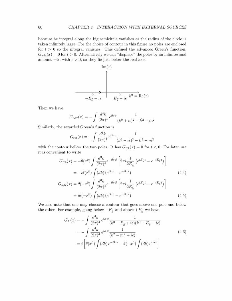
60 CHAPTER 4. INTERACTION WITH EXTERNAL SOURCES
because he integral along the big semicircle vanishes as the radius of the circle istaken infinitely large. For the choice of contour in this figure no poles are enclosedfor t > 0 so the integral vanishes. This defined the advanced Green’s function,Gadv(x) = 0 for t > 0. Alternatively we can “displace” the poles by an infinitesimalamount −iε, with ε > 0, so they lie just below the real axis,
k0 = Re(z)
Im(z)
×E~k − iε
×−E~k − iε
Then we have
Gadv(x) = −∫
d4k
(2π)4eik·x
1
(k0 + iε)2 − ~k 2 −m2
Similarly, the retarded Green’s function is
Gret(x) = −∫
d4k
(2π)4eik·x
1
(k0 − iε)2 − ~k 2 −m2
with the contour bellow the two poles. It has Gret(x) = 0 for t < 0. For later useit is convenient to write
Gret(x) = −θ(x0)
∫d3k
(2π)4e−i
~k ·~x[2πi
1
2E~k
(eiE~k t − e−iE~k t
)]= −iθ(x0)
∫(dk) (eik·x − e−ik·x) (4.4)
Gadv(x) = θ(−x0)
∫d3k
(2π)4e−i
~k ·~x[2πi
1
2E~k
(eiE~k t − e−iE~k t
)]= iθ(−x0)
∫(dk) (eik·x − e−ik·x) (4.5)
We also note that one may choose a contour that goes above one pole and belowthe other. For example, going below −E~k and above +E~k we have
GF (x) = −∫
d4k
(2π)4eik·x
1
(k0 − E~k + iε)(k0 + E~k − iε)
= −∫
d4k
(2π)4eik·x
1
(k2 −m2 + iε)
= i
[θ(x0)
∫(dk) e−ik·x + θ(−x0)
∫(dk) eik·x
] (4.6)
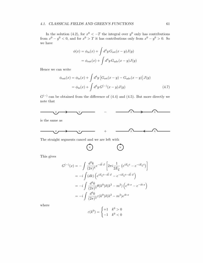
4.1. CLASSICAL FIELDS AND GREEN’S FUNCTIONS 61
In the solution (4.2), for x0 < −T the integral over y0 only has contributionsfrom x0 − y0 < 0, and for x0 > T it has contributions only from x0 − y0 > 0. Sowe have
φ(x) = φin(x) +
∫d4y Gret(x− y)J(y)
= φout(x) +
∫d4y Gadv(x− y)J(y)
Hence we can write
φout(x) = φin(x) +
∫d4y
[Gret(x− y)−Gadv(x− y)
]J(y)
= φin(x) +
∫d4y G(−)(x− y)J(y) (4.7)
G(−) can be obtained from the difference of (4.4) and (4.5). But more directly wenote that
×× − ××
is the same as
×× + ××
The straight segments cancel and we are left with
××
This gives
G(−)(x) = −∫
d3k
(2π)4e−i
~k ·~x[2πi
1
2E~k
(eiE~k t − e−iE~k t
)]= −i
∫(dk)
(eiE~k t−i
~k ·~x − e−iE~k t−i~k ·~x)
= −i∫
d4k
(2π)3θ(k0)δ(k2 −m2)
(eik·x − e−ik·x
)= −i
∫d4k
(2π)3ε(k0)δ(k2 −m2)eik·x
where
ε(k0) =
+1 k0 > 0
−1 k0 < 0

62 CHAPTER 4. INTERACTION WITH EXTERNAL SOURCES
You may have noticed that this looks a lot like the function ∆+(x) = [φ(+)(x), φ(−)(0)].In fact, computing the commutator of free fields at arbitrary times,
[φ(x), φ(y)] =
∫(dk)(dk′)[α~k
e−ik·x + α†~keik·x, α~k ′
e−ik′·y + α†~k ′
eik′·y]
=
∫(dk)
[eik·(y−x) − e−ik·(y−x)
]= iG(−)(y − x) = −iG(−)(x− y)
4.2 Quantum Fields
We now consider equation (4.1) for the KG field with a source in the case thatthe field is an operator on the Hilbert space F . The source J(x) is a a c-number,a classical source, and still take it to be localized in space-time. Suppose thesystem is in some state initially, well before the source is turned on. Let’s take thevacuum state for definiteness, although any other state would be just as good. Asthe system evolves, the source is turned on and then off, and we end up with thesystem in some final state. Now, in the classical case if we start from nothing andturn the source on and then off radiation is produced, emitted out from the regionof the localized source. In the quantum system we therefore expect we will get afinal state with any number of particles emitted from the localized source region.
Then φ(x) = φin(x) is the statement that for t < −T φ is the same operatoras a solution to the free KG equation. Likewise for φ = φout for t > T . Doesthis mean φout = φin? Surely not, it is not true in the classical case. Sinceφ satisfies the equal time commutation relations, i[∂tφ(x), φ(y)] = δ(3)(~x − ~y ),etc, so do φout and φin. Since the latter solve the free KG equation, they haveexpansions in creation and annihilation operators, and the same Hilbert space.More precisely, we can construct a Fock space Fin out of α†in, and a space Fout out
of α†out. These spaces are just Hilbert spaces of the free KG equation, and thereforethey are isomorphic, Fin ≈ Fout ≈ FKG. So there is some linear, invertible operatorS : FKG → FKG, so that |ψ〉out = S−1|ψ〉in. Since the states are normalized, Smust preserve normalization, so S is unitary, S†S = SS† = 1. The operator S iscalled the S-matrix.
Let’s understand the meaning of |ψ〉out = S†|ψ〉in. The state of the systeminitially (far past) is |ψ〉in. It evolves into a state |ψ〉out = S†|ψ〉in at late times,well after the source is turned off. We can expand it in a basis of the Fock space,the states |~k 1, . . . ,~k n〉 for n = 0, 1, 2, . . . In particular, if the initial state is thevacuum, then the expansion of S†|0〉 in the Fock space basis tells us the probabilityamplitude for emitting any number of particles. More generally
out〈χ|ψ〉in = in〈χ|S|ψ〉in

4.2. QUANTUM FIELDS 63
is the probability amplitude for starting in the state |ψ〉 and ending in the state|χ〉. Note that the left hand side is not to be taken literally as an inner productin the same Hilbert space of free particles (else it would vanish except when theinitial and final states are physically identical, i.e., when nothing happens).
Now, S†φin(x)S is an operator acting on out states that satisfies the KG equa-tion. Similarly, if πin(x) = ∂tφin(x), S†πin(x)S acts on out states. Moreover, thecommutator [S†φin(x)S, S†πin(y)S = S†[φin(x), πin(y)]S = [φin(x), πin(y)] since thecommutator is a c-number and S†S = 1, and similarly for the other commutatorsof S†φin(x)S and S†πin(x)S. This means that up to a canonical transformation,
φout(x) = S†φin(x)S .
Since we are free to choose the out fields in the class of canonical equivalent fields,we take the above relation to be our choice.
There is a simple way to determine S. We will present this now, but themethod works only for the case of an external source and cannot be generalizedto the case of interacting fields. So after presenting this method we will present amore powerful technique that can be generalized. From Eq. (4.7) we have
S†φin(x)S = φin(x) +
∫d4y G(−)(x− y)J(y)
= φin(x) + i
∫d4y [φin(x), φin(y)J(y)] .
Recall
eABe−A = B + [A,B] + 12 [A, [A,B]] + · · ·
= B + [A,B] if [A, [A,B]] = 0.
It follows that
S = exp
[i
∫d4y φin(y)J(y)
](4.8)
It is convenient to normal-order S. Since [φ(+)(x), φ(−)(y)] is a c-number we canuse
eAeB = eA+B+ 12
[A,B]
which is valid provided [A,B] commutes with bothA andB. So using i∫d4xφ(−)(x)J(x)
and i∫d4xφ(+)(x)J(x) for A and B,
S = ei∫d4xφ(−)(x)J(x)ei
∫d4xφ(+)(x)J(x)e
12
∫d4x d4y [φ(−)(x),φ(+)(y)]J(x)J(y)

64 CHAPTER 4. INTERACTION WITH EXTERNAL SOURCES
From (2.10),
∆+(x2 − x1) ≡ [φ(+)(x1), φ(−)(x2)]
=
∫(dk) e−ik·(x2−x1)
=
∫d4k
(2π)4θ(k0)δ(k2 −m2)e−ik·(x2−x1)
and introducing the Fourier transform of the source,
J(x) =
∫d4k
(2π)4eik·xJ(k)
we have∫d4x d4y [φ
(−)in (x), φ
(+)in (y)]J(x)J(y)
= −∫ 3∏
i=1
d4ki(2π)4
θ(k01)δ(k2
1 −m2)J(k2)J(k3)
∫d4x
∫d4y eik2·xeik3·yeik1·(y−x)
= −∫
d4k
(2π)4θ(k0)δ(k2 −m2)J(k)J(−k) = −
∫(dk)|J(k)|2 ,
where we have used J∗(x) = J(x) ⇒ J(−k) = J∗(k), and it is understood thatk0 = E~k . Hence,
S = ei∫d4xφ(−)(x)J(x)ei
∫d4xφ(+)(x)J(x)e−
12
∫(dk)|J(k)|2 .
As an example of an application, we can compute the probability of finding par-ticles in the final state if we start form no particles initially (emission probability).Start from probability of persistence of the vacuum,
|out〈0|0〉in|2 = |in〈0|S|0〉in|2 = exp
(−∫
(dk)|J(k)|2).
Next compute the probability that one particle is produced with momentum ~k :
|out〈~k |0〉in|2 = |in〈~k |S|0〉in|2 = |in〈0|α~kS|0〉in|2 .
where “in” in α~k is implicit. To proceed we use
[α~k , φ(−)(x)] =
∫(dk′)[α~k , α
†~k ′
]eik′·x = eik·x (with k0 = E~k )

4.2. QUANTUM FIELDS 65
so that
e−i∫φ(−)Jα~k e
i∫φ(−)J = α~k−i
∫[φ(−), α~k ]J = α~k+i
∫d4xeik·xJ(x) = α~k+iJ(−k) .
Hence
|out〈~k |0〉in|2 = |J(k)|2 exp
(−∫
(dk)|J(k)|2).
4.2.1 Phase Space
Suppose we want to find the probability of finding a single particle as t → ∞regardless of its momentum, that is, in any state. We need to sum over all finalstates consisting of a single particle, once each. Since we have a continuum of stateswe have to integrate over all ~k with some measure,
∫dµ(~k ). Clearly dµ(~k ) must
involve d3k, possibly weighted by a function f(~k ). Presumably this function isrotationally invariant, f = f(|~k |). But we suspect also dµ(~k ) is Lorentz invariant,so dµ(~k ) ∝ (dk), that is, it equals the invariant measure up to a constant. Let’sfigure this out by counting. Note that how we normalize states matters.
First we determine this via a shortcut, and later we repeat the calculation viaa more physical approach (and obtain, of course the same result). We want
∑n
|out〈n|0〉in|2 =∑n
in〈0|n〉out out〈n|0〉in = out〈0|
(∑n
|n〉out out〈n|out
)|0〉in ,
where the sum is restricted over some states. The operator∑n
|n〉out out〈n|
is a projection operator onto the space of “some states,” the ones we want to sumin the final state. We have already discussed this projection operator for the caseof one particle states when |~k 〉 is relativistically normalized. It is∫
(dk)|~k 〉〈~k | .
So we have
1-particle emission probability =
∫(dk)|J(k)|2 exp
(−∫
(dk)|J(k)|2).
Now we repeat the calculation by counting states. It is easier to count discretesets of states. We can do so by placing the system in a box of volume LxLyLz.
Take, say, periodic boundary conditions. Then instead of∫
(dk)(α~k ei~k ·~x +h.c.), we

66 CHAPTER 4. INTERACTION WITH EXTERNAL SOURCES
have a Fourier sum,∑
~k(a~k e
i~k ·~x + h.c.). Here a~k are creation operators with somenormalization we will have to sort out. For periodic boundary conditions we musthave kxLx = 2πnx, kyLy = 2πny, kzLz = 2πnz, with ni integers. We label the one
particle states by these, |~n〉 = a†~k|0〉, where ~k = 2π
(nxLx,nyLy, nzLz
). The probability
of finding |ψ〉 in state |~n〉 is |〈~n |ψ〉|2 if both |ψ〉 and |~n〉 are normalized to unity.
(Note that this means [a~k , a†~k ′
] = δnxn′xδnyn′yδnzn′z). The probability of finding |ψ〉in a 1-particle state is then
∑~n |〈~n |ψ〉|2.
Let’s be more specific. What is the probability of finding |ψ〉 in a 1-particlestate with momentum in a box (kx, kx + ∆kx) × (ky, ky + ∆ky) × (kz, kz + ∆kz)?
There are ∆nx∆ny∆nz =LxLyLz
(2π)3∆kx∆ky∆kz state in the box. For large volume
the spacing between values of ~k becomes small, so in the limit of large volume∆kx → dkx, etc, and the number of particles in the momentum box is
LxLyLz(2π)3
∆kx∆ky∆kz → Vd3k
(2π)3
where V = LxLyLz is the volume fo the box. As we switch from discrete to con-tinuum labels for our states we must be careful with their normalization condition.Since on the space of 1-particle states we have∑
~n
|~n〉〈~n | = 1 ⇒∑~n
|~n〉〈~n |~n ′〉 = |~n ′〉
then in the limit, denoting by |~k 〉 the continuum normalized states,
∑~n
V∆3k
(2π)3|~n〉〈~n |~n ′〉 = |~n ′〉 →
∫d3k|~k 〉〈~k |~k ′〉 = |~k ′〉
⇒ V
(2π)3δnxn′xδnyn′yδnzn′z → δ(3)(~k − ~k ′) .
Putting these elements together, the probability of finding |ψ〉 in a 1-particle stateis ∑
~n
|〈~n |ψ〉|2 →∫d3k|〈~k |ψ〉|2 .
Finally, if we want to change the normalization of states so that 〈~k ′|~k 〉 = N~k δ(3)(~k−
~k ′) then the probability of finding |ψ〉 in a 1-particle state is∫d3k
N~k|〈~k |ψ〉|2 .

4.2. QUANTUM FIELDS 67
For relativistic normalization of states, N~k = (2π)32E~k and the probability is∫(dk)|〈~k |ψ〉|2 .
This is precisely our earlier result. Denoting the emission probability for n particlesin the presence of a localized source J(x) by pn, we have
p0 = e−ξ, p1 = ξe−xi, where ξ =
∫(dk)|J(~k )|2 . (4.9)
4.2.2 Poisson
We can now go on to compute pn for arbitrary n. Start with n = 2, that is, emissionof two particles.
e−i∫φ(−)Jα~kα~k ′e
i∫φ(−)J = e−i
∫φ(−)Jα~k e
i∫φ(−)Je−i
∫φ(−)Jα~k ′e
i∫φ(−)J
= (α~k + iJ(−k))(α~k ′ + iJ(−k′)) (4.10)
so that
out〈~k~k ′|0〉in = −J(−k)J(−k′)e−12ξ .
To get the emission probability we must sum over all distinguishable 2-particlestates. Since |~k~k ′〉 = |~k ′~k 〉 we must not double count. When we integrate over abox in momentum space, we count twice the state |~k~k ′〉 if we sum over k1 and k2
with values k1 = k, k2 = k′ and k1 = k′, k2 = k:
kx
k′x
= 12 ×
kx
k′x
Hence
p2 = 12ξ
2e−ξ .
The generalization is straightforward:
pn =1
n!ξn exp(−ξ) .
This is a Poisson distribution! Note that∑
n pn = 1, that is, there is certainty offinding anything (that is, either no or some particles). The mean of the distributionis ξ =
∫(dk)|J(~k )|2.
68 CHAPTER 4. INTERACTION WITH EXTERNAL SOURCES
4.3 Evolution Operator
We now introduce a more general formalism to derive the same results, but thatwill be more useful when we consider interacting quantum fields. We want toconstruct an operator U(t) that gives the connection between the field φ and the“in” field φin:
φ(~x, t) = U−1(t)φin(~x, t)U(t) . (4.11)
Since we are assuming φ→ φin as t→ −∞, we must have
U(t)→ 1 as t→ −∞ . (4.12)
The S matrix is then
S = limt→∞
U(t) .
The time evolution of φ and φin are given by
∂φ
∂t(~x, t) = i[H(t), φ(~x, t)]
∂φin
∂t(~x, t) = i[H0in(t), φin(~x, t)] (4.13)
Here H = H0 +H ′, where H0 is the free Hamiltonian and H ′ describes interactions.In the present case,
H0 =
∫d3x
[12π
2 + 12(~∇φ)2 + 1
2m2φ2]
H ′(t) =
∫d3xJ(~x, t)φ(~x, t) .
Also the subscript “in” means the argument has “in” fields. So H = H(φ, π, J)with H0 = H0(φ, π) while H0in = H0in(φin, πin). From Eq. (4.11) we have
U−1(t)H(φ(t), π(t), J(t))U(t)
= H(U−1(t)φ(t)U(t), U−1(t)π(t)U(t), U−1(t)J(t)U(t))
= H(φin(t), πin(t), J(t)) (4.14)
and
∂φin
∂t(~x, t) =
∂
∂t
[Uφ(~x, t)U−1(t)
]=dU
dtφU−1 + Uφ
dU−1
dt+ Ui[H(t), φ(~x, t)]U−1
=dU
dtU−1φin − φin
dU
dtU−1 + i[Hin(t), φin(~x, t)]
= i[−idUdtU−1 +Hin(t), φin(~x, t)]

4.3. EVOLUTION OPERATOR 69
Comparing with Eq. (4.13) this is the commutator with H0in so we must have
−idUdtU−1 +Hin(t) = H0in(t)
ordU
dt= −i(Hin −H0in)U = −iH ′inU (4.15)
The solution to this equation with the boundary condition (4.12) gives the S matrix,S = U(∞). Note that the equation contains only “in” fields, which we know howto handle.
We can solve (4.15) by iteration. Integrating (4.15) form −∞ to t we have
U(t)− 1 = −i∫ t
−∞dt′H ′in(t′)U(t′) .
Now use this again, repeatedly,
U(t) = 1− i∫ t
−∞dt′H ′in(t′)
[1− i
∫ t′
−∞dt′′H ′in(t′′)U(t′′)
]
= 1− i∫ t
−∞dt1H
′in(t1) + (−i)2
∫ t
−∞dt1
∫ t1
−∞dt2H
′in(t1)H ′in(t2)U(t2)
= · · · = 1 +
∞∑n=1
(−i)n∫ t
−∞dt1
∫ t1
−∞dt2 · · ·
∫ tn−1
−∞dtnH
′in(t1)H ′in(t2) · · ·H ′in(tn) .
Note that the product H ′in(t1)H ′in(t2) · · ·H ′in(tn) is time-ordered, that is, the Hamil-tonians appear ordered by t ≥ t1 ≥ t2 · · · ≥ tn. This is the main result of thissection.
We can write the result more compactly. Note that∫ t
−∞dt1
∫ t1
−∞dt2H
′in(t1)H ′in(t2) =
∫ t
−∞dt2
∫ t2
−∞dt1H
′in(t2)H ′in(t1)
The two integrals together cover the region −∞ < t1 ≤ t, −∞ < t2 ≤ t of thet1 vs t2 plane, as can be seen from the followin figures in which the shaded regionscorrespond to the region of integration of the first and second integrals, respectively:
t1
t2
t
t
t1
t2
t
t

70 CHAPTER 4. INTERACTION WITH EXTERNAL SOURCES
For any two time dependent operators, A(t) and B(t), we define the time-orderedproduct
T (A(t1)B(t2)) = θ(t1−t2)A(t1)B(t2)+θ(t2−t1)B(t2)A(t1) =
A(t1)B(t2) t1 > t2
B(t2)A(t1) t2 > t1
and similarly when there are more than two operators in the product. Then∫ t
−∞dt1
∫ t1
−∞dt2H
′in(t1)H ′in(t2) =
1
2
∫ t
−∞dt1
∫ t
−∞dt2T
(H ′in(t1)H ′in(t2)
).
For the term with n integrals there are n! orderings of t1, . . . , tn so we obtain
U(t) = 1 +∞∑n=1
(−i)n
n!
∫ t
−∞dt
∫ t
−∞dt2 · · ·
∫ t
−∞dtn T (H ′in(t1)H ′in(t2) · · ·H ′in(tn)) .
(4.16)or, comparing with ez =
∑∞n=0
1n!z
n we write
U(t) = T
[exp
(−i∫ t
−∞dt′H ′in(t′)
)].
You should keep in mind that the meaning of this expression is the explicit expan-sion in (4.16). Finally, taking t→∞,
S = T
[exp
(−i∫ ∞−∞
dtH ′in(t)
)]= T
[exp
(−i∫d4xH′in
)]or, using L′ = −H′,
S = T
[exp
(i
∫d4xL′in
)].
Let’s use this general result for the specific example we have been discussing,and compare with previous results. Use L′in = J(x)φin(x). Then
S = T
[exp
(i
∫d4xJ(x)φin(x)
)].
But we had obtained
S = e−12ξ :exp
(i
∫d4xJ(x)φin(x)
): (4.17)
with ξ = 12
∫(dk)|J(k)|2, as in (4.9). Are these two expression for S the same? To
show they are we need some additional machinery, some relation between T-orderedand normal-ordered products.

4.4. WICK’S THEOREM 71
4.4 Wick’s Theorem
In order to answer the question, what is the difference between T-ordered andnormal-ordered products, we consider
T (φ(x1)φ(x2))− :φ(x1)φ(x2):
Here and below φ stands for an “in” field, that is, a free field satisfying the KGequation. For notational conciseness we write φi for φ(x1, etc. Letting φ = φ(+) +φ(−) and taking x0
1 > x02 the difference is
(φ(+)1 +φ
(−)1 )(φ
(+)2 +φ
(−)2 )−(φ
(+)1 φ
(+)2 +φ
(−)1 φ
(+)2 +φ
(−)2 φ
(+)1 +φ
(−)1 +φ
(−)2 ) = [φ
(+)1 , φ
(−)2 ]
This is a c-number (equals ∆+(x2 − x1)). Taling the expectation value in thevacuum we obtain, restoring full notation momentarily,
T (φ(x1)φ(x2)) = :φ(x1)φ(x2): +〈0|T (φ(x1)φ(x2))|0〉 .
Clearly this holds for the more general case of several fields,
T (φn(x1)φm(x2)) =: :φn(x1)φm(x2): +〈0|T (φn(x1)φm(x2))|0〉 .
Consider next the case of three fields, T (φ1φ2φ3). Without loss of generalitytake x0
1 ≥ x02 ≥ x0
3:
T (φ1φ2φ3) = φ1φ2φ3 = φ1(:φ2φ3: +〈0|T (φ2φ3)|0〉)
Now, φ1 :φ2φ3: = (φ(+)1 + φ
(−)1 ) :φ2φ3:. We need to move φ
(+)1 to the right of all of
the φ(−) operators:
φ(+)1 :φ2φ3: = :φ2φ3:φ
(+)1 + [φ
(+)1 , φ
(−)2 ] :φ3: +[φ
(+)1 , φ
(−)3 ] :φ2:
where we have used the fact that [φ(+)1 , φ
(−)n ] is a c-number. In fact, it equals
〈0|T (φ1φn)|0〉. So we have
T (φ1φ2φ3) = :φ1φ2φ3: + :φ1:〈0|T (φ2φ3)|0〉+ :φ2:〈0|T (φ1φ3)|0〉+ :φ3:〈0|T (φ1φ2)|0〉 .
Of course, :φ: = φ, but the notation will more easily generalize below.More notation, rewrite the above as
T (φ1φ2φ3) = :φ1φ2φ3: + :φ1φ2φ3: + :φ1φ2φ3: + :φ1φ2φ3: .
where
φnφm = 〈0|T (φnφm)|0〉

72 CHAPTER 4. INTERACTION WITH EXTERNAL SOURCES
is called a contraction.
Wick’s theorem states that
T (φ1 · · ·φn) = :φ1 · · ·φn: +∑pairs(i,j)
:φ1 · · ·φi · · ·φj · · ·φn:
+∑
2-pairs(i,j),(k,l)
:φ1 · · ·φi · · ·φj · · ·φk · · ·φl · · ·φn: + · · ·
+
:φ1φ2φ3φ4 · · ·φn−1φn: +all pairings n = even
:φ1φ2φ3φ4 · · ·φn−2φn−1φn: +all pairings n = odd(4.18)
In words, the right hand side is the sum over all possible contractions in the normalordered product :φ1 · · ·φn: (including the term with no contractions). The proof isby induction. We have already demonstrated this for n = 2, 3. Let W (φ1, . . . , φn)stand for the right hand side of (4.18), and assume the theorem is valid for n− 1fields. Then assuming x0
1 ≥ x02 ≥ · · · ≥ x0
n,
T (φ1 · · ·φn) = φ1T (φ1 · · ·φn)
= φ1W (φ2, . . . , φn)
= (φ(+)1 + φ
(−)1 )W (φ2, . . . , φn)
= φ(−)1 W (φ2, . . . , φn) +W (φ2, . . . , φn)φ
(+)1 + [φ
(+)1 ,W (φ2, . . . , φn)]
The first two terms are normal ordered and contain all contractions that do notinvolve φ1. The last term involves the contractions of φ1 with every field in everyterm in W (φ2, . . . , φn), therefore all possible contractions. Hence the right handside contains all possible contractions, which is W (φ1, . . . , φn).
4.4.1 Combinatorics
Let’s go back to our computation of S. We’d like to use Wick’s theorem to re-late T [exp(i
∫d4xφin(x)J(x))] to :exp(i
∫d4xφin(x)J(x)):, and for this we need
a little combinatorics. To make the notation more compact we will continuedropping the “in” label on the “in” fields for the rest of this section. Now,T [exp(i
∫d4xφin(x)J(x))] is a sum of terms of the form
in
n!
∫ n∏i=1
d4xi J1 · · · JnT (φ1 · · ·φn) =in
n!
∫ n∏i=1
d4xi J1 · · · JnW (φ1, . . . , φn) (4.19)
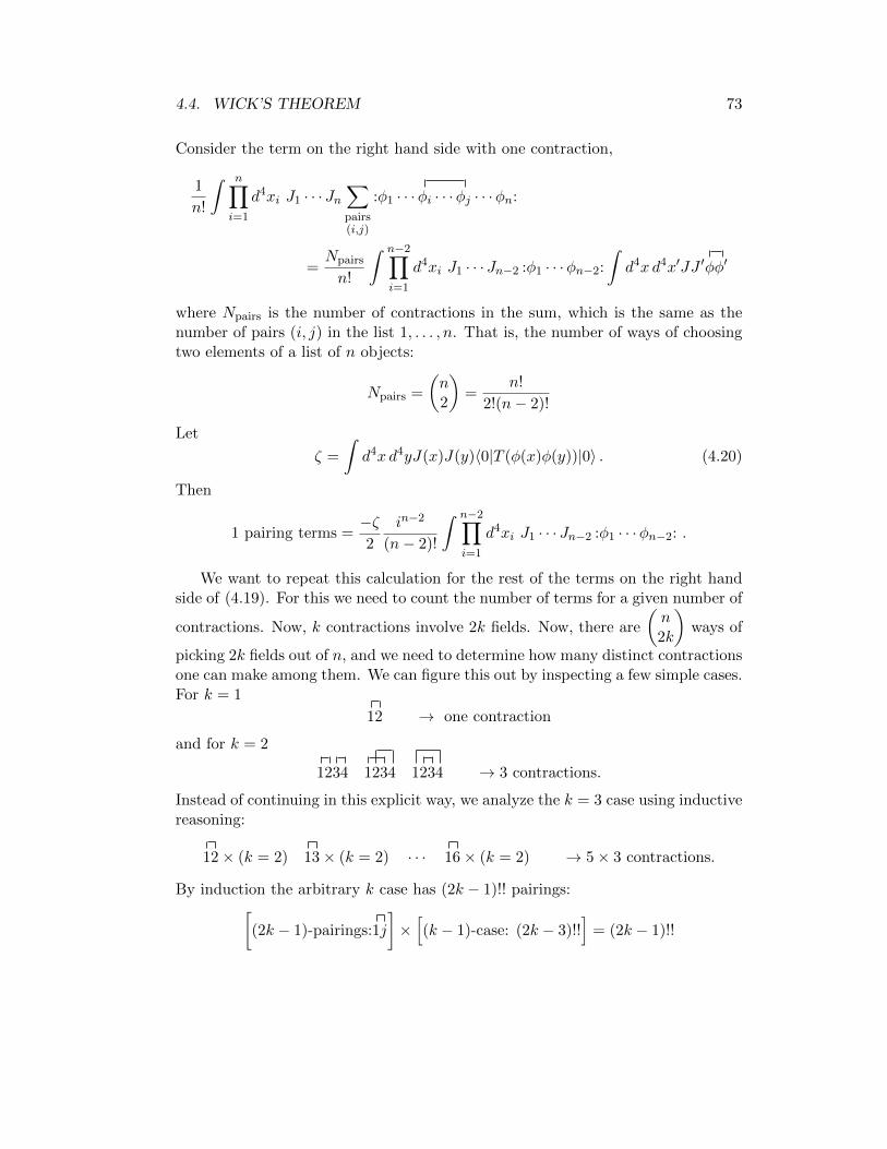
4.4. WICK’S THEOREM 73
Consider the term on the right hand side with one contraction,
1
n!
∫ n∏i=1
d4xi J1 · · · Jn∑pairs(i,j)
:φ1 · · ·φi · · ·φj · · ·φn:
=Npairs
n!
∫ n−2∏i=1
d4xi J1 · · · Jn−2 :φ1 · · ·φn−2:
∫d4x d4x′JJ ′φφ′
where Npairs is the number of contractions in the sum, which is the same as thenumber of pairs (i, j) in the list 1, . . . , n. That is, the number of ways of choosingtwo elements of a list of n objects:
Npairs =
(n2
)=
n!
2!(n− 2)!
Let
ζ =
∫d4x d4yJ(x)J(y)〈0|T (φ(x)φ(y))|0〉 . (4.20)
Then
1 pairing terms =−ζ2
in−2
(n− 2)!
∫ n−2∏i=1
d4xi J1 · · · Jn−2 :φ1 · · ·φn−2: .
We want to repeat this calculation for the rest of the terms on the right handside of (4.19). For this we need to count the number of terms for a given number of
contractions. Now, k contractions involve 2k fields. Now, there are
(n2k
)ways of
picking 2k fields out of n, and we need to determine how many distinct contractionsone can make among them. We can figure this out by inspecting a few simple cases.For k = 1
12 → one contraction
and for k = 2
1234 1234 1234 → 3 contractions.
Instead of continuing in this explicit way, we analyze the k = 3 case using inductivereasoning:
12× (k = 2) 13× (k = 2) · · · 16× (k = 2) → 5× 3 contractions.
By induction the arbitrary k case has (2k − 1)!! pairings:[(2k − 1)-pairings:1j
]×[(k − 1)-case: (2k − 3)!!
]= (2k − 1)!!

74 CHAPTER 4. INTERACTION WITH EXTERNAL SOURCES
So the terms with k contractions give
1
n!
n!
(n− 2k)!(2k)!(2k − 1)!!︸ ︷︷ ︸
1
(n− 2k)!
1
2kk!
in−2k
∫ n−2k∏i=1
d4xiJ1 · · · Jn−2k :φ1 · · ·φn−2k:
(i2∫d4x d4x′ JJ ′φφ′
)k︸ ︷︷ ︸
(−1)kζk
=(−ζ/2)k
k!
im
m!
∫ m∏i=1
d4xi J1 · · · Jm :φ1 · · ·φm: with m = n− 2k.
Aha! We recognize this as a term in an exponential expansion. Consideringall the terms in he expansion of T [exp(i
∫d4xφin(x)J(x))], the coefficient of
im
m!
∫ ∏mi=1 d
4xi J1 · · · Jm :φ1 · · ·φm: (fixed m) is∑∞
k=01k!(−ζ/2)k = exp(−1
2ζ), andis independent of m, so it factors out. We are left with
e−ζ/2∞∑m=0
im
m!
∫ m∏i=1
d4xi J1 · · · Jm :φ1 · · ·φm: = e−ζ/2 :exp
(i
∫d4xJ(x)φ(x)
):
That is
S = T
[exp
(i
∫d4xφin(x)J(x)
)]= e−ζ/2 :exp
(i
∫d4xJ(x)φ(x)
):
This will equal our previous expression for S in (4.17) if ζ = ξ. To answer this weneed to know more about the T-ordered product in the definition of ζ in (4.20).
4.5 Scalar Field Propagator
Let∆F (x, y) ≡ 〈0|T (φ(x)φ(y))|0〉
where φ(x) is a real, scalar, free field satisfying the Klein-Gordon equation. This isthe quantity we need for the computation fo ζ, but it is also important for severalother reasons, so we spend some time investigating it.
First of all, i∆F (x, y) is a Green’s function for the Klein-Gordon equation; see(4.3). To verify this claim compute directly. Taking ∂µ to be the derivative withrespect to xµ keeping yµ fixed and using (∂2 +m2)φ(x) = 0 we have
(∂2 +m2)∆F (x, y) = (∂2 +m2)[θ(x0 − y0)〈0|φ(x)φ(y)|0〉+ θ(y0 − x0)〈0|φ(y)φ(x)|0〉
]=
∂2
∂x02θ(x0 − y0)〈0|φ(x)φ(y)|0〉+
∂2
∂x02θ(y0 − x0)〈0|φ(y)φ(x)|0〉
+ 2∂
∂x0θ(x0 − y0)〈0|∂φ(x)
∂x0φ(y)|0〉+ 2
∂
∂x0θ(y0 − x0)〈0|φ(y)
∂φ(x)
∂x0|0〉

4.5. SCALAR FIELD PROPAGATOR 75
Now using dθ(x)/dx = δ(x) and ∂0φ(x) = π(x) the last line above is
2δ(x0 − y0)〈0|[π(x), φ(y)]|0〉 = −2iδ(4)(x− y)
The line above that gives
∂
∂x0δ(x0 − y0)〈0|[φ(x), φ(y)]|0〉 = −δ(x0 − y0)〈0|[π(x), φ(y)]|0〉 = iδ(4)(x− y)
Combining these we have
(∂2 +m2)∆F (x, y) = −iδ(4)(x− y)
As we saw in Sec. 4.1 Green functions are not unique, since one can always add solu-tions to the homogenous Klein-Gordon equation to obtain a new Green’s function.We must have
i∆F (x, y) = −i∫
d4k
(2π)4eik·(x−y) 1
k2 −m2
with some prescription for the contour of integration. Note that ∆F (x, y) = ∆F (x−y) depends only on the difference x − y, which is as expected from homogeneitypof space-time.
Recall that [φ(+)(x), φ(−)(y)] = 〈0|Tφ(x)φ(y)|0〉 for x0 > y0. More generally
〈0|Tφ(x)φ(y)|0〉 = θ(x0 − y0)[φ(+)(x), φ(−)(y)] + θ(y0 − x0)[φ(+)(y), φ(−)(x)]
Recall also that
[φ(+)(x), φ(−)(y)] =
∫(dk)e−iE~k (x0−y0)+i~k ·(~x−~y )
Without loss of generality and to simplify notation we set yµ = 0. We have
〈0|Tφ(x)φ(0)|0〉 = θ(x0)
∫(dk)e−iE~k x
0+i~k ·~x + θ(−x0)
∫(dk)eiE~k x
0−i~k ·~x
Comparing with Eq. (4.6) we see this is precisely −iGF (x), which was obtained bytaking a contour that goes below −E~k and above E~k ,
k0 = Re(z)
Im(z)
×E~k − iε
×−E~k + iε

76 CHAPTER 4. INTERACTION WITH EXTERNAL SOURCES
So we have
〈0|Tφ(x)φ(y)|0〉 =
∫d4k
(2π)4e−ik·(x−y) i
k2 −m2 + iε(4.21)
This will be of much use later. We will refer to this as the two-point function ofthe KG field, and the Fourier transform, 1/(k2 −m2 + iε), as the KG propagator.
We can finally return to the question of relating ζ to ξ:
ζ =
∫d4x d4y J(x)J(y) 〈0|Tφ(x)φ(y)|0〉
=
∫d4x d4y
∫d4k1
(2π)4
d4k2
(2π)4eik1·xeik2·yJ(k1)J(k2)
∫d4p
(2π)4e−ip·(x−y) i
p2 −m2 + iε
=
∫d4p
(2π)4J(p)J(−p) i
p2 −m2 + iε
Perform the integral over p0, assuming J(p)J(−p) = |J(p)|2 vanishes as |p0| → ∞,which is justified by our assumption that the source is localized in space-time.Closing the contour on the upper half of the complex p0 plane we pick the pole at−E~k so that
ζ = 2πi
∫d3p
(2π)4|J(p)|2 i
−2E~k=
∫(dk)|J(p)|2 = ξ .

Chapter 5
Elementary Processes
We want to extend the previous discussion to the case where fields interact amongthemselves, rather than with an external source. The aim is to give an expressionfor the S-matrix in terms of “in” fields, as before. We will see that uit is con-venient to express the matrix elements of S in terms of Green’s functions, thatis, vacuum expectation values of time-ordered products of elementary fields, as in〈0|Tφ(x1) · · ·φ(xn)|0〉.
As before the S matrix connects |in〉 states to |out〉 states, |out〉 = S−1|in〉, andcorrespondingly φin fields to φout fields. But we can no longer say that φ(x) →φin(x) as t → −∞ (nor φ(x) → φout(x) as t → +∞) with φin,out(x) free fields (afree field is one without interactions, e.g., it satisfies the KG equation).
Before we explain that in more detail let us better understand the role of |in〉states (and φin fields). In a collision process we start with particles that are wildlyseparated, so interactions between them can be initially neglected. As particlesapproach each other the interactions can no longer be neglected, they “turn on.”So one could think of the situation by replacing H ′ (the interaction part of theHamiltonian) by f(t)H ′, where f(t) is a smooth function that turns on slowly(adiabatically), then stays on for some long period over which the collision takesplace, say, f(t) = 1 for −T < t < T , and then turns off slowly again, f(t) = 0|t| > T0 and f(t) smoothly decreasing (increasing) in T < t < T0 (−T0 < t < −T ):
t
f(t)
T−T T0−T0
We want both T and T0 to be arbitrarily large, and we want T0 T in the
77

78 CHAPTER 5. ELEMENTARY PROCESSES
process to avoid sudden changes that can introduce extraneous effects, e.g., pairproduction.
We will use this model, but it is not quite general enough. The reason isthat if the interaction is turned off we may not be able to describe |in〉 and |out〉states of interest, namely, bound states that arise because of the interaction. Forexample, we may want to study collisions of an electron with an H atom due toelectromagnetic interactions. But it is the electromagnetic interactions that bindsa p and an e into an H atom. More poignant is the case of collisions of protonsby the strong interactions when it is these interactions that keeps quarks bound inprotons. The idea of collision theory is that oen can set up a muck theory of freeparticles that happen to have the same mass (and other quantum numbers, e.g.,spin) as the bound states. These are the |in〉 and |out〉 states. For very early (orlate) times these states describe the evolution of the particles that later (earlier)participate in the collision. And the S-matrix uses information in the interactingtheory to connect the pre- and post-collision states. For theories without boundstates we can use the simpler approximation of turning on and off the interactionvia f(t)H ′. Remarkably the expression for the S-matrix obtained via this simplifiedtreatment is the same as in a more complete and rigorous analysis that does notemploy it.
If we adiabatically turn on and off the interactions then we can use our previousapproach:
φ(x) = φin(x) +
∫d4y Gret(x− y)J(y) (5.1)
But now
(∂2 +m2)φ =L′
∂φ
(e.g., if L′ = gφ3 +λφ4 then L′
∂φ = 3gφ2 + 4λφ4). So for J(x) use f(t) L′
∂φ . Note thatin the absence of f(t) this would not work, the “source” would not be localized intime. Now, we had two ways of obtaining the S-matrix from this. One was
S†φin(x)S = φin(x) +
∫d4y [φin(x), φin(y)]J(y) .
But now J(y) depends on φ(x) so it does not commute with φin(x). This makes itharder to solve for S using this method.
The second method used φ = U †(t)φin(x)U(t) and constructed U(t) in termsof H′. This will work. The result was, and still is,
S = T
[exp
(i
∫d4xL′in
)]which we can use, but now with, say, L′in = gφ3
in + λφ4in.
However, the above discussion has to be modified, as we will see shortly, becausein general one cannot take φ(x)→ φin(x) as t→ −∞.

5.1. KALLEN-LEHMANN SPECTRAL REPRESENTATION 79
5.1 Kallen-Lehmann Spectral Representation
Here we will see that we cannot take φ(x) → φin(x) as t → −∞. We study[φ(x), φ(y)] and compare with [φin(x), φin(y)]. In particular,
〈0|[φ(x), φ(y)]|0〉 =∑∫
n(〈0|φ(x)|n〉〈n|φ(y)|0〉 − x↔ y)
Now
〈0|φ(x)|n〉 = 〈0|eiP ·xφ(0)e−iP ·x|n〉 = e−ipn·x〈0|φ(0)|n〉
where Pµ|n〉 = pµn|n〉, Pµ|0〉 = 0, and
〈0|[φ(x), φ(y)]|0〉 =∑∫
n
(e−ipn·(x−y)〈0|φ(0)|n〉〈n|φ(0)|0〉 − x↔ y
)=∑∫
n
∫d4k δ(4)(pn − k)
(e−ik·(x−y) − eik·(x−y)
)|〈0|φ(0)|n〉|2
=
∫d4k
(2π)3
(e−ik·(x−y) − eik·(x−y)
)ρ(k)
where in going from the first to the second line we introduce a factor of1 =
∫d4k δ(4)(pn − k) and in the last line we defined
ρ(k) ≡∑∫
n(2π)3δ(4)(pn − k)|〈0|φ(0)|n〉|2 = σ(k2)θ(k0) .
The last equality follows from (i) Lorentz invariance and (ii) p0n > 0.
Now compare this with the case of free fields. We have computed this, but it iseasy to derive from above: |n〉 is only the one particle states ~p ,
∑∫n is
∫(dp), and
〈0|φin(0)|~p〉 =
∫(dk)〈0|α~kα
†~p|0〉 = 1 .
Then
ρ(k) =
∫(dp)(2π)3δ(4)(p−k) =
∫d4p θ(p0)δ(p2−m2)δ(4)(p−k) = θ(k0)δ(k2−m2) ,
and
〈0|[φin(x), φin(y)]|0〉 =
∫d4k
(2π)3θ(k0)δ(k2 −m2)
(e−ik·(x−y) − eik·(x−y)
)=
∫d4k
(2π)3ε(k0)δ(k2 −m2)e−ik·(x−y) ≡ i∆(x− y;m)

80 CHAPTER 5. ELEMENTARY PROCESSES
Hence
〈0|[φ(x), φ(y)]|0〉 =
∫d4k
(2π)3σ(k2)ε(k0)e−ik·(x−y)
=
∫d4k
(2π)3
∫ ∞0
dm2 δ(k2 − m2)σ(k2)ε(k0)e−ik·(x−y)
=
∫ ∞0
dm2σ(m2)
∫d4k
(2π)3ε(k0)δ(k2 − m2)e−ik·(x−y)
or
〈0|[φ(x), φ(y)]|0〉 = i
∫ ∞0
dm2σ(m2)∆(x− y; m) (5.2)
This is the Kallen-Lehmann representation.Now we separate the contributions to σ of 1-particle states from ≥ 2-particles
states. We will assume that p0 ≥ M > m for ≥ 2-particle states. For two freeparticles p0 ≥ 2m. If interacting we expect p0 ≥ 2m−ε where ε is some interactionenergy; we are assuming ε < m. If we had ε > m then the 2-particle energy wouldbe smaller than m and the 1-particle “state” is not a state because it can decay intoa lower energy state. Then, if in fact we could demand φ(x)→ φin(x) as t→ −∞we should have
〈0|φ(0)|~p〉 ?= 〈0|φin(0)|~p〉 = 1 ,
and thereforeσ(m2)
?= δ(m2 − m2) + σ(m2)θ(m−M) . (5.3)
This is illustrated in the following figure:
m2
σ
m2 M2
Inserting (5.3) in (5.2) gives
〈0|[φ(x), φ(y)]|0〉 ?= i∆(x− y;m) + i
∫ ∞M2
dm2σ(m2)∆(x− y; m) .
Taking ∂/∂x0 of this, and then the limit y0 → x0 we obtain on the left hand sidethe equal time commutator [π(x), φ(y)] = −iδ(3)(~x − ~y ). Then note that on theright hand we can do this again since i∆(x − y;m) = 〈0|[φin(x), φin(y)]|0〉. Thisgives
1?= 1 +
∫ ∞M2
dm2 σ(m2)

5.1. KALLEN-LEHMANN SPECTRAL REPRESENTATION 81
If this equation holds then σ(m2) = 0 for m > M . That is σ(m2) = δ(m2 −m2),which means 〈0|φ(0)|n〉 = 0 for any state |n〉 which has ≥ 2 particles. This thengives φ(x) = φin(x) for all times which makes φ(x) a free field. We conclude thatwe cannot demand φ(x)→ φin(x) as t→ −∞. Assume instead
φ(x)→ Z12φin(x) as t→ −∞
Then, repeating the steps above,
1 = Z +
∫ ∞M2
dm2 σ(m2)
so that σ > 0 requires 0 ≤ Z < 1 (that Z ≥ 0 is from it being (Z12 )2). Similarly,
we assume φ(x)→ Z12φout(x) as t→ +∞.
We conclude the section with some useful observations. Uniqueness of thevacuum state gives |0〉out = |0〉in = |0〉. (In principle one can have a relativephase, |0〉out = eiα|0〉in but we conventionally set α = 0). Since we are assumingthe 1-particle states are stable, they are eigenstates of the Hamiltonian, so theyevolve simply, by a phase, e−iEt. Hence |~k 〉out = |~k 〉in (up to a constant phasethat we conventionally set to zero). Now 〈0|φ(x)|~k 〉 = 〈0|φ(0)|~k 〉e−ik·x so that theprescription to evaluate at t → −∞ in order to compare with the correspondingexpectation value of φin(x) is superfluous, and similarly for t→∞ and expectationvalues of φout(x). So we have
〈0|φ(x)|~k 〉 = Z12 〈0|φin(x)|~k 〉 = Z
12 〈0|φout(x)|~k 〉 .
We collect some basic results for the S-matrix:
φin(x) = Sφout(x)S−1 , |ψ〉in = S|ψ〉out ,
out〈χ|ψ〉in = out〈χ|S|ψ〉out = in〈χ|S|ψ〉in .
For ψ, χ the vacuum or 1-particle states
〈0|S|0〉 = 〈0|0〉 = 1 ,
〈~k |S|~k ′〉 = 〈~k |~k ′〉 = (2π)32E~k δ(3)(~k ′ − ~k ) .
Finally, if U = U(aµ,Λ) is a Poincare transformation, covariance means
USU−1 = S .
It is often stated in textbooks that φ(x)→ Z12φin(x) cannot hold in the strong
sense. That is, that it can only hold for separate matrix elements. Else we’d

82 CHAPTER 5. ELEMENTARY PROCESSES
have, the argument goes, for example, [φ(x), φ(y)] → Z[φin(x), φin(y)] for non-equal, early times, and since for “in” fields this is a c-number, one would be ableto argue that φ(x) is a free field. I think this is overkill. Obviously φ(x0 and φin
are different, one is an interacting field and one is not. One can produce multipleparticle states out of the vacuum —that’s the statement that σ > 0— the othercannot. The statement that φ(x)→ Z
12φin(x) at t→ −∞ is useful because it gives
us the correct way of relating wildly separated initial state (single)-particles createdby φ to those created by φin. To make sense of this we need particles that are trulyseparated, which means we have to consider wave-packets rather than plane waves.We will comment on this when we discuss the S-matrix for multi-particle states.
5.2 LSZ reduction formula: stated
LSZ stands for Lehmann, Symanzik and Zimmermann. The LSZ formula gives theprobability amplitude for scattering any number of particles into any number ofparticles:
out〈~p1, . . . , ~p l|~k 1, . . . ,~k n〉in = (iZ−12 )n+l
∫ l∏i=1
d4yi
∫ n∏j=1
d4xj ei∑li=1 pi·yi−i
∑nj=1 kj ·xj
×l∏
i=1
(∂2yi +m2)
n∏j=1
(∂2xj +m2)〈0|T (φ(y1) · · ·φ(yl)φ(x1) · · ·φ(xn)) |0〉 . (5.4)
Comments:
(i) Computing S matrix elements reduced to computing Green’s functions,
G(n)(x1, . . . , xn) = 〈0|T (φ(x1) · · ·φ(xn)) |0〉 .
(ii) One can do a more general treatment in term of 1-particle wave-packets.Since the LSZ formula is multilinear in the plane waves for the in and outstates, the result amounts to replacing e−iki·xi) → fi(xi) and eipi·yi) → f∗i (yi).
(iii) Integrating by parts (∂2x + m2)e±ip·x) = −(p2 −m2)e±ip·x) = 0. The result
has to be interpreted with care. Let∫ n∏i=1
d4xi e−i
∑ni=1 ki·xiG(n)(x1, . . . , xn) = (2π)4δ(4)(
∑i
ki)G(n)(k1, . . . , kn) .
(5.5)That we always have a δ(4)(
∑i ki) follows form translation invariance. We
can change variables to the differences xi+1 − xi together with the center

5.3. S-MATRIX: PERTURBATION THEORY 83
of mass X =∑
i xi. Then since G(n) does not depend on X we will have∫d4Xe−iR·
∑ki times the rest. Now, G(n)(k1, . . . , kn) is defined for arbitrary
four vectors, k1, . . . , kn, not necessarily satisfying the on-shell condition k2i =
m2; we say that ki is off-shell if k2i 6= m2, or alternatively, that the “energies,”
k0i , are arbitrary, not given by ±E~k i . Incidentally, the on/off-shell language
is simply short for the momentum being on/off the mass-shell. It may bethat G(n)(k1, . . . , kn) has simple poles as k0 → ±E~k . In fact, by Lorentzinvariance the poles must be paired, appearing as poles in k2 −m2. Thesepoles cancel the zeroes from
∏(∂2 + m2) and the S-matrix element is just
the residue:
out〈~p1, . . . , ~p l|~k 1, . . . ,~k n〉in = (iZ−12 )n+l
∫ l∏i=1
d4yi
∫ n∏j=1
d4xj ei∑li=1 pi·yi−i
∑nj=1 kj ·xj
×∫ l+n∏
k=1
d4qkei∑li=1 qi·yi+i
∑nj=1 qj ·xj
l+n∏i=1
(−q2k+m
2)(2π)4δ(4)(∑i
ki)G(n)(q1, . . . , qn+l)
= (−iZ−12 )n+l(2π)4δ(4)(
∑j
kj −∑i
pi)
limp2i→m2
k2j→m2
l∏i=1
(p2i −m2)
n∏j=1
(k2j −m2)G(n)(k1, . . . , kn,−p1, . . . ,−pl) .
and note that each factor of p2 −m2 comes with a 1/(iZ12 ).
(iv) It is therefore useful to summarize this in terms of a scattering amplitude,
iA = iA(k1, . . . , kn; p1, . . . , pl)
= limp2i→m2
k2j→m2
l∏i=1
(p2i −m2)
iZ12
n∏j=1
(k2j −m2)
iZ12
G(n)(k1, . . . , kn,−p1, . . . ,−pl)
so that
out〈~p1, . . . , ~p l|~k 1, . . . ,~k n〉in = (2π)4δ(4)(∑j
kj −∑i
pi) iA .
5.3 S-matrix: perturbation theory
Continuing to present results without justification (which will be given later) wenow give the Green’s functions (or correlators or n-point functions in terms of “in”

84 CHAPTER 5. ELEMENTARY PROCESSES
fields:
G(n)(x1, . . . , xn) = 〈0|T (φ(x1) · · ·φ(xn))|0〉
= 〈0|T (φin(x1) · · ·φin(xn)e−i∫d4xH′in)|0〉 (5.6)
Expanding the exponential, writing εH′in for H′in, with ε = 1, just a counting de-vice, and retaining up to some power in ε, say εN , we are approximating G(n) asa perturbative expansion. If H′in is written explicitly in terms of some parame-ters, and these can be considered as small, we are then approximating G(n) as anexpansion in powers of these small parameters. For example, with L = L0 + L′,L0 = 1
2(∂µφ)2 − 12m
2φ2 and L′ = −H′ = −(λ/4!)φ4, then we are expanding G(n)
in powers of λ, the coupling constant.
Let’s see this explicitly in this example. Compute G(4)(x1, . . . , x4):
0th order We take the 1 in the expansion fo the exponential:
G(4)0 (x1, . . . , x4) = 〈0|T (φin(x1) · · ·φin(x4))|0〉
To make the notation more compact we drop the label “in” for now and use φ1 forφ(x1, etc . Using Wick’s theorem,
G(4)0 (x1, . . . , x4) = 〈0|T (φ1 · · ·φ4)|0〉
= 〈0| :φ1 · · ·φ4: + :φ1φ2φ3φ4: + :φ1φ2φ3φ4: + :φ1φ2φ3φ4:
+ :φ1φ2φ3φ4: + :φ1φ2φ3φ4: + :φ1φ2φ3φ4:
+ :φ1φ2φ3φ4: + :φ1φ2φ3φ4: + :φ1φ2φ3φ4: |0〉
Only the last line is non-vanishing, the previous two have normal ordered operatorsacting on the vacuum. The last line gives
G(4)0 (x1, . . . , x4) = φ1φ2φ3φ4 + φ1φ2φ3φ4 + φ1φ2φ3φ4
Now, we compute G(4) and then iA:
∫ 4∏n=1
d4xn e−i
∑kn·xnG
(4)0 (x1, . . . , x4) =
∫d4x1 d
4x2e−ik1·x1−ik2·x2φ1φ2
×∫d4x3 d
4x4e−ik3·x3−ik4·x4φ3φ4 + permutations.

5.3. S-MATRIX: PERTURBATION THEORY 85
We need∫d4x1 d
4x2e−ik1·x1−ik2·x2
∫d4q
(2π)4e−iq·(x1−x2) i
q2 −m2 + iε
=
∫d4q
(2π)4
i
q2 −m2 + iε
∫d4x1 e
−ix1·(k1+q)
∫d4x2 e
−ix2·(k2−q)
=
∫d4q
(2π)4
i
q2 −m2 + iε(2π)4δ(4)(k1 + q) (2π)4δ(4)(k2 − q)
= (2π)4δ(4)(k1 + k2)i
k21 −m2
There is no iε in the last step since we have performed the integral over q0. Usingthis above we have
G(4)(k1, . . . , k4) =i
k21 −m2
i
k23 −m2
(2π)4δ(4)(k1 + k2)(2π)4δ(4)(k3 + k4) + perms
= (2π)4δ(4)(k1 + k2 + k3 + k4)
[i
k21 −m2
i
k23 −m2
(2π)4δ(4)(k1 + k2) + perms
]Moreover, the scattering amplitude is
iA(k1, k2; p1, p2) =
limp2i→m2
k2j→m2
(p2
1 −m2
i
)(p2
2 −m2
i
)(k2
1 −m2
i
)(k2
2 −m2
i
)G(4)(k1, . . . , k4) = 0 ,
which makes sense since at this order in the expansion there is no interaction sothere is no scattering.
1st order We now expand the exponential to linear order so that
G(4)1 (x1, . . . , x4) = 〈0|T (φ1 · · ·φ4(−i)
∫d4x λ
4!φ4(x))|0〉
To calculate this we use Wick’s theorem. We know from experience gained abovethat we need the terms with all fields contracted. Let’s distinguish terms like
φ1φ2φ3φ4 (−i)∫d4x
λ
4!φ(x)φ(x)φ(x)φ(x) or φ1φ2 (−i)
∫d4x
λ
4!φ3φ4φ(x)φ(x)
where at least two of the φ1, . . . , φ4 are contracted among themselves, from termslike
− i λ4!
∫d4xφ1φ2φ3φ4φ(x)φ(x)φ(x)φ(x) (5.7)

86 CHAPTER 5. ELEMENTARY PROCESSES
We call the first kind disconnected, the second connected. The reason for theterminology will become clear when we introduce a graphical representation ofthese contractons. We say the fields φ1, . . . , φ4 are external while the ones thatappear from inserting powers of the Hamiltonian into the time ordered product areinternal.
For disconnected terms each contraction φiφj of a pair of external fields willgive a single factor of (2π)4δ(4)(ki + kj)i(k
2i −m2)−1, and the rest of the factors in
that term will be independent of ki and kj . Then, when computing the amplitudeiA we’ll have
limk2i,j→m2
(k2i −m2)(k2
j −m2)i
k2i −m2
(2π)4δ(4)(ki + kj)× (ki,j-independent) = 0
To get a non-vanishing amplitude we look in connected terms. Note that theone in (5.7) is but one of 4! contractions of this type, and they all give the sameresult. So we have
G(4)1,conn(x1, . . . , x4) = −iλ
∫d4xφ(x1)φ(x)φ(x2)φ(x)φ(x3)φ(x)φ(x4)φ(x)
= −iλ∫d4x
4∏n=1
(∫d4qn(2π)4
e−iqn·(xn−x) i
q2n −m2 + iε
)
= −iλ∫ 4∏
n=1
d4qn(2π)4
e−iqn·(xn−x)(2π)4δ(4)(4∑
n=1
qn)4∏
n=1
i
q2n −m2 + iε
from which we read off
G(4)1,conn(k1, . . . , k4) = −iλ
4∏n=1
i
q2n −m2 + iε
We now use the LSZ formula to compute the scattering amplitude. This entailsremoving the four propagators and multiplying by Z−2. However, Z itself has aperturbative expansion, with Z = 1 +O(λ), so to the order we are working we canset Z = 1. We obtain
iA(k1, k2; p1, p2) = −iλ , (5.8)
that is
out〈~p1~p2|~k 1~k 2〉in = −iλ(2π)4δ(4)(k1 + k2 − p1 − p2)
5.3.1 Graphical Representation
A graphical representation gives an effective way of communicating and organizingthese calculations. Consider the Green’s function that we would need to compute

5.3. S-MATRIX: PERTURBATION THEORY 87
the scattering amplitude at p-th order in λ in the perturbative expansion
(−iλ)p〈0|T(φ(x1) · · ·φ(x4)
φ4(y1)
4!· · · φ
4(yp)
4!
)|0〉 (5.9)
In using Wick’s theorem to compute this is expanded into a sum of many terms.Each term in the sum is represented by a diagram, and the set of all diagrams, isconstructed by drawing:
1. An endpoint of a line for each x1, . . . , x4. We call these lines external.
2. A point, or vertex, from which four lines originate for each y1, . . . , yp.
3. Connections between the loose ends of the lines, so that all points x1, . . . , ypare connected with lines (with one line emerging from the x’s and four fromthe y’s).
We associate with each line a factor of φ(za)φ(zb), where za and zb are the twopoints connected by the line. To each vertex we associate a −iΛ. Finally there isa combinatorial factor arising from equivalent contractions, to compensate for lessthan 4! possible equivalent contractions; see example and fuller explanation below.
Let’s recover the results of our 0-th and 1st order calculations. At lowest order,p = 0, so there are not vertices, only four endpoints of external lines:
x1 x3
x2 x4
= φ1φ3 φ2φ4
+
+
x1
x4x2
x3
φ1φ4 φ2φ3
+
+
x1
x2
x3
x4
φ1φ2 φ3φ4
These are disconnected terms, and the diagrams are disconnected diagrams. Assuch they give A = 0. Now at first order in perturbation theory, the p = 1 term,we have disconnected diagrams,
x1
x2
x3 y
x4
+
x1 y x3
x2 x4
+ · · · = −iλ12 φ1φy φ3φy φyφy φ2φ4 + · · ·
and one connected diagram,

88 CHAPTER 5. ELEMENTARY PROCESSES
x1 y x3
x2 x4
= −iλ φ1φy φ2φy φ3φy φ4φy
Note that the first disconnected diagram has a combinatorial factor of 12 , as indi-
cated. This can be seen as follows. Starting from (5.9) with p = 1, and insistingthat φ1 is contracted with φ2 and both φ3 and φ4 are contracted with φy’s, wesee that there is only one possible contraction of φ1 with φ2, then we have 4 waysof contracting φ3 with φ4
y, which φ3y un-contracted, and finally we have 3 ways of
contracting φ4 with φ3y. The last step leaves φ2
y which can give a single contractionof φy with φy. That is, there are 4 × 3 contractions. This times the pre-factor of14! gives the symmetry factor of 1
2 .
Here is another example of a combinatorial factor, now for a connected diagram,from p = 2:
x1
y1x2
x3
y2 x4
= 12(−iλ)2 φ1φy1 φ2φy1 φ3φy2
(φy1φy2
)2
The combinatorial factor is obtained as follows. There are 4 ways of contractingφ1 with φ4
y1 , which leaves 3 ways of contracting φ2 with φ3y1 . Similarly, here are 4
ways of contracting φ3 with φ4y2 , which leaves 3 ways of contracting φ4 with φ3
y2 .Finally we have to contract φ2
y1 with φ2y2 , and there are 2 ways of doing this. We
have (1
4!
)2
× 4 · 3 · 4 · 3 · 2 =1
2
As an exercise you should verify there are five other connected diagrams for thep = 2 case and they all have the same combinatorial factor of 1
2 .
5.4 Feynman Graphs
The diagrammatic language above is very useful in computing Green’s functionsin perturbation theory. But often we are interested in scattering amplitudes whichare obtained from the Fourier transform G(n)(k1, . . . , kN ) by the LSZ reductionformula. So it is convenient to replace the rules for the diagrammatic analysis aboveso that one obtains directly the Fourier transforms G(n) or even the correspondingscattering amplitude iA.
To this effect, in computing (5.9) we use
φaφb =
∫d4q
(2π)4eiq·(xa−xb)
i
q2 −m2 + iε. (5.10)

5.4. FEYNMAN GRAPHS 89
For perturbation theory the interaction term, −iλ∫d4y φ4(y), is as in (5.9) but
integrated over space-time. Each interaction term gives a factor of
−iλ∫d4y e−iy·
∑n qn = −iλ(2π)4δ(4)(
∑n
qn) ,
where the qn are from the four contractions∏4i=1 φ(y)φ(xi). To keep track of the
signs ±q · x in the arguments of the exponential, it is convenient to think of q asan arrow: in (5.10) it is directed from xa to xb.
So we have new rules:
1. Draw diagrams with n external “legs” (all topologically distinct diagrams).
2. For each topology assign momenta qi to each line, including external legs.The assignment is directional: draw an arrow to indicate the direction of qi,arbitrarily.
3. Every external line carries a factor∫d4qn(2π)4
e±iqn·xni
q2n −m2 + iε
.
with the plus sign if the arrow for qn is drawn pointing into the diagram,minus if it points out.
4. Every internal line carries a factor∫d4qi
(2π)4
i
q2i −m2 + iε
.
5. Each vertex carries a factor
−iλ(2π)4δ(4)(∑n
(±)qn)
where qn are the momenta of the lines at the vertex, with the sign assignment+1 if qn is directed into the vertex and −1 if directed out of the vertex.
6. Introduce a correction symmetry factor, as before.
For example, the connected diagram,
x1 x3
x2 x4
q1 q3
q2 q4

90 CHAPTER 5. ELEMENTARY PROCESSES
gives4∏i=1
∫d4qn(2π)4
eiqn·xni
q2n −m2 + iε
(−iλ)(2π)4δ(4)(4∑
n=1
qn)
If the contraction involves an external leg, when taking the Fourier transformthe corresponding coordinate xi is integrated,
∫d4xie
−iki·xi . This gives∫d4xie
−iki·xi∫
d4q
(2π)4, eiq·(xi−y) i
q2 −m2 + iε= e−iki·y
i
k2i −m2 + iε
Now recall, Eq. (5.5), that G(n)(k1, . . . , kn) is not really the Fourier transform ofG(n)(x1, . . . , xn), but rather∫ n∏
i=1
d4xi e−i
∑ni=1 ki·xiG(n)(x1, . . . , xn) = (2π)4δ(4)(
∑i
ki)G(n)(k1, . . . , kn) .
The Feynman rules tell us how to compute for (2π)4δ(4)(∑
i ki)G(n)(k1, . . . , kn) in
perturbation theory:
1. Draw diagrams with n external “legs” (all topologically distinct diagrams).
2. For each topology find the inequivalent ways of assigning momenta ki to eachexternal leg. The assignment is directional: ki goes into the diagram, “out”to “in” if k0
i > 0 (draw an arrow to indicate this).
3. Assign a momentum qn, n = 1, . . . , I to each internal line. Draw an arrow toindicate this momentum direction, arbitrarily.
4. Every external line carries a factor
i
k2i −m2 + iε
.
5. Every internal line carries a factor∫d4qi
(2π)4
i
q2i −m2 + iε
.
6. Each vertex carries a factor
−iλ(2π)4δ(4)(∑n
(±)pn)
where pn are the momenta of the lines at the vertex, with the sign assignment+1 if pn is directed into the vertex and −1 if directed out of the vertex.

5.4. FEYNMAN GRAPHS 91
7. Introduce a correction symmetry factor, as before.
So, for example, to order λ in the perturbative expansion, the connected diagramfor the 4-point function is
k1 k3
k2 k4
corresponding to
G(4)1 (k1, . . . , k4) =
4∏n=1
i
k2n −m2 + iε
(−iλ)(2π)4δ(4)(
4∑n=1
kn)
Here is another example, a contribution to order λ2 to G(6):
k1 k4
k3 k6
k2 k5
q
corresponding to
6∏n=1
(i
k2n −m2 + iε
)∫d4q
(2π)4
i
q2 −m2 + iε
×
[(−iλ)(2π)4δ(4)
( 3∑n=1
kn − q)] [
(−iλ)(2π)4δ(4)( 6∑n=3
kn + q)]
= (2π)4δ(4)( 6∑n=1
kn) [−λ2
6∏n=1
(i
k2n −m2
)i
(k1 + k2 + k3)2 −m2
]leading to
G(6)conn(k1, . . . , k6) = −λ2
6∏n=1
(i
k2n −m2
)i
(k1 + k2 + k3)2 −m2+ · · ·
where the ellipses stand for other connected graphs at order λ2 (can you displaythem?) plus terms of higher order in λ. We have removed the iε from the propa-gators in the last line since all integrals have been performed.
One more example:

92 CHAPTER 5. ELEMENTARY PROCESSES
q1
q2
k1
k2
k3
k4
gives
1
2
4∏n=1
(i
k2n −m2
) 2∏i=1
(∫d4qi
(2π)4
i
q2i −m2 + iε
)×[(−iλ)(2π)4δ(4)(k1 + k2 − q1 − q2)
] [(−iλ)(2π)4δ(4)(k3 + k4 + q1 + q1)
]= (2π)4δ(4)
( 4∑n=1
kn)1
2(−iλ)2
4∏n=1
(i
k2n −m2
)∫d4q1
(2π)4
i
q21 −m2 + iε
i
(k1 + k2 − q1)2 −m2 + iε
Notice that this result involves a non-trivial integration. This occurs in any dia-gram for which there is a closed circuit of internal lines: momentum conservationat each vertex, enforced by δ-functions, does not completely fix the momentum ofthe internal lines. In this example the momentum q1 appears in two propagators,tracing a closed trajectory, a loop. The situation is depicted in a new type of dia-gram in which the delta functions of momentum conservation have been explicitlyaccounted for (except an single factor that gives momentum conservation of theexternal momentum):
q1
q1 − k1 − k2
k1
k2
k3
k4
There is no longer an integration for each internal line. Instead there as in integralonly over the undetermined momentum q1. We call q1 a loop momentum and
∫d4q
a loop integral.
This generalizes. It is always the case that that the δ-functions at each verteximpose momentum conservation and therefore one can always recast the productof delta-functions as one δ(4)(
∑n kn) of external momentum times the remaining
delta functions. The number L of loop integrals we are left to do in any givendiagram is the number of internal lines I minus the number of delta-functions,taking away the one for overall momentum conservation. If there are V vertices,we then have V − 1 δ-functions and therefore
L = I − V + 1
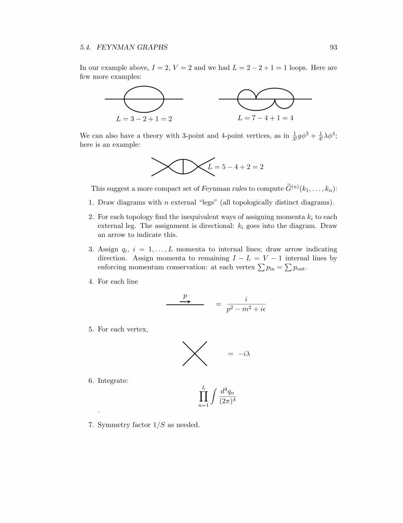
5.4. FEYNMAN GRAPHS 93
In our example above, I = 2, V = 2 and we had L = 2− 2 + 1 = 1 loops. Here arefew more examples:
L = 3− 2 + 1 = 2 L = 7− 4 + 1 = 4
We can also have a theory with 3-point and 4-point vertices, as in 13!gφ
3 + 14!λφ
4;here is an example:
L = 5− 4 + 2 = 2
This suggest a more compact set of Feynman rules to compute G(n)(k1, . . . , kn):
1. Draw diagrams with n external “legs” (all topologically distinct diagrams).
2. For each topology find the inequivalent ways of assigning momenta ki to eachexternal leg. The assignment is directional: ki goes into the diagram. Drawan arrow to indicate this.
3. Assign qi, i = 1, . . . , L momenta to internal lines; draw arrow indicatingdirection. Assign momenta to remaining I − L = V − 1 internal lines byenforcing momentum conservation: at each vertex
∑pin =
∑pout.
4. For each line
p=
i
p2 −m2 + iε
5. For each vertex,
= −iλ
6. Integrate:L∏n=1
∫d4qn(2π)4
.
7. Symmetry factor 1/S as needed.

94 CHAPTER 5. ELEMENTARY PROCESSES
5.5 Cross Section
In a common experimental setup two beams of elementary particles are acceleratedin opposite directions and brought into face to face encounter. Some fraction ofthe particles in the beams collide. The collision results in a spray of elementaryparticles emanating form the collision point and an array of detectors surroundingthe area register these outgoing particles. Here as a computer generated imageof the tracks made by charged particles that are sprayed out of the head-to-headcollision of two protons, projected onto a plane transverse to the direction of theprotons:
In another common setup a beam of particle impinges on a collection of stationarytargets. This second set-up is, of course, just the first one as seen by an observerat rest with the second “beam.” We say this observer is in the “lab frame.”
We are after a measure of how likely are these collisions to occur. The crosssection, σ, for scattering is defined through
number of collisions
unit time= (flux)× σ .
To calculate, rather than computing the number of collisions per unit time fromthe actual flux, we use unit flux (that of one-on-one particles) and therefore
collision probability
unit time= (unit flux)× σ .
We have an initial state |i〉 that consists of two particles, a final state |f〉 thatconsists of n-particles (n/ge2). The probability that |i〉 evolves into |f〉 is
Pi→f = |〈f out|i in〉|2 = |〈f in|S|i in〉|2 = |〈f |S − 1|i〉|2
where in the last step we ignore the f = i case (no collision, hence subtract 1 fromS) and suppressed the “in” label (we will get tired of carrying it around).

5.5. CROSS SECTION 95
We have to be careful to ask the right question: since we have continuumnormalization of states, if we are overly selective in what we want for |f〉, theprobability of finding it in |i〉 will vanish. Recall if you drop a pin on a piece ofpaper the probability of hitting a given point on the paper, say, (x0, y0), is zero,since a point is a set of measure zero in the set of points that comprise the area ofthe paper. Likewise, if we set |f〉 = |~k 1, . . . ,~k n〉 we’ll find Pi→f = 0. Instead weproject out a subspace of F , rather than a single state. Instead of
|〈f |S − 1|i〉|2 = 〈i|(S − 1)†|f〉〈f |S − 1|i〉
we take〈i|(S − 1)†
(∑f
some states
|f〉〈f |)
(S − 1)|i〉
In particular, for n particles in the final state we have∑f
|f〉〈f | →∫
(dk1) · · · (dkn)|~k 1, . . . ,~k n〉〈~k 1, . . . ,~k n|
where
• we may not want to sum over all possible momenta, so the integrals can berestricted
• must avoid double counting from indistinguishable particles
Suppose particles 1 and 2 are indistinguishable (but the rest are not). Then toavoid double counting one should write∑
f
|f〉〈f | → 1
2
∫(dk1) · · · (dkn)|~k 1, . . . ,~k n〉〈~k 1, . . . ,~k n|
If 1,2,3 are indistinguishable then the pre-factor becomes 1/3! since the order of~k 1, ~k 2 and ~k 3 in the label of the state is immaterial. More generally,
∑f
|f〉〈f | → 1
S
n∏i=1
(dki) |~k 1, . . . ,~k n〉〈~k 1, . . . ,~k n|
where S = m1!m2! · · · where mi is the number of identical particles of type i(∑
imi = n).We are ready to give a probability:
Pi→f =〈i|(S − 1)†
∑|f〉〈f |S − 1|i〉〈i|i〉

96 CHAPTER 5. ELEMENTARY PROCESSES
We have divided by 〈i|i〉 because states must be normalized for proper interpre-tation. Did not divide by normalization of |f〉 because it is included properly inrelativistic measure in the sum over states. We next recast this in terms of thescattering amplitude,
〈f |S − 1|i〉 = (2π)4δ(4)(Pf − Pi) iA(i→ f).
At this point we choose an initial state of plane waves with definite momentum,|i〉 = |~p1, ~p2〉. We have
〈i|i〉 = 〈~p1, ~p2|~p1, ~p2〉 = 〈~p1|~p1〉〈~p2|~p2〉
but since in general 〈~p |~k 〉 = 2E~k (2π)3δ(3)(~p−~k ), we have, 〈~p1|~p1〉 = 2E~k (2π)3δ(3)(0).This is embarrassing, but not disastrous. There are two ways of dealing with thisproblem. It is not very hard to use wave-packets, which can be properly normalized,instead of plane waves, but won’t do here; check it out in some of the textbooksin our bibliography. We have an alternative means of dealing with this problem,which is by putting the system in a finite box of volume V . We have alreadydone so in computing phase space. We discovered there that the correct interpre-tation of this infinity is (2π)3δ(3)(0)→ V . In fact, we will also use, more generally,(2π)4δ(4)(0) → V T , where T = tfinal − tinitial. So we can write 〈i|i〉 = 4E1E2V
2.Similarly
|〈f |S − 1|i〉|2 =(
(2π)4δ(4)(Pf − Pi))2|A(i→ f)|2
=(
(2π)4δ(4)(0))
(2π)4δ(4)(Pf − Pi)|A(i→ f)|2
= V T (2π)4δ(4)(Pf − Pi)|A(i→ f)|2
Putting it all together:
probability
time=
1
T
V T 1S
∫ ∏i(dki) (2π)4δ(4)(Pf − Pi)|A(i→ f)|2
4E1E2V 2
=1
V
1
4E1E2
∫|A(i→ f)|2dΦn
where
dΦn =1
S(2π)4δ(4)(Pf − Pi) (dk1) · · · (dkn)
is the Lorentz-invariant n-particle phase space.Finally, in order to determine the cross section σ we need to divide the above
by the unit flux. Assume particle 1 is uniformly distributed in a box of volumeV . The probability of finding it is a sub-volume v is v/V . We want v to be theinteraction volume, so project a volume forward of particle 2, in the direction of therelative motion ~v 2−~v 1, with cross sectional area σ perpendicular to that direction,when particle 2 moves over a time ∆t, as in the following figure:

5.5. CROSS SECTION 97
σ~v 2 − ~v 1
particle 2
|~v 2 − ~v 1|∆t
This has
volume
V=
(|~v 2 − ~v 1|∆t)σV
⇒ probability
unit time=|~v 2 − ~v 1|σ
V
Comparing with the above probability per unit time we have
dσ =1
4E1E2|~v 2 − ~v 1||A|2dΦ
where we have written dσ rather than σ to remind us that dΦ will be integratedover: σ =
∫dσ = 1
4E1E2|~v 2−~v 1|∫|A|2dΦ.
The factor E1E2|~v 2−~v 1| is invariant under boosts along the direction of ~v 2−~v 1.This is most easily seen in a frame where ~v 1 and ~v 2 are along the z-axis. Then
E1E2|~v 2 − ~v 1| = E1E2|p2
E2− p1
E1= |p2E1 − p1E2| = |ε12µνp
µ1p
ν2 |
is invariant to boosts in the 3-direction. It is useful to compute this factor in thetwo most common frames, once and for all. In the Lab frame: ~p2 = 0, E2 = m2
so E1E2|~v 2 − ~v 1| = |p2E1 − p1E2| = m2p1. In the center of mass, or CM frame,~p2 + ~p1 = 0, so that ~p1 = −~p2 ≡ ~p and E1E2|~v 2 − ~v 1| = |p2E1 − p1E2| =|~p |√
(p1 + p2)2 where p1,2 are 4-vectors. Let
s ≡ (p1 + p2)2
so that s = m21 +m2
2 + 2E1E2 + 2|~p|2. Since Ei =√|~p |2 +m2
i we have an equation
relating |~p |2 to s, which we solve:
|~p |2 =(s−m2
1 −m22)2 − 4m2
2m22
4s
This gives
4E1E2|~v 2 − ~v 1| = |~p |√s = 2
√(s−m2
1 −m22)2 − 4m2
1m22 .
The last expression is valid in any frame boosted along ~v 2 − ~v 1, and we can write
dσ =1
2√
(s−m21 −m2
2)2 − 4m21m
22
|A|2dΦ

98 CHAPTER 5. ELEMENTARY PROCESSES
Example: 2→ 2 scattering, identical particles
~p1 ~p2
~k 1
~k 2
θ
We have for identical particles m1 = m2 = m
dΦ2 =d3k1
(2π)32E1
d3k2
(2π)32E2(2π)4δ(4)(P − k1k2)
=d4k1 d
4k2
(2π)2θ(k0
1)θ(k02)δ(k2
1 −m2)δ(k22 −m2)δ(4)(P − k1k2)
Change variables:
p = k1 + k2
q = 12(k1 − k2)
⇔k1 = 1
2p+ q
k2 = 12p− q
Note that the Jacobian of the transformation,∣∣∣∂(k1,k2)∂(p,q)
∣∣∣ = 1. Then,
dΦ2 =1
(2π)2d4pδ(4)(P − p)d4qθ(1
2p0 + q0)θ(1
2p0 − q0)δ((1
2p+ q)2 −m2)δ((12p− q)
2 −m2)
=1
(2π)2d4q θ(1
2P0 − |q0|)δ(1
4P2 + P · q + q2 −m2)δ(2P · q)
In the CM frame, ~P = 0, this is simple:
dΦ2 =1
(2π)2dq0|~q |2d|~q |d cos θdφ θ(1
2P0 − |q0|)δ(1
4P2 + (q0)2 − |~q |2 −m2) 1
2P 0 δ(q0)
=1
(2π)2d cos θdφ
1
2P 012
√14(P 0)2 −m2
=1
8(2π)2d cos θdφ
√1− 4m2/s
where s = P 2 = (p1 + p2)2 as before. Therefore
dσ
d cos θdφ=
1
2
1
8(2π)2
√1− 4m2/s
1
2√
(s− 2m2)2 − 4m2|A|2
=1
32
1
(2π)2
1
s|A|2

5.6. LSZ REDUCTION, AGAIN 99
Often A is independent of φ, so
dσ
d cos θ=
1
64π
1
s|A|2
5.6 LSZ reduction, again
We want to establish the LSZ reduction formula. We don;t pretend to give a com-plete proof. The objective is to express the S-matrix in terms of Green’ s functions,vacuum expectation values of time ordered products, of in fields. Consider
out〈ψ|~k 1,~k 2, . . . ,~k n〉in = out〈ψ|~k 1χ〉in = out〈ψ|α†~k 1inχ〉in
Recall
φin(x) =
∫(dq)
(α~q ine
−iq·x + α†~q ineiq·x)
∂tφin(x) =
∫(dq)
(−iE~qα~q ine
−iq·x + iE~qα†~q ine
iq·x)
Inverting these,
α†~q in = −i∫d3x e−iq·x
←→∂t φin(x)
So we have
out〈ψ|~k 1χ〉in = −i∫d3x e−ik1·x
←→∂t out〈ψ|φin(x)|χ〉in
= −iZ−12
∫d3x e−ik1·x
←→∂t out〈ψ|φ(x)|χ〉in as t→ −∞.
Now we use the fundamental theorem of calculus, g(t2) = g(t1) +∫ t2t1dtdgdt , with
t2 →∞ and t1 → −∞ so that
limt→−∞
∫d3x e−ik1·x
←→∂t out〈ψ|φ(x)|χ〉in = lim
t→∞
∫d3x e−ik1·x
←→∂t out〈ψ|φ(x)|χ〉in
−∫d4x ∂t
(e−ik1·x
←→∂t out〈ψ|φ(x)|χ〉in
)The first term on the right hand side times −iZ−
12 is out〈ψ|α†~k 1out
|χ〉in, as can
be seen by reversing the steps. If |ψ〉out = |~p1, ~p2, . . . , ~pn′〉out then α†~k 1out|ψ〉out =
(2π)32E~k 1δ(3)(~k 1−~p1)|~p2, . . . , ~pn′〉out+· · ·+(2π)32E~k 1
δ(3)(~k 1−~pn′)|~p1, . . . , ~pn′−1〉out
corresponds to a particle not participating in the scattering. We have no use

100 CHAPTER 5. ELEMENTARY PROCESSES
for this. For the second term on the right hand side we use ∂t(f(t)←→∂t g(t)) =
f∂2t g − (∂2
t f)g so it is
−∫d4x e−iq·x(∂2
t + E2~q ) out〈ψ|φ(x)|χ〉in
Using E2~q e−iq·x = (|~q |2 + m2)e−iq·x = (−~∇2 + m2)e−iq·x and integrating by parts
we have finally
out〈ψ|~k 1χ〉in = out〈ψ|α†~k 1out|χ〉in + iZ−
12
∫d4x e−ik1·x(∂2 +m2) out〈ψ|φ(x)|χ〉in
Similarly
out〈ψ~p |χ〉in = out〈ψ|α†~p in|χ〉in + iZ−12
∫d4x eip·x(∂2 +m2) out〈ψ|φ(x)|χ〉in (5.11)
We woud like to repeat the process until we remove all particles from |ψ〉out
and |χ〉in. To see how this goes move a particle off from |χ〉in from what we alreadyhad:
out〈ψ|φ(0)|~kχ′〉in = out〈ψ|φ(0)α†~k in|χ′〉in = −iZ−
12 limx0→−∞
∫d3x e−ik·x
←→∂x0out〈ψ|φ(0)φ(x)|χ′〉in
= iZ−12
∫d4x ∂x0
(e−ik·x
←→∂x0 out〈ψ|φ(0)φ(x)|χ′〉in
)− iZ−
12 limx0→∞
∫d3x e−ik·x
←→∂x0out〈ψ|φ(0)φ(x)|χ′〉in (5.12)
In the last expression we would like to move φ(x) to the left of φ(0) so that we
may turn φ(x) as x0 → ∞ into α†~koutacting on 〈out|. To this end we rewrite the
first term in the last expression in (5.12) using
φ(0)φ(x) = (θ(−x0) + θ(x0))φ(0)φ(x) + θ(x0)(φ(x)φ(0)− φ(x)φ(0))
= T (φ(x)φ(0)) + θ(x0)[φ(0), φ(x)]
Then in ∫d4x ∂x0
(e−ik·x
←→∂x0 out〈ψ|θ(x0)[φ(0), φ(x)]|χ′〉in
)(5.13)
when←→∂x0 hits θ(x0) we get the equal time commutator [φ(0), φ(x)] = 0. So we
have (5.13) is
=
∫d4x ∂x0
[θ(x0)
(e−ik·x
←→∂x0 out〈ψ|[φ(0), φ(x)]|χ′〉in
)]= lim
x0→∞
∫d3x e−ik·x
←→∂x0 out〈ψ|[φ(0), φ(x)]|χ′〉in

5.7. PERTURBATION THEORY, AGAIN 101
Combining this with the last term in (5.12) gives precisely what we want: it reversesthe order of φ(0)φ(x) so that
out〈ψ|φ(0)|~kχ′〉in = iZ−12
∫d4x
(e−ik·x(∂2 +m2) out〈ψ|T (φ(0)φ(x))|χ′〉in
)+out〈ψ|α†~kout
φ(0)|χ′〉in
We thus arrive at
out〈ψ|~k 1~k 2χ
′〉in = (iZ−12 )2
∫d4x1d
4x2e−ik1·x1−ik2·x2
× (∂2x1 +m2)(∂2
x2 +m2) out〈ψ|T (φ(0)φ(x))|χ′〉in + disconnected
One can repeat the process until all particles in |in〉 are removed and we are leftwith |0〉in = |0〉. The argument above can be streamlined by replacing T (φ(0)φ(x))for φ(0)φ(x) in the line above (5.12)), and this indeed becomes very convenient incompleting the argument for arbitrary number of particles.
Similarly we can remove 1-particle states from out〈~kψ| using (5.11) repeatedly.
5.7 Perturbation theory, again
We now give a proof of (5.6) that gives us the basis for perturbation theory. Con-sider
G(n)(x1, . . . , xn) = 〈0|T (φ(x1) · · ·φ(xn))|0〉 .
Take for definiteness x01 ≥ x0
2 ≥ · · · ≥ x0n. Recall φ(x) = U(t)−1φinU(t), ans use
this in each φ in the Green’s function:
G(n)(x1, . . . , xn) = 〈0|U−1(t1)φ(x1)U(t1)U−1(t2)φ(x2)U(t2) · · ·U−1(tn)φ(xn)U(tn)|0〉 .
Let U(t, t′) = U(t)U−1(t′). This satisfies
U(∞,−∞) = S (5.14)
U(t,−∞) = U(t) (5.15)
U(t, t′)U(t′, t′′) = U(t, t′′) (5.16)
Moreover,
i∂U(t, t′)
∂t= H ′inU(t, t′), with U(t′, t′) = 1 .
This is the same equation satisfied by U(t), but with a different boundary condition.So the solution is the same only with different limits of integration,
U(tf , ti) = T exp
(−i∫ tf
ti
dtH ′in(t)
).

102 CHAPTER 5. ELEMENTARY PROCESSES
We now have
G(n) = 〈0|U−1(∞)U(∞, t1)φin(x1)U(t1, t2)φin(x2)U(t2, t3) · · ·U(tn−1, tn)φin(xn)U(tn,−∞)U(−∞)|0〉= 〈0|U−1(∞)T (U(∞, t1)φin(x1)U(t1, t2)φin(x2)U(t2, t3) · · ·U(tn−1, tn)φin(xn)U(tn,−∞)) |0〉= 〈0|U−1(∞)T (U(∞, t1)U(t1, t2)U(t2, t3) · · ·U(tn−1, tn)U(tn,−∞)φin(x1)φin(x2) · · ·φin(xn)) |0〉= 〈0|U−1(∞)T (U(∞,−∞)φin(x1)φin(x2) · · ·φin(xn)) |0〉
Uniqueness of the vacuum means that |0〉, |0〉in, |0〉out, are equal up to a phase.Moreover, U(∞)|0〉 = S|0〉 must be |0〉 up to a phase. To see this note that Scommutes with Poincare transformations, U(aµ,Λ)SU †(aµ,Λ) = S and |0〉 is theunique state (up to a phase) that is left invariant by a Poincare transformation.Then U(aµ,Λ)(S|0〉) = U(aµ,Λ)SU †(aµ,Λ)U(aµ,Λ)|0〉 = S|0〉 so S|0〉 is invariantand hence equal to |0〉 up to a phase. So we have 〈0|U−1(∞) = 〈0|U−1(∞)|0〉 〈0|.Using this and
U(∞) = U(∞,−∞) = T exp
(−i∫ ∞−∞dtH ′in(t)
)we finally have
G(n)(x1, . . . , xn) =in〈0|T
(φin(x1) · · ·φin(xn)ei
∫d4xL′in
)|0〉in
in〈0|T(ei
∫d4xL′in
)|0〉in
Note that we replaced |0〉in for |0〉 since the phases in numerator and denominatorcancel.
This is not what we set out to prove. It is better. The denominator correspondsto a set of graphs without external legs. These vacuum graphs can also appear inthe numerator, just multiplying any graph with external legs. It is a simple exerciseto check that the vacuum graphs in the numerator are cancelled by the graphs inthe denominator.
5.7.1 Generating Function for Green’s Functions
LetZ[J ] = 〈0|Tei
∫d4x J(x)φ(x)|0〉 .
Then
G(n)(x1, . . . , xn) =1
i
δ
δJ(x1)· · · 1
i
δ
δJ(xn)Z[J ]
∣∣∣∣J=0
and
Z[J ] =in〈0|Tei
∫d4x(L′in+J(x)φin(x))|0〉in
in〈0|T(ei
∫d4xL′in
)|0〉in

5.7. PERTURBATION THEORY, AGAIN 103
This is a convenient way of summarizing the results above for G(n), all n. Notealso that
Z[J ] =∑n
in
n!
∫d4x1 · · · d4xn J(x1) · · · J(xn)G(n)(x1, . . . , xn) .
5.7.2 Generating Function for Connected Green’s Functions
Similarly we define
W [J ] =∑n
in
n!
∫d4x1 · · · d4xn J(x1) · · · J(xn)G(n)
conn(x1, . . . , xn) .
We will now show that Z[J ] = eiW [J ].
We use a diagrammatic notation to see how this works:
+W [J ] = + · · ·
where the heavy dots ffl stand for J(x), the hatch circles with n lines stand for G(n)
and an integral 1n!
∏i
∫d4xi in each term is understood. Let streamline notation for
the purposes of this proof: remove the heavy dots (the ends of lines are understoodas having them) and reduce the hatch circle to a point, so that the above figure isthe same as
+W [J ] = + · · ·
With this notation we consider the exponential of W [J ]:
exp(W [J ]) = exp( )
exp( )
exp( )
· · ·
Now expand its exponential, as in
exp( )
= 1 + + +12! + · · ·1
3!
and reorganize by powers of J , that is, number fo external legs:

104 CHAPTER 5. ELEMENTARY PROCESSES
expW [J ] = 1 + + + +(
12!
)+ · · ·
where the ellipses stand for terms with five or more legs. Let’s analyze in moredetail the term in parenthesis: we want to show that it gives G(4) (times sources,1/4! and integrated). The “cross” stands for
1
4!
∫d4y1 · · · d4y4 J(y1) · · · J(y4)G(4)
conn(y1, . . . , y4)
Now, δ4
δJ(x1)···δJ(x4) of this gives G(4)conn(x1, . . . , x4). Note that the 4! is absent since
there are 4! terms from the integral (same as in d4
dx4x4 = 4!). Turning to the other
term, the disconnected graph, we have
δ4
δJ(x1) · · · δJ(x4)
1
2!
(1
2!
∫d4yd4z J(y)J(z)G(2)(y, z)
)2
= G(2)(x1, x2)G(2)(x3, x4) +G(2)(x1, x3)G(2)(x2, x4) +G(2)(x1, x4)G(2)(x2, x3)
If we take the for J-functional derivatives and set J = 0 these are the only termswe pick up in the expansion, so we have
δ4
δJ(x1) · · · δJ(x4)eW [J ]
∣∣∣J=0
= G(4)conn(x1, . . . , x4)
+G(2)(x1, x2)G(2)(x3, x4) +G(2)(x1, x3)G(2)(x2, x4) +G(2)(x1, x4)G(2)(x2, x3)
= G(4)(x1, . . . , x4) =δ4
δJ(x1) · · · δJ(x4)Z[J ]
∣∣∣J=0
In the general case, the term with Jn in eW [J ] is a sum of all possible contri-butions of the form
1
n2!
(1
2!
∫J1J2G
(2)c
)n2 1
n3!
(1
3!
∫J1J2J3G
(3)c
)n3
· · ·
such that 2n2 + 3n3 + · · · = n, in a hopefully obvious condensed notation. Forexample, n = 4 has (n2 = 2, n6=2 = 0) + (n4 = 1, n6=4 = 0), and n = 6 has (n6 =1, n6=6 = 0) + (n4 = 1, n2 = 1, n6=4,2 = 0) + (n3 = 2, n6=3 = 0) + (n2 = 3, n6=2 = 0).
Consider the term with G(k)c : take
δknk
δJ(x1) · · · δJ(xknk)
1
nk!
(1
k!
∫J1 · · · JkG(k)
c
)nk

5.7. PERTURBATION THEORY, AGAIN 105
This is completely symmetric under permutations of x1, . . . , xknk . To make thisexplicit we rewrite it as
1
nk!
(1
k!
∫J1 · · · JkG(k)
c
)nk=
1
nk!
1
(k!)nk
×∫ knk∏
i=1
d4yi J(y1) · · · J(yknk)G(k)c (y1, . . . , yk) · · ·G(k)
c (y(nk−1)k+1, . . . , ynkk)
Taking knk J-derivatives we obtain
1
nk!
1
(k!)nkG(k)c (x1, . . . , xk) · · ·G(k)
c (x(nk−1)k+1, . . . , xnkk)+permutations of x1, . . . , xnkk
This contains many repeated terms. We need to count the number of inequivalent
permutations. For each G(k)c there are k! equivalent permutations of the arguments;
this gives (k!)nk . Then we can permute the G(k)c among themselves; there are nk!
such permutations. So we obtain
δknk
δJ(x1) · · · δJ(xknk)
1
nk!
(1
k!
∫J1 · · · JkG(k)
c
)nk= G(k)
c (x1, . . . , xk) · · ·G(k)c (x(nk−1)k+1, . . . , xnkk) + inequiv-perms
Finally combine all terms and symmetrize over x1, . . . , xn. We obtain all possiblecombinations of Gc’s that can make G(n). But that is precisely what we intendedto show.
Chapter 6
Fields that are not scalars
6.1 Generalities
So far we have concentrated our studies on fields that transform very simply underLorentz transformations. Brief review: we want φ(x) to correspond to φ′(x′) whenx′ = Λx. For a scalar field “correspond to” means they are equal, φ′(x′) = φ(x).Tha is,
φ′(x) = φ(Λ−1x) .
Less trivial is the case of a vector field, Aµ(x). We can obtain it from tak-ing a derivative on the scalar field which gives, ∂µφ
′(x) = ∂νφ(Λ−1x)(Λ−1)νµ =Λµ
ν∂νφ(Λ−1x). This holds for any vector so
A′µ(x′) = ΛµνAν(x) or A′µ(x) = ΛµνA
ν(Λ−1x) .
We can generalize this to other tensors easily, by considering tensor products ofvectors, e.g.,
B′µνλ(x) = ΛµρΛνσΛλδB
ρσδ(Λ−1x)
In general, a collection of fields ψα, α = 1, . . . , n transforms as
ψ′α(x) = Dαβ(Λ)ψβ(Λ−1x) , (6.1)
where Dαβ is an n × n matrix function of Λ. If ψ′α(x′) = Dαβ(Λ1)ψβ(x) withx′ = Λ1x and ψ′′α(x) = Dαβ(Λ2)Dβγ(Λ1)ψγ(Λ−1
1 Λ−12 x). This should equal the
transformation with x′′ = Λ2Λ1x, ψ′′α(x) = Dαβ(Λ2Λ1)ψβ((Λ2Λ1)−1x). This im-poses a requirement on the functions D(Λ) that they furnish a representation ofthe Lorentz group:
D(Λ2)D(Λ1) = D(Λ2Λ1) (6.2)
106

6.1. GENERALITIES 107
It suffices to understand the irreducible representations. Brief review/introduction.If D is a representation, so is SDS−1 for any invertible matrix S. If we can findan S such that SDS−1 is block diagonal for all Λ,
D(1) 0 · · · 0
0 D(2) · · · 0
0 0. . . 0
0 0 · · · D(N)
then we say D is reducible (to be more precise, the case that D(1) is the onlyblock in the block diagonal matrix should be excluded). Else, it is irreducible.If D is reducible it (or, rather, SDS−1 for some S) can be written as the directsum of irreducible representations D(i), i = 1, . . . , N , and we write this as D =D(1)⊕D(2)⊕· · ·⊕D(N). The point is that one can form any reducible representationfrom knowledge of the possible irreducible ones. So we need only determine thefields that correspond to irreducible representations,
ψ′(1)(x) = D(1)(Λ)ψ(1)(Λ−1x), . . . , ψ′(N)(x) = D(N)(Λ)ψ(1)(Λ−1x) ,
and the whole collection transforms as a reducible representationψ′(1)(x)
ψ′(2)(x)...
ψ′(N)(x)
=
D(1) 0 · · · 0
0 D(2) · · · 0
0 0. . . 0
0 0 · · · D(N)
ψ(1)(Λ−1x)
ψ(2)(Λ−1x)...
ψ(N)(Λ−1x)
An example: a pair of scalars, φ1, φ2, a vector, Aµ, and a tensor, Tµν , with thetransformations given above.
If D acts on d dimensional vectors we say the dimension of D is d, dim(D) = d.(Aside: The representations may be double valued. You have seen this in QM.
A spin-12 wave-function, ψ =
(ψ1
ψ2
)transforms, under rotations by an angle θ about
the n axis, by ψ → ei12θn·~σψ. That is D(R) = ei
12θn·~σ is a 2-dim representation of
the rotation R by an angle θ about the n axis. But R is the same for θ = 0 andθ = 2π, and eiπn·~σ = −1.)
If D(Λ) is a representation, so is D∗(Λ). Proof: take the complex conjugateof D(Λ1)D(Λ2) = D(Λ1Λ2). Clearly, dim(D∗) = dim(D). D∗ may or may not beequivalent to D.
If D(1) and D(2) are representations, so is the tensor product, D(1) ⊗ D(2).The tensor product is defined as always: if D(1) acts on ψ(1), D(2) on ψ(2), thenD(1)⊗D(2) acts on ψ(1)⊗ψ(2) according to (D(1)⊗D(2))(ψ(1)⊗ψ(2)) = (D(1)ψ(1))⊗

108 CHAPTER 6. FIELDS THAT ARE NOT SCALARS
(D(2)ψ(2)). If d = dim(D) and d′ = dim(D′) then dim(D ⊕ D′) = d + d′ anddim(D⊗D′) = dd′. Generally, D⊗D′ is reducible, D⊗D′ = D(1)⊕D(2)⊕· · ·⊕D(N),with d1 + d2 + · · · + dN = dd′. An example is a two index tensor. It canbe obtained from the tensor product of two vectors, Cµν = AµBν , and is areducible representation: under Lorentz transformations the trace ηµνC
µν , theanti-symmetric part, C [µν] = 1
2(Cµν − Cνµ), and the symmetric traceless part,
Cµν − 14η
µνηλσCλσ = 1
2(Cµν + Cνµ) − 14η
µνηλσCλσ do not mix into each other.
Moreover, one can show that the 6-dimensional antisymmetric 2-index tensor isitself the direct sum of two 3-dimensional irreducible representations, satisfyingCµν± = ±1
2εµνλσC
λσ± (these are said to be self-dual and anti-self-dual, respectively).
The 4 × 4 = 16-dimensional tensor product of two 4-vectors splits into four irre-ducible representations of dimension 1, 3, 3, and 9, as we have just seen. With aslight abuse of notation, this is 4⊗ 4 = 1⊕ 3⊕ 3′ ⊕ 9.
Here is the point. We can build up every irreducible representation (and fromthem every reducible representation, hence every representation) by starting fromsome small basic representations, and taking their tensor products repeatedly:these tensor products are direct sums of new irreducible representation, and themore basic representations we tensor-product the higher the dimension of the newirreducible representations we will find.
It turns out, as we will show below, the representations of the Lorentz groups arelabeled by two half-integers, (s+, s−) and have dimension (2s+ + 1)(2s−+ 1). Thisis because the Lorentz group (or rather, its algebra) is isomorphic to two copies ofspin, SU(2)×SU(2), and as you know from particle QM the representations of spinare classified by half integer s = 0, 1
2 , 1, . . . and have dimension 2s+ 1 = 1, 2, 3, . . .correspondingly. For example, (0, 0) is a 1-dimensional representation, the scalar,(1
2 ,12) is a 4-dimensional representation, corresponding to vectors, Aµ. For the
tensor product of two vectors, we need first, from QM, that 12 ⊗
12 = 0 ⊕ 1. So
(12 ,
12)⊗(1
2 ,12) = (0, 0)⊕(1, 0)⊕(0, 1)⊕(1, 1). The two 3-dimensional representations
associated with the antisymmetric tensor correspond to (1, 0) and (0, 1) and the9-dimensional symmetric traceless tensor is (1, 1).
6.2 Spinors
Back to Lorentz group and physics. Question: other than scalars and tensors, whatother representations of the Lorentz group do we have? Answer: spinors and theirtensor products. Let σµ = (σ0, σi), where
σ0 =
(1 00 1
), σ1 =
(0 11 0
), σ2 =
(0 −ii 0
), σ3 =
(1 00 −1
).

6.2. SPINORS 109
Let
P = pµσµ =
(p0 − p3 −p1 + ip2
−p1 − ip2 p0 + p3
).
Then det(P ) = p2 = ηµνpµpν . Then for any unimodular 2 × 2 matrix M we have
det(M †PM) = det(P ). Since any hermitian matrix can be expanded in terms of
σµ with real coefficients and P ′ = M †PM is hermitian (if P is), then P ′ = p′µσµ
with p′2 = p2. That is, M = M(Λ) induces a Lorentz transformation.
Now M(Λ) does not satisfy the representation defining equation (6.2). If p′′ =
Λ2p′ and p′ = Λ1p then P ′′ = M †(Λ2)P ′M(Λ2) = M †(Λ2)M †(Λ1)PM(Λ1)M(Λ2)
and this should correspond to p′′ = Λ2Λ1p or P ′′ = M †(Λ2Λ1)PM(Λ2Λ1). Com-paring we see that,
M(Λ1)M(Λ2) = M(Λ2Λ1) .
Defining M(Λ) = M(Λ−1) we obtain a representation,
M(Λ2)M(Λ1) = M(Λ−12 )M(Λ−1
1 ) = M(Λ−11 Λ−1
2 ) = M((Λ2Λ1)−1) = M(Λ2Λ1) .
So M(Λ) gives a 2-dimensional representation of Λ. It acts on 2-dimensionalspinors (vectors in a 2-dimensional space):
ψ′α = Mαβ(Λ)ψβ
If P ′ = M †PM with P ′ = p′νσν = Λν
µpµσν then equating this to M †PM for
arbitrary pµ we must have
M(Λ)†σµM(Λ) = Λνµσν = (Λ−1)µνσ
ν (6.3)
orM(Λ)†σµM(Λ) = Λµνσ
ν (6.4)
As we have seen, the complex conjugate, M∗(Λ), must also be a representation.It satisfies,
MTσµ∗M∗ = Λµνσν∗
or sandwiching with σ2 —a similarity transformation— and defining σµ = σ2σµ∗σ2 =(σ0,−σi), and M = σ2M∗σ2:
M†σµM = Λµν σ
ν
So there must be a 2-dimensional representation of the Lorentz group, of 2-component vectors, or spinors, that transform according to
ψ′α(x) = Mαβ(Λ)ψβ(Λ−1x)

110 CHAPTER 6. FIELDS THAT ARE NOT SCALARS
and also a complex conjugate representation that acts on other 2-component vec-tors, also called a spinors, that transform according to
χ′α(x) = Mαβ(Λ)χβ(Λ−1x) .
It is convenient to arrange the spinors into 2-component column vectors, and write
ψ′ = M(Λ)ψ and χ′ = M(Λ)χ
Note thatψ′†σµψ′ = ψ†M †σµMψ = Λµν ψ
†σνψ .
andχ′†σµχ′ = χ†M
†σµMχ = Λµν χ
†σνχ .
In making tensors out of these it is convenient to distinguish the indices in ψ andχ, so we write ψα and χα (still with α = 1, 2 and α = 1, 2).
We can construct a scalar out of two spinors, ψ1 and ψ2:
ψ′T1 σ2ψ′2 = ψT1 M
Tσ2Mψ2 = ψT1 σ2ψ2 (6.5)
The last step follows from
(MTσ2M)αβ = −iεγδMαγMβδ
= −iεαβ det(M)
= σ2αβ
Similarly, χT1 σ2χ2 is a scalar. Note that ψ†1ψ2 is not a scalar since M is not generally
unitary. Note also that ψTσ2ψ = 0, so we cannot make a scalar out of a single ψ.Form Eq. (6.4) we can verify that
M = exp(− i
2~α · ~σ)
= cos(12α)− iα · ~σ sin(1
2α) (6.6)
is a representation of Λ = R = a rotation by angle α about an axis in the α = ~α/αdirection, and
M = exp(
12~β · ~σ
)= cosh(1
2β) + β · ~σ sinh(12β)
is a representation of a boost by velocity β, that is, a representation of
Λ =
(γ γβγβ γ
)where γ = 1/
√1− β2, ~β is along the x axis, and the last two rows and columns
of Λ have been omitted. By complex conjugating it follows that
M = exp(− i
2~α · ~σ)
(6.7)
6.3. A LAGRANGIAN FOR SPINORS 111
is a representation of the same rotation R (a rotation by angle α about α), and
M = exp(−1
2~β · ~σ
)is a representation of a boost by velocity ~β .
6.3 A Lagrangian for Spinors
We want to construct a Lagrangian density for spinors. We put the general con-straints:
(i) Constructed from ψ and ψ† and their first derivatives ∂µψ and ∂µψ†.
(ii) Real, L∗ = L (or for quantum fields, hermitian, L† = L).
(iii) Lorentz invariant (at least up to total derivatives)
(iv) At most quadratic in the fields.
The last condition is not generally necessary. We impose it for simplicity. Higherorders in the fields will correspond to interactions.
From (iv) we need to construct L from bilinears ψ† ⊗ ψ and ψ ⊗ ψ. We knowwe can form a vector out of these, but not a scalar. Now,
∂µψ(Λ−1x) = ∂µ((Λ−1)νλxλ)(∂νψ)(Λ−1x) = (Λ−1)νµ(∂νψ)(Λ−1x) ,
so that
ψ′†σµ∂µψ′ = ψ†M †σµM(Λ−1)νµ∂νψ = ψ†Λµλσ
λM(Λ−1)νµ∂νψ = ψ†σµ∂µψ .
Both ψ†σµ∂µψ and ∂µψ†σµψ transform as scalars so they are candidates for an
invariant Lagrangian. But the sum is a total derivative, ∂µ(ψ†σµψ) so it is irrelevant(it does not contribute to the equations of motion). So we take the difference,
12ψ†σµ←→∂µψ = 1
2
(ψ†σµ∂µψ − ∂µψ†σµψ
)as a possible term in the Lagrangian. It’s complex conjugate is
12(ψ†σµ
←→∂µψ)∗ = 1
2
(ψTσµ∗∂µψ − ∂µψTσµ∗ψ∗
)= 1
2
(∂µψ
†σµ†ψ − ψ†σµ†∂µψ)
= −12ψ†σµ←→∂µψ

112 CHAPTER 6. FIELDS THAT ARE NOT SCALARS
If we take L = A12ψ†σµ←→∂µψ then for L∗ = L we must have A = ±i|A|. Redefining
ψ → 1√|A|ψ we have a candidate Lagrangian density
L = ±1
2ψ†σµ i
←→∂µψ
We will see below how to choose properly between the two signs. Note that if werelax assumption (iv) we could add other terms, e.g., (ψ†σµψ)(ψ†σµψ).
Equations of motion: recall, with a complex field we can take variations withrespect to ψ and ψ† separately, as if they were independent variables. Now in theaction integral it is convenient to integrate by parts, so that∫
d4xL = ±∫d4x
1
2ψ†σµ i
←→∂µψ = ±
∫d4xψ†σµ i∂µψ
Then, trivially,δLδψ†
= 0 ⇒ σµ∂µψ = 0 .
This is
(σ0∂0 + σi∂i)ψ = 0 ⇒ ∂0ψ = −σi∂iψ = −~σ · ~∇ψ
so that
∂20ψ = −∂0~σ · ~∇ψ = −~σ · ~∇∂0ψ = (~σ · ~∇)2ψ = ∇2ψ
This is precisely the KG equation with m = 0
∂2ψ = (∂20 −∇2)ψ = 0 .
Each component of ψ satisfies the massless KG equation.
We can construct a Lagrangian for fields in the complex conjugate representa-tion, χ. An analogous argument gives us
L = ±χ†σµ i∂µχ
with equation of motion
σµ∂µχ = 0
This again gives ∂2χ = 0 but now with ∂0χ = ~σ · ~∇χ (note the sign difference).
Plane wave expansion. Since these are complex fields we have different coeffi-cients for the positive and negative energy components:
ψα =
∫(dk)
[e−ik·xB~k ,α + eik·xD~k ,α
]

6.3. A LAGRANGIAN FOR SPINORS 113
where B~k ,α and D~k ,α are two component operator valued objects. Since ∂2ψ = 0
we must have k2 = E2~k− ~k 2 = 0, that is, k0 = E~k = |~k | as we should for
massless particles. But the equation of motion is first order in derivatives. Using∂µe∓ik·x = ∓ikµe∓ik·x we have∫
(dk)[e−ik·xkµσ
µB~k − ei·xkµσ
µD~k
]= 0
That is, we need(k0 − k3 −k1 + ik2
−k1 − ik2 k0 − k3
)(B~k ,1B~k ,2
)= 0
(k0 − k3)B~k ,1 = −(−k1 + ik2)B~k ,2
(−k1 − ik2)B~k ,1 = −(k0 + k3)B~k ,2
and similarly for D~k ,α. Let
u~k = N~k
(k1 − ik2
k0 − k3
).
N~k is a normalization factor. We could choose it to have, for example, u†~ku~k = 1,
but we will wait to choose it conveniently later. Note that since k2 = 0 we can alsowrite this as
u~k = N~kk0 − k3
k1 − ik2
(k0 + k3
k1 + ik2
)= N ′~k
(k0 + k3
k1 + ik2
).
For the plane wave-expansion of χ we need to solve kµσµv~k = 0. But this is
just like the equation for u~k only replacing −~k for ~k . So v~k = u−~k up to a phase.Since there is only one solution to the matrix equation, we rewrite our plane waveexpansion as
ψ =
∫(dk)
[e−ik·xβ~ku~k + eik·xδ†~k
u~k
]where now the operators β~k and δ~k are one-component objects. So other than thespinor coefficient u~k this expansion looks very much like the one for complex scalarfields.
6.3.1 Hamiltonian; Fermi-Dirac Statistics
Let’s compute the Hamiltonian. This should allow us to fix the sign in the La-grangian density since we want a Hamiltonian that is bounded from below. Fromthe density
H =∂L
∂(∂tψ)∂tψ − L = ∓iψ†~σ · ~∇ψ

114 CHAPTER 6. FIELDS THAT ARE NOT SCALARS
we obtain the Hamiltonian in terms of creation/annihilation operators,
H = ∓∫
(dk)(dk′)u†~k ′~σ ·~ku~k
[(2π)3δ(~k ′ − ~k )(δ~k ′δ
†~k− β†~k ′β~k ) + (2π)3δ(~k ′ + ~k )(β†~k ′
δ†~k− δ~k ′β~k )
]Now use, kµσ
µu~k = 0 or
~k · ~σu~k = E~ku~k with E~k = |~k |,
and adopt the normalizationu†~ku~k
= 2E~k .
Moreover, from the explicit form of u~k we have
u†~ku−~k
= 0
Putting these together we have
H = ∓∫
(dk)E~k
(−β†~kβ~k + δ~k
δ†~k
)If we take, as we have done before,
[β~k, β†~k ′
] = (2π)32E~k δ(3)(~k − ~k ′) = [δ~k
, δ†~k ′] (6.8)
then
H = ∓∫
(dk)E~k
(−β†~kβ~k + δ†~k
δ~k
)plus an infinite constant that we throw away (normal ordering). We were hopingto fix the sign, but instead we encounter a disaster! If we choose the − sign in thedefinition of L the β†~k
β~khas a spectrum unbounded from below while if we choose
the + sign the δ†~kδ~k
term is unbounded form below.
But if instead of (6.8) we choose anti-commutation relations,
β~k , β†~k ′ = (2π)32E~k δ
(3)(~k − ~k ′) = δ~k , δ†~k ′ (6.9)
where A,B ≡ AB +BA, then up to an infinite constant
H = ±∫
(dk)E~k
(β†~kβ~k
+ δ†~kδ~k
)This is bounded from below only if we take the + sign in L, unbounded form belowotherwise. This fixes the sign,
L = ψ† iσµ∂µψ ,

6.3. A LAGRANGIAN FOR SPINORS 115
and furthermore tells us that the fields anti-commute,
ψ†(x), ψ(y)|x0=y0 = δ(3)(~x − ~y )
The Fock space consists of particles β†~k|0〉 and antiparticles, δ†~k
|0〉. Two particle
states satisfy |~k 1,~k 2〉 = β†~k 1β†~k 2|0〉 = −β†~k 2
β†~k 1|0〉 = −|~k 2,~k 1〉, so the wave function
is anti-symmetric; so are β†~k 1δ†~k 2|0〉 and δ†~k 1
δ†~k 2|0〉. We have discovered Fermi-Dirac
statistics! Moreover, we were forced into it by consistency of the theory. Thisspin-statistics connection is a theorem in QFT, rather than an ad-hoc rule as inparticle QM.
A note on the normalization of u~k . It seems that we chose it as 2E~k to givethe Hamiltonian as the sum of E~k times the number of modes. Actually, we
should fix the normalization to give ψ†(x), ψ(y)|x0=y0 = iδ(3)(~x − ~y ) given thatcreation/annihilation operators satisfy (6.9). It is a simple exercise to check thatthis is the case:
ψ†α(x), ψβ(y)|x0=y0 =
∫(dk)ei
~k ·~k[u∗~kαu~kβ + v∗~kαv~kβ
]where we have used v~k = u−~k . We can now check by direct computation that
u~ku†~k
+ v~kv†~k
= 2E~k1 (6.10)
giving the desired result. The relation (6.10) is in fact a completeness relation,
∑ |n〉〈n|〈n|n〉
= 1 isu~ku†~k
+ v~kv†~k
2E~k
= 1
Helicity(η).
Helicity of a state is defined as the angular momentum along the direction ofmotion. Take a particle moving along the z-axis, k1 = k2 = 0, k3 = ±k0. Then ifthe particle moves in the z direction, k3 = k0
u(+) ∝(
10
),
while if it moves in the negative z-direction, k3 = −k0,
u(−) ∝(
01
).

116 CHAPTER 6. FIELDS THAT ARE NOT SCALARS
For a rotation by α about the z-axis, Eq. (6.6) gives
M
(10
)= e−iα/2
(10
)and M
(01
)= eiα/2
(01
),
so that u(±) are eigenvectors of M with eigenvalues e∓iα/2. But
M = e−iαJ3
so u(+) is an eigenvector of η = k · ~J = J3 with eigenvalue, or helicity, η = 12 while
u(−) has η = k · J = −J3 so again η = 12 .
(Aside: In general
Jµν = Lµν + Sµν =
∫d3x [xµT 0ν − xνT 0µ − iπJ µνφ]
where φ′(x) = (1− i2ωµνJ
µν)φ(x−ωx) and π is the canonical momentum conjugateto φ. For the complex case one must sum over π and π†. For spinors we only haveπ = ∂L/∂(∂tψ) = ψ† iσ0 = iψ†, since π† = ∂L/∂(∂tψ
†) = 0. So for spinors,Sµν =
∫d3xψ†Mµνψ. If U = exp(− i
2ωµνJµν), then infinitesimally Uφ(x)U † =
(1 − i2ωµνJ
µν)φ(x − ωx). For a rotation about the z-axis by angle θ take ω12 =−ω21 = θ, so that U = exp(−iθJ3). This can be verified from UAλ(0)U † =(ηλσ + ωλσ)Aσ(0):
A′1 = A1 + ω12A2 = A1 − ω12A2 = A1 − θA2
A′2 = A2 + ω21A1 = A2 − ω21A1 = A2 + θA1 .
The factor of 2 in the definition of the spin part, Sµν , is correct. This can bechecked with the vector representation, for which (J µν)λσ = −i(δµλδ
νσ−δνλδ
µσ). End
aside).To determine the helicity of 1-particle states annihilated and created by ψ, it
is convenient to project these states into or out of the vacuum. Consider then atransformation U(R) by a rotation R by angle α about the z-directions and a statewith momentum ~k = kz:
〈0|U(R)ψ(0)U †(R)|kz〉 = 〈0|M(R)ψ(0)|kz〉
The right hand side picks up only the contribution in the plane wave expansionfrom the annihilation operator with momentum ~k = kz, so the matrix M actson this spinor giving a factor of exp(−iα/2). On the left hand side we have〈0|ψ(0)(U †(R)|kz〉). Since R does not change ~k = kz, the state can change at mostby an overall phase. Comparing we read off the phase, U †(R)|kz〉 = exp(−iα/2)|kz〉or U(R)|kz〉 = exp(iα/2)|kz〉. But U(R) = exp(−iαJ3) = exp(−iαη), so the state

6.3. A LAGRANGIAN FOR SPINORS 117
annihilated by ψ has η = −12 . Similarly, 〈kz|U(R)ψ(0)U †(R)|0〉 = 〈kz|Mψ(0)|0〉 =
exp(−iα/2)〈kz|ψ(0)|0〉, gives U(R)|kz〉 = exp(−iα/2)|kz〉. So ψ creates stateswith η = 1
2 .For χ we use the expansion basis of spinors v~k . Since these are obtained from
u~k by ~k → −~k , we expect they have η = −12 . It is trivial to verify this: from
Eq. (6.7) for a rotation M = M so the computation is as above, except now for
~k along thez-axis we get v(+) ∝(
01
)and similarly for ~k pointing in the negative
z-direction we have v(−) ∝(
10
), both of which give positive helicity.
To summarize: ψ annihilates states with η = −12 and creates states with η = 1
2 ;χ annihilates states with η = 1
2 and creates states with η = −12 .
6.3.2 Weyl vs Majorana
We stated earlier (see Eq. (6.5) and comment below) that the Lagrangian for spinorsdoes not admit a mass term. (σ2)αβψαψβ = 0 because the antisymmetric matrix(iσ2)αβ = εαβ is traced with the symmetric one ψαψβ. But now that we havediscovered that consistent quantization requires that spinors anti-commute we mustrevise this assertion: for anti-commuting fields ψαψβ is anti-symmetric!
Consider thenL = ψ† iσµ∂µψ − (mψT εψ + h.c.) (6.11)
where ε = iσ2. Comments:
(i) Two component massless spinors are called Weyl spinors. Massive ones arecalled Majorana spinors.
(ii) The Lagrangian for the Majorana spinor, Eq. (6.11), has no U(1) symmetry,ψ → eiαψ. The Weyl case does; additional interactions with other fields mayor may not respect the symmetry. For example, if we have also a complexscalar φ an interaction term in the Lagrangian gφψT εψ+g∗φ∗ψ†εψ∗ respectsthe symmetry, but if instead we have a real scalar, then gφψT εψ+ g∗φψ†εψ∗
does not. Neither Weyl nor Majorana spinors can describe the electron: onebecause it does not have a mass the other because it does not carry charge.
(iii) The phase of the mass term is completely arbitrary. Since the kinetic termis invariant under ψ → eiαψ we can always make a redefinition of the field ψthat changes the coefficient of the mass term by a phase m→ e2iαm: we arefree to choose m real and positive.
(iv) Helicity .... To be filled in later. But main points (a) same computationas before, but (b) frame dependent since massive particle can be boosted toreverse direction of motion without changing spin

118 CHAPTER 6. FIELDS THAT ARE NOT SCALARS
6.4 The Dirac Field
We need a description of massive spinors that carry charge, like the electron. Weaccomplish this by a using two spinors, ψ and χ, both with the same charge, thatis, both transforming the same way under a U(1) transformation, ψ → eiαψ andχ→ eiαχ. Then under a Lorentz transformation
χ†ψ → χ†M†Mψ = χ†ψ
The last step follows from
(M†M)αβ = −εαγMδγεδσMσβ
and since det(M) = 1, εδσMδγMσβ = εγβ so we are left with −εαγεγβ = δαβ. Sochi†ψ is both Lorentz and U(1) invariant.
Hence we take
L = ψ†σµ i∂µψ + χ†σµ i∂µχ−m(χ†ψ + ψ†χ)
Equations of Motion:
σµ i∂µψ = mχ and σµ i∂µχ = mψ .
Before we solve these, note that using one in the other we have
σµ i∂µ(σν i∂νψ) = m2ψ
Since ∂µ∂ν is symmetric in µ↔ ν, we can replace σµσν → 12σ
µ, σν = ηµν , wherethe last step follows from the explicit form of σµ and σν . Hence the right handside of the equation above is i2ηµν∂µ∂νψ = −∂2ψ and we have
(∂2 +m2)ψ = 0 .
Each component of ψ satisfies the KG equation. Similarly
(∂2 +m2)χ = 0 .
6.4.1 Dirac Spinor
It is convenient to combine the two 2-component spinors into a 4-component Diracfiled:
Ψ =
(ψχ
)Let
γ0 =
(0 11 0
).

6.4. THE DIRAC FIELD 119
This is a 4× 4 matrix in 2× 2 block notation. Let also
γ0γµ =
(σµ 00 σµ
)i.e. γµ =
(0 σµ
σµ 0
)and γi =
(0 −σiσi 0
)Then
L = Ψ†γ0γµ i∂µΨ−mΨ†γ0Ψ
or introducing the shorthand Ψ ≡ Ψ†γ0,
L = Ψγµ i∂µΨ−mΨ = Ψ(γµ i∂µ −m)Ψ = Ψ(i/∂ −m)Ψ .
We have introduced the slash notation: for any vector aµ define /a = aµγµ.
The equation of motion is the famous Dirac equation,
(i/∂ −m)Ψ = 0
Nowγµ, γν = 2ηµν
so that (i/∂)(i/∂) = −∂µ∂νγµγν = −∂2 and
(∂2 +m2)Ψ = 0
which is the statement that all components of Ψ satisfy the KG equation, as itshould since the components of ψ and χ do.
Plane-wave expansion: we use α = 1, . . . , 4 for the index of Ψ,
Ψα(x) =
∫(dk)
2∑s=1
[β~k ,su
(s)α (~k )e−ik·x + γ†~k ,s
v(s)α eik·x
]where k2 = m2 and the Dirac spinors satisfy
(/k −m)u(s)(~k ) = 0 and (/k +m)v(s)(~k ) = 0 .
To solve these notice that k2 = m2 gives (/k−m)(/k+m) = 0 and (/k+m)(/k−m) = 0.So take u(~k ) = (/k+m)u0 for some u0 such that (/k+m)u0 6= 0. Noice that we haveanticipated that there are two independent solutions to each of these equations.For example, if ~k = 0, k0 = m then
/k +m = m(γ0 + 1) = m
(1 11 1
)so
u(1) =√
2m
1010
, u(2) =√
2m
0101

120 CHAPTER 6. FIELDS THAT ARE NOT SCALARS
where we have used a normalization that will give u(~k )†u(~k ) = 2E~k , as will beneeded for simple anti-commutation relations for β~k ,s and γ~k ,s.
It will be useful to introduce for any 4× 4 matrix Γ the conjugate
Γ = γ0Γ†γ0
Then γµ = γ0㵆γ0 = γµ (since γ0† = γ0 and γi† = −γi and the anti-commutationrelations that give (γ0)2 = 1 and γ0γi = −γiγ0). Then
(/k −m)u = 0 ⇒ u(/k −m) = 0 ,
and likewise v(/k +m) = 0.It is easy to show that
u(s)(k)u(s′)(k) = 2mδss′
= −v(s)(k)v(s′)(k)
and ∑s
u(s)(k)u(s)(k) = m+ /k −∑s
v(s)(k)v(s)(k) = m− /k (6.12)
Moreover,u(s)(k)γµu(s)(k) = 2kµ
In particular u(s)(k)γ0u(s)(k) = u(s)†(k)u(s)(k) = 2E is not a scalar.With these normalizations,
Ψ†(x),Ψ(y)|x0=y0 = 1δ(3)(~x − ~y )
and
H =∑s
∫(dk)E~k
(β†~k ,s
β~k ,s+ γ†~k ,s
γ~k ,s
)up to an infinite constant, removed by normal-ordering.
6.4.2 Dirac vs Weyl representations
We can always make a redefinition of the Dirac field Ψ→ SΨ by a unitary matrixS. Then we change γµ → S†γµS. This allows us to choose a different, convenientbasis of Dirac gamma matrices. For example we take
S =1√2
(1 1−1 1
)In this DIrac representation we have
γ0 =
(1 00 −1
), γ0 =
(0 −σiσi 0
).

6.4. THE DIRAC FIELD 121
The basis we had before is called the Weyl representation:
γ0 =
(0 11 0
), γ0 =
(0 −σiσi 0
).
In any basis,γ0† = γ0, γi† = −γi, γµ, γν = 2ηµν
and
Tr /a = 0 (6.13)
Tr /a/b = 4a · b (6.14)
Tr /a1 · · · /a2n+1 = 0 (6.15)
Tr /a/b/c/d = 4(a · bc · d+ a · db · c− a · cb · d) (6.16)
6.4.3 Wick’s Theorem, T-product, Perturbation theory
Take x01 > x0
2, ψ = ψ(+) + ψ(−), with ψ(+) and ψ(−)† annihilation operators. Then
ψ(x1)ψ†(x2) = (ψ(+)1 + ψ
(−)1 )(ψ
(+)†2 + ψ
(−)†2 )
= ψ(+)1 ψ
(−)†2 + ψ(+)
1 , ψ(+)†2 − ψ(+)†
2 ψ(+)1 + ψ
(−)1 ψ
(+)†2 + ψ
(−)1 ψ
(−)†2
= :ψ(x1)ψ†(x2): +c-number (6.17)
with the understanding that in the normal ordering we pick up a minus sign anytime we move an operator through another. So we define the T -ordered productfor two anti-commuting fields A(x) and B(y) as
T (A(x)B(y)) = θ(x0 − y0)A(x)B(y)− θ(y0 − x0)B(y)A(x) .
Then the c-number is 〈0|Tψ(x1)ψ†(x2)|0〉 = ψ(x1)ψ†(x2) and Wick’s theorem isjust as before with the caveat that we must include minus signs for anti-commutations.For example,
〈0|T ψ(x1)ψ(x2)ψ†(x3)ψ†(x4)|0〉
= ψ(x1)ψ†(x4)ψ(x2)ψ†(x3)− ψ(x1)ψ†(x3)ψ(x2)ψ†(x4) (6.18)
The basic quantity we will need to compute amplitudes and for our Feynmanrules is the two point function:
〈0|T Ψα(x)Ψβ(y)|0〉 =
∫d4k
(2π)4e−ik·(x−y)i
(/k +m)αβk2 −m2 + iε

122 CHAPTER 6. FIELDS THAT ARE NOT SCALARS
Note this is not symmetric under k → −k. You can verify this by writing explicitlythe plane-wave expansion of the Dirac field (if you try this you will need to use(6.12)).
To understand Feynman rules we work in a specific context. Let ψ be a Diracspinor of mass m and φ a real scalar of mass M , and take
L = ψ(i/∂ −m)ψ + 12(∂µφ)2 − 1
2M2φ2 − gφψψ
The last term is called a Yukawa interaction and the coefficient g a Yukawa couplingconstant. Then, as before, Green functions are
G(n,m,l)(x1, . . . , xn, y1, . . . , ym, z1, . . . , zl) = 〈0|T(ψ(x1) · · ·ψ(xn)ψ(y1) · · ·ψ(ym)φ(z1) · · ·φ(zl)
)|0〉
and in perturbation theory this equals
〈0|T(ψin(x1) · · ·φin(zl)e
−i∫d4xgφin(x)ψin(x)ψin(x)
)|0〉
〈0|T(e−i
∫d4xgφin(x)ψin(x)ψin(x)
)|0〉
This can be expanded using Wick’s theorem as above. But note that [φ, ψ] = 0 =[φ, ψ†] so there is no sign change when moving ψ or ψ† through φ.
For example, the simplest non-trivial Green function is G(1,1,1), which to lowestorder in an expansion in g is
G(1,1,1)αβ (x, y, z) = −ig
∫d4w〈0|Tψinα(x)ψ†inβ(y)φin(z)φin(w)ψinγ(w)ψinγ(w)|0〉
= −ig∫d4w(−1)2ψinα(x)ψinγ(w)ψinγ(w)ψinβ(y)φin(z)φin(w)
and the rest as before. In particularG(x) =∫ ∏
d4kei∑k·x(2π)4δ(4)(
∑k)G(k):
G(1,1,1) = −ig∫d4w
∫d4k
(2π)4e−ik·(x−w) i(/k +m)αγ
k2 −m2 + iε
×∫
d4p
(2π)4e−ip·(w−y) i(/p+m)γβ
p2 −m2 + iε
∫d4q
(2π)4eiq·(z−w) i
q2 −M2 + iε
= −ig∫
d4k
(2π)4
∫d4p
(2π)4
∫d4q
(2π)4e−ik·x+ip·y−iq·z(2π)4δ(4)(k − p+ q)
× i2[(/k +m)(/k +m)]αβ
(k2 −m2 + iε)(p2 −m2 + iε)
i
q2 −M2 + iε
so that
G(1,1,1)(−k, p,−q) = −ig i
/k −mi
/p−mi
q2 −M2

6.4. THE DIRAC FIELD 123
where we have omitted the iε and used
1
/k −m=
/k +m
k2 −m2.
We can represent this graphically as follows:
βk
α =
(i
/k −m+ iε
)αβ
q
=i
q2 −M2 + iε
and for the vertex
α β = −igδαβ .
So the computation above is
βpk
α
q = p− k
=
(i
/k −m+ iε
)αγ
(−igδγδ)(
i
/p−m+ iε
)δβ
i
q2 −M2 + iε
Here is an example relevant to φψ → φψ scattering (or rather scattering of thequanta of these fields). To lowest order in an expansion in the coupling constant,the contributions to G(1,1,2) are
k′β
k + pα
k
p′ p
= (−ig)2
[i
/k′ −m
i
(/k + /p)−mi
/k −m
]βα
i
p2 −M2
i
p′2 −M2
and
k′β
k − p′α
k
p′ p
= (−ig)2
[i
/k′ −m
i
(/k − /p′)−mi
/k −m
]βα
i
p2 −M2
i
p′2 −M2
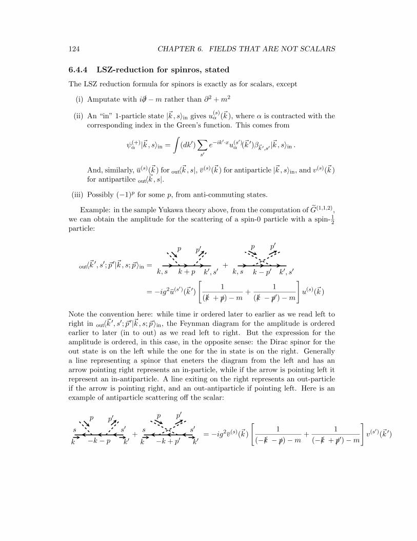
124 CHAPTER 6. FIELDS THAT ARE NOT SCALARS
6.4.4 LSZ-reduction for spinros, stated
The LSZ reduction formula for spinors is exactly as for scalars, except
(i) Amputate with i/∂ −m rather than ∂2 +m2
(ii) An “in” 1-particle state |~k , s〉in gives u(s)α (~k ), where α is contracted with the
corresponding index in the Green’s function. This comes from
ψ(+)α |~k , s〉in =
∫(dk′)
∑s′
e−ik′·xu(s′)
α (~k ′)β~k ′,s′ |~k , s〉in .
And, similarly, u(s)(~k ) for out〈~k , s|, v(s)(~k ) for antiparticle |~k , s〉in, and v(s)(~k )for antipartilce out〈~k , s|.
(iii) Possibly (−1)p for some p, from anti-commuting states.
Example: in the sample Yukawa theory above, from the computation of G(1,1,2),we can obtain the amplitude for the scattering of a spin-0 particle with a spin-1
2particle:
out〈~k ′, s′; ~p ′|~k , s; ~p〉in =k, s k + p k′, s′
p p′
+k, s k − p′ k′, s′
p p′
= −ig2u(s′)(~k ′)
[1
(/k + /p)−m+
1
(/k − /p′)−m
]u(s)(~k )
Note the convention here: while time ir ordered later to earlier as we read left toright in out〈~k ′, s′; ~p ′|~k , s; ~p〉in, the Feynman diagram for the amplitude is orderedearlier to later (in to out) as we read left to right. But the expression for theamplitude is ordered, in this case, in the opposite sense: the Dirac spinor for theout state is on the left while the one for the in state is on the right. Generallya line representing a spinor that eneters the diagram from the left and has anarrow pointing right represents an in-particle, while if the arrow is pointing left itrepresent an in-antiparticle. A line exiting on the right represents an out-particleif the arrow is pointing right, and an out-antiparticle if pointing left. Here is anexample of antiparticle scattering off the scalar:
s
−k − ps′
k k′
p p′
+s
−k + p′s′
k k′
p p′
= −ig2v(s)(~k )
[1
(−/k − /p)−m+
1
(−/k + /p′)−m
]v(s′)(~k ′)

6.5. GENERATORS 125
Note that while the particle and antiparticle scattering amplitudes of the scalarappear superficially different, they are the same (up to a sign) once /ku(~k ) = mu(~k )and /kv(~k ) = −mv(~k ) are used.
Here is an example which involves both u and v spinors: scalar-scalar scatteringinto particle -antiparticle pair (of fermions):
s′
k − ps
k′
k
p′
p
= −ig2u(s)(~k )
[1
(/k − /p)−m
]v(s′)(~k ′)
And, finally, here is an example with a sign from anti-commuting external states,two particles in the initial state scattering into two particles:
2 4
1 3
+
2 3
1 4
= −ig2
[u3u1u4u2
(k1 − k3)2 −M2− u4u1u3u2
(k1 − k4)2 −M2
]
Here we used the compact notation u1 = u(s1)(~k 1), etc. The relative sign betweenthe two terms is a reflection of Dirac statistics of the external states.
6.5 Generators
Let’s study the generators of the Lorentz group in the representation of Weylspinors:
M = 1− i
2ωµνMµν
corresponding to Λµν = ηµν + ωµν with ωµν = −ωνµ infinitesimal. So Mµν are six2×2 matrices that we want to characterize. First we note that det(M) = 1 impliesTr(Mµν) = 0. Next, determine Mµν , using the known transformation propertiesof vectors. On one hand
M †PM = ((Λ−1)µνpν)σµ
= pνσµ(ηµν − ωµν)
and on the other
M †PM = (1 + i2ωµνM
†µν)pλσλ(1− i
2ωσρMσρ)
= pµσµ + i
2ωµνpλ(M†µνσλ − σλMµν) .
126 CHAPTER 6. FIELDS THAT ARE NOT SCALARS
Equating,
i2ωµνpλ(M†µνσλ − σλMµν) = −pνσµωµν = −ωµνpληλνσµ
and since this must hold for arbitrary ωµν and pλ we have
M†µνσλ − σλMµν = −i(ηλµσν − ηλνσµ), .
The solution to this is straightforward:
M0i = −Mi0 = i2σ
i, Mij = −Mji = 12εijkσk,
(Aside: to determine this, expand Mµν in the basis of σµ. Since TrMµν = 0we have Mµν = (aµνj + ibµνj )σj and M†µν = (aµνj − ib
µνj )σj . This gives
aµνj [σj , σλ]− ibµνj σj , σλ = −i(ηλµσν − ηλνσµ) .
Setting λ = 0 gives an equation for the bj ’s:
2bµνj σj = −(δν0σµ − δµ0σν)
and taking µ = 0 and ν = k we have 2b0kj σj = σk from which b0kj = −bk0
j = 12δkj
follows. Similarly we obtain bikj = 0. For the a′s set λ = i. Then
aµνj 2iεjikσk − ibµνj 2δij = −i(ηiµσν − ηiνσµ)
Then setting µ = 0 gives a0νj = 0 and setting µ = l and ν = m gives almj = 1
2εlmj .)
LetJk = 1
2εkijMij = 1
2σk, and Ki =M0i = i
2σi .
Note that J i† = J i while Ki† = −Ki. These satisfy,
[J i, J j ] = iεijkJk, [J i,Kj ] = iεijkKk, [Ki,Kj ] = −iεijkJk .
DefiningJ i± ≡ 1
2(J i ± iKi)
we have[J i+, J
j+] = iεijkJk+, [J i−, J
j−] = iεijkJk−, [J i+, J
j−] = 0 .
You recognize these are two mutually commuting copies of (the algebra of) SO(3) ∼SU(2). You know this from the rotation group in QM: for spinors, ~S = 1
2~σ , and[Si, Sj ] = iεijkSk, while for vectors (Li)jk = −iεijk, with [Li, Lj ] = iεijkLk. Theirreducible representations of SU(2) are ` = 0, 1
2 , 1,32 , . . . of dimension 2` + 1 =
1, 2, 3, 4, . . .. You recognize ` = 0 as a scalar, ` = 12 a spinor, ` = 1 a vector, etc.
Comments:

6.5. GENERATORS 127
(i) For any representation D(Λ) we have infinitesimal generators. If Λµν =ηµν + ωµν then D(Λ)αβ = δαβ − i
2ωµνJµν . The six matrices J µν satisfy the
same commutation relations as Mµν , they are fixed by the multiplication“table” of the Lorentz group, which itself follows form requiring D(Λ) be arepresentation, Eq. (6.2).
(ii) The defining representation is the 4-dim representation acting on vectors,pµ, like Λ itself. That is, D(Λ)µνp
ν = Λµνpν ⇒ − i
2ωλσ(J λσ)µνpν = ωµνp
ν ,from which we read off, for the 4-dimensional (defining) representation of theLorentz group: (J λσ)µν = −i(δλµδσν −δσµδλν ). We can compute easily the same
commutation relations satisfied by the J λσ and of course they are the sameas those satisfied by Mλσ.
(iii) The commutation relations for J i and Ki derived above may seem ambiguoussince they were found from comparing with Pauli matrices but both J i and Ki
are given in terms of Pauli matrices. For example, [Ki,Kj ] = −iεijk 12σ
k waswritten as −iεijkJk rather than −εijkKk. There is a simple argument why[K,K] = −K is excluded. Under parityMij → (−1)2Mij ,M0i → (−1)M0i.Hence J i → J i and Ki → −Ki. This gives, [J, J ] ∼ J but not K, [J,K] ∼ Kbut not J and [K,K] ∼ J but not K.
(iv) We would not have faced this ambiguity (nor would we have had to use theparity argument to sort it out) had we studied the commutation relations forarbitrary representations.
6.5.1 All the representations of the Lorentz Group
Since the same commutation relations must hold for any representation we use thatto construct them. We build on our knowledge of the representations of SU(2).
For J i+ the irreducible representations are classified by s+ = 0, 12 , 1, . . .. The
(2s++1)×(2s++1) matrices are labeled J is+ . For J i− the irreducible representations
are classified by s− = 0, 12 , 1, . . .. The (2s−+1)×(2s−+1) matrices are labeled J is− .
Moreover, since the representation matrices of the generators of the Lorentz group,J i+ and J i−, satisfy [J i+, J
i−] = 0, they are tensor products, J i+ = J is+ ⊗ 1s− , where
1s− is the (2s− + 1) × (2s− + 1) identity, matrix, and, similarly, J i− = 1s+ ⊗ J is− .
The irreducible representation are labeled by (s+, s−) and have generators J i =J i+ + J i− = J is+ ⊗ 1s− + 1s+ ⊗ J is− and similarly for Ki. They have dimension(2s+ + 1)(2s− + 1).
For example, (0, 0) is a representation of dimension 1, a scalar.(1
2 , 0) and (0, 12) have dimension 2. They are spinors. They are two different
spinor representations. Consider (12 , 0):
J is+ = 12σ
i, J is− = 0, ⇒ ~J = ~J + + ~J − = 12~σ ⊗ 1, ~K = 1
i (~J + − ~J −) = − i
2~σ ⊗ 1

128 CHAPTER 6. FIELDS THAT ARE NOT SCALARS
Similarly, for (0, 12)
J is+ = 0, J is− = 12σ
i, ⇒ ~J = ~J + + ~J − = 1⊗ 12~σ ,
~K = 1i (~J + − ~J −) = 1⊗ i
2~σ
But this is where we started from. From ψ′ = Mψ we obtained ~J = 12~σ and
~K = i2~σ so this is the (0, 1
2) representation. So what is (12 , 0)? We already know
that M is a representation. Look more closely:
M = e−i~θ ·( 1
2~σ )−i~γ ·( i
2~σ ) = e−i~α ·(
12~σ ) with ~α = ~θ + i~γ , (αi ∈ C).
The representation we are looking for should have group elements
e−i~θ ·( 1
2~σ )−i~γ ·(− i
2~σ ) = e−i~α
∗·( 12~σ )
whileM∗ = e−i
~θ ·(− 12~σ ∗)+i~γ ·(− i
2~σ ∗) = e−i~α
∗·(− 12~σ ∗) .
This is close. In fact, it is what we want up to a similarity transformation: usingσ2~σ ∗σ2 = −~σ we have
M = σ2M∗σ2 = e−i~α∗·( 1
2~σ ) .
That is, M∗ is in the equivalence class of (12 , 0).
Generalize: note that since M = 1−iωµνMµν we have M∗ = 1−iωµν(−Mµν∗).The matrices −Mµν∗ satisfy the same commutation relations as the Mµν . Moregenrally, if [T a, T b] = ifabcT c then [−T a∗,−T b∗] = ifabc∗(−T c∗), so −T a∗ satisfythe same commutation relations as T a if fabc are real. In our case (J i±) the fabc
are εijk. Since for SU(2) the only irreducible representation of dimension 2s+ 1 isgenerated by ~J s it must be that S(− ~J ∗s)S−1 = ~J s for some invertible matrix S.Now
D(Λ) = e−i~α ·~J +−i~α∗· ~J−
so thatSD∗(Λ)S−1 = e−i~α
∗· ~J +−i~α · ~J−
The role of J+ and J− has been exchanged. To be more precise, the matrix S thatacts on the tensor product exchanges the + and − sectors. We therefore have,
(s+, s−)∗ ∼ (s−, s+)
Note that for s+ = s− the complex conjugate representation is similar to itself.This is a real representation and the vectors on which it acts can be taken to havereal components. For example, let’s investigate the (1
2 ,12) representation. It is 2×2
dimensional. It smells like a 4-vector. Let’s show it is. It is an object with indicesαα as in Vαα, with
V ′αα = M αβMαβVββ
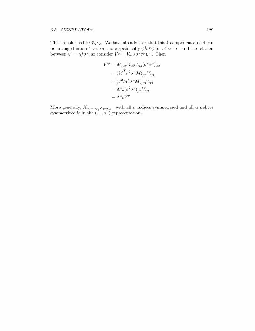
6.5. GENERATORS 129
This transforms like χαψα. We have already seen that this 4-component object canbe arranged into a 4-vector; more specifically ψ†σµψ is a 4-vector and the relationbetween ψ† = χ†σ2, so consider V µ = Vαα(σ2σµ)αα. Then
V ′µ = M αβMαβVββ(σ2σµ)αα
= (MTσ2σµM)ββVββ
= (σ2M †σµM)ββVββ
= Λµν(σ2σν)ββVββ
= ΛµνVν
More generally, Xα1···αs+ α1···αs− with all α indices symmetrized and all α indicessymmetrized is in the (s+, s−) representation.