This file is part of the following reference:

Light, Phillip Richard (1995) The early life history of

coral trout (Plectropomus leopardus) at Green and

Arlington reefs, Australia. PhD thesis, James Cook

University of North Queensland.

Access to this file is available from:

http://researchonline.jcu.edu.au/33778/

If you believe that this work constitutes a copyright infringement, please contact

ResearchOnline@jcu.edu.au and quote

http://researchonline.jcu.edu.au/33778/

ResearchOnline@JCU

THE EARLY LIFE HISTORY OF CORAL TROUT (PLECTROPOMUS LEOPARDUS) AT GREEN

AND ARLINGTON REEFS, AUSTRALIA

by Phillip Richard LIGHT

BSc University of Washington

MSc Florida Atlantic University

A thesis submitted for the degree of Doctor of Philosophy

in the Department of Marine Biology at James Cook University

of North Queensland, in September 1995.

STATEMENT OF ACCESS

I, the undersigned, the author of this thesis, understand that James Cook University of North Queensland will make it available for use within the University Library . and, by microfilm and other means, allow access to users in other approved libraries. All users consulting this thesis will have to sign the following statement:

In consulting this thesis I agree not to copy or closely paraphrase it in whole or in part without the written consent of the author; and to make proper public written acknowledgment for any assistance which I have obtained from it.

Beyond this, I do not wish to place any restrictions on access to this thesis.

1

i ct 1” ( (Date)

STATEMENT OF SOURCES

DECLARATION

I declare that this thesis is my own work and has not been submitted in any form for another degree or diploma at any university or other institution of tertiary education. Information derived from the published or unpublished work of others has been acknowledged in the text and a list of references is given. .

t c't SC,p1,,Afr (Date)

11

in ABSTRACT

The relative contributions of pre- and post-settlement

processes to the early life history of coral trout were examined,

with the aim of understanding how events occurring during

the first year of life influence adult demographic parameters.

Juvenile coral trout showed distinctive patterns of distribution

and abundance at sites around Green Reef, which were

consistent in both space (among sites) and time (between

years). These patterns were influenced by substratum

characteristics, with habitat associations changing as juveniles

grew. Newly settled fish initially showed strong associations

with low-relief, rubble-covered sand bottoms, but switched to

high-relief features such as coral heads and consolidated

rubble mounds after approximately two months of benthic life.

Post-settlement processes (mortality and movement) for new

recruits appeared to be influenced by the amount of sand-

rubble habitat available; individuals occupying areas

containing relatively high amounts of this substratum suffered

less mortality and were more inclined to be site-attached than

those from alternate habitats. Temporal patterns of

recruitment were variable, but a strong settlement event

coincided with the November new moon in all years of the

study.

iv

Following settlement, juveniles were site-attached, and

occupied home ranges that increased in area as they grew.

Home ranges of the smallest recruits (25 - 60 mm SL) showed

little overlap, and this pattern appeared to be facilitated by

intra-specific aggression. Agonistic behaviour was rarely

observed in larger recruits (61 - 102 mm), and home ranges

broadly overlapped.

Recruits displayed an ability to return to former locations

when displaced short distances (20 m), and the distance from

which juveniles could home increased with age. Recruits

displayed higher site-fidelity than 1+ fish; 88% of marked 0+

individuals were resighted within 20 metres of their capture

point, while only 20% of one year old fish were resighted

within these areas.

A change in diet occurred during early growth: diets of newly

settled fish consisted mostly of epibenthic crustaceans,

whereas larger juveniles (60-100 mm) were mainly

piscivorous. Coral trout of all sizes consumed fish, and most

piscine prey were recent recruits to the reef. Foraging modes

and diurnal feeding patterns differed between size classes:

larger juveniles typically fed by ambushing prey (usually

small fish), whereas small recruits concentrated feeding

activities around morning hours, and typically foraged by

striking at invertebrates associated with rubble substrata.

Diets varied spatially for large juveniles, but not for small

individuals: large juveniles inhabiting structurally complex

habitats (coral heads, rubble mounds) shifted to a primarily

piscivorous diet sooner than those from less complex habitats.

Estimates of growth rates of juvenile coral trout were

influenced by larval growth histories, size-selective mortality,

and variations in water temperature. Significant inter- and

intra-annual differences were detected in planktonic growth

rate, which were positively correlated with subsequent benthic

growth. These initial patterns were accentuated by higher

mortality of slow-growing juveniles, which resulted in

relatively faster mean growth rates for juveniles collected later

in the year. Temperature also had a strong influence on

growth, and accounted for 55% of the variability in somatic

growth following settlement.

ACKNOWLEDGMENTS

I have many people to thank for the help and support the y

gave me during this study. First and foremost, I would like to

thank my family for supporting and encouraging me

throughout my university years.

I am also grateful to the numerous volunteers who helped with

field work and made this project an enjoyable one. Martin de

Graaf was one of my first volunteers, and I really appreciated

his enthusiasm and good spirits. Jurgen Mauld was a great

help with netting-making and trout-catching during the second

year. In the third year, I was fortunate to get Nick Currie as an

assistant, and I'll always be thankful for his hard work and

comradery, and also for winning the constant battle to keep the

zodiac from permanently sinking. Many other people

contributed their time and talents to this project. I especially

want to thank Brandon Cole, Brad Cullen, Trish Sposato, the two

Craigs: Humphries and Hutchings, Debbie Currie and Cass Faux,

Mike and Manon Lataveer, and Crystal and Yaniff from France.

Green Island underwent several transformations during the

course of this project, and the transition from a day resort to a

vi

vi i

five star hotel was not without its problems. I want to thank

my fellow light-trap enthusiast, Dave Harris, for keeping the

field station functioning, handling logistical problems, and for

being my occasional unwilling volunteer. Many Green Island

Resort staff members also offered assistance during my stay.

In particular, I thank Alec Taylor for making things run

smoothly and efficiently. The Green Island Dive Shop was a

great help by providing free air fills throughout the project. I

am especially grateful to the Craig family for their help and

friendship, and especially to George, who solved my feeding

problems by letting me scoop baby guppies out of his crocodile

pools. Warren Lelong was a big help in coordinating activities

with D.P.I., providing useful information, and his many efforts

in outfitting the Noel Monkman field station.

Logistic support for this project was primarily supplied by the

Australian Institute of Marine Science, and I have a number of

A.I.M.S personnel to thank for their assistance through the

years. First, I want to thank Mike Cappo for his friendship,

advice, and for sharing his extensive knowledge of fish biology

with me. Tony Fowler also gave me a lot of encouragement

during my first year at A.I.M.S., and taught me some of the

subtleties of otolith work. I also appreciate Dave McKinnon's

help with computer work, and thank Steve Clarke and Karen

Handley for sharing their graphics expertise. Terry Lord

viii

graciously lent me the use of his fence net, and gave me tips on

how to make my own. John Hardman was very helpful in

providing access to marine equipment, and Jeff Warbrick

supplied me with dive gear and maintenance support.

A number of people from James Cook University deserve

special mention for their help with this project. Mark

McCormick was always willing to listen to an idea or answer a

question, and his insight and encouragement are much

appreciated. Julian Caley read and commented on several

manuscripts, and Craig Syms and Natalie Moltschaniwskyj

helped with statistical problems.

The last field season of this project was primarily funded by

the Cooperative Research Centre for Ecologically Sustainable

Development of the GBR (CRC). The Department of Primary

Industries (D. P. I.) was also involved with many aspects of the

project, particularly in allowing me the use of field facilities,

and also in providing personnel to collect juveniles during 1992

and 1993. Portions of the project were funded by the Fishing

Industry Research and Development Council (FIRDEC).

Finally I would like to thank my supervisors for their help

throughout this project. I am grateful for Howard Choat's

support during my candidature, and especially for his help in

obtaining funds for the final year. I thank Peter Doherty for

providing guidance in the initial and final stages of this

ix

research, and also for providing financial and logistic support

during my stays at Green Island and AIMS. Lastly, I thank

Geoff Jones for his many helpful suggestions, critical reviews of

manuscripts, and advice.

TABLE OF CONTENTS

Chapter 1 General introduction 1 1.1 Background 1 1.2 Thesis outline 7

Chapter 2 Recruitment, habitat preferences, ontogenetic habitat shifts in newly settled coral trout (Plectropomus leopardus, Serranidae): are distribution patterns of juveniles influenced by substratum type?

2.1 SYNOPSIS 2.2 INTRODUCTION 2.3 MATERIALS AND METHODS

2.3.1 Study area 2.3.2 Distribution and abundance among sites 2.3.3 Patterns of habitat use among sites 2.3.4 Patterns of habitat use by 0+ fish within the Primary site 17 2.3.5 Timing of recruitment 21 2.3.6 Changes in density 22 2.3.7 Effect of sampling scale on measurement of habitat selection 22 2.4 RESULTS 25 2.4.1 Distribution and abundance among sites 25 2.4.2 Patterns of habitat use among sites 29 2.4.3 Patterns of habitat use within a site 30 2.4.4 Timing of recruitment 31 2.4.5 Changes in density 32 2.4.6 Effect of sampling scale on measurement of habitat selection 34 2.5 DISCUSSION 37

Chapter 3 Movement patterns, home range, and homing behaviour in juvenile coral trout

3.1 SYNOPSIS 3.2 INTRODUCTION 3.3 MATERIALS AND METHODS

3.3.1 Study site 3.3.2 Marking of juveniles 3.3.3 Calculation of home ranges 3.3.4 Parameters of the home range 3.3.5 Home range of 1+ fish. 3.3.6 Persistence 3.3.7 Homing 3.3.9 Behavioural observations

3.4 RESULTS 3.4.1 Effects of branding

10 10 11 15 15 16 17

49 49 50 53 53 53

54 55 57 58 59 60 62 62

Xi

3.4.2 Home range 62 3.4.3 Persistence 3.4.4 Homing 65 3.4.5 Home range overlap between neighboring fish 67 3.4.6 Behaviour 68

3.5 DISCUSSION 71

Chapter 4 Spatial and ontogenetic variation in the feeding biology of juvenile coral trout, Plectropomus leopardus 82

4.1 SYNOPSIS 82 4.2 INTRODUCTION 83 4.3 MATERIALS AND METHODS 84

4.3.1 Behavioural observations 85 4.3.2 Specimen collection 87 4.3.3 Stomach content analysis 88

4.4 RESULTS 90 4.4.1 Behavioural patterns 90 4.4.2 Stomach fullness/digestive state 92 4.4.3 Stomach contents 93 4.4.4 Variations in diet between size classes 95 4.4.5 Variations in diet between habitats 96 4.4.6 Comparison between regurgitated prey and stomach contents 98

4.5 DISCUSSION 98

Chapter 5 The influence of size at settlement, temperature, and size-selective predation on variations in growth rate in juvenile coral trout 106

5.1 SYNOPSIS 106 5.2 INTRODUCTION 107 5.3 MATERIALS AND METHODS 110

5.3.1 Sample collection and sites 110 5.3.2 Water temperature 1 1 2 5.3.3 Otolith preparation and measurement 1 1 2 5.3.4 Otolith growth : somatic growth correspondence 1 1 4 5.3.5 Spatial and temporal patterns of growth inferred from increment widths 1 1 5 5.3.6 Effect of water temperature on somatic growth rate. 1 1 6 5.3.7 Back-calculation of size at settlement and pre- settlement growth rate inferred from increment widths 1 1 7 5.3.8 Overall growth rates 1 1 8

Length at age estimates 1 1 8 Direct measurement 1 1 8 Modal progression analysis 1 1 9

5.3.9 Intra-annual growth variation among cohorts 1 1 9 5.3.10 Data analysis 12 0

5.4 RESULTS 1 2 1

5.4.1 Relationship between otolith growth and somatic growth 1 21

5.4.2 Spatial and temporal patterns of growth inferred from increment widths 1 21 5.4.3 Post-settlement growth rates calculated from increment widths 1 2 4 5.4.4 Pre-settlement increment widths 12 5 5.4.5 Size at settlement and pre-settlement growth rate 1 2 5 5.4.6 Effect of water temperature on somatic growth rate. . . 1 27 5.4.7 Variation in standard length between reefs, years, and seasons 1 2 7 5.4.8 Overall growth 1 2 8

Length at age estimates 1 2 8 Otolith length / fish length correspondence 1 3 2 Direct measurement of growth 1 3 3

5.4.9 Intra-annual growth variation among cohorts 1 3 3 5.5 DISCUSSION 134

Chapter 6 GENERAL DISCUSSION 1 40

6.1 Major findings 1 40

6.2 Conclusions 146

Bibliography 1 48

x i i

CHAPTER 1

GENERAL INTRODUCTION

1.1 Background

Recruitment of larval fishes to coral reef habitats is a brief

demographic event, which precedes a relatively long period of

benthic life (Jones 1990). Although the influence of

recruitment variation on population structure is well

documented (Doherty 1983, Victor 1983), attention has

recently been focussed on the numerous ways in which

patterns established at the time of settlement may be modified

(Jones 1987, 1991).

The increasing interest in post-recruitment processes is

driven in part by a number of studies reporting poor

correlations between recruitment history and adult population

numbers at the patch reef scale (Robertson 1988, Jones 1987,

Forrester 1990, but see Doherty and Fowler, 1994). For

example, Robertson (1988) found that abundances of adult

surgeonfish were not correlated with settlement patterns over

a six year period. He attributed these differences to relocation

between habitats, and noted that relocation may be the norm

in species for which recruits, juveniles, and adults occupy

different habitats. Distribution patterns can be expected to be

influenced by post-settlement habitat selection and

redistribution in highly mobile species (Brock et al. 1979, Jones

1991), or those having different habitat requirements during

growth (Choat and Bellwood 1985). However, the contribution

of post-settlement dispersal to changes in abundance have

rarely been measured for coral reef fishes (Doherty 1982,

1983, Jones 1987, 1988, 1991).

To date, most studies have investigated these processes as

they pertain to highly sedentary species such as pomacentrids,

and have used small coral reef patches as replicate units. This

is because juvenile pomacentrids are relatively abundant,

conspicuous, and easily monitored. However, pomacentrids are

characterised by specific life history features that influence

their settlement patterns and post-settlement processes.

Newly settled individuals are large relative to adult size

(Wellington and Victor 1989), and as a result they tend to

recruit directly into adult habitats from which they rarely

move during their lives (Doherty 1983, Williams 1991). Thus,

extrapolation of results from studies involving this family may

lead to erroneous conclusions when applied to species with

different characteristics.

Coral trout, Plectropomus leopardus, are high-level carnivores

and the most valuable food fish exploited on the Great Barrier

Reef (Williams and Russ 1991). Their large size, elevated

position in the food chain, and high mobility as adults make

them an interesting contrast to the sedentary pomacentrids

upon which most studies of juvenile reef fish ecology have

2

been based. As with most groupers (Richards 1990), much of

the early life history is unknown (Leis 1987), due mainly to the

cryptic behaviour and relative rarity of the juveniles.

Moreover, young serranids often occupy heterogeneous

habitats which are not easily sampled by conventional

techniques (Ross and Moser 1995). As a result of these

difficulties, a large gap exists in our knowledge of grouper

ecology.

Although previous studies of coral trout have concentrated on

the adult phase (Goeden 1978, Ayling 1991, Kingsford 1992,

Ferreira 1994, Davies 1995), the relatively site-attached

behaviour of newly settled individuals makes them

particularly amenable to the use of mark-recapture techniques

for studying movement and growth. Furthermore, fluctuations

in abundances of pre-settlement coral trout have been shown

to vary with lunar period (Doherty et al. 1994) which may

result in the presence of multiple cohorts within a settlement

season. These features of the early life history of coral trout

make them ideal subjects for intra-specific comparisons of

growth, behaviour, and movement.

Demographic parameters of coral reef fish populations are

influenced by processes occurring during both planktonic and

benthic phases of the life cycle (Sale 1985, Jones 1987,

Richards and Lindeman, 1987, Jones 1991). For the past

decade, research into the factors affecting reef fish

3

demography has been influenced by the "recruitment-

limitation" hypothesis, which proposes that coral reef fish

populations are maintained at levels below numbers set by

available resources (Doherty 1983, Victor 1983). Based on

this hypothesis, numbers of fish recruiting to reefs will be

determined by processes occurring within the plankton, and

variations in adult populations will reflect numbers of

individuals recruiting to benthic habitats. This model draws

strong support from studies of widespread natural

disturbances such as El Nino events and Acanthaster outbreaks,

in which increases in algal food supply have failed to produce

corresponding increases in herbivore populations (Doherty

1991) .

In contrast, the "resource-limitation" hypothesis (Smith and

Tyler 1972, Shulman 1984, Hixon and Beets 1989) proposes

that populations are regulated at or around a carrying capacity

by competition for limited resources - mainly shelter.

According to this model, density-dependent processes should

control levels of settlement, growth, and survival of reef fishes.

Studies testing these alternate hypotheses have generally

concluded that they are extremes in a continuum, and that the

limitation of populations by planktonic processes or density

dependent post-settlement processes is largely a matter of

degree (Forrester 1990, Jones 1990). Furthermore, whether

4

reef fish populations are limited by recruitment or resources

may vary between species, or within species in different

locations (Williams 1980, Hunte and Cote 1989).

Although considerable progress has been made in

documenting numerical aspects of recruitment, little attention

has been focussed on qualitative aspects of individuals at the

time of settlement. For example, the extent to which variations

in body size at settlement biases probabilities of future

survival or how such effects are transferred to adult growth

have seldom been addressed. These variations may play an

important role in predicting demographic parameters of adult

populations, because relatively small changes in the previous

larval growth rates may result in large variations in the

numbers surviving to settlement (Houde 1987, Miller et al.

1988, Pepin and Meyers 1991).

While individuals often differ in size at settlement, their

habitat requirements at this time may be quite specific (Sale et

al. 1984, Eckert 1985), and these choices may have important

consequences for post-settlement ecology. Strong habitat

selection often leads to higher densities within settlement

areas, with possible compensatory effects on growth (Jones

1987, Forrester 1990). In addition, size-selective predation on

smaller size classes is common (Post and Evans 1989), and

consequently spatial variability in the availability of suitable

shelter may be important in determining predation levels for

young fish (Eckert 1985, Aldenhoven 1986, Jones 1988). For

5

example, Shulman (1984) found that settlement and/or post-

settlement survival for several families of coral reef fishes

(Gobiidae, Pomacentridae, Acanthuridae, Haemulidae) were

strongly limited by access to shelter sites. Since availability of

shelter and rate of growth are both considered to be major

determinants of early juvenile survivorship, newly settled fish

may be expected to exhibit behaviour that minimises the risk

of predation while maximising growth (Tupper and Boutilier

1995).

The present study examines how demographic parameters of

juvenile coral trout are affected by pre- and post-recruitment

processes. The principal aim is to assess the relative

contributions of these processes to distributions and

abundances of juveniles during ontogeny. Specifically, this

study describes aspects of the early life history of coral trout

from the planktonic stage until entry into the adult population,

with particular emphasis on the first several months after

settlement. Changes in habitat use, movement patterns,

feeding biology, and growth are considered in relation to

observed patterns of distribution and abundances.

Recruitment patterns are examined, in order to address

questions about the timing of recruitment and differences in

growth between monthly cohorts. Finally, the influence of

larval growth histories on subsequent post-settlement growth

is discussed.

6

This is the first study to examine juvenile demographic

factors for a tropical serranid. A growing body of evidence

suggests that the first months of benthic life represents a

critical "bottleneck" in fish ecology (Werner and Gilliam 1984),

during which selective pressure to grow rapidly through

vulnerable size classes may be extreme (Post and Prankevicius

1987). By examining changes in habitat preferences,

movement, diet, and growth that occur during coral trout

ontogeny, the present study identifies these as more than a

group of unrelated events, but rather as a suite of

simultaneous changes which reflect a major ecological

transition in juvenile coral trout.

1.2 THESIS OUTLINE

CHAPTER 2: Recruitment, habitat preferences, and

ontogenetic habitat shifts in newly settled coral trout,

(Plectropomus leopardus, Serranidae)

The densities of newly settled coral trout and their associated

habitats are examined at sites around Green Reef. Specific

micro-habitat preferences of newly settled fish are assessed.

Observations of marked individuals over time are used to

determine if juveniles shift to different habitats as they grow.

Temporal patterns in recruitment are evaluated using back-

calculated settlement dates. Changes in density are monitored

7

8

over a two month period at two sites. Possible causes of

observed habitat-use patterns are discussed.

Chapter 3: Home range, homing behaviour, and

activity patterns of juvenile coral trout Plectropomus

leopardus.

Observations of marked individuals are used to describe space

use patterns of newly settled and older juveniles. Two

experiments are described which measured the tendency of

juveniles to return to original areas after displacement.

Behavioural observations are used to examine the influence of

size-specific changes in agonistic behaviour in regulating

spacing of individuals. Parameters of the home range are

described and used to interpret behavioural data. The

importance of home range behaviour for influencing local

juvenile density is discussed.

Chapter 4: Spatial and ontogenetic variation in the

feeding ecology of juvenile coral trout.

Ontogenetic and spatial variation in diet and feeding biology of

juvenile coral trout are examined, with particular emphasis on

the implications of a shift towards piscivory. Behavioural

observations are used to examine diurnal patterns in feeding

behaviour. Foraging styles employed by juveniles are

described. The use of samples of regurgitated prey items to

9

estimate total gut content is evaluated. The role of habitat

shifts in fostering size-specific asymmetries in feeding ecology

is discussed, followed by a discussion of the impact of juvenile

coral trout piscivory on the demography of coral reef fish

populations.

Chapter 5: The influence of size at settlement,

temperature, and size-selective predation on

variations in growth rate in juvenile coral trout.

Spatial and temporal variation in growth rates are assessed,

using three independent methods of estimation. Daily

increment deposition and the correspondence between otolith

growth and somatic growth is validated using tetracycline

marked field specimens. The influence of seasonal

temperature change is evaluated, using instantaneous growth

estimates back-calculated from increment widths. Changes in

growth parameters are assessed by comparing growth rates of

populations collected shortly after settlement with those from

later collections. Larval growth histories are compared to

subsequent post-settlement growth to determine whether size

at settlement and pre-settlement growth determine growth

and success during benthic life.

Chapter 6: General Discussion

Chapter 2

RECRUITMENT, HABITAT PREFERENCES, AND

ONTOGENETIC HABITAT SHIFTS IN NEWLY SETTLED

CORAL TROUT, (PLECTROPOMUS LEOPARDUS,

SERRANIDAE)

2.1 Synopsis

The densities of newly settled coral trout (Plectropomus

1 eopardu s) and their associated habitats were monitored on

Green Reef to assess the extent to which habitat selection and

post-settlement habitat shifts influence the distributions of

juveniles. Surveys showed that small juveniles did not

randomly select settlement sites and that these habitat

associations changed as they grew larger. Specifically, coral

trout recruited to level patches of rubble substrata > 5 m2 in

area and subsequently shifted to high relief features in the

environment. Densities of recruits were related to the amount

of rubble substrata available at sites. Loss of individuals from

areas was related to density anfd the amount of available

shelter. It is hypothesised that initial preferences for these

substrata are due to predator avoidance strategies of newly

settled fish, and that subsequent habitat shifts are a

consequence of changes in the size of refugia required by

growing fish.

1 0

2.2 Introduction

A significant component of the distribution and abundance of

coral reef fish can be explained by spatial heterogeneity within

the environment (Smith and Tyler 1972, Luckhurst and

Luckhurst 1978, Bell and Galzin 1984). In particular, newly

settled reef fish often have restricted depth distributions and

are associated with specific habitats (Ehrlich 1975, Sale 1980,

Sale et al. 1980, Williams 1980, Doherty 1983, Eckert 1985).

One explanation for these patterns is that larval fish possess

precise habitat requirements at settlement and actively select

these sites (Sale et al. 1980).

Settlement sites selected by reef fish are known for only a

few species (Leis 1991). Although numerous field studies have

demonstrated apparent selection by juvenile damselfishes

(Williams 1980, Sweatman 1988), and other reef-associated

species (Sale et al. 1984, Eckert 1985), less is known about the

habitat preferences of the juveniles of large, carnivorous fish.

In particular, little research has been devoted to the early life

stages of serranids (Leis 1986, Richards 1990), primarily

because they tend to be cryptic and rare. If newly settled

serranids do preferentially associate with specific habitats,

information about the characteristics of the preferred

substratum could have important implications for the

management of this important commercial resource (Keener et

al. 1988).

11

The period following settlement to these habitats is extremely

important to the subsequent ecology of reef fish. For example,

mortality of a fish cohort has been estimated to be as high as

99% in the first 100 days of life (Cushing 1974). Leis (1991)

described the rapid behavioural and morphological changes

required by settlement-stage fish during the critical transition

from pelagic to reef environments, and emphasised the

vulnerability of these potential recruits. Vulnerability to

predation usually decreases with size (Jones and Johnston

1977), hence selection may favour rapid growth during this

period. Furthermore, to the extent that predation pressure on

early stages restricts individuals to particular habitats, local

competition for resources may increase - the "recruitment

bottleneck" phenomena (Neill 1975). Under these

circumstances, it may be advantageous for an individual to

switch to an alternate habitat as quickly as possible. Such

ontogenetic shifts are not uncommon in fish, particularly in

species that attain large sizes (Werner and Gilliam 1984).

Coral trout, Plectropomus leopardus, (Lacepede) are top

carnivores and the most valuable food fish on the Great Barrier

Reef (Williams and Russ 1991). With few exceptions, previous

studies of this fish have concentrated on the adult phase and

have considered differences in density at whole-reef scales.

Ayling et al. (1991) monitored the abundances of both juvenile

and larger coral trout in front and back reef habitats on 26

12

reefs in the Cairns section of the Great Barrier Reef. They

reported variation in the numbers of coral trout recruiting to

each habitat, but attributed this to differential removal of

cannibalistic adult coral trout, as a result of fishing activities.

More recently, Doherty et al. (1994) used light traps to collect

pre-settlement coral trout from sites in the same region. In

addition to reporting strong lunar periodicity in the

abundances of coral trout larvae, they also found that catches

were higher at certain sites, indicating that recruitment levels

to benthic habitats beneath these sites may also be high.

This information suggests that densities of newly settled coral

trout may vary spatially, and raises the possibility that

differential mortality rates may exist between locations as a

result of density-dependent processes (e.g. competition for

food, suitable shelter). Although information concerning

mortality is notoriously difficult to obtain, such data is likely to

be of major importance in interpreting the dynamics of fish

populations (Jones 1991). The limited information available

suggests that there is often considerable intra-specific

variability in mortality rates at small spatial scales

(Aldenhoven 1986, Victor 1986, Mapstone 1988). To date,

studies reporting density-dependent mortality have usually

examined this process using small units of habitat such as

mollusc shells or concrete blocks (Shulman 1985, Hixon and

Beets1989). Mortality studies examining variability at within-

reef scales are comparatively few, but are essential to

13

identifying variation in abundances among physiographic

habitat zones of individual reefs.

The importance of selecting an appropriate sampling scale

with which to measure patterns and processes has been

emphasised by Ogden and Ebersole (1981). Measurement of

patterns of habitat use and recruitment for highly mobile fish

such as coral trout may be complicated because they may

dramatically increase their range of movements during

ontogeny (Davies 1995). Consequently, habitat selection at

settlement may be manifest over relatively small distances,

reflecting the scales at which larval fish respond to differences

in the environment. On the other hand, a sampling scale of

hundreds of metres may be necessary to detect changes in the

fish-habitat associations of older juveniles resulting from

coarse-grained variation in reef morphology. Therefore,

several sampling scales may be needed to measure changes in

habitat use during ontogeny.

The objectives of this study were:

to identify temporal and spatial patterns in coral trout

recruitment at Green and Arlington Reefs.

to determine if specific sites are occupied by juvenile coral

trout at the time of settlement.

to establish whether shifts in habitat use occur during

growth.

14

4) to assess the importance of shelter availability and recruit

density in influencing post-settlement processes.

2.3 Materials and methods

2.3.1 Study area

The study was conducted at Green Reef, in the Cairns Section

of the central Great Barrier Reef Marine Park (Fig. 2.1),

between January 1992 and February 1995. Four sites (Si - S4)

were chosen around the periphery of the reef, in depths

ranging between 8 - 15 metres (m). Sites were selected in

conjunction with another study (Doherty et al. 1994) which

identified the presence of pre-settlement coral trout at these

locations. Si was designated the "Primary Area" and was used

to make detailed observations on newly settled fish. Within

the Primary Area, two sections measuring 50 x 50 m (Site A),

and 40 x 100 m (Site B) were gridded and mapped in order to

monitor recruitment, densities, and habitat associations of

newly settled coral trout. The difference in grid size was

necessary due to the configuration of habitats: sand-rubble

patches were generally bordered by undulating consolidated

rubble mounds. Thus, to ensure that grids compared

reasonably similar sections of substrata, dimensions were

selected which matched topography.

15

16 2.3.2 Distribution and abundance among sites

Timed swims were used to assess the abundance of juveniles

at each of the four sites. Each survey consisted of nine

replicate 20 minute swims per site, covering a total area of

approximately 1500 m2 . Replicates were separated by a short

interval (3 - 5 minutes), during which divers were transported

by boat to another haphazardly selected starting point. Visual

landmarks were noted during each replicate, to insure that the

same area was not censused twice during a survey. A zig-zag

course was followed, in order to include as many habitat types

and depths as possible. One observer (PRL) methodically

searched all habitats for the presence of juveniles. Standard

lengths for all fish < 200 mm were estimated, and the

associated habitat recorded. Sites were surveyed in December

1993 and 1994, and January 1994 and 1995. Two size classes

were used in this study: 25 - 105 millimetres (mm), and 140 -

200 mm standard length (SL). The latter size class contained

few individuals at the lower end of the range, and no juveniles

in the 105 - 140 mm range were seen during the sampling

period. As a result of this bi-modal distribution, and based on

otolith studies, (Chapter 5) these, size classes were considered

to represent 0+ and 1+ cohorts. The accuracy of size estimates

was checked during a concurrent study by capturing and

measuring fish following length estimation; estimates were

within 5 mm of actual size for 0+ fish, and within 10 mm of

actual size for 1+ fish.

- 1 6°4 5.

410 III oletty ' • :. .

0 1

2KM I I I

I I 1 6°4 5' --

Ell

Site B SR site

CRM site

Site A

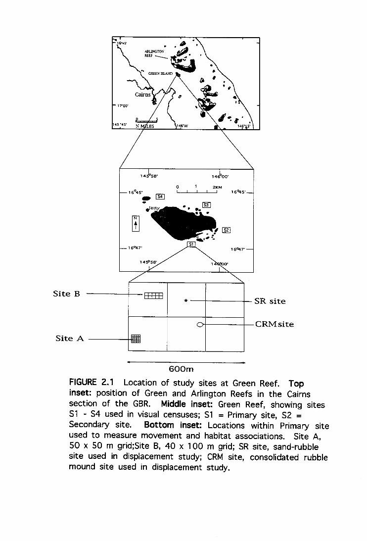
600m FIGURE 2.1 Location of study sites at Green Reef. Top inset: position of Green and Arlington Reefs in the Cairns section of the GBR. Middle inset: Green Reef, showing sites S1 - S4 used in visual censuses; S1 = Primary site, S2 = Secondary site. Bottom inset: Locations within Primary site used to measure movement and habitat associations. Site A, 50 x 50 m grid;Site B, 40 x 100 m grid; SR site, sand-rubble site used in displacement study; CRM site, consolidated rubble mound site used in displacement study.

17

2.3.3 Patterns of habitat use among sites

Point - intercept line transects were used to estimate percent

habitat cover at each of the sites. Optimal sample size (transect

lengths and number of sample points) was determined during

a pilot study, by comparing estimates of substrate cover with

previously determined values. Consequently, five replicate 50

m transects were placed haphazardly over the substratum.,

and 8 random points were selected along each transect. The

substratum directly below each point was classified into one of

four habitats: sand, rubble, live coral, and algae. The resulting

40 random points were used to determine mean (± se)

frequency of cover for each of the categories.

2.3.4 Patterns of habitat use by 0+ fish within the

primary site

In order to quantify habitat associations of newly settled fish

and to determine their positions relative to prominent features

in the environment, a 50 x 50 m section within the primary

area (Site A) was selected which contained relatively high

numbers of recruits and offered a wide range of potential

habitats. This section was subdivided into 10 x 10 m squares,

and all features within each square (i.e. coral heads, rubble

mounds, patches of macro algae, dead coral) were mapped with

a resolution of approximately 50 centimetres (cm) and

transferred to an X-Y coordinate system. Daily censuses were

conducted using SCUBA between 8 December 1993 and 6

February 1994. These consisted of an observer (PRL) swimming up and down the grids while thoroughly inspecting

the bottom, and recording the position and identity of each

marked fish on an underwater map. Individuals were

recorded only once per day. A 30 m strip immediately outside

the perimeter of the mapped area was also searched, to census

fish which had ranged outside the grid. Censuses required

about 45 minutes to complete, and were conducted at

randomly selected times of day to minimise the effects of

diurnal behaviour patterns.

Habitat was quantified using six replicate point-intercept

transects. The resulting 48 points were assigned to the four

habitat categories described above, except that rubble habitats

were further subdivided into sand-rubble, rubble mounds, and

dead coral to allow for finer partitioning of the environment

(Table 2.1). Depth was 10 - 11 m. at high tide.

18

Table 2.1. Habitat types used in use/availability study, and descriptions.

HABITAT DESCRIPTION SAND/RUB BLE

Level expanses of sand bottom, covered with medium-grade rubble, <10 cm along major axis.

RUBBLE MOUNDS

Large (>10m2) piles of consolidated dead branching coral, often covered with macroalgae, (Sargassum, Caulerpa) rising to 5 m above bottom.

LIVE CORAL

hard and soft corals

ALGAE benthic macroalgae, 5 - 15 cm in height

SAND uniform patches of sand containing little or no rubble

DEAD CORAL

rocks > 0.5 m

0+ fish were divided into two size classes: 25 - 60 mm, and 61

- 105 mm. Members of the first size class were designated

"small recruits" and the latter were considered "large recruits".

In order to identify individuals, selected fish were marked

and released. Fence nets were used to capture these juveniles

(n = 57), and they were branded with individual marks using a

12 volt soldering tool located on the boat. The branding

procedure involved placing the fish on a board with its head

covered by a moist towel, and lightly touching the shank of the

heating element to the body. This technique cauterised the

19

skin, and produced a white line approximately 0.5 cm wide,

which changed to dark gray after 2 - 3 weeks Although the

marks became more difficult to recognise after the colour

change they were still visible for two months. Individuals

were recognised by different combinations of brand position

(left side, middle etc.) and orientation (/, -, <, >, etc.). After

branding and measurement, each fish was returned to the

exact point of capture, usually within 10 minutes.

Observations of branded fish in captivity and in the field

indicated that fish were not adversely affected by the

procedure (aquaria fish readily consumed prey within an hour

of marking, and released individuals were observed to forage

and interact with con- and hetero-specifics on the following

day).

Daily positions of marked fish were recorded on an

underwater map, and the most divergent observation points

for each individual were connected to estimate home range.

Subsequent plots of the area of these convex polygons and the

number of resightings showed that home range was estimated

reasonably with a minimum of twelve resightings (Chapter 3).

Consequently, the areas of fish with twelve or more resightings

were used to indicate their positions relative to spatial

reference points inside the grid.

The null hypothesis that juvenile coral trout use habitats in

proportion to their availability was evaluated using two tests.

20

First, resightings of all marked recruits were pooled and

divided into the two size classes. Frequency distributions of

the number of fish seen on habitats were compared to habitat

availability, using Chi-square tests.

As a second test of habitat selection, the Linear Resource

Selection Index (Strauss 1979) was used to estimate habitat

selection of individual fish:

L = ri - pi,

where L is the measure of preference, ri = relative utilisation of

substratum i (i. e. number of associations of one individual

with substratum i divided by the total number of resightings of

that individual), and pi = overall proportion availability of

substratum i. Expected values of this index fall between ±1 ,

with zero indicating random association, positive indicating

selection of a substratum, and negative values indicating

avoidance of the substratum. Selection indices were calculated

for all fish resighted 12 or more times, and the means of new

and large recruits were compared using Student's t-test. T-

tests were also used to assess whether values were

significantly different from zero for each habitat (a = 0.05)

(Morrissey and Gruber 1993).

2.3.5 Timing of recruitment

Juvenile coral trout were collected from Green Reef from 1992

- 1995 for use in an otolith-based study of recruitment and

21

growth (Table 5.1); additional individuals were collected from

Arlington Reef during 1992 to assess variation in recruitment

between reefs. Sagittae were removed from juveniles, cleaned,

weighed and measured. Sagittae from individuals collected in

1992 were prepared and analysed by personnel from the

Central Ageing Facility (CAF) in Victoria, and lapilli from the

same individuals were used to determine pre-settlement age

(Chapter 5). Back-calculated settlement dates were

determined for each fish by subtracting total age minus mean

pre-settlement age from collection dates. Age and sagittae

length were strongly correlated; consequently, this relationship

was used to back-calculate settlement dates for juveniles

collected during the final two years of the study (Chapter 5).

2.3.6 Changes in density

Density of newly settled individuals were monitored during

weekly censuses of both Site A and Site B, between 8 December

1993 and 29 January 1994; Site B was not censused during the

first week of this period. New recruits were collected, marked,

and returned to the point of capture during each weekly

census. Grids were thoroughly inspected during censuses; thus,

it was assumed that all individuals present were captured and

marked. The number of marked recruits were compared to the

number from the previous week, and the percent missing from

grids was considered the disappearance rate (losses due

mortality and/or relocation). Recruitment rates were estimated

22

from the numbers of unmarked individuals (new recruits)

recorded on the grids each week.

2.3.7 Effect of sampling scale on measurement of

habitat selection

To determine the spatial scale at which settlement sites

differed from randomly chosen sites, 33 recruits (mean SL 36.7

± 1.2 mm, range 25 - 47 mm) were captured and measured

during 1994 - 1995. For each fish located, the surrounding

habitat was quantified at three spatial scales using quadrats of

nested size (1, 2, and 5 m squared). The quadrat was centred

on the position where the fish was first sighted and the

surrounding habitat was classified under each of 36 evenly-

spaced points into one of 11 habitat categories. These habitat

categories were defined as: (1) Rubble - bits of dead coral < 10

cm. (2) Sand - fine grained calcareous sediment. (3) Algae -

macro algae (e. g. Halimeda, Sargassum, Caulerpa). (4) Rock -

dead coral > 10 cm, firmly embedded in substratum. (5) Live

branching coral - (e. g. Acropora, Pocillopora). (6) Live massive

coral - (e. g. Porites, Goniopora). (7) Live plate coral - (e. g.

Agariciidae). (8) Sponge. (9) Soft coral. (10) Consolidated

rubble - mounds of dead branching coral, rising 4 - 8 m above

the sea-bed. (11) Consolidated algae/rubble - similar to (10)

but encrusted with turf and/or calcareous algae.

23

To provide a valid comparison, null sites were selected using

a compass and sets of two random numbers. The first random

number in a set (integer between 1 and 8 inclusive) specified

the compass quadrat (to the nearest 45 degrees); the second (0

- 99 inclusive) determined the number of fin strokes to swim

from the point of origin. Once the null position was

determined, the surrounding habitat was quantified by the

same procedures using the same three nested quadrats. The

points underlying the quadrats were recorded as above.

Chi-square tests on total frequency counts for each of the 11

habitat groups were used to assess whether habitats selected

by recruits differed from null sites. In order to assess whether

patterns of habitat use differed between spatial scales,

principal component analysis (PCA) was used to reduce the

data set to a smaller number of uncorrelated components. The

characteristics of the sites selected by the 33 fish were

analysed at each scale separately, and for all three scales

combined. Principal component axes (PCs) were characterised

by their correlations with the original microhabitats:

correlations were considered significant if they had an absolute

magnitude greater than 0.5 (Paulissen 1988). Microhabitats

selected by recruits were expressed as a subset of all

microhabitats potentially available at each scale. Means and

standard errors of eigenvalues along each PC axis were

calculated, and significant differences between selected and

random scores were identified at each of the three scales and

24

for all scales combined, using Student's t-test (a

0.05)(Paulissen 1988).

=

2.4 Results

2.4.1 Distribution and abundance among sites

The pattern of distribution of recruits among sites at Green

Island was relatively consistent between years (Fig. 2.2). 51

and S2 received the highest number of 0+ fish in both years

sampled, but the overall magnitude was higher in the second

year. When counts from both seasons were combined, 63

recruits were recorded from Si and S2 compared to only three

from other sites.

As with 0+ fish, total numbers of 1+ fish recorded during the

study were greatest at Si and S2. However, site by site

comparison of the distributions of 0+ fish from the first season

with distributions of 1+ fish from the second year, shows that

despite a lack of recruits at S3 in 1993 - 1994, 1+ fish were

present at this site during the following season, at densities

equivalent to Si and S2.

Analysis of variance of 0+ fish counts using years, months,

and sites as fixed factors and number of fish seen per 20

minute swim as the response variable, detected a significant

interaction between year and site (Table 2.2), suggesting that

25

DECEMBER '94

ill aTrx1 I II 1 2 3 4

SITE

NU

MB

ER

OF JU

VEN

ILES

PER

20

MIN

. SW

IM

3-

2—

1111•1••••

0

3 -

2—

1-

0

DECEMBER'93

JANUARY '94

1

2

4

1

2 3 4 SITE

SITE

Fig. 2.2. Mean (± SE) number of juveniles seen per 20 minute swim at sites around Green Reef (n = 9 swims per site). Dark bars: 0+ fish, Light bars: 1+ fish.

26 the magnitude of recruitment to individual sites varied between years . Multiple comparisons revealed higher

abundances in 1994 - 1995, and for censuses in January.

Recruitment at Si was significantly higher than at other sites

(Tukey's test, a = 0.05).

Counts of 1+ fish were also higher in 1994 - 1995. A significant interaction was found between year and month

(Table 2.3), indicating that the trend in the distribution pattern

differed from that of 0+ fish. Multiple comparisons indicated a

more even distribution of 1+ fish relative to recruits: there

were no significant differences between abundances at Si, S2,

and S3, and fish counts between months did not differ

significantly.

Table 2.2. Table 2.3. (A) ANOVA of no. of 0+ fish seen per 20 min. swim. (B) Tukey's test of no. of juveniles seen per 20

min. swim. Treatment levels not significantly different at the

0.05 level share an underline. Treatment levels are arranged

in increasing order of juvenile abundance.

A. Source df MS F P

Year 1 11.67 57.97 <0.0001

Month 1 2.51 12.45 <0.001

Site 3 9.56 47.48 <0.0001

Year x Month 1 0.17 0.86 0.36

Year x Site 3 5.82 28.91 <0.0001

Month x Site 3 0.40 1.97 0.12

Yr x Mo x Site 3 0.06 0.31 0.82

Residual 128 0.20

B. Main effect

Year 1993-1994 1994-1995 Month December Januar Site S4 S3 S2 S1

27

Table 2.3. (A) ANOVA of no. of 1+ fish seen/20 min. swim.

( B ) Tukey's test of no. of juveniles seen/20 min. swim.

Treatment levels not significantly different at the 0.05 level

share an underline. Treatment levels are arranged in

increasing order of juvenile abundance.

A. Source df MS F P

Year 1 9.0 17.34 <0.0001

Month 1 0.25 0.48 0.49

Site 3 3.72 7.17 <0.005

Yr x Mo 1 2.25 4.33 <0.05

Yr x Site 1 0.80 1.53 0.21

Mo x Site 3 0.82 1.59 0.20

Yr x Mo x Site 3 2.0 1.8 0.20

Residual 128 0.52

B. Main effect

28

year

month December January

site S4

S3 S2 SI

1993-1994 1994-1995

2.4.2 Patterns of habitat use among sites

Analysis of transect data detected significant between-site

differences in frequency of occurrence of rubble, sand, algae,

and live coral (Table 2.4). Si had the highest proportion of

rubble substrata, while S4 had relatively high amounts of coral.

S2 had the highest component of algae. Comparison of mean

abundance of 0+ and 1+ fish with mean frequency of rubble

cover at each site (Fig. 2.3) indicated a positive correlation for

0+ fish, (Spearman's Rank Correlation Coefficient, rs = 1.0, n = 4,

p < 0.05), but not for 1+ fish (rs = 0.6, n = 4, p > 0.05).

TABLE 2.4. (A) One way ANOVA of habitat cover at four

sites around Green Reef, based on forty random points per site.

(B) Tukey's test of frequency of habitat at each site. Sites not

significantly different at the 0.05 level share an underline.

Sites are arranged in increasing order of frequency.

A. SOURCE d f MS F P

RUBBLE 3 6.85 24.91 <0.0001

SAND 3 16.07 21.42 <0.0001

ALGAE 3 15.38 27.97 <0.0001

LIVE CORAL 3 7.8 18.35 <0.0001

RUBBLE S3 S4 S2 S1 SAND S2 S1 S4 S3 ALGAE S4 S3 51 S2 LIVE CORAL S2 S1 S3 S4

29

MEA

N N

O. F

ISH

PER

HR

T

0 SITE 1 SITE 2 SITE 3 SITE 4

MEA

N FR

EQ R

UBBL

E

Site 1 Site 2 Site 3 Site 4 4-.

3 -

2 -

1 -

0 SITE 1 SITE 2 SITE 3 SITE 4

Fig. 2.3. Mean (± SE) number of juveniles seen during timed swims at four sites, and mean (± SE) frequency of rubble at each site. Counts of juveniles are pooled over two seasons (n = 36 swims per site). Frequency of rubble based on 40 random points (see text). Top: 0+ fish. Middle: 1+ fish. Bottom: frequency of rubble at each site.

2.4.3 Patterns of habitat use within a site

Fish-habitat associations were recorded for small recruits (n =

169), and large recruits (n = 239) seen during daily censuses at

Site A. Number of resightings per fish ranged from 1 to 17;

thus analysing habitat associations from all resightings would

bias results towards individuals sighted frequently.

Consequently, all habitat associations were analysed for fish

seen on up to three occasions; for fish sighted more frequently,

three observations were selected at random from the total

observations of each individual, and these were used to

calculate use/availability indices.

Comparison between numbers of juveniles seen on each

habitat, with the availability of each habitat indicated a non-

random assortment for both size classes. Habitats were used in

proportions that varied significantly from the availability of

these substrata, in both small recruits (X2 = 92.1, df = 4, p <

0.0001), and large recruits (X2 = 72.7, df = 4, p < 0.0001). Sixty

one percent of all sightings of small recruits were on the sand-

rubble habitat, while this substratum provided only 24% of the

total area (Fig. 2.4A). Large recruits were recorded most often

on consolidated rubble mounds. Sightings on this habitat

comprised 41% of all observations, while this substrata

constituted only 21% of the total area (Fig. 2.5A).

30

35 -

EXP

OBS

30 -

>- 25 -

z 20 -

C3 15 - cc U-- 10 -

5 -

0

f- 0.2 w w 0.1

0

A

I

RUBB

LE M

OU

ND

S*

SAN

D- R

UBB

LE

LIVE

CO

RAL

* w a < z 0 <

DEA

D C

ORAL

Fig. 2.4. A. Observed (histogram) and expected (circles) frequencies of observations of December recruits (n = 72) seen on habitats within SO x 50 m mapped area. B. Mean (± SE) index of selectivity values for December recruits resighted 12 or more times (n = 7). * = significantly different from 0, p = 0.05.

1

RUB

BLE

MO

UN

DS

SAN

D-R

UB

BLE

45-

40-

35-

30-a 0 z 25- w D 0 20 - m LL 15 -

10-

5-

0

1- 0 w 0.3 - _, w (.0 0.2 -

0.1 -

AI- EXP

OBS

I

W < 0 _J <

0 z < 0)

LIVE

CO

RAL *

DEA

D C

OR

AL

A

Fig. 2.5. A. Observed (histogram) and expected (circles) frequencies of observations of November recruits (n = 85) seen on habitats within 50 x 50 m mapped area. B. Mean (± SE) index of selectivity values for November recruits resighted 12 or more times (n = 8). * = significantly different from 0, p = 0.05.

Estimates of habitat selection (L) for recruits seen twelve or

more times showed that small recruits (Fig. 2.4B) and large

recruits (Fig. 2.5B) used substrata in different proportions to

their availability within the grid. The greatest change in

substrata use involved a transition from sand-rubble habitats

to rubble mounds as fish increased in size. The use of the

sand-rubble substrata was significantly different between the

two size classes (t = 5.2, p < 0.005), as was the use of the rubble

mound habitat (t = -2.9, p < 0.05). Small recruits used the

sand-rubble and live coral habitats in proportions that were

significantly different from random (t = 7.9, p< 0.001; and t =

5.6, p < 0.02, respectively). Large recruits used rubble mounds

and live coral in proportions that were statistically non-

random (t = 5.1 p < 0.002; and t = 5.60, p < 0.001, respectively).

Positions of large recruits were closely associated with high

relief structures, and areas used by individuals overlapped

with each other (Fig 2.6).

2.4.4 Timing of recruitment

Temporal patterns of recruitment differed between Green and

Arlington Reefs in 1991 - 1992 (Figure 2.7). The pattern at

Arlington was bi-modal, with peak recruitment approximately

coinciding with the November and December new moons. In

contrast, recruitment to Green Reef during this year showed

little signs of periodicity, and was relatively continuous over a

two month period. In 1992 - 1993, only a small number of

31

.0.0.0.0 05. 01.06.%

•#.0..p.e

UVE CORAL RUBBLE MOUNDS

ALGAE DEAD CORAL

FIG. 2.6. MAP OF SITE A, USED TO MEASURE HOME RANGE AREA FOR 0+ CORAL TROUT. POLYGONS REPRESENT OUTERMOST POINTS OF OBSERVATIONS. LIGHT POLYGONS = RECRUITS 60 mm, DARK POLYGONS = RECRUITS > 60 mm.

1 0 - 9 - 8 - 7 - 6 - 5 - 4 - 3 - 2 -

>1 1 - 0 0 C CD = CT CD

U- 1 0 - 9 - 8 - 7 - 6 -

Arlington Reef

Green Reef

5- 4 - 3 -2- 1 — o 11 .,...........11...A.A.J. ta ,41.,PLIA11...H.A.1,11,11AltAHAL11,............., 1 • t • t • i

1 Oct 1 Nov 1 Dec 1 Jan

Julian date from 26 September 1994

Fig. 2.7. Top: Settlement dates of juveniles recruiting to Arlington Reef during 1991 -1992 (n = 103). Bottom: Settlement dates of juveniles recruiting to Green Reef during 1991 - 1992 (n = 40). Filled symbols represent new moons.

32

juveniles were collected from Green Reef, precluding analysis

of recruitment patterns. In 1993 - 1994, recruitment at Green

Reef was characterised by two settlement events occurring

during the time of the November and December new moons

(Figure 2.8A). Recruitment to Green Reef during the final year

of the study was relatively continuous over a one month

period, which was approximately centred on the November

new moon (Figure 2.8B).

2.4.5 Changes in density

During the 1993 - 1994 censuses, recruitment to both Site A

and Site B was highest during the 15 December census (new

moon = 13 December) and dropped sharply during subsequent

weekly censuses (Figure 2.9A, 2.10A). Mean density (total

recruits/m2) during the censusing period was significantly

higher at Site A (0.011 recruits/m 2 ) than at Site B (0.007

recruits/m 2 ; t = 2.87, p < 0.05). Mean number disappearing

(number disappearing/m 2 ) was also significantly higher at Site

A (0.004 recruits/m 2 ) than at Site B (0.001 recruits/m 2 ; t =

1.97, p < 0.05). Disappearance rate (% disappearing) decreased

over the two month period at Site A (Figure 2.9B, Table 2.5)

but not at Site B (Figure 2.10B). Disappearance rate and total

recruit numbers were significantly correlated at Site A

(Spearman' s Rank Correlation Coefficient, rs = 0.795, P < 0.05),

but not at Site B (rs = -0.271, P > 0.05). Quantification of

habitat cover for each site indicated that sand-rubble

10 9 8 7 6 5 4 3 2 1

>, c.) a) = C- a) 22

U- 1 0

9 8 7 6 5 4 3 2 1

A 1993 - 1994

I Illt A IIIIII I IIII Igl I II I iiii Aka Illlt 1111111 II ilill II II MIL' +

• +

• +

• 1 Oct 1 Nov 1 Dec

B 1994 - 1995

1 Oct

1 Nov 1 Dec

Julian date (from 26 September)

Fig. 2.8. A: Settlement dates of juveniles recruiting to Green Reef during 1993 -1994 (n = 52). B: Settlement dates of juveniles recruiting to Green Reef 1994 - 1995 (n = 185). Filled symbols represent new moons.

25 -

20 -

15 -

10 -

slim

e.'

i elo

l 4o

Jaq

uinN

-40

-35

-30

-25

-20

-15

-10

-5

0

A •

Num

ber

of

new

rec

ruits

❑ New recruits

— Total recruits

Dec 8 Dec 15 Dec 22 Dec 29 Jan 5 Jan 12 Jan 19

■ % residents disappearing

No. residents disappearing B

a. Dec 8 Dec 15 Dec 22 Dec 29 Jan 5 Jan 12 Jan 19

Figure 2.9.A. The number of recruits counted during weekly censuses at Site A, presented separately for new recruits and total recruits. B. Disappearance of recruits at Site A, presented separately for disappearance rate (percent disappearing) and number disappearing.

Num

ber

of

new

rec

ruits

sl!r

upai

'el

m j

o Je

ciw

nN 20 -

18 - 16 - 14 -

12 - 10 - 8 - 6 - 4 -

2 - 0

— Total recruits

0 New recruits -40

-35

-30

-25

-20

-15

-10

-5

0

a) C .c 30 - cu (1.) D_ 0_ 25-cc N la 20- u) C 15- a 7 „,(7) 10- L

4-J 5 - c a) (..) O.-) 0

ci_

■ % residents disappearing

No. residents disappearing

Dec 15 Dec 22 Dec 29 Jan 5 Jan 12 Jan 19

Num

ber of

residents disappearing Dec 15 Dec 22 Dec 29 Jan 5 Jan 12 Jan 19

Figure 2.10.A. The number of recruits counted during weekly censuses at Site B, presented separately for new recruits and total recruits. B. Disappearance of recruits at Site B, presented separately for disappearance rate (percent disappearing) and number disappearing.

comprised 24% of the area of Site A (Figure 2.6), while this

habitat constituted 66% of the area of Site B (Figure 3.10).

Table 2.5. Weekly density surveys at two locations within

the Primary Site. Older recruits present during the first

weekly censuses represent untagged individuals > 50 mm;

older recruits in all other weekly censuses are numbers of

tagged fish persisting from the previous week. Mean (± se) SL

of new recruits: Site A 43.2(0.6) mm, n = 69; Site B 44.1 (0.4)

mm, n = 42.

Week # New

rec.

#Old rec. rec. (tot) # persist. to

following wk.

Disappearance

rate (% missing',

Site A

8 Dec 14 20 34 12 64.7

15 Dec 22 12 34 18 52.9

22 Dec 18 18 36 16 55.6

29 Dec 8 16 24 20 16.7

5 Jan 3 20 23 19 17.4

12 Jan 1 19 20 17 15.0

19 Jan 3 17 20 19 5.0

26 Jan 0 19 19

33

Week # New

rec.

#01d rec. rec. (tot) # persist. to

following wk.

Disappearance

rate (% missing)

Site B

15 Dec 15 10 25 21 16.0

22 Dec 12 21 33 29 12.1

29 Dec 9 29 38 33 13.1

5 Jan 2 33 35 25 28.6

12 Jan 3 25 28 24 14.3

19 Jan 1 24 25 21 25.0 _

- 26 Jan 0 21 21

2.4.6 Effect of sampling scale on measurement of

habitat selection

Mean frequency of occurrence of the 11 microhabitats were

plotted for both selected sites (fish present) and null sites (fish

absent) at the three scales (Fig. 2.11). There were significant

differences between selected and random sites with regard to

seven of the eleven microhabitats when data from all grids

were pooled. Rubble, algae, and rock microhabitats were most

strongly selected by recruits. Frequencies of occurrence for

live branched coral, live massive coral, consolidated rubble,

and consolidated algal-rubble microhabitats were significantly

higher in randomly chosen grids, indicating that recruits

tended to avoid these substrata.

34

MEA

N (S

E) F

REQ

UEN

CY

OF

HABI

TAT

18

14 10

6

18 14

10 6 2

18

14 10

6 2

2

rub sand alg rock lbc lmc Ipc spo sc car cr

rub sand aig rock lbc Imc Ipc spo sc car cr

rub sand aig rock lbc lmc Ipc spo sc car cr

Fig. 2.11. Mean (± SE) frequency of habitat types from nested grid study (see text). Dark bars = values for sites selected by recruits, light bars = random sites. Frequencies are based on 36 points within each grid. A: 1 x 1 m grid. B: 2 x 2 m grid. C: 5 x 5 m grid. Habitat code: rub = rubble, lbc = live branching coral, lmc = live massive coral, Ipc = live plate coral, spo = sponge, sc = soft coral, car = consolidated algae/rubble, cr = consolidated rubble.

A

B

C

The first three components accounted for 50.96 percent of the

variance in the raw data (Table 2.6). PC-1 was strongly

positively correlated with rubble, algae, and rock substrata,

and negatively correlated with rubble mounds and live

branched coral. Thus PC-1 is interpreted as a relief gradient,

with positive values denoting low relief features. PC-2 was

strongly positively correlated with live massive, live branched,

and live plate coral, and hence describes a living/non-living

gradient, with high values associated with live coral

microhabitats, and low values representing rubble mounds and

other primarily non-living substrata. The third PC was

positively correlated with the sand microhabitat.

35

TABLE 2.6. Means (± se) of PC scores for selected and

random grids computed for the total data set and for each grid

size. An asterisk denotes a significant difference between

random and selected grids, using Student's t-test. * P< 0.05, * *

P< 0.01, *** P < 0.0001. LM = Live massive coral, n = number of

grids, F = fish-selected sites, R = randomly selected sites.

COR. WITH PC-1 PC-2 PC-3

PC RUBBLE (0.5) LM (0.58) SAND (-0.54) % OF

VARIANCE

2 5.5 1 1 3.8 9 1 1 .5 6 SCALE n Score (x ± SE) Score (x ± SE) Score (x ± SE) 1 X 1 33 F 1.1898 ± 0.089 0.006 ± 0.075 0.181 ± 0.137 33 R -1.148 ± 0.276*** 0.129 ± 0.303 -0.163 ± 0.257

2 X 2 33 F 1.229 ± 0.083 0.009 ± 0.098 0.285 ± 0.144 33 R -1.066 ± 0.278*** 0.003 ± 0.2 8 1 -0.081 ± 0.234

5 X 5 33 F 1.174 ± 0.085 0.148 ± 0.100 0.253 ± 0.118 33 R -1.069 ± 0.287*** 0.541 ± 0.283* -0.136 ± 0.179*

TOTAL 99 F 1.197 ± 0.049 -0.044 ± 0.053 0.224 ± 0.075 99 R -1.095 ± 0.160*** -0.133 ± 0.179 -0.150 ± 0.126**

PC scores from all grids combined (total) showed significant

differences between random and selected sites on PC-1 (t =

13.5, p < 0.0001) and PC-3 (t = 2.4, p < 0.01), but not on PC-2.

When each grid size was analysed separately, selected and

random sites differed at all three scales on PC-1. Only the 5 x

5 m grids showed significant differences between random and

selected sites on all three PC axes.

36

Plots of the eigenvalues for each grid size against the first two

PCs indicated tight clustering of selected sites as opposed to

random sites (Fig 2.12A, 2.12B, 2.12C). Most recruits were

strongly associated with low relief features that were

intermediate on the living/non-living spectrum. Comparison of

these plots with the biplot of habitats (Fig 2.12D) shows that

newly settled fish were primarily associated with rubble, algae,

and rock habitats.

2.5 Discussion

Habitat associations of newly settled and growing juvenile

coral trout are potentially important to the demography of

adult populations. Recruitment success appears to be strongly

influenced by substratum morphology and the characteristics

of available shelter. Newly settled fish occurred within patches

of level sand-rubble bottoms, and subsequently shifted to

association with high relief features as they grew. One year old

fish were distributed more evenly around Green Reef than 0+

fish, suggesting that older fish had moved from initial

settlement sites. Spatial variations in recruit density combined

with variable amounts of suitable shelter may also have

influenced distributions. It is suggested here that

distributional patterns of juvenile coral trout at Green Reef are

the result of habitat selection and subsequent modification by

post-recruitment processes.

37

4_

3-

0-

-1 -

-2 -

-4 -3 -2 -1

PC 1 0 1 2

A 5-

4_

3-

(\l 2_

Q_ 1_

0,

-1 —

-2 _

-3

II I -2 -1 0 1 2

-4

PC 1

B 5 _

PC 1

LMC 0,6 - •

0.4 - ■ LBC • LPC

SAND SC ALG

• • RUB SP ROCK

-0.2 _

CAR -0.6 II I II III

-0.4 -0.3 -0.2 -0.1 0 0.1 0.2 0.3 0.4 0.5 0.6

PC 1

CR

-0.4 -

Fig. 2.1 2. Eigenvalues of sites selected by fish (N = 33, filled symbols), versus randomly selected sites (N = 33, open symbols) at three spatial scales. The most divergent values for each group are connected to indicate habitat space relative to axes. A: Eigenvalues at 1 x 1 m scale, B: Eigenvalues at 2 x 2 m scale, C: Eigenvalues at 5 x 5 m scale, D: Eigenvalues of habitats. All values plotted against PC 1 (25.5 % of variance) and PC 2 (13.9 % of variance). LBC - live branched coral, LMC - live massive coral, LPC - live plate coral, SPO - sponge, SC - soft coral, CAR - consolidated algae-rubble, CR - consolidated rubble.

Effect of sampling scale

The importance of selecting an appropriate sampling unit to

measure fish-habitat associations was emphasised in a study

by Roberts and Ormond (1987), in which pomacentrid

abundances were strongly correlated with habitat at one scale,

but not at another. In the present study, the similar ability

among all three grid sizes to discriminate between random

and selected sites, (Figure 2.12) indicated that the smallest grid

size provided sufficient resolution to distinguish selected sites

from random ones. Thus, coral trout probably respond to their

environment at a scale of approximately one square metre at

the time of settlement. Given the similarity of results from the

three grid sizes, a sampling unit of 1 x 1 m should provide the

best compromise between precision and effort in future efforts

to quantify settlement sites for this species.

Habitat preferences at settlement

Settlement sites were readily differentiated from randomly

chosen sites, and had distinct microhabitat attributes as

characterised by PCA. Most of the variation in the

microhabitat data was described by a relief gradient (PC-1),

and recruits were strongly associated with low relief features

providing shelter that was at, or very close to the sand bottom.

These features, (rubble, algae, rocks) appeared to provide

recruits with access to shelter as they ranged in search of prey.

38

Apparently the quality of shelter offered by these habitats

makes them attractive to recruits of a variety of species. Coral

trout recruits were often observed foraging with groups of

newly settled labrids, scarids, and siganids - taxa with broad

differences in feeding morphology.

Although new recruits were strongly correlated with habitats

offering shelter along PC-1, they settled at sites which had

intermediate values along PC-2. This axis describes a

continuum between living and non-living habitats, and

therefore is also likely to describe variation in the biomass of

recruits of other fish species potentially available as prey items

(Bell and Galzin 1984). Coral trout undergo a pronounced shift

towards piscivory during early growth (Chapter 3), and newly

recruited fish form a significant part of their diet after

approximately 60 mm SL. The lack of a positive correlation

between these presumably food-rich habitats and settlement

suggests that selected sites represent a balance between the

conflicting demands of energy intake and predator avoidance.

Predation pressure has been shown to mediate habitat use by

restricting young (vulnerable) fish to patches of protective

cover, which may offer less suitable prey resources than

alternate habitats. Jones (1984) found that juveniles of a

temperate labrid Ps eudolabrus celidotus were aggregated as a

result of their dependence on shelter (algae), in spite of greater

prey abundances on adjacent rock flats Similarly, although

the need for shelter provided by the rubble substratum

39

seemed to be of primary importance for coral trout recruits,

the availability of food did not appear to strongly influence the

choice of recruitment sites.

The smallest recruits encountered in this study, (25 mm) had

probably settled less than one week prior to capture. Masuma

et al. (1993), reported that coral trout reared during an

aquaculture study were morphologically and behaviourally

similar, at 20 mm SL, to benthic individuals. In the present

study, mean size at settlement was determined as 17.9 (se =

0.15) mm (Chapter 5). These estimates suggest that most

recruits used in the nested grid study were captured shortly

after settlement. As with many coral reef fish, P1 ec tropomu s

1 eop ar du s recruits are strongly site-attached and initially

inhabit very small home ranges. It is therefore likely that the

microhabitats occupied by captured fish were the exact ones

chosen at the time of settlement.

Narrow microhabitat preferences at settlement have been

documented for a number of reef species. Williams (1980)

found that two species of pomacentrids recruited to specific

sections of patch reefs during three successive years. Sale et

al. (1984) showed that sites occupied by eight species of newly

settled reef fish could be discriminated from random sites in

all but one case, although sites selected by individual species

were not significantly different from each other. Ross and

Moser (1995) presented evidence that pre-settlement gag,

40

(Mycteroperca microlepis), an epinepheline serranid inhabiting

coastal Atlantic waters, selectively recruited to sea-grass

habitats. These habitats served as temporary "nurseries" from

which they dispersed into surrounding habitats. Similarly,

sites occupied by coral trout at settlement may represent

centres of dispersal to other areas of the reef.

Broad-scale distribution patterns

Newly settled coral trout were distributed unevenly around

Green Reef, and numbers were positively correlated with the

presence of rubble substrata at the whole reef scale. Green

Reef is classified a fringing/planar reef (Black and Gay 1987),

which has periodically been disturbed by natural events

including cyclones and A c an th a s ter outbreaks (Dight et al.

1990). 51 and S2 are located on the exposed south east face, in

a section of reef which has received the main impact of several

cyclones in the past 30 years (George Craig personal

communication). The presence at these sites of extensive

mounds of consolidated rubble interspersed with level, rubble-

strewn bottom is probably due to these destructive events.

Habitat surveys around Green Reef recorded comparatively

high amounts of rubble cover at these sites, which also

received the highest recruitment during both seasons. These

results suggest that distribution patterns of coral trout recruits

may be the result of active selection of broad-scale regions of

41

habitat, which are subsequently modified by post-settlement

events such as predation and relocation.

A number of alternate explanations could also account for

the uneven distribution of recruits around Green Reef. One

suggestion is that recruits may be overlooked in certain

habitats. This is unlikely, since sites recording the highest

recruit numbers were also the most structurally complex and

thus would presumably provide more hiding spaces than

alternate sites.

Another possibility, differential delivery of larvae to sites, is

suggested by hydrodynamic models predicting low residual

displacement on the down stream side of reefs (Black 1993).

Green Reef may be influenced by the predominantly

southward-flowing East Australian Current (Wolanski and

Pickard 1985). Hence, if hydrodynamic trapping does occur

behind reefs, the highest concentrations of pre-settlement fish

should be found at sites on the south edge of Green Reef.

Indeed, the highest abundances of recruits were found at Si

and S2, both of which are located close to the south east corner

of the reef. However, both light trap samples and visual

censuses indicated that recruitment does occur at upstream

sites, albeit at lower levels. Thus, models of distribution based

solely on hydrographic features cannot account for the uneven

distribution patterns seen among Green Reef sites.

42

Active selection of specific habitats assumes that larvae

possess the sensory and behavioural capabilities necessary to

evaluate the substratum before settling. Observations of such

behaviour is available from both field (Sale et al. 1980, Eckert

1985) and laboratory studies (Marliave 1977). The finding

that recruits occupied specific microhabitats shortly after

settlement suggests that coral trout may be capable of

identifying gross differences in habitat and reef morphology

prior to settlement. Spatial variability in recruitment at Green

Reef may therefore be the result of broad-scale selection of

regions within the reef, followed by differential movement and

mortality at smaller scales. Thus, the most parsimonious

explanation of the observed distribution patterns appears to

include aspects of both pre-settlement and post-settlement

processes.

Effects of recruit density and shelter availability on

post-settlement processes

Mean recruit density and mean disappearance rate were both

significantly higher at Site A than at Site B. Moreover, recruit

density was correlated with disappearance rate at Site A but

not at Site B. The lack of a correlation at the latter site suggests

that density-dependent effects may vary between habitats.

Although it was not possible in this study to separate the

effects of mortality and relocation, the sedentary behaviour of

recruits after settlement (Chapter 3) suggests that mortality

43

due to predation may have been responsible for the majority of

losses. Site B had greater proportional coverage of the sand-

rubble substrata, and consequently may have provided new

recruits with better access to shelter from predation.

Aldenhoven (1986) reported spatial variation in mortality

rates for C en tr op y g e bicolor at Lizard Island, and Shulman

(1984, 1985) suggested that density-dependent predation on

several species of Caribbean fishes varied as a function of the

amount of available shelter. In the present study,

disappearance rate covaried with recruit density, but this

relationship was dependent on the amount of available shelter.

Thus, shelter may be a limiting resource for coral trout recruits

during periods of high density (i. e., during or shortly after

recruitment events).

These results must be interpreted with caution for several

reasons. First, the limited scope of this study precludes

generalisation about other years and locations. Secondly, in

species which exhibit seasonal recruitment, age and density

will covary (Victor 1986). Consequently, the apparent

correlation between density and mortality at Site A may

simply be due to higher mortality rates among smaller fish.

Finally, adverse effects associated with the tagging procedure

may have increased mortality, thus inflating disappearance

rates. However, tagging mortality is likely to be size-specific,

and recruits tagged on the two grids were similar in mean size.

Therefore, although these estimates probably do not represent

44

absolute mortality rates, they may provide an indication of

relative rates of post-settlement processes within different

habitats.

Temporal patterns in recruitment

Temporal recruitment patterns showed variation between

years, and also between reefs within a year. During 1991 -

1992, the bi-modal pattern at Arlington Reef appeared to be

correlated with the lunar cycle, while settlement at Green Reef

was relatively continuous and non-periodic. The reason for

this difference is not clear, particularly in light of the proximity

of the two reefs (about 2 km). Doherty et al. (1992) reported

that light traps consistently collected higher numbers of pre-

settlement coral trout at Arlington Reef compared to Green

Reef. They suggested that the larger size of Arlington, and its

upstream position with regard to prevailing currents may

result in hydrodynamic shadowing of Green Reef. Thus, in

1991 - 1992 Green Reef may have received only a subset of

the larvae eventually settling on Arlington. Recruitment at

Green Reef during both 1993 - 1994 and 1994 - 1995 showed

that most recruitment occurred around the new moon in

November, although there appeared to be an additional

settlement event during the December 1993 new moon.

Weekly recruitment surveys also indicated a peak in

recruitment during the 1993 - 1994 season, which was

45

coincident between both study sites . As these recruits had a

mean SL of approximately 43 mm, they had probably settled

during the previous new moon in November. These older

recruits probably represent members of the November

recruitment pulse reconstructed from back-calulation of

settlement dates (Fig. 2.8).

Distributions of 1+ fish

Compared to 0+ fish, spatial distribution of 1+ fish at sites

around Green Reef was more dispersed, suggesting that

ontogenetic changes in movement may have altered

distribution patterns established at settlement. Relatively high

numbers of 1+ fish were recorded at S3 during 1994 - 1995,

although none were seen there during 1993 - 1994.

Furthermore, only one recruit was seen at this site during all

surveys combined, suggesting that these older juveniles

emigrated from nearby sites, probably Si and S2. Behavioural

observations of 0+ and 1+ fish indicate that older fish spend

significantly more time moving, and less time under cover

(Chapter 3). This increased mobility of larger fish seems to be

due to a decreased need for shelter after the first year rather

than to a shift in diet, as a change from a predominantly

invertebrate-based diet to piscivory occurs well before entry

into the 1+ class, (Chapter 4). Since both types of prey are

available within the recruitment area, distributions of older

fish would be expected to be more concentrated around the

46

main settlement sites if they were primarily related to the

distributions of their major prey items.

Ontogenetic habitat shifts

In addition to ontogenetic changes in movement, juveniles also

underwent a pronounced shift in habitat use early in their life.

Censuses of a mapped portion of the recruitment area showed

that this habitat shift occurred at approximately 60 mm SL,

when the initial preference of recruits for sand-rubble habitats

changed to an association with high relief features. Similar

shifts in habitat use by juvenile serranids have been reported

in at least three other studies. Ross and Moser (1995) found

that several months after settling on sea-grass beds, gag

moved from these relatively low relief habitats into complex

habitats such as jetties and pilings. In a study of another

Atlantic epinephelid, juvenile (3 - 8 cm) Nassau groupers

(Ep i n ephelus striatus) were initially observed in close

proximity to the sea bed, but moved into holes in the reef as

they grew (Beets and Hixon 1994). This species was also

reported to undergo an ontogenetic habitat shift from

macroalgal-Porites spp. clumps to patch reefs at approximately

120 mm TL (Eggleston 1995).

Shifts in habitat use during ontogeny may be related to size-

specific changes in predation risk and foraging patterns

(Mittelbach 1981, Jones 1984, Ebeling and Laur 1985).

47

Initially, distributions of coral trout juveniles appeared to be

highly influenced by size-specific predation, which confined

them to patches of sand-rubble substrata. As recruits increase

in size, there may be a concomitant decrease in dependence on

shelter from predation, allowing them to switch to alternate

habitats. Alternatively, growing coral trout may need to shift

to habitats which provide a better fit between body size and

shelter dimensions. Such "shelter scaling" may enhance

survivorship by reducing the access of piscivores, and has been

documented for both invertebrates (Caddy 1986, Eggleston et

al. 1990) and reef fish (Smith and Tyler 1972, Shulman 1985,

Hixon and Beets 1989). In coral trout, the shift to alternate

habitats was coincident with other major transitions in juvenile

ecology. Changes in movement, behaviour, and diet (Chapters

3, 4) occurred at approximately the same time as the shift to

association with high relief features in the environment.

48

Chapter 3

HOME RANGE, HOMING BEHAVIOUR, AND ACTIVITY

PATTERNS OF JUVENILE CORAL TROUT PLECTROPOMUS

LEOPARDUS.

3.1 Synopsis

Juvenile coral trout, Plectropomus leopardus, were studied

using observations of marked and unmarked individuals, to

assess whether ontogenetic changes in behaviour affect their

space use patterns. Newly settled fish occupied distinct home

ranges which increased in size as they grew. There was little

overlap between the areas used by the smallest fish,

apparently due to higher levels of aggression between newly

settled fish. In contrast, large recruits displayed lower levels

of aggression towards conspecifics, and home ranges tended to

overlap. Home ranges contained both "core areas" of heavy

use, and peripheral regions of infrequent use. Recruits

returned to former sites after they had been displaced short

distances, but this ability diminished rapidly as displacement

distances increased. One-year-old fish occupied much larger

areas than new recruits, and behavioural observations

indicated that these older fish spent significantly more time

swimming between feeding locations.

49

3.2 INTRODUCTION

A thorough understanding of the ecology of an animal must

include knowledge of its use of space, and activity patterns

(Reese 1978) Most vertebrates confine their activities and

movements to specific areas which provide the essentials of

food, shelter, and mates (McNab 1963). These areas are

commonly referred to as "home ranges" and have been defined

by Burt (1943) as "the area, usually around a home site, over

which an animal normally travels." Home ranges typically

contain "core areas", representing areas of heaviest regular use

(Wilson 1975). Although repeated use of an area provides

evidence that a home range exists, such information may be

equivocal; critical proof of home range behaviour requires

demonstration of preference for one site over a comparable one

(Baker 1982). Spenser et al. (1990) have suggested that the

definition of home range should be modified to include site-

fidelity, i.e., the occupation of an area significantly smaller than

the area expected from random movement of an individual.

The simplest means of obtaining such information is to perform

homing or displacement experiments. Hence, one would expect

that if an individual possessed a home range, it might try to

return there after it had been displaced (Winter 1977).

Coral reef fish are generally sedentary and strongly site-

attached (Ehrlich 1975), conditions which often lead to the

formation of home ranges (Sale 1978). Although home range

50

areas have been measured for a variety of demersal reef fish

(Sale 1978), most studies have focused on adults, and few have

considered the larger, more mobile species (Williams 1991). To

date no attempt has been made to quantify home range areas

for the newly settled individuals of a large predatory species.

However, the finding that newly settled coral trout are

strongly associated with specific substrata types (Chapter 2)

and remain closely associated with them until several months

after settlement suggests that they may maintain distinct home

ranges, at least during their initial period of residence on the

reef.

The size and shape of home ranges can reveal information

concerning underlying factors influencing space use, such as

distribution of food and shelter (Bowen 1982). The model

relating body size to home range area was first developed by

McNab (1963). His study of mammalian home ranges led him

to conclude that a positive correlation exists between animal

size and home range area, which he attributed to bio-energetic

considerations. Sale (1978) plotted home range area versus

body size for mammals, birds, and reef fish, and found a

similar positive correlation in all three groups. He noted that

fish occupied areas at least an order of magnitude smaller than

those used by similarly sized terrestrial vertebrates, and

suggested that additional factors besides availability of food

may be responsible for this disparity.

51

In addition to energetic considerations, behaviour is thought

to be a primary factor mediating change in space use (Maza et

al. 1973). Patterns of adult fish distribution may be strongly

influenced by the spacing behaviour of juveniles during

recruitment (Shapiro 1991). After settling within specific

microhabitats, juveniles may switch to alternate habitats as

they grow, with resultant ontogenetic changes in social

behaviour (Helfman et al. 1982). For example, juvenile fish

often exhibit higher levels of site-defence than older fish

(Ehrlich 1975, Helfman 1978; Leum and Choat 1980, Jones

1984). This behaviour often leads to formation of non-

overlapping home ranges, which may be maintained either

through actual defence (attacking or chasing rivals) or

identifying acts (displays)(Brown and Orians 1970). Hence, one

would expect characteristics of an individual's home range to

vary with ontogenetic changes in behaviour.

This study addresses the following questions:

Are juvenile coral trout site-attached? (i.e. will they return

to specific sites after being displaced)?

Do juvenile coral trout inhabit home ranges? If so, is there a

correlation between the size of a fish and it's home range?

Are distributions of juveniles influenced by ontogenetic

changes in behaviour such as aggression or foraging?

52

3.3 MATERIALS AND METHODS

3.3.1 Study site

Observations of juvenile coral trout were made during the

recruitment season (November, December, and January), from

1993 - 1995. During 1993 - 1994, home range areas were

quantified, homing and persistence experiments were

conducted, and behavioural observations were made for 1+ and

0+ juveniles. During 1994 - 1995, time stratified behavioural

observations were made.

The study site measured 600 x 400 m, and was subdivided

into six contiguous 200 m 2 units, each marked at the corners

with buoys (Fig. 2.1). Inside this larger section, 2 smaller

areas designated Site A and Site B were gridded and mapped

(Chapter 2). Site A was primarily used to quantify home range

areas. Fish at both sites were used in an experiment

investigating homing ability, and also to quantify differences in

the extent of home range overlap between individuals.

3.3.2 Marking of juveniles

With the exception of behavioural observations, all fish used in

this study were captured with fence nets, measured to the

nearest mm, and marked with a heat branding tool (Chapter 2).

During the first year, individuals were branded at the field

53

station and returned to the capture site within 24 hours. In

the second year, fish were marked using a portable tool in a

boat, and were returned to the capture site within 10 minutes

of branding. The size frequency distribution of juveniles

captured during the periods of this study was found to be

strongly bi-modal (Chapter 2). One cohort ranged in size from

25 mm to 105 mm and were considered to represent 0+ fish,

while the other ranged in size from 140 mm to 200 mm and

were classified as 1+ fish. Only recruits > 40 mm were branded.

Intra-cohort comparisons of 0+ individuals were facilitated by

dividing the class roughly in half: 25 - 60 mm SL fish were

considered "small recruits" and 61 - 102 mm SL fish were

designated "large recruits". These two size classes of 0+ fish

were used in all behavioural and home range studies.

Underwater visual censuses were conducted as described in

Chapter 2.

3.3.3 Calculation of home range area

Home range area was determined by connecting the extreme

outermost position points of individuals observed at Site A,

thus circumscribing the space used by each fish. This

procedure produced a "minimum convex polygon" (MCP) by

forming the smallest possible polygon which contains all points

(Schoener 1981). Home range area is sensitive to the number

of observations (Odum and Kuenzler 1955), which necessitates

determination of the minimum number of sightings required to

54

establish an area. Consequently, an observation - area curve

(Odum and Kuenzler 1955) was compiled for each fish, showing

the cumulative increase in home range area with numbers of

observations. The number beyond which each additional

observation produced less than a 1 per cent increase in area

was determined, and home ranges were calculated at this level.

During the homing experiment (see below), areas used by fish

before and after translocation were compared. Since it was not

necessary to quantify the exact areas used by these fish, only

to compare areas at an equivalent number of resightings, a

level of seven observations was selected a priori at which to

make comparisons.

3.3.4 Parameters of the home range

An index of linearity (IL) was calculated by dividing the

maximum length of the home range by the maximum width

(Ables 1969).

Values approaching one indicate a symmetrical (circular) home

range, while values > 1 correspond to asymmetrical home

ranges (Spencer et al. 1990).

The centre of activity (COA) was determined for each

individual according to the formula: COA = x/y, where x is the

mean of all x coordinates, and y is the mean of all y coordinates

for all observations of an individual (Ables 1969). The COA is

55

56 not necessarily a site of biological importance, but is useful in

calculating other characteristics of a home range (Hayne 1949).

Activity radii (AR), were calculated in order to provide an

indication of movement within the home range (Cahoun and

Casby 1958). AR values represent distance from the COA:

AR = [(xi - x)2 (yi - y)2] I /2

where x and y are the coordinates of the COA, and xi and yi are

the coordinates of each observation. Values less than the

length of the home range indicate disproportionate use of the

core area or site fidelity (Morrissey and Gruber 1993).

The frequency distributions of activity radii from the COA

were determined for both size classes (Ables 1969; Winter

1977). These distributions were analysed for G1 (the moment

coefficient of skewness) and G2 (the moment coefficient of

kurtosis). Negative kurtosis is associated with clumped

distributions within the home range, and positive skewness is

associated with observations concentrated near the COA (Odum

and Kuenzler 1955; Ables 1969).

In order to establish the degree of overlap between two

activity spaces, an index of reuse (IOR) (McKibben and Nelson

1986; Morrissey and Gruber 1993) was calculated:

IOR = [OV(A1 + A2)]/ (Al + A2). [OV(Al + A2)] represents the

area of overlap between two spaces, and (Al + A2) is the

combined area of both home ranges. Values range from 0 to 1,

with one indicating complete overlap between the areas and a

value of zero describing mutually exclusive areas.

3.3.5 Home range of 1+ fish

Movement patterns for one year old fish were estimated for

juveniles captured within the 600 x 400 m area. Determination

of home ranges for 1+ fish was complicated by the greater

range of movements of large fish relative to recruits. To

provide an estimate of home range for this size class, and to

facilitate comparisons between 1+ and 0+ fish, an alternate

method was used. Three nested contours, 20 m, 40 m, and 60

m in radius were marked around the capture point of each 1+

individual, using coloured fish floats to indicate radii distances.

After fish were branded and released at the capture point,

daily searches were made within each perimeter. The positions

of fish sightings were recorded, and the percent of observations

within each range (i. e. between perimeters) was calculated.

For example, if 10 of 30 fish were resighted within a 40 m

radius, the home range estimate would be 33.3% of

observations within an area of it(40) 2m (Mathews 1990). To

compare the home range estimates of 1+ and 0+ fish, the

number of 0+ fish resighted within 20 m, 40 m, and 60 m of

their release points during daily censuses at Site A were tallied.

Estimates for 0+ and 1+ fish were compared for an equivalent

number of search days, and chi-square tests were used to

57

compare the proportion of home range observations within

each radius for the two size classes.

3.3.6 Persistence

In order to examine the extent of site-fidelity in juvenile coral

trout, two related questions were asked. First, if juveniles are

transplanted to a site, will they remain there? Second, if

juveniles do not remain after translocation, to what degree are

they able to relocate to former home ranges?

To answer the first question, in 1992 - 1993 two patches of

habitat commonly used by juveniles were located within the

study site (Fig. 2.1). The first site was labelled the C R M site, and comprised an area of large (> 50 m 2 ) consolidated rubble

mounds separated by narrow sand channels. The second site

was designated the S R site, and consisted of a relatively

uniform plain of rubble-strewn sand bottom, interspersed with

live coral heads. A central buoy indicated the position of each

patch, and radii of 30 and 100 meters from the buoys were

measured and marked using coloured fish floats. 0+ fish (n =

34), and 1+ fish (n = 62) were captured within both boundaries,

then measured and branded. Individuals caught within the 30

m radius were returned to the exact point of capture. Fish

collected between the 30 and 100 m perimeters were placed in

opaque bags and were transported individually to the central

buoys and released. Daily surveys were conducted within the

58

30 meter perimeter at each site to assess the persistence of the

two age classes on each habitat. Fish were considered to

persist if they were present within the 30 meter contour after

five days.

3.3.7 Homing

In order to assess whether newly settled fish are capable of

homing to former sites after displacement, another experiment

was conducted within Sites A and B during 1993 - 1994. Nine

recruits from each size class (small and large) were captured,

marked and released at their capture point within each site, as

described above. The positions of fish were recorded during

daily censuses, until seven observations per fish were

accumulated, following which they were recaptured and

assigned to three treatment groups.

1) Control: fish were released at the original point of capture

after being retained within a dive bag for 10 - 20 minutes.

Displaced 20 meters: fish were placed in a dive bag, moved

20 meters from the recapture point in a randomly selected

direction, and released.

Displaced 40 meters: fish were placed in a dive bag, moved

40 meters from the recapture point in a randomly selected

direction, and released.

59

Individuals were allowed to adjust to their new surroundings

for three days, then censuses were resumed. When an

additional seven resightings were made, the areas occupied

before and after treatment were transferred to an X-Y

coordinate system, and the amount of overlap was calculated as

described above. Mean Index of Reuse (IOR) values were

determined for each treatment group (n = three fish per

treatment group). Fish were considered to have homed if mean

IOR values were significantly different from zero (Student's t-

test). The amount of overlap between the two areas was tested

with analysis of variance, using site, size class, and treatment

as fixed factors, and area of overlap as the response variable.

ANOVA models were used according to procedures outlined by

Underwood (1981). Assumptions of normality and

homogeneity of variances were met by the data (Cochran's

test). Differences among means were detected using Tukey's

multiple comparison test, as recommended by Day and Quinn

(1989).

3.3.8 Behavioural observations

Time budgets for 0+ and 1+ fish were compiled during fifteen

minute observation periods, conducted at randomly selected

times and locations within the study site. Approximately two

metres was maintained between the observer and the focal

fish, and behaviour appeared unaffected by observer presence.

Observation periods were timed with an electronic stopwatch.

60

Instantaneous sampling (Altmann, 1974) was used to assign

behaviour to one of six categories at the start of each minute.

Categories were:

Stationary - remaining motionless while perched on a rock,

or hovering motionless in the water column.

Moving - swimming between one point and the next (head

not oriented towards substratum), with no clear function other

than a change of location; movement to shelter,

Under cover - remaining motionless in caves, holes, or under

overhanging coral.

Foraging/feeding searching for prey (head oriented

towards the substratum while moving slowly over the bottom),

striking at prey, feeding.

Intraspecific interaction - agonistic encounters between two

juveniles: typical behaviour included lateral displays, frontal

displays (yawns), chasing, and attacks.

Interspecific interaction - all encounters with other species,

including cleaning behaviour.

Later, time-stratified observations were made on 0+ fish,

which were divided into the two size classes. Observations

were stratified into three time periods: 0600 - 1000 hrs, 1000

- 1400 hrs, and 1400 - 1800 hrs, and behaviour was assigned

to categories and sampled as described above.

61

3.4 RESULTS

3.4.1 Effects of branding

No adverse effects were observed to result from the branding

technique; both aquarium-reared fish and field specimens

appeared to behave normally after marking, (i. e. captive

individuals fed well, and there were no differences between

branded and unbranded field specimens in intra - or inter-

specific behaviour).

3.4.2 Home range

A total of 102 0+ fish were marked; 67 at Site A, and 35 at Site

B. Fifty eight fish were resighted one or more times at Site A

(mean number of resightings = 6.8, range = 1 - 17). There were

401 resightings of marked fish, and 8 additional sightings of

unmarked fish (i. e. fish not captured) (Fig. 3.1).

On average, home range measured 14.13 m x 9.88 m (Table

3.1). A plot of cumulative percent home range area against

number of resightings (Fig. 3.2) indicated that increase in area

was less than 1 percent for fish seen twelve or more times,

which allowed for unbiased estimation of home range areas at

this level of sampling. A total of 15 individuals met these

criteria; individuals seen on fewer occasions may have suffered

62

FREQ

UENC

Y

10 — 9 — 8 — 7 — 6 — 5 — 4 — 3 — 2 — 1 — 0

FREQ

UEN

CY

10- 9 - 8 - 7 - 6 - 5 - 4 - 3 - 2 - 1 - 0

A

_

Iblik . I A. iffirs. . rir 1 1 2 3 4 5 6 7 8 9 10 11 12 13 14 15 16 17 -0

NUMBER OF OBSERVATIONS :4 al E =

B

III I IJI i lli irli fil l 1 Jill r 1 1 2 3 4 5 6 7 8 9 10 11 12 13 14 1516 17 13

- i a 3

E m

FIG.3.1 FREQUENCIES OF OBSERVATIONS OF MARKED RECRUITS SEEN DURING DAILY CENSUSES OF SITE A. A: NEW RECRUITS. B: LARGE RECRUITS.

NUMBER OF OBSERVATIONS

PERC

ENT

OF

HOM

E RA

NGE

100 -

90 -

80 -

70 -

60 -

50 -

40 -

30 -

20 -

10 -

I II I I I I I III I III! i 1 2 3 4 5 6 7 8 9 10 11 12 13 14 15 16 17

NUMBER OF OBSERVATIONS

FIG. 3.2. MEAN (+1-SE) CUMULATIVE INCREASE FOR RECRUITS SEEN TWELVE OR MORE TIMES. (N = 15)

0

mortality, or alternatively, number of observations may have

been truncated when the study concluded.

Minimum Convex Polygon (MCP) estimates averaged 84.2 ± 10.3 m 2 (range = 22.4 - 156.5 m2 , n = 15). A comparison of

area of home range with standard length, (Fig. 3.3) yielded a

significant positive correlation (linear regression, df = 14, r2 = 0.70, p < 0.0001). A plot of MCP's relative to habitat features

(Fig. 2.6) showed that home ranges of large recruits tended to

overlap, and were often centred on prominent features (e.g.

coral heads, rubble mounds) The mean index of linearity was

1.5, which did not significantly differ from that of a

symmetrical home range (t = 0.15, P > 0.5).

Mean AR for all recruits seen twelve or more times was 4.13

m. Mean AR for small fish (3.55 m) was significantly different

from the mean for large recruits (4.4 m; t = -2.2, n = 15, p <

0.05). Plots of the frequency distributions of activity radii for

small recruits and large recruits showed that both distributions

were significantly platykurtic and skewed to the right (Fig. 3.4).

A total of 27 1+ fish were marked during 1993 - 1994. Of

these, 15 fish were resighted at least once, and there were 25

total resightings. Numbers of fish resighted within 20 m, 40 m,

and 60 m were compared to numbers of 0+ fish resighted

within these radii at Site A (Table 3.2). Contingency table

63

•

180 —

, 160 —

ClE

140 —

< 120 —

w cC

•

100 — w 80 —z

60 — CC w

40 — 0 = 20 —

Y = 3.04 X - 108.9 r2 = 0.70 P < 0.0001 n = 1 5

• • • •

0 I I I I I III 1 i 40 45 50 55 60 65 70 75 80 85 90

STANDARD LENGTH (mm)

FIG. 3.3. RELATIONSHIP BETWEEN STANDARD LENGTH AND HOME RANGE AREA FOR 15 0+ CORAL TROUT.

MEAN = 3.55 m

20 _ lir 18 - 16 - 14 - 12_ 10 - 8 - 6_ 4_ 2- 0 I 111 I

Gl = 0.756' G2= -0.136 **

11

1 1 1 1 1 1 1 1 III I 12 1 2 3 4 5 6 7 8 9 10 11

22 -

10 - I 8 -

4 _ 2 -

6 -

II 1 1 1 G2 = -0.102 **

20 - MEAN = 4 .4 m 18_ 16-

1k

14_ Gi = 0.719 * 12_

1 1 1 t 1 1 1 1 ill 1 II 1 N 1 i 0 im

1 2 3 4 5 6 7 8 9 10 11 12 DISTANCE FROM COA (m)

FIG. 3.4. FREQUENCY DISTRIBUTIONS OF ACTIVITY RADII (AR) FOR RECRUITS SEEN 12 OR MORE TIMES. A: NEW RECRUITS. B: LARGE RECRUITS. G1 = MOMENT COEFFICIENT OF SKEWNESS. G2 = MOMENT COEFFICIENT OF KURTOSIS. * P < 0.005, ** P < 0.001.

FREQ

UENC

Y

1+ (n = 25) 0+ (n = 409) distance

from capt. pt . freq. % freq. %

0 - 20 m 5 20 360 88

20 - 40 m 6 24 38 9

40 - 60 m 14 56 11 3

analysis indicated that frequencies of 0+ and 1+ fish resighted

within the three radii differed significantly (X 2 = 258.5, df = 2, p < 0.0001).

TABLE 3.2 Frequency of 0+ and 1+ fish resighted within three

distances from capture point. Positions of 0+ fish relative to

capture points were established by overlaying radii on a scale

position map and tallying numbers of observations within each radius.

3.4.3 Persistence

Of the 96 fish tagged, 37 were resighted at least once, and there

were 57 total resightings (Table 3.3). 0+ fish tended to persist

on consolidated rubble mounds, and there was no significant

difference in persistence between translocated fish and fish

released at their original location (X2 = 0.75, NS). However,

there was a significant difference between the translocated and

non-translocated groups on the sand/rubble habitat (X2 = 6.11, p < 0.05): fish persisted when released at their capture points

64

Habitat

Treatment released at capture pt.

7(5)

6(2)

translocated released at capture pt.

9 (1) 10(7)

16 (3) 12 (2)

translocated

8(4)

28(6)

SR CRM

on the sand/rubble habitat but they seldom remained when

translocated onto this habitat. In contrast, 1+ fish showed little

inclination to remain on either habitat, and the tendency to

disperse was not influenced by whether they were translocated

or were released at their capture point (CRM: X2 = 0.12, NS; SR: X2 = 0.53, NS).

TABLE 3.3. Numbers of 0+ and 1+ fish persisting on two

habitats: SR = sand/rubble, CRM = consolidated rubble mound.

Fish were either released at the capture point or translocated to

a central location within each habitat. Numbers in parentheses

are numbers of fish persisting within a 30 m radius after 5 days.

3.4.4. Homing

During 1993 - 1994, a total of 36 recruits were marked at Site

A and Site B, and used in the homing experiment. Analysis of

variance detected no significant differences between sites with

regard to the amount of overlap between areas occupied before

and after displacement. Consequently, values for the two sites

were pooled. IOR values were significantly different from 0 (i.

65

e. home ranges showed significant overlap) for both size classes

in the control treatment, and for large recruits displaced 20 m

(Fig. 3.5). (Table 3.4). Analysis of variance (Table 3.5) showed

that both size class and the treatment (distance displaced) had

a significant influence on the ability of fish to return to their original home ranges. Furthermore, the interaction between

treatment and size class was significant, indicating that homing

success was significantly affected by the size of recruits.

TABLE 3.4. Mean (± se) Index Of Reuse (IOR) values for homing experiment (see text). Values are pooled for two sites

(n = 6 for each group). Values not significantly different from zero indicate no homing.

SMALL RECRUITS LARGE RECRUITS CONTROL 0.68 ± 0.04, 0.69 ± 0.05,

t = 16.41, p < 0.0005 t = 13.51, P < 0.0005 MOVED 20 m 0.07 ± 0.06, 0.50 ± 0.09,

t = 1.22, NS t = 5.85, p < 0.0025 MOVED 40 m 0 ± 0 NS 0.10 ± 0.07,

t = 1.48, NS

66

0.8

0.7

c? 0.6 0

U-I 0.5

ccw 0.4 u_ 0 0 . 3

w 0 0.2

0.1

0 CONTROL MOVED 20 M MOVED 40 M

TREATMENT

—9— large (0+)

—0— small (0+)

FIG. 3.5. INDEX OF REUSE VALUES (SEE TEXT) * SIGNIFICANTLY DIFFERENT FROM 0 (P < 0.05).

67 TABLE 3.5. (A) Results of a two-way ANOVA testing the effects of size

class (new, large), and treatment (control, moved 20 m, moved 40 m) on

the amount of overlap in areas used by recruits before and after treatment

in the homing experiment. (B) Tukey's tests of the mean amount of

overla p of areas for the interaction effect of size class* treatment.

A. Source d f MS F

Size class 1 52467.0 49.9**

Treatment 2 21270.4 20.2**

Size class*Treat. 2 6443.0 6.1*

Residual 30 1052.0

**p < 0.00 *

B. Interaction

,

treatment size class

control

20 m

40 m

new large

new large

new large

size class treatment

large

new

40 m 20 m control

40 m 20 m control

3.4.5 Home range overlap between neighbouring fish

The activity areas occupied by nine small recruits and nine

large recruits at Site B are shown (Fig. 3.6). IOR values for

0 Va ."'

CON

05 43,

A

.. ...

■

•

Qs

,

•

6 ...pe.e .60060 6 .r

h.

411• 40 e

„T

.

;* ....5

•

e .

S01.0.01. ...p.o.e. . %.%.%.%. .

..: t %.%. .f.d.

0

4 0.

A.,...0. .cgp

•

P °

4)

0 glie

t

0

Itl Q A e #1,

4, ..

Allo a0.70.606.4.0%

e.e.e.e.e....e. 00.600.0%.%06. •••.„..e.d..e.... .10%.10%.,..s. e.e.e.e.o.e.e 0606.060.00 .e.e.e.e. 90%06. .0.

0." 0%.% ,zt •e•

.5.

1110. 40% ..I.

A

•

40 m

1 00 m

= LIVE CORAL = MACROALGAE =RUBBLE MOUNDS

a ib, ,, ....,,,,. ■ 01 t , il

% 40

4"

t -

.,. .1..%. ...p.o.e.

q .

ik

,.t ..:.

%

14;t1 ill ..p. ' 060 e.e.606

• .o. 060606.

'lt

.e.e.e.e t 6

.riAvr ,...

,...... ,.

.

.

q

... :17

gm. @

C-.) gift a)

Ci 6 eik ,..,

ef. 4.1;71114 f.1.60 ...S.

r

0.0.0 • 00 01.. • e. .e.e. • V 4411.1:41%. 1.06.Soi"

FIG. 3.6. ACTIVITY SPACES OCCUPIED BY RECRUITS WITHIN 40 X100 m GRID, BASED ON 7 OBSERVATIONS EACH. A: NEW RECRUITS. B: LARGE RECRUITS. UNSHADED AREA = SAND-RUBBLE.

B

large recruits (mean 0.23 ± 0.05), were significantly different

from zero (t = 4.5, p <0.002), while those for small recruits

(mean 0.02 ± 0.01), were not (t = 1.5, NS). The mean values for

the two groups were also significantly different from each

other (t = 4.0, p < 0.005). Three small recruits had activity

spaces which overlapped with those of larger fish, and two of

these were completely encompassed by the areas occupied by

larger fish. Large recruits were concentrated in the portion of

the grid containing high relief features, while smaller fish were

more evenly spread over the level sand/rubble bottom.

Home range overlap showed a similar pattern at Site A (Fig.

2.6). IOR values for large recruits (mean 0.41 ± 0.07, n = 8),

were significantly different from zero (t = 5.86, p < 0.001),

while those for small recruits (mean 0.08 ± 0.04, n = 7), were

not (t = 2.0, NS). The mean values for the two groups were also

significantly different from each other (t = 4.0, p < 0.005).

3.4.6 Behaviour

Mean frequencies of behaviour per 15 minute period were

calculated, and Student's t-tests were used to detect differences

between size classes. 0+ fish spent significantly more time

foraging, and less time moving than 1+ fish (Table 3.6). 1+ fish

were most often observed either swimming in a directed

fashion, or hovering in the water column, while 0+ fish were

usually either stationary or actively searching for food. Closer

68

inspection of the behaviour patterns of 0+ fish using time

stratified observations (Table 3.7) showed that small recruits

accounted for most of the foraging activity, and also spent less

time remaining stationary than large recruits.

TABLE 3.6. Mean (± se) frequency of behaviour per 15

minute observation period, from instantaneous sampling of

focal 0+ and 1+ fish. Fish were chosen at random and observed

only once. Differences between size classes tested with

Student's t-test. ns = no significant difference.

Behaviour 0+ (n = 16) 1+ (n = 16) t p Stationary 5.6 ± 0.97 5.6 ± 0.64 0 n s

Moving 1.1 ± 0.40 5.7 ± 0.58 6.53 p<0.0001 Under cover 3.4 ± 0.69 2.4 ± 0.47 -1.19 n s

Foraging 3.2± 1.03 0.6± 0.3 -2.51 p<0.05

Interspecific 1.2 ± 0.34 0.7 ± 0.22 -1.23 n s

Intraspecific 0.5 ± 0.33 0.1 ± 0.06 -1.3 n s

69

(N = 48) (N = 48) 5.7 ± 1.03 8.4 ± 1.06 3.09 p<0.05 1.1 ± 0.43 0.9 ± 0.29 -0.69 ns 2.9 ± 0.85 2.6 ± 0.73 -0.41 ns 4.3 ± 0.98 2.5 ± 0.86 -2.41 p<0.05 0.3 ± 0.16 0.5 ± 0.38 1.13 ns 0.6 ± 0.44 0.0 ± 0.04 -2.34 p<0.05

Pooled Stationary Moving

Under cover Foraging

Interspecific Intraspecific

Table 3.7.A. Mean (± se) frequency of behaviour for two size

classes of recruits from instantaneous sampling of focal

individuals during fifteen minute observation periods.

Observations were stratified into three time periods. A. Behaviour NEW O+ LARGE 0+ t p 0600 - 1000 Stationary Moving

Under cover Foraging

Interspecific

Intraspecific

(N = 16)

3.9 ± 0.91 0.9 ± 0.35 3.7 ± 1.0 5.6 ± 1.1

0.1 ± 0.06 0.3 ± 0.18

(N = 16)

9.1 ± 0.95 3.95 p<0.005 0.6± 0.18 -0.80 ns 3.6 ± 0.95 -0.09 n s 1.5 ± 0.45 3.37 p<0.005 0.1 ± 0.08 0.59 n s 0 + 0 -1.78 p<0.05

70

1000 - 1400 Stationary Moving

Under cover Foraging

Interspecific Intraspecific

1400 - 1800 Stationary Moving

Under cover Foraging

Interspecific Intraspecific

(N = 16) 7.5 ± 1.02 1.4 ± 0.58 3.1 ± 0.93 2.8 ± 0.65 0.2 ± 0.14

0± 0

(N = 16) 5.8 ± 1.03 0.9 ± 0.35 1.8 ± 0.53 4.2 ± 0.81 0.5 ± 0.22 1.6 ± 0.71

(N = 16)

8.2 ± 1.18 1.2 ± 0.32 2.2 ± 0.62 2.1 ± 0.95 1.2 ± 0.25 0± 0

(N = 16)

7.8 ± 1.08 0.8 ± 0.36 2.1 ± 0.54 3.9 ± 1.02 0.2 ± 0.14 0.1 ± 0.06

0.48 ns

-0.28 ns

-0.84 ns

0.60 ns

1.58 ns

s

1.34

-0.25 0.33 0.29 0.94 2.11

s s s s s

p = 0.052

Foraging activity was greatest during morning hours. Recruits

often followed multi-specific groups of labrids, scarids, and

siganids, striking at small crustaceans and fish displaced by the

feeding activities of these schools (Chapter 4). Small recruits

also interacted with conspecifics to a greater extent than large

recruits, and most interactions took place during morning and

afternoon. The majority of interactions occurred along the

periphery of home ranges, and generally involved fish of

similar sizes. Typical interactions included lateral displays (i. e.

orienting parallel to each other), colour changes, yawning

(open-mouthed display), and chasing (harassing pursuit,

usually lasting < 5 seconds). Encounters were usually followed

by the movement of one fish to an adjacent rock or coral,

although occasionally both fish remained together.

3.5 DISCUSSION

The results of this study provide evidence that newly settled

coral trout occupy specific home ranges, and support McNab's

(1963) prediction that home range area will increase in relation

to the size of an animal. The ecological importance of these

areas was indicated by the tendency of recruits to return to

original sites when displaced short distances. Newly settled

fish tended to be evenly distributed over flat, relatively

uniform bottoms. On the other hand, distributions of larger

recruits were aggregated around high relief features, and home

71

72 ranges tended to overlap. These space-use patterns appeared

to be the result of both decreasing levels of intra-cohort

aggression and changing foraging behaviour during ontogeny.

Increase in home range area with growth

The first important finding of this study is that coral trout

quickly established regular home ranges following recruitment

to the reef, and that these areas increased in size as fish grew.

Studies investigating ontogenetic changes in the home range

areas of fish are relatively few, and have obtained divergent

results. Radio-telemetry of small mouth bass Micropterus

dolomi eu (Todd and Rabeni 1989), and muskellunge Esox masquinongy (Miller and Menzel 1986) failed to find a

relationship between size and home range, and a negative

correlation was found for bluegills Lepomis microtus (Fish and

Savitz 1983). However, the size restriction associated with

transmitter implantation has limited most of these studies to

larger, mature individuals.

In contrast, a positive relationship between home range area

and size has generally been reported when juveniles are

included in analyses. For instance, Morrissey and Gruber

(1993) demonstrated a significant positive correlation between

body length and home range area in juvenile lemon sharks

Negaprion brevirostris, as did Jones (1984) for a temperate reef

fish Pseudolabrus celidotus, and Leum and Choat (1980) for

another cold water species, Cheilodactylus spectabilis. The

finding that home range areas of juvenile coral trout also

increased with body size, suggests that factors determining the

size of these areas may be especially important during early

growth.

Compared to newly recruited fish, the estimated home ranges

of one year old fish indicated a much greater range of

movement. Although the limited number of resightings of

these larger fish did not permit measurement of home range

areas, comparison of frequencies of resightings within 20, 40,

and 60 m of the original capture point indicated a less

restricted area of movement relative to newly settled fish.

McNab (1968) noted that predators must switch to hunting

bigger food items as they increase in size, and consequently

must expand home ranges to find sufficient numbers of prey.

The much larger range of movement of one year old fish

compared to 0+ fish is consistent with his prediction of

exponential increase in home range with size.

These extensive home ranges may be related to differences in

feeding behaviour between the two size classes. Recruits

tended to actively forage early in the day, and were seldom

located far from a preferred shelter site (Chapter 4). On the

other hand, feeding events in 1+ fish often involved ambush

tactics (e.g. strikes at prey from stationary positions). The

optimum distance for a consumer to travel is the one which

73

provides the maximum resource yield while minimising risk of

predation (Covich 1976). Since vulnerability to predation

usually decreases with size in fish (Jones and Johnston 1977),

predation pressure may initially restrict recruits to foraging in

close proximity to shelter, whereas larger individuals can freely

move between feeding areas (Werner and Gilliam 1984). The

relatively greater mobility of 1+ fish was evident from

comparisons of time budgets, which showed that older fish

spent significantly more time moving from one place to

another. Thus it appears that strong initial site-attachment of

newly settled individuals is the result of their dependence on

shelter, and the decreasing need for this resource leads to

greater mobility in growing fish.

Persistence

Results of the displacement experiment also indicated

decreased site attachment in older fish. 0+ fish released at

their original capture points persisted on both sand/rubble and

rubble mound habitats. They also remained after translocation

to the rubble mound habitat, but not when translocated to the

sand/rubble site. In contrast, 1+ fish did not persist on either

habitat after displacement, regardless of whether or not they

were originally resident there. Similar results were reported

from another displacement experiment (Mathews 1990), in

which several species of adult rockfish (S ebastes spp.) were

displaced between reefs with different characteristics Rockfish

74

from high relief ("high quality") reefs tended to return there if

displaced, but those moved from low relief reefs to high relief

reefs usually remained at the high relief reef, suggesting that

these habitats were in some way superior. Likewise, the

persistence of 0+ coral trout on rubble mounds may reflect

preference for this habitat, and fish may lack motivation to

leave after displacement there. Although recently settled fish

(25 - 50 mm) are strongly associated with the sand/rubble

substratum, larger recruits preferred high relief features such

as coral heads and consolidated rubble mounds (Chapter 2). As

all 0+ fish used in this experiment exceeded 50 mm, their

persistence on rubble mounds may be due to a preference for

this habitat.

Evidence of site attachment by small recruits is also available

from observational data. The low ratio of mean activity radii

to mean home range length suggests that recruits rarely

approached the perimeters of their activity spaces. Preferential

use of core areas is also indicated by measures of skewness and

kurtosis for frequency distributions of AR values (Ables 1969).

AR distributions of small recruits were significantly skewed to

the right, indicating frequent use of central areas, while

kurtosis values were significantly negative, indicating clumping

(Sokal and Rohlf 1981). Thus the activity spaces of juvenile

coral trout appeared to contain heavily used core areas, which

presumably contained necessary resources such as shelter or

food.

75

Homing

The importance of these areas to small recruits is indicated by

their tendency to return to them when displaced short

distances. Large recruits consistently homed to their former

areas when displaced 20 m, and were capable of returning after

being moved 40 m, although their tendency to home

diminished with distance. Smaller recruits showed a similar

pattern of decreasing homing performance with translocation

distance, albeit at a smaller scale: fish were capable of

returning after displacement of 20 m but there were no returns

from 40 m translocations.

This pattern may be a consequence of the greater range of

movement (higher AR values) of larger recruits. In addition to

core areas of intense use, home ranges contain outer areas of

infrequent use (Reese 1978), which may represent exploratory

excursions to obtain information about alternate habitats, or the

presence of conspecifics. Baker (1982) termed these spaces

"familiar areas", and hypothesised that they consist of

memorised associations between the availability of different

resources and the presence of particular landmarks. The

familiar area represents the sum of locations visited and

remembered during an animal's lifetime, and thus would be

expected to increase with age. Therefore, the increased homing

performance of larger recruits may be due to their larger

76

familiar areas. Alternatively, displaced fish may fail to return

after greater displacements either because the cost of returning

is high relative to the benefits offered by the new location, or

because habitat quality is suitable at locations encountered

during return.

Experimental displacements of fish have generally indicated a

strong tendency to home, provided the distance is not too great

(Quinn and Dittman 1992). Beets and Hixon (1994) reported

adult homing behaviour in two serranids, Epinephelus striatus,

and E. afer, in the Virgin Islands. Thirty one tagged individuals

were translocated to reefs 140 m away, of which 29 homed to

their original reef within 10 days. Studies of adult centrarchids

(Parker and Hassler 1959, Messing and Wicker 1986), reported

that displaced fish often returned to their place of capture, and

that shorter displacements generally resulted in higher

proportions of returns and more rapid homing. The evidence

indicated that these fish probably had familiar areas well

beyond the limits of home ranges measured by the authors,

which allowed them to relocate their original areas.

Relatively few studies have examined homing behaviour in

juvenile fish. Craik (1981) investigated ontogenetic effects on

the homing ability of an intertidal cottid, Oligocottus maculosus.

Home range fidelity and homing success were found to increase

during the first two years of life, after which homing success

declined markedly. The increase in homing performance in

77

young fish was suggested to result from "memorisation" of

spatial cues during this period. These results closely parallel

the findings of the present study, in which the distance over

which individuals home appeared to be related to size of the

familiar area. In contrast, Thompson (1983) found that both

juveniles and adults of a small sub-tidal blenny, Fos tery gium

varium, returned to their original territories after displacement.

Furthermore, juveniles consistently homed after displacements

of 200 m, despite occupying territories of 1.5 - 2.0 m 2 for only

1 - 2 months prior to translocation.

These extraordinary distances relative to normal movements,

and the undiminished homing performance of adult blennies

suggests that the homing mechanism used by this species may

be fundamentally different from the one used by coral trout.

Temperate species inhabiting ' turbid, wave-dominated

environments may rely on auditory cues such as the acoustic

signatures of specific beaches and coves to facilitate homing

behaviour, whereas tropical species may be more dependent on

underwater guideposts.

Intraspecific behaviour

Recruits were more likely than 1+ fish to engage in agonistic

behaviour with conspecifics. In order for an animal to be

considered territorial, two criteria must be met: 1) animals

must establish home ranges, and 2) competitors must be

78

excluded from some part of this range (Brown and Orians

1970). Defence of an area (via advertisement or actual

exclusion), is most common between two similarly sized

members of the same species, due to the presumed overlap of

resource use (Krebs 1985).

Newly settled coral trout were shown to establish home

ranges. The second criterion of Brown and Orians (1970), site

defence, is most likely to be manifest as intra-cohort aggression

resulting in non-overlap of home ranges. IOR values indicated

that little overlap occurred between areas used by small

recruits, but considerable overlap was present between those of

larger individuals. Home ranges were basically symmetrical,

hence they would require less energy per unit space for

territorial defence (Ables 1969). Moreover, behavioural

observations indicated that small recruits spent proportionally

more time engaged in aggressive intraspecific behaviour than

large recruits. This aggression often involved identifying acts

(i.e. colour changes, displays) which served to maintain

separation of home ranges with a minimum of physical contact.

Thus, the more dispersed distribution of newly settled fish may

be a consequence of an initial tendency toward territoriality,

which declines as recruits grow.

Unlike small recruits, home ranges of larger recruits tended to

overlap, and were often centred on high relief features. Larger

fish were often seen together, but rarely displayed aggression

79

towards each other. Leum and Choat (1980) reported a similar

pattern in C. spec tabli s . Small individuals occupied specific

feeding and shelter sites, from which they excluded other small

conspecifics, whereas larger fish were not aggressive towards

each other, and had overlapping feeding areas. In coral trout,

the reason for the more exclusive use of space by small recruits

is not apparent, but may be a consequence of the more open

and evenly distributed foraging areas of smaller fish. Feeding

areas of juveniles may be small enough to be economically

defendable, but may become too large to be defended as adults

(Jones 1984). Alternatively, gregarious behaviour may have

selective value for growing fish. Refuging (Hamilton and Watt

1970) has been defined as the social use of space when

exclusive use is too costly relative to the resources derived.

This behaviour typically exists where food is widely distributed

in an area surrounding principle shelter sites (Reese 1978).

Similarly, the high relief features within coral trout settlement

sites may represent central refugia which are used as bases for

foraging activities.

In conclusion, coral trout exhibited a pattern of space

utilisation in which newly settled fish were strongly site

attached, possibly as .a result of their initial dependence on

shelter. A consequence of this site attachment was the

formation of well defined home ranges, which increased in area

as fish grew. Home ranges contained "core areas" of intense

utilisation, and outer regions of diminished use. Initially, high

80

levels of intra cohort aggression maintained a relatively

uniform spacing of recruits, but distributions became more

clumped as growing fish converged on resources.

81

Chapter 4

SPATIAL AND ONTOGENETIC VARIATION IN THE

FEEDING ECOLOGY OF JUVENILE CORAL TROUT

4.1 SYNOPSIS

Diet and behaviour of juvenile coral trout, P1 e c tr op o mu s

leopardus, were studied at Green Reef in the central section of

the Great Barrier Reef, Australia, in order to describe

ontogenetic and diurnal patterns in feeding biology. Diets of

newly settled (25-60 mm) recruits consisted mostly of

epibenthic crustaceans, while larger juveniles (60-100 mm)

were mainly piscivorous. Coral trout of all sizes consumed fish,

and most piscine prey were recent recruits to the reef (mean

SL 18.9 mm). Diets varied between habitats for large juveniles,

but not for small juveniles, with larger fish consuming higher

proportions of piscine prey at the main settlement site.

Foraging modes and diurnal feeding patterns differed between

size classes: larger juveniles typically fed by ambushing prey

(usually small fish), while small recruits concentrated feeding

activities around morning hours, and mainly foraged by

striking at invertebrates associated with rubble substrata.

Analysis of disgorged prey items may yield valuable

preliminary information about diet, especially when non-

destructive sampling is required.

82

4.2 INTRODUCTION

Coral reef fish often undergo ontogenetic diet shifts (Gerkin

1994). These changes have the potential to profoundly

influence growth rates, and thus to regulate the numbers of

small fish recruiting to larger size classes. The transition may

be especially critical to fish that are piscivorous as adults

(Wicker and Johnson 1987, Van Densen 1985), with piscivores

rapidly outgrowing non-piscivorous con-specifics (Juanes and

Conover 1994, Fitzhugh and Rice 1995). For example, pike-

perch (Stizostedion lucioperca) that do not manage to switch

from planktivory to piscivory during their first year grow more

slowly, and suffer higher mortality than those that become

piscivores (Buijse and Houthuijzen 1992). Since piscivores are

likely to be gape-limited (Keast 1985), the close relation

between mouth size and body size may result in an ontogenetic

"bottleneck" in growth during the onset of piscivory.

Coral trout Plectropomus leopardus (Serranidae) are

abundant, top-level carnivores inhabiting shallow tropical and

sub-tropical seas in the Indo-Pacific area, and represent the

most valuable fish exploited by recreational and commercial

fisheries on the Great Barrier Reef (Craik 1989, Williams and

Russ 1994). Several studies have examined the feeding biology

of adults (Choat 1968, Goeden 1974, Kingsford 1992) and have

confirmed their highly piscivorous nature. However, similar

83

information is not available for juveniles; thus it is not known

at what size coral trout switch to piscivory, or whether the

timing of this transition varies spatially.

Newly settled coral trout are initially restricted to foraging

within relatively small home ranges, and habitat requirements

may confine individuals to specific areas containing suitable

shelter characteristics (Chapter 2). Density-dependent

processes within these areas may increase competition for food

among con-specifics. Growth depensation is often induced

through behavioural interactions, with dominant individuals

excluding subordinate individuals from food sources (Koebele

1985). Consequently, fish which are able to make a rapid

transition to piscivory may be able to transfer some of the

energy reserves used in agonistic behaviour into growth.

The primary purpose of this study was to describe variation

in diet and feeding activities of newly settled coral trout among

size classes, habitats, and diurnal time periods. An ancillary

aim was to test the utility of using samples of prey items

regurgitated after capture as a non-destructive alternative to

gut content analyses.

4.3 MATERIALS AND METHODS

Research was conducted on Green Reef in the central section of

the Great Barrier Reef, between November 1994 and January

84

1995. The study area was located on the exposed south east

corner of the reef (Fig. 1). Within this area, two sites separated

by approximately 2 kilometres were sampled. These were

designated the "Primary" and "Secondary" sites, and were used

to assess variation in diet between habitats. For all analyses in

this study, fish were divided into two size classes: Small = 25 -

60 millimetres (mm) standard length (SL), and Large = 60 -

100 mm (SL). Recruitment dates back-calculated from otolith

lengths (Fig. 2.8B) indicated that settlement was relatively

constant during the period of the study; thus no attempt was

made to assign size classes to monthly cohorts as was done for

the 1993 -1994 collection (Chapter 2). Data collection involved

three phases: 1) behavioural observations 2) collection of

specimens 3) stomach content analysis.

4.3.1 Behavioural observations

Time budgets for focal 0+ fish were compiled during

observation periods conducted at randomly selected locations

within both the Primary and Secondary sites. Observations

were stratified into three time periods: morning (0600 - 1000

h), midday (1000 - 1400 h), and evening (1400 - 1800 h). The

site-attached behaviour of 0+ fish (Chapter 3) assured that

individuals could be differentiated on the basis of location, and

thus each fish was observed only once. A total of sixteen

observation periods were recorded for each combination of fish

size and time period. Observation periods lasted fifteen

85

minutes and were timed with an electronic stopwatch.

Approximately two metres was maintained between the

observer and the focal fish, and behaviour appeared unaffected

by observer presence. Instantaneous sampling (Altmann

1974) was used to assign behaviour to one of four non-resting

categories at the start of each minute. Categories were:

Moving - swimming between one point and the next (head

not oriented towards substratum), with no clear function other

than a change of location; movement to shelter,

Foraging/feeding - searching for prey (head oriented

towards the substratum while moving slowly over the bottom),

striking at prey, feeding.

Intra-specific interaction - agonistic encounters between

two juveniles.

Inter-specific interaction - all encounters with other

species, including visits to cleaning stations.

Foraging/feeding behaviour was sub-divided into 4

mutually exclusive feeding modes:

Ambushing - striking at prey from a stationary position,

either concealed or while assuming camouflage coloration.

Picking - moving over bottom and striking at prey

concealed in substratum.

Following - Hiding in multi-specific schools of fish and

striking at prey dislodged by school.

Joint hunting - Hunting for food with another fish.

86

To determine how foraging activity varied according to time

of day and size class, a two-way fixed factor ANOVA model was

used, with frequency of foraging event per observation period

as the response variable, and time of day, and size class as

factors. ANOVA models were used according to procedures

outlined by Underwood (1981). Assumptions of normality and

homogeneity of variances were met by the data (Cochran' s

test). Differences among means were detected using Tukey's

multiple comparison test, as recommended by Day and Quinn

(1989).

4.3.2 Specimen collection

Specimens were collected using mono-filament fence nets, and

placed in clear 500 ml. plastic jars. Additional specimens were

collected to complement fish used in behavioural observations,

making a total of 216 recruits (123 small, 93 large). Stress

associated with capture and handling often induced fish to

disgorge prey items, which were retained for later analysis. No

other means (e. g. gastric lavage, emetics) were used to induce

regurgitation. Specimens were transported to the field station

and preserved by freezing. All specimens were measured to

the nearest mm SL. A subsample (n = 92) was eviscerated, and

gutted weight was recorded to the nearest 0.01 gram (g).

87

4.3.3 Stomach content analysis

Stomachs were removed, opened, and the contents placed in a

petri dish marked with a grid of 1 mm squares. Prey items

were sorted under a low powered binocular microscope, and

items were separated by general taxonomic group. General

categories were used because not all items were identifiable to

species; thus identification of some prey items and not others

could bias results. Volume of each item was measured by

separating prey into like groups on the petri dish, flattening

them to a uniform height (approximately 1 mm), and counting

the number of squares under each group. This technique

worked well for crustaceans and small well-digested fish, but

was problematic for larger prey. These items were first

macerated with a scalpel, after which the mass could be easily

reduced to 1 mm thickness. Area and volume were considered

directly proportional.

Dietary parameters were assessed according to Hyslop (1980).

Percent volume (%V) for a prey item was calculated as the

proportion of the total prey volume. Percent frequency of

occurrence (%F) was the proportional occurrence of a prey item

relative to the frequency of occurrence of all prey types.

Percent number (%N) equalled the total number of times an

item occurred divided by the total number of all items.

88

An Index of Relative Importance (IRI) was calculated to

estimate the contribution of each prey item to the diet (Pinkas

et al. 1971): IRI = (%N + %V) x %F. This index is considered

sensitive to differences in prey abundances and proportions,

because it integrates measurements of numbers, volume, and

frequency of occurrence. For calculation of IRI values,

regurgitated items and stomach contents were pooled, and only

fish which had consumed prey were used in analyses.

Diets of recruits were compared for four groups, representing

orthogonal combinations of size class and site. Differences in

diet between these four groups were analysed using the

percent similarity index (PSI)(Whittaker, 1952): PSI = 1 - 0.5

pih - pjh,

where pi and pj = the proportions by IRI of each prey type (h)

in the diets of groups i and j. Percent IRI values were used in

the calculation of proportion, p. Values of 0 indicate no overlap

and values of 1 indicate complete overlap. PSI values above

0.6 were considered as biologically important overlap (Zaret

and Rand, 1971; Wallace, 1981). In order to determine if an

adequate sample size had been analysed, cumulative number

of prey types was plotted against stomachs examined. The

resulting curve was asymptotic, indicating adequate sample

size (Cox 1985).

Gut fullness was assessed according to the protocols of Cailliet

(1976) for the study of the effects of diurnal variation in

89

feeding. The extent of feeding was estimated using a fullness

index subjectively scored as: (A = empty, B = one third full, C =

two thirds full, D = full), and a digestion state index (A = well-

digested, B = medium digestion, C = some digestion, and D = no

digestion). A 4 X 4 matrix of gut fullness by digestive state

was constructed with feeding states of: (1) not full or recent,

(2) full but not recent, (3) recent but not full, and (4) full and

recent. Gut fullness of specimens which had disgorged prey

were estimated by comparing the volume of regurgitated items

with the remainder of stomach contents, and extrapolating

fullness. Regurgitated prey items were compared to total

prey consumed using %N of each prey group.

4.4 RESULTS

4.4.1 Behavioural patterns

The amount of time devoted to foraging varied significantly

according to size class but not to time of day (Table 4.1A).

Analysis of variance revealed that the size class effect was due

to significantly higher foraging activity by small recruits (Table

4.1B), which occurred mainly during morning hours (Fig. 4.1A,

4.1B). Small recruits spent significantly more time foraging

than large recruits between 0600 and 1000 (t = 3.37, p <

0.005), but differences during other periods were not

statistically significant.

90

0.5

0.45

0.4

0.35

0.3

0.25

0.2 CY) C 0.15 -0

CI) 0.1 CU 0.05

4-i 0 C a) 0- (/)

CD 0.5

E 0.45 .4 = 4-3

0.4

CU C 0.35

1...0 0.3 CU 0.- 0.25

0.2

0.15

0.1

0.05

0

A

- 1 1 I I 1

0600 - 1000 1000 - 1400 1400 - 1800

B

-

- I 1 1 1 1 0600 - 1000 1000 - 1400 1400 - 1800

Fig. 4.1. Feeding activity in juvenile coral trout comparing mean (± s.e.) percent of time spent feeding, based on 15 minute observation periods (n = 16 / diurnal period). Diurnal periods: morning 0600 - 1000; mid-day, 1000 - 1400; evening 1400 - 1800. A: small recruits. B: large recruits.

B. Main effect

Time of day Midday Morning Evening

Size class Large Small

Table 4.1. (A) Results of two-way ANOVA testing the effects of time of day (morning, mid-day, evening) and size (small, large) on frequency of foraging per 15 minute observation period. (B) Tukey's test of frequency of foraging per 15 minute observation period for the main effects of time of day, and size class. Treatment levels not significantly different at the 0.05 level share an underline. Treatment levels are arranged in increasing order of frequency of foraging.

A. Source of variation df MS F Time 2 22.88 1.92 NS Size 1 70.04 5.88* Time * Size 2 33.45 2.81 NS Residual 90 11.92

*p < 0.05. NS p > 0.05

The two size classes also employed different feeding modes

(Fig. 4.2). The main feeding mode used by large individuals

was ambush (12% of time). This behaviour involved strikes

from stationary positions, either while concealed or

camouflaged. While in this stationary ambush mode, recruits

usually hovered with their heads elevated at a 45 degree angle

to the bottom, possibly to increase their range of vision. Large

recruits also engaged in joint-hunting behaviour (3% of time),

in which recruits followed behind another predatory fish,

apparently using the foraging activities of the other fish to

locate prey. In contrast, small recruits tended to forage in close

91

ambush

picking

following joint hunting

1:1 a) 0.25 0 E C) 0.2 c i5 a) a) 4- c 0.15 4-* C CD COO 0.1 a) E

+7; 0.05

4E 4-1 c a) c.) 0 if) a_

Fig. 4.2. Percent of time spent in feeding modes, based on 15 minute observation periods (n = 48 /size class).

association with the rubble substrata. The main feeding mode

used by small recruits consisted of following behaviour (19% of

time): hiding in multi-specific schools of juvenile fish, and

striking at small prey displaced by the benthic feeding of the

school. Small recruits also engaged in "picking" behaviour (8%

of time). This feeding mode was similar to following behaviour,

except that individuals hunted singly. Inspection of stomachs

revealed that these strikes were usually directed at early stage

crustaceans, (e. g. zoeae and megalopae).

4.4.2 Stomach fullness/digestive state

There was a general trend among both size classes towards

lower numbers of empty stomachs, and higher numbers of full

and recent stomachs as the day progressed. Fullness and

digestive state of stomach contents of small recruits captured

between 0600 and 1000 indicated a bi-modal distribution:

most stomachs were categorised as either state 1 (empty/well

digested), or state 4 (full/recent) (Fig. 4.3A). A bi-modal

distribution was also found for stomachs of small recruits

captured between 1400 and 1800.

The stomachs of large recruits (Fig. 4.3B) sampled between

0600 and 1000 also contained high amounts of well digested

food, but unlike small recruits, the proportion of full stomachs was low.

92

30

25

20

15

10

ness

/ d

iges

tive

sta

te

LL.

0

A

0600 -1000 1000- 1400 1400 - 1800

0600 -1000 1000- 1400 1400 - 1800

B

30

25

20

15

10

0

■ STATE 1 ■ STATE 3

STATE 2 STATE 4

Fig. 4.3. State of feeding of juvenile coral trout comparing index of fullness (see text) as a function of diurnal period: morning 0600 - 1000; mid-day, 1000 -1400; evening 1400 - 1800. A: small recruits (n = 102). B: large recruits (n = 83).

93 4.4.3 Stomach contents

Eighty six percent of all stomachs examined contained prey. Of

these, eighty four percent contained some crustaceans, and 48%

contained only crustaceans. Fifty two percent contained fish,

and 16% had eaten only fish.

The most abundant prey were early stage crustaceans

(primarily crab megalopae and zoeae). Alpheid shrimp were

also numerically important (Table 4.2). Representatives of a

number of reef fish families were eaten, including

pomacentrids, gobiids, labrids, and siganids. As a result of the

advanced state of digestion, many fish could not be identified.

Low numbers of most prey items necessitated the pooling of

taxa into three main categories: fish, shrimp, and early crustacea.

94 Table 4.2. Diet of 0+ P. leopardus, pooled data from two habitats

(n = 185). Mean size (mm) = mean standard length for fish, mean

total length for crustaceans.

Prey item n Mean Size, Range prey ( m m )

Total fish 152 18.9 6-42 Pomacentridae 30 12.4 9-15 Pomacentrus amboinensis 6 12 10-13 Dischistodus sp. 2 11 9-13 Pomacentrus nagasakiensis 3 11.3 11-12 Blennidae 1 14 14 Gobiidae 6 16.5 11-27 Trimma sp. 2 13 11-15 Bryaninops yongeii 1 27 27 Labridae 3 25.3 21-33 Stethojulis strigiventer 1 21 21 Thalassoma lunare 1 22 22

. Tripterygiidae 1 14 14 Siganidae 2 22 21-23 Scaridae 1 22 22 Apogonidae 1 13 13 Parupeneus multifasciatus 1 42 42 Synchiropus ocellatus 1 23 23 Synodontidae 1 10 10 Unidentified fish crustacea

104 22.6 6-37

Alpheid shrimp 193 12.7 7-15 stomatopod 1 1 13 early stage crustacea 246 4.8 3-7

95

4.4.4 Variation in diet between size classes.

Diets of small and large recruits differed considerably (PSI =

0.46). Small recruits consumed mainly alpheid shrimp (49%),

while piscine prey comprised the bulk (72%) of diet for large

recruits (Table 4.3). Individuals containing fish remains (63.52

mm SL ± 0.15 s.e.) were significantly larger than those without

fish (49.6 mm SL ± 0.14 s. e., t = 6.6, P < 0.0001). However,

both the largest (102 mm) and the second smallest (28 mm)

recruits had eaten fish. With the exception of six gobiids and

one tripterygiid, all identified fish prey were recent recruits to

the reef. Most (86%) P. 1 e op ardus that had eaten fish had one

or two prey in their stomachs, and the greatest number of fish

found in a single individual was six. Overall, small recruits

contained more prey items (308) than large recruits (282).

Table 4.3 Variation in diet between small (n = 102), and large

recruits (n = 83). Data pooled from two sites.

Main prey categories

small large

%N % V % F %IRI %N % V % F %IRI

Fish 0.14 0.30 0.28 0.18 0.38 0.71 0.53 0.72

Alpheid shrimp 0.36 0.50 0.39 0.49 0.29 0.21 0.28 .018

Early Crustacea 0.50 0.20 0.32 0.33 0.33 0.08 0.19 0.10

96

4.4.5 Variation in diet between habitats

There were also differences with regard to the way the two size

classes exploited prey at the two sites (Table 4.4). Based on

percent IRI, large recruits consumed relatively higher

proportions of fish at the Primary site (81%, n = 133) than at

the Secondary site (59%, n = 53)(Fig. 4.4).

Table 4.4. Variation in diet between sites. A . Primary site (n = 133). B. Secondary site (n = 53).

PRIMARY SITE Small Large

Main prey categories %N %V %F %N %V %F

Fish 0.15 0.28 0.29 0.47 0.78 0.59

Alpheid shrimp 0.34 0.50 0.33 0.33 0.17 0.25

Early crustacea 0.51 0.22 0.19 0.19 0.05 0.16

SECONDARY SITE

Main prey categories

Small Large

% N % V %F % N % V %F

Fish 0.12 0.36 0.25 0.28 0.61 0.46

Alpheid shrimp 0.50 0.49 0.44 0.25 0.26 0.32

Early crustacea 0.38 0.15 0.31 0.46 0.12 0.22

In contrast, the diets of small recruits were remarkably similar

between sites. The highest PSI value (most similar diet) was

found between small recruits from the Primary and Secondary

early crust fish early crust

fish shrimp

early crust

PRIMARY SITE (SMALL) NEW SITE (SMALL) n = 90 n = 12 SL = 4.5(0.08) mm SL = 4.8 (0.21) mm

PRIMARY SITE (LARGE) n = 43 SL = 7.3(0.14) mm

early crust

NEW SITE (LARGE) n = 40 SL = 7.2(0.12) mm

Fig. 4.4. Diet of small versus large recruits based on per cent of toyal IRI (see text)

sites (0.96), while a low index (dissimilar diet) was found

between large recruits at the Primary site and small recruits at

the Secondary site (0.43) (Table 4.5).

Table 4.5. Percent similarity index (PSI), based on % IRI. Values above 0.60 are considered to be biologically important

overlap in diet.

SITE SECONDARY PRIMARY

SMALL LARGE SMALL LARGE

SMALL - 0.58 0.96 0.43

SECONDARY

LARGE - - 0.63 0.77

SMALL - - - 0.4

PRIMARY

LARGE

Weight increased exponentially with standard length at both

sites. However, the relationship at the Secondary site showed

considerably more variation than the relationship at the

Primary site (Fig. 4.5).

97

11

10

9

8

1 E

6 _1 (J.) 5

4

3

2 0 5 10 15 20 25

Gutted weight (g)

Fig. 4.5. Comparison of gutted weight (grams) and standard length (mm), for two sites. Hollow symbols, Primary site (SL = 34.8(wt) 0 • 34 , r2 = 0.99, n = 46). Solid symbols, Secondary site (SL = 44.6(wt) 0 • 37 , r2 = 0.72, n = 46)

98 4.4.6 Comparison between regurgitated prey and

stomach contents

Thirty six percent (n = 77) of all recruits regurgitated prey

after capture. Percent number of fish, shrimp, and early

crustaceans were tallied for regurgitated prey versus all prey

items recovered from recruits (Fig. 4.6). Regurgitated samples

more closely reflected the diets of large recruits than those of

small recruits. In general, fish numbers were over-

represented, and crustacea were under-represented in the

regurgitated material.

4.5 DISCUSSION

Juvenile coral trout underwent a pronounced dietary shift

toward piscivory during early growth, with a concomitant

change in foraging style and diurnal feeding patterns. Two

primary factors probably are involved in producing size-related

patterns of feeding among piscivores. First, juvenile fish are

constrained by their small size to exploit relatively small food

particles (Werner and Gilliam 1984, Keast 1985, Galis 1993).

Second, predator-mediated habitat shifts may occur during

ontogeny, resulting in different ranges of available prey. The

factors influencing feeding ecology will be described, followed

by a discussion of the impact of juvenile coral trout piscivory

on the demography of reef fish populations.

0.6

0.5

0.4

0.3

0.2

0.1

0 %N shrimp %N fish

0.6

0.5

0.4

0.3

0.2

0.1

0

Small recruits

%N early crust

Perc

ent n

u mbe

r of p

rey

Large recruits

■ regurgitated

total prey

%N fish %N shrimp %N early crust

Fig. 4.6. Percent number of prey items from regurgitated (n = 77) and total samples (n = 185). Top: Large recruits. Bottom: small

recruits

Foraging behaviour

Small coral trout recruits spent proportionately more time

searching for food than larger juveniles, and also consumed

greater numbers of prey items. This increased foraging effort

may have been due to the high metabolic demands associated

with early growth (Smith 1989). In addition, ontogenetic

changes in feeding apparatus may allow growing recruits to

feed on progressively larger prey (Liem and Osse 1975, Galis

1993), and utilise a greater range of prey sizes (Setran and

Behrens 1993, Stoner and Livingston 1984, Schmitt and

Holbrook 1984). According to Optimal Foraging Theory (Pyke

1984), feeding strategies should change during growth, as food

changes in quantity or size, with the net effect being that

energy gain is maximised (Gerkin 1994). A transition towards

less frequent feeding on larger prey has two advantages for

growing coral trout: (1) consuming larger items results in

greater energy returns relative to foraging effort, thus making

more energy available for growth, and (2) the reduced time

spent foraging decreases the likelihood of being eaten. Both

conditions maximise fitness, and favour recruitment into larger

size classes.

In addition to variation in the amounts of feeding activity,

there were qualitative differences in the predation tactics used

by large and small recruits. Small recruits primarily foraged in

close proximity to shelter (e. g. rubble-covered bottoms), while

99

larger fish tended to occupy more exposed positions during

hunting, suggesting that behaviour may be less influenced by

predation at larger sizes. Alternatively, small crustaceans may

only be available to recruits foraging close to the substratum,

while exposed positions may be best for locating and

ambushing piscine prey.

Juveniles of both sizes engaged in feeding activities with other

species, but the nature of these associations differed between

size classes. Inter-specific feeding associations are common in

reef fish (Hobson 1968), and have been reported for several

species of serranids, (Diamant and Shpigel 1985, Shpigel and

Fishelsen 1989) including coral trout (Goeden 1974, Samoilys

1987, Kingsford 1992). Ormond (1980) defined interspecific

joint hunting as association with another predator to enhance

prey detection, and following behaviour as following other fish

for food items displaced by their activities. Large recruits

primarily engaged in interspecific joint hunting with a single

fish of similar size (most often Cheilinus trilobatus), while

following behaviour in small recruits was typically associated

with schools of newly settled labrids, scarids, and mullids, taxa

which primarily feed on epifaunal crustaceans as recruits

(Green 1994, Bellwood 1986, McCormick 1994).

100

Diel feeding patterns

Small and large recruits differed with respect to diurnal feeding

patterns. Analysis of stomach fullness and the digestive state

of prey items indicated a pattern of morning and evening

feeding in small recruits. Previous studies have found peaks of

feeding activity at dusk and dawn for serranids (Randall 1967,

Hobson 1974, Shpigel and Fishelson 1989). Goeden (1974) also

reported increased twilight feeding in adult coral trout.

Predators are better adapted for foraging during twilight

periods because their eyes function more efficiently under

these conditions than diurnal or nocturnal prey species

(Helfman 1986). However, Hobson (1974) suggested that

juvenile fish should be less active during these periods, as a

result of their vulnerability to predation. The results of this

study indicated increased foraging activity during dusk and

dawn, when predation risk is presumably highest. It is possible

that the anatomical features which confer superior twilight

foraging success in adult coral trout also enable juveniles to

avoid predation during these times. Alternatively, the

preferred foraging mode of small recruits may represent an

adaptation to predation pressure: close association with rubble

substrata may provide adequate access to shelter, thus allowing

them to feed during periods of high predation risk.

1 0 1

Variation in diet

The relative proportions of prey items consumed by newly

settled coral trout changed during early growth: small recruits

fed primarily on crustacea while large fish mainly ate fish. A

shift from small crustacean prey to piscivory during ontogeny

is characteristic of serranids (Shpigel and Fishelson 1989, Brule

and Canche 1993, Ross and Moser 1995), and has been reported

for juvenile coral trout (Kingsford 1992). For P. leopardus, the

timing and success of this transition may be important in

determining the number of fish recruiting into larger size

classes. Piscivores often must pass through transitory early life

history stages during which they are forced to compete with

forms that feed exclusively on invertebrates (Werner and

Gilliam 1984). Thus it may be advantageous for fish that are

piscivorous as adults to switch as soon as possible to a fish-

based diet.

In juvenile coral trout, the transition towards a piscivorous

diet may be mediated by a habitat shift brought on by release

from predation pressure. Habitat shifts may offer recruits a

different range of prey types within alternate habitats

(Mittelbach 1986, Werner and Gilliam 1984). A pronounced

shift in habitat use occurred at approximately 60 mm SL

(Chapter 2), which coincided with the observed dietary shift.

At this size, recruits switched from association with level,

rubble-strewn bottoms to high relief features (e. g. consolidated

102

rubble mounds, coral heads), which may have offered juveniles

a different suite of potential prey species.

The transition to piscivory was more pronounced at the

Primary site. This site had higher percent cover of rubble

mounds, suggesting a correlation between these more complex

habitats and the availability of fish prey. Alternatively there

may have been differences in the ability of recruits to capture

prey in different habitats. Weight of eviscerated juveniles was

more closely related to standard length at the Primary site,

indicating that resource quality may have been less variable at

this site. Site-specific variation in feeding ecology has been

documented for several taxa (Cowen 1986, Eckert 1987,

Guzman and Robertson 1989, Shpigel and Fishelson 1989).

Kingsford (1992) found that predation of adult P. leopardus on

reef fish varied between habitats, with coral trout from reef

slope habitats taking significantly higher numbers of pelagic

fish than at lagoon habitats. Variation in prey availability and

quality may influence growth rates of fish (Cowen 1986), with

consequent changes in size-based mortality schedules and

ultimately, population size (Werner and Gilliam 1984).

Influence of piscivory and diet shifts on reef fish demography

Coral trout settle from the plankton and metamorphose into

benthic individuals at approximately 25 mm SL (Masuma et al.

103

1993). Thus, the smallest fish found to consume piscine prey

(28 mm) had probably been resident on the reef for less than

one week prior to capture. The finding that P. leopardus is

piscivorous from the time of settlement has implications for the

post-recruitment mortality schedules of many reef fish. Due to

increased mobility and rapid growth following recruitment,

small changes in the timing of settlement of predator and prey

species may result in large differences in predation rates

(Sweatman 1993). Furthermore, fluctuations in predator

recruitment may have variable impacts on prey populations in

different habitats (Eckert 1987).

Hixon (1991) stated that distributions and abundances of prey

species should shift in predictable ways as a result of changes

in predator density. Coral trout have been reported to

influence the mortality rates of juvenile and adult

Acanthochromis polyacanthus (Thresher 1983, Connell and

Kingsford 1992). In the present study, approximately 50% of

recruits had eaten fish, and the majority of these were recent

recruits. Thus, newly settled coral trout have the ability to

remove large numbers of heterospecific recruits, and may

affect populations of prey species from the time of recruitment

to the reef.

104

Use of regurgitated prey samples in diet studies

The analysis of regurgitated prey samples may provide a cost

effective means of obtaining estimates of diet, especially where

ontogenetic trends are investigated. Based on their lower state

of digestion, prey items generally represented recently

consumed items, and occasionally were disgorged alive, thus

facilitating identification. Another advantage of using this

technique is that specimens can be released after sampling, and

if individually marked, a serial record of feeding for an

individual may be obtained.

105

Chapter 5

THE INFLUENCE OF SIZE AT SETTLEMENT,

TEMPERATURE, AND SIZE-SELECTIVE PREDATION ON

VARIATIONS IN GROWTH RATE IN JUVENILE CORAL

TROUT.

5.1 Synopsis

The effects of size at settlement, temperature, and size-

selective predation on variations in growth rate in juvenile

coral trout were examined. Both direct and indirect methods

were used to estimate growth parameters to assess temporal,

spatial, and ontogenetic variation. Daily deposition of

increments within otoliths (lapilli) was validated, and a strong

correspondence was found between growth of the lapilli and

fish growth. Increment widths were measured within three

sections of lapilli and used to compare differences in back-

calculated growth rates between years, seasons, and reefs.

Significant inter-annual differences were detected in

planktonic growth rate, and pre-settlement growth was found

to be positively correlated with early post-settlement growth.

Mean larval duration was 23.6 (0.23) days, and mean back-

calculated size at settlement was 17.9 (0.15) mm SL. Fish

recruiting in November 1992 had significantly higher

planktonic growth rates than did the December 1992 cohort,

and also grew faster as benthic individuals. Temperature had a

106

strong influence on growth, and accounted for 55% of the

variability in somatic growth following settlement.

5.2 INTRODUCTION

Variability in growth rates during the early life history of reef

fish may potentially influence recruitment of young fish into

adult populations. Predation is usually highest among smaller

fish (Jones and Johnson 1979, Post and Evans 1989, Pepin

1991), and thus faster-growing fish may suffer less mortality

because they are able to pass quickly through vulnerable size

classes (Werner and Gilliam 1984, Smith 1985, Post and

Prankevicius 1987). Another consequence of enhanced growth

is to produce larger individuals with presumed competitive

advantages (Werner et al. 1983). Variation in growth among

areas may be extreme (Thresher. 1983, Jones 1986, Jones

1991). For example, spatial variation has been reported to

exceed inter-annual variation in the growth of juvenile

Acanthochromis polyacanthus (Thresher 1985). Since size-

specific effects may influence the outcome of competitive

interactions through mechanisms including social dominance

(Coates 1980, Forrester 1990) and food acquisition (Folkvord

1991), information concerning variations in growth parameters

is vital to gaining insight into patterns of community structure

and population dynamics.

107

Two primary factors affecting the growth rate of juvenile fish

are temperature and food supply (Weatherly and Gill 1987).

When food is not limiting, temperature may be the most

important determinant of growth (Brett 1979, Pauly 1979, Van

der Veer et al. 1990, Sogard and Able 1992), and a number of

studies have reported increased post-settlement growth during

periods of higher water temperature (Jones 1987, Gladstone

and Westoby 1988, Pepin 1991, May and Jenkins, 1992).

Growth rates of larval cohorts have also been shown to

increase with water temperature, both within and between

years (Crecco and Savoy 1985, Houde 1989, 1990, Pepin 1991,

Rutherford and Houde 1995). Other factors contributing to

variation in larval growth include food supply (Miller et al.

1988, Pepin 1989, Chesney 1993) and maternal size (Cowan et

al. 1993). Simulation studies have demonstrated that

relatively small differences in planktonic growth may result in

large variations in survival and subsequent recruitment

(Chambers and Leggett 1987, Pepin and Meyers 1991, Cushing

and Horwood 1994). Thus, larval growth histories have the

potential to influence growth parameters of benthic

populations, by regulating the numbers and quality of

individuals surviving the pelagic stage. (Cushing 1973, Houde

1987, Pepin et al. 1987, Miller et al. 1988, Pepin and Meyers

1991).

108

Lapilli and sagittae of juvenile coral trout contain daily

increments (Doherty et al. 1994), which can be used to

reconstruct size at age, providing estimates of relative and

absolute growth. It has also been suggested that the width of

these increments may correspond to somatic growth (Wilson

and Larkin 1982, Volk et al. 1984, Alhoussaina and Pitcher

1988, Sogard and Able, 1992). If so, examination of

incremental width could provide estimates of instantaneous

growth rates over short time periods corresponding to different

points during ontogeny (Thorold and Williams 1989, Campana

1990, Campana and Jones 1992). These estimates can be used

to assess growth-dependent survival of cohorts by comparing

growth histories of surviving individuals with those of fish

collected at an earlier time (Post and Prankevicius 1987,

Hovenkamp 1992).

The aims of this study were three-fold:

To test the hypothesis that variation in growth in newly

settled coral trout is influenced by planktonic growth history

To describe the growth dynamics of juvenile coral trout

populations at Green and Arlington Reefs.

To assess the relative importance of spatial and temporal

factors in determining growth rates of juveniles.

109

5.3 MATERIALS AND METHODS

5.3.1 Sample collection and sites

The study was conducted during four years: 1992, 1993, 1994,

and 1995 (Table 1).

Juvenile coral trout were sampled for otolith analysis during

1992, 1993 and 1994 - 1995. In the first two years, fish were

collected by spearing on two reefs: (Green and Arlington), and

during two seasons: early (February) and late (May 1992, July

1993).

In the third year (1993 - 1994), growth rates were determined

for tagged fish released and recaptured at Green Reef. In the

final year, (1994 - 1995) juveniles were collected daily at

Green Reef from 15 November to 30 January.

Pre-settlement coral trout (n = 12) were collected from light

traps (Doherty 1987) deployed around Green and Arlington

Reefs during 1992. Fresh standard length (SL) was measured

to the nearest 0.1 millimetre (mm).

1 1 0

Table 5.1. Summary of methods used to estimate growth

para YEAR OTOLITH TECHNIQUE COMPARISON 1991 - 1992

sagitta length at age inter-reef, inter-season, inter-annual

lapilli increment width inter reef, inter-season, ontogenetic change effect of water

temperature larval duration,

larval growth

lapilli increment width

lapilli width of pre set. region / pre set. increment counts

_ modal progression

inter-cohort, pre- vs. post-

settlement growth

1992 -1993

lapilli increment width inter reef, inter-season, ontogenetic change back-calculation of

somatic growth

n c e

1993 -1994

lapilli somatic growth : fish growth corresponde

_ mark- recapture daily periodicity of increment formation

1994 -1995

sagitta length at age

(based on sagitta length)

inter-annual

Standard lengths for all benthic individuals were measured to

the nearest millimetre. Juveniles collected during early and late

collections in 1992 - 1993 were preserved in 95% ethanol;

those collected during other years were measured while fresh.

The linear regression of fresh SL (FSL) on preserved SL (PSL)

was: FSL = 1.036* PSL (n = 107, r 2 = 0.75), which indicated

shrinkage of 3.6%. This equation was used to calculate the

fresh standard length of fish preserved in ethanol.

11 2

5.3.2 Water temperature

Water temperature records were obtained from the AIMS

weather station at Agincourt Reef, located approximately 85

kilometres (km) from Green Island. Temperatures were

recorded from a sub-surface sensor (depth = 2 metres). Daily

noon temperatures were averaged for the duration of each

sampling period.

5.3.3 Otolith preparation and measurement

•Sagittae

Three pairs of otoliths occur in teleosts: lapilli, sagittae, and

asterisci. Sagittae were removed from all juveniles collected

during the study (n = 445), cleaned, dried, and measured under

a stereo dissecting microscope fitted with an ocular

micrometer. Left and right otoliths were selected randomly, as

paired sample t-tests indicated no significant difference in

length between otoliths (t = 0.853, n = 20, P > 0.05).

Measurements of whole sagittae were made to the nearest

micrometer unit (0.0254 mm at 40X). Each sagitta was

measured along the axis of maximum length, which passed

through the post-rostrum (i. e. the posterior-most projection of

the sagitta).

Sagittae from early and late samples collected during 1992 and

1993 (n = 174) were prepared and analysed by personnel

from the Central Ageing Facility (CAF) in Victoria. Transverse

sections of otoliths were prepared by polishing in a plane

perpendicular to the long axis of the sagittae. The polished

surface was then glued to a microscope slide and polished from

the opposite direction to produce a thin transverse section.

Otoliths were examined randomly and blindly with respect to

SL, and increment counts represented the mean of two

readings.

•Lapilli

Lapilli were removed and prepared for juveniles collected

during 1992 and 1993 (n = 110). Otoliths were ground

laterally on a finger tip, and polished using two grades of

lapping paper (10 gm and 3 gm) to produce a thin polished

section. Preparations were mounted on a glass slide in Euparol

medium, and protected by a cover slip. After being left for

several weeks for the otolith matrix to clear, measurements

and pre-settlement increment counts were made using a Leitz

compound microscope (400 X magnification) fitted with an

Ikegami high resolution black and white monitor.

Measurements of lapilli diameter for individuals collected from

light traps were made along the axis of maximum length

(Figure 5.1) using a stereo dissecting microscope as described

above.

1 1 3

•

0.5 mm

Fig. 5.1. Photomicrograph of lapilli from juvenile coral trout, SL = 140 mm . Long arrow, axis of length measurement. Short arrow, axis of measurement for increment widths. Scale, 75.8: 1.

1 1 4

5.3.4 Otolith growth - somatic growth correspondence

In order to determine the degree of correspondence between

otolith growth (e. g. increment width) and somatic growth, a

field study using oxytetracycline marked fish was conducted.

Juveniles were caught with fence nets during December 1993 -

January 1994, transported to the field station, and measured to

the nearest mm. They were then immersed in an aerated bath

of oxytetracycline and seawater (concentration = 250 mg/1),

and retained in darkness for 18 hours. Juveniles were heat-

branded for individual recognition, returned to the study site,

and released at the point of capture. Marked individuals were

collected and measured in late January 1994, after which lapilli

were removed and prepared as described above. Otoliths were

examined under both ultraviolet and normal light, and the

distance between the fluorescing ring (corresponding to the

time of oxytetracycline treatment) and the lapillus edge was

measured. This distance was then regressed against the

amount of somatic growth occurring since treatment.

To validate daily periodicity of increment formation,

increments occurring outside the fluorescent mark were

counted, and compared to days since treatment.

1 1 5 5.3.5 Spatial and temporal patterns of growth

inferred from variation in increment widths

Increment width measurements of lapilli were made for ten

fish selected haphazardly from each orthogonal combination of

season, reef, and year. Thus, in both 1992 and 1993, ten fish

each were selected from Green early, Green late, Arlington

early, and Arlington late, making a total of 80 juveniles

sampled.

The microstructure of coral trout lapilli is similar to that of

other coral reef fishes, showing a pre-settlement area of

relatively broad micro-increments surrounded by a post-

settlement area of thinner increments, with the two regions

demarcated by a "settlement mark" (Doherty et al. 1994).

Accordingly, widths of increments were measured within three

sections of each lapilli, designated inner, middle, and outer.

Inner increments were those increments deposited

immediately interior to the settlement mark, while middle

increments were those located just outside the demarcation.

Outer increments were those deposited near the edge of the

otolith, i. e. just prior to collection. Thus, inner increments

represent growth during the pelagic phase, while middle

increments reflect growth immediately following settlement.

Outer increments reflect growth rates around the collection

dates (e. g. early or late).

In each section, the widths of ten increments were

on a calibrated video analysis system linked to

compound microscope at a magnification of

Measurements were made by positioning a cursor to

measured

a Leitz

400 X.

mark the

116

end points of each increment. Widths were measured to the

nearest 0.1 gm. Due to the inherent auto correlation of otolith

growth, consecutive increment width measurements are not

independent of each other (Campana and Jones 1992).

Consequently, seven of these measurements were selected

haphazardly from each group of ten, and used to calculate

mean increment width for each otolith section. If increments

were not measurable within all three sections, the otolith was

rejected and another lapilli was selected at random.

Due to asymmetrical growth of lapilli, it was necessary to

specify an axis along which to measure increment widths.

Accordingly, increment measurements were made along a line

perpendicular to the longest axis of the otolith (Figure 5.1).

This axis consistently provided the best resolution of

increments, probably due to the relatively uniform thickness of

lapilli in this direction.

5.3.6 Effect of water temperature on somatic growth

rate

In order to assess the effect of water temperature on growth

rate, mean somatic growth rate was calculated from mean

widths of middle increments for juveniles collected during

1992. Middle increments correspond to a specific point during

ontogeny (i. e., the period immediately following settlement),

and therefore do not confound environmental effects with age-

related growth transitions. Growth rates were calculated for

each juvenile, based on the mean of seven daily increment

widths. As these measurements corresponded to days

beginning on the settlement date, length at age estimates for

each fish (see below) were used to assign each daily increment

to a calendar day. The water temperatures recorded on those

calendar days were then averaged to determine the mean

water temperature occurring during each measurement

interval. Linear regression analysis was used to predict the

effect of water temperature on somatic growth rate.

5.3.7 Back-calculation of size at settlement and pre-

settlement growth rate

Measurements of lapilli diameters from competent pre-

settlement coral trout were regressed against standard lengths.

The resulting relationship was used to estimate size at

settlement from measurements of pre-settlement areas within

lapilli of benthic juveniles collected during 1992 and 1993.

Pre-settlement growth rates were determined by dividing

estimated size at settlement by the number of pre-settlement

increments.

1 1 7

1 1 8 5.3.8 Overall growth rates

Three independent methods were used to estimate overall

growth rates of benthic juvenile coral trout.

Length-at-age estimates

Age estimates were obtained from CAF (see above) and

regressed against SL to obtain growth estimates for juveniles

collected during 1992 and 1993.

Age was also regressed against sagittae length and sagittae

weight for fish collected during these years, and the resulting

equations were used to predict ages of juveniles collected in

1994 - 1995.

Direct measurement

Aquaria study

During 1992 - 1993 pre-settlement coral trout, mean (± se) SL

= 17.4 (1.1) mm, n = 4, were collected from light traps. These

fish were retained in aquaria and fed ad libitum, initially on

small (< 5 mm) guppies, and later with newly settled clupeids.

After periods of 6 to 40 days, fish were sacrificed and

remeasured.

Tagging experiment

During 1993 - 1994, a tagging experiment was conducted

within a 50 x 50 m section of the Primary site. Juveniles (n =

67) were captured with fence nets, measured, and marked with

individual patterns (Chapter 2), after which they were

returned to their point of capture and released. Juveniles were

collected again at the conclusion of the season (n = 33), and the

amount of growth occurring during the intervening time was

measured.

•Modal progression analysis

To obtain an estimate of growth based on length frequency,

newly settled fish (n = 233) were collected daily from 15

November 1994 to 30 January 1995. Sampling was continuous

except for the last week in December. Collections were grouped

by week, and mean weekly standard length was regressed on

time, (i. e. the mean capture date for each weekly sample). The

slope of the resulting equation was used as an estimate of daily

growth.

5.3.9 Intra-annual growth variation among cohorts

During 1991 - 1992, coral trout recruitment to Green and

Arlington Reefs occurred primarily during the months of

November and December (Chapter 2). To assess whether

1 1 9

juveniles settling in different months grew at different rates,

back-calculated settlement dates were used to assign recruits

to individuals settling during November 1991 and December

1991. Modal progression analysis was used to compare the

mean SL of early and late collections for individuals settling in

each month. In addition, back-calculated size at settlement and

pre-settlement growth rates were compared between fish

settling in November and December.

5.3.10 Data analysis

Somatic and otolith growth were estimated with linear models

to permit comparisons between regressions (Ott 1977). To

determine how standard length and increment width varied

between years, seasons, and reefs, analysis of variance (SAS,

1988) was used, with standard length and increment width as

response variables, and reefs, seasons, and years as fixed

factors. Tukey's multiple comparison tests were used to detect

differences among means (Day and Quinn 1989). Assumptions

of normality of residuals were tested using normal probability

plots, and homogeneity of variances were tested with Cochran's

test. Otolith growth:fish growth relationships were assessed

using least squares analysis.

120

5.4 RESULTS

5.4.1 Relationship between otolith growth and somatic

growth

Increments were visible in all fish examined, and the number

from the margin to the oxytetracycline mark approximated the

days elapsed since treatment (Figure 5.2). Increments from

two juveniles could not be reliably counted, and were excluded

from the regression analysis. Thus, increment deposition

occurs daily in P. leopardus juveniles.

There was a significant correspondence between otolith

growth and somatic growth for fish used in the oxytetracycline

field experiment (Figure 5.3). Eleven marked recruits (range =

54 - 72 mm SL at first capture) were collected after periods

ranging from 15 to 27 days, and oxytetracycline was found to

be incorporated into all lapilli examined. Least squares

regression yielded the following equation: A lapillus radius =

2.77*LSL + 0.81 (r2 = 0.86, F = 53.42, P < 0.0001).

5.4.2 Spatial and temporal patterns of growth

inferred from variation in increment widths

There were significant differences in the widths of inner, middle, and outer increments between seasons. Both inner and middle increments were significantly wider in fish from late collections (7.21 ± 0.15 gm and 4.5 ± 0.09 gm , respectively) than from early collections (6.38 ± 0.21 p.m and 3.81 ± 0.21 gm.

1 2 1

26 -

24 - cn I- . z LIJ

•

22 - w - 0 cc 20 - z

018- 18 - cc - L1.1 co 16-2 0 z 14-

12 'III' 1 1 . 1 . 1 . 1 . 1 12 14 16 18 20 22 24 26 28

NUMBER OF DAYS Fig. 5.2. Number of increments deposited

outside oxytetracycline induced mark versus number of days at large for heat-branded juvenile coral trout (N = 9). Increments from two otoliths were unreadable. Line represents linear regression between variables.

IIIIII II 0.2 0.4 0.6 0.8 1 1.2 1.4 1.6

Somatic growth rate (mm/day)

Fig. 5.3. Relationship between otolith growth rate and somatic growth rate for oxytetracycline-marked, heat-branded juvenile coral trout (N = 11).

122

Table 5.2. ANOVA of inner increment widths of juveniles sampled

in 1992 and 1993. Increment width values are means of seven

widths selected haphazardly from ten adjacent increments within

inner sections. Mean inner increment were greater in 1993 and late

collections (7.3 gm and 7.2 p.m, respectively) than in 1992 and early

collections (6.3 gm and 6.4 gm, respectively). Source df MS F p year 1 19.50 16.74 < 0.001 season 1 14.03 12.04 < 0.001 reef 1 0.23 0.20 0.66 year*season 1 1.65 1.42 0.24 year*reef 1 0.25 0.22 0.65 season*reef 1 0.32 0.28 0.60 year*season*reef 1 0.28 0.24 0.63 residual 7 2 1.16

Table 5.3. ANOVA of middle increment widths of juveniles

sampled in 1992 and 1993. Increment width values are means

of seven widths selected haphazardly from ten adjacent

increments within middle sections. Mean middle increment

were greater in late collections (4.5 g m) than in early

collections (3.8 gm).

Source d f MS F p year 1 3.28 2.575 0.11 season 1 10.37 8.137 < 0.01 reef 1 0.31 0.245 0.63 year*season 1 0.20 0.157 0.70 year*reef 1 0.08 0.066 0.80 season*reef 1 0.16 0.127 0.73 year*season*reef 1 0.07 0.057 0.82 residual 7 2 1.27

On the other hand, outer increments (Table 5.4) were

significantly wider in fish collected early in the year (2.43 ±

0.03 gm) than late (1.74 ± 0.04 gm). Comparison of mean

settlement dates indicated no difference between early and

late collections (t = 0.03, p = 0.49). Thus, fish sampled in the

late collection were members of the same cohort as those

sampled in the early collection.

1 2 3

Table 5.4. ANOVA of outer increment widths of juveniles

sampled in 1992 and 1993. Increment width values are means

of seven widths selected haphazardly from ten adjacent

increments within outer sections. Mean outer increment were

greater in early collections (2.43 gm) than late collections (1.75

Source df MS

year 1 0.08 1.58 0.21

season 1 9.6 194.25 <0.0001

reef 1 0.15 3.10 0.08

year*season 1 0.03 0.57 0.46

year*reef 1 0.03 0.57 0.46

season*reef 1 0.001 0.02 0.88

year*season*reef 1 0.001 0.003 0.96

residual 7 2 0.05

Coefficients of variation (CV) of increment width were greater

in early collections than late collections for both inner (20.83%

vs. 13.16%) and middle (34.42% vs. 12.64%) increments.

5.4.3 Post-settlement growth rates calculated from

increment widths

Conversion of daily increment widths to daily somatic growth

using the regression obtained from oxytetracycline-marked

fish indicated strong seasonal variation in post-settlement

124

125 growth (Figure 5.4). Growth rates derived from middle

increments, corresponding to dates immediately after

settlement (e. g. November - December), were 1.21 (0.04)

mm/day. Estimates from outer increments, corresponding to

growth rates around the times of collection (e. g. either

February or May/July) were lower 0.46 (0.02) mm/day.

5.4.4 Pre-settlement increment widths

Inner (i. e. pre-settlement) increments were also significantly

wider for fish collected late in the year. Furthermore, inner

increments were significantly wider for fish collected in 1993

(7.29 ± 0.18 gm) than in 1992 (6.30 ± 0.18 gm) (Table 5.2,

Figure 5.5).

5.4.5 Size at settlement and pre-settlement growth rate

Individuals collected from light traps had a mean SL of 16.95

(0.31) mm, range = 14.8 - 18.2 mm, n = 12. The linear

regression of lapilli diameter on SL yielded the following

equation: SL = 25.4*lapilli diameter + 10.13, (r2 = 0.88, F =

75.66, P < 0.0001) (Figure 5.6). The maximum diameter of

lapilli from pre-settlement fish (0.33 mm) fell within the range

of diameters of pre-settlement areas measured within lapilli

from benthic juveniles (0.20 - 0.42 mm). Thus, it was

concluded that the fish length:otolith length relationship

' 1 .4 _.- -E - , ,.. E 1 .z —a) 2 1—

1 0.8 — cs)

0.6 — E U)) 0.4 — C

i) 0.2 —

1 i I I

Green early Arlington early Green late Arlington late

Fig. 5.4. Mean (± se) back-calculated growth rates (mm/day) for juvenile coral trout collected at Green and Arlington Reefs during early and late sampling periods (1992 and 1993 pooled). Dark bars = growth rates back-calculated from middle increments; light bars = growth rates back-calculated from outer increments.

o

Mea

n in

c rem

ent w

idth

(um

)

early

gre

en 9

2 cv a)

as >, = co 0

cv a) C a) a) C) a) co

CV 0) 1-_ as a) co

early

gre

en 9

3 (c) a) TZ Ca >, al" a)

co 0) C a) a) co a) co

ol a) -r_ co a) co

Fig. 5.5. Mean (± se) inner increment widths for juvenile coral trout collected at Green and Arlington Reefs 1992 and 1993.

18.5 —

18

17.5 —

17 --"E''' E 16.5 -

cn 16

15.5 —

15 ■

I I I i 0.2 0.22 0.24 0.26 0.28 0.3 0.32 0.34

Lapilli diameter (mm)

Fig. 5.6. Relationship between lapilli length (mm) and SL (mm) for pre-settlement coral trout collected in light traps in 1992. Line represents linear

regression between variables.

14.5

derived from the whole lapilli of pre-settlement fish could be

used to back-calculate pre-settlement growth parameters for

benthic individuals.

Mean (± se) back-calculated size at settlement for all benthic

individuals was 17.9 (0.15) mm SL, (range = 15.2 - 20.8 mm, n

= 117). Size at settlement was significantly larger for coral

trout recruiting in 1992-1993 (18.6 ± 0.22 mm) than in 1991 -

1992 (17.4 ± 0.17 mm, t = -4.3, p < 0.0001).

Mean (± se) pre-settlement increment number was 23.6 (0.23),

n = 102. Mean (± se) pre-settlement growth rate (size at

settlement / pre-settlement age) for all juveniles was 0.76

(0.01) mm/day, (range 0.56 - 0.96 mm/day, n = 97). Mean

pre-settlement growth did not differ between years (t = -0.51,

p = 0.30).

Both pre-settlement growth (Figure 5.7) and size at settlement

(Figure 5.8) showed significant positive correlations with

overall growth, as determined by length at age analysis (see

below). Linear regression analysis revealed that size at

settlement explained 72% of the variation in the overall growth

of individuals, while pre-settlement growth rate accounted for

23% of the variation.

126

Over

a ll g

rowt

h ra

te (m

m/d

ay)

1

0.95

---, 0.9 as 72 0.85 E E 0.8 a) TF1 0.75

1 0.7

6 0.65 = ris 0.6 a) 8 0.55

0.5 0.5 0.55 0.6 0.65 0.7 0.75 0.8 0.85 0.9 0.95 1

Pre-settlement growth (mm/day) Fig. 5.7. Relationship between pre-settlement growth (mm/day) and overall growth (mm/day) for juvenile coral trout collected at Green and Arlington Reefs 1992 and 1993(see text).

16 17 18 19 20 21 SL at settlement (mm)

Fig. 5.8. Relationship between size- at-settlement (mm SL) and overall growth (mm/day) (N = 81, see text).

1

0.95

0.9

0.85

0.8

0.75

0.7

0.65

0.6

0.55

0.5 15

127 5.4.6 Effect of water temperature on somatic growth rate

Somatic growth rate was positively correlated with water

temperature during 1992 (Figure 5.9). The equation for the

relationship was: Somatic growth = 0.29*water temp - 6.7, r2 =

0.52, n = 47. Thus, water temperature accounted for 52% of the

variation in somatic growth of juveniles during the period

immediately following settlement.

5.4.7 Variation in standard length between reefs,

years, and seasons

Analysis of variance of standard lengths for juveniles collected

at Green and Arlington Reefs during 1992 and 1993 (Table 5.5)

revealed significant differences between the two years, and

between fish collected in different seasons. However, the

interaction term between years and reefs was significant, thus

precluding interpretation of inter-annual change in standard

length. As would be expected, juveniles collected late in the

year were larger (126.4 mm) than those from early collections

(91.4 mm). Standard lengths were not significantly different

between reefs.

Gro

wth

rate

(mm

/day

)

1.8

1.6

1.4

1.2

1

0.8

0.6

0.4

0.2 23 24 25 26 27 28 29

Temperature OC

Fig. 5.9. Mean (± se) growth rate (mm/day) for individual juvenile coral trout versus mean (± se) water temperature during each growth period (see text). Temperature data from Agincourt Reef ( 0C, depth = 2 metres; time = noon)

Table 5.5. ANOVA of SL for all juveniles collected in 1992

and 1993

(n = 240). Mean standard lengths were greater for 1993 and

late samples (116.8 and 126.4 mm respectively) than for 1992

and early samples (101.4 and 91.4 mm, respectively).

Source df MS

year 1 10382.19 21.84 < 0.0001

season 1 51984.69 109.33 < 0.0001

reef 1 295.28 0.62 0.439

year*season 1 98.44 0.21 0.654

year*reef 1 4849.16 10.20 < 0.005

season*reef 1 138.77 0.30 0.595

year*season*reef 1 154.11 0.32 0.576

residual 2 3 2 475.47

5.4.8 OVERALL GROWTH

•Length-at-age estimates

Growth during 1992 and 1993

There was a strong linear relationship between age and SL for

all juveniles collected during 1992 and 1993. The slopes and

intercepts of regression lines did not differ between years for

either Green Reef (slope: t = 1.2, p = 0.2; intercept: t = -1.71, p =

0.1), or Arlington Reef (slope: t = - 0.94, p = 0.4; intercept: t =

128

0.81, p = 0.4); thus years were pooled in comparisons between

reefs.

Comparison of pooled regressions between reefs (Table 5.6)

indicated a growth rate of 0.68 mm/day for Arlington Reef

juveniles, which was significantly higher (t = -2.04, p = 0.04)

than the growth rate of 0.58 mm/day for Green Reef juveniles

(Figure 5.10).

129

170

150

130

,110 E

E 90 _1 cr) 70

50

30 50 70 90 110 130 150 170 190 210 230

Age (days)

Fig. 5.10. Relationship between age (days) and SL (mm) for juvenile coral trout collected at Green and Arlington Reefs, 1992 and 1993 (years pooled). Solid = Green Reef; Hollow = Arlington Reef.

Table 5.6. Results of regression analysis comparing standard

length (mm) with age, for juvenile coral trout collected at

Arlington and Green Reefs during 1992 and 1993. n = number

of otoliths measured. T-tests were used to test for

homogeneity of slopes between years within reefs, years (reefs

pooled), and reefs (years pooled).

Collection n slope intercept r 2 t, p

Green 1992 43 0.54 20.0 0.86 1.2, 0.2 Green 1993 18 0.46 29.9 0.64

Arlington 1992 100 0.62 13.8 0.68

-0.9, 0.4 Arlington 1993 13 0.74 -6.6 0.97

1992(reefs 143 0.63 16.1 0.80 pooled) -1.3, 0.2 1993(reefs pooled)

31 0.66 5.4 0.86

Arlington 113 0.68 9.5 0.81 (years pooled) -2.04,

0.04 Green (years pooled)

61 0.58 18.3 0.85

Linear regression analysis for all juveniles collected during

1992 and 1993 indicated that sagittae length explained

relatively more of the variation in age than did SL (85% versus

81%)(Table 5.7). Linear regression of sagittae weight on age

130

was also significant: age = 19994*(sag. wt.) + 56.3, r2 = 0.85, n = 138.

Table 5.7. Results of regression analysis comparing age with

SL, and age with sagitta length for juvenile coral trout collected

at Arlington and Green Reefs during 1992 and 1993. n =

number of fish measured.

Regression n slope intercept r2 F p Age vs sag length (mm)

138 44 -44.4 0.85 774.6 <0.0001

Age vs sag wt. (mg)

138 20.0 56.3 0.85 723.3 <0.0001

Age vs. 174 0.61 13.6 0.81 718.6 <0.0001 SL(mm)

In 1994 - 1995, it was necessary to obtain age estimates based

on one of the above regressions. Although otolith weight has

generally been used as a proxy to predict age (Boehlert 1985,

Pawson 1990), previous studies have been based on adult fish.

Juvenile coral trout sampled in 1994 - 1995 were relatively

small (range 26 - 102 mm) compared to those used to establish

the above regressions (range 42 - 162 mm). Hence, for 1994 -

1995 juveniles, accuracy and precision were low for otolith

weight measurements compared to measurements of sagittae

length. Based on the similarity of regressions of sagittae

weight and sagittae length on age (Table 5.7) it was concluded

that sagitta length could be used as a reasonably accurate

1 3 1

predictor of age; consequently growth rates were calculated for

the 1994 - 1995 sample using this regression.

The regression of calculated age on SL for all newly settled

coral trout collected during 1994 - 1995 at Green Reef was

highly significant (r 2 = 0.94, F = 3167.93, p < 0.0001, n = 186)

(Figure 5.11). The equation was: SL = 0.55*Age + 16.35. Thus,

juveniles grew at an overall rate of approximately 0.55

mm/day during 1994 -1995.

Otolith length / fish length correspondence

The pooled regression of sagittae length on SL for all

individuals collected during the study (excluding pre-

settlement fish) was highly significant (F = 10473.52, r2 = 0.95,

P < 0.0001, n = 478), and yielded the following equation: SL =

28.4*sagittae length - 19.0. However, the regression was

slightly curvilinear (Fig. 5.12), and thus the data were best

described by the equation:

log (sagittae length) = 0.034*(SL) + 0.80, r 2 = 0.96.

The sagittae length:fish length regression for pre-settlement

fish was also significant (r 2 = 0.60, F = 15.04, P < 0.005, n = 12),

and yielded the following equation: sagittae length = 0.045*SL +

0.003 (Fig. 5.13).

1 3 2

110

100 ■

90 • 80

E 70 E _, 60 co ■

50 • 40

30

20 0 20 40 60 80 100 120 140

Age (days)

Fig. 5.1 1 . Relationship between age (days) and standard length (mm) for juveniles collected at Green Reef during 1994 - 1995 ( N = 186).

■ ■

6

--E-- 5

E _c 4 s c 2 3 a) as

a) 2 as u) 1

0

■ ■

/MI

■

1 I I I I 1 I I

0 20 40 60 80 100 120 140 160 180 SL (mm)

Fig. 5.1 2. Relationship between sagittae length (mm) and standard length (mm) for all juvenile coral trout collected at Green and Arlington Reefs, 1992 - 1995 (N = 445).

0.9

0.85 E-- E

_c '---- 8 0 • 45 c i 0.75 as a)

ccs) 0.7

0.65

0.6 I 1 I I I I 13 14 15 16 17 18 19

SL (mm) Fig. 5.1 3. Relationship between sagittae length (mm) and standard length (mm) for presettlement coral trout collected from light traps at Arlington Reef, 1993 (N = 12).

•Direct measurement of growth.

A total of 33 tagged juveniles were recaptured and remeasured

during 1993 - 1994. Individuals ranged from 54 mm to 83

mm at the time of first capture. Regression of number of days

at large on increase in SL yielded the following equation: A SL

= 0.60* days - 4.6, r2 = 0.60, F = 47.37, P < 0.05 (Fig. 5.14).

Mean (± se) growth rate of pre-settlement fish reared in

aquaria (n = 4) was 1.05 (0.5) mm/day.

5.4.9 Intra-annual growth variation among cohorts

Absolute and specific growth rates based on modal progression

analysis (Fig. 5.15) were higher for individuals settling during

November 1991 (0.63 mm/day, 0.53%/day SL) than for those

settling in December 1991 (0.55 mm/day, 0.51%/day SL).

Linear regression of age on standard length also indicated

higher growth rates for individuals settling earlier. The

regression for November recruits, SL = 1.33*age + 0.58 (r 2 =

0.85, n = 61) was approximately 11% higher than the

regression for the December cohort: SL = 1.20*age + 24.0 (r 2 = 0.70, n = 59).

Mean pre-settlement growth rate for November recruits (0.80

mm/day) was significantly higher than for December recruits

1 3 3

• •• •

• • • • •

, E E '''' _.1 U, 4

30

25

20

15

10

5

0

—

l■

■■

1■,.

■

•

If III II It

10 15 20 25 30 35 40 45 50 55 60

Days at large

Fig. 5.14. Relationship between change in SL (mm) and number of days at large for coral trout marked and released at Green Reef 1993-1994. (N = 33). Slope of line represents growth rate.

1 - 0

60 65 70 75 80 85 90 95 100 105 110 115 120 125 130 135 140 145 150 155

Size class (mm)

1 0 -

9-

8

7- >, co 6 -

B- 5-a) it 4 -

3 - 2 -

I I 60 1 65 1 70

1- 0

I 11 n TI Fl 1 75 1 80 1 85 1 90 1 95 1100 1105 1110 1 115 1 120 1 1251

Size class (mm)

Fig. 5.15. Modal progression of two cohorts of juvenile coral trout at Green and Arlington Reef, 1991 -1992. Dark bars = early collection. Light bars = late collection. Top, November cohort; Bottom, December cohort.

(0.74 mm/day; t = 2.3 p = 0.016, df = 19.5) Individuals settling

in November were larger (17.7 mm SL) than those from the

December cohort (17.0 mm SL), although the difference was not

statistically significant (t = 1.63, p = 0.057, df = 29.6).

5.5 DISCUSSION

Growth variability in juvenile coral trout appears to be strongly

influenced by patterns established during the first few months

of life. Intra-cohort variations in pelagic growth rate were

correlated with subsequent benthic growth, and both larval

growth rate and size at settlement positively influenced overall

growth. Following settlement, size selective mortality appeared

to be an important determinant of population growth

parameters. Somatic growth was positively correlated with

water temperature, resulting in strong seasonal variations in

growth rate. It is proposed here that variability in growth of

juvenile coral trout may be largely determined by intra- and

inter-annual differences in growth histories of larval fish, and

that size-selective mortality subsequently modifies these initial

patterns.

Correlation between pre- and post-settlement growth

Cohort-specific planktonic growth was correlated with post-

settlement growth for coral trout recruiting to Green and

Arlington Reef during 1991. Intra-annual variation in

134

recruitment during 1991-1992 (Chapter 2) resulted in two

recruitment pulses centred around the new moon in November

and December 1991. Juveniles recruiting during November

were larger, and had experienced higher planktonic growth

rates than December fish. Furthermore, November recruits

maintained their size advantage up until the May collection,

and grew at a faster overall rate than December recruits.

These results indicate that the benefits of faster larval growth

may result in better physiological condition for recruits settling

earlier, and at larger sizes (Cushing 1973). Research on

numerous marine and fresh water species has demonstrated

that recruitment and post-settlement growth are highest for

fast-growing larval cohorts (Crecco and Savoy 1985, Rice et al.

1987, Houde 1987, Rutherford and Houde 1995). Such recruits

are likely to have relatively greater energy reserves at

settlement (Kerrigan 1995), and consequently may possess

adaptive advantages over recruits from slower growing

cohorts.

Similar results were reported by Tupper and Boutilier (1995)

in a study of juvenile Atlantic cod. Individuals which recruited

earlier and at larger sizes grew faster and established larger

territories than a subsequent cohort. This was despite more

favourable growth conditions experienced by later settlers. In

the present study, the December recruitment pulse coincided

with the period of maximum water temperature increase, a

condition which would be expected to favour growth of these

1 3 5

fish. However, the presence of prior recruits within settlement

sites may have depressed growth of late settlers, thus

offsetting the advantages of settling under more optimal

conditions. Newly settled coral trout establish well defined

home ranges shortly after settlement, which is apparently

facilitated by intra-specific aggression (Chapter 3). Such

agonistic behaviour can depress growth by reducing surplus

energy available for growth (Forrester 1990). Thus, when

recruitment levels are high, as they were in the 1991 - 1992

season, behavioural interactions may be relatively more

important than environmental factors in determining growth

parameters of young coral trout.

Overall growth rates of juvenile P. leopardus were correlated

with both size at settlement and pre-settlement growth,

providing further evidence that benefits of settling

larger/earlier were expressed as enhanced growth in benthic

individuals. Size at settlement had a relatively greater

influence on the subsequent growth rates of individuals than

pre-settlement growth rate. This finding suggests that events

during, and immediately following, settlement played a

disproportionate role in establishing benthic growth rates.

Size-selective mortality

Following settlement, size selective mortality appeared to be a

major factor in determining the growth dynamics of juvenile

1 3 6

coral trout. Lapilli from fish surviving until the late collections

had significantly wider inner and middle increments than those

from juveniles collected shortly after settlement. This increase

in mean increment width is consistent with removal of slower

growing individuals from the population through differential

mortality, probably due to predation. Moreover, the lower

variation in increment widths of late-caught fish also suggests

that predation was acting selectively to reduce variability, and

supplies further evidence that juvenile coral trout that

survived until the late collection were the faster growing

members of their cohort.

Effect of water temperature

Temperature also had a strong influence on juvenile coral

trout growth. Back-calculated growth rates were positively

correlated with water temperature, and otoliths of early-caught

fish had wider outer increments than those from later

collections. As these increments reflect the growth of

individuals immediately prior to collection, they provide an

indication of relative growth during these periods. These

results agree with several other studies which report a direct

correlation between water temperature and increment width

(Brothers 1981, Neilson and Geen 1982, Gutierrez and Morales-

Nin 1986, Barkman and Bengtson 1987, Bradford and Geen

1987) but contrast with those of Thorrold and Williams (1989).

The finding that in coral trout, somatic growth may be

1 3 7

correlated with water temperature must be interpreted

cautiously however, because elevated water temperatures may

also lead to an increase in feeding rate (Weatherly and Gill

1987), thus confounding the effects of feeding and

temperature. Furthermore, higher temperature regimes may

also increase growth rates of prey species, thus indirectly

resulting in higher growth of predators.

The lack of significant differences in outer increment widths

between reefs is puzzling, in light of the asymmetrical

collection dates in 1993 (i. e. late collections at Green reef were

made in July 1993 versus April 1992). Although July-caught

juveniles would be expected to be have thinner outer

increments in response to lower water temperatures, July

increment widths did not differ from April measurements. One

possible explanation is that fish collected in July had been

subject to an additional three months of selective pressure,

resulting in elimination of slower growing fish. Thus, selective

mortality may have produced a faster growing population, and

partially compensated for depressed growth during cooler

months. Alternatively, uncoupling of the otolith growth:fish

growth relationship under sub-optimal temperature regimes

(Mosegaard et al. 1988) may have resulted in a conservative

response of otolith growth to declining water temperature.

In summary, these findings show that overall growth rates of

juvenile coral trout were influenced by growth histories

1 3 8

experienced during planktonic life, which were subsequently

modified by selective mortality and temperature-dependent

growth. Size at settlement was an important determinant of

juvenile growth, and population growth parameters were

influenced by size-specific mortality, probably as a result of

differential predation on slow-growing juveniles.

139

Chapter 6

GENERAL DISCUSSION

6.1 MAJOR FINDINGS

This study highlights the importance of post-settlement events

in influencing the ecology and distribution of juvenile coral trout.

Specifically, the study has focussed on the effects of these

processes in structuring habitat associations, behaviour, and

movement patterns of newly settled individuals. The emphasis

on early life history provides a unique focus compared to other

studies of this species, because it stresses events and processes

occurring during a period of maximum mortality, when selective

pressure may also be high. By synthesising information from

seemingly disparate events such as recruitment, behaviour,

feeding ecology, and growth, it emphasises the interplay of these

factors in determining the demography of young coral trout.

Coral reef fish populations have generally been found to vary

on a number of spatial and temporal scales (reviewed by

Doherty and Williams 1988). However, similar studies

examining variation in post recruitment processes are few

(Forrester 1990). This is despite the fact that roughly 99% of the

potential life span of a reef fish occurs after settlement (Jones

1991). Studies investigating post-settlement processes have

140

1 4 1 generally found that they have the potential to modify

recruitment patterns (Aldenhoven 1986, Shulman and Ogden

1987), and in some cases have empirically demonstrated such

effects (Robertson 1988, Hixon and Beets 1989). Considering the

importance of events occurring both before and after settlement,

the most parsimonious paradigm to describe coral reef fish

demography may involve a scenario in which local densities

reflect the balance between settlement and survivorship

(Doherty 1991).

The evidence presented in this study indicates that variations

in distributions and abundances of juvenile coral trout on Green

Reef are primarily due to predation-mediated post-settlement

processes acting upon spatial patterns and conditions established

at settlement. Growth rate strongly influenced all aspects of

post-settlement ecology. Growth is a sensitive indicator of

available resources and is probably the medium through which

inter- and intra-specific competition is expressed (Werner and

Gilliam 1984). Rapid growth is of paramount importance, not

only because it limits the duration of time spent in vulnerable

size classes, but also because it results in the production of

individuals that may dominate smaller fish in behavioural and

competitive interactions. Thus, variations in growth may affect

the timing of ecological transitions associated with shifts in

habitat, diet, and behaviour.

142 Variations in growth rates of juvenile coral trout apparently

are influenced by three major factors; pre-settlement growth

history, size-selective mortality, and temperature. Size at

settlement and pre-settlement growth rate explained much of

the variation in post-settlement growth. Faster growing fish

pass more rapidly through the predator field, and are therefore

more likely to be represented in the resulting cohort. Several

studies have concluded that relatively small difference in larval

growth rates can have dramatic influences on the number of fish

in a year class (Houde 1987, Miller et al. 1988, Pepin 1991).

Another consequence of rapid larval growth is to produce

individuals that settle earlier, and at larger sizes. In juvenile

fish, size is often correlated with social dominance and

acquisition of food (Coates 1980, Folkvord 1991). Tupper and

Boutilier (1995) reported that for Atlantic cod (Gadu s m orhu a),

individuals settling earlier and at larger sizes were able to

establish and defend larger territories, and consequently grew at

faster rates than smaller settlers. In the present study, monthly

cohorts had experienced different larval growth rates, and these

were positively correlated with subsequent demersal growth.

Thus, variations in planktonic growth may result in larger

recruits, and competitive and predation-mediated mechanisms

may extend this size advantage well into post settlement life.

Size-selective predation also appeared to be a major

determinant of juvenile coral trout growth. Large body size can

provide a refuge from predation (Werner and Gilliam 1984), and

143 fast growth rates will reduce the amount of time that prey are in

the more vulnerable size classes. Therefore, growth parameters

and body size during early life may have a significant effect on

which individuals recruit into larger size classes. In this study,

juveniles surviving until later collections had experienced higher

pre- and post-settlement growth than individuals collected

earlier, suggesting that slow-growers had been consumed in

preference to faster growing fish.

Water temperature was strongly correlated with post-

settlement somatic growth, which resulted in pronounced

seasonal variations among juveniles collected at different times

of the year. This finding has implications for models forecasting

growth dynamics for populations recruiting during different

seasons, years, and at different latitudes. Future studies will be

required to determine the extent to which temperature

variations influence planktonic growth parameters for this and other reef species.

Although the results of this study indicate that size and growth

histories of coral trout recruits are correlated with their later

benthic growth, evidence from laboratory studies is equivocal.

In separate studies, both Litvak and Leggett (1992) and Pepin

(1992) found that predation rates of sticklebacks (Gastero steu s

aculeatus) on capelin larvae (Mallotus villosus) were higher for

larger prey. These authors suggested that larger, more active

prey had a higher probability of encountering predators, despite

144 larger larvae being less vulnerable due to superior size and

mobility. McCormick (1992) used laboratory experiments to

investigate predation rates of lizardfish S y no du s variegatu s on

newly settled mullids (Up en eus tragu la) and found that

predation was random with respect to both size and condition.

These studies indicate that the relationship between pre-

settlement growth and demersal survival potential may vary between species and habitats.

Sites selected by coral trout at settlement were found to

possess specific attributes; recruits were strongly associated with

sand-rubble microhabitats. Furthermore, the rate at which

recruits disappeared from habitats was related to the

availability of this substratum, suggesting that shelter may be a

limiting factor in determining abundance patterns. Finally,

visual censuses around Green Reef recorded an overwhelming

majority of recruits from sites adjacent to the reef front, which

also had the highest proportional cover of rubble substrata.

These observations support the hypothesis that distribution

patterns of young P. I eopardu s among sites around Green Reef

are primarily due to active selection of specific settlement sites,

with subsequent modification by differential mortality. As with

most coral reef fish (Doherty and Williams 1988) recruitment of

coral trout is highly variable (Doherty et al. 1994). However,

high variability does not necessarily imply that recruitment

must be random with respect to features of the habitat, or that

145 interactions with predators or competitors have no effect on distribution patterns.

Hypotheses predicting predation effects on reef fish

populations are based on the premise that predators can cause

prey to compete for refuge space (Holt 1987, Hixon 1991). Such

predation-induced competition has been suggested as the means

by which the allometry between shelter space and fish

dimensions may limit population size (Randall 1963, Smith and

Tyler 1972, Smith 1978). Moreover, several authors have

reported that fish defend shelter holes (Robertson and Sheldon

1979, McFarland and Hillis 1982) indicating that suitable shelter

is in short supply. In the present study, coral trout recruits

quickly established sites that appeared to be selected on the

basis of shelter characteristics (e. g. small bits of rubble which

provided shelter that was very close to, or at the level of the

sand bottom). Furthermore, they exhibited higher levels of

intra-cohort agonism, and occupied more exclusive home ranges

than larger recruits, suggesting that suitable shelter sites for these small fish were limited.

Although recruits were initially restricted to specific habitats, a

major habitat shift occurred at about 60 mm SL, at which time

individuals switched to association with high relief features,

including coral heads and consolidated rubble mounds. During

the course of ontogeny, prey fish may outgrow juvenile refuges,

and/or be subject to a different range of predators, resulting in

146 "ontogenetic niche shifts" between different microhabitats. In fish, size-specific ontogenetic habitat shifts are often correlated

with diet shifts, as well as with discrete growth periods (Werner

and Gilliam 1984). Juvenile coral trout were found to undergo a

dietary transition towards piscivory, which roughly coincided

with a shift to an alternate habitat. Moreover, the transition to

piscivory was shown to vary spatially, and recruits from more

structurally complex habitats shifted to a piscine diet at an

earlier point, suggesting that shelter characteristics may

influence the timing of major ecological transitions in juvenile coral trout.

Foraging styles of the smallest recruits also appeared to be

mediated by predation pressure. The overall cryptic behaviour

of these individuals, their close association with the substratum

while foraging, and the association with multi-specific schools of

heterospecific recruits all suggest that predation is a powerful

influence on feeding behaviour at this point in ontogeny. Size-

specific asymmetries were apparent in other types of behaviour

as well: one year old fish spent more time moving between

locations than smaller individuals, providing further evidence

that behaviour patterns were modified by predation pressure.

6.2 CONCLUSION

Variations in juvenile coral trout distributions result from both

planktonic and post-settlement processes. The interaction of

147 biotic and environmental variables in the planktonic phase

results in variations in recruit size, which are translated to

differences in post-settlement growth. Following settlement,

differential mortality selectively removes smaller and slower-

growing individuals. Shelter from predation appears to be

critical throughout the early post-settlement period

A major ecological transition in habitat, diet, and behaviour

occurs after several months on the reef, which may be due to

changing shelter needs, and the timing of this transition may

vary spatially. This study indicates that coral trout recruitment,

although variable, is not independent of habitat structure. When

combined with recruitment information, investigations of post-

settlement processes have the potential to contribute to our

understanding of the way spatial patterns of population density vary through space and time.

Bibliography

Ables, E. D. (1969). Home-range studies of red foxes (Vulpes

vulpes). J. Mammal., 50, 108-120.

Aldenhoven, J. M. (1986). Local variation in mortality rates and

life-expectancy estimates of the coral reef fish Centropyge

bicolor (Pisces: Pomacanthidae). Mar. Biol., 92, 237-244.

Alheit, J., and Sheibel, W. (1982). Benthic harpacticoids as a

food source for fish. Mar. Biol., 70, 141-147.

Alhoussaini, M. and Pitcher, T. J. (1988). The relation between

daily rings, body growth, and environmental factors in

plaice, Pleuronectes platessa L., juvenile otoliths. J. Fish.

Biol., 33, 409-418.

Altmann, J. (1974). Observational study of behaviour:

sampling methods. Behaviour, 19, 228-262.

Ayling, A. M., and Ayling, A. L. (1986). Coral trout survey data.

Unpublished report to the Great Barrier Reef Marine Park

Authority, Townsville. 212 pp.

Ayling, A. M., Ayling, A. L., and Mapstone, B. D. (1991). Possible

effects of protection from fishing pressure on recruitment

rates of the coral trout (Plectropomus leopardus:

Serranidae). In D. A. Hancock, (ed.). Recruitment Processes.

ASFB Workshop, Hobart, August 1991. Bureau of Rural

Resources Proc. 16. 236 pp.

Bailey, K. M. and Houde, E. D. (1989). Predation on eggs and

larvae and the predation problem. Adv. Marine. Biol., 25, 1-

148

83.

Baker, R. R. (1982). Migration: Paths Through Time and Space.

London: Hodder and Stoughton. 248. pp.

Barkman, R. C., and Bengtson. D. A. (1987). The record of daily

growth in otoliths of Atlantic silversides (Menidia menidi a)

from field and laboratory. J. Fish. Biol., 31, 683-695.

Beets, J., and Hixon, M. A. (1994). Distribution, persistence and

growth of groupers (Pisces: Serranidae) on artificial and

natural patch reefs in the Virgin Islands. Bull. Mar. Sci.,

55(2-3), 470-483.

Bell, J. D., and Galzin, R. (1984). Influence of live coral cover on

coral-reef fish communities. Mar. Ecol. Progr. Ser., 15, 265- 27 4.

Bellwood, D. R. (1986). The functional morphology, systematics,

and behavioural ecology of parrotfishes (family Scaridae).

Ph.D thesis, James Cook University.

Black, K., and Gay S. L. (1987). Hydrodynamic control of the

dispersal of Crown-of-Thorn starfish larvae 1. Small scale

hydrodynamics on and around schematised and actual reefs.

Victoria Inst. Sci. Biol. Tech. Rep. (8), 67 pp.

Black, K. (1993). The relative importance of local retention and

inter-reef dispersal of neutrally buoyant material on coral

reefs. Coral Reefs, 12, 43-53.

Boehlert, G. W. (1985). Using objective criteria and multiple

regression models for age determination in fishes. Fish. Bull.

U. S., 83, 103-118.

149

Bowen, W. D. (1982). Home range and spatial organization of

coyotes in Jasper National Park, Alberta. J. Wildl. Manage.,

46, 201-216.

Bradford, M. J., and Geen, G. H. (1987). Size and growth of

juvenile chinook salmon back-calculated from otolith growth

increments. In R. C. Summerfelt (eds.), Age and Growth of

Fish, 453-462. Ames Iowa: Iowa State University Press.

Brett, J. R. (1979). Environmental factors and growth. In D. J.

Randall, W. S. Hoar, and J. R. Brett (eds.), Bioenergetics and

Growth, 599-667. New York: Academic Press.

Brock, R. E., Lewis, C., and Wass, R. C. (1979). Stability and

structure of a fish community on a coral patch reef in

Hawaii. Mar. Biol., 54, 281-292.

Brown, J. L., and Orians, G. H. (1970). Spacing patterns in

mobile animals. Ann. Rev. Ecol. Syst., 1, 239-262.

Brule, T. and Canche, L. G. R. (1993). Food habits of juvenile red

groupers, Epinephelus morio (Valenciennes, 1828), from

Campeche Bank, Yucatan, Mexico. Bull. Mar. Sci., 52(2), 772-

7 7 9.

Burt, W. H. (1943). Territoriality and home range concepts as

applied to mammals. J. Mammal., 24, 346-352.

Caddy, J. (1986). Modelling stock-recruitment processes in

Crustacea: some practical and theoretical considerations. Can.

J. Fish. Aquat. Sci. 43, 2330-2344.

Calhoun, J. B. and Casby, J. U. (1958). Calculation of home range

and density of small mammals. U. S. Public Health Serv.

Public Health Monograph, 55, 1-24.

150

Campana, S. E. (1983). Feeding periodicity and the production

of daily growth increments in otoliths of steelhead trout

(Salmo gairdneri) and starry flounder (Platichthys stellatus).

Can. J. Fish. Aquat. Sci., 61, 1591-1597.

Campana, S. E. (1984). Microstructural growth patterns in the

otoliths of larval and juvenile starry flounder. Platichthys

stellatus . Can. J. Zool., 62, 1507-1512.

Campana, S. E., Frank, K. T., Hurley, C. F., Koeller, C. F., Page, F.

H., and Smith, P. C. (1989). Survival and abundance of

Atlantic cod (Gadus morhua) and haddock (Melanogrammus

aeglefinus)as indicators of year-class strength. Can. J. Fish.

Aquat. Sci., 46, 171-182.

Campana, S. E. (1990). How reliable are growth back-

calculations based on otoliths? Can. J. Fish. Aquat. Sci., 47,

2219-2227.

Campana, S. E., and Jones, C. M. (1992). Analysis of otolith

microstructure data. In D. K. Stevenson and S. E. Campana

(eds.), Otolith microstructure examination and analysis.

Chambers, R. C., and Legett, W. C. (1987). Size and age at

metamorphosis in marine fishes: an analysis of laboratory-

reared flounder (Pseudopleuronectes americanus) with a

review of variation in other species. Can. J. Fish. Aquat. Sci.,

44, 1936-1947.

Chambers, R. C., Leggett, W. C., and Brown, J. A. (1989). Egg size,

female effects, and the correlations between early life

history traits of the capelin Mallotus villosus: an appraisal at

the individual level. Fish. Bull., 87, 515-523.

1 5 1

Chesney, E. J. J. (1989). Estimating the food requirements of

striped bass larvae, Morone saxatilis: the effects of light,

turbidity, and turbulence. Mar. Ecol. Prog. Ser., 53, 191-200.

Choat, J. H. (1968). Feeding habits and distribution of

Plectropomus maculatus (Serranidae) at Heron Island. Proc.

R. Soc. Qd., 80(2), 13-18.

Choat, J. H., and Bellwood, D. R. (1985). Interactions amongst

herbivorous fishes on a coral reef: influence of spatial

variation. Mar. Biol., 89, 221-234.

Coates, D. (1980). Prey-size intake in humbug damselfish,

Dascyllus aruanus, (Pisces: Pomacentridae) living within

social groups. J. Anim. Ecol., 49, 335-340.

Connell, S. D., and Kingsford, M. J. (1992). Interactions between

piscivores and their prey. In Proc. 7th Int. Coral Reef Sym.,

2, Guam: University of Guam, Marine Lab. 952 pp.

Covich, A. P. (1976). Analyzing shapes of foraging areas: some

ecological and economic theories. Ann. Rev. Ecol. Syst., 7,

235-257.

Cowan, J. H. Jr., Rose, K. A., Rutherford, E. S., and Houde, E. D.

(1993). Individual-based model of young-of-the-year

striped bass population dynamics. II: Factors affecting

recruitment in the Potomac River, Maryland. Trans. Am.

Fish. Soc., 122(3), 439-458.

Cowen, R. K. (1986). Site-specific differences in the feeding

ecology of California sheephead, Semicossyphus (Labridae).

Envir. Biol. Fish., 16, 193-203.

152

Cox, G. W. (1985). Laboratory Manual of General Ecology.

Dubuque: William C. Brown Co. 247 pp.

Craik, G. J. S. (1981). The effects of age and length on homing

performance in the intertidal cottid, Oligocottus maculosus

Girard. Can. J. Zool., 59, 598-604.

Craik, G. J. S. (1989). Management of recreational fishing in the

Great Barrier Reef Marine Park. :35

Crecco, V. T., Savoy, T., and Gunn, L. (1983). Daily mortality

rates of larval and juvenile American shad (A 1 o s a

sapidissima) in the Connecticut River with changes in year-

class strength. Can. J. Fish Aquat. Sci., 40, 1719-1728.

Crecco, V. A., and Savoy, T. F. (1985). Effects of biotic and

abiotic factors on growth and relative survival of young

America shad Alosa sapidissima, in the Connecticut River.

Can. J. Fish. Aquat. Sci., 42, 1640-1648.

Cushing, D. H. (1973). Recruitment and parent stock in fishes.

Seattle WA: Division of Marine Resources. 197 pp.

Cushing, D. (1979). The problems of stock and recruitment. In

Gulland, J. A. (eds.), Fish Population Dynamics, 116-135.

Toronto: Wiley.

Cushing, D. H., and Horwood, J. A. (1994). The growth and death

of fish larvae. J. Plankton Res., 16, 291-300.

Davies, C. (1995). Patterns of movement of three species of

coral reef fish on the Great Barrier Reef. Ph.D. dissertation,

James Cook University of North Queensland.

1 5 3

Day, R. W., and Quinn, G. P. (1989). Comparisons of treatments

after an analysis of variance in ecology. Ecol. Monogr., 59,

443-463.

Dey, W. P. (1981). Mortality and growth of young-of-the-year

striped bass in the Hudson River estuary. Trans. Am. Fish.

Soc., 110, 151-157.

Diamant, A., and Shpigel, M. (1985). Interspecific feeding

associations of groupers (Teleostei: Serranidae) with

octopuses and moray eels in the Gulf of Eilat (Aqaba). Env.

Biol. Fishes, 13(2), 153-159.

Dight, I., James, M. K., and Bode, L. (1990). Modelling the larval

dispersal of A c an th a s ter p 1 an c i II. Patterns of reef

connectivity. Coral Reefs, 9, 125-134.

Doherty, P. J. (1982). Some effects of density on the juveniles of

two species of tropical, territorial damselfishes. J. Exp. Mar.

Biol. Ecol., 65, 249-261.

Doherty, P. J. (1983). Tropical territorial damselfishes: is

density limited by aggression or recruitment? Ecology, 64,

1 7 6-1 9 O.

Doherty, P. J. (1987). Light-traps: selective but useful tools for

quantifying the distributions and abundances of larval

fishes. Bull. Mar. Sci. 41, 423-431.

Doherty, P. J. (1991). Spatial and temporal patterns in

recruitment. In P. F. Sale (ed.), The Ecology of Fishes on Coral

Reefs., San Diego: Academic Press. 261-293

154

Doherty, P. J., and Fowler, A. J. 1994. An empirical test of

recruitment limitation in a coral reef fish. Science, 263,

935-939.

Doherty, P. J., and Sale, P. F. (1985). Predation on juvenile coral

reef fishes: an exclusion experiment. Coral Reefs, 4, 225-234.

Doherty, P. J., and Williams, D. McB. (1988). The replenishment

of coral reef fish populations. Oceanogr. Mar. Biol. Ann. Rev.,

26, 487-551.

Doherty, P. J., Fowler, A. J., Samoilys, M. A., and Harris, D. A.

(1994). Monitoring the replenishment of coral trout (Pisces:

Serranidae) populations. Bull. Mar. Sci., 54(1), 343-355.

Ebeling, A., and Laur, D. R. (1985). The influence of plant cover

on surfperch abundance at an offshore temperate reef. Env.

Biol. Fishes, 12, 169-179.

Eckert, G. (1985). Settlement of coral reef fishes to different

natural substrata and at different depths. In Int. Coral Reef Congr. (5), 385-390.

Eckert, G. J. (1987). Estimates of adult and juvenile mortality

for labrid fishes at One Tree Reef, Great Barrier Reef. Mar.

Biol., 95, 167-171.

Eggleston, D. B., Lipicius, R. N., Miller, D. L., and Coba-Cetina, L.

(1990). Shelter scaling regulates survival of juvenile

Caribbean spiny lobster Panulirus argus. Mar. Ecol. Prog.

Ser., 62, 79-88.

155

1 5 6 Eggleston, D. B. (1995). Recruitment in Nassau grouper

Epinephelus striatus: post-settlement abundance, microhabitat features, and ontogenetic habitat shifts. Mar. Ecol. Prog. Ser., 124, 9 -22.

Ehrlich, P. R. (1975). The population biology of coral reef fishes.

Ann. Rev. Ecol. Syst. 6, 211-247.

Fish, P. A., and Savitz, J. (1983). Variations in home ranges of

largemouth bass, yellow perch, bluegills, and pumpkinseeds

in an Illinois lake. Trans. Am. Fish. Soc., 112, 147-153.

Fitzhugh, G. R. and Rice, J. A. (1995). Error in back-calculation

of lengths of juvenile southern flounder Paralichthys

lethostigma, and the implications for analysis of size

selection. In D. H. Secor, J. M. Dean, and S. E. Campana, eds.

Recent Developments in Fish Otolith Research. University of

South Carolina Press, Columbia. 735.

JFerreira, B. P., and Russ, G. R. (1994). Age validation and

estimation of growth rate of the coral trout, Plectropomus

leopardus, (Lacepede 1802) from Lizard Island, Northern

Great Barrier Reef. Fish. Bull., 92, 46-57.

Folkvord, A. (1991). Growth, survival, and cannibalism of cod

juveniles (Gadus morhua): effects of feed type, starvation

and prey size. Aquaculture, 97, 41-59.

Forrester, G. E. (1990). Factors influencing the juvenile

demography of a coral reef fish. Ecology, 71, 1691-1698.

Fowler, A. J. (1988) Aspects of the population ecology of three

species of chaetodonts at One Tree Island, Southern Great

Barrier Reef. Ph.D. thesis, University of Sydney.

Galis, F. (1993). Morphological constraints on behaviour

through ontogeny: The importance of developmental

constraints. Mar. Behay. Physiol., 23, 119-135.

Gerkin, S. D. (1994). Feeding Ecology of Fish. San Diego:

Academic Press. 416 pp.

Gladstone, W., and Westoby, M. (1988). Growth and

reproduction in Canthigas ter valentini (Pisces:

Tetraodontidae): A comparison of a toxic reef fish with other

reef fishes. Env. Biol. Fishes, 21, 207-221.

Goeden, G. B. (1974) Aspects of the biology and ecology of the

coral trout, Plectropomus leopardus (Lacepede) (Serranidae)

at Heron Island, Great Barrier Reef. Ph.D. dissertation, Univ.

of Queensland.

Goeden, G. B. (1978). A monograph of the coral trout

Plectropomus leopardus (Lacepede). Qld. Fish. Serv., Res.

Bull. 1, 1-42.

Green, A. L. (1994) The early life history of labroid fishes at

Lizard Island, Northern Great Barrier Reef. Ph. D thesis,

James Cook University.

Gutierrez, E., and Morales-Nin, B. (1986). Time series analysis

of daily growth in Dicentrarchus labrax L. otoliths. J. Exp.

Mar. Biol. Ecol., 103, 163-179.

Guzman, H. R., and Robertson, D. R. (1989). Population and

feeding responses of the corallivorous puffer fish, Arothron meleagris to coral mortality in the eastern Pacific. Mar. Ecol.

Prog. Ser., 55, 121-131.

157

Hamilton, W. J. I., and Watt, K. E. F. (1970). Refuging. Ann. Rev.

Ecol. Syst., 1, 263-286.

Hayne, D. W. (1949). Calculation of size of home range. J.

Mammal., 30, 1-17.

Helfman, G. S. (1978). Patterns of community structure in

fishes: summary and overview. Env. Biol. Fish. 3(1), 129-

148 .

Helfman, G. S., Meyer, J. L., and McFarland, W. N. (1982). The

ontogeny of twilight migration patterns in grunts (Pisces:

Haemulidae). Anim. Behay., 30, 317-326.

Helfman, G. S. (1986). Behavioral responses of prey fish during

predator-prey interactions. In M. E. Feder Lauder, J. V.

(eds.), Predator-Prey relationships, Chicago, 135 - 156.

Hixon, M., and Beets, J. A. (1989). Shelter characteristics and

Caribbean fish assemblages: Experiments with artificial

reefs. Bull. Mar. Sci., 37, 200-213.

Hixon, M. A. (1991). Predation as a process structuring coral-

reef fish communities. In P. F. Sale (ed.), The Ecology of

Fishes on Coral Reefs., San Diego: Academic Press. 475-508.

Hobson, E. S. (1974). Feeding relationships of teleostean fishes

on coral reefs in Kona, Hawaii. Fish. Bull., 72, 915-1031.

Holt, R. D. (1987). Prey communities in patchy environments.

Oikos, 50, 276-290.

Houde, E. D. (1987). Fish early life dynamics and recruitment

variability. Am. Fish. Soc. Symp. Ser., 1987, 17-29.

1 5 8

Houde, E. D. (1989). Comparative growth, mortality, and

energetics of marine fish larvae: temperature and implied

latitudinal effects. Fish. Bull., 87, 471-496.

Houde, E. D. (1990). Temperature-dependent and size-

dependent variability in vital rates of marine fish larvae.

Int. Council for the Exploration of the Sea C. M. 90/L, 3, 1-

15

Hovencamp, F. (1990). Growth differences in larval plaice,

Pleuronectes platessa in the Southern Bight of the Northern

Sea as indicated by otolith micro-increments and RNA/DNA

ratios. Mar. Ecol. Prog. Ser., 58, 205-215.Hyslop, E. J. (1980).

Stomach contents analysis - a review of methods and their

application. J. Fish. Biol., 17, 411-429.

Jones, C. (1985). Within-season differences in the growth of

larval Atlantic herring, Clupe a harengus harengus. Fish.

Bull., 83, 289-298.

Jones, G. P. (1984). The influence of habitat and behavioural

interactions on the local distribution of the wrasse,

Pseudolabrus celidotus. Env. Biol. Fish.,10, 43-58.

Jones, G. P. (1987). Competitive interactions among adults and

juveniles in a coral reef fish. Ecology, 68(5), 1534-1547.

Jones, G. P. (1988). Experimental evaluation of the effects of

habitat shelter and the competitive interactions of two coral

reef fishes. J. Exper. Mar. Biol. Ecol., 123, 115-126.

Jones, G. P. (1990). The importance of recruitment to the

dynamics of a coral reef fish population. Ecology, 71(5),

1691- 1698.

1 5 9

Jones, G. P. (1991). Post-recruitment processes in the ecology of

coral reef fish populations: a multifactorial perspective. In P. F. Sale (eds.), The ecology of fishes on coral reefs. San Diego:

Academic Press. 294-328.

Jones, G. P., Ferrell, D. J., and Sale, P. F. (1991). Fish predation

and its impact on the invertebrates of coral reefs and

adjacent sediments. In P. F. Sale (eds.), The ecology of fishes

on coral reefs. San Diego: Academic Press. 156-179.

Jones, R., and Johnston, C. (1977). Growth, reproduction, and

mortality in gadoid fish species. In J. H. Steele (eds.),

Fisheries Mathematics , New York: Academic. 37-62.

Juanes, F. and Conover, D. 0. (1994). Rapid growth, high feeding

rates, and early piscivory in young-of-the-year bluefish.

Mar. Ecol. Prog. Ser., 128:287-304.

Keener, P., Johnson, G. D., Stender, B. W., Brothers, E. B., and

Beatty, H. R. (1988). Ingress of postlarval gag Mycteroperca

microlepis (Pisces: Serranidae) through a South Carolina

barrier island inlet. Bull. Mar. Sci., 42, 376-396.

Kernehan, R. J., Headrick, M. R., and Smith, R. E. (1981). Early

life history of striped bass in the Chesapeake and Delaware

Canal and vicinity. Trans. Am. Fish. Soc., 110, 137-150.

Kerrigan, B. A. (1995). Patterns in the size and nutritional

condition at settlement in two tropical reef fishes

(Pomacentridae: Pomacentrus amboinensis and P.

nagasakiensis). Mar. Ecol. Prog. Ser. (in press).

160

Kingsford, M. J., and Milicich, M. J. (1987). Pre-settlement phase

of Parika scaber (Pisces: Monacanthidae) a temperate reef

fish. Mar. Ecol. Prog. Ser., 36, 65-79.

Kingsford, M. J. (1992). Spatial and temporal variation in

predation on reef fishes by coral trout (P1 ec tropomus leopardus, Serranidae). Coral Reefs, 11, 193-198.

Koebele, B. P. (1985). Growth and size hierarchy effect: an

experimental assessment of three proposed mechanisms:

activity differences, disproportoiional food acquisition,

physiological stress. Env. Biol. Fish., 12,181-188. Krebs, J. R. (1985). Ecology: the experimental analysis of

distribution and abundance. (3d ed.). New York: Harper and Row.

Lasker, R. (1981). The role of a stable ocean in larval fish

survival and subsequent recruitment. In R. Lasker (eds.),

Marine fish larvae: morphology, ecology, and relation to

fisheries., 80-87. Seattle, Washington: Wash Sea Grant

Program, Univ. Wash. Press.

Leak, J. C., and Houde, E. D. (1987). Cohort growth and survival

of bay anchovy Anchoa mitchilli larvae in Biscayne Bay

Florida. Mar. Ecol. Prog. Ser., 37, 109-122.

Leis, J. M. (1986). Larval development in four species of Indo-

Pacific coral trout Plectropomus (Pisces: Serranidae:

Epinephelinae) with an analysis of the relationships of the

genus. Bull. Mar. Sci., 38, 525-552.

Leis, J. M. (1987). Review of the early life history of tropical

groupers (Serranidae) and snappers (Lutjanidae). In J. J.

1 6 1

Polovina and S. Ralston (eds.), Tropical Snappers and

Groupers: Biology and Fisheries Management, 189-237.

Boulder, Colorado: Westview Press Inc.

Leum, L. L., and Choat, J. H. (1980). Density and distribution

patterns of the temperate marine fish Cheilodacty lus

spectabilis (Cheilodactylidae) in a reef environment. Mar.

Biol., 57, 327-337.

Liem, K. F., and Osse, J. W. M. (1975). Biological versatility,

evolution, and food resource exploitation in African cichlid

fishes. American Zoologist 15, 427-454.

Litvak, M. K., and Leggett, W. C. (1992). Age and size-selective

predation on larval fishes - the bigger-is-better hypothesis

revisited. Mar. Ecol. Prog. Ser., 81, 13-24.

Luckhurst, B., and Luckhurst, K. (1978). Analysis of the

influence of the substrate variables on coral reef fish

communities. Mar. Biol., 49, 317-323.

Magurran, A. E. (1986). Individual Differences in fish

Behaviour. In T. J. Pitcher (eds.), The Behaviour of Teleost

Fishes, 338-365.

Marliave, J. (1977). Substratum preferences of settling larvae

of marine fishes reared in the laboratory. J. Exp. Mar. Biol.

Ecol., 27, 47-60.

Masuma, S., Nobuhiro, T., and Teruya, K. (1993). Embryonic

and morphological development of larval and juvenile coral

trout, Plectropomus leopardus. Japan. J. Ichthyol., 40(3),

333-342.

162

Matthews, K. R. (1990). An experimental study of the habitat

preferences and movement patterns of copper, quillback,

and brown rockfishes (S e b as tes spp.). Env. Biol. Fish., 29,

1 6 1 - 1 7 8 .

May, H. M. A., and Jenkins, G. P. (1992). Patterns of settlement

and growth of juvenile flounder Rhombosolea tap iri n a

determined from otolith microstructure. Mar. Ecol. Prog. Ser.,

79, 203-214.

Maynard-Smith, J. ( 1974). Models in Ecology. Cambridge England: Cambridge University Press.

Maza, B. G., French, N. R., and Aschwanden, A. P. (1973). Home

range dynamics in a population of heteromyid rodents. J.

Mammal., 54, 405-425.

McCormick, M. E. (1992) The influence of pelagic life history on

the quality of tropical goatfish (family Mullidae) at

settlement. Ph. D thesis, James Cook University.

McFarland, W. N., and Hillis., Z. M. (1982). Observations of

agonistic behaviour between juvenile French and white

grunts - family Haemulidae. Bull. Mar. Sci., 32, 255-268.

McKibben, J. N., and Nelson, D. R. (1986). Patterns of movement

and groupings of grey reef sharks, C a r c h a r h i nu s

am b 1 yrhynchos, at Enewetak, Marshall Islands. Bull. Mar.

Sci., 38:, 89-110.

McNab, B. K. (1963). Bioenergetics and the determination of

home range size. Am. Nat., 97, 133-140.

1 6 3

Messing, C. L., and Wicker, A. M. (1986). Home range, spawning

migrations, and homing of radio-tagged Florida largemouth

bass in two central Florida lakes. Trans. Am. Fish. Soc.(115),

286- 295.

Methot, R. D. J. (1983). Seasonal variation in survival of larval

northern anchovy, Engraulis mordax, estimated from the age

distribution of juveniles. Fish. Bull., 81(4), 741-750.

Miller, M. L., and Menzel, B. W. (1986). Movements, homing,

and home range of muskellunge Esox masquinongi, in West

Okiboju Lake, Iowa. Env. Biol. Fish., 16, 243-255.

Miller, T. J., Crowder, J. A., Rice, J. A., and Marschall, A. E.

(1988). Larval size and recruitment mechanisms in fishes:

towards a conceptual framework. Can. J. Fish. Aquat. Sci., 45,

165 7-1 670.

Mittelbach, G. (1981). Foraging efficiency and body size: a

study of optimal diet and habitat by bluegills. Ecology, 62,

137 0-13 86.

Mittelbach, G. (1986). Predator-mediated habitat use: some

consequences for species interactions. Env. Biol. Fish., 16(1-

3), 159-169.

Molony, B. W., and Choat, J. H. (1990). Otolith increment widths

and somatic growth rate: the presence of a time lag. J. Fish.

Biol., 37, 541-551.

Morrissey, J., and Gruber, S. H., (1993). Habitat selection by

juvenile lemon sharks, Negaprion brevirostris. Env. Biol.

Fish., 38, 311-319.

164

Morrissey, J. F., and Gruber, S. H. (1993). Home range of

juvenile lemon sharks, Negaprion brevirostris. Copeia,

1993(2), 425-434.

Mosegaard, H., Svedang, H., and Taberman, K. (1988).

Uncoupling of somatic and otolith growth rates in Arctic

char (Salvelinus alpinus) as an effect of differences in

temperature response. Can. J. Fish. Aquat. Sci., 45, 1514-

1524.

Mueller, K. W., Dennis, D. G., Eggleston, D. B., and Wicklund, I. R.

(1994). Size-specific social interactions and foraging styles

in a shallow water population of mutton snapper, Lutjanus

analis (Pisces: Lutjanidae), in the central Bahamas. Env. Biol.

Fish., 40, 175-188.

Myrberg, A. A., and Thresher, R. E. (1974). Interspecific

aggression and its relevance to the concept of territoriality

in reef fishes. Am. Zool., 14, 81-96.

Neill, W. (1975). Experimental studies of microcrustacean

competition, community composition, and efficiency of

resource utilization. Ecology, 56, 809-826.

Neilsen, L. A. (1980). Effect of walleye (Stizostedion vitreum

vitreum) predation on juvenile mortality and recruitment of

yellow perch (Perca flavescens) in Oneida Lake, New York.

Can. J. Fish. Aquat. Sci., 37, 11-19.

Neilsen, J. D., and Geen, H. G. (1982). Otoliths of chinook salmon

(Oncorhynchus tschawytscha): daily growth increments and

factors influencing their production. Can. J. Fish. Aquat. Sci.,

39, 1340-1347.

165

Odum, E., and Kuenzler, E. J. (1955). Measurement of territory

and home range size in birds. Auk, 72, 128-137.

Ogden, J., and Ebersole, J. P. (1981). Scale and community

structure of coral reef fishes: a long-term study of a large

artificial reef. Mar. Ecol. Prog. Ser., 4, 97-103.

Ormond, R. F. G. (1980). Aggressive mimicry and other

interspecific feeding associations among Red Sea coral reef

predators. J. Zool., Lond., 191, 247-262.

Ott, L. (1977). Odds and ends: comparing the slopes of two

regression lines. In L. Ott (ed.), An introduction to statistical

methods and data analysis, 519-523. Boston MA: PWS

publishers.

Parker, R. A., and Hassler., A. D. (1959). Movement of some

displaced centrarchids. Copeia, 1959, 11 - 13.

Parker, R. R. (1971). Size selective predation among juvenile

salmonid fishes in a British Columbia inlet. J. Fish. Res.

Board. Can., 28, 1503-1510.

Paulissen, M. (1988). Ontogenetic and seasonal shifts in the

microhabitat use by the lizard Cnemidophorus sexlineatus.

Copeia, 1988(4), 1021-1029.

Pauly, D. (1979). On the interrelationships between natural

mortality, growth parameters and environmental

temperature in 175 fish stocks. J. Cons. Int. Explor. Mer., 39,

17 5-1 9 2.

Pawson, M. G. (1990). Using otolith weight to age fish. J. Fish.

Biol., 36, 521-531.

166

Pepin, P. (1989). Predation and starvation of larval fish: a

numerical experiment of size- and growth dependent

survival. Biol. Oceanogr., 6, 23-44.

Pepin, P. (1991). Effect of temperature and size on

development, mortality, and survival rates of the pelagic

early life history stages of marine fish. Can. J. Fish. Aquat.

Sci., 48, 503-518.

Pepin, P., and Meyers, R. A. (1991). Significance of egg and

larval size to recruitment variability of temperate marine

fish. Can. J. Fish. Aquat. Sci., 48, 1820-1828.

Pinkas, L., Oliphant, M. S., and Iverson, I. L. (1971). Food habits

of albacore, bluefin tuna, and bonito in California waters.

Fish. Bull. Calif. Dept. Fish and Game, 152, 1-105.

Post, J. R., and Prankevicius, A. B. (1987). Size-selective

mortality in young-of-the-year yellow perch: evidence from

otolith microstructure. Can. J. Fish. Aquat. Sci., 46, 108-112.

Post, J. R., and Evans, D. 0. (1989). Experimental evidence of

size-dependent predation mortality in juvenile yellow

perch. Can. J. Zool., 67, 521-523.

Pyke, G. W. (1984). Optimal foraging theory: a critical review.

Annu. Rev. Ecol. Syst., 15, 523-575.

Quinn, T. P., and Dittman, A. H. (1992). Fishes. In F. Papi (eds.),

Animal Homing, London: Chapman and Hall. 145-211.

Randall, J. E. (1963). An analysis of the fish populations of

artificial and natural reefs in the Virgin Islands. Caribb. J.

Sci., 3, 31-43.

167

Randall, J. E. (1967). Food habits of reef fishes of the West

Indies. Stud. Trop. Oceanogr., 5, 665-847.

Randall, J. E., and Hoese, D. F. (1986). Revision of the groupers

of the Indo-Pacific genus Plectropomus (Perciformes;

Serranidae). Indo-Pacific Fishes, 13, 31 pp.

Reese, E. S. (1978). The study of space-related behavior in

aquatic animals: special problems and selected examples. In

E. S. Reese and. F. J. Lighter (eds.), Contrasts in Behaviour:

Adaptations in the Aquatic and Terrestrial Environments.

347-373. New York: Wiley (Interscience).

Rice, J. A., Crowder, L. B., and Holey, M. E. (1987). Exploration of

mechanisms regulating larval survival in Lake Michican

bloater: a recruitment analysis based on characteristics of

individual larvae. Trans. Am. Fish. Soc., 116, 703-708.

Richards, W. J., and Lindeman, K. C. (1987). Recruitment

dynamics of reef fishes: Planktonic processes, settlement

and demersal ecologies, and fishery analysis. Bull. Mar. Sci.,

41, 392-410.

Richards, W. J. (1990). List of the fishes of the western central

Atlantic and the status of early life stage information. NOAA

Tech. Memorandum NMFS-SEFC-267. 88 pp.

Ringler, N. H. (1982). Variation in foraging tactics of fishes. In

L. G. David, D. Noakes, G. Lindgust, G. S. Helgmum, and J. G.

Ward (eds.), Predators and Prey in Fishes, 159- 178.

Netherlands: The Hague.

168

Roberts, C., and Ormond, R. F. G., (1987). Habitat complexity

and coral reef fish diversity and abundance on Red Sea

fringing reefs. Mar. Ecol. Prog. Ser., 41, 1-8.

Robertson, D. R., and Sheldon, J. M. (1979). Competitive

interactions and the availability of sleeping sites for a

diurnal coral reef fish. J. Exp. Mar. Biol. Ecol., 40, 285-295.

Robertson, D. R. (1988). Abundances of surgeonfishes on patch-

reefs in Caribbean Panama: due to settlement or post-

settlement events? Mar. Biol. 97, 495-501.

Ross, S. T. (1986). Resource partitioning in fish assemblages: A

review of field studies. Copeia, 1986, 352-388.

Ross, S. W., and Moser, M. L. (1995). Life history of juvenile

gag, Mycteroperca microlepis, in North Carolina estuaries.

Bull. Mar. Sci., 56(1), 222-237.

Rutherford, E. S., and Houde, E. D. (1995). The influence of

temperature on cohort-specific growth, survival, and

recruitment of striped bass, Morone saxatilis, larvae in

Chesapeake Bay. Fish. Bull., 93, 315-332.

SAS Institute Inc, (1988). SAS user's guide: statistics. (5th ed.).

Cary, North Carolina: SAS Institute Inc.

Sale, P. F. (1978). Reef fishes and other vertebrates: a

comparison of social structures. In E. S. Reese. and. F. J.

Lighter (eds.), Contrasts in Behaviour. Adaptations in the

Aquatic and Terrestrial Environments., New York: Wiley

(Interscience). 313-346.

Sale, P. F. (1980). The ecology of fishes on coral reefs. Oceanogr.

Mar. Biol. Ann. Rev., 18, 367-421.

169

Sale, P., Doherty, P. J., and Douglas, W. A. (1980). Juvenile

recruitment strategies and the coexistence of territorial

pomacentrid fishes. Bull. Mar. Sci., 30, 147-158.

Sale, P., Douglas W. A., and Doherty, P. J. (1984). Choice of

microhabitats by coral reef fish at settlement. Coral Reefs, 3,

9 1-9 9.

Sale, P. F. (1985). Patterns of recruitment in coral reef fishes.

In Int. Coral Reef Symp., 5th, 5, pp. 391-396. .

Sale, P. F., and Ferrell, D. J. (1988). Early survivorship of

juvenile coral reef fishes. Coral Reefs, 7, 117-124.

Sale, P. F. (1991). The Ecology of Fishes on Coral Reefs. San

Diego: Academic Press. 754 pp.

Samoilys, M. A. (1986). Aspects of behaviour, movements and

population density of Plectropomus leopardus (Lacepede)

(Pisces:Serranidae) at Heron Island Reef, Southern Great

Barrier Reef, Australia. MS dissertation, Univ. of Queensland.

Schmitt, R. J., and Holbrook, S. J. (1984). Ontogeny of prey

selection by black surfperch Embiotoca jacksoni (Pisces:

Embiotocidae): the roles of fish morphology, foraging

behavior, and patch selection. Mar. Ecol. Prog. Ser., 18, 225-

23 9.

Schoener, T. W. (1974). Resource partitioning in ecological

communities. Science, 185, 27-39.

Schoener, T. W. (1981). An empirically based estimate of home

range. Theor. Pop. Biol., 20, 281-325.

Setran, A. C., and Behrens, D. W. (1993). Transitional ecological

requirements for early juveniles of two sympatric stichaeid

170

fishes, Cebidichthys violaceus and Xiphister mucosus. Env.

Biol. Fish., 37, 381-395.

Shapiro, D. Y. ( 1991). Intraspecific variability in social

systems of coral reef fishes. In P. F. Sale (eds.), The Ecology

of Fishes on Coral Reefs, 331 - 355. London: Academic

Press.

Shpigel, M., and Fishelson, L. (1989). Habitat partitioning

between species of the genus Cephalopholis (Pisces,

Serranidae) across the fringing reef of the Gulf of Aqaba

(Red Sea). Mar. Ecol. Prog. Ser., 58, 17-22.

Shpigel, M., and Fishelson, L. (1989). Food habits and prey

selection of three species of groupers from the genus

Cephalopholis (Serranidae: Teleostei). Env. Biol. Fish., 24,

67-73.

Shulman, M. J. (1984). Resource limitation and recruitment

patterns in a coral reef fish assemblage. J. Exp. Mar. Biol.

Ecol., 74, 85-109.

Shulman, M. J. (1985). Variability in recruitment of coral reef

fishes. J. Exp. Mar. Biol. Ecol., 85, 205-219.

Shulman, M. J., and Ogden, J. C. (1987). What controls tropical

reef populations: Recruitment or benthic mortality? An

example in the Caribbean reef fish Haemulon flavolineatum.

Mar. Ecol. Prog. Ser., 39, 233-242.

Singer, M. M. (1985). Food habits of juvenile rockfish (Sebastes)

in a central California kelp forest. Fish. Bull., 83, 531-541.

1 7 1

Smith, C. L., and Tyler, J. C. (1972). Space resource sharing in a

coral reef fish community. Bull. Nat. Hist. Mus. Los Angeles

Co., 14, 125-170.

Smith, P. E., and Lasker, R. (1978). Position of larval fish in an

ecosystem. Rapp. P. -V. Reun. Const. Int. Explor. Mer., 173,

7 7-8 4.

Smith, R. R. (1989). Nutritional energetics. In J. E. Halver (eds.),

Fish Nutrition, 1-29. San Diego: Academic Press.

Sogard, S. M., and Able, K. W. (1992). Growth variation of newly

settled winter flounder (Pseudopleuronectes americanus) in

New Jersey estuaries as determined by otolith

microstructure. Neth. J. Sea Res., 29, 163-172.

Sokal, R. R., and Rohlf, F. J. (1981). Biometry. (2nd ed.). New

York: W. H. Freeman and Co. 837 pp.

Spenser, S. R., Cameron, G. N., and Swihart, R. K. (1990).

Operationally defining home range: temporal dependence

exhibited by hispid cotton rats. Ecology, 71, 1817-1822.

Starck, W. A. (1971). Biology of the gray snapper, Lutjanus

griseus (Linnaeus), in the Florida Keys. Stud. Trop.

Oceanogr., 10, 11-105.

Stoner, A. W., and Livingston, R. J. (1984). Ontogenetic patterns

in diet and feeding morphology in sympatric sparid fishes

from seagrass meadows. Copeia, 1984(2), 174-187.

Strauss, R. (1979). Reliability for estimates for Ivlev's electivity

index, the forage ratio, and a proposed linear index for food

selection. Trans. Amer. Fish. Soc., 108, 344-352.

172

Sweatman, H. P. A. (1985). The influence of adults of some

coral reef fishes on larval recruitment. Ecol. Monogr., 55(4),

469-485.

Sweatman, H. P. A. (1988). Field evidence that settling coral

reef fish larvae detect resident fishes using chemical cues. J.

Exp. Mar. Biol. Ecol., 124, 163-174.

Sweatman, H. P. A. (1993). Tropical snapper (Lutjanidae) that is

piscivorous at settlement. Copeia, 1993(4), 1137-1139.

Talbot, F. H., Russell, B. C., and Anderson, G. R. V. (1978). Coral

reef fish communities: Unstable, high-diversity systems?

Ecol. Monogr., 48, 425-440.

Taubert, B. D., and Coble, D. W. (1977). Daily rings in otoliths of

three species of Lepomis and Tilapia mossambica. J. Fish.

Res. Board Can., 34, 332-340.

Thayer, G. W., Shaaf, W. E., Angelovic, J. W., and Lacroix, M. W.

(1973). Caloric measurements of some estuarine organisms.

Fish. Bull., 71, 289-296.

Thompson, S. (1983). Homing in a territorial reef fish. Copeia,

1983, 832-834.

Thorrold, S. R., and Williams, D. McB. (1989). Analysis of otolith

microstructure to determine growth histories in larval

cohorts of a tropical herring (Herklotsichthys castelnaui).

Can. J. Fish. Aquat. Sci., 46, 1615-1624.

Thorrold, S. R., and Milicich, M. J. (1990). Comparison of larval

duration and pre- and post-settlement growth in two

species of damselfish, Chromis atripectoralis and

173

Pomacentrus coelestus (Pisces: Pomacentridae), from the

Great Barrier Reef. Mar. Biol., 95, 375-384.

Thresher, R. E. (1983). Habitat effects on reproductive success

in the coral reef fish Acanthochromis polyacanthus

(Pomacentridae). Ecology, 64, 1184-1199.

Thresher, R. E. (1985). Distribution, abundance, and

reproductive success in the coral reef fish Acanthochromis

polyacanthus. Ecology, 66(4), 1139-1150.

Todd, B. L., and Rabeni, C. F. (1989). Movement and habitat use

by stream-dwelling smallmouth bass. Trans. Am. Fish. Soc.,

118, 229-242.

Tupper, M., and Boutillier, R. G. (1995). Size and priority at

settlement determine growth and competitive success of

newly settled Atlantic cod. Mar. Ecol. Prog. Ser., 118, 295-

3 00.

Underwood, A. J. (1981). Techniques of analysis of variance in

experimental marine biology and ecology. Oceanogr. Mar.

Biol. Ann. Rev., 19, 513-605.

Van der Veer, H. W., Phil, L., and Bergman, M. J. N. (1990).

Recruitment mechanisms in North Sea Plaice Pleuronectes

platessa. Mar. Ecol. Prog. Ser., 29, 223-236.

Victor, B. C. (1982). Daily otolith increments in two coral-reef

wrasses, Thalassoma bifasciatum and Halichoeres bivittatus.

Mar. Biol., 71, 203-208.

Victor, B. (1983). Recruitment and population dynamics of a

coral reef fish. Science, 219, 419 -420.

174

Victor, B. C. (1992). Settlement stategies and biogeography of

reef fishes. In P. F. Sale (eds.), The ecology of fishes on coral

reefs , 231-260. San Diego: Academic Press.

Volk, E., Wismar, R., Simenstad, C., and Eggers, D. (1984).

Relationship between otolith microstructure and the growth

of juvenile chum salmon, (Onc orhynchus ketas) under

different prey rations. Can. J. Fish. Aquat. Sci., 41, 126- 133.

Wainwright, P. C. (1988). Morphology and ecology: functional

basis of feeding constraints in Caribbean labrid fishes.

Ecology, 69(3), 635-645.

Wallace, R. K. J. (1981). An assessment of diet-overlap indexes.

Trans. Am. Fish. Soc., 110, 72-76.

Ware, D. (1975). Relation between egg size, growth, and natural

mortality of larval fish. J. Fish. Res. Board Can., 32, 2503-

25 1 2 .

Weatherly, A. H., and Gill, H. S. (1987). The biology of fish

growth. San Diego: Academic Press.

Wellington, G. M., and Victor, B. C. (1989). Planktonic larval

durations of one hundred Pacific and Atlantic damselfishes

(Pomacentridae), Mar. Biol. (101), 557-567.

Wellington, G. M., and Victor, B. C. (1992). Regional variation in

the planktonic larval stage of reef fishes in the Eastern

Pacific Ocean. Mar. Biol., 113, 491-498.

Werner, E. E., Gilliam, J. F., Hall, D. J., and Mittelbach, G. G.

(1983). An experimental test of the effect of predation risk

on habitat use in fish. Ecology, 64, 1540-1548.

175

Werner, E. E., and Gilliam, J. F. (1984). The ontogenetic niche

and species interactions in size-structured populations. Ann.

Rev. Ecol. Sys., 15, 393-425.

Whittaker, R. H. (1952). A study of summer foliage insect

communities in the Great Smoky Mountains. Ecol. Monogr.,

22, 1-44.

Williams, D. McB. (1980). Dynamics of the pomacentrid

community on small patch reefs in One Tree lagoon (Great

Barrier Reef). Bull. Mar. Sci., 30, 159-170.

Williams, D. McB., and Russ, G. R. (1991). Review of data on

fishes of commercial and recreational fishing interest on the

Great Barrier Reef. Unpublished report to the Great Barrier

Reef Marine Park Authority, Townsville. Volume I. 116 pp.

Williams, D. McB. (1991). Patterns and processes in the

distribution of coral reef fishes. In P. F. Sale (eds.), The

Ecology of Fishes on Coral Reefs, San Diego: Academic Press.

437-474.

Wilson, E. 0. (1975.). Sociobiology The New Synthesis. London:

Belknap Press. 697 pp.

Wilson, K. H., and Larkin, P. A. (1982). Relationship between

thickness of daily growth increments in sagittae and change

in body weight of sockeye salmon (Oncorhynchus nerka) fry.

Can. J. Fish. Aquat. Sci., 39, 1335-1339.

Winter, J. D. (1977). Summer home range use and habitat use

by four largemouth bass in Mary Lake, Minnesota. Trans.

Am. Fish. Soc., 106, 323-330.

176

Wolanski, E., and Pickard, G. L. (1985). Long-term observations

of currents on the central Great Barrier Reef continental

shelf. Coral Reefs, 4, 47-57.

Zaret, T. M., and Rand, A. S. (1971). Competition in tropical

stream fishes: support for the competitive exclusion

principle. Ecology, 52, 336-342.

177