-~arnabc-matalgop1.pdf

Matrix algorithms(part 1)♥ Computational Techniques II

Contents

1 System of linear equations 3

2 Gaussian elimination 4

3 Gauss-Jordan elimination 8

4 Pivoting strategies 9

4.1 Partial pivoting . . . . . . . . . . . . . . . . . . . . . . . . . . . . 9

4.2 Complete pivoting . . . . . . . . . . . . . . . . . . . . . . . . . . 11

4.3 Keeping track of swaps . . . . . . . . . . . . . . . . . . . . . . . . 12

4.3.1 Method 1 . . . . . . . . . . . . . . . . . . . . . . . . . . . 12

4.3.2 Method 2 . . . . . . . . . . . . . . . . . . . . . . . . . . . 13

5 Some theory behind Gauss-Jordan elimination 14

6 Inversion using Gauss-Jordan elimination 15

6.1 Efficient implementation . . . . . . . . . . . . . . . . . . . . . . . 16

7 Determinant using Gaussian elimination 18

8 LU decompositions 18

8.1 Application . . . . . . . . . . . . . . . . . . . . . . . . . . . . . . 19

8.2 Algorithm . . . . . . . . . . . . . . . . . . . . . . . . . . . . . . . 19


8.4 Some theory . . . . . . . . . . . . . . . . . . . . . . . . . . . . . . 20

1

9 QR decomposition 21

9.1 Householder’s transformation . . . . . . . . . . . . . . . . . . . . 22

9.2 Using Householder for QR . . . . . . . . . . . . . . . . . . . . . . 22


9.4 Application to least squares . . . . . . . . . . . . . . . . . . . . . 27

2

1 System of linear equations

Example: Consider the following three equations:

2x− 3y + z = 5

3x + y + 2z = 15

2x + 3z = −2

This is an example of a system of linear equations. Here “system” means “acollection,” and the equations are called “linear” because they do not involveany squares or higher powers of the unknowns like x2, z3, or product terms likexy, xy3z etc. �

In the above example we have three unknowns: x, y and z.

We can write a system of m linear equations in n unknowns using matrix nota-tion:

Ax = b,

where Am×n is called the coefficient matrix, xm×1 is called the vector of un-knowns, and bn×1 is called the rhs vector.

Example: The system in the last example can be written as

2 −3 13 1 22 0 3

xyz

=

515−2

.

Thus, here

A =

2 −3 13 1 22 0 3

, x =

xyz

, b =

515−2

.

�

If the rhs vector b is 0, then we call the system homogeneous, else we call itnon-homogeneous.

Any value of x for which Ax = b, is called a solution of the system. A systemof linear equations has either exactly one solution, or infinitely many solutionsor no solution at all. In the last case we call the system inconsistent, otherwiseit is called consistent.

3

If A is a nonsingular matrix then for any b, the system

Ax = b

is consistent, and has exactly one solution, viz., x = A−1b.

2 Gaussian elimination

This is the matrix version of a method for solving a system of linear equationsthat we learn at high school.

Example: Consider the following system of three linear equations, which we

call α1, β1 and γ1.

α1 : x −y +z = 2β1 : 2x +5y −z = 9γ1 : x +2y −3z = −4

�

In high school we used to solve this by eliminating the unknowns one by oneuntil only one remained. Then we could solve for that one. Once we know oneof the unknowns we substitute this value in the equations to get a system withonly two unknowns. Then we eliminated one of these, and so on.

Example: Let us first eliminate x from the last two equations by subtracting

multiples of the first equation from them. Here are the resulting 3 equations,which we call α2, β2 and γ2.

α2 = α1 : x −y +z = 2β2 = β1 − 2α1 : 7y −3z = 5γ2 = γ1 − α1 : 3y −4z = −6

Now let us eliminate y from the last equation

α3 = α2 : x −y +z = 2β3 = β2 : 7y −3z = 5γ3 = γ2 −

37β2 : − 19

7 z = − 577

Now the third equation involves only one unknown, z. So we can solve for z.The second equation involves both z and y. So once we have solved for z fromthe third equation we can use the second equation to solve for y. The first

4

equation (which involves x as well as y and z) can then be used for solving x.This approach is called back substitution. From the third equation:

z = 3,

then from the second equation

y =1

7(5 + 3z) = 2,

and finally, from the first equation,

x = 2 + y − z = 1.

�

This is what is called Gaussian elimination (with back substitution) in matrixtheory. While doing Gaussian elimination it is customary to write the systemat each step in the augmented matrix form. This is done in the example below.

Example: The augmented matrix form of the given system is as follows.

1 −1 1 22 5 −1 91 2 −3 −4

It is obtained by appending the rhs after the matrix. We draw a vertical line tokeep the rhs separate. �

While doing Gaussian elimination we work with only the augmented matrices.To move from one augmented matrix to the next we need certain kind of op-eration that we call an F -move. Before each F -move we have to choose somenonzero entry in the matrix. This is called the pivot for that step. The positionof the pivot may change from step to step. The row (or column) that containsthe pivot is called the pivotal row (or column).

• Forward elimination (F): In this move we add multiples of the pivotalrow to the rows below it so that the entries in the pivotal column belowthe pivot become zero. In the example below, we need to add 5 times thefirst row to the second row, and 2 times the first row to the third row.

1 -1 1 22 5 −1 91 2 −3 −4

F−→

1 -1 1 27 0 4 193 0 −1 0

This operation only affects the rows below the pivotal row. The pivotalrow itself, as well as the rows above it remain unchanged.

5

An F -move may be computed easily if you remember the following diagram.Here p is the pivot, and we want to know how a will change by a F - or B-move.First locate the entry b in the pivotal row which is in the same column as a.Similarly, let c be the entry in the pivotal column having the same row as a.Then a F -move will change a to a− bc/p.

pivotalrow

a

b

c

p

pivotal column

a could also be to the left of the pivotal column.

Example: Let us use this method see how the bold entry changes when we

apply F -move to the following augmented matrix:

2 2 3 74 5 6 151 1 1 3

The entry in the pivotal row sharing same column with 15 is 7. The entry inthe pivotal column sharing the same row with 15 is 4. The pivot is 2. So 15will change to

15−7× 4

2= 1.

�

6

In Gaussian elimination of an n× n system (i.e., where the augmented matrixis n× (n + 1)) we start with the (1, 1)-th entry as the pivot. Then we performthe following operations.

F,ց, · · · , F,ց︸︷︷︸

n−1 times

.

The “ց” symbol means “shift the pivot diagonally downward by one place.”If the pivot turns out to be zero at any step, then stop and output “Failure.”Otherwise, you will end up with an augmented system

[

A b],

where A will be an upper triangular matrix with nonzero diagonal entries. Nowyou have to apply back substitution to solve for xn, ..., x1 in this order as follows.

xk =1

akk

bk −

n∑

j=k+1

akjxj

,

for k = n, n− 1, ..., 2, 1.

It might help to write down the back substitution part explicitly for the 3× 3case where the unknowns are x, y and z.

z = b3/a33

y = (b2 − a23z)/a22

x = (b1 − a13z − a12y)/a11

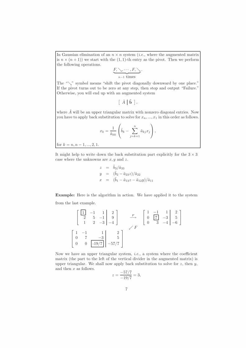
Example: Here is the algorithm in action. We have applied it to the system

from the last example.

1 −1 1 22 5 −1 91 2 −3 −4

F−→

1 −1 1 2

0 7 −3 50 3 −4 −6

ւ F

1 −1 1 20 7 −3 5

0 0 -19/7 −57/7

Now we have an upper triangular system, i.e., a system where the coefficientmatrix (the part to the left of the vertical divider in the augmented matrix) isupper triangular. We shall now apply back substitution to solve for z, then y,and then x as follows.

z =−57/7

−19/7= 3,

7

and

y =1

7(5 + 3z) =

5 + 3× 3

7= 2,

and finally,x = 2 + y − z = 2 + 2− 3 = 1.

�

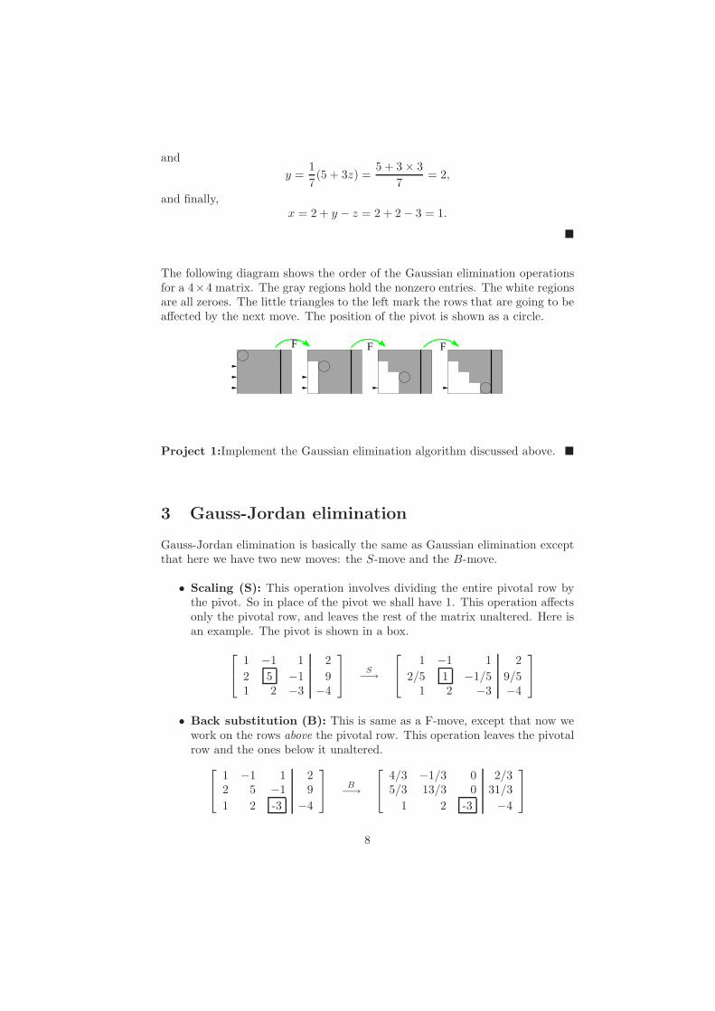
The following diagram shows the order of the Gaussian elimination operationsfor a 4×4 matrix. The gray regions hold the nonzero entries. The white regionsare all zeroes. The little triangles to the left mark the rows that are going to beaffected by the next move. The position of the pivot is shown as a circle.

F F F

Project 1:Implement the Gaussian elimination algorithm discussed above. �

3 Gauss-Jordan elimination

Gauss-Jordan elimination is basically the same as Gaussian elimination exceptthat here we have two new moves: the S-move and the B-move.

• Scaling (S): This operation involves dividing the entire pivotal row bythe pivot. So in place of the pivot we shall have 1. This operation affectsonly the pivotal row, and leaves the rest of the matrix unaltered. Here isan example. The pivot is shown in a box.

1 −1 1 2

2 5 −1 91 2 −3 −4

S−→

1 −1 1 2

2/5 1 −1/5 9/51 2 −3 −4

• Back substitution (B): This is same as a F-move, except that now wework on the rows above the pivotal row. This operation leaves the pivotalrow and the ones below it unaltered.

1 −1 1 22 5 −1 9

1 2 -3 −4

B−→

4/3 −1/3 0 2/35/3 13/3 0 31/3

1 2 -3 −4

8

Here we have subtracted 13 times the last row from the second row, and added

13 times the last row to the first row.

In Gauss-Jordan elimination of a n × n system we start with the pivot at the(1, 1)-th position. Then we perform the following operations.

S, F, B,ց, · · · , S, F, B,ց︸︷︷︸

n−1 times

, S, B.

As before the “ց” symbol means “shift the pivot diagonally downward by oneplace.”

Example: Let us perform Gauss-Jordan elimination for the same system. We

start with the original system in augmented matrix form.

1 −1 1 22 5 −1 91 2 −3 −4

(S,F )−→

1 −1 1 2

0 7 −3 50 3 −4 −6

↓ (S, F, B)

1 0 0 10 1 0 20 0 1 3

(S,B)←−

1 0 4/7 19/70 1 −3/7 5/7

0 0 -19/7 −57/7

�

4 Pivoting strategies

We have already mentioned the three basic steps: B,F, and S. All these stepsinvolve division by the pivot. So the pivot needs to be nonzero. However, it mayhappen that while performing the elimination the pivot turns out to be zero.Then we need to swap rows and/or columns to bring a nonzero number in theposition of the pivot. This is called pivoting. Pivoting is useful even when thepivot is nonzero, but is very small in absolute value. This is because, divisionby numbers new zero introduces large errors in the computer output. We shalldiscuss two pivoting strategies: partial pivoting, and complete pivoting.

4.1 Partial pivoting

Partial pivoting involves swapping rows. Suppose that at some step in theGaussian or Gauss-Jordan algorithm you have the following augmented matrix,

9

where the pivot is shown in a box.

1 2 3 62 −9 4 −3−5 1 2 −2

To perform partial pivoting look at the pivot as well as all the entries below thepivot in the pivotal column. These are shown bold. Locate among these theentry with the maximum absolute value. Here it is −5. Swap the pivotal rowwith with the row containing this entry. In this example we swap row 1 withrow 3 to get

-5 1 2 −22 −9 4 −31 2 3 6

Note that the position of the pivot (shown by the box) has remained unchanged,though the pivot itself has changed from 1 to −5.

In partial pivoting you look for a candidate pivot from among the current pivotand the entries below it:

Partial pivoting

Example: Here are some more examples of partial pivoting.

2 10 1 1

0 1 2 20 3 1 5

Pp

−→

2 10 1 1

0 3 1 50 1 2 2

10 3 4 310 1 3 52 13 8 9

Pp

−→

10 3 4 310 1 3 52 13 8 9

�

We have called the partial pivoting step as Pp. So now we have four differentkinds of steps: S, F, B and Pp.

10

In Gaussian elimination with partial pivoting we perform the following steps:

Pp, F,ց, · · · , Pp, F,ց︸︷︷︸

n−1 times

,

and then we perform back substitution as before. If the pivot turns out to bezero at any step (i.e., all the entries at and below the pivotal position are zerothen the system is singular, and the pivotal variable can be set to any value.For Gauss-Jordan elimination we do

Pp, S, F, B,ց, · · · , Pp, S, F, B,ց︸︷︷︸

n−1 times

, S, B.

4.2 Complete pivoting

In complete pivoting we swap rows and/or columns. Suppose the pivot is at the(i, i)-th entry. Then we look at all the (r, s)-th entries where r, s ≥ i.

Complete pivoting

Notice that we do not cross the vertical divider.

1 2 3 6

3 2 1 −54 1 −4 10

Locate the entry with the maximum absolute value among the bold entries. Ifthis is the (r, s)-th entry then swap i-th row of the augmented matrix with r-throw, and the i-column with the s-th column. Note that the order of row andcolumn swaps does not matter. In this example we swap row 2 with row 3, andcolumn 2 with column 3 to get

1 2 3 6

4 -4 1 103 1 2 −5

Recall that the columns of the matrix correspond to the variables of the equa-tions. So swapping the columns also involves reordering the variables. A simpleway to keep track of the order of the variables is to write the variables abovethe columns. If we call the variables as x, y, z in the last example then we shallwrite:

11

x y z1 2 3 6

3 2 1 −54 1 −4 10

Pc−→

x z y1 2 3 6

4 -4 1 103 1 2 −5

Here Pc is our symbol for complete pivoting.

In Gaussian elimination with complete pivoting we perform the following steps:

Pc, F,ց, · · · , Pc, F,ց︸︷︷︸

n−1 times

,

followed by back substitution as before. If we cannot avoid having a zero pivotat some step (i.e., all the entries at and to the south-east of the pivotal positionare zeros) then the system is singular, and the remaining variables (includingthe pivotal variable) can be set to any arbitrary value if the system is consistent.For Gauss-Jordan elimination we do

Pc, S, F, B,ց, · · · , Pc, S, F, B,ց︸︷︷︸

n−1 times

, S, B.

4.3 Keeping track of swaps

4.3.1 Method 1

There are two ways to keep track of the column swaps. Both uses an extra inte-ger array. In the first version we keep an integer array colPerm[0],...,colPerm[n-1],say. Initially colPerm[i] stores i for all i. This means all the columns are intheir right places to start with. Every time we swap two columns we also swapthe corresponding entries of the colPerm array.

Thus, at the end colPerm[i] stores the index of the variable at the i-th positionnow.

We need to find its inverse permutation, to know where a particular variable is.Remember that if π i a permutation, then its inverse permutation is π−1 where

∀i π−1(π(i)) = i.

So we can define a new array called, say, invColPerm[0,...,n-1] and fill it upas

for(i=0;i¡n;i++) invColPerm[colPerm[i]] = i;

Now the solution for the i-th variable can be found in a[invColPerm[i]][n].

12

4.3.2 Method 2

This is a conceptually simpler, though computationally more demanding solu-tion. Here we keep an integer array colIndex[0,...,n-1]. Instead of referringto the (i, j)-th entry of A as a[i][j]we shall use a[i][colIndex[j]]. Initially,colIndex[i] will store i for all i = 0, ..., n− 1. So a[i][colIndex[j]] will bethe same as a[i][j]. When we need to swap two columns we shall insteadonly swap the corresponding elements of colIndex. The following example willmake things clear.

Example: Let n = 3. After we swap columns 0 and 1, we have

colIndex[0] = 1, colIndex[1] = 0, colIndex[2] = 2.

So the (0, 1)-th entry of the new matrix is now a[0][colIndex[1]], which isa[0][0], as it should be.

If we perform the entire Gauss-Jordan algorithm like this, then there is no needto change anything at the end. The last c9olumn of the final augmented matrixwill automatically store the required solution in the correct order! �

Exercise 1:Show that the operations F, S and B all correspond to premultiplication

by special matrices. These matrices are called elementary matrices. Write down

the elementary matrices for performing these three basic moves for an n × n matrix

assuming that the pivotal position is (i, i). What similar statement can you make about

Pp and Pc? Compute the product of the elementary matrices for S, F and B moves.

�

Project 2:Implement Gauss-Jordan elimination with complete pivoting. �

Exercise 2:Suppose that we want to solve multiple systems with a common coefficientmatrix but different r.h.s. vectors and unknown vectors.

Ax1 = b1

Ax2 = b2

...

Axk = bk.

This is the same as solving the matrix equation:

AX = B,

13

where the bi’s are the columns of B, and the xi’s are the columns of X. Here we canapply Gauss/Gauss-Jordan elimination with the augmented matrix:

[A | B].

Write a program to implement Gauss-Jordan elimination (with complete pivoting) in

this set up. �

5 Some theory behind Gauss-Jordan elimina-tion

Notice that we are using four basic actions: dividing a row by a number, sub-tracting multiple of one row from another, swapping two rows, and swappingtwo columns. Of these the first three are row operations and can be done byleft multiplication with elementary matrices. The last operation is a columnoperation, and hence done by right multiplication. If we accumulate all the leftand right marices then at the end of Gauss-Jordan elimination we are left with

LAR = I.

So A = L−1R−1, orA−1 = RL.

Convince yourself that left multiplying by R is same as applying the columnswaps to the rows in the reverse order.

From now on we shall assume that R = I for ease of exposition. The resultsshould be easily modifiable for general R.

Here is another interesting point. After p steps the matrix is of the form[

Ip P b1

O Q b2

]

.

When does total pivoting fail? When Q = O. Thus the system is inconsistentif b2 6= 0. If b2 = 0 then the general solution is y arbitrary and x = b1 − Py.

Another interesting point is

Q = A22 −A21A−111 A12.

This is because if all the accumulated left multiplier matrix is L then it is ofthe form

L =

[Up×p VW I

]

.

Do you see why the lower right hand block is I? Now we have

LA =

[Up×p VW I

] [A11 A12

A21 A22

]

=

[Ip PO Q

]

.

14

SoQ = W A12 + A22.

To find W we note that W A11 + A21 = O, or

W = −A21A−111 .

So combining everything we have

Q = A22 −A21A−111 A12.

an easy proof by just performing the block matrix multiplication. This resultis useful because we often have to compute the rhs in statistics. It is called theconditional covariance matrix.

6 Inversion using Gauss-Jordan elimination

Gauss-Jordan elimination (with pivoting) may be used to find inverse of a givennonsingular square matrix, since finding inverse is the same as solving the system

AX = I.

Example: Suppose that we want to find the inverse of the matrix

1 −1 12 5 −11 2 −3

.

Then we append an identity matrix of the same size to the right of this matrixto get the augmented matrix

1 −1 1 1 0 02 5 −1 0 1 01 2 −3 0 0 1

.

Now go on applying Gauss-Jordan elimination until the left hand matrix isreduced to identity. The right hand at the final step will give the requiredinverse. Each step combines the S,F and B-moves.

1 −1 1 1 0 02 5 −1 0 1 01 2 −3 0 0 1

(S,F )−→

1 −1 1 1 0 00 7 −3 −2 1 00 3 −4 −1 0 1

After a set of S, F and B steps we arrive at

1 0 4/7 5/7 1/7 00 1 -3/7 -2/7 1/7 00 0 -19/7 -1/7 -3/7 1

,

15

which after the final S, B steps yields

1 0 0 91/133 7/133 4/190 1 0 -35/133 28/133 -3/190 0 1 1/19 3/19 -7/19

Thus, the required inverse is

91/133 7/133 4/19-35/133 28/133 -3/191/19 3/19 -7/19

.

�

6.1 Efficient implementation

First consider the case where we do not need to perform any row/column swap.Then we start out like this:

∗ ∗ ∗ 1 0 0∗ ∗ ∗ 0 1 0∗ ∗ ∗ 0 0 1

.

Here a ∗ denotes an entry that depends on the matrix being inverted. After onesweep we have

1 ∗ ∗ ∗ 0 00 ∗ ∗ ∗ 1 00 ∗ ∗ ∗ 0 1

.

Notice that the first column is now forced to be (1, 0, 0)′. After another step wehave

1 0 ∗ ∗ ∗ 00 1 ∗ ∗ ∗ 00 0 ∗ ∗ ∗ 1

.

After the third step we have

1 0 0 ∗ ∗ ∗0 1 0 ∗ ∗ ∗0 0 1 ∗ ∗ ∗

.

The ∗’s in the right hand half now constitute the inverse matrix. Notice thatat each step there are exactly as many ∗’s as there are entries in the originalmatrix. Clearly, all that we really need to store are the ∗’s, because the othrentries are anyway constants irrespective of the matrix being being inverted.

It should not be difficult to check that the following algorithm computes the ∗’s:

16

For p = 0 to n− 1 you compute

aij = aij −aipapj

app

i, j 6= p

aip = −aip/app i 6= p

apj = apj/app j 6= p

app = 1/app.

Then in the above algorithm the i-th column of A is needed only to compute thei-column of A−1. So we can overwrite the i-th column of A with the i-th columnof A−1 to save space. This is an example of an in place algorithm, i.e., wherethe output gradually overwrites the input. If we need to perform row/columnswaps, then the situation is very similar. To see this consider the same exampleonce again. We start out as

∗ ∗ ∗ 1 0 0∗ ∗ ∗ 0 1 0∗ ∗ ∗ 0 0 1

.

After one sweep we have

1 ∗ ∗ ∗ 0 00 ∗ ∗ ∗ 1 00 ∗ ∗ ∗ 0 1

.

Now suppose we swap the second and third rows:

1 ∗ ∗ ∗ 0 00 ∗ ∗ ∗ 0 10 ∗ ∗ ∗ 1 0

.

The next sweep will produce

1 0 ∗ ∗ 0 ∗0 1 ∗ ∗ 0 ∗0 0 ∗ ∗ 1 ∗

.

Notice that we still have exactly the same number of ∗’s, but now they are nomore side by side.

The third sweep will yield

1 0 0 ∗ ∗ ∗0 1 0 ∗ ∗ ∗0 0 1 ∗ ∗ ∗

.

Here the right hand half stores the inverse of the row-swapped version of theoriginal matrix, i.e., (LA)−1, where L is the row-swap matrix. Now (LA)−1 =A−1L−1. Hence

A−1 = (LA)−1L.

17

When L is multiplied from the right, it swaps the columns in the reverse order.

Thus we need to keep track of the swaps and apply them in the reverse orderto the inverse. Remember that a row swap becomes a column swap and viceversa.

Project 3:Implement the in-place version of the Gauss-Jordan inversion algo-rithm using complete pivoting. �

7 Determinant using Gaussian elimination

One may use the Gaussian elimination or Gauss-Jordan elimination algorithmto compute the determinant.

Start by applying the n− 1 moves of type (Pc, F ), as in Gaussian elimination.Then multiply the diagonal entries of the resulting matrix. If you have donek row/col swaps, then multiply with (−1)k. A row swap is counted separatelyfrom a column swap.

Project 4:Implement the above algorithm to compute the determinant of agiven square matrix. �

8 LU decompositions

We say that a nonsingular matrix has LU decomposition if it can be written as

A = LU,

where L is a lower triangular and U is an upper triangular matrix.

Exercise 3:Show that such a factorization need not be unique even if one exists. �

If L has 1’s on its diagonals then it is called Doolittle decomposition and if Uhas 1’s on its diagonals, it is called Crout’s factorization. If L = U ′ then we callit Cholesky decomposition (read Cholesky as Kolesky.)

We shall work with Crout’s decomposition as a representative LU decomposi-tion. The others are similar.

18

8.1 Application

LU decomposition is mainly used as a substitute for matrix inversion. If A = LUthen you can solve Ax = b as follows.

First write the system as two triangular systems

Ly = b, where y = Ux.

Being triangular, the systems can be solved by forward or backward substitution.Apply forward substitution to solve for y from the first eqation, and then applybackward substitution to solve for x from the second equation.

Notice that, unlike Gausian/Gauss-Jordan elimination, we do not need to knowb while computing the LU decomposition. This is useful when we want to solvemany systems of the form Ax = b where A is always the same, but b willchange later depending on the situation. Then the LU decomposition needs tobe computed once and for all. Only the two substitutions are to be done afreshfor each new b.

8.2 Algorithm

From definition of matrix multiplication we have

aij =

n∑

k=1

likukj .

Now, lik = 0 if k > i, and ukj = 0 if k < j. So the above sum is effectively

aij =

min{i,j}∑

k=1

likukj .

You can compute li1 ’s for i ≥ 1 by considering

ai1 = li1u11 = li1,

since diagonal entries of U are 1. Once l11 has been computed you can computeu1i’s for i ≥ 2 by considering

u1i = a1i/l11.

Next you will compute li2’s and after that u2i’s, and so on. The order in whichyou compute the lij ’s and uij ’s is shown in the diagram below.

13

57

9 10

1311 12

24

68

= one

= zeroL = U =

LU decomposition computation order

19

The general formulas to compute lij and uij are

lij = aij −∑j−1

k=1 likukj (i ≥ j)

uij = 1lii

(

aij −∑i−1

k=1 likukj

)

(i < j).

Exercise 4:What should we do if for some i we have lii = 0? Does this necessarily

mean that LU decomposition does not exist in this case? �


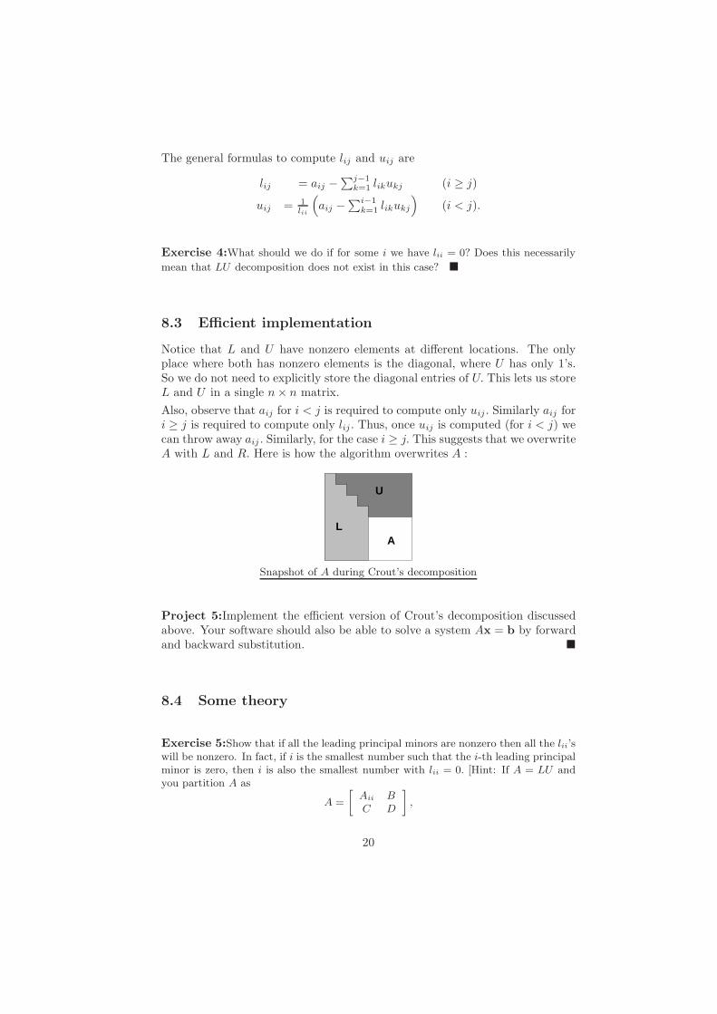
Notice that L and U have nonzero elements at different locations. The onlyplace where both has nonzero elements is the diagonal, where U has only 1’s.So we do not need to explicitly store the diagonal entries of U. This lets us storeL and U in a single n× n matrix.

Also, observe that aij for i < j is required to compute only uij . Similarly aij fori ≥ j is required to compute only lij . Thus, once uij is computed (for i < j) wecan throw away aij . Similarly, for the case i ≥ j. This suggests that we overwriteA with L and R. Here is how the algorithm overwrites A :

L

U

A

Snapshot of A during Crout’s decomposition

Project 5:Implement the efficient version of Crout’s decomposition discussedabove. Your software should also be able to solve a system Ax = b by forwardand backward substitution. �

8.4 Some theory

Exercise 5:Show that if all the leading principal minors are nonzero then all the lii’swill be nonzero. In fact, if i is the smallest number such that the i-th leading principalminor is zero, then i is also the smallest number with lii = 0. [Hint: If A = LU andyou partition A as

A =

»

Aii BC D

–

,

20

where Aii is i × i, then what is the LU decomposition of Aii? Now apply the formulafor determinant of partitioned matrix to show that

lii = |Aii|/|Ai−1,i−1|.

�

Exercise 6:Use the above exercises to characterize all square matrices having LU

decomposition. �

9 QR decomposition

Theorem

For any n by p matrix A with n ≥ p we have an n by n orthogonal matrix Qand an n by p upper triangular matrix R such that

A = QR.

This decomposition is the matrix version of Gram-Schmidt Orthogonalization(GSO). To see this we first consider the case where A is full column rank (i.e.,the columns are independent.) Call the columns

a1, ..., ap.

Apply GSO to get an orthonormal set of vectors

q1, ..., qp

given by

qi = unit(ai −

i−1∑

j=1

q′jai)

computed in the order i = 1, ..., p. Here unit(v) denotes the unit vector

unit(v) = v/‖v‖,

for any nonzero v. If v = 0, then unit(v) is not defined.

Notice that ai is a linear combination of q1, ..., qi only and not of qi+1, ..., qp. Sowe can write

qi = r1ia1 + r2ia2 + · · ·+ riiai.

Define the matrix R using the rij ’s.

21

If A is not full column rank then some (ai −∑i−1

j=1 q′jai) will be zero, hence wecannot apply unit to it. But then we can take qi equal to any unit norm vectororthogonal to q1, ..., qi−1 and set rii = 0.

However, GSO is not the best way to compute QR decomposition of a ma-trix. This is because in the unit steps you have to divide by the norms whichmay be too small. The standard way to implement it is using Householder’stransformation.

9.1 Householder’s transformation

If A is any orthogonal matrix then

‖Ax‖ = ‖x‖.

In other words an orthogonal matrix does not change shape or size. It can onlyrotate and reflect objects. We want to ask if the reverse is true: if x and y aretwo vectors of same length then does there exist an orthogonal A that takesx to y and vice versa? That is, we are looking for an orthogonal A (possiblydepending on x, y) such that

Ax = y and Ay = x?

The answer is “Yes.” In fact, there may be many. Householder’s transform isone such:

A = I − 2uu′, where u = unit(x− y).

Exercise 7:Show that this A is orthogonal and it sends x to y and vice versa. �

Exercise 8:Show that in 2 dimensions Householder’s transform is the only such

transform. Show that this uniqueness does not hold for higher dimensions. �

Exercise 9:In general you need n2 scalar multiplications to multiply an n×n matrix

with an n × 1 vector. However, show that if the matrix is a Householder matrix then

only 2n scalar multiplications are needed. �

9.2 Using Householder for QR

The idea is to shave the columns of X one by one by multiplying with House-holder matrices. For any non zero vector u define Hu as the Householder matrix

22

that reduces u to

v =

‖u‖2

0...0

.

Exercise 10:Let us partition a vector u as

un×1 =

»

u1

u2

–

,

where both u1,u2 are vectors (u2 being k × 1). Consider the n × n matrix

H =

»

I 00 Hu2

–

.

Show that H is orthogonal and compute Hu. We shall say that H shaves the last k−1

elements of u. �

Let the first column of X be a. Let H1 shave its lower n− 1 entries. Considerthe second column b of H1A. Let H2 shave off its lower n− 2 entries. Next let cdenote the third column of H2H1X, and so on. Proceeding in this way, we getH1, H2, ..., Hp all of which are orthogonal Householder matrices. Define

Q = (H1H2 · · ·Hp)′

and R = Q′X to get a QR decomposition.

Exercise 11:Carry this out for the following 5 × 4 case.2

6

6

6

6

4

1 2 3 41 3 2 41 −2 5 07 2 1 3−2 8 5 4

3

7

7

7

7

5

�


Notice that though the Householder matrix

I − 2uu′

is an n× n matrix, it is actually determined by only n numbers. Thus, we caneffectively store the matrix in linear space. In particular, the matrix H1 needsonly n spaces, H2 needs only n− 1 spaces and so on.

23

So we shall try to store these in the “shaved” parts of X. Let H1 = 1 − 2u1u′1

and H1X be partitioned as [α v′

0 X1

]

.

Then we shall try to store u1 in place of the 0’s. But u1 is an n × 1 vector,while we have only n−1 zeroes. So the standard practice is to store α (which isthe squared norm of the first column) in a separate array, and store u1 in placeof the first column of A.

The final output will be a n×p matrix and a p-dimensional vector (which is likean extra row in A). The matrix is packed with the u’s and the strictly uppertriangular part of R :

6u

5u4u

3u2u

1u

of Rdiagonal entries

part of Rstrict upper triangular

Output of efficient QR decomposition

The “extra row” stores the diagonal entries of R. It is possible to “unpack” Qfrom the u’s. However, if we need Q only to multiply some x to get Qx, theneven this unpacking is not necessary.

Exercise 12:Write a program that performs the above multiplication without ex-

plicitly computing Q. �

Project 6:Write a program to implement the above efficient version of QRdecomposition of a full column rank matrix A. Your program should be able todetect if A is not full column rank, in which case it should stop with an errormessage. �

This is not entirely easy to do. So let’s proceed step by step. First we chalk outthe basic flowchart.

24

for i = 0, ..., p− 1

Read n, p,A

"Shave" the lower olumn of A.

part of the i-thThe main algo

The easiest part to expand here is the input part. The only subtlety is toremember to allocate an extra row in A.

partthe top n× p

Read A intofor An+1×p

Allo ate memoryRead n, p

The input part

Now comes the tricky step: the “shaving”. There are two parts here. First, wehave to compute the u vector, and save it in the A matrix. Second, we have tomultiply the later columns by Hu.

25

Pro ess olumn i.

Update olumn j

for j = i + 1, ..., p− 1

How to “shave”

The flowchart below is quite technical in nature. It tells you how to computethe u vector, and save it in the A matrix. It also saves the diagonal element ofR in the “extra row” of A.

normsq1 =∑n−1

j=i+1a2

ji

norm =√

normsq1 + a2ii

normDiff =√

normsq1 + a2ii

aii = aii − norm

Divide aii, ..., an−1,i by normDiff

Store norm in ani

Processing the ”shaved” column (i)

Updating the subsequent columns is basically multiplying by a Householdermatrix.

26

akj = akj −mult ∗ aki

for k = i, ..., n− 1

mult = 2∑n−1

k=i akiakj

Updating column j

9.4 Application to least squares

An important use is in solving least squares problems. Here we are given a(possibly inconsistent) system

Ax = b,

where A is full column rank (need not be square.) Then we have the followingtheorem.

Theorem

The above system has unique least square solution x given by

x = A(A′A)−1A′b.

Note that the full column rankness of A guarantees the existence of the inverse.

However, computing the inverse directly and then performing matrix multipli-cation is not an efficient algorithm. A better way (which is used in standardsoftware packages) is to first form a QR decomposition of A as A = QR. Thegiven system now looks like

QRx = b.

The lower part of R is made of zeros:

Q

[R1

O

]

x = b,

or [R1

O

]

x = Q′b,

Partition Q′b appropriately to get

[R1

O

]

x =

[c1

c2

]

,

where c1 is p× 1. This system is made of two systems:

R1x = c1

27

andOx = c2.

The first system is always consistent and can be solved by back-substitution.The second system is trivial and inconsistent unless c2 = 0.

Exercise 13:Show that x = R−1

1c1 is the least square solution of the original system.

Notice that you use back-substituting to find this x and not direct inversion of R1. �

Exercise 14:Find a use of c2 to compute the residual sum of squares:

‖b − Ax‖2.

�

28

-~arnabc-matalgop1.pdf

Documents