Αλγοριθμική Θεωρία Γραφημάτων

Αλγοριθμική Θεωρία Γραφημάτων

Διάλεξη 3

Τριγωνικά ΓραφήματαΜεταβατικά Γραφήματα

. Σταύρος Δ Νικολόπουλος1

Triangulated Graphs

Perfect Elimination Ordering

2

Algorithmic Graph Theory

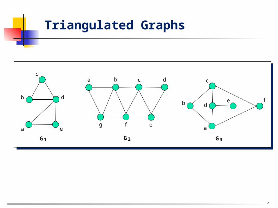
G triangulated G has the triangulated graph property

Every simple cycle of length l > 3 possesses a chord.

Triangulated graphs, or

Chordal graphs, or

Perfect Elimination Graphs

Triangulated Graphs

3

c

b

a

e fd

c

b

a e

d

G G1 3G2

a

g e

b c d

f

4

Triangulated Graphs

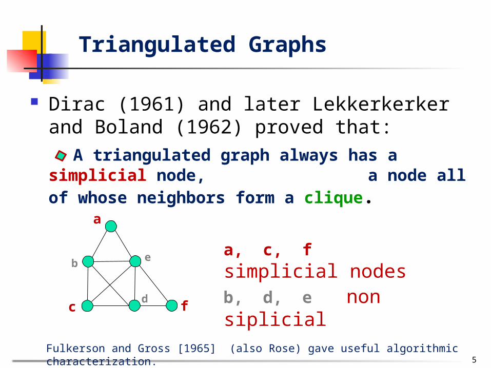
Dirac (1961) and later Lekkerkerker and Boland (1962) proved that:

A triangulated graph always has a simplicial node, a node all of whose neighbors form a clique.

a

b

cd

f

e a, c, f simplicial nodesb, d, e non siplicial

5

Triangulated Graphs

Fulkerson and Gross [1965] (also Rose) gave useful algorithmic characterization.

It follows easily from the triangulated property that:

deleting nodes of a triangulated graph yields another triangulated graph.

a

b

cd

f

e

a

b

cd

f

a

b

df

e

6

Triangulated Graphs

Recognition AlgorithmThis observation leads to the following easy and simple

recognition algorithm:

Find a simplicial node of G;

Delete it from G, resulting G’;

Recourse on the resulting graph G’, until no node remain.

7

Triangulated Graphs

If G contains a Ck, k 4, no node in that cycle will ever become simplicial.

8

Triangulated Graphs

Triangulated Non-triangulated

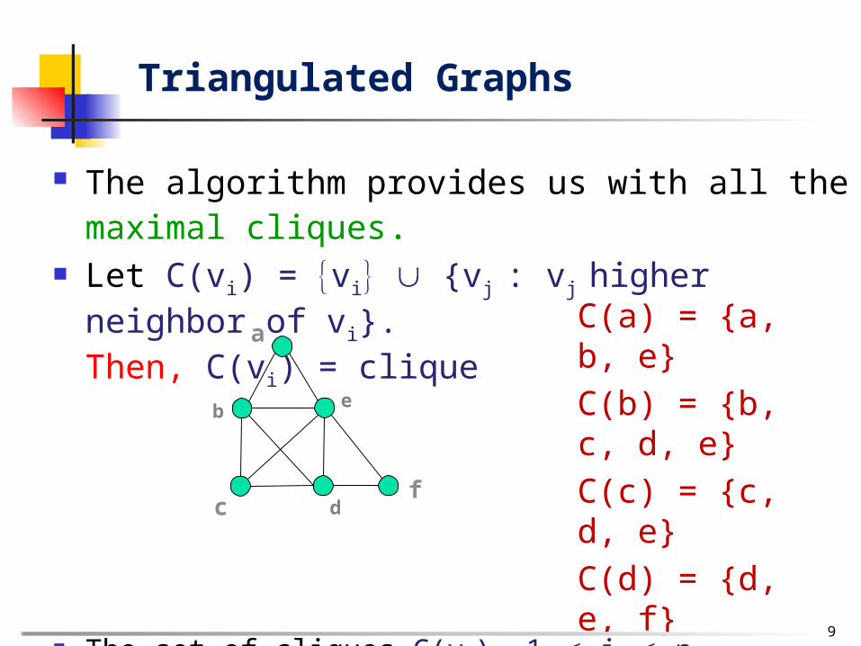
The algorithm provides us with all the maximal cliques. Let C(vi) = vi {vj : vj higher neighbor of vi}.

Then, C(vi) = clique

The set of cliques C(vi), 1 i n ,

includes all the maximal cliques.

a

b

c df

e

C(a) = {a, b, e}

C(b) = {b, c, d, e}

C(c) = {c, d, e}

C(d) = {d, e, f}

C(e) = {e, f}

C(f) = {f}

9

Triangulated Graphs

Note that some cliques C(vi) are not maximal.

C(a) = {a, b, e}

C(b) = {b, c, d, e}

C(c) = {c, d, e}

C(d) = {d, e, f}

C(e) = {e, f}

C(f) = {f}

10

Triangulated Graphs

a

b

c df

e

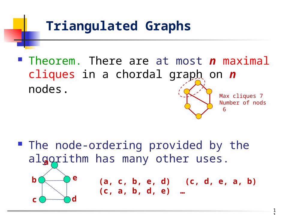
Theorem. There are at most n maximal cliques in a chordal graph on n nodes.

The node-ordering provided by the algorithm has many other uses.

Max cliques 7Number of nods 6

a

b

c d

e (a, c, b, e, d) (c, d, e, a, b) (c, a, b, d, e) …

11

Triangulated Graphs

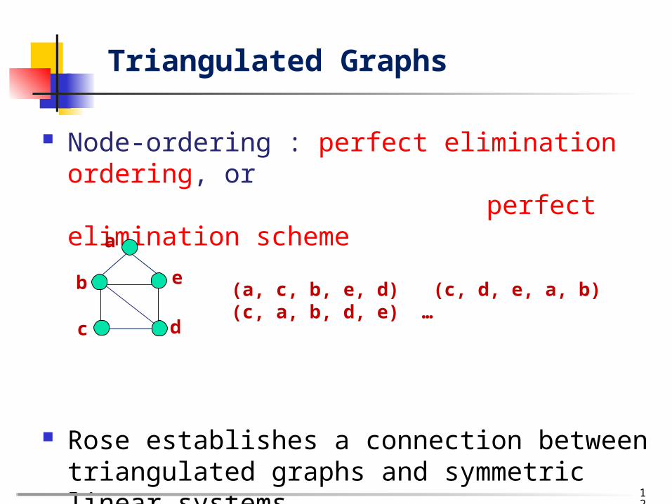
Node-ordering : perfect elimination ordering, or perfect elimination scheme

Rose establishes a connection between triangulated graphs and symmetric linear systems

(a, c, b, e, d) (c, d, e, a, b) (c, a, b, d, e) …

a

b

c d

e

12

Triangulated Graphs

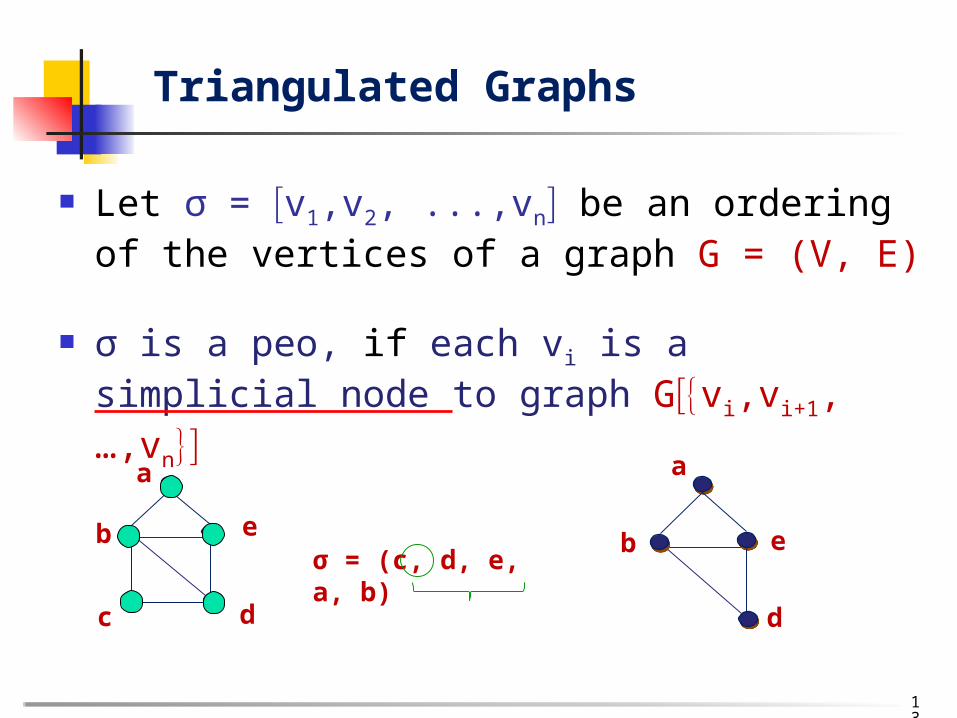
Let σ = v1,v2, ...,vn be an ordering of the vertices of a graph G = (V, E)

σ is a peo, if each vi is a simplicial node to graph Gvi,vi+1, …,vn

a

b

c d

eσ = (c, d, e, a, b)

a

b

d

e

13

Triangulated Graphs

σ is a peo if each vi is a simplicial node to graph Gvi,vi+1, …,vn. That is,

Xi= vj adj (vi) i < j is complete.

σ =1, 7, 2, 6, 3, 5, 4 no simplicial vertex G1 has 96 different peo.

14

c

b

a

e fd

G2

G1

a

g e

b c d

f

Triangulated Graphs

Algorithm LexBFS

Algorithm MCS

15


Algorithm LexBFS

1. for all vV do label(v) : () ;2. for i : V down to 1 do

2.1 choose vV with lexmax label (v);2.1 σ (i) v;2.3 for all u V ∩N(v) do

label (u) label (u) || i2.4 V V \ v;

end

16

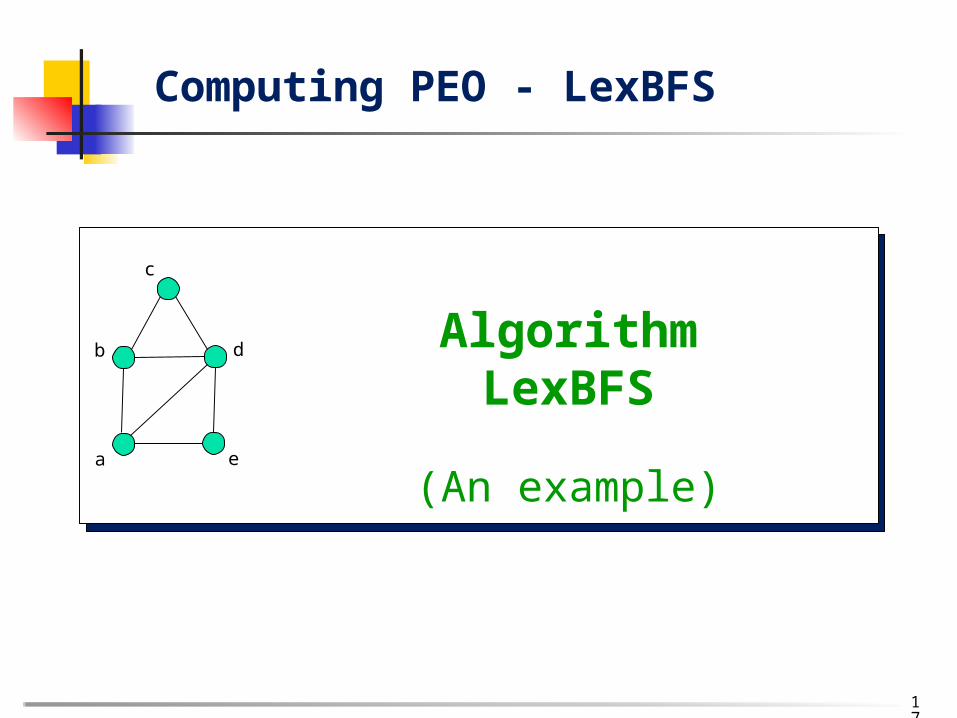
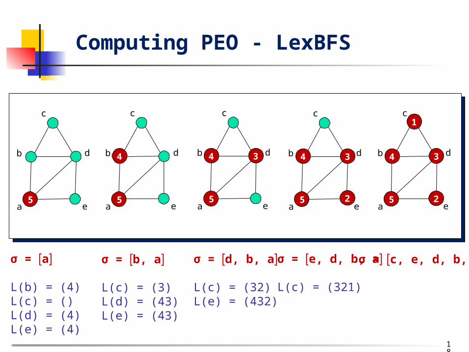
Computing PEO - LexBFS

17


c

b

a e

d Algorithm LexBFS

(An example)

c

b

a e

d

c

b

a e

d

c

b

a e

d

c

b

a e

d

c

b

a e

d

1

5 5 5 5 5

4 4 4 43 3 3

2 2

= σ a

L(b) = (4)L(c) = () L(d) = (4)L(e) = (4)

= σ b, a

L(c) = (3) L(d) = (43)L(e) = (43)

= σ d, b, a

L(c) = (32) L(e) = (432)

= σ e, d, b, a

L(c) = (321)

= σ c, e, d, b, a

18


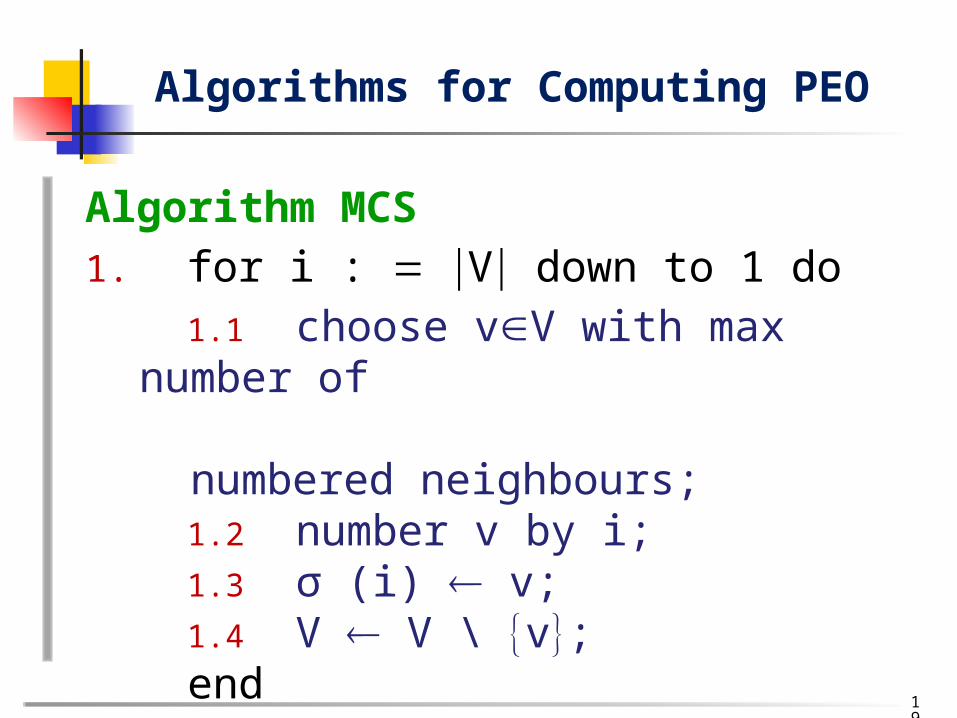
Algorithm MCS

1. for i : V down to 1 do

1.1 choose vV with max number of numbered neighbours;

1.2 number v by i;1.3 σ (i) v;1.4 V V \ v;

end

Algorithms for Computing PEO

19

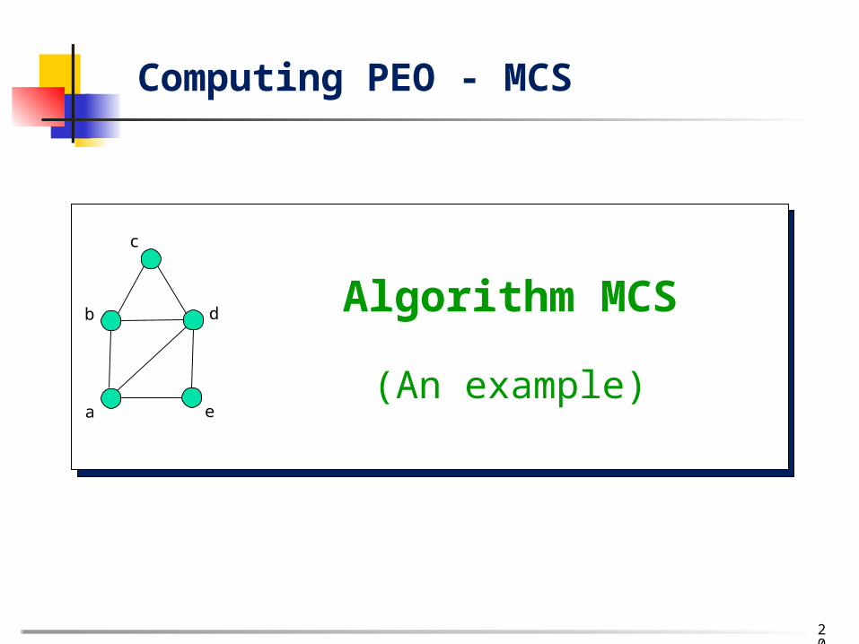
c

b

a e

d

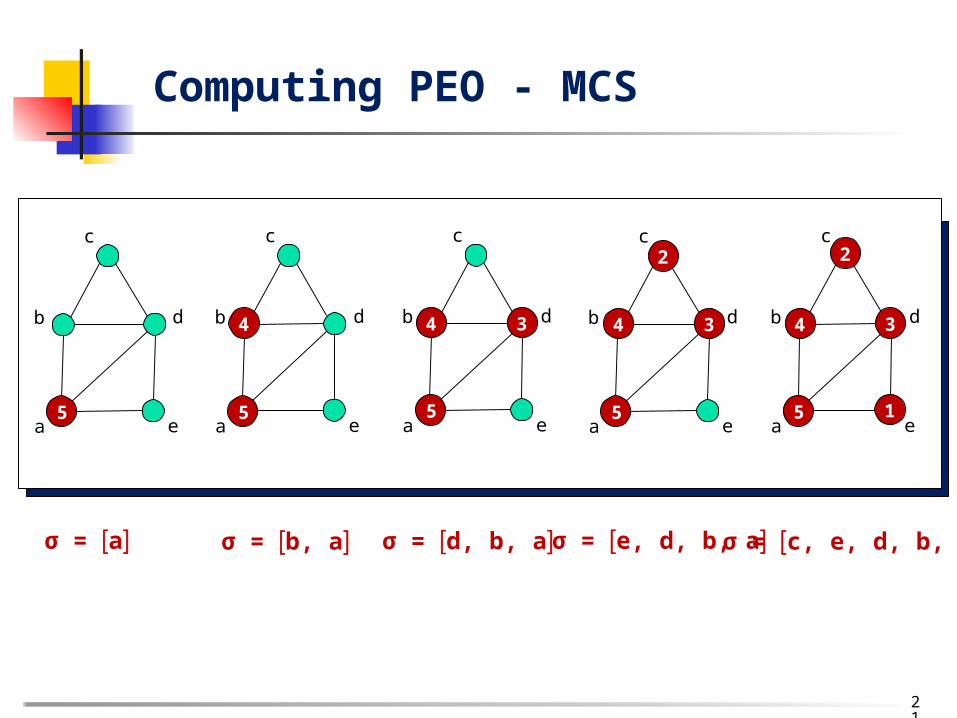
Computing PEO - MCS

20

Algorithm MCS

(An example)

c

b

a e

d

c

b

a e

d

c

b

a e

d

c

b

a e

d

c

b

a e

d

2

5 5 5 5 5

4 4 4 43 3 3

1

2

= σ a = σ b, a = σ d, b, a = σ e, d, b, a = σ c, e, d, b, a

21

Computing PEO - MCS

Algorithms LexBFS & MCS

22

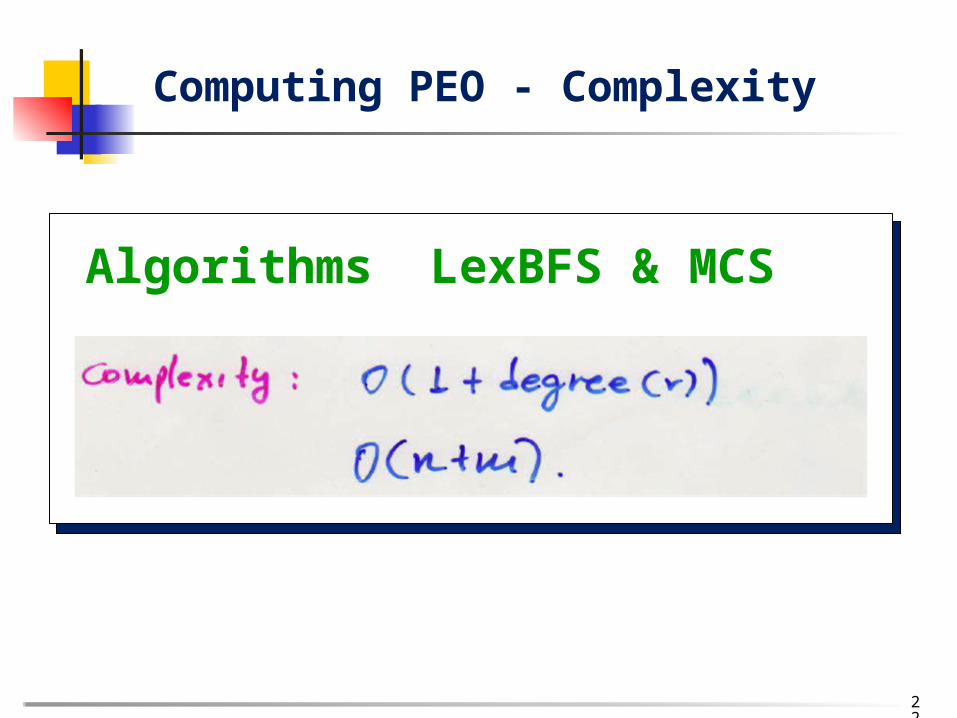
Computing PEO - Complexity

Algorithm PERFECT

Correctness & Complexity

23


Algorithm PERFECT

1. for all vertices u do A(u) Ø;2. for i 1 to n-1 do 3. v σ(i);4. Xv x adj(v) | σ-1(v) < σ-1(x) ;5. if Xv = Ø then goto 8

6. u σ (min σ-1(x) xXv );7. A(u) A(u) Xv-u8. if A(v) - adj (v) Ø then return (“false”)9. end 10. return (“true”)

Naive Algorithm O(n3)

This Algorithm O(n+m)

A(v) adj(v) true

24

Testing a PEO – Algorithm PERFECT

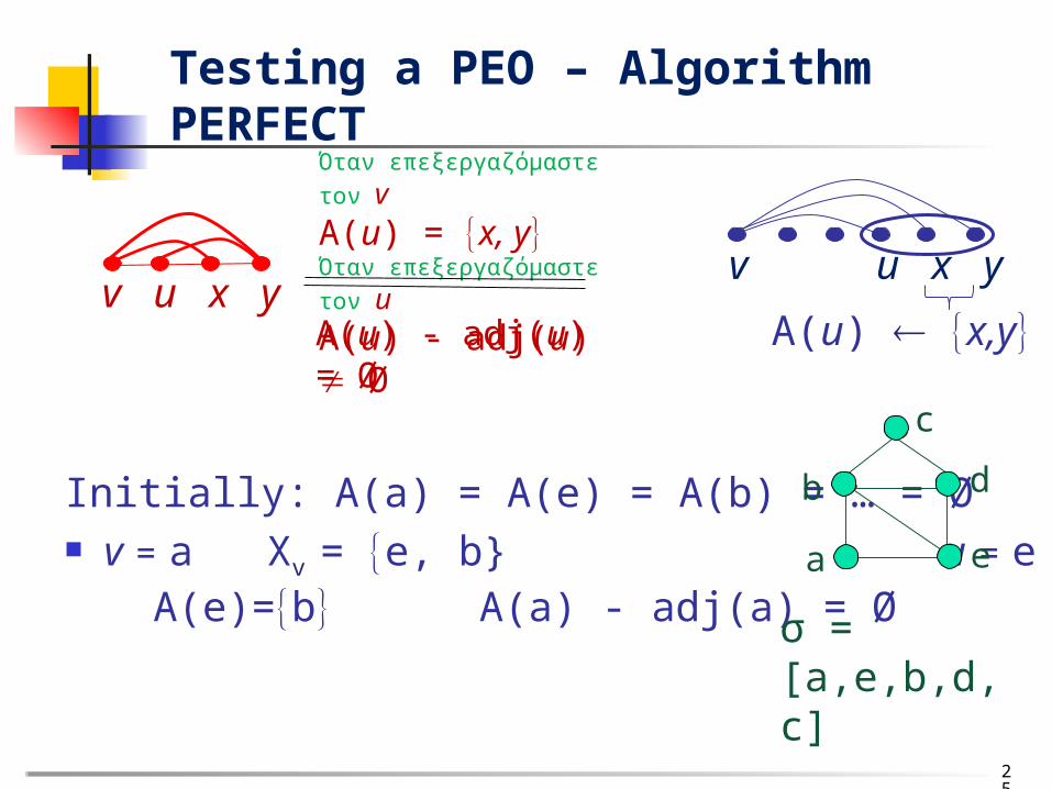
Initially: A(a) = A(e) = A(b) = … = Ø v = a Xv = e, b} u = e

A(e)=b A(a) - adj(a) = Ø

v = e Xv = b, d u = b A(b) = d A(e) - adj(e) = Ø

… 25

b

c

d

ea

σ = [a,e,b,d,c]

v u x yv u x y

A(u) x,y


A(u) - adj(u) = Ø

Όταν επεξεργαζόμαστε τον v

A(u) = x, yΌταν επεξεργαζόμαστε τον u

A(u) - adj(u) Ø

Example (a):

σ = [1, 2, 3, 4, 5, 6, 7, 8]

v = 1: Xv={3,4,8} u = 3 A(3)={4,8} A(1) - adj(1)v = 2: Xv={4,7} u = 4 A(4)={7} A(2) - adj(2)v = 3: Xv={4,5,8} u = 4 A(4)={7,5,8} A(3) - adj(3)v = 4: Xv={5,7,8} u = 5 A(5)={7,8} A(4) - adj(4)v = 5: Xv={6,7,8} u = 6 A(6)={7,8} A(5) - adj(5)v = 6: Xv={7,8} u = 7 A(7)={8} A(6) - adj(6)

26


Theorem: The algorithm PERFECT returns TRUE

iff σ is a peoProof :() Suppose that the algorithm returns FALSE during

the σ-1(u)-th iteration. This may happen only if in line 8:

A(u) - adj(u)

Thus, w A(u) such that w adj(u)

Correctness of Algorithm PERFECT

27

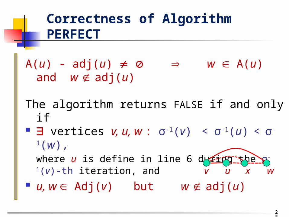
A(u) - adj(u) w A(u) and w adj(u)

The algorithm returns FALSE if and only if vertices v, u, w : σ-1(v) < σ-1(u) < σ-1(w),

where u is define in line 6 during the σ-1(v)-th iteration, and

u, w Adj(v) but w adj(u)

Clearly, since (u,w) E σ is not peo.

v u x w

28


() Suppose σ is not a peo and the Algo PERFECT returns TRUE.

Let v be a vertex with max index in σ, such that

Xv=w w adj(v) and σ-1(v) < σ-1(w)

is not complete

σ = [………v,….….....…..]

max

29


i.e., v is the first vertex from right to left in σ s.t Xv does not induce a clique

Let u be a vertex of set Xv

defined during the σ-1(v)-th iteration (in line 6),

after which (in line 7)

Xv-{u} is added to A(u)

1st neighbor

σ = [………v,…..,u,……..]

30


Since the Algorithm PERFECT

returns TRUE A(u) - adj(u) = (in line 8)

Xv-{u} adj (u)

31


maxA(u)

σ = (……, v, …, u, ……..)

v

u X - {u}v

X - {u}

v

Thus, (i) every x Xv -{u} is adjacent to u.

x

32


maxA(u)

σ = (……, v, …, u, ……..)

v

u X - {u}v

X - {u}

v

(i) every x Xv -{u} is adjacent to u.

xand

(ii) every x, y Xv -{u} is adjacent.

y

Statement (ii) follows since v is the vertex with max index in σ such that Xv is not completeThus, Xv is complete, a contradiction!

Chromatic Number

Clique Number - Max Clique

Stability Number α(G)

33


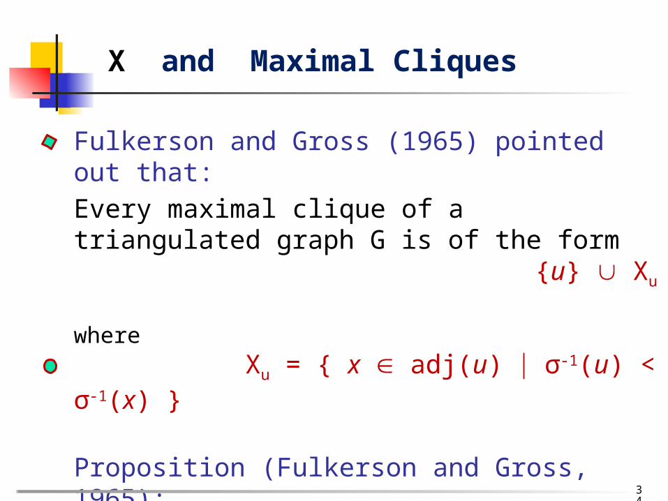
Fulkerson and Gross (1965) pointed out that:

Every maximal clique of a triangulated graph G is of the form {u} Xu where Xu = { x adj(u) σ-1(u) < σ-1(x) }

Proposition (Fulkerson and Gross, 1965):

A triangulated graph on n nodes has at most n maximal cliques, with equality iff the graph has no edges.

X and Maximal Cliques

34

Algorithm Maximalcliques Some of {u}Xu will not be maximal clique;

{u}Xu is not maximal clique if and only if

for some i, in line 7 of Algorithm PERFECT,

Xu = Xv-u is concatenated to A(u);

35

1, 2, …, i, …

uvXu


7. A(u) A(u) Xv-u

{u}Xu

Example (a):

{1}X1 ={1,6,7,8}

{2}X2 ={2,5,6}

{3}X3 ={3,5} {6}X6 ={6,7,8}

{4}X4 ={4,8} {7}X7 ={7,8}

{5}X5 ={5,6,7} {8}X8={8}

maximal non maximal

36

σ = [1, 2, 3, 4, 5, 6, 7, 8]


37


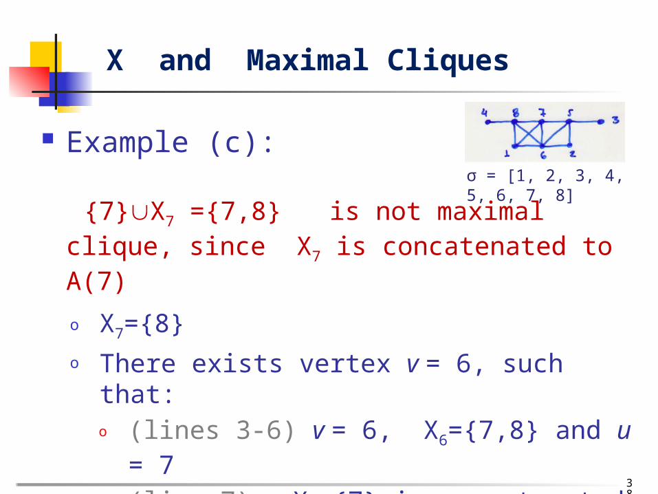
σ = [1, 2, 3, 4, 5, 6, 7, 8]

Example (b):

{6} X6={6,7,8} is not maximal clique, since X6 is concatenated to A(6)

o X6={7,8}o There exists vertex v = 1, such that:

o (lines 3-6) v = 1, X1={6,7,8} and u = 6

o (line 7) X1-{6} is concatenated to A(u)

o X1-{6} = {7,8} = X6 is concatenated to A(6)

38


σ = [1, 2, 3, 4, 5, 6, 7, 8]

Example (c):

{7}X7 ={7,8} is not maximal clique, since X7 is concatenated to A(7)

o X7={8}o There exists vertex v = 6, such that:

o (lines 3-6) v = 6, X6={7,8} and u = 7

o (line 7) X6-{7} is concatenated to A(u)

o X6-{7} = {8} = X7 is concatenated to A(7)

clique(σ)

X 1; S(v) 0 vV;1. for i 1 to n do 2. v σ(i)3. Xv {xadj(v) σ-1(v) < σ-1(x) }4. if adj(v) = Ø then print {v}; 5. u σ (min σ-1(x) xXv );6. if Xv = Ø then goto 9

7. S(u) max{S(u), Xv-1}8. if S(v) < Xv then do : print {v}Xv

9. end X = max {X, 1+ Xv }return X

Algorithm X and Maximal Clique

39

S(v) indicates the size of the largest set that would have

been concatenated to A(v) in Algorithm PERFECT.

Gavril (1972) gives a coloring algorithm, based on a greedy approach.

We use positive integers as colors.

Method: Start at the last node vn of the peo; Work backwards, assign to each vi in turn the

minimum color not assigned to its higher neighbors.

Coloring Chordal Graphs

40

Example:

σ = [a, c, b, d, e, f]

3 1 2 3 2 1

ω(G) = χ(G)

Coloring Chordal Graphs

41

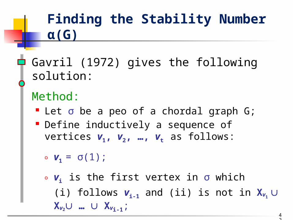
Gavril (1972) gives the following solution:

Method: Let σ be a peo of a chordal graph G; Define inductively a sequence of vertices v1, v2, …, vt as

follows:

o v1 = σ(1);

o vi is the first vertex in σ which

(i) follows vi-1 and (ii) is not in Xv1 Xv2 … Xvi-1;

Recall that, all vertices following vt are in Xv1 Xv2 … Xvt

Finding the Stability Number α(G)

42

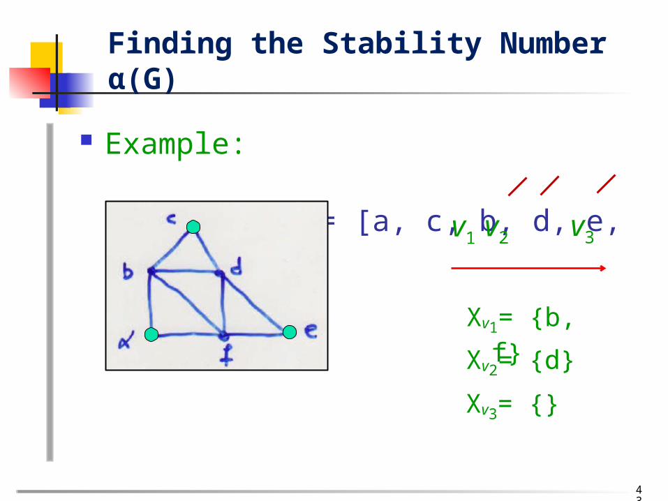
Example:

σ = [a, c, b, d, e, f]


v1 v2 v3

Xv1= {b, f}

Xv2= {d}

Xv3= {}

43

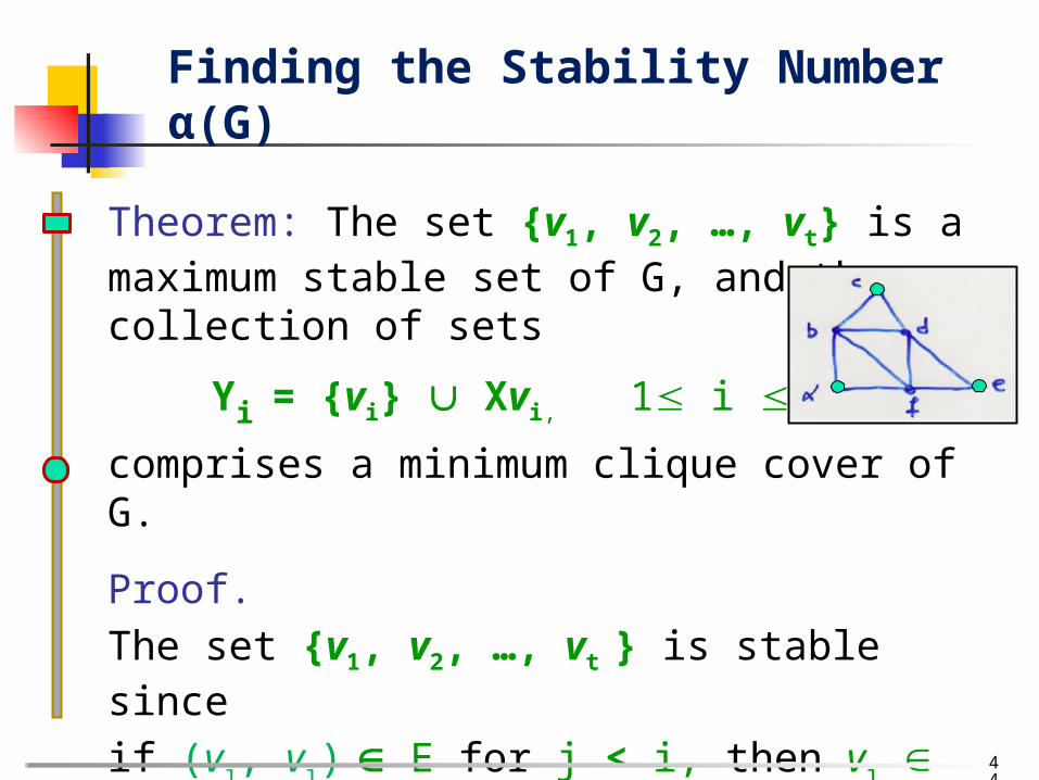
Theorem: The set {v1, v2, …, vt} is a maximum stable set of G, and the collection of sets

Yi = {vi} Xvi, 1 i t,

comprises a minimum clique cover of G.

Proof.

The set {v1, v2, …, vt } is stable since

if (vj, vi) E for j < i, then vi Xvj which cannot be.

Thus, α(G) t.


44

On the other hand, each of the sets Yi = {vi} Xvi

is a clique, and so {Y1, …, Yt} is a clique cover of G. Thus, α(G) = κ(G) = t.

We have produced the desired

maximum stable set and minimum clique cover.


45

Vertex Separators

Characterizations

46


Definition: A subset S of vertices is called a

Vertex Separator for nonadjacent vertices a, b

or, equivalently, a-b separator,

if in graph GV-S vertices a and b are in different connected components.

If no proper subset of S in an a-b separator, S is called

Minimal Vertex Separator.

Characterizing Triangulated Graphs

47

Example 1:

The set {y, z} is a minimal vertex separator for

p and q.

p

xy

q z

r


48

Example 2:

The set {x, y, z} is a minimal vertex separator for

p and r (p-r separator).

.

x


z

yq

r

p

49

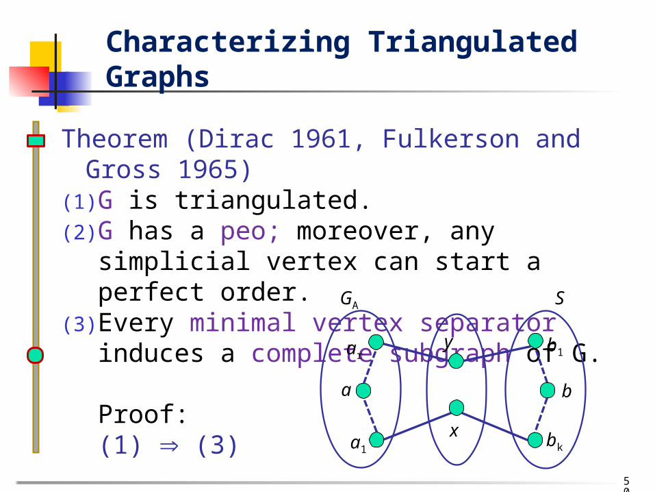
Theorem (Dirac 1961, Fulkerson and Gross 1965)(1) G is triangulated.(2) G has a peo; moreover, any simplicial vertex can

start a perfect order.(3) Every minimal vertex separator induces a complete

subgraph of G.

Proof:(1) (3)


GA S GB

b1

bka1

ar

a b

y

x

50

Let S be an a-b separator.

We will denote GA, GB

the connected components of GV-S containing a, b.

Since S is minimal, every vertex xS is a neighbor of a vertex in A and a vertex in B.

For any x,y S , minimal paths

[x,a1,…,ar,y] (ai A) and [x,bk,….,b1,y] (bi B)


GA S GB

b1

bka1

ar

a b

y

x

51

Since

[x, a1, …ar, y, b1, …., bk, x]

is a simple cycle of length

l 4, it contains a chord.

For every i, j aibjE, (S is a-b separate)

and also aiajE, bibjE (by the minimality of

the paths)

Thus, x y E.


GA S GB

b1

bka1

ar

a b

y

x

52

(3) (1) Suppose every minimal separator S is a clique

Let [v1,v2,….,vk,v1] be a chordless cycle.

v1 and v3 are nonadjacent.

Any minimal v1-v3 separator S1,3

contains v2 and at least one of v4,v5,……,vk.

But vertices v2,vi (i = 4, 5, …, k) are nonadjacent

S1,3 does not induce a clique.


vk

v1

v2

v3

v4

v5

53

The chordal graphs are exactly the intersection graphs of subtrees of trees.

That is, for a tree T and subtrees T1, T2, …, Tn

of T there is a graph G:

- its nodes correspond to subtrees T1, T2, …, Tn, and

- two nodes are adjacent if the corresponding subtrees share a node of T.

A characterization of Chordal Graphs

54

Example:

F

G B

D C

A

E

H H

D

F

C

A B

E

G


55

The graphs arising in this way are exactly the chordal graphs, and interval graphs arise when the tree T happens to be a simple path.


56

Theorem: Let G be a graph. The following statements are equivalent.

(i) G is an interval graph.

(ii) G contains no C4 and Ğ is a comparability graph.

(iii) The maximal cliques of G can be linearly ordered

such that, for every vertex x of G the maximal

cliques containing vertex x occur consecutively.

Interval Graphs

57

We have showed two main graph properties:

Chordal: if every cycle of length l > 3 has a chord.

Comparability: if we can assign directions to

edges of G so that the resulting

digraph G΄ is transitive.

Simple Elimination Scheme

58

Simple Elimination Scheme (SES):

A permutation σ = (v1, v2,…., vn) such that each

vi is simplicial in G - {v1, …, vi-1}, and

the neighborhoods of the vertices adjacent to vi

in G - {v1, …, vi-1} form a total order with respect to set containment.

or, Simple Elimination Ordering (SEO)


59

Example:

σ = (13,14,15,16,17,18,11,12,8,9,10,7,5,3,6,2,4,1)


60

If G is a chordal comparability graph, we will show that the following algorithm (Cardinality LexBFS) constructs a SEO.

The Cardinality LexBFS or CLexBFS is a modification of LexBFS that always prefers a vertex with largest possible degree.

We note that the reason we need CLexBFS is that it guarantees that if N(v) is proper subset of N(w), vertex v comes before w in the scheme.


61

Algorithm CLexBFS

1. for each vertex x in V(G) do • Compute the deg(x);• Initialize label(x) (); position(x) undefined;

2. for k n down to 1 do • Let S be the set of unpositioned vertices with largest

labels;• Let x be a vertex in S with largest degree;• Set σ(k) x; set label(x) k;• For each unpositioned vertex yadj(x) do

o append k to the label of y;


62

Example:

σ = (13,14,15,16,17,18,11,12,8,9,10,7,5,3,6,2,4,1)


63

Theorem: Given a chordal comparability graph, the CLBFS algorithm constructs a SES (or, SEO).

See: Borie, Spinrad, “Construction of a simple elimination scheme for a chordal comparability graph in linear time”, DAM 91(1999) 287-292.


64

Comparability Graphs

Properties & Algorithms

65


A graph G = (V, E) is a comparability graph if there exists an orientation (V, F) of G satisfying

F ∩ F-1 = Ø, F + F-1 = E, F2 F

where F2 = {ac | ab, bc F for some vertex b}


66

Define the binary relation Γ on the edges of an undirected graph G = (V, E) as follows:

ab Γ a’ b’ iff either a = a’ and b b’ E or b = b’ and a a’ E.

Edges ab, cd are in the same implication class

iff there exists a Γ-chain from ab to cd; ab Γ* cd,

that is

ab = a0b0 Γ a1b1 Γ … Γ akbk = cd


67

Example:

A = {ab, cb, cd, cf, ef, bf, A1={ab} ba, bc, dc, fc, fe, fb} A2={cd}

A3={ac, ad, ae} A4={bc, bd, be} A = Â = AA-1 A A-1 = Ø


68

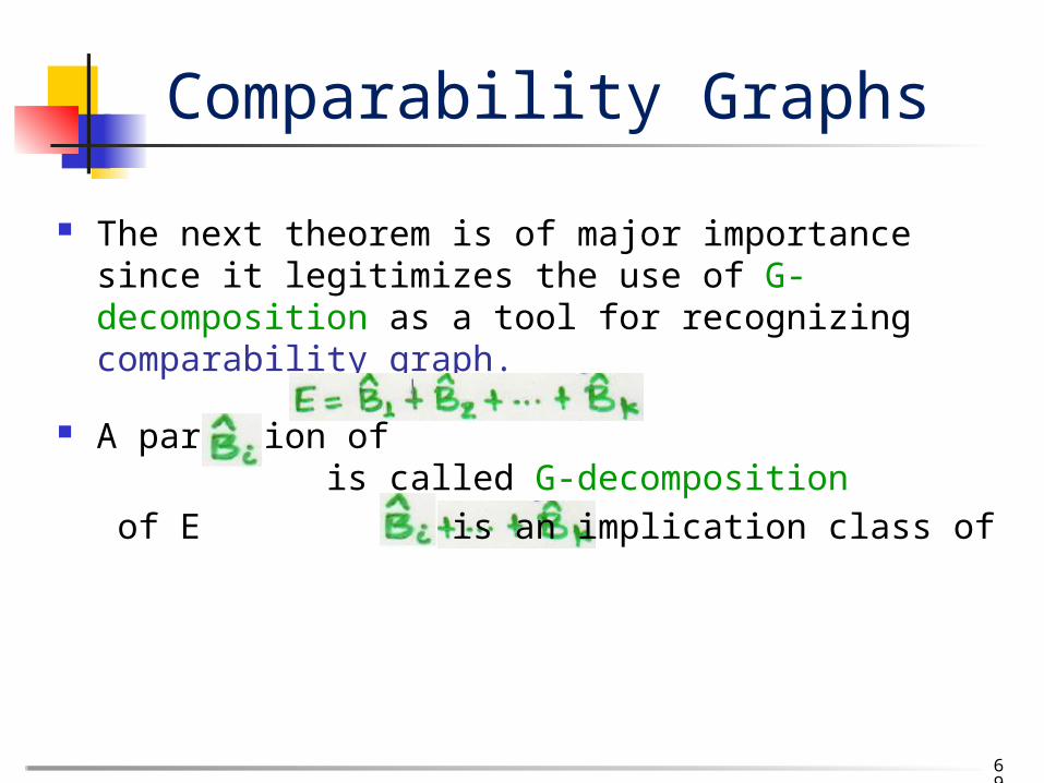
The next theorem is of major importance since it legitimizes the use of G-decomposition as a tool for recognizing comparability graph.

A partition of is called G-decomposition

of E if is an implication class of


69

Algorithm: Decomposition_Algorithm1. Initialize: i 1; Ei E; F Ø;

2. Arbitrarily pick an edge xiyi Ei ;

3. Enumerate the implication class Bi of E;if Bi∩Bi

-1 = Ø then add Bi to F;else “G is not comparability graph”; STOP;

4. Define: Ei+1 Ei - ;

5. if Ei+1= Ø then k i; output F; STOP;

else i i+1; goto 2;


70

Moreover, when these conditions hold, B1 + B2 + … + Bk is a transitive orientation of E.

71


Decomposition scheme [ac, bc, dc]

Theorem(TRO): Let be a

G-decomposition of G = (V, E). The following statements are equivalent:

(i) G = (V, E) is a comparability graph;

(ii) A A-1 = Ø for all implication classes A of E;

(iii) Bi Bi-1 = Ø for i =1, 2, ……, k;

(iv) every “circuit” of edges v1v2, v2v3,…, vqv1 E, such that vq-1v1, vqv2, vi-1vi+1 E

(for i = 2, 3,…., q-1) has even length.

72


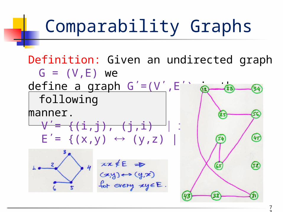
Definition: Given an undirected graph G = (V,E) wedefine a graph G΄=(V΄,E΄) in the followingmanner. V΄= {(i,j), (j,i) i, j V} E΄= {(x,y) (y,z) | xz E}

Example:

73


Theorem: (Ghouilla-Houri, 1962) The followingclaims are equivalent: 1. The graph G is a comparability graph2. The graph G΄ is bipartite

Proof: We will use GH characterization (Any oddcycle contains a short-chord).The vertices of a cycle in G΄correspond to adjacentedges in G (with common vertex), which induce a cycle in G with no chords.Thus, G΄ is bipartite G is a comparability graph.

74


Coloring

Maximum Weighted Clique

75


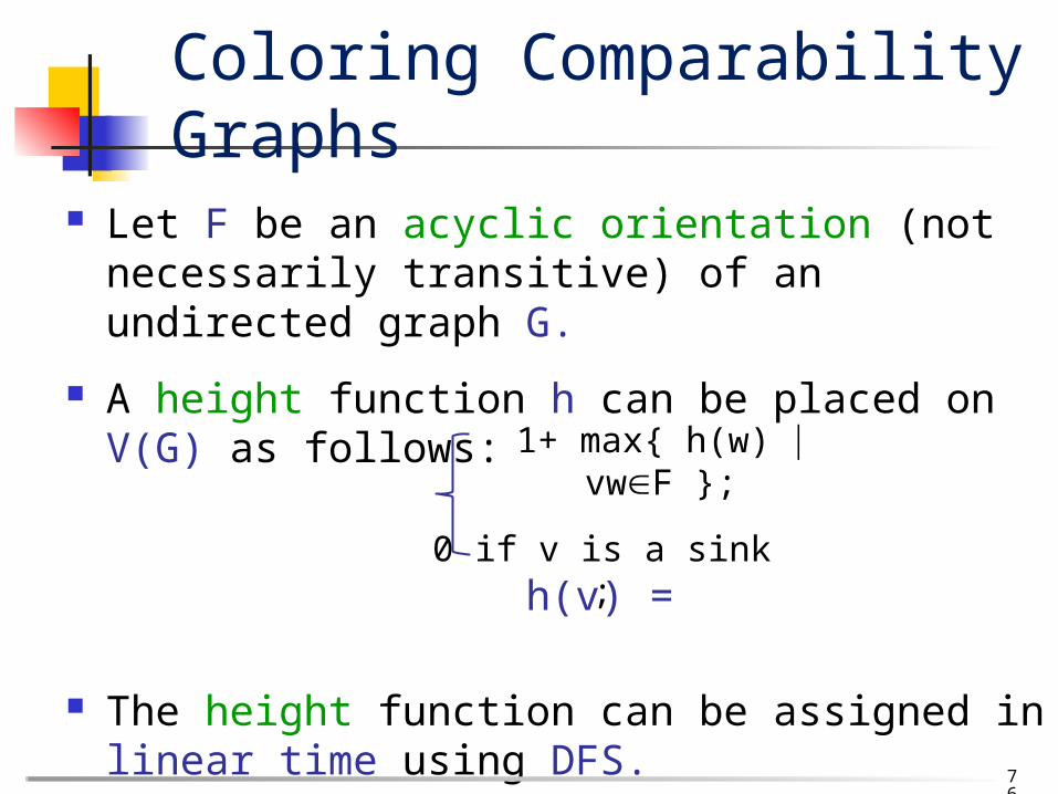
Let F be an acyclic orientation (not necessarily transitive) of an undirected graph G.

A height function h can be placed on V(G) as follows:

h(v) =

The height function can be assigned in linear time using DFS.

Coloring Comparability Graphs

1+ max{ h(w) vwF };

0 if v is a sink ;

76

The function h is always a proper vertex coloring of G, but it is not necessarily a minimum coloring.

#colors = #vertices in the longest path of F = 1+ max {h(v) vV}

The function h is a minimum coloring if F happens to be transitive.

77


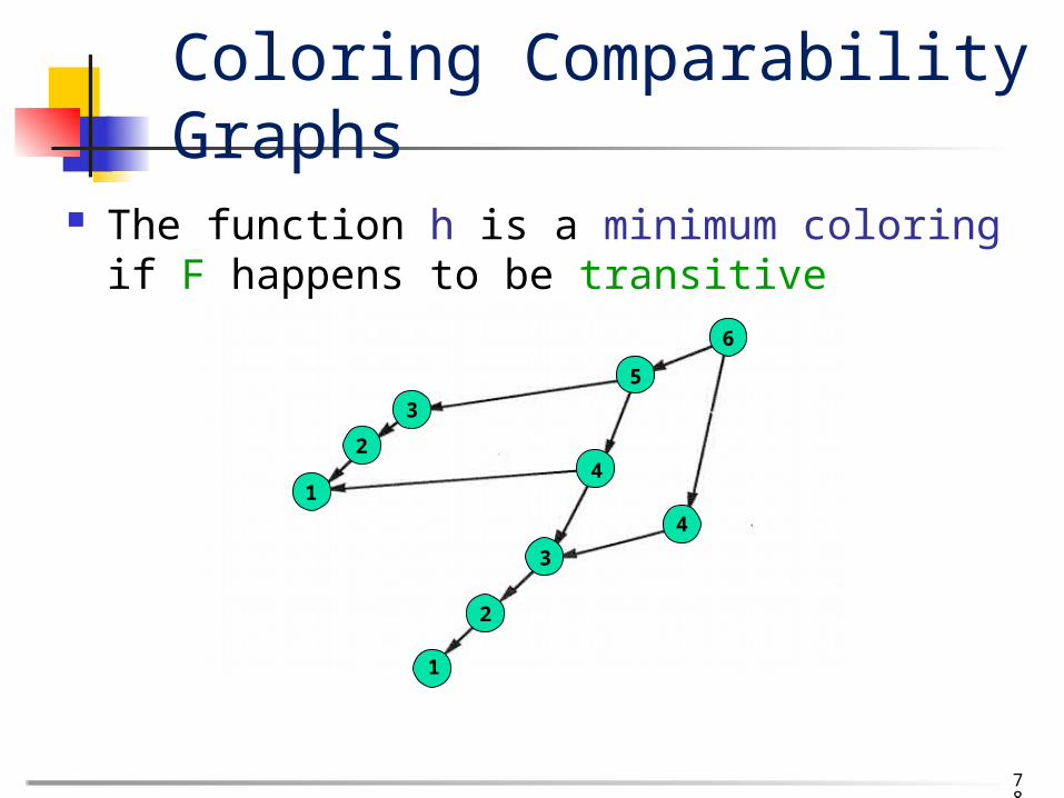
The function h is a minimum coloring if F happens to be transitive


78

1

2

3

1

2

3

4

5

4

6

Suppose that G is a comparability graph, and let F be a transitive orientation of G.

79


In such a case, every path in F corresponds to a clique of G because of transitivity.

80


Thus, the height function will yield a coloring of G which uses exactly ω(G) colors, which is the best possible.

81


1

2

3

1

2

3

4

5

4

6

Moreover, since being a comparability graph is a hereditary property, we find that ω(GA) = χ(GA) for all induced subgraphs GA of G.

This proves: Every comparability graph is a perfect graph.

82


In general the maximum weighted clique problem is NP-complete, but when restricted to comparability graphs it becomes tractable.

Algorithm MWClique

Input: A transitive orientation F of a comparability graph G = (V, E) and a weight function w

defined on V.

Output: A clique C of G whose weight is max.

Maximum Weighted clique

83

Method: We use a modification of the height calculation technique (DFS).

To each vertex v we associate its cumulative weight W(v) = the weight of the heaviest path from v to some sink.

A pointer is assigned to v designating its successor on that heaviest path.

84

Maximum Weighted clique

Αλγοριθμική Θεωρία Γραφημάτων

Documents

e abcde

triangulated property

triangulated graph property

triangulated graphsdirac

triangulated graphslet

triangulated graphsfulkerson

triangulated graphsnote

b abde