© 2013 ashesh sharma - university of...
TRANSCRIPT
1
MICROMECHANICS OF COMPOSITES USING A TWO-PARAMETER MODEL AND RESPONSE SURFACE PREDICTION OF ITS PROPERTIES
By
ASHESH SHARMA
A THESIS PRESENTED TO THE GRADUATE SCHOOL OF THE UNIVERSITY OF FLORIDA IN PARTIAL FULFILLMENT
OF THE REQUIREMENTS FOR THE DEGREE OF MASTER OF SCIENCE
UNIVERSITY OF FLORIDA
2013

2
© 2013 Ashesh Sharma

3
To my parents, thank you both for supporting me in every possible way to help me achieve my goals and fulfill my dreams.

4
ACKNOWLEDGMENTS
Firstly, I would like to thank my parents for their encouragement, blessings and
never ending support which has helped me achieve one of the most cherished dreams
of my life, i.e. to study in the USA which has allowed me to participate in research work
of such a magnitude. I would like to thank Dr. Bhavani V. Sankar for taking me on as a
Master’s student and giving me a chance to work on this wonderful project.
I would also like to thank the members of my supervisory committee, Dr. Raphael
T. Hatka and Dr. Ashok Kumar. I am grateful for their willingness to serve on my
committee, and for constructive criticism they have provided.
I would also like to thank my lab colleague, Sayan Banarjee for providing
valuable guidance at many stages of this research work. A very special thanks to Dr.
Raphael Haftka for being ever so patient while helping me out with doubts concerning
surrogate modeling over my progress during this project. It has truly been wonderful
working with everyone.
5
TABLE OF CONTENTS
Page
ACKNOWLEDGMENTS .................................................................................................. 4
LIST OF TABLES ............................................................................................................ 7
LIST OF FIGURES .......................................................................................................... 8
ABSTRACT ................................................................................................................... 10
CHAPTER
1 INTRODUCTION .................................................................................................... 11
1.1 Scope of Work .................................................................................................. 11 1.2 Thesis Outline ................................................................................................... 12
2 BACKGROUND AND LITERATURE REVIEW ....................................................... 13
2.1 History of Micromechanics ................................................................................ 13 2.2.1 Rule of Mixtures – Voigt and Reuss Models .......................................... 15
2.2.2 Eshelby’s Solution (1957) ...................................................................... 17 2.2.3 Self-Consistent Theory (1965) and Halpin-Tsai Equations (1969) ........ 20 2.2.4 Mori-Tanaka Method (1973) .................................................................. 23
2.2.5 Method of Cells (1989) .......................................................................... 24
2.3 Use of Finite Element Based Analysis .............................................................. 25 2.4 Introduction to Surrogate Modeling ................................................................... 26
3 TWO-PARAMETER BASED APPROACH USING MICROMECHANICS ............... 30
3.1 Concept of Homogenization .............................................................................. 30 3.1.1 Concept of Average Stresses ................................................................ 31
3.1.2 Concept of Average Strains ................................................................... 32 3.2 Transverse Isotropy .......................................................................................... 33 3.3 The Two-Parameter Model ............................................................................... 39
3.3.1 Finite element analysis of representative volume element .................... 45 3.3.2 Completing the T-matrix ........................................................................ 55
4 RESPONSE SURFACE PREDICTION OF THE PARAMETERS – T22 AND T32 .... 57
4.1 Surrogate Modeling Using Polynomial Response Surfaces .............................. 57 4.2 Constructing the Response Surface ................................................................. 61
4.2.1 Selection of Variables And Generation of Design Points ....................... 61 4.2.2 Constructing and Choosing an Accurate Response Surface ................. 63
4.3 Result Analysis ................................................................................................. 65
4.3.1 Adopting a Reliable Estimate for the Halpin-Tsai Parameter, ............. 66 4.3.2 Result Analysis apropos T-300 Epoxy ................................................... 68

6
4.3.3 Result Analysis apropos Graphite Epoxy .............................................. 69 4.3.4 Result Analysis apropos Kevlar Epoxy .................................................. 70 4.3.5 Result Analysis apropos S-glass Epoxy ................................................ 71
4.3.6 Result Analysis apropos E-glass Epoxy ................................................ 72 4.3.7 Result Analysis apropos Boron Epoxy ................................................... 73
5 PREDICTING THE LONGITUDNAL SHEAR MODULUS ....................................... 74
5.1 Extracting Using Abaqus ........................................................................... 74 5.1.1 Analysis of the Hexagonal Finite Element Model .................................. 74
5.1.2 Using Displacement along Z-axis to Calculate ............................... 76
5.2 Predicting Using Polynomial Response Surface ....................................... 81
6 CONCLUSION ........................................................................................................ 83
6.1 Summary .......................................................................................................... 83 6.2 Future Scope of Work ....................................................................................... 85
APPENDIX: RESPONSE SURFACE COEFFICENTS .................................................. 86
A.1 For The Prediction Of And ................................................................. 86
A.2 For The Prediction Of ............................................................................... 88
REFERENCES .............................................................................................................. 89
BIOGRAPHICAL SKETCH ............................................................................................ 93
7
LIST OF TABLES
Table page
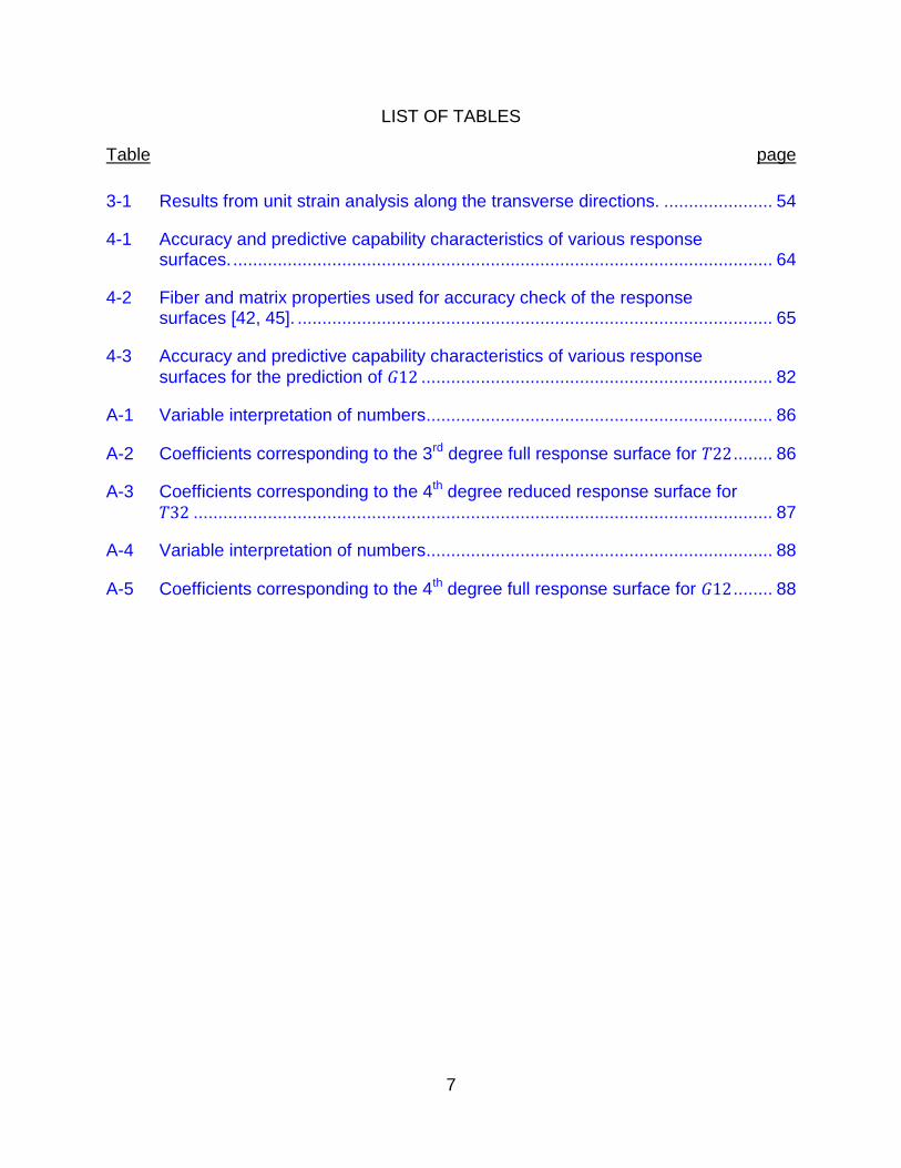
3-1 Results from unit strain analysis along the transverse directions. ...................... 54
4-1 Accuracy and predictive capability characteristics of various response surfaces. ............................................................................................................. 64
4-2 Fiber and matrix properties used for accuracy check of the response surfaces [42, 45]. ................................................................................................ 65
4-3 Accuracy and predictive capability characteristics of various response
surfaces for the prediction of ....................................................................... 82
A-1 Variable interpretation of numbers ...................................................................... 86
A-2 Coefficients corresponding to the 3rd degree full response surface for ........ 86
A-3 Coefficients corresponding to the 4th degree reduced response surface for
..................................................................................................................... 87
A-4 Variable interpretation of numbers ...................................................................... 88
A-5 Coefficients corresponding to the 4th degree full response surface for ........ 88

8
LIST OF FIGURES
Figure page
2-1 Ellipsoidal inclusion problem and Eshelby’s decomposition associated with the problem......................................................................................................... 19
2-2 Arrangement of fiber and matrix ......................................................................... 22
2-3 Original Method of Cells model with representative volume element (RVE) consisting of 1 fiber sub-cell and 3 matrix sub-cells. ........................................... 25
2-4 A function f(x) trying to mimic the underlying behavior corresponding to a set of selected data points. The space between two data points may or may not reflect the true nature of the process that is being modeled. .............................. 28
3-1 Cross-section of a hexagonal unit cell lying in the 2-3 plane, before and after a 60 degree rotation about the longitudinal axis. ................................................ 36
3-2 A unidirectional fiber surrounded by matrix ........................................................ 40
3-3 Representative volume elements for composites ............................................... 46
3-4 Axis configuration ............................................................................................... 47
3-5 1/4th representative volume element ................................................................... 49
3-6 Boundary conditions for RVE analysis ................................................................ 50
3-7 Schematic of the procedure followed to obtain , , and . .............. 52
3-8 Hexagonal RVE model undergoing unit strain deformation ................................ 53
4-1 Variation of with the fiber volume fraction, in models with isotropic fibers ....... 67
4-2 Comparison between the response surface, and rule of mixtures with respect to finite element analysis of T-300 epoxy using Abaqus ..................................... 68
4-3 Comparison between the response surface, and rule of mixtures with respect to finite element analysis of Graphite epoxy using Abaqus ................................ 69
4-4 Comparison between the response surface, and rule of mixtures with respect to finite element analysis of Kevlar epoxy using Abaqus .................................... 70
4-5 Comparison between the response surface, and rule of mixtures with respect to finite element analysis of S-glass epoxy using Abaqus .................................. 71

9
4-6 Comparison between the response surface, and rule of mixtures with respect to finite element analysis of E-glass epoxy using Abaqus .................................. 72
4-7 Comparison between the response surface, and rule of mixtures with respect to finite element analysis of Boron epoxy using Abaqus ..................................... 73
5-1 Boundary conditions for shear strain analysis. ................................................... 75
5-2 Hexagonal RVE model undergoing unit shear strain deformation in the x-z plane. .................................................................................................................. 76
5-4 Quadrilateral equivalent of a triangular reference element. ................................ 79
5-5 Step by step schematic, for calculating the longitudinal shear modulus of the composite using the displacement of the finite element model along the z-axis. .................................................................................................................... 80
5-6 Variation of fiber longitudinal shear modulus with respect to the volume fiber ratio ........................................................................................................ 81

10
Abstract of Thesis Presented to the Graduate School of the University of Florida in Partial Fulfillment of the
Requirements for the Master of Science
MICROMECHANICS OF COMPOSITES USING A TWO-PARAMETER MODEL AND RESPONSE SURFACE PREDICTION OF ITS PROPERTIES
By
Ashesh Sharma
May 2013
Chair: Bhavani V. Sankar Major: Mechanical Engineering
A novel method involving the use of micro-mechanical analysis to predict elastic
constants of a unidirectional fiber-reinforced composite is proposed. The method
revolves around a model called the two-parameter model. The model, similar to
Eshelby’s theory for an ellipsoidal inclusion, is shown to be efficient for the calculation of
four out of five elastic constants of a transversely isotropic composite material. The two
parameters are obtained by performing one micromechanical analysis of the composite
unit cell along any of its transverse directions. Although the theory is shown to work for
both, square and hexagonal unit cells, the thesis focuses on hexagonal unit cells. The
method involves construction of surrogate models that act as response surface for the
prediction of the two parameters corresponding to any fiber-reinforced composite design
that uses a transversely isotropic fiber and an isotropic matrix. The fifth elastic constant,
longitudinal shear modulus is predicted using a separate response surface based on
finite element simulations in Abaqus. The results indicate that the two parameter model
in conjunction with the response surface makes accurate prediction of composite elastic
constants. Based on the results modified Halpin-Tsai equations are proposed for
transverse properties of composites with hexagonal unit-cells.
11
CHAPTER 1 INTRODUCTION
1.1 Scope of Work
Micromechanics has been a widely adopted approach for the prediction of effective
properties of a composite material. Most methods in micromechanics of materials are
based on continuum mechanics rather than on atomistic approaches such as molecular
dynamics. For more than a century, researchers have made use of continuum
mechanics to come up with various mathematical expressions including rules of
mixtures (Voigt (1887) and Reuss (1929)), and mean field methods (e.g. Eshelby(1957))
leading to the derivation of semi-empirical formulae (Halpin and Tsai (1969)), as models
for the calculation of approximate effective properties.
One problem with semi-empirical formulae is that they are not based on
observations and experiments, but on theory combined with analytics. While these
models have been shown to be more or less accurate in most of the cases, a need for
an entirely empirical expression is felt such as that of a surrogate model, which is
constructed solely on the basis of data collected using simulations. One such attempt
has been made through the medium of the research presented in this thesis. A less
expensive way of developing such expressions is through the construction of polynomial
response surfaces based on a micromechanical model, where the surrogate models
have been built using numerous data points obtained after performing finite element
based analysis of designs corresponding to each data point.
The essence of this approach is a two-parameter model which is essentially a
mean field method, similar to Eshelby's solution for an ellipsoidal inclusion in an infinite
solid. Although the two-parameter model is found to be efficient in predicting the
12
effective longitudinal moduli of composites, this model is more relevant for the prediction
of effective transverse moduli and is shown to be slightly more accurate than the Halpin-
Tsai equations.
1.2 Thesis Outline
The primary objective of the dissertation was to come up with a set of expressions
that will help in the accurate prediction of the effective composite properties (particularly
the elastic moduli) of a unidirectional fiber-reinforced composite. Composites with only
transversely isotropic fiber or completely isotropic fiber, combined with an isotropic
matrix only, have been taken into account.
A significant part of coming up with these expressions is the derivation of the two-
parameter model, which is essentially a micromechanical model based on Eshelby’s
theory for inhomogeneous material. The model, although valid for both square and
hexagonal unit cells, is implemented using a response surface, for only hexagonal unit
cells. The elastic constants predicted using the two-parameter model are , , ,
.A separate response surface is constructed for the prediction of the longitudinal
shear modulus, .
All the response surfaces were constructed using the surrogate toolbox developed
by Felipe A. C.Viana [2].

13
CHAPTER 2 BACKGROUND AND LITERATURE REVIEW
2.1 History of Micromechanics
Composite materials - are engineered or naturally occurring materials made from
two or more constituent materials with significantly different physical or chemical
properties which remain separate and distinct within the finished structure. Engineers
have constantly been exploiting the field of composites as a source for stronger and
stiffer, yet lighter materials. Other properties that can be improved by forming a
composite material include thermal conductivity, fatigue life, wear resistance,
temperature resistance and thermal properties such as thermal conductivity and
coefficient of thermal expansion, etc [34]. The primary objective here is to develop a
material that has only the characteristics which are needed to perform the design task in
question.
Composite materials are usually orthotropic or transversely isotropic [3]. This
property makes it difficult for the analyst to analyze their behavior which is necessary to
the design process of any structure involving the materials. The properties of the
composite itself are not known, especially if the constituent materials themselves have
been changed. Therefore, it is required, that extensive testing of the composite is
performed before deeming it usable. That is, the knowledge of the nature of
directionality (isotropic or anisotropic) of the composite is not enough. In addition, an
appropriate failure criteria along with a numerical method (such as the Finite Element
Method) to solve the boundary value problem should be known for the complete
analysis of a laminate of the concerned composite material.
14
Generally, this heterogeneous nature of composite materials is studied from two
points of view – macromechanics and micromechanics. Many composite analyses are
performed using macromechanical analysis, wherein material is assumed to be
homogenous and the effects of the constituent materials are treated as averaged
apparent macroscopic properties of the composite material. However, the true nature of
a composite material is that of a randomly space anisotropic material (called the fiber) in
an isotropic medium (called the matrix). In contrast to macromechanics,
micromechanics examine the interaction of the constituent materials at a microscopic
scale, and study their effect on the overall properties of the composite. Consequently,
investigation of micromechanics is an approach based solely on the constituent
materials of a composite and how various proportions and arrangements of the
constituent materials may help in achieving the desired properties. In doing so, a
micromechanical approach may provide a better insight into the interactions between
the fiber and the matrix, thus providing with a more accurate model for analyzing the
behavior of the composite. In some instances the constituents include the interface
between the fiber and the matrix, where the transition of properties occur. This interface
(at times also termed as interphase) plays a crucial role in the behavior of the
composite.
An important advantage posed by a micromechanical model over a
macromechanical model is the ability of micromechanics to capture the physical
deformation and damage at a more fundamental scale. This allows for easier grasping
of in-situ multi-axial stress and strain rates. Not to mention, micromechanics utilizes
simpler isotropic constituent constitutive models and failure criteria [4]. It is important to

15
note that failure tends to occur mostly at the micromechanical level, making it difficult to
be captured at the macroscopic level. Properties that can be predicted using
micromechanics include thermo-elastic constants, viscoelastic properties, strength
properties, yield function, fracture toughness, thermal conductivities and
electromagnetic properties [5].
It should be pointed out that micromechanics is still an approximation of any real
composite model, most significantly the approximation of the fiber geometry within a
composite. Over the next few sub-sections, various micromechanical models developed
over the years are discussed. Excluding the rule of mixtures (2.2.1), all the analytical
approaches described in the following sub-sections are mean field methods. By
definition, mean field methods assume that the stress and strain field, in the matrix and
the fiber, are adequately represented by their volume-averaged values, though they
differ in the way they account for the elastic interaction between the phases. These
methods were later extended to include plasticity [14].
2.2.1 Rule of Mixtures – Voigt and Reuss Models
Generally, the “rule of mixture” expression for some scalar effective physical
property Ψ of a two-phase composite takes the form,
[ ( )
( )( ) ]
(2-1)
where(i) and (m) denote inhomogeneities (mostly fiber) and matrix respectively. The
exponent β is chosen so as to draw a good fit to the data obtained from experiments [6].
The Voigt model (1887) assumes constant strain throughout the composite (iso-
strain model) [7]. The effective composite stiffness is calculated as a combination of the
individual fiber and matrix stiffness weighted by their respective volume fractions. The

16
result, thus, is a rule of mixtures formulation for the stiffness components of a composite
(β = 1 in Eq. 2-1).
[ [ ] ( )[ ]] (2-2)
Here is the equivalent stiffness for the composite. and are the stiffness
components for the fiber and matrix elements respectively. is the fiber-volume ratio
for the composite material.
Reuss (1929) proposed a rule of mixture model where stress was assumed to be
constant throughout the composite (iso-stress model) [8]. This model calculates the
effective composite compliance as a combination of the individual fiber and matrix
compliance weighted by their respective volume fractions. The result, thus, is a rule of
mixtures formulation for the compliance components of a composite (β = -1 in Eq. 2-1).
[ [ ] ( )[ ]] (2-3)
Here is the equivalent compliance for the composite. and are the compliance
components for the fiber and matrix elements respectively.
It is suggested that Voigt-type expressions (Eq. 2.2), correspond to "full strain
coupling of the phases (springs in parallel, arithmetic averages)"whereas, the Reuss-
type expressions (Eq. 2.3) correspond to "full stress coupling of the phases (“springs in
series, harmonic averages)" [6]. The practical use of these models however, depends
on the microtopology and material properties of the composite in discussion. The
models are closely related to the Hill bounds [9], with the Voigt model providing the
upper bound and the Reuss model providing the lower bound [10].There are a few
cases where the prediction of the Voigt and Reuss models is known to lie outside the
Hashin–Shtrikman bounds. Hashin–Shtrikman provided bounds on the elastic moduli

17
and tensors of transversally isotropic composites [13] (reinforced by aligned continuous
fibers) and isotropic composites [11] (reinforced by randomly positioned particles).
Another approach closely related to the rule of mixtures is the Vanishing Fiber
Diameter Model (VFD). Developed by Dvorak and Bahei-el-din in 1982, the model
depicts combination of average stress and strain assumptions visualized as each fiber
having a vanishing diameter yet finite volume within a matrix [6, 12].
2.2.2 Eshelby’s Solution (1957)
Eshelby’s solution for the analysis of a heterogeneous material has been of great
usefulness in the field of continuum micromechanics.
A solution was first derived for “The Transformation Problem”. The problem is
defined using a region (referred to as the ‘inclusion) in an infinite homogeneous
isotropic elastic medium. The inclusion undergoes deformation which, if not constrained
by the surroundings (referred to as the matrix), would be equal to an arbitrarily applied
homogeneous strain. The question posed by this problem, requires the determination of
the elastic state of the inclusion and the matrix. Eshelby suggested that the problem
could be solved by removing the inclusion from the infinite medium and allowing it to
deform. Now, surface tractions were applied to bring the inclusion back to its original
form, after which the inclusion was placed back in the medium. Although the matrix is
now stress free, the inclusion is under a state of constant stress. The surface tractions
applied to the inclusion will manifest as a layer of body forces spread over the interface
between the inclusion and the matrix [5]. Since these forces were not present in the
original problem, they have to be removed by applying equal but opposite body forces,
which will induce stresses in the matrix as well as the inclusion. Since the matrix and
inclusion are made of the same material, this problem could be solved using the
18
stresses due to a point force inside an infinite medium as the Green’s function. The
solution will yield the correct stresses for the matrix, but for the inclusion, the uniform
state of compressive stresses should be added to complete the solution. Up until this
point, nothing was assumed regarding the shape of the inclusion. However, if an
ellipsoidal shape is assumed, it was proved that the stress within the inclusion is
uniform [15].
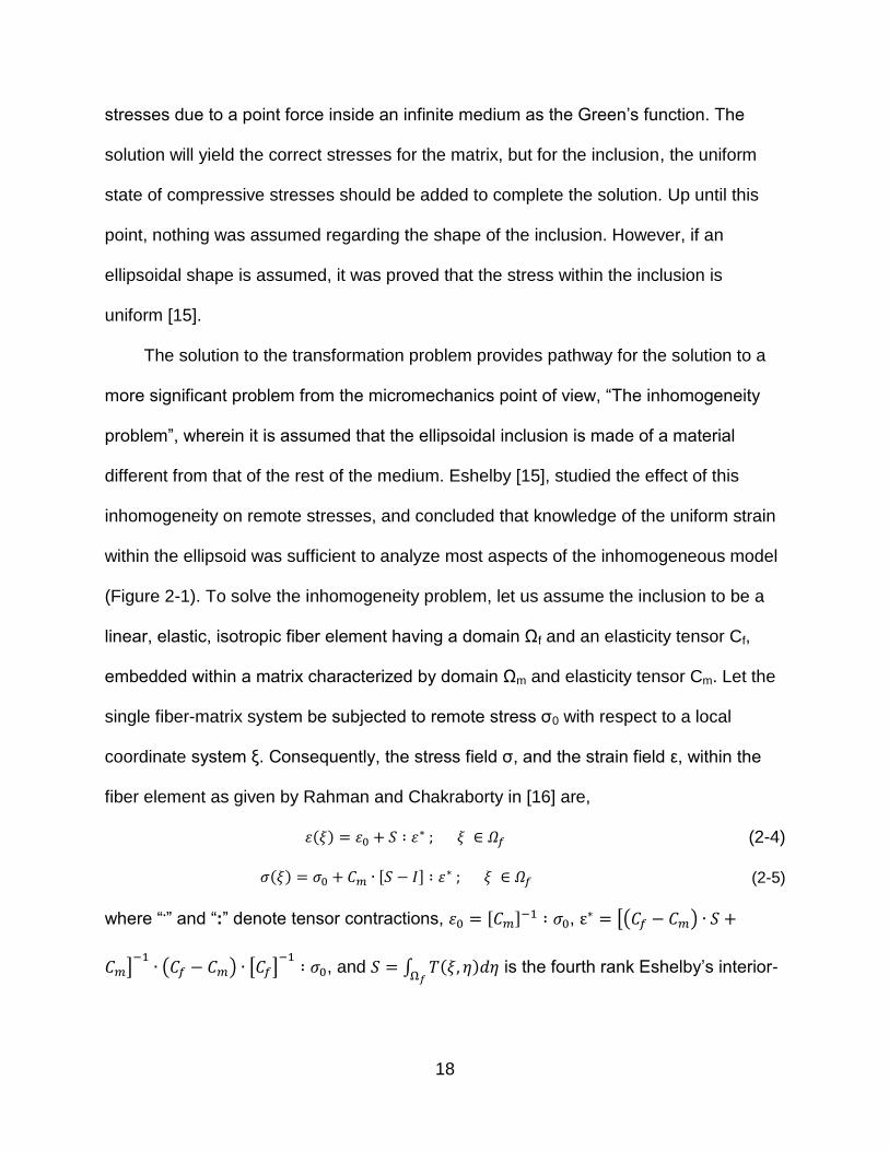
The solution to the transformation problem provides pathway for the solution to a
more significant problem from the micromechanics point of view, “The inhomogeneity
problem”, wherein it is assumed that the ellipsoidal inclusion is made of a material
different from that of the rest of the medium. Eshelby [15], studied the effect of this
inhomogeneity on remote stresses, and concluded that knowledge of the uniform strain
within the ellipsoid was sufficient to analyze most aspects of the inhomogeneous model
(Figure 2-1). To solve the inhomogeneity problem, let us assume the inclusion to be a
linear, elastic, isotropic fiber element having a domain Ωf and an elasticity tensor Cf,
embedded within a matrix characterized by domain Ωm and elasticity tensor Cm. Let the
single fiber-matrix system be subjected to remote stress σ0 with respect to a local
coordinate system ξ. Consequently, the stress field σ, and the strain field ε, within the
fiber element as given by Rahman and Chakraborty in [16] are,
( ) (2-4)
( ) [ ] (2-5)
where “.” and “:” denote tensor contractions, [ ] , [( )
]
( ) [ ]
, and ∫ ( )
is the fourth rank Eshelby’s interior-

19
point tensor. ( ) is the fourth ranked Green’s function tensor that depends on the
shear modulus and the Poisson’s ratio of the matrix.
=
+
Ωm,Cm
Ωf,Cf
σ0
Ωf,Cf,ε*
Ωm,Cm
σ0
Figure 2-1. Ellipsoidal inclusion problem and Eshelby’s decomposition associated with the problem.
20
It is to be mentioned here that the Eshelby model is valid only for a single inclusion
in an infinite medium. Hence, if more than one inclusion is taken into account, it is
important to make sure that the inclusions are far apart. The self-consistent method
developed by Hill (2.2.3) and the Mori-Tanaka method (2.2.4), are effective medium
theories based on Eshelby’s elasticity solution for inhomogeneities in an infinite
medium.
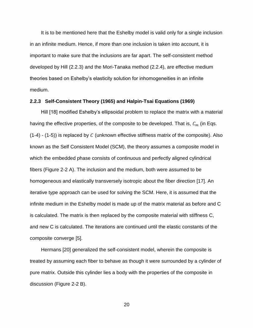
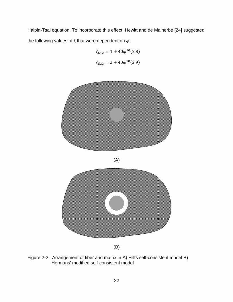
2.2.3 Self-Consistent Theory (1965) and Halpin-Tsai Equations (1969)
Hill [18] modified Eshelby’s ellipsoidal problem to replace the matrix with a material
having the effective properties, of the composite to be developed. That is, (in Eqs.
(1-4) - (1-5)) is replaced by (unknown effective stiffness matrix of the composite). Also
known as the Self Consistent Model (SCM), the theory assumes a composite model in
which the embedded phase consists of continuous and perfectly aligned cylindrical
fibers (Figure 2-2 A). The inclusion and the medium, both were assumed to be
homogeneous and elastically transversely isotropic about the fiber direction [17]. An
iterative type approach can be used for solving the SCM. Here, it is assumed that the
infinite medium in the Eshelby model is made up of the matrix material as before and C
is calculated. The matrix is then replaced by the composite material with stiffness C,
and new C is calculated. The iterations are continued until the elastic constants of the
composite converge [5].
Hermans [20] generalized the self-consistent model, wherein the composite is
treated by assuming each fiber to behave as though it were surrounded by a cylinder of
pure matrix. Outside this cylinder lies a body with the properties of the composite in
discussion (Figure 2-2 B).

21
Halpin and Tsai [19], used Hermans’ solution to generalize Hill’s self-consistent
model, abbreviating it to an approximate form that can be used to obtain the transverse
Young’s modulus, the longitudinal shear modulus and the transverse Poison's ratio
using the semi-empirical formula,
(2-6)
where,
(2-7)
Here, is an effective composite modulus, is the corresponding fiber modulus, is
the corresponding matrix modulus, is the fiber volume fraction, and is a measure of
the reinforcement geometry which is dependent on the loading conditions.
Equation (2-6) provides reasonable estimates for the equivalent longitudinal shear
modulus , the equivalent transverse Young's modulus and the equivalent
transverse Poison's ratio . Reliable estimates of have been obtained by comparison
of equations (2-6) and (2-7) with the numerical micromechanics solution employing
formal elasticity theory. Halpin and Tsai, found that the value , gave an excellent fit
to the finite difference elasticity solution of Adams and Doner [21] for of composite
model of square array with circular fibers. For the same material and fiber volume
fraction, a value of , was found to be in good agreement for [22]. The Halpin-
Tsai formula also claims to provide a good correlation with Foye's computations [23] for
hexagonal array of circular fibers with volume fiber fraction of up to 65%. However,
exact elasticity calculations predict the moduli to "rise faster with increasing volume
fraction of reinforcement above a volume fiber fraction of 0.70" [17] as compared to the
22
Halpin-Tsai equation. To incorporate this effect, Hewitt and de Malherbe [24] suggested
the following values of that were dependent on .
( )
( )
(A)
(B)
Figure 2-2. Arrangement of fiber and matrix in A) Hill's self-consistent model B) Hermans' modified self-consistent model

23
2.2.4 Mori-Tanaka Method (1973)
Until now, none of the methods discussed, take into account the interaction
between inhomogeneities. One way of introducing collective interactions amongst
inhomogeneities consists of approximating the stresses acting on an inhomogeneity,
which may be viewed as disturbance stresses (that are caused due to the presence of
other inhomogeneities) superimposed on the already present far field stress. Here
fourth order tensor relates average inclusion strain to average matrix strain and
approximately accounts for fiber interaction effects. An important feature of this model
was the consideration of internal elastic energy due to the presence of interaction
effects between the inclusions along with the presence of a free boundary. Mori and
Tanaka presented a method for calculating the average stress, within the matrix of a
material containing inclusions, with transformation strain. They showed that the average
stress in the matrix is uniform throughout the material and independent of the position of
the domain where the average treatment is carried out. They also proved that the actual
stress in the matrix is equal to the sum of the average stress and, the locally fluctuating
stress (disturbance stresses), the average of which was shown to vanish in the matrix
body of the composite [25].
Mori-Tanaka model describe composites consisting of aligned ellipsoidal
inhomogeneities embedded in a matrix, i.e., "inhomogeneous materials with a distinct
matrix-inclusion microtopology" [6]. Ponte Castaneda and Willis [26] showed that the
Mori-Tanaka method could be treated as a special case of the Hashin-Shtrikman
variational estimates [13] where the spatial arrangement of the inhomogeneities follows
an ellipsoidal distribution which has the same aspect ratio and orientation as that of the
inhomogeneities themselves, as portrayed in [6].

24
The Mori-Tanaka approach has been used in the development of a recently
created micromechanical model, the Bridging model [32]. The bridging model requires
the knowledge of only the constituent fiber and matrix properties along with the fiber
volume ratio of the composite. Here, a fourth-order tensor relates average fiber stress to
average matrix stress and thermal residual constituent stresses can be predicted.
2.2.5 Method of Cells (1989)
The method of cells is a micromechanical model developed by J. Aboudi [28],
which has been shown to accurately predict the overall behavior of various types of
composites from the knowledge of the constituent properties. This method explicitly
yields effective constitutive equations for the inelastic behavior of metal matrix
composites. The overall behavior of, inelastic multi-phase unidirectional fibrous
composites, predicted by the method of cells is portrayed in terms of - the effective
elastic moduli, effective coefficients of thermal expansion, effective thermal
conductivities and the effective stress-strain response in the inelastic region [29].
The inclusion geometry consists of "doubly-periodic array of fibers" [29] embedded
within the matrix with the unit cell further divided into four sub-cells, one for the fiber and
three for the matrix as shown in Figure 2-3. Being a mean field method, the effective
stiffness matrix is obtained by relating the average stresses to the average strains
inside the sub-cells, and consequently average over the complete volume of the unit
cell.
Consequently, Aboudi went on to propose a generalized formulation (Generalized
Method of Cells Model) wherein the repeating unit cell is subdivided into an arbitrary
number of sub-cells. The purpose of this generalization, was to extend the modeling
capability of the original method of cells to further include the thermo-mechanical

25
response of multi-phase metal matrix composites, modeling of variable fiber shapes,
analysis of different fiber arrays, modeling or porosities and damage, and modeling of
interfacial degradation [29]. This generalization of the original method of cells allowed
for micromechanical analysis of much more complicated periodic array of cells.
X2
X1
X3
Fiber elements Matrix
RVE
F
M M
M
Figure 2-3. Original Method of Cells model with representative volume element (RVE) consisting of 1 fiber sub-cell and 3 matrix sub-cells.
2.3 Use of Finite Element Based Analysis
The finite element method (FEM) is a numerical techniquefor finding approximate
solutions to partial differential equations and their systems, as well as integral equations
[33]. In simple terms, FEM is a method for dividing up a very complicated problem into
small elements that can be solved in relation to each other. With the onset of an era

26
dominated by computers, finite element based analysis has become one of the most
widely accepted approach for engineers, in the field of design.
Most micromechanical methods use periodic homogenization. That is, the
composite material is characterized by a periodic unit cell (or a representative volume
element). The overall elastic behavior of such a composite is now governed by the
behavior of an individual unit cell which can be described using a combination of
boundary conditions, stress fields and strain fields. Finite element formulations can
prove to be a very efficient tool in accurately capturing the mechanical behavior of such
heterogeneous materials. Thus, due to its high flexibility and efficiency, finite element
methods, at present are one of the most widely used numerical tool in the field of
continuum micromechanics.
The presented research was carried out using Abaqus/CAE, or "Complete Abaqus
Environment". It is a software application used for both, the modeling and analysis of
mechanical components and assemblies (pre-processing) and visualizing the finite
element analysis result. Abaqus provides the analyst with the ability to add to the
material and element libraries through the use of user sub-routines coded in FORTRAN.
For this research, a student edition of Abaqus was used, which limits the maximum
number of mesh nodes to 1000. This is the primary reason as to why only quarter of the
complete unit cell has been used for analysis.
2.4 Introduction to Surrogate Modeling
For many real world problems, a single simulation can take huge amounts of time,
thus increasing the overall cost of the design process. A cheaper way of going about
this process is by constructing approximation models, known as surrogate models. The
phenomenon of surrogate modeling can be explained as the process of developing a

27
continuous function f(x), (based on a set of carefully chosen design variables) when
only limited amount of data is available [30]. This function helps in filling the underlying
gaps between the simulated data points (Figure 2-4). These models mimic the behavior
of the simulation model as closely as possible while at the same time being
computationally cheaper to evaluate. In surrogate model based optimization, the
surrogate is tuned to mimic the underlying model as closely as needed over the
complete design space. Such surrogates are a useful and cheap way to gain insight into
the global behavior of the system [31]. The process comprises of four major steps:
Sample selection, also known as selection of design of experiments (also known as data points).
Simulations at the selected design of experiments
Construction of the surrogate model
Estimation of the accuracy of the surrogate.
For example, a helicopter design engineer may make use of a surrogate model to
simulate the fall time of a helicopter using autorotation. To do so, data from practical
tests will have to be collected at selected design points. Using this data a surrogate
model will be constructed based on design variables such as the rotor length and rotor
width. Depending on the accuracy of the model, the engineer may now use the model to
simulate the fall time of the helicopter at points other than the data points.
The accuracy of the surrogate depends on the number and location of samples in
the design space, i.e. how evenly the samples have been located within the design
space. Various techniques are available to select the design of experiments (DOE).
However, at times, it is almost inevitable to filter errors, in particular errors due to noise
in the data or errors due to an improper surrogate model.

28
Figure 2-4. A function f(x) trying to mimic the underlying behavior corresponding to a set of selected data points. The space between two data points may or may not reflect the true nature of the process that is being modeled.
Some of the most popular surrogate models are Polynomial Response Surfaces
(PRS), Kriging, Support Vector Regressions (SVR) and Radial Basis Neural Networks
(RBNN). For most problems, the nature of true function is not known and so it is not
clear which surrogate model will be most accurate.

29
For the work presented in this thesis, polynomial response surface methodology
was adopted to develop surrogate models to mimic the behavior of underlying
composite designs. The accuracy of the surrogates is measured with the help of various
error estimates. Detailed discussions on polynomial response surface methodology
have been presented under Chapter 4.
30
CHAPTER 3 TWO-PARAMETER BASED APPROACH USING MICROMECHANICS
3.1 Concept of Homogenization
A unidirectional fiber-reinforced (UD) composite is essentially a collection of
continuous and aligned fibers embedded in a matrix phase. Thus, at the fiber-matrix
scale, a distinct geometrical and material structure can be described. But, since
designing at this level of observation can prove to be extremely expensive, in most
engineering applications, the composite is assumed to be one statistically
homogeneous material with a certain material symmetry. These are the fundamental
assumptions in the theory of composite homogenization [27].
Composite homogenization is essentially a mechanics based modeling technique
which helps transform a media consisting of heterogeneous material into a constitutively
equivalent media comprising of homogeneous continuum. This is a statistically
averaging process involving the presence of certain properties (e.g. average stress and
average displacement) that control the deformation of the continuum media. The
concept of periodic homogenization assumes that the region of the composite that we
are interested in (i.e. the structural scale), is a few order of magnitudes greater than the
scale of the inclusions (fibers). For example, when the fiber diameter is of the order of
10 microns, the region over which the properties are to be averaged should be of the
order of around 100 microns. To put it explicitly, there should be sufficient number of
unit-cells present in the structure for the homogeneous properties to be valid. By
homogenization, the composite is voided of its physical microstructure
The process of homogenization also assumes that the macro-stresses and macro-
strains are uniform in the region. If there are significant stress gradients present within

31
the region of homogenization, their effects will be to change the effective properties of
the composite. For example, in textile structural composites the unit-cells tend to be
much larger than that of unidirectional composites. The unit-cell in a textile composite
can be in the order of millimeters, and they approach the structural thickness in many
cases. There may be fewer than 5 unit-cells present through the thickness of the
structure, and the stress gradient effects will be very pronounced in the stiffness and
strength properties [5].
The micromechanical analysis of a unidirectional fiber composite is performed by
analyzing the representative volume element (RVE) of the composite. Here, it would be
appropriate to point out the difference between a unit cell and an RVE. There is a slight
distinction between RVE and unit-cell. When the unit-cell is used for homogenization,
the assumption is that it repeats itself without any variations. On the other hand an RVE
will have several unit cells ranging from a few to hundreds, and it allows for minor
variations in the shape of the unit cells present within the RVE. An RVE can be thought
of as a bigger unit cell comprising of several smaller unit cells with minor variations
which repeats itself throughout the composite.
3.1.1 Concept of Average Stresses
Before discussing the derivation leading to the two-parameter micromechanical
model, it would be useful to present some basic concepts related to homogenization.
The macroscopic stresses or macro-stresses , are defined as the average of the
element stresses acting over the representative volume element,
∫
(3-1)

32
where, is the stress in the constituent phases of the representative volume element
and V is the volume of that element. This is the actual stress in the matrix or the
inclusion (or the fiber) and is referred to as microscopic stress or micro-stress. Thus, the
expression in equation (3-1) can be expressed as a combination of the stresses in the
inclusion phase ( ) and the stresses in the matrix phase ( ).
∫
∫
(3-2)
While computing the effective properties, the composite is assumed to be in a state of
homogeneous or uniform macroscopic stress. However, the micro-stresses, i.e., the
stresses in the fiber and matrix, will not be uniform and they vary over corresponding
mean values. Further, the micro-stresses will be identical at identical locations in two
different unit-cells. Thus the micro-stresses are periodic in space and hence the term
periodic homogenization. Similar is the case with strains. The macroscopic stresses can
be related to the traction acting on the surfaces of the RVE as give below and as
described in [5].
∮
(3-3)
Here is the boundary surface of the unit cell, are the surface tractions
associated with the representative volume element.
3.1.2 Concept of Average Strains
Similar to the relation between the macro-stresses and the tractions acting on the
surfaces of the representative volume element, we can relate the macro-strains to the
representative volume element surface displacements. The macro-strains are strains
33
that have been averaged over the volume of the representative volume element and are
defined as,
∫
(3-3)
(
) (3-4)
Here is the strain in the constituent phases (fiber and the matrix) of the representative
volume element. This is the actual strain in the matrix or the inclusion and is referred to
as microscopic strain or micro-strains. and
are the displacement gradients
associated with the composite on the macro scale.
Using the relation in equation (3-4) and applying Gauss' Theorem to it, we can find
a relation between the volume average displacement gradients and the boundary
surface of the representative volume element as described in [5].
∮
(3-5)
3.2 Transverse Isotropy
Before proceeding any further towards deriving the two-parameter
micromechanical model, we shall review some concepts involving the nature of
directionality which is highly common and extremely significant amongst fiber reinforced
composites. The compliance and stiffness matrix of any anisotropic material (no form of
isotropy is present) has 36 components, which are expressed in terms of the
engineering constants of the respective material. Using concepts of strain energy, it can
be shown that the matrix is symmetric, and only 21 of those components are
independent [34]. Along these lines, the compliance and stiffness matrix, corresponding
34
to an orthotropic material can be expressed in terms of 9 independent engineering
constants as shown equation in (3-6).
[
]
[ ] (3-6)
This orthotropic nature of the material can be explained by the presence of two
orthogonal planes of material property symmetry. As a result of which, symmetry exists
relative to a third mutually orthogonal plane.
As mentioned in sub-section 1.2, this thesis focuses solely on fiber-reinforced
composites wherein the fibers are present either in transversely isotropic or completely
isotropic configurations, and the matrix is always isotropic. Hence, it is of great
importance, that we discuss these configurations in detail.
The stiffness matrix of a transversely isotropic material can be expressed in terms
of only 5 independent engineering constants. Transverse isotropy is a type of orthotropy
wherein, at every point of a material there is one plane in which the mechanical
properties are equal in all the directions [34]. For example, if we consider a fiber
composite wherein the fiber axis lies perpendicular to the 2-3 plane, then the subscripts
2 and 3, on the engineering constants are interchangeable. That is, the 2-3 plane is the
symmetry plane in which the engineering constants are isotropic and in the 1 direction
(direction transverse to the symmetry plane), the engineering constants are different.

35
Using the formula [ ] , the stress-strain relations in coordinates aligned with
principal material directions can thus be expressed by,
[
]
(3-7)
where,
( ) (3-8)
The relation in equation (3-8) has not been discussed widely for a hexagonal unit
cell belonging to a transversely isotropic material (which is our primary focus). Hence,
the mathematical calculations leading to the equation have been presented in the
literature ensuing.
Let us consider the transverse cross-section, of a hexagonal unit cell lyingin the 2-
3 plane with 1 being the fiber axis. Now, if the unit cell, along with the axes, is rotated by
60 degrees in the anti-clockwise direction about the longitudinal axis (axis 1), due to its
hexagonal geometry, the new position of the unit cell will overlap perfectly with the
original position of the unit cell (Fig.3-1). However, the current material coordinate
system has been visibly displaced/rotated in the 2-3 plane with respect to the initial

36
material coordinate system. The current transformed axes are read as 2’ and 3’. Note
that the position of the longitudinal axis remains unchanged.
2
32’
3’600
f
m
Figure 3-1. Cross-section of a hexagonal unit cell lying in the 2-3 plane, before and
after a 60 degree rotation about the longitudinal axis.
The stiffness matrix of the unit cell is similar to the matrix presented in equation (3-
7) except, for the purpose of derivation we will treat as an independent constant
too.The compliance matrix in equation (3-7) is inverted to provide us with the stiffness
matrix for the unit cell when in its initial position.
[
( )
( )
( )
( )
]
(3-9)
where,
( ) (3-10)

37
There upon, the stress-strain relations, corresponding to the initial unit cell
configuration, in the 2-3 plane are given by,
[
]
(3-11)
In order to find a relation between the stiffness matrix of the unit cell rotated by an
angle , and the original unit cell, we first bring into consideration, the transformation of
stress and strain matrices. The stress and strain matrix for the current coordinate
system are hence given by,
[ ] (3-12)
[ ] (3-13)
Here [ ]and [ ] are the stress and strain transformation matrices, defined by
equations (3-14) and (3-15) respectively [36].
[ ] [
] (3-14)
[ ] [
] (3-15)
Equation (3-11), is equivalent of the constitutive relation due to Hooke’s law for
continuous media, and can be written as . Thus, substituting for and from
equations (3-12) and (3-13), we have,
[ ] [ ] (3-16)
Using equations (3-14) and (3-15), the strain transformation matrix can be expressed in
terms of the stress transformation matrix such that [ ] [ ] [36].
[ ] [ ] (3-17)
Comparing equation (3-17) with the Hooke’s law, it can be perceived that,
38
[ ] [ ] (3-18)
From figure 3-1, it is evident that the material properties will remain unchanged
after rotation since the 2-3 plane is a plane of isotropy. Hence, it can be deduced that
the stiffness matrix remains unchanged after rotation. Therefore, . Making use
of this property and substituting for and [ ] from equations (3-11) and (3-14)
respectively, for , equation (3-18) can be written as,
[
]
(3-19)
[
] [
] [
]
Multiplying the matrices on the right hand side of the equation (3-19), and equating
( from equation (3-9), ) from the left hand side matrix to its corresponding
element on the right hand side, we have,
(3-20)
Substituting the elements of the stiffness matrix in terms of engineering constants as
displayed in equation (3-9),
( )
( )( )
(
)
( )( )
( ) (3-21)
which brings us to the exact relation depicted in equation (3-8). Thus, we may now
conclude that the transverse shear modulus ( ) in a hexagonal unit cell of a
transversely isotropic material can also be calculated in terms of the transverse elastic
modulus ( ) and the transverse poisons ratio ( ) as is done the case of a square unit
cell.
39
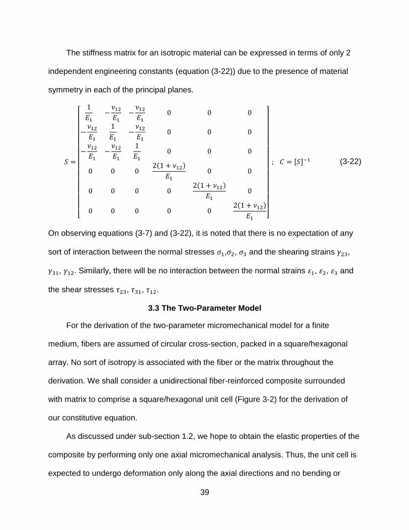
The stiffness matrix for an isotropic material can be expressed in terms of only 2
independent engineering constants (equation (3-22)) due to the presence of material
symmetry in each of the principal planes.
[
( )
( )
( )
]
[ ] (3-22)
On observing equations (3-7) and (3-22), it is noted that there is no expectation of any
sort of interaction between the normal stresses , , and the shearing strains ,
, . Similarly, there will be no interaction between the normal strains , , and
the shear stresses , , .
3.3 The Two-Parameter Model
For the derivation of the two-parameter micromechanical model for a finite
medium, fibers are assumed of circular cross-section, packed in a square/hexagonal
array. No sort of isotropy is associated with the fiber or the matrix throughout the
derivation. We shall consider a unidirectional fiber-reinforced composite surrounded
with matrix to comprise a square/hexagonal unit cell (Figure 3-2) for the derivation of
our constitutive equation.
As discussed under sub-section 1.2, we hope to obtain the elastic properties of the
composite by performing only one axial micromechanical analysis. Thus, the unit cell is
expected to undergo deformation only along the axial directions and no bending or

40
twisting will be involved. This unit cell is assumed to be under a state of uniform
average strain at the macroscopic level called macroscale strains or macrostrains, and
the corresponding axial stresses will be referred to as macrostresses. However, the
microstresses, which are the actual stresses in the constituent phases of the
representative volume element, will have spatial variation. The surface tractions are
assumed to be continuous at the fiber-matrix interface.
b
a
b
a
2
3
1
L1
L2
L3
(A) (B)
Figure 3-2. A unidirectional fiber surrounded by matrix comprising A) square unit cell B) hexagonal unit cell
The effective composite macrostress can be expressed explicitly in terms of the
stress present in the fiber and the matrix phases, and is given by equation (3-2). Using
the constitutive stress-strain relationship, the equation can be rewritten as,

41
(3-23)
∫
∫
Here constitute the unknown microstrains in the fiber or the matrix phases. and ,
respectively represent the fiber- and matrix-phase volumes ( ).
Since there is no macroscale shear deformation,it should be noted that the
respective strain vectors and their corresponding stiffness matrices ( and ) present
in equation (3-23) will be characterized by only the normal stress/strain terms and are
void of any of the shear terms as shown in equations (3-24) and (3-25).
[
]
[ ] (3-24)
(3-25)
The relations presented in equations (3-24) and (3-25) are for the effective
composite stiffness matrix and the effective strain composite strain vectors. Similar
expressions hold true for the corresponding fiber and matrix phases (where effective
elastic properties of the composite are replaced with the corresponding fiber and matrix
properties).
Using equation (3-23), we are able to manipulate the expression and modify it by
adding and subtracting from in the first term. The expression can thus be written
as:
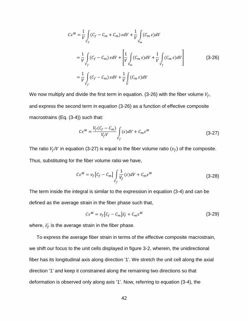
42
∫( )
∫(
)
(3-26)
∫( )
[
∫(
)
∫(
) ]
∫( )
∫(
)
We now multiply and divide the first term in equation. (3-26) with the fiber volume ,
and express the second term in equation (3-26) as a function of effective composite
macrostrains (Eq. (3-4)) such that:
( )
∫(
) (3-27)
The ratio / in equation (3-27) is equal to the fiber volume ratio ( ) of the composite.
Thus, substituting for the fiber volume ratio we have,
[ ] ∫
(
) (3-28)
The term inside the integral is similar to the expression in equation (3-4) and can be
defined as the average strain in the fiber phase such that,
[ ] (3-29)
where, is the average strain in the fiber phase.
To express the average fiber strain in terms of the effective composite macrostrain,
we shift our focus to the unit cells displayed in figure 3-2, wherein, the unidirectional
fiber has its longitudinal axis along direction '1'. We stretch the unit cell along the axial
direction '1' and keep it constrained along the remaining two directions so that
deformation is observed only along axis '1'. Now, referring to equation (3-4), the
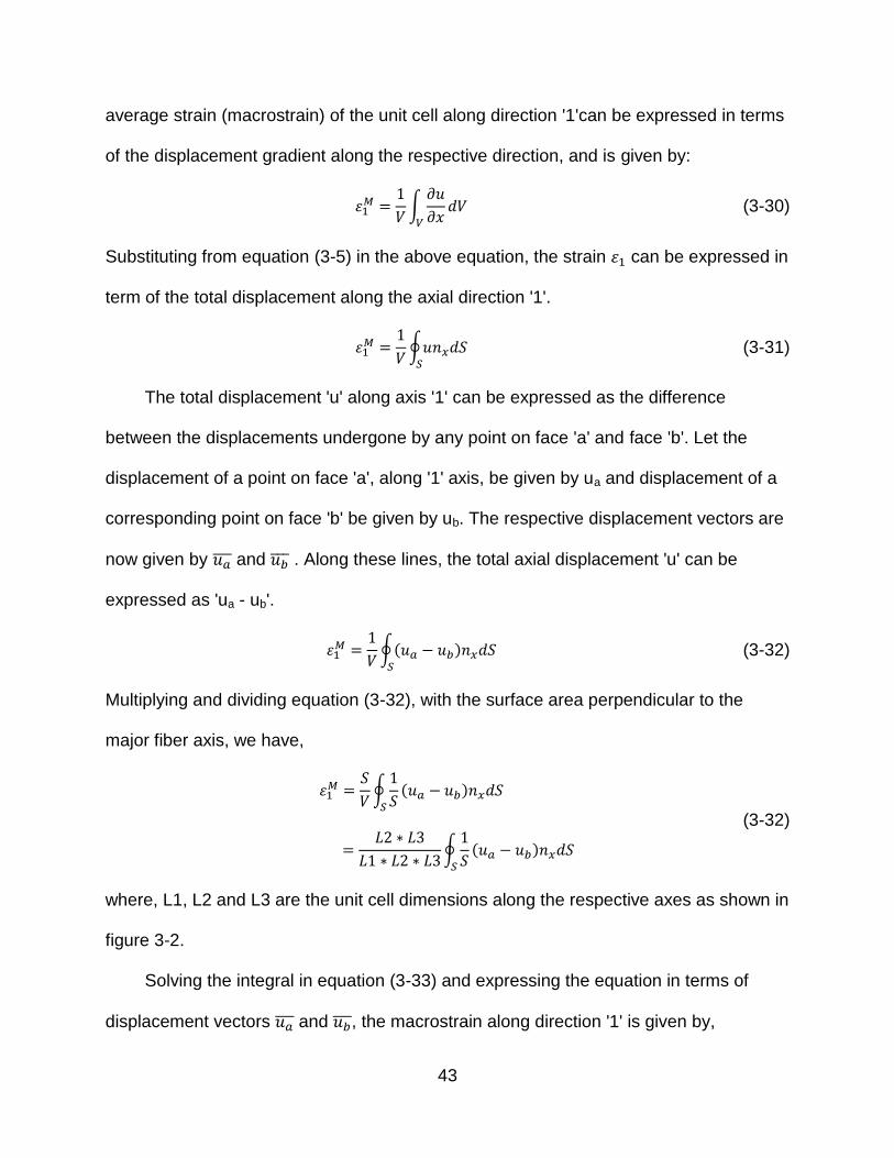
43
average strain (macrostrain) of the unit cell along direction '1'can be expressed in terms
of the displacement gradient along the respective direction, and is given by:
∫
(3-30)
Substituting from equation (3-5) in the above equation, the strain can be expressed in
term of the total displacement along the axial direction '1'.
∮
(3-31)
The total displacement 'u' along axis '1' can be expressed as the difference
between the displacements undergone by any point on face 'a' and face 'b'. Let the
displacement of a point on face 'a', along '1' axis, be given by ua and displacement of a
corresponding point on face 'b' be given by ub. The respective displacement vectors are
now given by and . Along these lines, the total axial displacement 'u' can be
expressed as 'ua - ub'.
∮( )
(3-32)
Multiplying and dividing equation (3-32), with the surface area perpendicular to the
major fiber axis, we have,
∮
( )
∮
( )
(3-32)
where, L1, L2 and L3 are the unit cell dimensions along the respective axes as shown in
figure 3-2.
Solving the integral in equation (3-33) and expressing the equation in terms of
displacement vectors and , the macrostrain along direction '1' is given by,

44
( ) (3-34)
On examining equation (3-34) and figure 3-1, one may note the length L1 of the
unit cell is equal to the fiber length. Also since the front and rear face of the fiber lie on
face 'a' and face 'b' of the unit cell respectively, it can be said that the average strain of
the unit cell is equal to the average fiber strain along '1' axis (the longitudinal axis of the
fiber).
(3-35)
Making use of this property the average fiber strain vector may now be portrayed in
terms of the average composite strain vector such that,
[ ]
(3-36)
where, T is called the volume averaged fiber strain concentration matrix and is defined
as,
[
] [
] (3-37)
Using the relation in equation (3-36) and substituting for in equation (3-29), we
have,
[ ] (3-38)
It is noted that since the macroscopic strain appears in each term of the equation
(3-38), it can be said that the equation holds true for all values of macroscopic strain,
which bring us to a constitutive equation relating the effective composite stiffness matrix
with the constituent fiber and matrix stiffness matrices.
45
[ ] (3-39)
It can thus be concluded, that the effective stiffness matrix (given by equation (3-
24)) of any composite can be obtained using the above equation provided one is able to
calculate each element of the volume averaged fiber strain concentration matrix (i.e. the
T matrix) displayed in Eq. (3-36).
Calculating the T Matrix - Although equation (3-39) holds true for all types of fiber-
reinforced materials, we are only interested in composites with transversely isotropic or
isotropic fiber material. For the calculation of the T matrix, a procedure was developed
keeping in mind the transverse isotropy nature of the fibers. Ergo the elements
constituting the T matrix, for composites with isotropic fibers, are calculated in an
exactly similar fashion. Equation (3-37) has 6 unknown parameters. There are two
phases to calculating these parameters. The former stage which involves finite element
analysis of the RVE (representative volume element), give us four of the six parameters.
The latter stage involves some basic algebra to help deduce the remaining two
parameters.
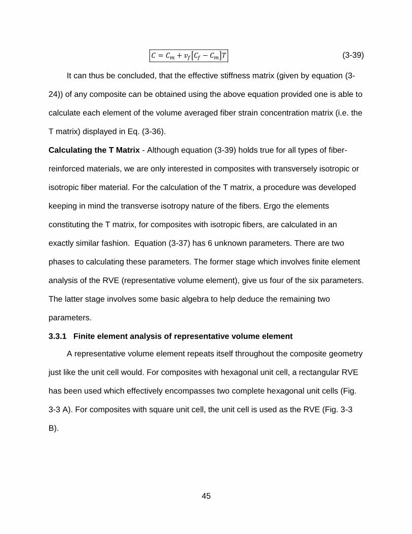
3.3.1 Finite element analysis of representative volume element
A representative volume element repeats itself throughout the composite geometry
just like the unit cell would. For composites with hexagonal unit cell, a rectangular RVE
has been used which effectively encompasses two complete hexagonal unit cells (Fig.
3-3 A). For composites with square unit cell, the unit cell is used as the RVE (Fig. 3-3
B).
46
(A)
(B)
Figure 3-3. Representative volume elements for composites with A) hexagonal unit cells B) square unit cells.
47
The essence of using a rectangualr RVE instead of the hexagonal unit cell lies in the
convinience observed while applying boundary conditions for the finite element analysis
of the cell. With a hexagonal unit cell, we would have to make use of periodic boundary
conditions [37] whereas with the rectangular RVE, the boundary conditions become
very much similar to those for a square unit cell. The boundary conditions are discussed
in detail.
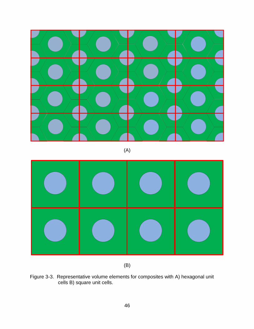
At this point, it would be important to point out that the default axis configuration in
Abaqus is not consistentwith the configuration of a principal material coordinate system.
This anomoly is portrayed in Fig. 3-4.
b
a
2
3
1
b
a
1/x
2/y
3/z
(A) (B)
Figure 3-4. Axis configuration A) used by Abaqus B) a principal material coordinate system.
Although Abaqus displays the coordinate system in terms of x, y and z, we have taken
the liberty to express the same in terms of 1, 2 and 3 for convenience purposes. As a
consequence, utmost care has to be taken while extracting field output values or
48
entering material properties especially for the fiber section, when the fiber properties in
concern are transversely isotropic. Throughout this document, any field variable that
has been obtained from Abaqus, has been portrayed in terms of the coordinate system
used by Abaqus (e.g. S11, E11, etc.). In contrast, all variables associated with the
derivation of the two-paramter model (such as ),and any material constant (e.g. )
have been portrayed using the principal material coordinate system.
A 2D planar deformable part type with base feature shell is chosen for the
micromechanical analysis since we are interested in the behaviour of the RVE cross-
section across the 2-3 plane.The sections are solid homogenous and a plane strain
thickness of 1 unit is assigned to each section of the model.For testing purposes, we
keep the volume fiber ratio fixed at 0.6 (Fig. 3-5). Due to the 1000 node restriction
present in the student version of Abaqus, we are forced to use only quarter of the
representative volume element. It should be noted that using quarter of the RVE does
not affect the axial analysis due to the symmetry of the RVE.This can be confirmed by
performing a full RVE analysis and comparing the results with the analysis of a quarter
of the RVE.
Micromechanical analysis is performed along each of the transverse axes.
Analysis along the 2nd axis will provide us with and . These terms are pretty much
analogous to average strains in the 2nd and 3rd direction respectively, due to the
deformations along 2nd direction. Similarly, micromechanical analysis in the 3rd direction
will provide us with and . The dimensions of the RVE are evidently based on
those for the unit cells. For composites with square unit cells, a square of edge length of
1 unit is used. Similarly, for composites with hexagonal unit cells, a hexagon edge

49
length of 1 unit was used. This resulted in a rectangular RVE of edge length of 1.5 units
along the 2nd direction and edge length of 0.866 units along the 3rd direction.
(A)
(B)
Figure 3-5. 1/4th representative volume element A) for composites with hexagonal unit cells B) for composites with square unit cells. The red sections denote the fiber and the green sections denote the matrix.

50
u = L
L
B
(A)
v = B
L
B
(B)
Figure 3-6. Boundary conditions for RVE analysis A) along direction 2 B) along direction 3.
51
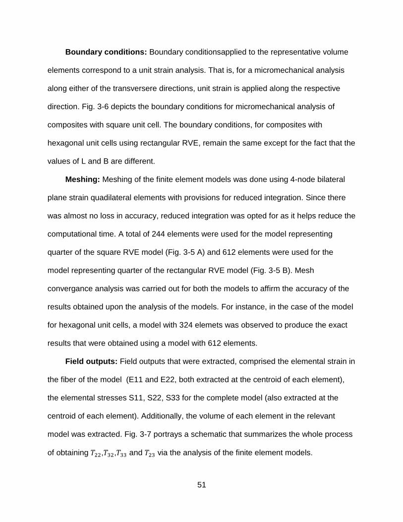
Boundary conditions: Boundary conditionsapplied to the representative volume
elements correspond to a unit strain analysis. That is, for a micromechanical analysis
along either of the transversere directions, unit strain is applied along the respective
direction. Fig. 3-6 depicts the boundary conditions for micromechanical analysis of
composites with square unit cell. The boundary conditions, for composites with
hexagonal unit cells using rectangular RVE, remain the same except for the fact that the
values of L and B are different.
Meshing: Meshing of the finite element models was done using 4-node bilateral
plane strain quadilateral elements with provisions for reduced integration. Since there
was almost no loss in accuracy, reduced integration was opted for as it helps reduce the
computational time. A total of 244 elements were used for the model representing
quarter of the square RVE model (Fig. 3-5 A) and 612 elements were used for the
model representing quarter of the rectangular RVE model (Fig. 3-5 B). Mesh
convergance analysis was carried out for both the models to affirm the accuracy of the
results obtained upon the analysis of the models. For instance, in the case of the model
for hexagonal unit cells, a model with 324 elemets was observed to produce the exact
results that were obtained using a model with 612 elements.
Field outputs: Field outputs that were extracted, comprised the elemental strain in
the fiber of the model (E11 and E22, both extracted at the centroid of each element),
the elemental stresses S11, S22, S33 for the complete model (also extracted at the
centroid of each element). Additionally, the volume of each element in the relevant
model was extracted. Fig. 3-7 portrays a schematic that summarizes the whole process
of obtaining , , and via the analysis of the finite element models.

52
Job analysis for unit strain
Extract E11, E22 at centroid of each
element present in the fiber section of the
model
Multiply the E11 and E22, values with the corresponding
elemental volumes
Extract S11, S22, S33 at the centroid of each
element
Extract the elemental volume for all the
elements
Multiply the S11, S22 and S33 values with the corresponding
elemental volumes
Sum the products and divide the values with the volume of the
fiber section
Sum the products and divide the values with the total volume of
the model
Gives T22 and T32 values when the analysis is carried out along 2nd direction and gives T23 and T33 when the analysis is carried out along
3nd
Gives the 2nd column of the stiffness matrix of the composite
in question when analysis is carried out along 2nd direction
and gives 3rd column of the stiffness matrix when analysis is carried out along 3rd direction
Figure 3-7. Schematic of the procedure followed to obtain , , and .

53
Figure 3-8. displays the deformed hexagonal RVE models with displacement
contours, upon micromechanical analysis along each of composite transverse direction.
(A)
(B)
Figure 3-8. Hexagonal RVE model undergoing unit strain deformation A) along 2nd direction B) along 3rd direction.
54
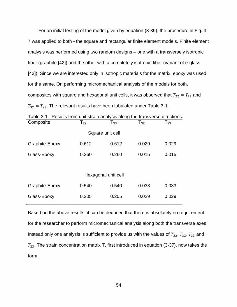
For an initial testing of the model given by equation (3-39), the procedure in Fig. 3-
7 was applied to both - the square and rectangular finite element models. Finite element
analysis was performed using two random designs – one with a transversely isotropic
fiber (graphite [42]) and the other with a completely isotropic fiber (variant of e-glass
[43]). Since we are interested only in isotropic materials for the matrix, epoxy was used
for the same. On performing micromechanical analysis of the models for both,
composites with square and hexagonal unit cells, it was observed that and
. The relevant results have been tabulated under Table 3-1.
Table 3-1. Results from unit strain analysis along the transverse directions.
Composite T22 T33 T32 T23
Square unit cell
Graphite-Epoxy 0.612 0.612 0.029 0.029
Glass-Epoxy 0.260 0.260 0.015 0.015
Hexagonal unit cell
Graphite-Epoxy 0.540 0.540 0.033 0.033
Glass-Epoxy 0.205 0.205 0.029 0.029
Based on the above results, it can be deduced that there is absolutely no requirement
for the researcher to perform micromechanical analysis along both the transverse axes.
Instead only one analysis is sufficient to provide us with the values of , , and
. The strain concentration matrix T, first introduced in equation (3-37), now takes the
form,
55
[
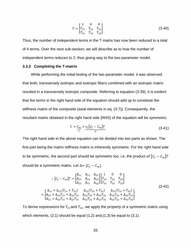
] (3-40)
Thus, the number of independent terms in the T matrix has now been reduced to a total
of 4 terms. Over the next sub-section, we will describe as to how the number of
independent terms reduces to 2, thus giving way to the two-parameter model.
3.3.2 Completing the T-matrix
While performing the initial testing of the two parameter model, it was observed
that both, transversely isotropic and isotropic fibers combined with an isotropic matrix
resulted in a transversely isotropic composite. Referring to equation (3-39), it is evident
that the terms in the right hand side of the equation should add up to constitute the
stiffness matrix of the composite (axial elements in eq. (3-7)). Consequently, the
resultant matrix obtained in the right hand side (RHS) of the equation will be symmetric.
⏟
[ ] ⏟
(3-41)
The right hand side in the above equation can be divided into two parts as shown. The
first part being the matrix stiffness matrix is inherently symmetric. For the right hand side
to be symmetric, the second part should be symmetric too. i.e. the product of [ ]
should be a symmetric matrix. Let [ ].
[ ] [
] [
]
[ ( ) ( ) ( )
]
(3-42)
To derive expressions for and , we apply the property of a symmetric matrix using
which elements, (2,1) should be equal (1,2) and,(1,3) be equal to (3,1).

56
( )
( ) (3-43)
Equation (3-43) presents a simultaneous set of linear equations. To solve the set of
equations, we multiply the first equation with , and the second equation with ,
which brings us to,
( )
( )
(3-44)
Subtracting the second equation from the first, we get,
( )
(3-44)
The symmetry in a composite with transversely isotropic stiffness matrix thus leads us
to,
( )
(3-45)
Hence, making use of equations (3-40) and (3-45), it is concluded that the T matrix can
be computed by performing single micromechanical analysis along any of the material
transverse directions. That is, each element in the T matrix can be expressed in terms
of two parameters - either and , or and . In other words, knowledge of
these two parameters along with the material properties of the constituent materials is
sufficient enough for the calculation of the stiffness matrix , hence the name of the
model.

57
CHAPTER 4 RESPONSE SURFACE PREDICTION OF THE PARAMETERS – T22 AND T32
4.1 Surrogate Modeling Using Polynomial Response Surfaces
A response surface methodology portrays the relationship between several
explanatory (independent) variables and one or more response (dependent) variables.
The method was first introduced by G. E. P. Box and K. B. Wilson in 1951 [35]. The
essential thought behind developing the response surface methodology was to use a
sequence of controlled designed experiments to obtain an optimal response. It is
important to acknowledge that this model is only an approximation, but is widely used
because such a model is easy to estimate and apply, even when little is known about
the process. In the ensuing paragraphs, basic terminologies and error measures
involved in fitting an approximation to a set of data have been discussed.
In its most generic form, a response function y (that needs to be approximated),
can be denoted as a combination of (approximated function of a design variable
vector x and a vector of parameters ), and is the vector of errors associated with
the curve fit.
( ) (4-1)
One has the data obtained from experiments at design points. If each design
point is denoted by , then,
( ) (4-2)
Our main objective is to find the set of parameters , that will best fit the experimental
data. The process of finding the vector which best fits the experimental data, is called
regression and is called a response surface.
58
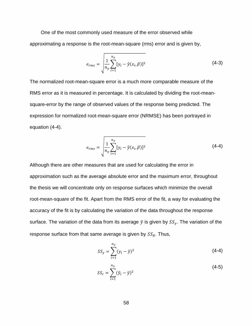
One of the most commonly used measure of the error observed while
approximating a response is the root-mean-square (rms) error and is given by,
√
∑[ ( )]
(4-3)
The normalized root-mean-square error is a much more comparable measure of the
RMS error as it is measured in percentage. It is calculated by dividing the root-mean-
square-error by the range of observed values of the response being predicted. The
expression for normalized root-mean-square error (NRMSE) has been portrayed in
equation (4-4).
√
∑[ ( )]
(4-4)
Although there are other measures that are used for calculating the error in
approximation such as the average absolute error and the maximum error, throughout
the thesis we will concentrate only on response surfaces which minimize the overall
root-mean-square of the fit. Apart from the RMS error of the fit, a way for evaluating the
accuracy of the fit is by calculating the variation of the data throughout the response
surface. The variation of the data from its average is given by . The variation of the
response surface from that same average is given by . Thus,
∑( )
(4-4)
∑( )
(4-5)

59
The ratio of to denoted by , measures the fraction of the variation in data as
captured by the response surface. As explained in [38], increasing the number of
coefficients increases the value of . This by no means conveys the statement that the
prediction capabilities of the response surface have improved. And hence, there is an
adjusted form of as depicted in [38], which is given by equation (4-6).
( ) (
) (4-6)
Thus, the adjusted value of is a better measure of goodness of fit. It is important to
note that if this value decreases upon increasing the number of coefficients, it is a sign
that we might be fitting the data better but losing out on the predictive capabilities of the
response surface.
A much more reliable measure of the predictive capabilities of the response
surface is testing it at the data points which have not been used in its construction.
Instead of carrying out additional tests or numerical evaluations, the predictive capability
can be checked by leaving out a few points will not change drastically the quality of the
fit. This can only be done provided the number of points used for the fit is substantially
larger than the number of coefficients. We can thus leave out a few points, fit the
response surface to the remaining points and then check the error at the points that
have been left out. The idea is to continue this procedure with other points till each point
has been left out once. This procedure is commonly known as cross validation. Ideally,
cross validation is usually done leaving one point at a time. Since we are using the sum
of the squares of the prediction errors as a measure of the predictive accuracy of the
response surface, the error is termed as PRESS RMS error (for prediction error sum of
squares). We will make use of the normalized PRESS RMS error (N-PRESS RMSE,

60
calculated in a fashion similar to that of NRMSE) which expresses the PRESS RMS
error in percentage. As mentioned in section 1.2, the program for constructing a
polynomial response surface has been extracted from a surrogate toolbox created by
Felipe A.C.Viana [2].
Design of Experiments (DOEs) - Selecting the points in the design space where
experiments are to be performed is probably the most important part of obtaining good
approximations to any response system. These points where experiments are to be
performed are known as design of experiments. Design of experiments is inherently a
multi-objective optimization problem. Points should be selected so as maximize the
accuracy of the information gathered from the experiments. At the same time, it is
advisable to achieve this accuracy through a minimum number of experiments to help
reduce the overall optimization cost. Hence, it can be said that our primary goal while
choosing the design of experiments, is to choose points that will maximize the predictive
capability of the model. There are various ways of generating a certain set of design of
experiments such as the 2-level full factorial design, central composite design and LHS
deign.
For creating our DOEs, a design space was generated using the Latin Hypercube
Sampling function provided in MATLAB. The technique was first presented by McKay in
1979 [39]. Latin hypercube sampling (LHS) is a statistical method for generating a
distribution of plausible collections of parameter values from a multidimensional
distribution [41]. The sampling method is often applied in uncertainty analysis. In LHS,
for a set of ‘n’ points, each variable range is divided into ‘n’ equal probability intervals
with one point at each interval. A big advantage of using LHS design space is that the
61
design points are better distributed for each variable as depicted in Figure 5.6. A
downfall of the method is that even though the design points are well spread out, there
are still some voids left in between the data points. To overcome this problem, we
perform multiple iterations in an attempt to maximize the minimum distance between
points. This helps to populate the entire design space. A more comprehensive study on
the topic of response surface methodology has been presents in [30-31, 38, 40].
It is important to note that the LHS function in MATLAB produces DOEs in a range
of zero to one. They have to be scaled to the respective variable ranges in order to
render them usable.
4.2 Constructing the Response Surface
The knowledge of and is sufficient enough for the prediction of the stiffness
matrix of the composite given by equation (3-24) and thus, the prediction of materials
constants , , , .As noted previously, transversely isotropic fibers and isotropic
fibers, both individually combined with an isotropic matrix, result in a transversely
isotropic composite. Hence, the only material constant that is not obtained using the
two-parameter model is , for which, a separate response surface is devloped
(chapter 5). As discussed in section 1.2, the response surfaces have been constructed
only for circular fibers in a hexagonal array.
4.2.1 Selection of Variables And Generation of Design Points
Since we are interested in only isotropic materials forming the matrix, from
equation (3-39) it is evident that the parameters depend on the,
Longitudinal Young’s modulus - , , belonging to the fiber and the matrix
respectively.
62
Transverse Young’s modulus - , , belonging to the fiber and the matrix
respectively.
Longitudinal Poisson’s ratio - , belonging to the fiber and the matrix
respectively.
Transverse Poisson’s ratio - , belonging to the fiber and the matrix
respectively.
Fiber volume fraction, .
The range of the material constants (those listed above along with the longitudinal shear
modulus) for both, the fiber and the matrix was chosen based on the data encountered
across various sources of literature, such that,
(4-7)
Equation (4-7) presents the range of material constants for composites with transversely
isotropic fibers. For composites using completely isotropic fibers, the ranges that were
taken into account were those of ⁄ and, . It should be
noted that although the two-parameter model does not require the knowledge of the
value of longitudinal shear modulus for either of the fiber or matrix, Abaqus as an
analysis software needs the complete information for each material used in the model.

63
Points were generated based on the variables listed in equation (4-7). For the
selection of the design of experiments, ‘lhsdesign’ function in MATLAB was used with a
criterion for minimizing the minimum distance between any two points in the design
space. 100 designs were generated for composites with transversely isotropic fiber and
40 designs for composites with isotropic fiber. In an effort to make the numerical ranges
across all the variables uniform, and make the variable data points more generic, 5
variables were chosen such that the final set of variables used in constructing the
response surface is given by,
(
) (
)
(4-8)
The design points generated using the variables in equation (4-7) were propagated to
the set of variables in equation (4-8). This generic set of variables allowed for the
possible selection of a consistent isotropic design to be used for the matrix, throughout
each of the 140 simulations. The isotropic design was accorded material values of
and .
4.2.2 Constructing and Choosing an Accurate Response Surface
Simulations were carried out at each of the orthotropic and isotropic design points.
For each simulation a set of parameters and was obtained (i.e. 140 sets of
parameters were recorded). Thus, independent response surfaces were constructed for
the prediction of and (i.e. at a time, a response surface can predict only one of
the two parameters). An initial predictive capability test involving various types and
degrees of polynomial response surfaces was carried out, for six real world composite
designs to check the average error in prediction of each fit. The volume fiber ratio was
maintained at a constant value of 60% for each of the six composite designs and, epoxy
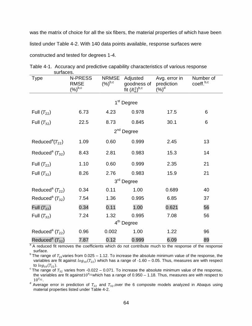
64
was the matrix of choice for all the six fibers, the material properties of which have been
listed under Table 4-2. With 140 data points available, response surfaces were
constructed and tested for degrees 1-4.
Table 4-1. Accuracy and predictive capability characteristics of various response surfaces.
Type N-PRESS RMSE (%)b,c
NRMSE (%)b,c
Adjusted goodness of
fit ( )b,c
Avg. error in prediction (%)d
Number of coeff.b,c
1st Degree
Full ( ) 6.73 4.23 0.978 17.5 6
Full ( ) 22.5 8.73 0.845 30.1 6
2nd Degree
Reduceda( ) 1.09 0.60 0.999 2.45 13
Reduceda ( ) 8.43 2.81 0.983 15.3 14
Full ( ) 1.10 0.60 0.999 2.35 21
Full ( ) 8.26 2.76 0.983 15.9 21
3rd Degree
Reduceda ( ) 0.34 0.11 1.00 0.689 40
Reduceda ( ) 7.54 1.36 0.995 6.85 37
Full ( ) 0.34 0.11 1.00 0.621 56
Full ( ) 7.24 1.32 0.995 7.08 56
4th Degree
Reduceda ( ) 0.96 0.002 1.00 1.22 96
Reduceda ( ) 7.87 0.12 0.999 6.09 89 a
A reduced fit removes the coefficients which do not contribute much to the response of the response surface.
b The range of varies from 0.025 – 1.12. To increase the absolute minimum value of the response, the
variables are fit against ( ) which has a range of -1.60 – 0.05. Thus, measures are with respect to ( ).
c The range of varies from -0.022 – 0.071. To increase the absolute minimum value of the response,
the variables are fit against which has a range of 0.950 – 1.18. Thus, measures are with respect to
. d
Average error in prediction of and ,over the 6 composite models analyzed in Abaqus using material properties listed under Table 4-2.
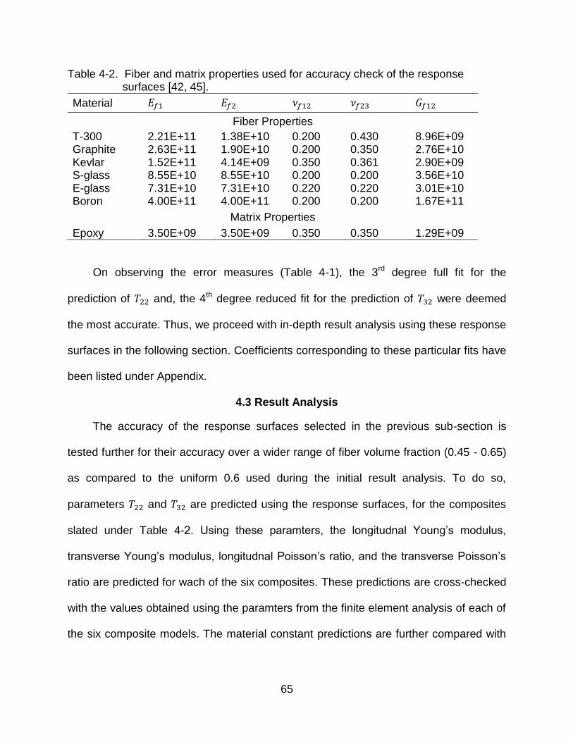
65
Table 4-2. Fiber and matrix properties used for accuracy check of the response surfaces [42, 45].
Material
Fiber Properties
T-300 2.21E+11 1.38E+10 0.200 0.430 8.96E+09 Graphite 2.63E+11 1.90E+10 0.200 0.350 2.76E+10 Kevlar 1.52E+11 4.14E+09 0.350 0.361 2.90E+09 S-glass 8.55E+10 8.55E+10 0.200 0.200 3.56E+10 E-glass 7.31E+10 7.31E+10 0.220 0.220 3.01E+10 Boron 4.00E+11 4.00E+11 0.200 0.200 1.67E+11
Matrix Properties
Epoxy 3.50E+09 3.50E+09 0.350 0.350 1.29E+09
On observing the error measures (Table 4-1), the 3rd degree full fit for the
prediction of and, the 4th degree reduced fit for the prediction of were deemed
the most accurate. Thus, we proceed with in-depth result analysis using these response
surfaces in the following section. Coefficients corresponding to these particular fits have
been listed under Appendix.
4.3 Result Analysis
The accuracy of the response surfaces selected in the previous sub-section is
tested further for their accuracy over a wider range of fiber volume fraction (0.45 - 0.65)
as compared to the uniform 0.6 used during the initial result analysis. To do so,
parameters and are predicted using the response surfaces, for the composites
slated under Table 4-2. Using these paramters, the longitudnal Young’s modulus,
transverse Young’s modulus, longitudnal Poisson’s ratio, and the transverse Poisson’s
ratio are predicted for wach of the six composites. These predictions are cross-checked
with the values obtained using the paramters from the finite element analysis of each of
the six composite models. The material constant predictions are further compared with

66
the results obtained using the Halpin-Tsai (HT) equations ( Eqs. (2-6 – 2-7) for and
) and the rule of mixtures ( Eq. (2-1) for and ).
4.3.1 Adopting a Reliable Estimate for the Halpin-Tsai Parameter,
It is critical to determine a value of the parameter to be used in the Halpin-Tsai
model (Eq. (2-6)). Although the use of for calculating the transverse elastic
modulus is consensus in the world of composites using circular fibers in a square array,
this value doesn’t work well for circular fibers in a hexagonal array. In fact, for circular
fibers in a hexagonal array, we don’t have an explicit value for the parameter [37].
To find a reliable estimate of , the data was extracted from all the FE based
simulations such that there were 140 values available for both and .Using
backward calculations (proceeding with known values of , and arriving at a value
for ), an value of 0.73 was found to give good results when predicting ( is
obtained using Eq. (3-8)) of composites with transversely isotropic fibers. However, this
iterative method did not work well for composites having completely isotropic fibers.
Instead, it was observed that the value increased with an increase in the value of the
volume fiber fraction (Fig. 4-1A). An approximate solution to this problem is given by
fitting a curve between and the volume fiber fraction using data points
corresponding to composites with only isotropic fibers, such that,
(4-9)
A similar problem was encountered in the process of obtaining a reasonable estimate of
for the calculation of (Fig. 4-1B). The expression obtained by fitting a curve
between and the volume fiber fraction in this case is given by,
(4-10)
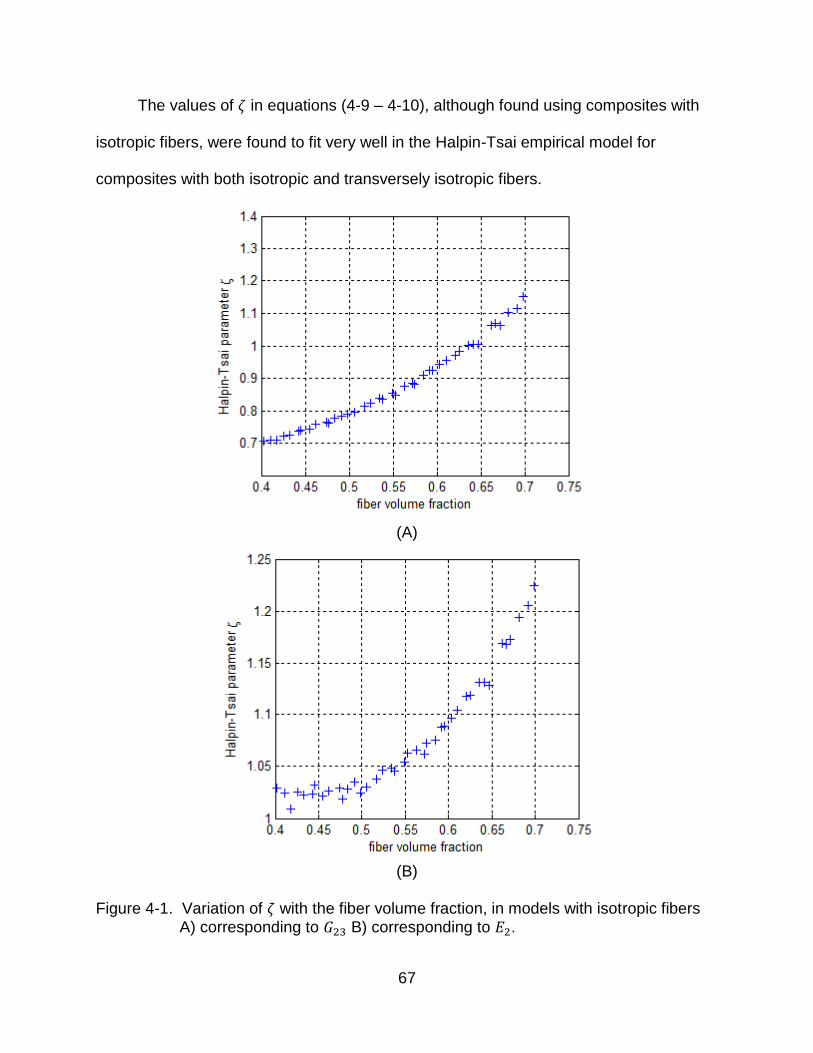
67
The values of in equations (4-9 – 4-10), although found using composites with
isotropic fibers, were found to fit very well in the Halpin-Tsai empirical model for
composites with both isotropic and transversely isotropic fibers.
(A)
(B)
Figure 4-1. Variation of with the fiber volume fraction, in models with isotropic fibers A) corresponding to B) corresponding to .
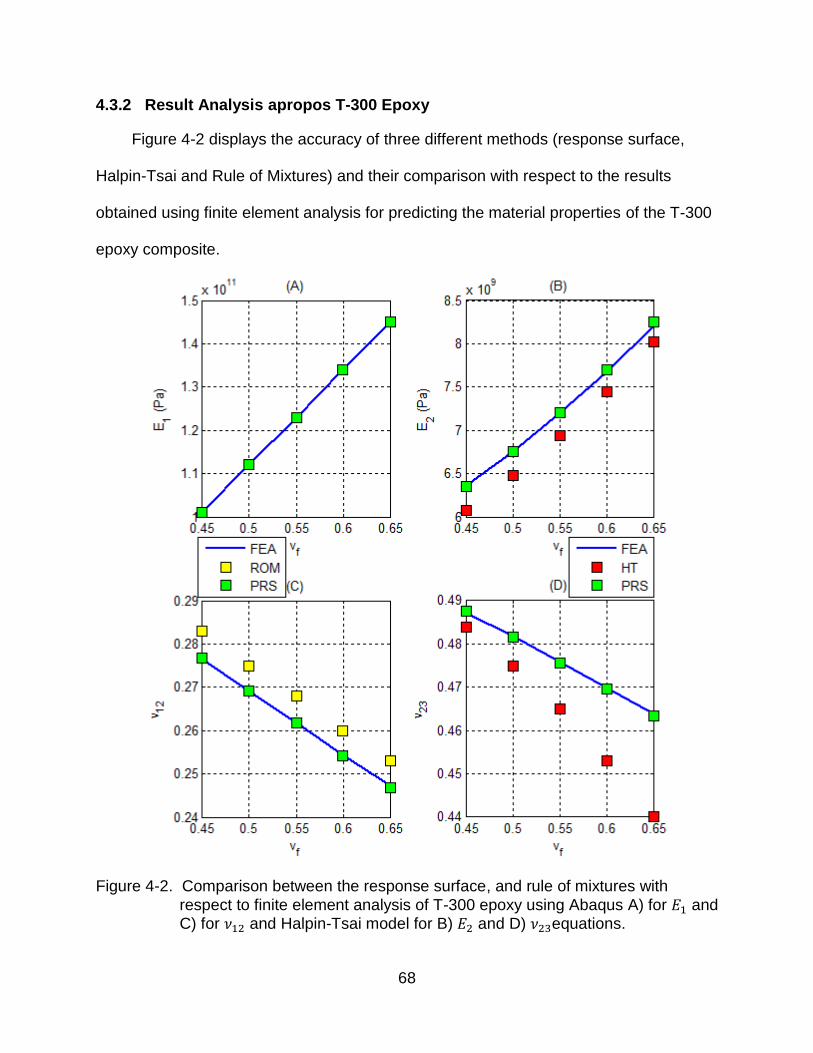
68
4.3.2 Result Analysis apropos T-300 Epoxy
Figure 4-2 displays the accuracy of three different methods (response surface,
Halpin-Tsai and Rule of Mixtures) and their comparison with respect to the results
obtained using finite element analysis for predicting the material properties of the T-300
epoxy composite.
Figure 4-2. Comparison between the response surface, and rule of mixtures with
respect to finite element analysis of T-300 epoxy using Abaqus A) for and C) for and Halpin-Tsai model for B) and D) equations.
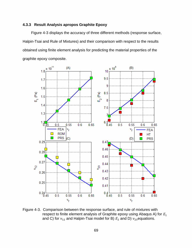
69
4.3.3 Result Analysis apropos Graphite Epoxy
Figure 4-3 displays the accuracy of three different methods (response surface,
Halpin-Tsai and Rule of Mixtures) and their comparison with respect to the results
obtained using finite element analysis for predicting the material properties of the
graphite epoxy composite.
Figure 4-3. Comparison between the response surface, and rule of mixtures with
respect to finite element analysis of Graphite epoxy using Abaqus A) for and C) for and Halpin-Tsai model for B) and D) equations.

70
4.3.4 Result Analysis apropos Kevlar Epoxy
Figure 4-4 displays the accuracy of three different methods (response surface,
Halpin-Tsai and Rule of Mixtures) and their comparison with respect to the results
obtained using finite element analysis for predicting the material properties of the Kevlar
epoxy composite.
Figure 4-4. Comparison between the response surface, and rule of mixtures with
respect to finite element analysis of Kevlar epoxy using Abaqus A) for and C) for and Halpin-Tsai model for B) and D) equations.

71
4.3.5 Result Analysis apropos S-glass Epoxy
Figure 4-5 displays the accuracy of three different methods (response surface,
Halpin-Tsai and Rule of Mixtures) and their comparison with respect to the results
obtained using finite element analysis for predicting the material properties of the S-
glass epoxy composite.
Figure 4-5. Comparison between the response surface, and rule of mixtures with
respect to finite element analysis of S-glass epoxy using Abaqus A) for and C) for and Halpin-Tsai model for B) and D) equations.

72
4.3.6 Result Analysis apropos E-glass Epoxy
Figure 4-6 displays the accuracy of three different methods (response surface,
Halpin-Tsai and Rule of Mixtures) and their comparison with respect to the results
obtained using finite element analysis for predicting the material properties of the E-
glass epoxy composite.
Figure 4-6. Comparison between the response surface, and rule of mixtures with
respect to finite element analysis of E-glass epoxy using Abaqus A) for and C) for and Halpin-Tsai model for B) and D) equations.
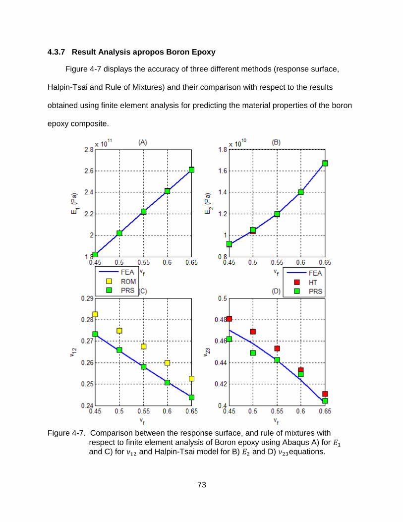
73
4.3.7 Result Analysis apropos Boron Epoxy
Figure 4-7 displays the accuracy of three different methods (response surface,
Halpin-Tsai and Rule of Mixtures) and their comparison with respect to the results
obtained using finite element analysis for predicting the material properties of the boron
epoxy composite.
Figure 4-7. Comparison between the response surface, and rule of mixtures with
respect to finite element analysis of Boron epoxy using Abaqus A) for and C) for and Halpin-Tsai model for B) and D) equations.

74
CHAPTER 5 PREDICTING THE LONGITUDNAL SHEAR MODULUS
The stiffness matrix of a transversely isotropic composite has 5 independent
material constants (Eq. (3-7)). In the previous chapter, we focused on the two
parameter models combined with response surfaces for accurate prediction of 4
( , , , ) of these constants. For the fifth constant, the longitudinal shear modulus
, a distinct method resulting in a separate response surface, is adopted. This method
has been tested only for composites with a hexagonal array of unit cells.
5.1 Extracting Using Abaqus
Due to the inconsistency portrayed by the Abaqus coordinate system (Fig. 3-4), it
is not possible to calculate directly as a field output. As a result, we will be using
Abaqus to calculate (which corresponds to in the material coordinate system).
There are two phases that lead to the calculation of . The first is the finite element
analysis of the hexagonal RVE model to obtain the displacement along the z direction
(w). The second phase consists of a MATLAB program to calculate using the
displacement, w.
5.1.1 Analysis of the Hexagonal Finite Element Model
Although exactly similar in terms of design, to the hexagonal RVE model (Fig. 3-5
B) is used for the finite element analysis, this model is constructed in a 3D design space
in contrast to the earlier use of a 2D design space. This allows for deformation along the
z axis. Homogenous shell type sections are used throughout the model. For the mesh,
4-node shell elements have been used. This type of element helps avoid shear locking.
The essence of using shell elements lies in the fact that they can be curved and they
carry bending stresses.
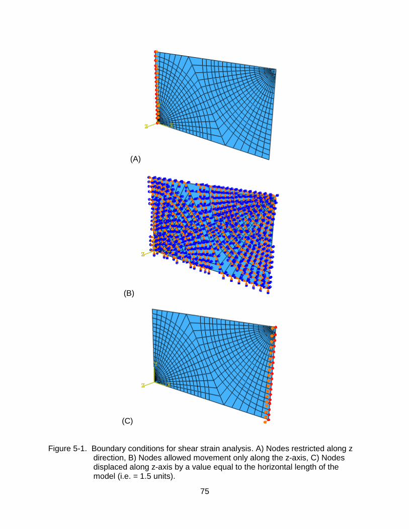
75
(A)
(B)
(C)
Figure 5-1. Boundary conditions for shear strain analysis. A) Nodes restricted along z direction, B) Nodes allowed movement only along the z-axis, C) Nodes displaced along z-axis by a value equal to the horizontal length of the model (i.e. = 1.5 units).

76
Boundary Conditions: The boundary conditions have been applied such that the
model is under an average shear strain of unity, in the x-z plane. The complete set of
boundary conditions adopted, have been depicted in Figure 5-1.It should be pointed out,
that in Figure 5-1(B), the set of nodes in question do not include any of the nodes along
the right or left edges of the model.
Field outputs: Field outputs that were extracted, comprised only of the nodal
displacement, w. Fig. 5-2 shows the displacement countours of the finite element model
under a state of unit shear strain in x-z plane.
Figure 5-2. Hexagonal RVE model undergoing unit shear strain deformation in the x-z plane.
5.1.2 Using Displacement along Z-axis to Calculate
In this section, we make use of physical to reference element mapping to achieve
the desired result. Each element in the finite element model, also referred to as the
physical element, can be mapped to a four-node iso-parametric quadrilateral element
(Fig. 5-3) also referred to as the reference element.

77
t
s
1 (-1,-1)
2 (1,-1)
3 (1,1,)
4 (-1,1,) (1-t)=0
(1-s)=0
(1+t)=0
(1+s
)=0
1
2(w2)
3 (w3)
4(w4)
(w1)
y
x
Figure 5-3. Four-node quadrilateral reference element defined using an s-t coordinate
system.
Numerical value of any physical variable (such as displacement, force, etc.) for
each physical element is approximated using numerical integration. This involves
calculating the variable at each integration point (marked as a cross in the reference
element) and adding them up. Our parametric element is a case of 2-point integration in
a 2D space, the numerical integration of which is given by [1],
∫ ∫ ( )
∑ ∑
( )
(5-1)
Where, for a 2-point integration system. For calculating , the physical
variable, in our case is ⁄ (explained later in the section).
The displacement (w) and coordinate (x, y) of any point in the physical element, in
terms of the parametric coordinate system are given by,
(5-2)

78
Here, are shape functions corresponding to each node of the reference
element, and are given by,
( )( )
(5-3) ( )( )
( )( )
( )( )
The values corresponding to and at each of the four integration points in the
reference element are given by,
( )
√
( )
√
(5-4)
Using chain rule of differentiation in equation (5-3), it can be said that,
(5-5)
Expressing in matrix form,
⏟
[
⁄
⁄
⁄
⁄
]
⏟
⏟
(5-6)
[ ]
Here is the Jacobian matrix and it plays an important role in evaluating the validity of
the mapping as well as the quadrilateral element [44]. The expression in equation (5-6)
is a function of and and should be multiplied with the determinant of the Jacobian

79
matrix to account for the disparity in volume of the element, in real and parametric
space. Thus,
( ) [ ] (5-7)
To obtain ⁄ for an element, the matrix in the above equation should be
calculated at every integration point for the particular element (Eq. (5-1)).
Recalling the expression for shear strain from elasticity theory, we have,
(5-8)
Due to restrained movement allowed along x and y axes, ⁄ .Thus, with the
knowledge of ⁄ for each element, equation (5-8) is used to calculate for each
element (depending on the section in which the element falls, each element will have
value belonging to the fiber or the matrix material). Summing the value for all
elements, and dividing by the volume of the complete model, we obtain the value for
the given composite (note that an average shear strain of 1 was applied).
When implementing calculations in MATLAB, triangular elements in the physical
model are interpreted in terms of an equivalent physical quadrilateral element [1] .
1
2
3 3
y
x
21
3
Figure 5-4. Quadrilateral equivalent of a triangular reference element.
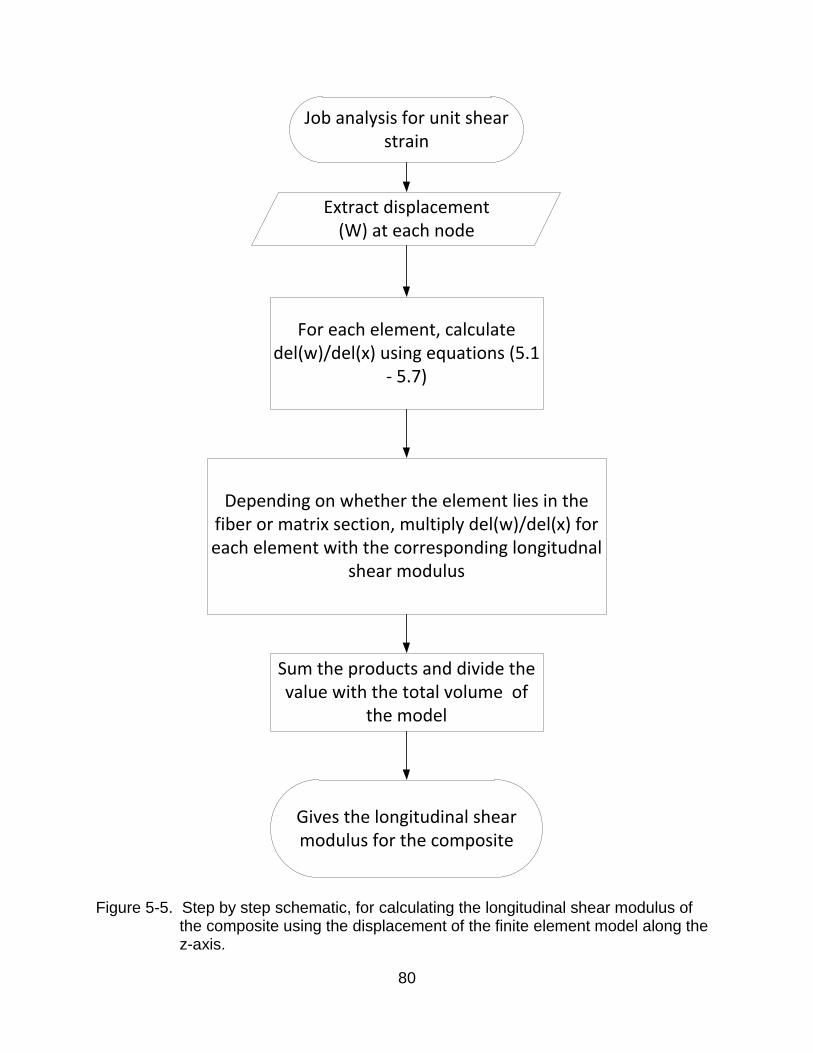
80
Job analysis for unit shear strain
Extract displacement (W) at each node
For each element, calculate del(w)/del(x) using equations (5.1
- 5.7)
Depending on whether the element lies in the fiber or matrix section, multiply del(w)/del(x) for each element with the corresponding longitudnal
shear modulus
Sum the products and divide the value with the total volume of
the model
Gives the longitudinal shear modulus for the composite
Figure 5-5. Step by step schematic, for calculating the longitudinal shear modulus of
the composite using the displacement of the finite element model along the z-axis.

81
5.2 Predicting Using Polynomial Response Surface
The unit shear strain analysis was performed for each of the 100 transversely-
isotropic designs generated for the two-parameter model. Wholly isotropic design were
not used due to the variables (Eq. 5-9) being independent of the directionality of the
composite models.
(
) (5-9)
Figure 5-6 depicts the distribution of the fiber longitudinal shear modulus with respect to
the volume fiber ratio for the 100 transversely-isotropic composite designs generated
using Latin hypercube sampling (LHS). As there were six variables used during the
design point generations, the designs do not appear to be as evenly generated as they
would with all the variables in a six dimensional space (Eq. 4-7).
Figure 5-6. Variation of fiber longitudinal shear modulus with respect to the volume
fiber ratio .
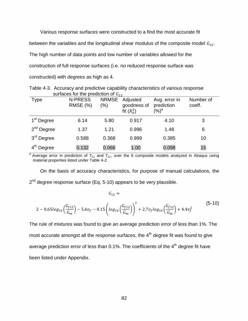
82
Various response surfaces were constructed to a find the most accurate fit
between the variables and the longitudinal shear modulus of the composite model .
The high number of data points and low number of variables allowed for the
construction of full response surfaces (i.e. no reduced response surface was
constructed) with degrees as high as 4.
Table 4-3. Accuracy and predictive capability characteristics of various response
surfaces for the prediction of
Type N-PRESS RMSE (%)
NRMSE (%)
Adjusted goodness of
fit ( )
Avg. error in prediction (%)a
Number of coeff.
1st Degree 6.14 5.80 0.917 4.10 3
2nd Degree 1.37 1.21 0.996 1.48 6
3rd Degree 0.588 0.368 0.999 0.385 10
4th Degree 0.132 0.066 1.00 0.098 15 a
Average error in prediction of and , over the 6 composite models analyzed in Abaqus using material properties listed under Table 4-2.
On the basis of accuracy characteristics, for purpose of manual calculations, the
2nd degree response surface (Eq. 5-10) appears to be very plausible.
(5-10)
(
) ( (
))
(
)
The rule of mixtures was found to give an average prediction error of less than 1%. The
most accurate amongst all the response surfaces, the 4th degree fit was found to give
average prediction error of less than 0.1%. The coefficients of the 4th degree fit have
been listed under Appendix.

83
CHAPTER 6 CONCLUSION
6.1 Summary
We studied the history of micromechanics dating more than a century back. One of
the most important theories in micromechanics, being that of Eshelby’s which set the
trend for modern day micromechanics. It is shown, that for a transversely isotropic
composite using a hexagonal array of cells, the transverse shear modulus, is a
function of the transverse Poisson’s ratio , and the transverse Young’s modulus .
A micromechanical model, was derived based on Eshelby’ theory for
inhomogeneous material, for the prediction of , , , of a transversely isotropic
composite, the accuracy of which was confirmed for composites using either a square
or a hexagonal array of cells. Using finite element based analysis, it was proved that
unit strain analysis along any one of the material transverse directions is sufficient
enough for the two-parameter model to function accurately.
Surrogate modeling of the two parameters (for composites using a hexagonal
array of cells only) using polynomial response surfaces was carried out for the accurate
prediction of the elastic constants , , , . The response surfaces were
constructed based on the data obtained from 140 individua simulations of composite
designs generated using Latin hypercube sampling. The designs were generated
keeping in mind a certain range of design variables.
An effort was made to come up with an accurate expression for the Halpin-Tsai
parameter . In case of composites with completely isotropic fiber, there was a
quadratic trend observed between the parameter and the volume fiber fraction, based
on which, a second degree response surface was constructed. The expression

84
obtained, was found to be fairly accurate, when tested for composties with transversely
isotropic fibers.
In-depth result analysis of six real world composite designs was carried out
wherein the elastic constants obtained using the two-paramter model, the Halpin-Tsai
model and the rule of mixtures, were compared against the results obtained finte
element analysis. The rule of mixtures, as expected gave highly accurate results for .
However, the results were not so convincing for the prediction of using the rule of
mixtures. The Halpin-Tsai model was found to give highly accurate results for the
prediction of , in the case for composites with isotropic fibers, but there was a fair
amount of error when composites with transversely isotropic fiber were taken into
account. This discrepancy was primarily due to the Halpin-Tsai parameter being based
solely on composites with completely isotropic fiber. For the two-paramter model, the
prediction error was very low for all four of the elastic constants except for a few
instances wherin the value of certain curve fit variables might have exceeded the range
based on which the response surfaces were fitted in the first place.
A separate response surface, based on shear strain simluations of finite element
models in 3D space, was constructed for the prediction of . Due to the inconsistency
in Abaqus and material coordinate system, the displacement along the z-axes was used
to arrive at using methods of numerical integration. The accuracy of this response
surface was tested using the six real world composite designs. Although prediction
using a 2nd degree fit were deemed accurate enough, a further 4th degree fit was found
to give results more accurate that the rule of mixtures for (which was found to give
average prediction error of less than 1%).

85
6.2 Future Scope of Work
Although a fairly accurate response surface has been provided for the prediction of
the elastic constants , , , , the trend for the prediction of the parameter was
found to be highly erratic. A solution to this problem might be to try various options in
the field of surrogate modeling that might help in a more accurate and consistent
prediction of . Another issue with the current response surface is that it may not cater
well to the needs of those interested in composites having variable values falling outside
the range specified.
Another area of concern was the Halpin-Tsai parameter which was derived solely
on the basis of the data relating that of the composites using only isotropic fibers. And
even though, the parameter was found to be agreeable for composites withtransversely
isotropic fibers, the results were not as accurate for the same. Hence, a problem may
be posed where in one might find the optimal value of the paramter .
The proceedings of the research will be put in to setting up a website or a program
that will have the response surface data including the coefficient values pre-fed so as to
give the user the values of the elastic constant with respect to the design variable
he/she may enter.

86
APPENDIX RESPONSE SURFACE COEFFICENTS
A.1 For The Prediction Of And
Table A-1.Variable interpretation of numbers
Number Variable Interpretation
1 ( ⁄ )
2 ( ⁄ )
3 ( )⁄
4 ( ⁄ )
5
Table A-2.Coefficients corresponding to the 3rd degree full response surface for
Variable Coefficient Variable Coefficient
'0'a -0.2446 '1.2.4' 0.0080 '1' 0.3373 '1.2.5' -0.0161 '2' -0.6991 '1.3.3' 0.1458 '3' 1.3014 '1.3.4' 0.1555 '4' -1.0992 '1.3.5' 0.1637 '5' 1.0437 '1.4.4' -0.1501 '1.1' -0.1916 '1.4.5' -0.2382 '1.2' 0.0384 '1.5.5' -0.0026 '1.3' -0.6110 '2.2.2' 0.0301 '1.4' 0.4968 '2.2.3' -0.1353 '1.5' -0.0298 '2.2.4' -0.0555 '2.2' -0.1216 '2.2.5' -0.2281 '2.3' -0.3600 '2.3.3' 0.0143 '2.4' 0.4207 '2.3.4' 0.0700 '2.5' -0.1160 '2.3.5' 0.0777 '3.3' -0.5120 '2.4.4' -0.2551 '3.4' -0.6964 '2.4.5' 0.2562 '3.5' 0.6904 '2.5.5' 0.8349 '4.4' 0.8543 '3.3.3' -0.0220 '4.5' -0.7302 '3.3.4' 0.3315 '5.5' -1.4123 '3.3.5' -0.1803 '1.1.1' 0.0495 '3.4.4' 0.1039 '1.1.2' -0.0699 '3.4.5' -0.7498 '1.1.3' -0.0043 '3.5.5' 0.0790 '1.1.4' -0.0470 '4.4.4' -0.2857 '1.1.5' 0.0313 '4.4.5' 0.8290 '1.2.2' 0.0568 '4.5.5' -0.1743 '1.2.3' 0.2119 '5.5.5' 0.7691
a ‘0’ denotes a constant

87
Table A-3.Coefficients corresponding to the 4th degree reduced response surface for
Variable Coefficient Variable Coefficient Variable Coefficient
'2' 0.8316 '1.1.3.3' 1.4626 '3.3.3.5' -1.7475 '3' 4.1193 '1.1.3.4' -1.7163 '3.3.5.5' -3.3953 '4' 1.1897 '1.1.3.5' -0.6647 '3.4.4.4' 1.0424 '1.1' 0.7633 '1.1.4.4' 1.3339 '3.5.5.5' 4.7409 '1.2' -1.9012 '1.1.5.5' 2.1957 '4.4.5.5' 2.1549 '2.2' 0.5355 '1.2.2.2' -0.1523 '2.3' -0.6014 '1.2.2.3' 0.1107 '2.4' -1.6434 '1.2.2.4' 0.4974 '3.3' -6.3157 '1.2.2.5' 0.2337 '3.5' -1.6184 '1.2.3.3' -0.3869 '4.5' -5.2575 '1.2.4.5' -0.7952 '5.5' 5.5794 '1.2.5.5' -1.4564 '1.1.3' 1.5266 '1.3.3.3' 0.9085 '1.1.4' -2.0022 '1.3.3.4' -2.2496 '1.1.5' -1.6830 '1.3.3.5' -1.4947 '1.2.2' -0.6352 '1.3.4.4' 4.1968 '1.2.3' -1.3136 '1.3.4.5' 0.7365 '1.2.4' 3.4136 '1.3.5.5' 3.2355 '1.2.5' 4.2079 '1.4.4.4' -1.9654 '1.3.3' -3.3372 '1.4.4.5' -2.4127 '1.4.5' 7.4153 '1.4.5.5' -1.6781 '1.5.5' -4.3661 '1.5.5.5' -1.7371 '2.2.2' 0.7191 '2.2.2.2' -0.0279 '2.2.5' -2.8193 '2.2.2.3' -0.0459 '2.3.3' -1.4052 '2.2.2.4' -0.3333 '2.3.4' 4.4400 '2.2.2.5' 0.1759 '2.3.5' 1.2850 '2.2.3.3' 0.3213 '2.4.4' -1.2555 '2.2.3.4' -0.3264 '2.4.5' -4.1133 '2.2.3.5' -0.4446 '2.5.5' 1.9102 '2.2.4.4' -0.1606 '3.3.4' 11.1961 '2.2.4.5' 1.1492 '3.3.5' 9.4417 '2.2.5.5' 0.7042 '3.4.4' -9.0760 '2.3.3.3' -1.4510 '3.5.5' -9.1636 '2.3.3.4' 3.5528 '4.4.4' 2.2582 '2.3.3.5' 1.7623 '1.1.1.2' 0.1587 '2.3.4.4' -3.5257 '1.1.1.3' -0.3544 '2.3.4.5' -3.0227 '1.1.1.4' 0.2171 '2.4.4.4' 0.8456 '1.1.2.2' 0.0638 '2.4.4.5' 2.3383 '1.1.2.3' 0.5307 '2.5.5.5' -0.4344 '1.1.2.4' -1.0502 '3.3.3.3' 1.4218 '1.1.2.5' -0.5503 '3.3.3.4' -3.7301

88
A.2 For The Prediction Of
Table A-4. Variable interpretation of numbers
Number Variable Interpretation
1 ( ⁄ )
2
Table A-5.Coefficients corresponding to the 4th degree full response surface for
Variable Coefficient
'0' 2.902817 '1' -0.97243 '2' -18.675 '1.1' -0.61719 '1.2' 9.346358 '2.2' 48.94534 '1.1.1' 0.169068 '1.1.2' 1.30883 '1.2.2' -20.2252 '2.2.2' -54.2172 '1.1.1.1' 0.111066 '1.1.1.2' -1.30674 '1.1.2.2' 1.970565 '1.2.2.2' 13.69299
a ‘0’ denotes a constant

89
REFERENCES
[1] Kumar, A. V., Course material for EML5526Finite Element Analysis, University of Florida, Gainesville.
[2] Viana, Felipe A. C., Multipe surrogate for prediction and optimization, PhD Thesis, University of Florida, 2011.
[3] Gardener, Jeffery P., Micromechanical modeling of composite materials in finite element analysis using an embedded cell approach, MS Thesis, MIT, 1994.
[4] Aboudi, Jacob, Arnold Steven M., Bednarcyk Brett A.,Micromechanics of Composite Materials: A Generalized Multiscale Analysis approach.Butterworth-Heinemann, 2012.
[5] Sankar, B.V., Course material for EAS 6242 Advanced Composites, University of Florida, Gainesville.
[6] Helmut, J. B., Course material for Composites Engineering II – Continuum Micromechanics, Vienna University of Technology, Austria.
[7] Voigt, , “Theoretischestudien ber die elasticit tsverh ltnisse der krystalle”, Abhandlungen der KöniglichenGesellschaft der Wissenschaften,Göttingen, Vol. 34, 1887, pp. 3-51.
[8] Reuss, A., “Berechnung der Fließgrenze von Mischkristallen auf Grund der Plastizit tsbedingungf rEinkristalle”, Journal of Applied Mathematics and Mechanics, Vol. 9, pp. 49-58.
[9] Hill, R., “The elastic behavior of a crystalline aggregate”,In proceedings of the physical society, section A, Vol. 65, 1952, pp.349-354.
[10] Aboudi, J.,“Mechanics of composite materials: A unified micromechanical approach”, Studies in applied mechanics, Elsevier Science limited, Amsterdam, Vol. 29, 1991.
[11] Hashin, Z., Shtrikman, S. "Note on a Variational Approach to the Theory of Composite Elastic Materials". Journal of the Frahk- lin Institute, vol. 271,1961, pp. 336–341.
[12] Dvorak, G.J., Bahei-el-Din, Y.A. (1982)."Plasticity Analysis of Fibrous Composites”.Journal of Applied Mechancis, Vol. 49, pp. 327-335.
[13] Hashin, Z., Shtrikman, S. (1963). "A Variational Approach to the Theory of the Elastic Behavior of Multiphase Materials". Journal of the Mechanics and Physics of Solids, Vol. 11, pp. 127–140.

90
[14] Seguardo, J., Llorca, J., Gonzalez, C.,“On the accuracy of mean-field approaches to simulate the plastic deformation of composites”, Scripta Material, Vol. 46, 2002, pp. 525-529.
[15] Eshelby, J. D., “The Determination of the Elastic Field of an Ellipsoidal Inclusion, and Related Problems”, Proceedings of the Royal Society of London, Series A, Mathematical and Physical Sciences, Vol. 241, 1957, pp. 376-396.
[16] Rahman, S., Chakrabarthy, A., A stochastic micromechanical model for elastic propertiesof functionally graded materials, Mechanics of Materials, Vol. 39, 2007, pp. 548-563.
[17] Halpin, J.C., Kardos, J. L., “The Halpin-Tsai Equations : A Review”, Polymer Engineering and Science, Vol.16, 1976, pp. 344-352.
[18] Hill, R., “A Self-Consistent Mechanics of Composite Materials”, Journal of the Mechanics and Physics of Solids, Vol. 13, 1965, pp.213-222.
[19] Halpin, J. C., Effects of Environmental Factors on Composite Materials, Technical Report AFML-TR-67-423, Ohio, 1969.
[20] Hermans, J. J.,“The Elastic Properties of Fiber Reinforced Materials when the Fibers are Aligned”, Proceedings of the KoninklijkeNederlandseAkademie van Weten- schappen, Amsterdam, Series B, Vol. 70, Number 1, 1967, pp.1-9.
[21] Adams, D. F., Doner, D. R.,“Transverse normal loading of a unidirectionalcomposite”, Journal of Composite Materials, Vol. 1, 1967, pp. 152-164.
[22] Adams, D. F., Doner, D. R., “Longitudinal shear loading of a unidirectionalcomposite”, Journal of Composite Materials, Vol. 1,1967, pp. 4-17.
[23] Foye, R.L. “An Evaluation of Various Engineering Estimates of the Transverse Properties of Unidirectional Composites,” SAMPE: Advanced Fibrous Reinforced Composites - 10th National Symposium & Exhibit,Vol. 10, 1966, pp. G31-G42.
[24] Hewitt, R. L., de Malherbe, M. C., “An Approximation for the Longitudinal Shear Modulus of Continuous Fibre Composites”, Journal of Composite Materials, Vol. 4 no. 2, 1970, pp. 280-282.
[25] Mori, T., Tanaka, K., “Average Stress in Matrix and Average Elastic Energy of Materials with Misfitting Inclusions”, ACTA Metallurgica, Vol. 21, pp. 571-574.
[26] Castaneda, P. P., illis, J. R., “The effect of spatial distribution on the effectivebehavior of composite materials and cracked media”,Journalof the Mechanics and Physics of Solids, Vol. 43, 1995, pp.1919–1951.

91
[27] Yan, C, On Homogenization And De-Homogenization Of Composite Material, PhD Thesis, Drexel University, 2003.
[28] Aboudi, J., "Micromechanical Analysis of Composites by the Method of Cells," Applied Mechanics Reviews, 1989, Vol. 42, pp. 193- 221.
[29] Aboudi, J., Pindera, M., Micromechanics of Metal Matrix Composites Using the Generalized Method of Cells Model (GMC) User’s Guide, NASA Contractor Report 190756, 1992.
[30] Haftka et al., “Surrogate Based Analysis and Optimization”, Progress in Aerospace Sciences, Vol. 41, 2005, pp. 1-28.
[31] Gorissen, Dirk, Heterogeneous Evolution of Surrogate ModelsI, Master’s Thesis,KatholiekeUniversiteit Leuven, 2007.
[32] Huang, Zheng-Ming, Zhou, Ye-Xin, Strength of Fibrous Composites, Springer, 2012.
[33] Pelosi, Giuseppe, "The finite-element method, Part I: R. L. Courant: Historical Corner”, Antennas and Propagation Magazine, IEEE, Vol. 49. Issue 2, 2007, pp. 180-182.
[34] Jones, Robert M., Mechanics of composite materials, Taylor & Francis, 1998.
[35] Box, G. E. P., ilson, K.B., “On the Experimental Attainment of Optimum Conditions”. Journal of the Royal Statistical Society, Series B Vol. 13 No. 1, 1950, pp. 1–45.
[36] Sankar, B.V., Course material for EAS 6939 Aerospace Composites 1, University of Florida, Gainesville.
[37] Banarjee S., Sankar, B. V., “Mechanical Properties of Hybrid Composites using Finite Element Method Based Micromechanics”Annual Technical Conference of the American Society for Composites, Arlington, Texas, 2012.
[38] Haftka, R. T., Course material for EAS 6939 Approximation and Optimization in Design, University of Florida, Gainesville.
[39] McKay, M.D., Beckman, R.J., Conover, W.J. (May 1979). "A Comparison of Three Methods for Selecting Values of Input Variables in the Analysis of Output from a Computer Code", Technometrics,Vol. 21 No. 2, pp. 239–245.
[40] Khuri, A. I., Response surface methodology and related topics, World Scientific Publishing, 2006.
[41] Hirsa, Ali, Computational Methods in Finance, Chapman & Hall, 2012.
92
[42] Stamblewski, Christopher, Sankar, B. V., Zenkert, Dan, “Analysis of Three-Dimensional Quadratic Failure Criteria for Thick Composites using the Direct Micromechanics Method”, Journal of Composite Materials, Vol. 42 No. 7, 2008, pp. 635-654.
[43] Choi, Sukjoo, Sankar, B. V., “Micromechanical Analysis of Composite Laminates at Cryogenic Temperatures”, Journal of Composite Materials, Vol. 40 No. 12, 2005, pp. 1077-1091.
[44] Kim, Nam-Ho, Sankar, B.V., Introduction to Finite Element Analysis and Design, Wiley, 2008.
[45] Gibson, Ronald F., Principles of Composite Material Mechanics,Taylor & Francis, 2007.

93
BIOGRAPHICAL SKETCH
Ashesh Sharma was born in Jabalpur, India, in 1989. He received a Bachelor of
Engineering in the field of mechatronics from Manipal University, India. He would often
go on office tours with his father and marvel at how computers could control operations
with help of actuators at oil rigs situated miles away. The revolution that computers
combined with mechanics could bring to the society was apparent to him. His mother, a
nuclear physicist, loves science and discussions with her over everyday scientific
matters drew him even closer to the concepts. His decision to pursue a graduate degree
was, indeed heavily inspired by his parents, but also by an incessant passion to know
more and better understand innovation in the context of emerging markets.
He has previously carried out a 6 month research internship at Siemens AG in
Karlsruhe, Germany. Working on integration of pressure sensors into an electro-
pneumatic positioner, he was introduced to how engineering is practiced in another
country and, of course, had the opportunity to be exposed to the German culture, which
unlike the American culture, is largely unfamiliar to folks in India. His comfort with
assimilation into diverse circumstances also stems from growing up in Kolkata and
Mumbai, India. While Kolkata is one of the most conservative cities in the country, the
cosmopolitan city of Mumbai embraces a heterogeneous mix of people who speak three
distinct languages and practice widely distinct customs.
His future plans include carrying out doctoral studies in interdisciplinary areas
concerning optimization and mechanics.