zonal flows and pattern formation
TRANSCRIPT

Zonal flows and pattern formation
Ö D Gürcan1 and P H Diamond2,3
1LPP, Ecole Polytechnique, CNRS, 91128 Palaiseau, France2WCI Center for Fusion Theory, NFRI, Daejeon, Korea3CMTFO and CASS, UCSD, California 92093, USA
E-mail: [email protected]
Abstract. The general aspects of zonal flow physics, their formation, dampingand interplay with quasi two dimensional turbulence are explained in the contextof magnetized plasmas and geostrophic fluids with an emphasis on formation andselection of spatial patterns. General features of zonal flows as they appear inplanetary atmospheres, rotating convection experiments and fusion plasmas arereviewed. Detailed mechanisms for excitation and damping of zonal flows, andtheir effect on turbulence via shear decorrelation is discussed. Recent results onnonlocality and staircase formation are outlined.
Keywords: Zonal Flows, Drift Waves, Geostrophic Turbulence, Plasma Turbulence,Pattern Formation
Submitted to: J. Phys. A: Math. Gen.

CONTENTS 2
Contents
1 Introduction: zonal flows in nature and laboratory 31.1 Dynamics of Drift Wave/Quasi-Geostrophic Turbulence with Zonal Flows 51.2 Planetary atmospheres . . . . . . . . . . . . . . . . . . . . . . . . . . . 8
1.2.1 β-plane turbulence: . . . . . . . . . . . . . . . . . . . . . . . . . 91.2.2 Freezing in laws . . . . . . . . . . . . . . . . . . . . . . . . . . . 101.2.3 Geostrophic balance . . . . . . . . . . . . . . . . . . . . . . . . 11
1.3 Rotating Convection . . . . . . . . . . . . . . . . . . . . . . . . . . . . 131.4 Fusion devices, Tokamaks . . . . . . . . . . . . . . . . . . . . . . . . . 161.5 Basic plasma devices . . . . . . . . . . . . . . . . . . . . . . . . . . . . 17
2 Turbulence in fusion plasmas 182.1 Description of plasma turbulence . . . . . . . . . . . . . . . . . . . . . 19
2.1.1 Klimontovich description: . . . . . . . . . . . . . . . . . . . . . 202.1.2 Vlasov equation: . . . . . . . . . . . . . . . . . . . . . . . . . . 212.1.3 Freezing in laws of two-fluid description: . . . . . . . . . . . . . 212.1.4 Dual PV conservation in Hall MHD . . . . . . . . . . . . . . . 222.1.5 Drift-fluid description and PV conservation: . . . . . . . . . . . 232.1.6 Gyrokinetic equation and the PV: . . . . . . . . . . . . . . . . 24
2.2 Role of turbulence in fusion plasmas, turbulent transport etc. . . . . . 242.3 Drift waves, and instabilities . . . . . . . . . . . . . . . . . . . . . . . . 24
2.3.1 The generalized Hasegawa Mima system . . . . . . . . . . . . . 262.3.2 The Hasegawa Wakatani system: . . . . . . . . . . . . . . . . . 26
2.4 Ion temperature gradient driven instability (ITG). . . . . . . . . . . . 272.5 General Formulation based on Potential Vorticity advection . . . . . . 28
3 Formation of zonal flows 283.1 Zonal Flows and Potential Vorticity(PV) mixing. . . . . . . . . . . . . 29
3.1.1 Rhines Scale and its applicability to fusion plasmas. . . . . . . 303.1.2 Rhines Scale vs. Mixing Length vs. Critical Balance . . . . . . 323.1.3 PV and its importance in DW/ZF dynamics. . . . . . . . . . . 333.1.4 Forward Enstrophy cascade and ZF formation. . . . . . . . . . 33
3.2 The Wave-Kinetics formulation . . . . . . . . . . . . . . . . . . . . . . 353.3 Modulational instability framework . . . . . . . . . . . . . . . . . . . . 36
3.3.1 Amplitude equations and their application to basic zonal-flow/drift-wave system . . . . . . . . . . . . . . . . . . . . . . . 37
3.4 Pattern selection in electron scales by modulational instability . . . . 393.4.1 Initially Isotropic modulations . . . . . . . . . . . . . . . . . . 403.4.2 Further anisotropic evolution . . . . . . . . . . . . . . . . . . . 413.4.3 Streamer formation: . . . . . . . . . . . . . . . . . . . . . . . . 41
4 Damping of zonal flows 424.1 Linear Damping . . . . . . . . . . . . . . . . . . . . . . . . . . . . . . 434.2 Nonlinear damping . . . . . . . . . . . . . . . . . . . . . . . . . . . . . 454.3 Non-acceleration: Charney-Drazin theorem. . . . . . . . . . . . . . . . 45

CONTENTS 3
5 Shearing effects on turbulence 465.1 Shear decorrelation . . . . . . . . . . . . . . . . . . . . . . . . . . . . . 465.2 Effect on resonance manifold . . . . . . . . . . . . . . . . . . . . . . . 485.3 Self amplification . . . . . . . . . . . . . . . . . . . . . . . . . . . . . . 49
6 Predator prey dynamics 506.1 Basic predator-prey (PP) dynamics . . . . . . . . . . . . . . . . . . . . 50
6.1.1 Lotka-Volterra . . . . . . . . . . . . . . . . . . . . . . . . . . . 516.1.2 The zonal flow variant: . . . . . . . . . . . . . . . . . . . . . . . 51
6.2 PP and forward enstrophy cascade. . . . . . . . . . . . . . . . . . . . . 526.2.1 Spectrum with nonlocal interactions: . . . . . . . . . . . . . . . 52
7 Role of zonal and mean flows in L-H transition 537.1 Modeling the L-H transition. . . . . . . . . . . . . . . . . . . . . . . . 537.2 Models including PP dynamics. . . . . . . . . . . . . . . . . . . . . . . 547.3 Staircases and Sandpiles . . . . . . . . . . . . . . . . . . . . . . . . . . 56
8 Nonlocality, radial propagation. 578.1 Telegraph equation, traffic flow, and turbulent elasticity . . . . . . . . 58
8.1.1 Telegraph equation . . . . . . . . . . . . . . . . . . . . . . . . . 588.1.2 Turbulent Elasticity and predator-prey waves . . . . . . . . . . 60
Appendices 62
1. Introduction: zonal flows in nature and laboratory
There is a range of problems in nature where an open dynamical system, usually a fluid,displays irregular behavior that results from free energy sources driving instabilitiesleading to a chaotic or turbulent state as the system evolves nonlinearly. Thesenonlinear systems typically create and destroy, a large number of different kindsof structures corresponding to different configurations of a field variable at differenthierarchical levels that are nonlinearly coupled. Spatial structures that are generatedby external drive in a turbulent fluid, and are destroyed by cascading to smaller orlarger scales of a spectral hierarchy is an example of this.
Such systems, when driven far from equilibrium, can in fact explore a wide rangeof possible configurations of their phase space. A far from equilibrium system willgo through many different configurations, and will generate more exotic structuresas compared to a fluid near equilibrium. While the emergence of these structuresare usually related to the particulars of the free energy source, and how the systemtaps this source microscopically, there are some general features of how these “largescale” structures adapt to the microphysics of the problem. Advective nonlinearitiesin a fluid system for instance, tend to decorrelate spatial points that may initially becorrelated, by mixing the fluid elements via swirling eddy motions. However, everynow and then, the out of equilibrium system, as it explores the phase space of allpossible configurations in a nonlinear way, finds an interesting configuration that maybe called a “coherent structure”, which is an emergent configuration of the turbulentfields that is preferred by the dynamics and the external constraints because of itsdistinct properties.

CONTENTS 4
A particular spatial configuration of a fluid may, for example, transport heatmost efficiently. Or it may be that the way the dissipation acts on a system makesit such that a particular flow configuration is unaffected by dissipation.In other cases,it may be that a spatial pattern arises because it is favored by the intrinsic nonlineardynamics of the system.
One may speculate that part of the story of formation of coherent structuresin a nonlinearly evolving system, can be understood via a process akin to “naturalselection”: Those structures that are fittest in the sense that they can withstandthe action of the nonlinearity, or transform the abundant free energy sources mostefficiently, last longer, while the others die and keep generating other structuresnonlinearly until they find a similar coherent configuration that is preferred by thenonlinearity, the dissipation or the externally imposed constraints.
One implication of this view is that a strongly nonlinear open dynamical system,is expected to eventually be populated by coherent structures especially in regionsof the hierarchy that are farther away from the drive. Homogenization of potentialvorticity in quasi-geostrophic fluids[1] or quasi-two dimensional description of plasmas,formation of dipolar vortex solutions quasi-geostrophic fluids[2, 3] and in drift waveturbulence[4], magnetic relaxation[5, 6] or the process of dynamic alignment inMHD[7, 8, 9] can all be considered as examples of this kind of evolution towardsa a nonlinear structure that is least prone to the action of the nonlinearities.
The rest of the story involves how different structures that are most effective insometimes opposing roles such as transforming free energy sources and withstandingnonlinear stresses, co-evolve and adapt collectively to the environmental pressures thatthey themselves create or modify. As is the case in what are called “complex adaptivesystems” [10], the structures are not only affected by their environment which definethem, but form collectively an ecosystem that sustains their own subsistence and evolvetowards new equilibria that are better adapted to the environmental constraints andpressures.
Similar to species evolution, complex multiscale dynamical behavior may appearin nonlinear systems. For instance, a competition between two kinds of structures,one that can absorb the free energy very effectively, and another that can withstandthe nonlinearity for long periods of time is not all that surprising. Such a competitionmay turn into an evolutionary “arms race”, and may end up developing very effectivecoherent structures leading to one species wining the arms race. Such a drastic changeappears, when a dynamical system goes through a phase transition.
Possibly, one of the most striking phase transition phenomenon observed inplasma turbulence, is that of Low to High confinement (L-H) transition in fusionplasma devices called tokamaks. In these systems, a certain class of coherentstructures, called zonal flows, usually form and coexist with the underlying turbulencethat is driven unstable by background gradients of heat and particles that are beingconfined. A particular class of instabilities that appear in these systems, genericallycalled drift-instabilities (or drift-waves), drive these structures via Reynolds stresses,while these structures regulate the underlying drift-waves that drive them. Today weknow that the L-H transition in tokamaks is preceded by limit cycle oscillations, thatmay be modeled as predator prey dynamics.
Such large scale, long lived coherent structures, usually exist in systems thatallow inverse cascade. The ’great red spot’ of the Jovian atmosphere is a remarkableexample. Gulf-stream, or meandering jet streams in the atmosphere may be cited asother, more down to earth examples. While it is important to understand how these

CONTENTS 5
Figure 1. Jupiter, with the banded flow pattern of its atmosphere and its giantred spot on the left, and Saturn with its disk and finer banded structure of itsatmosphere on the right as observed by the Hubble Space Telescope.
structures form, it is clear that once they form, they are relatively stable, as theycan avoid complex distortions due to nonlinear stresses. Both atmospheres displayatmospheric zonal flows, mesoscale alternating meridional flow patterns in additionto these convective structures. The subject of the current review is the formationand damping of these flows, characterization and qualitative understanding of theirdynamics, and their influence on the environment, and the turbulence that drivesthem.
Even though they are a member of the cosmic family of coherent structures, witha possible underlying general principle such as the one discussed above, the zonal flowsare also very specific in their flow patterns. The fact that they appear in physically verydifferent natural systems imply that more concrete similarities may exist between thesedifferent problems. In other words, in addition to the rather general common natureof formation of coherent structures in open, nonlinear, far from equilibrium systems,formation of zonal flow patterns in quasi-two dimensional systems require particularattention to detail, in order to understand their particular “universal” character.
1.1. Dynamics of Drift Wave/Quasi-Geostrophic Turbulence with Zonal Flows
The complexity of turbulent dynamics, necessitates using a statistical description.While a straightforward application of the statistical methods leads to a solution withzero energy flux among spatial scales associated with the equipartition of energy, thephysical solution of the energy budget equations in a driven (or internally unstable)system with a well defined inertial range (or a similar range of scales with regularcharacter) is the case of fixed spectral flux. This leads to various types of spectra akinto the celebrated Kolmogorov spectrum[11].
The presence of large scale flow structures such as zonal flows, modify thispicture substantially by turning it into a problem of mesoscale dynamics. In thisview, neither the spectrum, nor the fluctuation level (i.e. mixing length), are a prioristatistically stationary. There is no necessary “steady state”, and therefore the meso-scale dynamics of zonal jets and fluctuations has to be resolved at the same footing with

CONTENTS 6
the establishment of the wave-number spectra and radial profiles of average density,angular momentum, temperature as well as the fluctuations themselves. Here we willdiscuss how this difficult problem can be formulated for drift waves in magnetizedconfinement devices and quasi-geostrophic fluids in planetary atmospheres, and howit can be tackled in various different limiting cases with concrete applications fromfusion plasmas.
Notice that this does not preclude the existence of steady states with zonal flows.This is the case, for instance, in the atmosphere of Jupiter, with a zonal flow patternthat seems to vary little over the years[12]. Similar staircase patterns are knownto exist in the Ocean[13], and have been observed in basic plasma devices[14] andgyrokinetic simulations of fusion plasmas[15].
Turbulence in a rotating frame can be approximately formulated as a PotentialVorticity (PV) conservation, or in the more general case as a PV budget, generatedvia barotropic pumping and dissipated via frictional drag or viscous stresses. Thisformulation is applicable to a surprisingly wide variety of examples from planetaryatmospheres to the ocean and to sloping bottom and rotating convection experiments,due to the fact that the relation is exact for the Navier Stokes equation in arotating frame of reference, and therefore is respected in various approximate formsor expansions such as the quasi-geostrophic approximation.
There are various descriptions of plasma turbulence to varying degrees of realismfrom the Klimontovich, to Vlasov-Boltzmann, to two fluid, to gyro or drift-kinetics.Reduced drift equations can be obtained either by taking the moments of gyro ordrift-kinetic equations[16], or by using a drift expansion of the velocities in two-fluidequations. Since each of the two-fluid equations are isomorphic to the Navier-Stokesequation in rotating frame (with Lorentz force playing the role of Coriolis force), itis easy to show that one can define a potential vorticity for each species (ions orelectrons) that is conserved as it is advected by the velocity of that species. In thecase of simplified dynamics for ions or electrons (such as adiabatic ions, or a simplegeneralized Ohm’s law), one can write a single PV that is conserved by the plasmavelocity. Substituting the drift expansion into these conserved potential vorticitiesand using other equations such as the equation of continuity etc. we can derive a widerange of equations from ITG to Hasegawa-Wakatani or to Charney-Hasegawa-Mima,with proper treatment of zonal flows, in the form of sheared flows which form out ofthe stresses exerted on the fluid by the wave turbulence.
PV mixing can be thought of as a unifying framework that can be used to describethe formation of staircases. We discuss how the plasma and the geophysical cases aresimilar in certain aspects with certain key differences in others. We note that theRhines scale defines a scale at which the standard 2D dual cascade picture at smallerscales, switch to wave turbulence interacting primarily with the zonal flows. One candefine an anisotropic generalization of this, as a curve in kx, ky space inside of whichthe drift or Rossby wave turbulence display the character of wave turbulence. Notethat the Rhines scale, critical balance and mixing length estimates are related as theyall describe balance between linear and nonlinear processes defining a critical scale, ora critical curve in k space.
PV is important for the turbulence/ZF evolution since it is a mixed quantity(i.e. background+fluctuation+zonal) that is exactly conserved by the full nonlineardynamics. Therefore it is the square of the PV, the potential enstrophy (PE), thatis really exchanged between the zonal and the fluctuating components. The spectralevolution can be described more accurately as a local dual cascade, competing with

CONTENTS 7
a nonlocal PE forward cascade mediated by the zonal flows through which the zonalflows acquire their energy. A description leading to predator-prey oscillations by theseprocesses can be introduced using the wave-kinetic formulation.
Because the basic form of drift/Rossby group propagation is backwards withrespect to its radial phase propagation they carry wave momentum towards thestirring region resulting in momentum convergence. Thus, if a seed velocity shearis introduced, the sheared flow leading to a tilting of the eddies results in an increaseof the initial shear. This mechanism forms the basis of the modulational instabilityanalysis based on a wave-kinetic formulation.
The modulational instability framework also allows the derivation of amplitudeequations describing the self-focusing and the wave-collapse phenomena for the coupleddrift-wave/zonal flow dynamics. The amplitude equations can also be derived todescribe the two dimensional evolution of this system and therefore describing andanisotropic wave-collapse. Using more and more anisotropic scalings to describe theanisotropic collapse leading to the formation of the zonal flows.
During the cycle of the predator-prey evolution, one important stage, whichdetermines how the cycle advances, is the phase where the zonal flow slowly dissipatesits energy. This happens due to a damping, or a drag mechanism on the large scaleflow. Different linear and nonlinear mechanisms for the damping of zonal flows exist.In particular the effect of passing-trapped particle friction, can be mentioned as alinear neoclassical mechanism for the zonal flow damping.
Another key phase in the predator-prey cycle is the quenching of the turbulenceby the zonal flows by shearing apart, or by refracting (in kr) the underlying turbulence.This is a well-known mechanism which is due to the shearing of the eddies by zonalflow shear, which can be described also as an exchange of enstrophy between the largescale flow and the small scale turbulence. One “not so obvious” mechanism of sheardecorrelation come actually from the effect of sheared flow on the three-wave resonanceprocess. The sheared flow acts as a differential Doppler shift on the frequency of each ofthe three interacting waves. This reduces the resonance manifold, while decreasing thenonlinear three-wave interaction coefficients, making the direct three-wave interactionsless efficient, and thus forcing the turbulence to interact exclusively via the zonal flows.
The stages of initial growth, the secondary growth of the sheared flow, thesuppression of the primary instability by the flow shear, and the damping of thesheared flow consequently constitute a predator-prey cycle. The first being the growthphase of a linear instability, which is usually well studied. The second stage being theformation of sheared flows for instance via the modulational instability, which is causedby Reynolds stresses (but could be Maxwell or kinetic stresses as well). The last stage,being the damping of the zonal flow. Surprisingly, such a cycle can be modeled bysimplifying the linear pieces of the physics (putting a constant growth rate for theturbulence and damping rates for both the turbulence and the zonal flows), usingcascade models such as shell models. It is clear in this picture that the cascade thatis mediated by the zonal flows and the predator-prey dynamics are inherently tied.
Zonal flows are probably key players also in the transition to the H-mode inmagnetically confined plasmas. Limit cycle oscillations, possibly linked to predator-prey oscillations between zonal flows, mean flows, and turbulent fluctuations havebeen observed in a number of tokamaks during the transition phase (also called theI-phase). Simple L-H transition models based on self-consistent mean E × B shearand its suppression of turbulent transport have been studied starting from the early90s. Such models can be extended to include the predator-prey dynamics, leading to

CONTENTS 8
the formation of limit cycle oscillations or radially propagating zonal flow waves viacoupling to momentum transport physics.
PV staircases, are well-known features in geophysical fluid dynamics, which giverise to the formation of zonal jets. Zonal jets can be described by inverting thesePV staircases for the zonal flow component. While in the equivalent plasma system(either the Hasegawa-Wakatani, or the generalized Hasegawa-Mima problems) it is notpossible to simply invert the PV in order to obtain the flow, the fact remains that thezonal flow equation is a simple Euler equation even in the plasma case, which makesit possible that the zonal PV can be inverted to obtain zonal flows.
One final subject related to the zonal flow physics is the question of non-localityin turbulent transport in magnetically confined plasmas. A turbulent patch localizedin space due to the localization of its drive or free energy naturally spreads in space. Itis the basic swirling motion of turbulent eddies themselves that spread the turbulence.Zonal flows play a key role in turbulent spreading either by inhibiting it, or bydynamically coupling to it and generating zonal flow-avalanche (of poloidal momentumtransport) waves.
1.2. Planetary atmospheres
There is no uniformity in terms of atmospheric dynamics of planets in the solar system.Mercury has little atmosphere and the wind patterns around it are dominated by anoutward flow away from the sun, much like a comet’s. Venus has a dense atmospherethat rotates much faster than the rotation of the planet itself (super-rotation), twofeatures shared also by Saturn’s moon Titan, the only moon in the solar system to havea substantial atmosphere. Earth’s atmosphere has interesting turbulent dynamics andcomplex wind patterns, with appearance of intermittent cyclones, hurricanes and otherphenomena, which incidentally gets more interesting as we keep pumping CO2 into it.However the speeds of these winds barely ever reach 10-20% of the rotation speed ofthe earth. As any fan of science fiction knows; one of the most striking features of theMartian atmosphere, is the existence of sudden giant sandstorms.
In an interesting contrast to those, are the gas giants, like Jupiter and Saturn.Jupiter’s atmosphere is very particular with persistent characteristic features. Yet itis very dynamic and rotates differentially with a rather remarkable banded cloudstructure resulting from the zonal winds that dominate the flow pattern of theatmosphere (see fig 1). Saturn has a similar banded cloud structure of its atmosphere,which seems relatively finer than that of Jupiter. However, its differential flow patternis rather similar (see fig 2) with banded, sheared flows.
Observations of features of Jupiter’s atmosphere, go back to the 17th century, tothe time of Giovanni Cassini who was apparently aware of the giant red spot. Therealization of its differential rotation came about as a kind of acceptance of defeat inthe face of a series of failed attempts to determine its rotation speed based on therotation of characteristic features visible on its surface[17].
Determination of the atmospheric flow patterns of Jupiter date back to 50s fromground based observations[20]. Images from Voyager missions[12], Hubble SpaceTelescope[21] and Cassini spacecraft’s Imaging Sub-System (ISS)[18] have been usedto determine the atmospheric velocities, verifying and increasing the confidence inearlier observations. The images from these missions give us a very detailed pictureof the turbulence at the top layers of Jupiter’s atmosphere as a very rich complexdynamical problem[22].

CONTENTS 9
-80
-60
-40
-20
0
20
40
60
80
-50 0 50 100 0 100 200 300 400
Pla
neto
cen
tric
Lati
tude (
Degre
es)
Zonal Velocity (m/s)
Jupiter Saturn
Figure 2. Atmospheric wind patterns of Jupiter on the left [18] and Saturn onthe right [19] from the Cassini ISS data.
One obvious feature of the atmospheres of these planets is the existence of zonalflow structures, a feature incidentally shared by the atmosphere of our earth in theform of mid-latitude westerlies. Banded zonal flows are also observed in the Earth’soceans[23, 24, 13], in the form of coherent flow structures elongated in the east-westdirection.
While the giant planets and earth have very different atmospheres, sufficientparallels exist between these systems that a uniform mathematical formulation ispossible at the simplest level. In fact, with slight differences on the equations ofstate and the approximations on compressibility, the same basic mathematical set ofequations can be used to describe the dynamics of the atmosphere and of the oceansat the same time.
1.2.1. β-plane turbulence:
In a barotropic atmosphere it is possible to eliminate the pressure between thetwo equations governing the horizontal components of motion. The resultingequation expresses the fact that vertical atmospheric columns, moving acrossthe surface of the earth, must preserve their individual absolute vorticityafter allowence has been made for such vorticity changes as may result fromhorizontal shrinking or stretching. – C.-G. Rossby [25]Large scale chaotic motions in a planet’s atmosphere can be described using a
fluid formulation similar to Navier-Stokes equations to a very good approximation.Electromagnetic fluctuations and kinetic effects can safely be neglected when dealingwith flow patterns at atmospheric scales. Instead, there are two ingredients, which areessential in order to describe atmospheric turbulence: rotation and granulation. Todescribe basic fluid motion in a rotating atmosphere, we can write the basic equations
CONTENTS 10
in the form: (∂
∂t+ v · ∇
)v + 2Ω× v = −∇P
ρ(1)
and derive the equation for the component of vorticity that is normal to the planetsurface: ζ ≡ n · (∇× v)(
∂
∂t+ v⊥ · ∇
)ζ + (ζ + f)∇⊥ · v⊥ + vy
∂
∂yf = 0 (2)
where v⊥ is the horizontal component of the velocity, f = 2Ω sin θ is the localcomponent of the planetary vorticity (Ω is the planetary rotation rate and θ is thelatitude) n is the vector normal to the planet’s surface and P and ρ are the pressureand mass density of the atmosphere. Note that the normal component of the curlof the term on the right hand side (i.e. ρ−2n × ∇ρ · ∇P ) vanishes by virtue of theequation of state P = P (ρ), independent of its particular functional form. Fluidsthat satisfy this condition (i.e. ∇ρ×∇P = 0) in general are called “barotropic fluids”.Here x and y are local longitudinal and latitudinal directions respectively. Hence, fis taken to be a function of y.
If we consider thickness of the fluid layer, an equation of continuity can be written:(∂
∂t+ v⊥ · ∇
)h+ h∇⊥ · v⊥ = 0 (3)
which together with (2) implies conservation of
d
dt
[ζ + f
h
]= 0 (4)
which means for an individual fluid element (ζ + f) ∝ h.In other words, as Rossby describes in the above quotation, the absolute vorticity
ζ + f of a fluid element, changes only with horizontal shrinking or stretching. This isin fact a particular version of what has come to be called the Ertel’s theorem:
d
dt
[ωa · ∇λ
ρ
]= 0 (5)
where ωa = Ω + ∇ × v is the absolute vorticity, and λ is a Lagrangian conservedquantity which is a function of density, pressure or both (usually λ = s, where s isentropy), with possible sources and sinks. In the above example for example the λcorresponds to density itself with a constant stratification of height h in the directionnormal to the planet’s surface.
The above quantity is called “potential vorticity”, probably in analogy with theconcept of “potential temperature” that was already commonly used in atmosphericphysics at the time when it was first introduced. It indicates the vorticity the aircolumn would have had, had it been at the reference latitude f0 with a reference heightof h0.
1.2.2. Freezing in laws Freezing in laws in the form of∂
∂tω = ∇× (v × ω) (6)

CONTENTS 11
where ω is a freezing in quantity, are important ingredients of mixed conservation lawssuch as PV conservation. Considering together with an equation of continuity of theform
∂n
∂t+ v · ∇n+ n∇ · v = 0
we can write: (∂
∂t+ v · ∇
)ω
n=
ω
n· ∇v (7)
Following Vallis , consider a Lagrangian conserved quantity χ. The difference in valuesof χ between two infinitesimally separated points on a line element δℓ is also conserved:
d
dtδχ =
d
dt(∇χ · δℓ) = 0
and since the equation of an infinitesimal line element can be written as dδℓ/dt = δvor: (
∂
∂t+ v · ∇
)δℓ = δℓ · ∇v (8)
since (7) and (8) are isomorphic, the vorticity and the line element evolve exactly thesame way, which means that we can write:
d
dt
(∇χ · ω
n
)= 0
1.2.3. Geostrophic balance The simplest formulation, which includes a basic formof planetary rotation and granulation is the so-called β-plane model. This modelis commonly used in geophysical fluid dynamics as a crude model of geophysicalturbulence. Its simplicity comes from a number of assumptions and approximations.
It relies on a particular condition called the geostrophic balance:
v⊥ =n×∇Pfρ
which is a statement of the local balance between the vertical components of theCoriolis force −2Ω× u and the pressure gradient force −∇P/ρ.
It is mathematically equivalent to the so called “drift approximation” inmagnetized plasmas. For example, the E ×B drift:
vE =b×∇Φ
Bc
which is a balance between the Lorentz force (i.e. qv×B/c) and the electric force (i.e.−q∇Φ) is in fact a lowest order force balance when the magnetic field is large. Theanalogy between the magnetized plasmas and planetary atmospheres is based partlyon the fact that Coriolis and Lorentz forces have the same mathematical forms.
Both of these expression for the lowest order balance, can be extended by addingother similar terms. Both correspond to the zeroth order equation in a perturbationexpansion with a small parameter (introduced by strong rotation in one case, andstrong magnetic field in the other). The small parameter in the case of geophysicalfluid dynamics is the Rossby number
ε =U
2ΩL

CONTENTS 12
where U and L are characteristic velocity and length scale respectively. See section Xfor a discussion of the plasma case.
A similar balance exists in the horizontal direction between the horizontal pressuregradient and the gravity force. This allows us to write the horizontal componentof the velocity as v⊥ = gf−1n × ∇h, where the thickness of the fluid layer h =h0 (x, y) + h1 (x, y, t) plays the role of the stream function[26].
The critical simplification of the beta plane approximation is the assumption thatthe projection of the planetary vorticity in the direction perpendicular to the surfaceof the planet varies roughly linearly in the latitudinal direction ( i.e. f = f0 + βy ).The assumption is approximately valid for mid latitudes as long as the characteristiclatitudinal extent of fluctuations remains small compared to the scale at which thelocal component of the planetary vorticity changes.
The strength of the potential vorticity conservation becomes apparent when wenote that within these approximations, the potential vorticity to be conserved takesthe form:
q ≈ ζ + f0 + βy
h0 + h1≈ ζ + f0 + βy − f0h1/h0
h0(9)
where the advection velocity is v⊥ = gf−10 n × ∇h1 (i.e. assuming h0 is constant
for the sake of argument). Due to its approximate nature q is sometimes called thequasi-geostrophic potential vorticity, whose conservation equation that can be writtenexplicitly as: (
∂
∂t+ n×∇⊥ψ · ∇⊥
)(∇2
⊥ψ − ψ)+ β′ ∂
∂xψ = 0 (10)
where the temporal and spatial variables are scaled by f−10 and R =
√h0gf
−10 (i.e.
the so-called Rossby deformation radius) respectively, the normalized streamfunctionis the height deviation ratio ψ = h1/h0 and β′ = R
f0β is the ratio of the Rossby
radius to the local planetary vorticity gradient length. Note that (10) is the Charneyequation, or the Charney-Hasegawa-Mima (CHM) equation as it is called in plasmaphysics. We obtained it here using a constant bottom height and a linear variation ofthe local horizontal planetary vorticity.
However as can be seen from the definition of potential vorticity, the sameequation can be obtained with a constant f0 but with a linear variation of the bottomheight h0 (y), in which case, one would write β′ = − R
h0
dh0
dy which is the ratio of theRossby deformation radius to the gradient length for the bottom height. It is notsurprising given that the potential vorticity can change either with an increase inabsolute vorticity (i.e. for instance due to a linearly varying locally vertical planetaryvorticity) or with a decrease in fluid height (i.e. for instance due to a linearly varyingprofile of bottom height). The two give exactly the same equation. In fact anycombination of those would work also in which case one would define β′ using thegradient length of the equilibrium potential vorticity.
One can introduce mesoscale flows explicitly into the above picture, simply byadding the mesoscale vorticity (which is mostly zonal for geophysical problems, butwe leave it general) to the definition of total potential vorticity:
q ≈ q0 + q + q
where q0 = f0 + βh0y, q = ζ, q = ζ − f0
h20h1, where q is the mesoscale (e.g. zonal)
vorticity, which in principle varies in a slower time scale compared to the fluctuations

CONTENTS 13
T
T
0
1
Figure 3. A characteristic rotating annulus setup for the rotating convectionexperiments. The system rotates with a rotation frequency Ω, the inner and outerplates of the cylinder are kept at T0 and T1 respectively, providing a temperaturegradient for the convection, and the slope at the top and bottom of the containerprovides a β effect as discussed in section XXX.
q, but in a faster time scale compared to the mean q0. In this case the advectionvelocity is also a sum of mesoscale and fluctuation velocities v⊥ = v⊥+v⊥, where themesoscale velocity and vorticity are linked via ζ = ∇ × v⊥. We leave the discussionof zonal flow physics to the section XXX.
The potential vorticity conservation is useful in particular due to the fact that onecan invert it, to obtain physical quantities such as velocity, pressure etc. This featureis called the “principle of invertibility”[27]. This is possible in the problem that isdiscussed above, so that the CHM problem can be analyzed completely in terms ofpotential vorticity alone. Adding any Lagrangian conserved quantity with sources andsinks (such as entropy) do not break this invertibility but changes the definition ofPV.
1.3. Rotating Convection
The idea that the same equation can be obtained using either the β effect, or using aconstant vorticity but a variation of the bottom height may seem like a mathematicalcuriosity. However this fact can actually be used to model planetary dynamics underlaboratory conditions. This can be done in practice, using rotating platforms, wherethe rotation speed can be controlled and different kinds of fluid containers withvarying bottom heights can be used. In the context of geophysical fluid dynamics,what is particularly interesting is the so called “rotating convection” experiments.These can be set-up in different ways, using cylindrical or spherical containers with

CONTENTS 14
Figure 4. The velocity field from the sloping bottom experiment in Grenoble[31].Here the snapshot of the velocity field (right) and the spatially averaged zonalvelocity (left) are shown in a) and the time evolution of the mean zonal velocityis shown in b). [need copyright]
free or constrained top surfaces and some kind of temperature difference or fluidgranulation to provide the convective drive. A large number of such experiments hasbeen performed over the years starting from the mid 50s [28, 29] instigated partly bythe theoretical works of S. Chandrasekhar[30]. Today, the study of rotating convectioncontinue to progress, especially with the advent of new measurement, analysis andvisualization techniques. The large, rotating turntable experiment of Laboratoire desEcoulements Géophysiques et Industriels in Grenoble is an example of a setup wheresuch experiments are being performed today under different configurations. Figure4 shows the zonal flow structures in an experiment when a small scale convectivedriving is supplied by spraying the upper free surface with salty (denser) water in thissetup[31]. A review of the earlier experimental work on this subject can be found inRef.
One particular setup that is commonly studied in this context is the cylindricalannulus with sloping top and bottom surfaces (see figure 3) to provide the β effectwhere the inner and outer surfaces are kept at different temperatures to provide atemperature gradient and hence the free energy for forming convective cells[32].
Another interesting setup is the Grenoble experiment which has a sloping bottomsurface and a free top surface and the convective drive is obtained by spraying salty(denser) water from the top. The observed zonal jets and their dynamics can be seenin figure

CONTENTS 15
You can find a detailed (and rather standard) derivation of the equationsdescribing the evolution of rotating convection system of figure 3 in the appendix8.1.2. While for a viscous fluid with free energy injection, PV is not really conserved,one can still think in terms of a PV budget:
dq
dt= Pq −Dq (11)
where Pq is the production and Dq is the dissipation of q. For a Newtonian fluid,we can write the dissipation as Dq = −ν∇2
⊥q. The production of potential vorticitycomes from the so-called baroclinic term, the normal component of the curl of theterm on the right hand side of Eqn 1 divided by height (i.e. ρ−2h−1n×∇ρ ·∇P ). Theequation of state for the rotating convection problem is (e.g. [30]):
ρ = ρ0 [1− α (T − T0)]
which suggest that the density perturbation is linked to temperature perturbation,which is governed by the heat equation rather than the pressure perturbation, whichis linked to velocity through the geostrophic balance and is therefore determined bythe vorticity equation. Since these two are functionally independent (albeit beingdynamically coupled), the baroclinic term does not vanish, giving rise to a source ofpotential vorticity, which can be written to the lowest order as:
Pq = − 1
hρ20
dP0
dr
∂
∂yδρ
which becomes
Pq = −αΩ2r0h
∂
∂yδT
using the equation of state and the lowest order balance between pressure gradientand the centrifugal force. Here δT is the temperature perturbation as discussed in theappendix 8.1.2. In the setup that is considered above the potential vorticity variesonly due to variations in fluid height, which is usually not fluctuating (i.e. the fluidvolume is constrained both at the bottom and at the top). This means, we can writethe PV as:
q ≈ ζ + f0h0 − 2η0x
≈ ζ
h0+f0h0
(1 +
2η0h0
x
)where η0 is the tangent of the angle that the conical top and bottom surfaces makewith the horizontal. We also assumed that both angles are the same so that they addup to give h = h0 − 2η0x. With this, the PV budget equation given in (11) becomes:(
∂
∂t+ n×∇⊥ψ · ∇⊥
)∇2
⊥ψ − η∗∂
∂yψ = −Ra∂yΘ+∇4
⊥ψ (12)
in dimensionless variables (see appendix 8.1.2), which is coupled to the temperatureperturbation equation of the Rayleigh-Bénard convection[33].
P(∂
∂t+ n×∇⊥ψ · ∇⊥
)Θ+
∂
∂yψ = ∇2
⊥Θ (13)
The system (12-13) describes the nonlinear evolution of thermal Rossby waves.

CONTENTS 16
Figure 5. A cartoon, showing the basic rotating convection pattern due todiamagnetic drift, temperature inhomogeneity and curvature in a tokamak, andthe zonal flows that are driven by the Reynolds stresses that are generated (inred).
1.4. Fusion devices, Tokamaks
Excellent comprehensive reviews of zonal flow physics, from the point of view fusionplasma turbulence[34], and their experimental studies in basic plasmas, tokamaksand stellarators[14] are already available. Therefore, here we will limit ourselves todevelopments that are relevant for the common aspects of zonal flow physics.
Zonal flows, in the context of fusion plasmas, are radially localized, poloidallyelongated E × B flow structures (see figure 5). Since the radial motion associatedwith these flow structures is negligible by definition, zonal flows do not contribute tothe radial transport. Because of this, they are usually linearly stable, or even dampedand therefore has to be driven by turbulence via Reynolds stresses that the complexturbulent motions generate. We will discuss the details of the generation mechanismin the next section. Here we content ourselves to citing some physical and numericalobservations of zonal flows in fusion devices, and in particular in tokamaks.
ZFs can be directly detected in the plasma by measuring the electrostaticpotential. This can be achieved by measuring the floating potential using Langmuirprobes near the plasma edge [36, 37, 38] or using remote diagnostic systems such asthe heavy ion beam probes at the core of the plasma where the physical access islimited [39, 40]. However most measurements of zonal flows in tokamak plasmas, isdone on a particular class of oscillating zonal flows, called geodesic acoustic modes(GAMs). Because GAMs have a frequency of the order of few kHz in most tokamaks,they are much easier to detect. They have been observed on DIII-D [41, 42], JIPPT-IIU [43], ASDEX Upgrade [44], JFT-2M [45], T-10 [46], HL-2A [47] and recently onTore Supra using a special detection technique[48]. Note that, since their oscillationis rather generic to toroidal geometry, we will not discuss specifics of GAM physicsin this review. Some aspects of GAMs are, nonetheless, similar to the low frequency

CONTENTS 17
-1
0
1
2
3
4
5
6
-1 0 1 2 3 4
Radial Position (cm)
Polo
idal P
ositio
n (c
m)
Figure 6. The poloidal flow velocity associated with the zonal flow (GAM) in theD-IIID tokamak as inferred from the movements of density fluctuations measuredby the beam emission spectroscopy (BES) system[35].
zonal flows that are related to the zonal flows that are observed in the geophysicalsetting.
Various diagnostic systems that measure fluctuation characteristics in tokamaksmeasures density fluctuations directly. These fluctuations show structures thatpropagate in the poloidal direction. This apparent movement is due to a combinationof wave propagation and the actual plasma velocity. While it is not possible toseparate wave propagation and plasma velocity looking only at density fluctuations,it is generally accepted that the radial profile of this speed corresponds roughly to theradial profile of the plasma velocity and the wave-number dependence of this observedvelocity corresponds roughly to the wavenumber dependence of the phase speed, i.e.:
vfl (r, kθ) ≈ vE (r) + vph (kθ) .
Figure 6 shows the two dimensional profile of the poloidal velocity as inferred fromthe movement of density fluctuations observed using the beam emission spectroscopysystem in the DIII-D tokamak. Here the shear in the radial direction comes mostlyfrom the shear in the E ×B velocity.
1.5. Basic plasma devices
Zonal poloidal plasma flows have also been observed in various basic plasma devices,from small stellerators such as CHS [39], TJ-II and TJK to linear machines such asCSDX, CLM among others. Because of the relatively large values of collisionality, thedynamics in these small devices (in particular the linear ones) is mostly dominatedby dissipative drift instabilities (such as described by the Hasegawa-Wakatani systemintroduced in Section 2.3.2). Using some heating schemes, ITG or ETG modes has

CONTENTS 18
0
50
100
150
200
250
300
350
400
1 2 3 4 5 6
Figure 7. Poloidal ion fluid velocity from CSDX, measured using a mach probe.The original figure in Ref [49] has also error bars roughly of the order of ±50 m/sthat we dropped for clarity.
been reported in some of these basic devices. While stellarators may appear relativelycomplicated for modeling, linear plasma machines can be modeled rather simply usinga cylindrical geometry. A cylindrical plasma device with magnetic field along its axis, isalmost a one-to-one analogue to the rotating convection experimental setup discussedin Section 1.3. Figure 7 shows the poloidal ion fluid velocity as a function of radiuswhere a “zonal jet” (associated partly with the diamagnetic velocity due to backgrounddensity gradient) and smaller zonal flow structures can be observed.
2. Turbulence in fusion plasmas
The primary goal of the magnetic fusion programme is to achieve sufficiently long timeconfinement of plasma particles and heat so that the fusion reaction may start. This isachieved in tokamaks by keeping the effective diffusion of particles and heat across themagnetic field as small as possible. In modern fusion devices, collisions are fairly rarethat the heat and particle transport they drive is feeble. This allows, by heating thecore of the plasma, to enforce temperature profiles, where the plasma is very hot inthe center, which is necessary for the fusion reaction, and relatively much colder wherethe plasma touches material surfaces, which is important for the preservation of thosesurfaces. These radially inhomogeneous profiles of temperature and density providefree energy sources for convective instabilities akin to the convective instabilities inrotating convection problem described above (where physical rotation is replaced bydiamagnetic rotation). These general class of instabilities are called drift-instabilities.They are classified based on the free energy source, rotation direction and themechanism for tapping the free energy source.
As a general rule, radially inhomogeneous background profiles drive instabilitiesthat have an inward-outward fluctuating velocity component. This can be explained asthe plasma trying to get rid of the excess free energy (i.e. increase entropy), and in theabsence of meaningful collisional transport, it can do so by arranging its fluctuatingradial E × B flow such that the E × B flow is inward when the local temperaturefluctuation is negative, and outward when the local temperature fluctuation is positive

CONTENTS 19
KlimontovichBBGKY red.
Vlasov
Large B
Gyrokineticsmoments
Gyro uid
Hasegawa-Mima
slab, no collisions
cold ions etc.
Collisional Closure
0
Braginskii,
two uid etc.MHD, Hall-MHD
single uid
Large B0
rMHD
sing
le
uid
cold
ions
, and
Figure 8. The connections between different types of formulations in plasmaturbulence. The most general formulation being that of Klimontovich, andthe simplest ones being Hasegawa-Mima and reduced MHD. Only the crucialassumptions that are required are written at each step, even though thereare others. BBGKY stand for the Bogoliubov-Born-Greene-Kirkwood-Yvonhierarchy. One interesting observation is that while rMHD seems to require acollisional fluid closure, one may obtain it also based on a large Magnetic field(which localize the particles, via Larmor rotation and play the role of short meanfree path).
(at least for the case when the free energy source is the temperature gradient). Thisway the hotter plasma is carried outward and the cooler plasma inward, leading toan increase of entropy. This tendency, selects a linearly most unstable mode withfinite poloidal wavenumber ky = 0, and usually a vanishing radial wavenumber kx = 0(where x is the radial direction as in the rotating convection problem). This modethat is linearly unstable is characterized by spatial patterns that can be called “linearstreamers”.
Starting from seed levels, such fluctuating flow patterns grow exponentially intime in the linear phase, and saturate via mode coupling in the nonlinear phase.The couplings may be weak, nearly resonant triad interactions between well-definedwaves, or strong interactions as in the case of fully developed turbulence, leadingto a flux of energy, enstrophy etc. through k-space. Furthermore, kinetic physicsalso contribute to this balance via resonant interactions between waves and particles(Landau damping, Cerenkov emission etc.).
Since the goal is the amelioration of confinement, and in the magnetohydrody-namics (MHD) sense a basic state of confinement is already achieved, the primarysubject of plasma turbulence in magnetized fusion is the study of the transport thatthe turbulence drives.
2.1. Description of plasma turbulence
While its classical description is rather simple, its collective nonlinear nature makethe general problem of plasma turbulence, one of the most complex issues that thenature confronts us with. It is, for instance, notably more complicated than theturbulence in neutral fluids due to couplings to electromagnetic fields and kineticeffects such as Landau damping. There are a pleithora of descriptions relevant forplasma problems, from the full Klimontovich description to simple reduced fluidmodels such as Hasegawa-Mima or Hasegawa-Wakatani systems (see fig 8).
CONTENTS 20
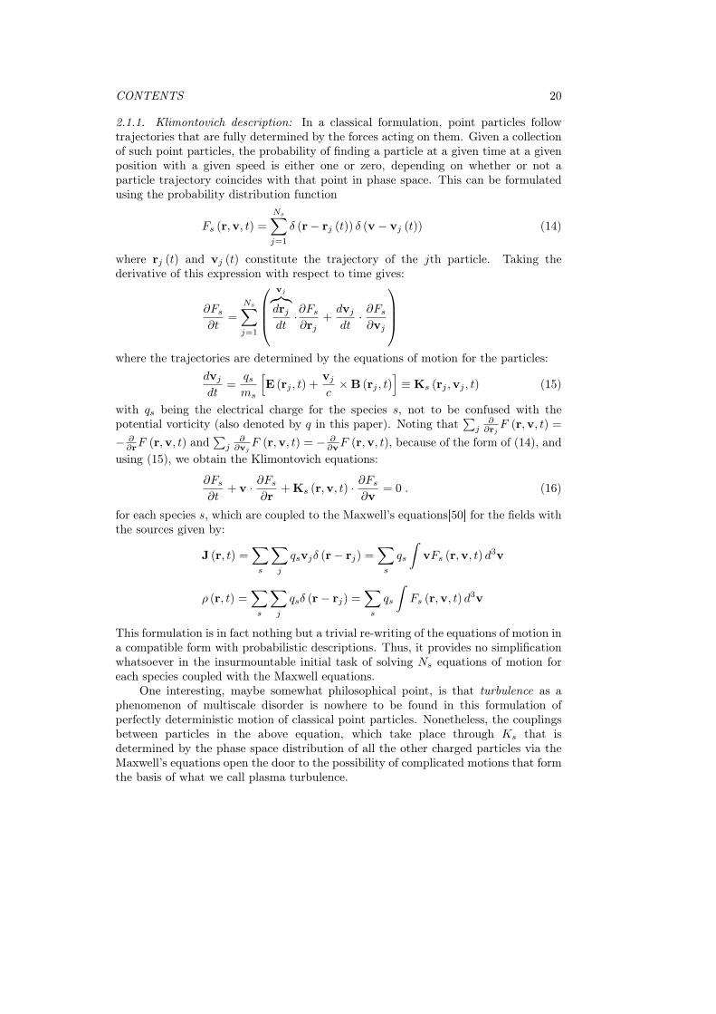
2.1.1. Klimontovich description: In a classical formulation, point particles followtrajectories that are fully determined by the forces acting on them. Given a collectionof such point particles, the probability of finding a particle at a given time at a givenposition with a given speed is either one or zero, depending on whether or not aparticle trajectory coincides with that point in phase space. This can be formulatedusing the probability distribution function
Fs (r,v, t) =
Ns∑j=1
δ (r− rj (t)) δ (v − vj (t)) (14)
where rj (t) and vj (t) constitute the trajectory of the jth particle. Taking thederivative of this expression with respect to time gives:
∂Fs
∂t=
Ns∑j=1
vj︷︸︸︷drjdt
·∂Fs
∂rj+dvj
dt· ∂Fs
∂vj
where the trajectories are determined by the equations of motion for the particles:
dvj
dt=
qsms
[E (rj , t) +
vj
c×B (rj , t)
]≡ Ks (rj ,vj , t) (15)
with qs being the electrical charge for the species s, not to be confused with thepotential vorticity (also denoted by q in this paper). Noting that
∑j
∂∂rj
F (r,v, t) =
− ∂∂rF (r,v, t) and
∑j
∂∂vj
F (r,v, t) = − ∂∂vF (r,v, t), because of the form of (14), and
using (15), we obtain the Klimontovich equations:
∂Fs
∂t+ v · ∂Fs
∂r+Ks (r,v, t) ·
∂Fs
∂v= 0 . (16)
for each species s, which are coupled to the Maxwell’s equations[50] for the fields withthe sources given by:
J (r, t) =∑s
∑j
qsvjδ (r− rj) =∑s
qs
ˆvFs (r,v, t) d
3v
ρ (r, t) =∑s
∑j
qsδ (r− rj) =∑s
qs
ˆFs (r,v, t) d
3v
This formulation is in fact nothing but a trivial re-writing of the equations of motion ina compatible form with probabilistic descriptions. Thus, it provides no simplificationwhatsoever in the insurmountable initial task of solving Ns equations of motion foreach species coupled with the Maxwell equations.
One interesting, maybe somewhat philosophical point, is that turbulence as aphenomenon of multiscale disorder is nowhere to be found in this formulation ofperfectly deterministic motion of classical point particles. Nonetheless, the couplingsbetween particles in the above equation, which take place through Ks that isdetermined by the phase space distribution of all the other charged particles via theMaxwell’s equations open the door to the possibility of complicated motions that formthe basis of what we call plasma turbulence.

CONTENTS 21
2.1.2. Vlasov equation: One problem with the Klimontovich formulation, amongothers, is that Fs (r,v, t) = Fs (r,v, t|rj ,vj , 0) depends on the initial positions andvelocities of all the particles of all species, since one needs the initial conditions forsolving the equations of motion in order to find the trajectories. Since neither thedetermination of all the initial conditions, nor the computation of all the trajectoriesis possible, a statistical description is the only option.
In order to achieve this, consider the average of Fs (r,v, t|rj ,vj , 0) over astatistical ensemble of possible initial conditions:
fs (r,v, t) = ⟨Fs (r,v, t|rj ,vj , 0)⟩The distribution function fs (r,v, t) defined this way is naturally independent ofthe initial conditions, and is formally called a “single particle distribution function”.We can write down the equation for the evolution of fs (r,v, t) by averaging theKlimontovich equation (16) over a statistical ensemble:
∂fs∂t
+ v · ∂fs∂r
+
⟨Ks (r,v, t) ·
∂Fs
∂v
⟩= 0 (17)
The Klimontovich acceleration involves only the electromagnetic fields that aresolutions of the Maxwell’s equations. Since those are linear, they can be solvedusing a response function in terms of the charges and currents, which are themselvesfunctions of the distribution function Fs. Therefore the last term in (17) describingthe correlations between particles can be reduced in two ways. If one dropscorrelations altogether, and considers only the mean fields (that is the particlesinteract with eachother only via their interactions with the collectively generated meanelectromagnetic fields), one obtains the Vlasov equation:
∂fs∂t
+ v · ∂fs∂r
+qsms
[E (r, t) +
v
c×B (r, t)
]· ∂fs∂v
= 0
in contrast, if one considers only local interactions (i.e. direct collisions), one obtainsthe Boltzman equation. In general, both of them together leads to the inclusion of acollision operator in the Vlasov equation above.
2.1.3. Freezing in laws of two-fluid description: Consider the ion equation of motion:(∂
∂t+ vi · ∇
)vi =
e
mi
(E+
vi
c×B
)− ∇Pmini
(18)
and continuity (∂
∂t+ vi · ∇
)ni + ni∇ · vi = 0
for ions.Note that (18) is isomorphic to Eqn. 1, with Lorentz force replacing the Coriolis
force. Taking the curl of the identity: ∇ (v · v) = 2v · ∇v + 2v × (∇× v) weobtain∇× [v · ∇v] = −∇× [v × (∇× v)], which can be used to rewrite (18) as:
∂
∂tΩg
i = ∇× (vi ×Ωgi ) +
1
min2i∇ni ×∇Pi (19)
where Ωgi ≡ ωi +
eBmic
is the “ion plasma absolute vorticity”, which is a sum of the ionplasma vorticity ωi = ∇×vi and the cyclotron frequency eB/mic. Since (19) has theform of a freezing in law, we can write it as
d
dt
(∇χ · Ω
gi
n
)=
1
min2i∇ni ×∇Pi · ∇χ (20)

CONTENTS 22
Considering an equation of heat of the form∂
∂tP + vi · ∇P + ΓP∇ · vi = 0
Which actually implies conservation of:(∂
∂t+ vi · ∇
)s = 0
where s = P/nΓ is the specific entropy. Now by choosing χ = s (or a function of s)causes the right hand side of (20) to vanish, resulting in the general definition of ionplasma potential vorticity as:
qi ≡
(ωi +
eBmic
ni
)· ∇s
advected by the ion velocity vi. We will see later that simply using this definitionwith a drift approximation, actually gives the correct definition of potential vorticityfor various models such as Hasegawa-Mima, Hasegawa-Wakatani or slab ITG.
Note that one can write a similar conservation law separately for the electronfluid, advected by the electron velocity
ve = vi −J
newhere J is the plasma current density. Assuming for instance that the electrons haveconstant temperature (or have a temperature proportional to their density):
qe ≡
(ωe − eB
mec
ne
)· ∇χ
where χ is a constant of motion of the electron fluid.
2.1.4. Dual PV conservation in Hall MHD If we consider the usual limit me ≪ mi,and the definition of the ve = vi − c∇×B
4πne , we can write dual freezing in laws as[51]∂tΩj = ∇× (uj ×Ωj) , (j = R,L)
with the pair of generalized vorticities and velocities defined as:ΩR = eB
mec, uR = v − c
4πne∇×B
ΩL = eBmic
+∇× v , uL = v
where v, the ion velocity plays the role of plasma velocity. Since ∇ · J = 0, theequation of continuity with the ion and electron fluids become the same with thequasi-neutrality condition ne = ni:
∂n
∂t+∇ · (nvi) =
∂n
∂t+∇ · (nve) = 0
which means that density is conserved both by ions and electrons, which allows us towrite a potential vorticity pair:
qR = 1n
eBmec
· ∇χ , uR = v − c4πne∇×B
qL = 1n
(eBmec
+∇× v)· ∇s , uL = v
such that (∂
∂t+ uj · ∇
)hj = 0 , (j = R,L)
Left fluctuations are expected to dominate the ion scales, while the right fluctuationsdominate the electron scales. This has actually been verified in a direct numericalsimulation of incompressible Hall-MHD[52].

CONTENTS 23
2.1.5. Drift-fluid description and PV conservation: For spatial scales larger than thegyro-radius and time scales slower than the cyclotron frequency, one may considerthe plasma as a reduced fluid that moves around with drift velocities. The reductionthat leads to this reduced fluid description is in fact a reduction in particle orbitsapproximating them using drift velocities. Since the dynamics of its individualelements define the nature of a “fluid” (as a continuum approximation to a discretesystem with very large degrees of freedom) the fact that the individual particlesmove in drift orbits leads to a description of a drift-fluid. Plasma in these scalesact approximately as a drift-fluid as long as local kinetic equilibrium is established.In the case where kinetic physics is important, we use a drift-kinetic descriptionwhose moments would correspond to the drift-fluid description of desired complexitydepending on the closure of the fluid hierarchy.
One interesting aspect of reduced descriptions (especially for plasmas) is thatmultiple reductions based on very different assumptions may lead to same or verysimilar reduced models even though the justifications are based on completely differenthypotheses. One example is that, one can obtain reduced MHD equations either bymaking a fluid closure (strictly justified only when the collisions dominate) and thantaking a strong magnetic field to force the system to become 2D or directly by assuminga strong magnetic field and building a fluid-like closure via the effect of the Lorentzforce dominating the dynamics [53]. The reason for that is the second step makingthe first simplifying assumption obsolete, but somehow still respecting the final result(to a certain extent). So in this sense for instance the standard MHD may be seen asan unnecessary but simplifying intermediate step.
In the same vein, the drift-fluid equations can actually be derived from two-fluidequations (which are normally justified based on collisional closures a la Braginskii).For this reason, some people call these drift-Braginskii closures. One may howeveralso derive them by directly taking the moments of the gyrokinetic equation leadingto what is known as the gyrofluid[16] description and then going to the drift limit bydropping higher order finite Larmor radius effects.
Based on this justification, we will use two-fluid equations. An asymptoticexpansion of the small parameter ω/Ωi (using the fact that the background magneticfield is very strong) leads to what is known as the drift expansion. Doing this separatelyfor ions and electrons and making the usual assumptions of quasi-neutrality andme ≪ mi leads to simple tractable fluid models[54]. However, since the startingpoint for this derivation is the two-fluid equations. The exact conservation of PV forthe two-fluid system leads to the conservation of an expanded approximate PV for thedrift-fluid, with an advection velocity given by the drift velocities.
For instance considering the dominant order ion velocity of the form vi = vE ,where vE is the E×B velocity gives directly:(
∂
∂t+ vE · ∇⊥
)([ζi +Ωi
ni
])= 0
now where ζi = ∇ × vE · b = cB∇2
⊥Φ is the parallel component of the ion plasmavorticity, and Ωi is the ion cyclotron frequency. It is interesting to note that this givesthe Hasegawa-Mima equation that will be discussed in the next section when densityis expanded as a linearly varying (i.e. in x) background and a small fluctuation aroundthat. Note that in this approach, one need not to consider the non-divergence-freehigher order correction to the plasma velocity (which is the polarization drift in thecase of magnetized plasmas) explicitly.

CONTENTS 24
2.1.6. Gyrokinetic equation and the PV: An honest description of turbulentphenomena in fusion plasmas unfortunately requires a way to treat kinetic effects. Inorder to describe kinetic evolution of plasmas under the influence of strong magneticfields, we use the gyrokinetic equation. Gyrokinetic equation in its full glory tendsto be rather complicated. However in most cases it can be written in the form of aconservation law for the guiding center distribution function Fi = Fi
(X, p∥, µ, t
):
∂
∂t
[B∗
∥Fi
]+
∂
∂X·(XFiB
∗∥
)+
∂
∂p∥
(p∥FiB
∗∥
)= 0
where µ , the adiabatic invariant is simply a label (since dµ/dt = 0). If we want todefine a quantity similar to potential vorticity, we can define:
Ni ≡ˆB∗
∥Fidv∥dµ
which is actually a normalized ion guiding center density. It becomes proportional tothe usual PV in the limit of slab with adiabatic electrons and k⊥ρs ≪ 1.
2.2. Role of turbulence in fusion plasmas, turbulent transport etc.
The possibility of transport driven by plasma microturbulence (called anomaloustransport due to historical reasons), and the difficulty this poses to the magnetizedfusion was recognized rather early on in the development of the fusion programme.Different kinds of instabilities, with different characteristics have been identified overthe years. One important class of instabilities that drive transport in tokamaks is thedrift waves[55].
2.3. Drift waves, and instabilities
The basic drift wave is a density fluctuation on top of an inhomogeneous backgrounddensity profile (see figure 9) that propagate because the radial fluctuating E × Bvelocity that this density fluctuation generates, moves the high (low) density plasmaoutward just above a density peak (hole), and low (high) density plasma inward justbelow it, leading to a movement of the density peak (hole) upward in the y direction.
For dynamics at ion scales, this wave nature relies on the adiabatic electronresponse:
n
n0=eΦ
Te(21)
which comes from the parallel (to the magnetic field) component of the electronequation of motion (Ohm’s law).
−∇∥Pe + en∇∥Φ = 0
with Pe = nTe, actually gives:
∇∥
(n
n0− eΦ
Te
)= 0 (22)
Note that (22) has two classes of solutions. The first class, can have a functionaldependence on the parallel component but obeys (21). The second class where thereis no relation between n and Φ, but both of them are independent of the parallel

CONTENTS 25
Figure 9. The basic mechanism of the drift wave. Here filled contours of densityis shown, which is the sum of a background profile decreasing in the x directionplus a fluctuating sinusoidal component, which is proportional to the fluctuatingelectrostatic potential due to the adiabatic electron response. This gives an E×Bflow as shown, which is inward just below the density maximum and outward justabove it. Since the outward flow increase the density (by carrying high densityplasma from the core) and the inward plasma decrease it, the density maximumends up moving upward.
component z. Drift waves belong to the first class, whereas zonal flows belong to thesecond.
Another interesting point of the drift wave dynamics is that if one introduces aphase difference between the density and electrostatic fluctuations (for example due tocollisions, or trapped electrons), which amounts to moving the flow pattern in figure9 downwards, since now there will be an outward motion of high density plasma atthe maximum of the density (before there was no radial motion at the peak location),in addition to the upward wave propagation there will also be an increase of theamplitude of the sinusoidal fluctuation. This is one of the mechanisms by which thebasic drift instability is excited.
The Ion temperature gradient driven (ITG) mode is an ion Larmor radius scaledrift-instability that has an overall phase speed in the ion diamagnetic direction andis driven unstable due to the ion temperature gradient. ITG can be unstable evenwith a perfectly adiabatic electron response. The collisionless, or dissipative trappedelectron modes (TEM) are ion Larmor radius scale, electron drift instabilities (i.e.they move in the electron diamagnetic direction), where the free energy source is theelectron density and temperature and the instability arises due to the non-adiabaticresponse of trapped electrons. Dissipative drift instability is an ion Larmor radiusscale electron drift instability, where the free energy source is the density gradientsand the mechanism for accessing it is the non-adiabatic electron response of passingelectrons due to collisions. Finally the electron temperature gradient driven (ETG)mode is an electron Larmor radius scale drift-instability, where the free energy source

CONTENTS 26
is the electron temperature gradient. ETG can be unstable even with adiabatic ionresponse. We will not go further into details of these different types of instabilitiesand try to focus on their common aspects.
2.3.1. The generalized Hasegawa Mima system As in the geophysical setting, onecan define a simplified potential vorticity for the plasma turbulence:
q =(ζ +Ωi)
n=
1
n
[∇2
⊥Φ
Bc+
eB
mc
]using
q ≈ 1
n0
(1− x
Ln+ n
n0
) (∇2⊥Φ
Bc+
eB
mc
)
≈ 1
n0
∇2⊥
(Φ + Φ
)B
c+1
n0
eB
mc
(1 +
x
Ln− n
n0
)whose conservation gives two equations when the fluctuating and mean componentsare separated:(∂
∂t+ b×∇Φ · ∇
)(Φ−∇2
⊥Φ)+ρsLn
∂
∂yΦ = δ
(b×∇Φ · ∇∇2
⊥Φ)
(23)(∂
∂t+ b×∇Φ · ∇
)∇2
⊥Φ = −⟨b×∇Φ · ∇∇2
⊥Φ⟩
(24)
where δ(ab)≡ ab−
⟨ab⟩, and we have used the adiabatic electron response (21) and
scaled temporal and spatial variables by Ω−1i and ρs respectively. We have also used
the dimensionless electrostatic potential eΦTe
. This system is called the generalizedHasegawa-Mima (or sometimes generalized Charney Hasegawa Mima) equations. Itsnontrivial nonlinear structure follows from the fact that the electron response to thefluctuations are adiabatic, the electrons can not respond to Φ who is independent ofthe parallel coordinate. Note that a term similar to the last term on the left hand sideof (23) is dropped from the equation for Φ, who is taken to be a function only of theradial coordinate x. However, for more general convective cells, such a term shouldbe added to (24).
2.3.2. The Hasegawa Wakatani system: Consider the potential vorticity for the driftwave problem:
q =(ζ +Ωi)
n
where ζ =∇2
⊥ΦB c as before, coupled to the equation for electron density (note that by
quasi-neutrality n = ni = ne), which can be written as:(∂
∂t+ vE · ∇
)n =
1
e∇∥J∥
we can write the vorticity equation by eliminating the density from dq/dt = 0:(∂
∂t+ vE · ∇
)(ζ +Ωi) =
(ζ +Ωi)
ne∇∥J∥

CONTENTS 27
which basically says that the plasma absolute vorticity increases with a parallel currentthat increase with the parallel coordinate since such a current profile leads to anaccumulation of electrons and thus an increase of plasma density. An increase inplasma density in turn increases the vorticity, since the potential vorticity is conserved.
The Hasagawa Wakatani system of equations follow if we use the Ohm’s Law witha finite parallel resistivity instead of the adiabatic electron response:
eη
TeJ∥ = ∇∥
(eΦ
Te− n
n0
)which gives: (
∂
∂t+ b×∇Φ · ∇
)n+
ρsLn
∂yΦ−D∇2n = c∇2∥
(Φ− n
)(25)(
∂
∂t+ b×∇Φ · ∇
)∇2
⊥Φ− ν∇4Φ = c∇2∥
(Φ− n
)(26)
where we have scaled the parallel variable by Ln and defined c ≡ 1Ωi
Te
n0L2ne
2η in additionto using the dimensionless variables of section 2.3.1 and added model diffusion termswith diffusion coefficients D and ν that are supposed to represent damping processes.
2.4. Ion temperature gradient driven instability (ITG).
While a discussion of all the various different electrostatic micro-instabilities of thedrift type in tokamaks is certainly out of the scope of this review, the ITG mode shouldprobably be mentioned as the most prominent ion Larmor radius scale instability.
The kinetic physics of the ITG mode is sufficiently complex that even the basiclinear dispersion relation, with various usual simplifying assumptions such as adiabaticelectrons and fluctuations being strongly localized to the low field side etc. requiresnumerical approach for finding the zeroes of a plasma dielectric function which hasto be evaluated numerically. Furthermore, even such a (relatively complicated)numerical calculation is well known to overestimate the growth rate of the ITG modeapproximately by a factor of two. This means the full poloidal eigenmode problemhas to be solved numerically. This is a rather fusion specific exercise and has no placein a general review such as the current one.
While its accuracy in reproducing the linear physics would be poor, a reducedfluid ITG model can be used to study the nonlinear behavior of this mode. The useof such a model may be justified retrospectively by the existence of zonal flows whichtend to weaken the balooning mode structure.
ITG requires either the parallel dynamics (cylindrical) or the curvature effects inorder to be unstable. We start with the PV budget (11) as in the rotating convectionproblem:
dq
dt= Pq −Dq
where, we write the dissipation as Dq = −ν∇2⊥q.
The potential vorticity for the simple slab ITG system can be defined as
q =(ζ +Ωi)P
1/Γ
n

CONTENTS 28
considering P = P0
(1− x
LP+ P
P0
), n = n0
(1− x
Ln+ n
n0
), and ζ ≈ c
B∇2Φ:
q ≈ P1/Γ0
n0
[c
B∇2Φ + Ωi
(1−
[n
n0− x
Ln
]+
1
Γ
[P
P0− x
LP
])]which basically is equivalent to q = ∇2Φ − n + P
Γ in dimensionless form when theconstant is dropped. The conservation of potential vorticity implies:(
∂
∂t+ b×∇Φ · ∇
)[∇2Φ− n+
P
Γ
]+
(ρsLn
− ρsΓLp
)∂Φ
∂y= 0
2.5. General Formulation based on Potential Vorticity advection
In all the systems above, the problem can be reduced to a potential vorticity equationcoupled to some other equations through the baroclinic (or other) drive term.
For instance the inviscid limit of the Hasegawa-Wakatani equations given above,can be written as two equations, one for potential vorticity advection, and the other fordensity. The PV equation is “independent” of the density equation (i.e. we can solve forPV without knowing the value of the density), however the density equation involvesthe electrostatic potential (i.e. the stream function). The electrostatic potential canbe written as a function of PV and the density [i.e. Φ = ∇−2 (q + n), which is a non-local integral and thus includes the boundary conditions as well]. This is known as theproblem of invertibility and is trivially solved in the adiabatic limit (since in this limitΦ = n). However in the general case, the invertibility becomes a more complicatedproblem since now given q, we need to solve an integro-differential equation [i.e. Eqn25 with ∂yΦ replaced by ∂y∇−2 (q + n)] to obtain n and hence n, which we can useto obtain Φ. While this complicates the full problem, in principle the fact that it isdoable allows us to focus on the PV dynamics, which is nicely decoupled from densityor any other quantity as long as there is no drive. In contrast, the case of rotatingconvection where the coupling to the temperature equation is via the baroclinic term,or the case of ITG where the coupling is via the temperature gradient drive are caseswhere the PV equation is only partially decoupled and we have a quasi-conservationinstead of an exact conservation.
Note that mesoscale flows defined as v = b×∇Φ in section 2.3.1, and mesoscalepotential vorticity which can be denoted by q, can be added to all the simplesystems that are considered above, while we avoided adding them explicitly to avoidcumbersome notation.
The general structure of the potential vorticity equation in this case becomes:(∂
∂t+ b×∇Φ · ∇
)q+b×∇Φ·∇ (q0 + q)+δ
(b×∇Φ · ∇q
)= 0(27)(
∂
∂t+ b×∇Φ · ∇
)q + b×∇Φ · ∇q0 +
⟨b×∇Φ · ∇q
⟩= 0 (28)
note that we recover (23) and (24) by using q = ∇2Φ− Φ and q = ∇2Φ. One can addinjection and dissipation to these in order to apply them to cases where there is onlya quasi-conservation. Note also that the middle term in (28) usually drops when weconsider flows that are perfectly zonal.

CONTENTS 29
3. Formation of zonal flows
Zonal flows form in all the physical systems discussed in the previous sections throughsimilar mechanisms. The fluctuations that are driven unstable by some mechanismprovide the Reynolds stress, which drive large scale flows, which in turn modify theunderlying turbulence that is driving them. There are different ways to express thisboth in common language and in mathematical formulation. in particular differentaspects of this phenomenon of turbulence self-regulation via zonal pattern formationare described using different mathematical frameworks.
3.1. Zonal Flows and Potential Vorticity(PV) mixing.
Various problems in geophysical fluid dynamics, plasma physics, and laboratoryexperiments of rotating convection can be formulated using a potential vorticity quasi-conservation, where the injection is via the baroclinic, or temperature gradient driveninstabilities and the dissipation is due to small scale stresses. Therefore general rulesabout the tendencies of potential vorticity dynamics are very useful for understandingthe common features of such systems.
One rather interesting, general observation of potential vorticity dynamics is thatas long as the initial configuration has closed contours of time averaged potentialvorticity [i.e. ⟨q⟩ ≡ q0 + q in the formulation of (27-28)], the final state will consistof homogenized patches of potential vorticity connected by large gradients. Similarconclusion can also be drawn for contours of mean flow (streamlines), since to thelowest order these two are functionally related. This can be shown in different ways[1]here we only mention the demonstration using the integral around a closed potentialvorticity contour.
First note that the basic background steady state solution of (28), suggests that
b×∇Φ · ∇ ⟨q⟩ ≈ 0
which means that to the lowest order, there is a functional relation between the meanpotential vorticity and the mean electrostatic potential:
⟨q⟩ = Q(Φ)+O (ϵ) (29)
Note also that for any function f , the integral over an area A enclosed by a meanstreamline ˆ
A
b×∇Φ · ∇fds =˛C
b×∇Φf · dℓ = 0 (30)
where C is the closed contour around the streamline [i.e. dℓ = ∇Φdℓ/∣∣∇Φ
∣∣].Using this and (28), we can write:ˆ
C
⟨b×∇Φq
⟩· dℓ ≈ 0 (31)
in the steady state. Now using an eddy viscosity hypothesis:⟨b×∇Φq
⟩i∼ −κij
∂
∂xj⟨q⟩
And the perturbation expansion (29), we can write
−∂Q∂Φ
ˆC
κij∂
∂xiΦ
∂
∂xjΦ
dℓ∣∣∇Φ∣∣ ≈ 0

CONTENTS 30
which implies that as long as κij is positive ∂Q
∂Φ≈ 0 for any closed streamline. This
means that the potential vorticity does not vary from one streamline to another ona such a closed contour, which means that the steady state solution of the problemdefined by (27) and (28) is simply:
⟨q⟩ = q + q0 = const. +O (ϵ)
in a region where the initial condition contained a closed contour of mean potentialvorticity.
However since this is in opposition to the background variation of the potentialvorticity for example due to background density gradient in the drift wave problem.The flat region of PV would have to be connected to the next flat region by a stronggradient. When many of such regions are connected, the result is what can be calleda PV staircase.
Notice that the nonlinear term vanishes for a homogenized PV profile. There isa close analogy between the homogenization of the PV and the phenomenon of fluxexpulsion in MHD and eventually to the phenomenon of dynamic alignment whichleads to generation of large regions of aligned or counter-aligned velocity and magneticfield profiles which are connected by sheets or filaments where the alignment changesrapidly.
3.1.1. Rhines Scale and its applicability to fusion plasmas. The Rossby waveturbulence in the atmosphere as described by the Charney equations is rather similarto the 2D turbulence described by the Euler equations. This is true in particular forsmall scales where the equation basically becomes an Euler equation apart from theβ effect.
If one compares the linear and the nonlinear terms in (10), noting that thenonlinear term scales dimensionally as U2/L2 and the linear term as β′U it is clearthat for a given β′ and U , the two terms balance each other at a length scale given indimensional units by:
LR ≡(U
β
)1/2
or a wave-number kR ≡ (β/U)1/2 , where U is interpreted as a characteristic (rms)
velocity of the fluid (sometimes a rather arbitrary factor such as 2 or π may beintroduced at the denominator). For scales larger than this scale (wavenumberssmaller than kR), the linear term which represents the β effect will dominate, andwave turbulence, which leads to formation of zonal flows will result. Whereas forsmaller scales (i.e. wave-numbers larger than kR), the nonlinear term dominates andfully developed 2D turbulence will result. Notice that if the Rossby deformation radiusR =
√h0gf
−10 is already much larger than this critical length scale, we can treat small
scale turbulence by using Euler equation directly.The usual description of fully developed 2D turbulence involves a dual cascade
where the Enstrophy cascades forward and the Energy cascades inversely. Therefore,another way to view the Rhines scale is as a scale where the 2D inverse cascadeterminates since the turbulence changes character beyond this scale. Therefore it iscommon to talk about the “arrest” of inverse energy cascade at the Rhines scale, eventhough it is open to debate whether the 2D turbulence really generates a local inversecascade or if this inverse cascade is really arrested at the Rhines scale.

CONTENTS 31
-1
-0.5
0
0.5
1
-1 -0.5 0 0.5 1
Figure 10. Anisotropic Rhines scale for Drift Wave turbulence. Inside thecurve, the turbulence has a wave-like character and interactions with the zonalflows dominate, outside it has the character of a classical fully developed 2Dturbulence.
When the dispersion relation is anisotropic as in the case for Rossby or drift waves,the Rhines scale generalizes to a curve in k space inside of which the interactions withzonal flows dominate. This can be demonstrated for drift waves as follows (see [56]for the Rossby wave version):
u2rmsk2R = ω2 =
(ρsLn
)2 ρ2sk2Ry
(1 + ρ2sk2R)
2Ω2i
(ρskR)2 (
1 + ρ2sk2R
)2=
(ρsLn
)2(sinαR)
2
(eΦrms/Te)2 (32)
note that we have defined sinαR ≡ kRy/kR. The curve is represented in figure 10.Inside this curve, weak wave turbulence and therefore wave-like modes interactingmainly via the zonal flows dominate, and outside the curve we have a classical fullydeveloped 2D turbulence. Since the energy is usually injected inside the curve fordrift instabilities (which usually has a most unstable mode with finite ky and kx ≈ 0),and couples to zonal flows which fall outside the curve, the role of the Rhines scalein drift-wave turbulence is quite different from the arrest of the 2D inverse cascade
picture. Note that as an order of magnitude (eΦrms/Te)2 ∼
(ρs
Ln
)2in drift wave
turbulence (i.e. the mixing length estimate).While the applicability or the importance of the Rhines scale to fusion plasma
turbulence may be questionable, the curve given in Figure 10 can be interpreted as theboundary between anisotropic turbulence at “large” scales and the isotropic turbulenceat “small” scales. When the energy is injected within the above curve, it will excite adrift wave which has the form of a streamer (i.e. kx ≪ ky mode), this mode couplesnaturally to an isotropic mode (with kx ∼ ky, sometimes called a Kelvin-Helmholtz-like mode, but we think that this terminology is very misleading) and a zonal mode.The interaction in a fusion device is actually a 4-wave interaction where the twosatellites of the primary pump mode (i.e. the streamer) couple to give the zonal

CONTENTS 32
mode. We will discuss how this can be described in the framework of modulationalinstability in the following sections.
However note that as the energy goes to the zonal flow, the zonal flow transferssome of this energy to a smaller (or larger) scale kx ∼ ky mode and a smaller (orlarger) scale streamer-like mode. Sometimes called a tertiary instability. Howeversince the smaller scale streamer that is driven by the “tertiary instability” then drivessmaller scale zonal flows leading to a cascade of enstrophy through the k-space viathese particular triads, it is in fact simply a part of an hierarchy of interactions. Wethink that within the context of turbulence calling it an “instability” is misleadingunless one sees each step in the cascade as an instability of the previous scale. Incontrast it is clear that for single wave-packet whose characteristics actually evolve intime, the tertiary instability has a clear meaning.
3.1.2. Rhines Scale vs. Mixing Length vs. Critical Balance There are variousexamples in the literature where people consider the balance between the linear andthe nonlinear terms as we have discussed above to define the Rhines scale. Themixing length idea commonly used in fusion to estimate the fluctuation level is indeeda balance between the linear and the nonlinear terms. For instance for the Hasegawa-Mima case:
ρsLn
ρs∂
∂y
(eΦ
T
)≈ ρ4sb×∇
(eΦ
T
)· ∇∇2
⊥
(eΦ
T
)which gives (for ρsk⊥ ∼ ρsky ∼ 1 which is roughly true for the most unstable mode):
eΦ
T∼ ρsLn
this is the basic mixing-length estimate of the fluctuation level for drift-waveturbulence. A more detailed version can be used to determine the maximum of theturbulence k-spectrum by arguing that the maximum occurs when the linear growthrate is balanced by the nonlinear decorrelation rate (i.e. eddy damping):
γk ≈ Dnlk k
2⊥
where Dnlk ∝
∣∣∣ eΦk
T
∣∣∣2 is the nonlinear diffusion coefficient that appears in turbulentfluxes of density and particles[57]. The maximum of the spectrum can be obtained bysolving:
max
∣∣∣∣∣eΦk
T
∣∣∣∣∣2 ≈ max
(γkk2⊥
)for k. Since the functional form of γk can in principle be obtained maximizing γk/k2⊥one obtains the mixing length maximum of the spectrum. It is interesting to notethat this seems to work rather well for turbulence in tokamak plasmas even withcomplicating effects of curvature, magnetic shear etc. The reason is probably thatmost of the complicating effects change the form of γk in this argument, but do notchange the fact that the γk is balanced by an effective turbulent diffusion near themost unstable mode. Note that while one uses the same basic idea of balancing linearand nonlinear terms, the mixing length considers the energy budget (so the energyinjected by the linear instability is equal to the energy extracted by the nonlinear

CONTENTS 33
transfer), whereas the Rhines scale argument is based on a comparison between theeddy turnover rate and the wave propagation in the original equation.
Yet another famous balance between the linear and the nonlinear terms is theso-called critical balance[58] in 3D MHD turbulence. The idea is very similar to howone obtains the Rhines scale but considering parallel propagating Alfvén waves with afully developed 2D perpendicular spectrum. By balancing the Alfvén wave transit ratein the parallel direction with the eddy turnover rate in the perpendicular direction,one obtains:
vAk∥ ≈ u (k⊥) k⊥
Notice that in standard 3D MHD there is no process which would break the isotropyon the perpendicular plane (i.e. kx vs. ky), however there is a rather important sourceof anisotropy in the parallel vs. perpendicular directions. Since the spectral energydensity in the perpendicular direction for a 2D forward cascade is E (k⊥) ∝ ε2/3k
−5/3⊥
or u (k⊥) ∼ E (k⊥)1/2
k1/2⊥ ∝ ε1/3k
−1/3⊥ , the critical balance gives the relation:
k∥ ∝ ε1/3
vAk2/3⊥
This is usually interpreted as a strongly anisotropic spectrum with k∥ following thek⊥ cascade scale by scale until it reaches the critical balance. It can be generalizedfor an arbitrary dispersion relation by replacing vA with the parallel phase velocityvph∥ (k). The idea can be applied to various systems with parallel propagating waves.
3.1.3. PV and its importance in DW/ZF dynamics. As discussed above, a number ofplasma and geophysical fluid dynamics models can be formulated using a descriptionbased on potential vorticity evolution. Advection of potential vorticity, coupled toother equations such as that of entropy density or pressure via the baroclinic term orvia curvature effects when there are additional sources of free energy. Notice howeverthat in general the quadratic quantity that is conserved by the nonlinear dynamics ofco-evolving drift waves and zonal flows, as described for instance by (23) and (24), isthe potential enstrophy.
W ≡⟨q2⟩=⟨|q|2⟩+ q2 =
⟨∣∣∣(1−∇2)Φ∣∣∣2⟩+
⟨∣∣∇2Φ∣∣2⟩
In other words the nonlinear system described by (23) and (24), the zonal flows andthe drift waves exchange potential enstrophy and not energy. So it is the potentialenstrophy that is conserved between the drift waves and the zonal flows, since it is thepotential vorticity that is advected. However local interactions among the drift wavesstill conserve energy and enstrophy leading to a dual cascade.
3.1.4. Forward Enstrophy cascade and ZF formation. One interesting point is thatwhile it is common to talk about zonal flow formation informally as a process of“inverse cascade”, in reality the anisotropic mechanism that leads to the formationof zonal flows does not really have the character of a local cascade where the energymoves to larger and larger scales. The mechanism can be described better as a nonlocalinteraction in k-space where the zonal flow acts on all scales diffracting the fluctuationsto smaller and smaller wave-numbers (see figure 11).
From a spatial, ’pattern formation’ point of view, the same process can beexplained by looking at the dispersion relations for drift or Rossby waves. Consider

CONTENTS 34
Figure 11. Forward potential enstrophy cascade mediated by large scale flowstructures.
the setup in figure 12, for Rossby waves as the first example. The basic Rossby wavehas a mainly westward phase motion, with a phase velocity given by:
vph = −β′kxk4
k
while its latitudinal group velocity, vgx , can be in either direction, its meridional groupvelocity, vgy, is in the opposite direction to its meridional phase velocity, making it abackwards wave in the meridional direction:
vgy =∂
∂ky
(−β
′kxk2
)=
2β′kxkyk4
Similarly for drift waves the main phase velocity propagation direction is counter-clockwise in the geometry of figure 12 if the magnetic field is in the out of planedirection. The radial group velocity
vgx =d
dkx
[ρ∗Ln
ky(1 + k2)
]= − ρ∗
Ln
2kxky
(1 + k2)2
which is also backwards with respect to its radial phase propagation (i.e. vphx =ρ∗Ln
kykx
(1+k2)k2 ). Note that while Rossby waves carry negative wave momentum awayfrom the stirring region, the drift waves carry positive wave momentum towards thestirring region resulting in the same basic effect of momentum convergence towardsthis region.
One very interesting point is that if an infinitesimal velocity shear which hasthe profile given in figure 12 is introduced, the sheared flow leading to a tilting of theeddies resulting in a radial (meridional in the case of Rossby waves) group propagationwhich leads to momentum convergence towards the maximum of the flow.
3.2. The Wave-Kinetics formulation
Self-regulating drift/Rossby wave turbulence, can be described using the wave kineticequation in a weakly inhomogeneous medium[59, 60, 61]:
∂
∂tNk (X, t) +∇k ·
[(ω −V · k
)∇XNk (X, t)
]−∇X ·
[(ω −V · k
)∇kNk (X, t)
]= C ′ (Nk, Nk) (33)
where Nk is the wave quanta of the drift waves. The weak inhomogeneity describedpartly by the dispersion relation and partly by the mean flow V above can be

CONTENTS 35
Figure 12. Simple mechanism for the zonal flow reinforcement.
coupled to the slower time scale evolution of the zonal flows using a scale separationapproach. Notice that it is also possible to obtain the wave kinetic formulation, andderive explicit expressions for the diffusion coefficients using a Lagrangian correlationsapproach[62, 63].
When considered by itself the wave-kinetic equation describes the evolution ofhigh frequency drift waves that move around in a medium whose optical index ofrefraction is determined by the zonal shearing. Recall that the WKB equations canbe written as
dx
dt=
∂
∂k
(ωk −V · k
)and
dk
dt= − ∂
∂x
(ωk −V · k
)which is the basis for the interpretation of (33) as a “kinetic” equation. Notice thatsince zonal flows are narrow banded flow structures, they play the role of wave-guidesfor drift waves.
The wave kinetic formulation of drift-wave zonal flow interaction is a very powerfultool. As discussed in detail in Ref. 34, a quasi-linear calculation, based on the wave-kinetic formulation (i.e. using Nk = ⟨Nk⟩+ δNk where δNk is a perturbation) can beused to estimate the zonal flow “growth rate” (i.e. the rate at which the zonal flowsare driven by drift waves):
γq [Wk] = −2q2c2s∑k
k2yρ2s
(1 + k2ρ2s)2R (k, q) kx
∂
∂kxWk
where Wk =
⟨(1 + ρ2sk
2)2 ∣∣∣Φk
∣∣∣2⟩ is the drift wave potential enstrophy density.
Remarkably, the general form of the coupled quasi-linear system of equations thatresult:
∂
∂tWk − ∂
∂kr
[Dk
∂
∂krWk
]= γkWk − ∆ωk
N0W 2
k (34)

CONTENTS 36
∂
∂t|Φq|2 = γq [Wk] |Φq|2 − γd |Φq|2 − γnl
[|Φq|2
]|Φq|2 (35)
A formal statistical calculation based on the direct interaction approximation betweendisparate scales for the generalized Hasegawa-Mima system gives essentially the sameresult also64. Notice that the equations (34) and (35) already suggest
(i) that the turbulence drives zonal flows via γq.(ii) that the zonal flows contribute to the forward enstrophy cascade by refracting
the drift waves towards smaller kr.
adding the zonal flow damping, we have roughly all the ingredients for a spectralpredator-prey dynamics as described in figure 11.
3.3. Modulational instability framework
Assuming that the spatio-temporal dynamics of large scale flow structures issufficiently slower than that of drift/Rossby wave turbulence, one can use themodulational instability framework. The complete framework can actually bedeveloped from a Hamiltonian description of nonlinear waves, for which there arealready very good books and reviews [65, 66]. Since, the purpose of this paper isto review physical mechanisms, we limit ourselves to a discussion of the modulationinstability and discuss the formulation by A.C. Newell [67]. Consider the nonlinearsystem
L (∇, ∂t, R)ϕ = NϕMϕ (36)
where L, N and M are operators representing linear terms and nonlinear couplingsrespectively, and R represents a parameter that determines the stability condition (e.g.the Rayleigh number for the problem of convention). We obtain the linear dispersionrelation for given R by linearizing (36):
L (ik,−iω,R) = 0 (37)
where ω = ωk ≡ ωrk + iγk is the complex frequency. One can obtain the stabilitycondition by substituting ω = ωk (R) and setting γk = 0, and solving for R = Rc (k)instead.
In many problems in nature there is a critical scale (the most unstable mode)at which the net energy production has a maximum because the energy productiondecreases towards larger scales, and the dissipation increases towards smaller scales.This implies that Rc (k) has a minimum at this point. Thus, when the controlparameter R is close to, but slightly above its critical value
R = Rc
(1 + ϵ2χ
)only a small subset of modes around the most unstable mode are excited [i.e.kc ±O (ϵ)]. This allows us to consider a wave whose amplitude is slowly modulated:
ϕ = Φ(X,T , τ
)eik·x−iωrk t + c.c.
where Φ(X,T, τ) is the modulated complex amplitude, using the reductiveperturbation theory:
ϕ = ϵ(ϕ0 + ϵϕ1 + ϵ2ϕ2 + · · ·
)with a basic scale separation assumption, which can be regarded as a Taylor seriesexpansion of the operator L = L0+ ϵL1+ ϵ
2L2+ · · ·, around the point (∇, ∂t, Rc) to a
CONTENTS 37
neighboring point(∇+ ϵ∇, ∂t + ϵ∂T + ϵ2∂τ , Rc
[1 + ϵ2χ
])in the operator space. For
example
L1 =
(∂L0(ik,−iω,R)
∂(−iω)∂T +
∂L0(ik,−iω,R)∂(ik)
· ∇)
=∂L0(ik,−iω,R)
∂(−iω)(∂T+vg·∇)(38)
where we have used the fact that∂
∂kL0(ik,−iω,R) = −∂ω
∂k
∂
∂ωL0(ik,−iω,R)
which can be obtained by differentiating the dispersion relation (37). Note that (38)corresponds to the group motion of the envelope modulation and can be eliminatedby transforming to a frame of reference moving with the group velocity.
Similarly
L2 = −1
2
∂2L0
∂ω2∂TT+
∂2L0
∂ki∂ω∂T∂i−
1
2
∂2L0
∂ki∂kj∂i∂j+i
∂L0
∂ω∂τ+
∂L0
∂RRχ(39)
substituting the following relation, which can be obtained by taking the secondderivative of the dispersion relation with respect to k:
−1
2
∂2L0
∂ki∂kj=
1
2
∂2ω
∂ki∂kj
∂L0
∂ω+
1
2
∂ω
∂ki
∂ω
∂kj
∂2L0
∂ω2+∂ω
∂ki
∂2L0
∂kj∂ω+
1
2
∂2R
∂ki∂kj
∂L0
∂R(40)
and using the transformation to the group velocity frame that was used to eliminateL1 (i.e. ∂T = − ∂ω
∂ki∂i), we note that the first and second terms of (39) are canceled
by the second and the third terms on the right hand side of (40) respectively. Thisleaves:
L2 = i∂L0
∂ω∂τ +
1
2
∂2ω
∂ki∂kj
∂L0
∂ω∂i∂j +
1
2
∂2R
∂ki∂kj
∂L0
∂R∂i∂j +
∂L0
∂RRχ (41)
which is to be balanced by the nonlinear terms. The exact form of the resultingequations depend on the details of the nonlinear saturation mechanism that balancesthe envelope modulations that can be described in general using the above formalism.The Envelope equation, including the lowest order nonlinear terms takes the form
L2Φ0 ≈ N0Φ0M0Φ0
The simplest possible example that results in various physical problems is the socalled nonlinear Schrödinger equation, which takes the form:
i∂τΦ+1
2
d2ω
dk2∂2
∂x2Φ+ λ |Φ|2 Φ = 0
where λ is the lowest order coefficient for the perturbation expansion of the nonlinearterm. The nonlinear Schrödinger equation is common to a number of interestingphysical problems, and its implications are profound. Another thing that is veryremarkable about this equation is that, it has actually been solved using the inversescattering method, which were later on developed into a methodology for solvingsimilar equations. However here we only use it as an example to the large class ofpossible amplitude equations that can be obtained from the modulational instabilityframework and refer the reader to the well written books and review papers on thesubject.

CONTENTS 38
3.3.1. Amplitude equations and their application to basic zonal-flow/drift-wave systemConsider the nonlinear system (23-24) which describes the coupled evolution of simpledrift-waves and zonal flows. We can write (23) in the form:
LΦ = −b×∇Φ · ∇(Φ−∇2
⊥Φ)+ δ
(b×∇Φ · ∇∇2
⊥Φ)
where the linear dispersion relation follows from:
L0 (ik,−iωk) = −iωk
(1 + k2
)+ρsLn
ky = 0
which gives:∂
∂ωkL0 (ik,−iωk) = −i
(1 + k2
)Note that for this problem, there is no R, since the basic linear dispersion relation isalways stable.
Using the reductive perturbation method described above, considering zonalmodulations, and flows (i.e. ∂Y → 0) and assuming further that the zonal electrostaticfield varies roughly at the same scale at which the envelope is modulated [i.e.Φ0 = Φ0 (X,T, τ) e
i(k·x−ωt) and Φ = Φ(X,T )], we can write for L2 from (41):(i∂τ +
1
2
∂2ω
∂kx∂kx∂XX
)Φ = kyΦ∂XΦ (42)
which is then coupled to
(ϵ∂τ − vgx∂X) ∂XXΦ = 2kxky∂XX |Φ|2 (43)
Note that a scaling Φ ∼ O (ϵ), Φ ∼ O (ϵ) is suggested if the term on the right handside of (42) is to be of the same order as the term on the left hand side, while thegroup velocity term in (43) is to be of the same order as the term on the right handside. In this case we can solve (43) by neglecting the the higher order ϵ∂τ term andsubstitute the result into (42), which gives:
i∂τΦ+1
2
∂2ω
∂kx∂kx∂XXΦ+
2kxk2y
vgx|Φ|2 Φ = 0 (44)
which is again the nonlinear Schrödinger equation (NLS), which we write as
i∂τΦ+ β∂XXΦ+ α |Φ|2 Φ = 0 (45)
where
β ≡ 1
2
∂2ω
∂kx∂kxand α ≡
2kxk2y
vgx(46)
Consider the following perturbed homogeneous solution:
Φ = (Φ0 + δΦ) eiα|Φ|2τ
which, without the δΦ is a homogeneous plane wave with a nonlinear frequency shift.Looking at the linear stability of δΦ ∼ δΦ0e
i(qxX−ωZτ), one obtains the dispersionrelation:
ω2zf = β2q4x − 2αβq2x |Φ0|2 .
The instability condition for this dispersion relation is basically that
q2x < 2α
β|Φ0|2

CONTENTS 39
when the mode is unstable, we can write:
γzf (qx) =
√2αβq2x |Φ0|2 − β2q4x
which allows us to compute the most unstable zonal mode, [i.e. by setting γ′zf (qx) =0]:
q2x =α
β|Φ0|2 (47)
and with this the growth rate of the most unstable mode:
γzf (qx) = |α| |Φ0|2 =cs |ky|
(1 + ρ2sk
2)2
ρs/Ln
∣∣∣∣eΦ0
Te
∣∣∣∣2in dimensional form.
It is interesting to note that, the modulational instability framework, defines aspecific characteristic “most unstable” wave-number for the zonal flows [i. e.(47)].While the final “steady state” (if there ever is a steady state) value of the zonal flowwave-number depends also on the way it is dissipated, which we will discuss in Section4, the most unstable wave-number would give an indication about the characteristicradial size of the zonal flows. It is interesting to note that as to the knowledge ofcurrent authors, this was never used as a basis for comparison, at least in fusionexperiments.
3.4. Pattern selection in electron scales by modulational instability
Using the general framework of modulational instability, we consider a two field modelof small scale drift turbulence driven by electron temperature gradient (ETG). Bothbecause it was done initially for this system and due to the its direct similarity to therotating convection problem discussed in Section 1.3. Here we also demonstrate theapplication of the modulational instability framework to the question of 2D patternselection in plasma turbulence. We consider a reduced fluid ETG system as a workingmodel:
(∂t + z×∇Φ · ∇)(1−∇2)Φ + ∂y(Φ + P ) + ν∇4Φ = 0 (48)
(∂t + z×∇Φ · ∇)P − χ∇2P − r∂yΦ = 0 (49)
where the following dimensionless drift wave variables are used:
Φ → eϕTiϵ∗i
, P → ϵBPe1
ϵ2∗iPi0, t→ Ωeϵ∗it, x → x/
√τρe
ϵ∗i =√τρe
Ln= v∗i
cse, ϵ∗e = −
√τρe
Lpe= v∗e
cse, ϵB =
√τρe
LB= vB
cse, r = ϵBϵ∗e
ϵ2∗i
and τ = Ti/Te. In order to apply the modulational instability framework, we separatethe fluctuations and mean flows/fields. The mean flow equations, dropping thedissipative terms, can be written as
∂T (1−∇2)Φ + ∂Y (Φ + P ) =⟨z×∇Φ · ∇∇2Φ
⟩(50)
∂T P − r∂Y Φ =⟨z×∇P · ∇Φ
⟩(51)
and the two equations for the fluctuations can be combined as:[∂t
(∂t(1−∇2) + ∂y
)+ r∂yy
]︸ ︷︷ ︸L(∂t,∂y ,∂x)
Φ−(z× k · ∇)((ω(1 + 2k2
y)− rky)Φ− kyP
)︸ ︷︷ ︸N(Φ,P )
Φ = 0 (52)

CONTENTS 40
by dropping the direct interactions between fluctuations and dissipation.The Reynolds stress for a modulated monochromatic wave in general can be
written as:⟨z×∇Φ · ∇∇2Φ
⟩≈ 2(z×k · ∇)(k · ∇) |Φ|2 + (z×k · ∇)(∇ · J)− (k · ∇)(∇× J)z(53)
where,
J = i(Φ∇Φ∗ − Φ∗∇Φ)
is the Schrödinger intensity flux density, and Φ is the complex amplitude. Similarlyfor the advection of pressure,⟨z×∇P · ∇Φ
⟩≈ ∇ · (z× ik [Φ∗P − P ∗Φ] + z× [Φ∗∇P − P ∗∇Φ]) . (54)
The phase difference between Φ and P can be calculated from (49), by including slowmodulations. When we consider a particular perturbation expansion (53) and (54)will be further simplified.
It is easy to see, from (52) that the linear dispersion relation has two solutions,and the unstable mode has a maximum at kx = 0. This means that the monochromaticdrift-wave around which we perform the modulational instability has kx = 0 but finiteky.
3.4.1. Initially Isotropic modulations In order to see what kind of elongated patternsform among zonal flows with ∆X ≪ ∆Y , streamers with ∆X ≫ ∆Y , or isotropicconvective cells with ∆X ∼ ∆Y , we start the analysis with isotropic modulations andsee in which direction the system evolves. The amplitude equation in this case can bewritten as:
i∂τΦ+1
2
∂2ω
∂k2y∂Y Y Φ+
1
2
∂2ω
∂k2x∂XXΦ+ αk2y∂XX(|Φ|2)Φ = 0 (55)
It is also possible to rewrite this with the scalings X → X/√
|βx|, Y → Y/√
|βy|,Φ → (ky
√|α/βx|)Φ, where βx = (1/2)∂2ω/∂k2x and βy = (1/2)∂2ω/∂k2y, and replacing
Φ → Φ∗ if βx < 0, which gives:
i∂τΦ+ ∂Y Y Φ+ ∂XXΦ+ σ∂XX(|Φ|2)Φ (56)
This scaling uses the fact that the signs of βx and βy are the same. Here σ = ±1 isthe overall sign of (α/βx), where σ = −1 corresponds to an attractive nonlinearityand σ = +1 to a repulsive one. The total Hamiltonian for (56):
H =
ˆdV[|∂XΦ|2 + |∂Y Φ|2 +
σ
2
(∂X(|Φ|2
))2] (57)
is conserved. Following Talanov, we write the evolution equation for the radial andpoloidal variance (defined as
⟨X2⟩=´X2|Φ|2dXdY and
⟨Y 2⟩=´Y 2|Φ|2dXdY
respectively):
d2⟨X2⟩
dt2= 4H + 4
ˆ [σ(∂X |Φ|2)2 + (|∂XΦ|2 − |∂Y Φ|2)
]dXdY (58)
d2⟨Y 2⟩
dt2= 4H + 4
ˆ [|∂Y Φ|2 − |∂XΦ|2
]dXdY (59)
As these are explicit differential equations for the second derivatives of thesequantities (akin to acceleration), one may qualitatively interpret them as Newton’s

CONTENTS 41
equations of motion. For H < 0, which is possible for σ = −1, the total varianceV is always ’pulled’ towards zero, leading to a collapse. However it is easy to seethat for H < 0 Vx − Vy is always ’pulled’ towards the negative axis. This means⟨X2⟩
is always ‘pulled’ more strongly than⟨Y 2⟩. Since an initially isotropic state
corresponds to⟨X2⟩∼⟨Y 2⟩, one arrives at the conclusion that the final state will
have⟨X2⟩≪⟨Y 2⟩
or ∂X ≫ ∂Y . Notice that H < 0 is a condition on the initial datathat allows the finite time singularity formation.
The collapse of the initial data to a singular layer in the perturbation analysissuggests that the wave amplitude becomes larger and ∂X becomes smaller thanit is assumed in the perturbation expansion corresponding to the initial isotropicmodulation. The complete evolution of an initially isotropic amplitude modulationcan be seen in figure 13. The perturbation expansion breaks down as the systemcollapses in the radial direction, resulting in a poloidally elongated (i.e. ∂X ≫ ∂Y )modulation (and flow) structure. However, we can continue the analysis by choosinga new scaling.
3.4.2. Further anisotropic evolution An equation describing the further evolution ofthe structure in the limit ∂X ≫ ∂Y may be derived similarly to the isotropic case. Themain problem is that if the scaling is such that ∂Y ∼ ∂2X , one can no longer neglect thedivergence of intensity flux density term ky(∂x∇·J) in the calculation of the Reynoldsstress. It is possible that this term nonlinearly damps the zonal flow, balancing theself focusing tendency. Thus, the critical scaling ∂X ∼ O(ϵ1/4), corresponds on thescale at which the collapse possibly stops (see figure 13). Using ϵ∗i as a crude estimatefor ϵ we get ∆X ∼ ρ
3/4es L
1/4n for the radial scale of the final meso-scale structure. If
this is the zonal flow (i.e. no breakup into smaller scale structures occurs), then thiswould be the radial size of the zonal flow. However, as mentioned before, it is alsopossible that breakup into smaller scale structures occurs, then, this estimate wouldcorrespond to the radial size of these ‘small scale’ structures resulting from a tertiaryinstability.
Before the critical scaling however there is an intermediate scaling. Since thiscorresponds to a poloidally collapsed state of an initially isotropic field, the scalingof ∂Y should be kept as before [i.e. ∂Y ∼ O(ϵ1/2), ∂X ∼ O(ϵ1/3),kx ∼ O(ϵ1/2) andky ∼ O(1)] avoiding the critical scaling ∂x ∼ O(ϵ1/4), in order to be able to neglectthe divergence of the intensity flux density term. This, in turn, results in a scaling ofthe mean field as Φ ∼ O(ϵ1/3), and time as ∂T ∼ O(ϵ1/2) and ∂τ ∼ O(ϵ2/3). Then, thedynamics of fluctuations in a frame moving with velocity v = vgyy, can be describedwith a simple amplitude equation as before.
i∂τΦ+ βx∂XXΦ+ αk2y∂XX(|Φ|2)Φ = 0
There are two possible end results (probably coexisting in actual turbulence): a)the zonal flow can structure can break up into streamers, in which case we can continueour analysis for streamer structures, b) The modulations continue to collapse and forma shear layer. The size of such a shear layer will be determined by the competitionbetween the tendency of the nonlinearity to collapse, and the effect of dissipation orhigher order nonlinearities that play the role of dissipation.
3.4.3. Streamer formation: For the ETG mode, the possibility that the zonal flowsare damped or balanced during the isotropic phase due to other physical processes

CONTENTS 42
[68] should also be considered. In this case Vx will remain fixed (or oscillate) aftersome initial collapse, while Vy would continue collapsing, after the fluctuations reacha certain level. This leads us to the state in which the anisotropy of the drive and themodulations are the same (i.e. kx∂Y ∼ ky∂X). Choosing the scaling as ∂X ∼ O(ϵ),∂Y ∼ O(ϵ1/2), kx ∼ O(ϵ1/2) and ky ∼ O(1), and going through a similar analysis asin the isotropic case, one can write down the amplitude equation:
i∂τΦ+1
2
∂2ω
∂k2y∂Y Y Φ− 1
2
∂2ω
∂k2xk2xΦ+ αΦ(z× k · ∇)
2 |Φ|2 = 0 (60)
Notice that apart from resonance (i.e. considerable enhancement of α, near marginalstability), the terms in this equation can only be balanced by choosing an expansionof the form: Φ = ϵ−1/2Φ0 + ϵ1/2Φ1 + . . . , which is a rather strong scaling of thefield, producing eΦ/Ti ∼ O(ϵ∗i/ϵ
1/2). For this to be meaningful, it should be truethat 1 ≫ ϵ ≥ ϵ2∗i. Physically, since we still neglect the ITG effects, our “large scale”structures are smaller then the ion Larmor radius. The above condition effectivelyrequires the large scale structures to be smaller then the density gradient length scales.This should still be very well satisfied for the ETG system. Also, for ϵ ∼ ϵ∗i, as acrude estimate for the expansion parameter, the fluctuation level is estimated to beeΦ/Te ∼ O(ϵ
1/2∗i ).
Defining α, βx and βy as before, we can write down a single soliton solution of(60):
Φ(X,Y, τ) =
(|G0|2
m+
X2
2σβy
)1/21
kx
√2a
|α/βy|(61)
× sech[√
a/βy(Y +kxkyX)− (
U2
4− a)τ
]ei
(U
2√
βy(Y+ kx
kyX)−(U2
4 −a+βxk2x)τ
)
This is a self-sheared soliton solution of (60), with a and U being measures of amplitudeand velocity of the soliton in the η = (Y + kx
kyX)/
√|βy| direction, respectively.
4. Damping of zonal flows
Zonal flow damping is the key parameter that determines the “fitness” of the zonalflow as a complex structure. Therefore, it also is one of the key parameters thatdetermine the steady state of the complex nonlinear system consisting of interactingdrift/Rossby-waves and zonal flows. Since it is the zonal flow that regulates the driftwave turbulence, the level of zonal flow defines the steady state (if it exists), or thecharacteristics of dynamics (if the system does not have a well defined steady state).Thus, the dissipation via zonal flow damping rate is at least as important as theenergy injection by the (linear) instability of the drift wave turbulence. However, theunderstanding of the actual mechanisms of zonal flow damping in fusion plasmas isrudimentary compared to that of the primary instability.
In the case of quasi-geostrophic fluids, the primary source of zonal flow dampingis the bottom drag[69], which is usually taken as Ekman friction. Bottom dragcontrols the final characteristics of zonal flows such as their characteristic scale andthe spectrum of the quasi-geostrophic turbulence that results[70].
In the case of fusion plasmas, the picture is more complicated due to the possibilityof coupling to kinetic physics. While all the physical effects that have been discussed

CONTENTS 43
ZF formation
by collapse
Further
Collapse
ZF Breakup
into streamers
Figure 13. Evolution of an initial isotropic modulation (i.e. ∂X ∼ ∂Y ) of a modewith kx ≪ ky . Note that while the modulational instability framework describesthe modulations of complex amplitude (i.e. amplitude and phase), we have onlydepicted modulations of real amplitude and for simplicity in this figure.
previously could be described within a fluid or a gyrofluid model even if applied toplasma turbulence, zonal flow damping may have an inherently kinetic nature. Infusion turbulence research, the main justification for using the much more expensivegyrokinetic simulations instead of the cheaper gyrofluid ones is the fact that thegyrofluid codes, even when some closure that imitates linear landau damping is used,could not get the zonal flow damping right[71]. This means even if a particulardescription can describe the instability and the nonlinear physics reasonably correctly,if it can not describe the damping of zonal flows, it is not very useful in predicting thefluctuation levels and therefore the resulting transport.
4.1. Linear Damping
There are various mechanisms that can damp poloidal flows in tokamak devices. Forinstance, in the core region, a certain class of oscillating zonal flows, called geodesicacoustic modes (GAMs), are damped due to Landau damping. However, GAM physicsis particular to toroidal geometry, and standard zonal flows are not subject to Landaudamping. This means they are damped mainly by collisional processes. A completetheory of how the collisional processes function in toroidal geometry, especially in thepresence of particles that are trapped in the low field side of the toroidal magneticconfinement geometry, called the “neoclassical theory” were developed in the earlystages of fusion research.
The main linear damping mechanism on zonal flows in the regime of weakcollisionality is the damping due to what are called “banana particles”, which areparticles that are trapped in the low field side (the outer part) of the torus and followtrajectories that somewhat resemble bananas. (see figure 14). The mechanism worksas a drag between trapped particles and zonal flows.
The short time response of the zonal flow due to effects of collisional drag, canbe computed exactly (with certain simplifying assumptions such as large aspect ratio,circular concentric flux surfaces etc.) using a variational principle within a boundarylayer defined by the passing/trapping boundary. The result is the short time response

CONTENTS 44
B
Figure 14. A banana orbit in the toroidal geometry of a tokamak and itsprojection onto the (r, θ) plane.
kernel [i.e. K(s)k (t) ≡ Φk (t) /Φk (0), where t≪ τii]:
K(s)k (t) =
(1− 1
α
)e−νGt cos (ωGt) +
1
αe
β(t)2
α2 terfc(β (t)
αt1/2
)(62)
where ωG = vthi/R and νG = ωGe−q2 are the GAM frequency and damping
rate respectively (due to Landau damping), α = 1 + 1.6q2/ε1/2 and β (t) =
3πq2ν1/2/(εΛ (t)
3/2). Note that here Λ (t) ≈ ln
(16 (ε/ [νt])
1/2), ν = 0.61/τii, and
the standard fusion notation is used so that q is the safety factor, τii is the ion-ioncollision time, vthi is the ion thermal speed, R is the major radius and ε is the aspectratio. The figure 15 depicts this kernel for ε = 0.18, q = 1.4 and ν∗i = 0.04 .
A similar linear, collisional mechanism due to friction between passing andtrapped electrons for ETG turbulence has been suggested as a mechanism for dampingof small scale electron zonal flows whose formation is discussed in section 3.4. It shouldbe noted that electron heat transport due to ETG turbulence remains a controversialproblem, where the experimental measurements are scarce and gyrokinetic simulationsdisagree with one another. Therefore, at least for now, it remains difficult to makean objective assessment of the importance of zonal flows, or their damping in ETGturbulence.
4.2. Nonlinear damping
As is usually the case with linear phenomena, the collisional drag for zonal flows intokamaks and geostrophic fluids of different kinds have no similarities. This is due tothe fact that the analogy between the different systems are limited to the forms ofreduced partial differential equations that are used to describe these different systemsand the similarity does not extend to the effects of boundary layers or geometry, orthe nature and the effects of collisions (classical vs. neo-classical for example).

CONTENTS 45
-0.05
0
0.05
0.1
0.15
0.2
0 0.05 0.1 0.15 0.2 0.25 0.3
Figure 15. The short time collisional response kernel (62), as a function of time(normalized to ion-ion collision time τii). The solid line shows the full kernelwhereas the dashed line shows the second term in (62), which corresponds tothe damping of zonal flows. Note that initial oscillations correspond to GAMoscillations that are rapidly damped via Landau damping.
In contrast the basic effects of nonlinearities are almost exactly the same in thesevery different physical systems, since the way the nonlinear interactions function israther universal. It is the nonlinearity, for instance, that allows the formation ofzonal flows through a modulational instability. There are also higher order nonlinearterms that may contribute to their damping. The basic idea that higher ordernonlinear terms cause the collisionless damping of zonal flows exist in various forms.Coupling to “damped eigenmodes”[72] or parallel and perpendicular stresses acting inopposition[73], are suggested examples of such ideas for fusion plasmas.
Note that, since within the modulational instability picture, the zonal flowformation is realized through a collapse of the modulation envelope, a nonlineardiffusion effect that simply causes the envelope to smooth out, will also oppose thecollapse.
Another way the zonal flow can be nonlinearly damped is the phenomenon of“tertiary instability”, which may take the form of a Kelvin-Helmholtz instability of thesheared flow pattern that is formed by the zonal flow.
4.3. Non-acceleration: Charney-Drazin theorem.
Taking dimensionless form for the fluctuating part of (9):
q ≈ ζ − h
we can define the zonally averaged latitudinal PV flux as:
⟨qvy⟩ =∂
∂y
⟨∂yh∂xh
⟩which is in fact equivalent to the Taylor identity. This allows us to write:
∂tvx − ⟨qvy⟩ = F x − ⟨D⟩v (63)Considering the equation for the evolution of zonally averaged potential enstrophy:
∂
∂t
⟨q2⟩+ ⟨2qvy⟩
∂
∂y(q + q0) + ∂y
⟨vy q
2⟩= 2
⟨qPq
⟩− 2
⟨qDq
⟩(64)

CONTENTS 46
and combining (63) and (64) in order to cancel the second terms on the left handsides: [
1
2
1∂∂y (q + q0)
∂
∂t
⟨q2⟩+∂
∂tvx
]=
1∂∂y (q + q0)
[⟨qPq
⟩−⟨qDq
⟩]+F x−⟨D⟩v(65)
Dropping the highest order terms in q/q, and forcing and dissipation, once can write
vx +1
2
⟨q2⟩
∂∂y (q + q0)
= const
which is a statement of conservation of total meridional momentum including zonalflows and waves. In other words, (65) implies that the meridional momentum dueto waves and zonal flows can increase or decrease (locally) only as a result of forcingand dissipation at that spatial position. In particular, local meridional forcing, anddrag that modify the zonal flow momentum or local potential enstrophy injection anddissipation that modify the wave momentum can eventually increase or decrease totalmeridional momentum by transfer to the other “species” via the action of turbulentpotential vorticity flux. The same reasoning can be applied to drift waves[74].
5. Shearing effects on turbulence
5.1. Shear decorrelation
As discussed in the earlier sections, self-regulated large/meso scale sheared flowstructures emerge from the natural dynamical evolution of certain types of turbulence.Those systems that can develop flow shear, such as magnetized plasmas and fluidssubjected to strong rotation, are naturally more effective in enduring large amounts ofexternal free energy than others. In such a turbulent system, the initial instability actsmerely as a catalyst that transfers the free energy from the external agent to the largescale flows, since the generated large scale flow shear reacts back on the turbulenceand eventually suppresses its own driver.
While the end result may be a statistical quasi-steady state with flows andturbulence, it may also lead to intermittent cycles à la predator-prey oscillationsbetween the growth of the primary instability and the growth of the secondary flowstructures and a consequent decay of the primary instabilities[75].
The stages of these oscillations are i) the initial growth of the primary instability,ii) the secondary growth of the meso-scale sheared flow structures iii) the supression ofthe primary instability by the flow shear via shear decorrelation, and iv) the damping ofthe sheared flow. An important part of research on magnetized fusion has historicallybeen dedicated to the identification and classification of linear instabilities. Thereforethis is not really addressed in this paper beyond a basic mention of characteristics ofdrift instabilities. Zonal flow formation, and its various aspects has already beendiscussed in some detail in Section 3. Damping of zonal flows, both linear andnonlinear, are discussed in Section 4. This leaves us with the question of sheardecorrelation.
While it is part of the bigger picture of coupled co-evolution of flows andturbulence, in order to focus on physics of shear decorrelation itself, in this section wedrop the requirement of self-consistency and consider an externally imposed flow shear.As such the approach is more directly applicable to a stationary sheared radial electricfield, or an imposed sheared flow in a rotating convection experiment. Nonetheless it

CONTENTS 47
gives us useful information about the nature of the shear decorrelation process whichplays a role also in the zonal-flow/turbulence interaction.
The basic idea of shear decorrelation is that a sheared flow can stretch an initiallyisotropic eddy to a length that is much larger than its initial length sufficiently rapidlythat the eddy size hits the turbulence correlation length and thus the eddy getsdecorrelated faster. For given free energy source, the faster decorrelation implies lowerfluctuation intensity and hence a reduction of turbulent transport[76]. The subject isreviewed previously [77] with detailed references. Our purpose here is not to repeatthe existing review but to present the formulation of the Ref. 76 (BDT henceforth)in an understandable way.
In order to see the effect of sheared flow on turbulence, consider the followingequation: [
∂
∂t+ vEy (x)
∂
∂y+ v · ∇
]q (x, y, t) = P − D (66)
which has the basic form of potential vorticity advection, with P being the productionand D the dissipation of q (it is clear that q (x, y, t) need not have to be the potentialvorticity and may be another fluctuating field as well). Note that we are using slabgeometry unlike the original BDT calculation, which uses a cylindrical geometry. Anequation for the two-point correlation C12 (t) ≡ ⟨q1q2⟩ can be written by multiplyingthe equation for q1 ≡ q (x1, y1, t) by q2 ≡ q (x2, y2, t), and vice versa and adding andstatistically averaging the two equations:[
∂
∂t+ vEy (x1)
∂
∂y1+ vEy (x2)
∂
∂y2
]C12 (t) +N = L
where N = ⟨q2v1 · ∇q1⟩ + ⟨q1v2 · ∇q2⟩ represents the nonlinear terms, and L =⟨P1q2
⟩+⟨P2q1
⟩−⟨D1q2
⟩−⟨D2q1
⟩represents linear production and dissipation
terms. In order to describe stretching, we consider the sum and difference coordinates:x+ = (x1 + x2) /2 , x− = (x1 − x2) /2. Taylor expanding the mean E × B flow asvEy (x1) ≈ vEy (x+) + x−v
′
Ey (x+) and vEy (x2) ≈ vEy (x+) − x−v′
Ey (x+) and using∂y1 =
(∂y+ + ∂y−
)/2 and ∂y2 =
(∂y+ − ∂y−
)/2 and assuming that the two point
correlation is homogeneous (i.e. a function only of the difference variable), we obtain:[∂
∂t+ x−v
′
Ey (x+)∂
∂y−
]C12 (t) +N = L
Where N and L denote the nonlinear and the linear terms in the resulting equationrespectively. Dropping the linear terms and using an eddy diffusivity to represent thenonlinear ones, we arrive at:[
∂
∂t+ x−v
′
Ey (x+)∂
∂y−
]C12 (t)−
∂
∂x−D
∂
∂x−C12 (t) = 0 . (67)
In order to describe the evolution of average distance between two points,we consider the equation for x2−, x−y− and y2− moments of (67) usingD = D0
(x2−/∆x
2t + y2−/∆y
2t
)/2 ∼ ∆ωt
(x2− +∆x2tk
20yy
2−)/2, and defining ωs ≡
v′
Eyk0y∆xt , which gives:
d
dt
⟨x2−⟩= ∆ωt
(3⟨x2−⟩+∆x2tk
20y
⟨y2−⟩)
d
dt⟨x−y−⟩ = ωs (k0y∆xt)
−1 ⟨x2−⟩+∆ωt ⟨x−y−⟩

CONTENTS 48
0
0.5
1
1.5
2
2.5
3
3.5
4
0 0.2 0.4 0.6 0.8 1
Figure 16. Numerical (solid lines) and approximate analytical (dashed lines)solutions of the dispersion relation (68).
d
dt
⟨y2−⟩= 2ωs (k0y∆xt)
−1 ⟨x−y−⟩
The solution of this linear system is given by the solution of the dispersion relation:
γc (γc −∆ωt) (γc − 3∆ωt) = 2ω2s∆ωt (68)
In the limit of non-zero ∆ωt but small ωs, the solution can be expanded around thesolutions for ωs → 0, to find the three roots:
γ(1)c ≈ ∆ωt
(1− ω2
s
∆ω2t
)γ(2)c ≈ 2
3
ω2s
∆ωt
γ(3)c ≈ 3∆ωt
[1 +
1
9
ω2s
∆ω2t
]The asymptotic solution on the other hand actually approaches:
γc ≈4∆ωt
3+ 21/3ω2/3
s ∆ω1/3t
which is actually a continuation of the γ(3)c root and has the scaling γc ∼
21/3ω2/3s ∆ω
1/3t for ωs ≫ ∆ωt. See Figure 16 for how the asymptotic expressions
compare with the numerical solution of (68). Note also that two of the weak shearroots (i.e. γ(1)c and γ(2)c ) vanish as one increases the shear. The exact point where thefirst root disappears can be computed as:
ωs
∆ωt=
√73/2 − 10
33/2≈ 0.562

CONTENTS 49
5.2. Effect on resonance manifold
The resonance manifold, that defines how the wave-like fluctuations can interact witheach-other efficiently is the key ingredient of the description of weak wave turbulence.A given wave-number p interacts with two other wave-numbers q and k = −p − q(since the interacting wavenumbers form a triangle). Thus, if p and −p−q are on themanifold defined by the Manley-Rowe relations ∆ω ≡ ω (p) + ω (q) + ω (−p− q) = 0(using the convention that frequency is taken as negative if the wavenumber isnegative).
Consider for instance the resonance manifold given by the dispersion relation forthe Charney-Hasegawa-Mima equation: ωk = ky/
(1 + k2
):
∆ω (p,q) ≡ py(1 + p2)
+qy
(1 + q2)− py + qy
(1 + p2 + q2 + 2q · p)= 0
To consider the effect of constant shear, one can introduce the so-called shearingcoordinates[78]:
τ = (t− t0) , ξ = x , η = y − v′
Eyx (t− t0) (69)
The other key element in computing the efficiency of three wave interactions is theinteraction coefficient. For the CHM system, it can be written as:
Mkpq =z× p · q
(q2 − p2
)1 + k2
The effect of a constant shear on the resonance manifold and the interaction coefficientcan be seen in Fig. 2.
It is well known that in plasmas and quasi-geostrophic fluids, weaknesses inresonant interactions (i.e. that the manifold is small and the interaction coefficientvanishes on a large portion of that manifold) is one of the primary reasons for thegeneration of large scale flow structures. In other words, as the resonance manifold isweakened the only remaining interaction that remains is via the large scale flow thatsatisfies the Manley-Rowe relations in a trivial way.
It is therefore interesting to see that the action of flow shear, indeed weakens theresonance manifold in time, hence a time averaged “effective” resonant manifold alsogets weaker. This leads to the turbulence being forced to couple even more to the largescale flow. In other words, while at the beginning of the shearing transformation theturbulence may have been coupling to other modes, as the time increases, the eddiesare tilted and they can only couple to the large scale flow.
Physically this corresponds to tilting and absorption of small scale vortices by thesheared flow as discussed in Ref. [79]. This is a self-enhancing nonlinear mechanismthat amplifies the initial shear as opposed to the vortex break up. This observationis interesting for control, because if we impose external flow shear, the same levelof turbulence will generate more zonal flows under the action of large scale shearbecause the eddies can not couple to anything else other than the zonal flows due tothe destruction of the resonance manifold. This means that for quasi-2D turbulence,by applying an external flow shear we can increase self generated flow shear structuresas well.
5.3. Self amplification
We have discussed various mechanisms by which a shear flow amplifies itself. First wediscussed the simple process of radial group velocity propagation of the waves that are

CONTENTS 50
Figure 17. The resonant manifold ∆ω ≡ ω (p) + ω (q) + ω (k) ≈ 0, withq = −k−p, in shearing coordinates as a function of time τ for px = 0.6, py = 0.4.The color codes indicate the strength of the nonlinear interaction coefficient Mkpq .The figure shows that while initially this mode was coupled to two other modesroughly kx ∼ −1, ky ∼ 0.3 and kx ∼ 0.6, ky ∼ −0.6, later on, both the size ofthe resonant manifold and the nonlinear interaction coefficient on the resonantmanifold diminish. This suggests that the three wave interactions become veryineffective.
tilted in a certain direction giving rise to sheared flows which increase the tilt and hencethe Reynolds stress. Then there is the basic mechanism of modulational instability; aseed sheared flow which acts on fluctuations by modulating their amplitude results in“negative viscosity” and hence finite time singularity. Finally we discussed the effectof sheared flow on the three-wave interaction resonance manifold, noting that whileinitially the manifold is reasonably populated, as the sheared flow acts, the three waveinteractions become less and less efficient, favoring the coupling with the zonal flows.
These are all different ways of describing a common phenomenon; that of the selfamplification of the zonal flow by its effect on turbulence. This usually correspondsto the initial phase of the zonal flow growth and works until the fluctuations start tobe seriously modified by the zonal shear that they are unable to sustain their energy.
6. Predator prey dynamics
6.1. Basic predator-prey (PP) dynamics
The fact that the zonal flow feeds on the energy of turbulent fluctuations, whilesuppressing those same fluctuations that drive it, via shear decorrelation, suggestsan analogy between the dynamics of the zonal flow/drift wave system and that of apredator and a prey species. In this analogy, the zonal flow acts as a predator, whoseincreased population becomes a threat to the drift wave that play the role of theprey. The zonal flow damping is then a key control parameter that determines, oncethe prey is gone, how long will the predators last. This is the key parameter, alongwith the available free energy that sets the dynamics of the system. The basic Lotka-Volterra equations for zonal-flow drift-wave system can be obtained by considering the

CONTENTS 51
zero-dimensional limit of the wave-kinetic formulation described in Section 3.2:∂N
∂t= γN − αEVN −∆ωN2 (70)
∂EV
∂t= αNEV − νFEV − γnl (EV )EV (71)
where N indicates the wave-quanta density and EV indicates the energy associatedwith zonal shear. Various coupling coefficients such as γ, the linear growth rate, αshearing efficiency, ∆ω, nonlinear decorrelation rate, νF , the zonal flow damping andγnl define the characteristics of the model.
It is clear that the evolution of the turbulent fluctuations coupled to zonal flowenergy as described by the simplified model given by (70) and (71) describes thedynamics of a predator-prey system. The prey species N has an internal growth aswell as a nonlinear damping (due to “eddy” diffusion), while the predator species haslinear damping but nonlinear growth -that is proportional to the population of theprey- as well as a higher order nonlinear damping (which is not really necessary for aminimal model).
A predator-prey cycle thus has four phases dominated subsequently by thesefour terms. It starts with the initial growth phase where the fluctuations growexponentially. This is followed by a predation phase, where the zonal flows growrapidly feeding off of the free energy of the fluctuations. This phase is characterized bymodulational instability or self-enhanced growth of initially weak zonal perturbations.The next phase, characterized by shear suppression is the phase where intense zonalflow shear scatters turbulence energy to high-k where it gets dissipated. In this phasethe fluctuation intensity decreases. The final phase in the predator prey cycle is thezonal flow damping phase. Physically this is usually the slowest phase, and thereforeit determines the period of predator-prey oscillations.
6.1.1. Lotka-Volterra The basic Lotka-Volterra equations are given by
dx
dt= ax− bxy
dy
dt= −cy + dxy
where x correspond to drift waves (prey) and y to zonal flows (predator). The systemhas two fixed points for each variable given by x = 0, y = 0, x = c/d, y = a/b. Theresulting oscillation is shown in Fig X.
6.1.2. The zonal flow variant: The equation
dx
dt= ax− bxy − ex2
dy
dt= −cy + dxy − fy2
has the fixed points defined by
x (a− by − ex) = 0
−y (c− dx+ fy) = 0

CONTENTS 52
t
y
x
a) b)
t
xy
Figure 18. Temporal evolution of the Lotka-Volterra system (on the left) andits basic generalization that is used in plasma turbulence (on the right), wherethe fixed points given in (72) are shown as dashed lines. Here the variable xcorrespond to the primary turbulence (prey) and the variable y corresponds tothe zonal flow (the prey).
which gives the nontrivial solution
x =cb+ fa
db+ ef, y =
da− ec
db+ ef(72)
as we can see in Fig. X, the system saturates by approaching this solution. While thedynamics of this simple model is representative of the similar dynamics in tokamaks,it is not clear if the fixed point remains meaningful even after considerable modelingeffort to estimate the coefficients. The model is actually a rather qualitative modelthat is used to develop insight into the tendencies rather than as a quantitative model.
6.2. PP and forward enstrophy cascade.
When the zonal flows become important dynamically, low k drift wave spectrum isdominated mainly by nonlocal interactions with the zonal flow. These interactions areanisotropic in nature and are nonlocal in k-space in that the zonal shearing, can act onsmall scales directly by transferring some of the potential enstrophy in the drift waves(which is a conserved quantity of the zonal flow - drift wave interaction) to smallerscales.
However since the zonal flow obtains energy by transforming the potentialenstrophy of the low-k drift wave to the high-k one it becomes stronger, and as itbecomes stronger it leads to more and more spectral flux being dumped to smallscales and dissipated. However as the zonal flow becomes too effective in moving thepotential enstrophy to dissipation range, it starts to deplete its source. With somezonal flow damping, this leads to cycles of “bursts” in the spectral evolution equationof the zonal flow.
Consider for example the basic spectral budget for potential enstrophy:∂
∂tW (k) +
∂
∂kΠW
nℓ (q, k) +∂
∂kΠW
ℓ (k) = PW (k)− εW (k) (73)
where ΠWℓ (k) is the usual k-space flux of potential enstrophy, driven by local
interactions and Πnℓ (q, k) is the part of the flux that is driven by nonlocal interactionwith the zonal mode (of wave-number q). PW and εW are the production and thedissipation of potential enstrophy.
CONTENTS 53
6.2.1. Spectrum with nonlocal interactions: Basic dimensional analysis suggests that
ΠWnℓ (q, k) = τ−1
zf (q, k)W (k) k
τ−1zf (q, k) ∝ kE (q)
1/2q1/2
now considering a constant nonlocal flux, we obtain:
W (k) =βk−2
urms (q)
where urms (q) = E (q)1/2
q1/2 is the root mean square velocity of the zonal flow.Note that here we took the zonal flow as a more general two-dimensional structureand considered the isotropized energy spectrum in order to preform a dimensionalanalysis. The basic scalings should work as long as there is an additional mechanismwhich isotropize the fluctuations at smaller scales.
Remarkably, the spectrum
Φ2k ∝ n2k ∝ k−3
(1 + k2)2
one obtains from (??) for W (k) ∼ Φ2kk(1 + k2
)2 (note that the extra k is anintegration factor) seem to agree reasonably well with experimental observationsof density fluctuations in Tore Supra, especially for high-k where the turbulenceis expected to be relatively isotropic, using the Doppler back-scattering diagnosticsystem.
7. Role of zonal and mean flows in L-H transition
Recent observations of the Intermediate phase (I-phase) that appear between L and H-mode states and display limit cycle oscillations between turbulence intensity and meanflows point out the key role that the zonal flows play in the formation of transportbarriers.
The basic role of E × B shear in H-mode is rather well understood. In a quasi-steady state, the energy injection rate + the energy generated by the fusion reactions(which is usually weak compared to the injected energy in current tokamaks, but willhopefully become important in the future ones) has to be balanced by the heat flux.However the heat transport in tokamaks is mainly turbulent, and since E × B shearreduces turbulence, and thus the turbulent diffusion coefficients, if a Fick’s law is usedto estimate the turbulent heat transport as the diffusion coefficient goes up, in orderto keep the heat flux constant, the temperature gradient has to go up. A similarargument can be made for the density. In fact there are a number of simple transportmodels, which can “describe” the L-H transition qualitatively using this basic idea[80].
7.1. Modeling the L-H transition.
The minimum model that can describe the L-H transition involves the E × B shearsuppression mechanism where the E × B shear is somehow linked to either thetemperature gradient via the neoclassical expression for toroidal velocity [81], ordensity gradient times temperature gradient via the radial force balance[80]. Theminimal model, which has relevant physics for the H-mode is a setup, somewhat

CONTENTS 54
related to a 1-D double diffusive convection problem encountered in the study ofsalinity transport in the ocean.
Consider a set of radial transport equations for density n (r, t) and pressureP (r, t):
∂
∂tn+
1
r
∂
∂r[rΓn] = Sn (r)
3
2
∂
∂tP +
1
r
∂
∂r[rQp] = H (r)
where a slow “transport time scale” dynamics is assumed for the evolution of theprofiles which are averaged over the flux surfaces (in θ and ϕ directions around thetorus), so that fluctuations smooth out. It is further assumed that a basic closure forthe heat and particle fluxes can be implemented such that:
Γn = −D0∂n
∂r−D1E
∂n
∂r
Qp = −χ0∂P
∂r− χ1E
∂P
∂r
where D0 and χ0 corresponds respectively to the residual part of the particle andheat diffusivities usually thought to be due to neoclassical diffusion, and D1E andχ1E are the turbulent particle and heat diffusivities respectively, which are explicitlyproportional to the turbulence intensity E . A simple shear suppression rule in thespirit of section 5.1, which correspond to the weak shear limit of Ref. 76, is usuallyused:
E =E0
1 + αv′2Ey
to imitate the suppression of the turbulence due to sheared flow.Where usually an approximate form of the radial force balance for the ions:
Er = −vθcBϕ +
vϕcBθ +
∇Pen
such as
v′
Ey =c
eBn2i
dn
dr
dP
dr
is used (recall that vEy = −cEr/B)[80]. The heat source H (r) is localized in thecenter and the particle source S (r) is localized near the edge of the plasma. Thissystem of equations solved with the boundary conditions n (a) = na, P (a) = Pa and∂t∂xn (0) = ∂t∂xP (0) = 0 (and possibly with other boundary conditions as well),gives a rather clear L-H transition (see fig. 19).
Many similar models have been developed, explaining the details of thebifurcation phenomenon[82], including angular momentum transport to explainintrinsic rotation[83, 84], including turbulence spreading[85] and turbulence-zonal flowpredator-prey evolution to explain the L-I-H transition[86, 87, 85]. In our currentunderstanding of the phenomenon, the zonal flows play an important role during thetransition.

CONTENTS 55
0
0.2
0.4
0.6
0.8
1
0 0.2 0.4 0.6 0.8 10
0.05
0.1
0.15
0.2
0.25
0 0.2 0.4 0.6 0.8 1
L
H H
L
t=0t=0
Figure 19. Dynamics and the final steady state of the basic transport model,showing the establishment of the L-mode profiles (denoted with L) slightly belowthe critical threshold at qa = 2.9 and the H-mode profiles (denoted with L) slightlyabove it at qa = 3.0 for pressure (on the left) and density (on the right). It isremarkable that the L-mode profile is established very rapidly while the transitionto H-mode takes time in this formulation.
7.2. Models including PP dynamics.
Recent observations of, slow coupled oscillations between plasma fluctuations and largescale flow structures, display certain characteristics of predator prey dynamics. Such“limit cycle oscillations” have been observed in TJ-II stellerator [88], and HL-2A [89],ASDEX-Upgrade [90], D-IIID [91], EAST [92] and Alcator C-Mod [93] tokamaks andpoint to zonal flows as a universal trigger to the L-H transition[94].
While the experimental observations of the phenomenon are relatively new, theidea has been around for a while. Most notably, Kim and Diamond had predicted thelimit cycle oscillations[95] from a simple L-H transition model that includes zonal-flowturbulence interactions. The models have recently been extended in a series of papersby Miki and Diamond et al. in the form of reduced meso-scale models of zonal flowtriggering of the L-H transition[87, 96, 97, 98]. Similarly coupling a shell model ofdrift-wave turbulence (which incorporates naturally the predator-prey evolution) to atransport model has given a qualitatively consistent picture of meso-scale evolutionleading to pedestal formation[85].
The basic picture which arise from these theoretical studies and experimentalobservations is that the zonal flows and therefore the meso-scale dynamics associatedwith them, such as avalanches, turbulence spreading, spatial and spectral evolutionof turbulence intensity into regions of phase-space that are not linearly excited isan essential part of the dynamical self-regulation leading up to the L-H transition.Dominant paradigms based on a fixed background gradient driving micro-turbulence,whose only effect is to define a turbulent diffusion coefficient can not capture thepredator-prey behavior as a result of either the lack of or a strong damping of mesoscalephenomenon. This suggests that a direct approach to modeling the turbulent transportis more difficult than initially thought, since it requires a direct numerical simulationof the evolution of the full gyro-kinetic distribution function where the free energy

CONTENTS 56
Figure 20. Limit cycle oscillations before an L-H transition as predicted by asimple meso-scale model[95], the solid line corresponds to turbulence intensity,the dotted line to zonal flows and the dashed line corresponds to the mean flow(or equivalently the pressure gradient). [need copyright]
sources are not the gradients but rather explicit heating terms written in terms offluxes. Such a “flux-driven” simulation effort, has indeed been undertaken, but hasshown to be rather difficult with current resources, for realistic practical applicationsfor tokamak plasmas.
This justifies the use of simpler models as discussed in this review, sometimes asthe only source of prediction, as most direct numerical simulations are based on fixedimposed profiles, which work only when the plasma is not dynamically evolving andbasically has no hope of simulating a multi-scale dynamical phenomenon such as anL-I-H transition.
7.3. Staircases and Sandpiles
PV staircases are a well known feature of the earth’s atmosphere related to zonal jetsin different planets shown in figures 1 and 2 in section 1. They are also a key featureof the thermohaline, and provide a barrier for the thermal transport across differentlayers of the ocean. They also probably exist in tokamaks and act as a seed for theformation of the actual transport barrier.
While staircases reduce transport across them due to the flow shear associatedwith them, they don’t completely suppress turbulence. As a result the flux that isslightly reduced leads to an accumulation of the transported quantity leading to asharpening of its gradient and hence the possibility of a sudden burst of transport.This dynamical coupling between a forming staircase pattern and a sudden burst of

CONTENTS 57
transport (an “avalance”) is a secondary mesoscale dynamics of plasma turbulence thathas important implications on the dynamics of the profiles (i.e. transport) especiallyformation and destruction of barriers.
An interesting aspect of avalanche dynamics is its relation to self organizedcriticality (SOC) and thus sandpiles. One may intuitively expect that the plasmawhen driven far from equilibrium drives sheared flows and other complex mesoscalestructures to bring itself near a self-organized critical “equilibrium”. In this dynamicalstate, the plasma would be in a state of locally marginal equilibrium hovering slightlyabove and slightly below this self-organized marginal stability curve.
Leaving the question of what this marginal equilibrium is and how it is establishedaside, we may describe the evolution of the profiles around this equilibrium. Notingthat the joint reflection symmetry x → −x, δP → −δP is respected[99] by the fluxnear an SOC equilibrium state (such that P = PSOC + δP ), one can consider acombination of the simplest possible forms of the flux as Γ (δp) ≈ (λ/2) δP 2−χ ∂
∂xδP .This gives the following equation for the deviation from the SOC state for the plasmapressure[100]:
∂
∂tδP +
∂
∂x
(λ
2δP 2
)− ∂
∂x
(χ∂
∂xδP
)= 0
which can be recognized as the Burgers equation. Since the Burger’s equation leadsto formation of shocks, and a slower process of PV homogenization counters thistendency, it is not surprising that the system generates “staircase” patterns.
The effect of a mean sheared flow on this basic Burgers dynamics can be includedby adding another direction to consider a flow in the y direction that is sheared in thex direction. This gives a “transport” equation of the form:
∂
∂tδP + v′Ex
∂
∂yδP +
∂
∂x
(λ
2δP 2
)− ∂
∂x
(χ∂
∂xδP
)− ∂
∂y
(χ∂
∂yδP
)= 0
which is still consistent with the joint reflection symmetry.
8. Nonlocality, radial propagation.
Another mechanism by which the zonal flow/drift wave system can saturate is throughspatial propagation. We have already seen a glimpse of that in the modulationalinstability framework as we made a transformation to the frame of reference, movingradially at the radial group velocity. The zonal flow, which does not move is thenretarded in this reference frame and it is this effect that balances the Reynolds stress atthe lowest order. However in reality the coupling of spatial propagation and zonal flowsis not as simple. Since modulations that are generated in different spatial positionswith different characteristics and can propagate either inward or outward both due tolinear and nonlinear effects.
In nature, turbulence is never local. If a local perturbation injects energy toa turbulent field locally in space, the resulting fluctuations spread throughout thesystem. The phenomenon while obvious from a turbulence perspective, may appearcounter-intuitive from a magnetized plasma perspective where the particles are welllocalized due to small Larmor radii.
However since turbulent transport allow the particles or heat to be transportedradially due to phase relations of fluctuating fields, the generated turbulence canalso propagate via these same turbulent mechanisms. The phenomenon that is called

CONTENTS 58
“turbulence spreading” is usually described using Fokker-Planck formulations resultingin Fischer-Kolmogorov type nonlinear equations, such as:
∂
∂tE +
∂
∂x
[vgE −D0E
∂
∂xE]= γE − γnℓE2 (74)
where E (x, t) is a measure of the turbulent fluctuation level (usually a nonlinearlyconserved quantity such as energy, or potential enstrophy).
The equation can also be obtained by a systematic reductive perturbation methodbased on the two scale direct interaction approximation (TSDIA), which is applicableto two and more field models of turbulence [101]. The equation (74) has a number ofexact solutions for certain forms of γ and γnℓ that are physically relevant solutions,such as self-similar spreading or ballistic fronts[102].
A detailed derivation of a similar equation can be done, starting from the drift-kinetic equation, where the flux can be written as an integral over the velocity space ofthe flux of free-energy density, instead of the particular form (i.e. ΓE = vgE−D0E ∂
∂xE)that was taken above:
ΓE ≡ˆ
⟨vE f
2⟩
2f+
⟨f2⟩
2fbv∥
d3v (75)
where f and f being the slowly evolving and the rapidly fluctuating parts of the driftkinetic distribution function.
Basic effect of large scale flow shear can be included in this equation by includingthe physics of advection by a radially sheared poloidal flow:
∂
∂tE + v′Ex
∂
∂yE +
∂
∂x
[vgE −D0E
∂
∂xE]= γE − γnℓE2
A formulation of this form is not self consistent unless one includes the effect offluctuations on driving the E × B shear. It may however be useful in the case, whenthe E × B shear is sufficiently strong and steady that it can be considered as anexternal one. The H-mode in tokamaks would satisfy this condition.
However for the transition, current understanding suggests that the spatio-temporal predator-prey like dynamics of turbulent fluctuations and zonal flows withmean E × B shear acting as a reservoir of kinetic energy play the dominant role.While the fluctuations can recover from zonal shear suppression due to zonal flowdamping, mean shear eventually acquires enough energy and suppresses the turbulentfluctuations sufficiently, reducing the transport coefficients considerably leading to astate of high confinement.
It should be noted however that the simple predator-prey idea described above,which will be discussed in more detail below, does not take into account the spatialpropagation. Nonetheless, both the fluctuations and the zonal flows actually propagateas they are nonlinearly coupled forming complex interaction patterns. A descriptionof this phenomenon using simple models is possible and interesting in its own right.However even the simplest model ends up with 4-5 partial differential equationsdescribing spatio-temporal evolution of different quantities.
8.1. Telegraph equation, traffic flow, and turbulent elasticity
8.1.1. Telegraph equation In the standard formulation of plasma transport, theresponse of the flux to the gradient is usually taken to be local and instantaneous

CONTENTS 59
There is a direct relation between the heat flux and the temperature gradient (i.e.with adiabatic electrons and zero rotation with symmetric k∥ spectrum):
Q = −χi∂T
∂r(76)
This relation is called the Fick’s law (or the Fourier law of heat conduction in thecase of solids), and it implies that the flux responds infinitely rapidly and perfectlylocally to the gradients. In contrast, “the second sound”[103], in solids at very fasttime scales[104], and in reactive fluids, a commonly used relation is the following (e.g.[105]):
τ∂Q
∂t+ χi∇rT +Q = 0 (77)
where τ can be considered as a new coefficient of transport physics, which physicallycorresponds to the response time of the flux to the gradient. This relation, whichis called the Maxwell-Cattaneo relation, incorporates the fact that if the gradient issuddenly changed, the heat flux would respond in some finite response time (i.e. τ).Notice that, the steady state limit of (77) is indeed (76). In order to understand“transient” transport, we actually need both τ and χi even though τ may be as fastas a few turbulent decorrelation times.
However since the plasma transport is driven mainly by turbulence, the responseof the flux is not a simple “transient”, because by the time the flux is saturated to itsmixing length level, the gradient is also changed via the transport equation for heat:
∂Ti∂t
+∇r ·Qi = H (r, t) (78)
where H (r, t) is the net heating, and this allows a dynamical coupling betweenthe flux and the gradient. For example expanding around an equilibrium [i.e.∇r ·Qi = H (r, t)], it is easy to see that the excess temperature obeys the equation:
∂2δTi∂t2
+1
τ
∂
∂tδTi −∇r ·
[χi
τ∇rδT
]= 0 (79)
which is actually the telegraph equation. This equation is well known to describethe time evolution of the transport in reactive fluids and in problems of populationgrowth, more accurately than a simple diffusion equation[106, 107]. It is the simplestformulation that describes the phenomenon of diffusion in a medium, which describesnot only the positions, but also the momenta of the basic elements[108] that constitutethat medium. It is clear that as τ → 0, the first term in (79) becomes negligible andwe recover the usual diffusion equation. Note that this is a singular limit where thehighest order derivative with respect to time drops.
In contrast, for finite τ , the wave character of the equation suggests a radialpropagation speed vr =
√χi/τ , which is consistent with the spreading phenomenology
vspr ∼√2γDE (where γ is the growth rate), except that the diffusion coefficient for
turbulence intensity DE is replaced in this coupled formulation by the heat diffusivityχi [109, 110, 102, 111].
If the flux response is not perfectly local, but rather smoothed out (i.e. adiscontinuity in the gradients, does not generate a step function flux), we can write:
τ∂Q
∂t+ τ∇rΓQ + χi∇rT +Q = 0 (80)
where a local closure for the flux of heat flux:
ΓQ = −D∂Q∂r
(81)

CONTENTS 60
can be proposed, which gives the so-called Guyer-Krumhansl constitutive relation[112],which is sometimes referred to as a “weakly non-local” relation. Obviously, if the radialgroup velocity of the waves that are responsible for transport is finite, it should beadded to ΓQ (i.e. as vgrQ).
Note that this formulation of the transport now has 3 coefficients, namely theheat diffusivity χi, flux response time τ and the flux penetration length λ =
√Dτ .
Note that (80) is simply the Cattaneo relation with the added diffusion of heat flux.However since, the transport is anomalous in fusion plasmas, the coefficients χ, τ andD are functions of turbulence intensity, rendering the constitutive relation nonlinearas will be discussed.
The effect of mean shear can be introduced into the equation for the heat flux bymoving to two dimensions as:
τ
(∂
∂t+ v′Ex
∂
∂y
)Q+ τ∇rΓQ + χi∇rT +Q = 0
8.1.2. Turbulent Elasticity and predator-prey waves The basic approach that hasbeen outlined in the previous section for weakly non-local evolution of the heat fluxcan be applied to other quantities that are transported in a plasma, such as particlesand momentum. A full matrix formulation is discussed in Appendix B as a startingpoint for this generalization. However since such a formulation is by definition “meso-scale” both in time and in space, other meso-scale phenomena, and in particular zonalflows has to be included in the same footing. While the zonal flows are special in thesense that they suppress the underlying turbulence, they are driven by a perpendicularmomentum flux, just as any other flow can be driven by momentum flux. In fact thezonal momentum flux evolution can be obtained simply by taking the correspondingmoment of the wave-kinetic equation. Following Ref. 113, we consider the wave kineticequation (33), which can be written as:
∂
∂tNk + vg,k
∂
∂xNk − kyv
′
E
∂
∂kNk = −γN,k (Nk −N0,k) (82)
coupled to the spatio-temporal evolution of the zonal+mean flow:∂
∂tvE +
∂
∂xΠy = −νF (vE − vE,0)
The wave-quanta density Nk is driven towards N0,k, which is the steady state k-spectrum due to eddy damping, and vE , which is the zonal E × B velocity is driventowards vE,0 -the E ×B flow implied by the radial force balance- due to ZF dampingmechanisms discussed above. Here
Πy = ⟨vxvy⟩is the radial flux of zonal momentum and using the equivalence of wave-particlemomenta[74] is equivalent to wave-momentum, which can be computed by multiplying(82) by vg,kky and integrating over k as:
∂Πy
∂t+
∂
∂xΓΠy + α
∂
∂xvE = −γN (Πy −Πy0) (83)
Here γN is the expectation value of γN,k over the “distribution” δNk = Nk − N0,k.The local, steady-state limit of (83), gives a Fick’s law like expression for the zonalflow:
Πy = Πy0 −α
γN
∂
∂xvE

CONTENTS 61
where Πy0 plays the role of a residual momentum flux[84, 114] in the absence of E×Bshear. One can get a simple telegraph equation for the zonal flow, even by dropping the∂∂xΓΠy term altogether (i.e. considering a delayed response, but no spatial coupling).
∂Πy
∂t+ α
∂
∂xvE = −γN Πy
∂
∂tvE +
∂
∂xΠy = −νF vE
where Πy = Πy−Πy0 and vE = vE−vE0 are the mesoscale time evolving components.The two equations can be combined simply as:(
∂
∂t+ νF
)(∂
∂t+ γN
)vE − α
∂2
∂x2vE = 0
which suggest damped wave-like solutions independent of the sign and the value ofα. This means that in order to excite spatial predator-prey waves, one has to includesome form of spatial nonlocality.
Since we are not interested in the temporal evolution of ΓΠy , we can use aflux-limited diffusion[115, 116] expression as a “closure”:
ΓΠy = −χΠy
∂∂xΠy√
1 + λΠy
(∂∂x lnΠy
)2for λΠy → 0 or ∂
∂x lnΠy ≪ λ−1/2Πy , the expression gives the usual Fick’s law, but in the
opposite limit it gives advection. In this latter limit, the combined equation takes theform of a generalized telegraph equation:[(
∂
∂t+ νF
)(∂
∂t+ γN − vc
∂
∂x
)− α
∂2
∂x2
]vE = 0 (84)
The modulational instability condition for (84) is∣∣αq2/γN ∣∣ > νF , which also gives a
critical (i.e. most unstable) zonal wave-number as qc ≈ |νF γN/α|1/2. It is clear thatonce these radially propagating predator prey waves establishes, all the fluxes becomeequally nonlocal, since the local gradients of temperature, density and momentum,will all be determined by the incoming fluxes via this dynamics rather than the otherway around.
With this we may be able to say a few words about a current debate in thefusion community about fixed gradient vs. flux driven formulations. It is true thatthe turbulence in fusion devices are excited locally by the free energy in the gradients.However a formulation based on fixed gradients is not very meaningful since the profilesthemselves adjust in order to be able to accommodate the injected heat, particlesand momentum. This means that a flux-driven formulation (source-driven is usuallyimplied) is critical for describing the evolution of the plasma globally. However aglobal description necessitates a proper implementation of boundary conditions anddifferent parts of the plasma, such as open and closed field lines. Instead a partiallylocal description can be imagined where the fluxes and the gradients co-evolve inthe domain, and the boundary conditions are chosen as the fluxes and the gradientsat the boundary of the domain. If the simulated domain does not contain sources,such a partially local formulation may be sufficient for describing the weakly nonlocaldynamics of the plasma turbulence.

62
Acknowledgments
This research was supported in part by the National Science Foundation under GrantNo. NSF PHY11-25915.
AppendicesAppendix A: Derivation of Thermal Rossby Equations
Considering a viscous fluid in the container depicted in figure 3, the equation of motioncan be written as:(
∂
∂t+ v · ∇
)v + 2Ωn× v +Ω2r = −∇P
ρ+ ν∇2v (.1)
Using a perturbation expansion, P = P0 + δP , and ρ = ρ0 + δρ, the zeroth orderbalance with no flow takes the form
∇P0 = −ρ0Ω2r0r (.2)
When we substitute these expansions back into (.1), and use (.2) to eliminate ∇P0,we obtain: (
∂
∂t+ v · ∇
)v + 2Ωn× v = −∇δP
ρ0− Ω2r0
δρ
ρ0r+ ν∇2v (.3)
Using the equation of state:
ρ = ρ0 [1− α (T − T0)]
we can write δρ = −αρ0δT where δT is the deviation from an equilibrium profile oftemperature, which is the steady state solution of the heat equation:(
∂
∂t+ v · ∇
)T = κ∇2T (.4)
which actually becomes the Laplace’s equation ∇2T0 = 0, one solution to which is aconstant gradient linking the two boundary values of temperature
T0 (x) = T1 +∆T
Dx (.5)
Multiplying (.3) by D3/ν2, and using the dimensionless variables v′ = Dv/ν,t′ = νt/D2, x′ = x/D, π = D2
ν2δPρ0
and Θ = δT/ (P∆T ):(∂
∂t+ v · ∇
)v + 2E−1n× v = −∇π +RaΘr+∇2v (.6)
where we dropped the primes for convenience and defined
Ra ≡ αD3∆T
νκΩ2r0 ,
which is the Rayleigh number, and
E ≡ ν
D2Ω,

63
which is the Ekman number. The equation for temperature perturbation can beobtained by substituting T = T0 (x) + δT with T0 (x) given by (.5) into the heatequation (.4): (
∂
∂t+ v · ∇
)δT + vx
∆T
D= κ∇2δT
multiplying by D2/ (ν∆T ) and using the normalization discussed above, we obtain:
P(∂
∂t+ v · ∇
)Θ+ vx = ∇2Θ (.7)
Using v = n×∇⊥ψ, and the geostrophic balance as described already in section 1.2.3the system of equations (.6) and (.7) can be written as(
∂
∂t+ v · ∇
)ζ +
(ζ + 2E−1
)(∇⊥ · v) = −Ra ∂
∂yΘ+∇2ζ
using (3) with h = h (x) = h0 − 2η0x, we can write(∂
∂t+ v · ∇
)ζ − η∗∂yψ = −Ra ∂
∂yΘ+∇2ζ
where η∗ = 4η0/ (Eh0).
Appendix B: Matrix formulation of weakly non-local transport
One can formulate general transport equations with evolving fluxes in simple geometryas follows:
∂
∂tξ +∇r · Γ = S (.8)
τ∂
∂tΓ+ (Γ− Γres) +∇r · [R · G] = M ·F (.9)
where
ξ =
nnTnvϕ
, Γ =
Γn
QΠϕ
F =
∇rn∇rT∇vϕ
, M = −
Dn UnT Unϕ
UTn χi UTϕ
Uϕn UϕT χϕ
G =
∇rΓn
∇rQ∇rΠϕ
, R = −
DΓn UΓnQ UΓnΠϕ
UQΓn DQ UQΠϕ
UΠϕΓn UΠϕQ DΠϕ
.
Furthermore these can be extended to include temperature anisotropy as wellas magnetic curvature and inhomogeneity separating turbulent and neoclassicalcontributions to the flux[117]. Note that in the above formulation the neoclassicalfluxes should appear as offset, not as a modification of the fixed point. In other words,we would say Γ = Γneo + Γturb and write (.9) only for the turbulent bit. Here wepresent this matrix formulation as the basis of an alternative to standard transportframeworks (e.g. [118]).

REFERENCES 64
References
References
[1] Rhines P B and Young W R 1982 J. Fluid Mech. 122 347 – 367[2] Larichev V and Reznik G 1976 Doklady Akademii Nauk SSSR 231 1077–1079[3] Flierl G R, Stern M E and Jr J A W 1983 Dynamics of
Atmospheres and Oceans 7 233 – 263 ISSN 0377-0265 URLhttp://www.sciencedirect.com/science/article/pii/0377026583900076
[4] Meiss J D and Horton W 1983 Physics of Fluids 26 990–997 URLhttp://scitation.aip.org/content/aip/journal/pof1/26/4/10.1063/1.864251
[5] Taylor J B 1974 Phys. Rev. Lett. 33(19) 1139–1141 URLhttp://link.aps.org/doi/10.1103/PhysRevLett.33.1139
[6] Diamond P H and Malkov M 2003 Physicsof Plasmas (1994-present) 10 2322–2329 URLhttp://scitation.aip.org/content/aip/journal/pop/10/6/10.1063/1.1576390
[7] Dobrowolny M, Mangeney A and Veltri P 1980 Phys. Rev. Lett. 45(2) 144–147URL http://link.aps.org/doi/10.1103/PhysRevLett.45.144
[8] Grappin R, Frisch U, Pouquet A and Leorat J 1982 Astronomy and Astrophysics105 6–14
[9] Boldyrev S 2006 Phys. Rev. Lett. 96(11) 115002[10] Levin S A 1998 Ecosystems 1 431–436 ISSN 1432-9840 URL
http://dx.doi.org/10.1007/s100219900037
[11] Frisch U 1995 Turbulence: The Legacy of A. N. Kolmogorov (Cambridge:Cambridge University Press)
[12] Ingersoll A P, Beebe R F, Collins S A, Hunt G E, Mitchell J L, Muller P, SmithB A and Terrile R J 1979 Nature 280(5725) 773–775
[13] Maximenko N A, Bang B and Sasaki H 2005 Geophysical Research Letters 32L12607 ISSN 1944-8007 URL http://dx.doi.org/10.1029/2005GL022728
[14] Fujisawa A 2009 Nuclear Fusion 49 013001[15] Lin Z, Hahm T S, Lee W W, Tang W M and White R B 1998 Science 281 pp.
1835–1837[16] Brizard A 1992 Phys. Fluids B 4 1213 – 1228 ISSN 0899-8221[17] Hockey T A 1999 Galileo’s Planet : Observing Jupiter Before Photography
(Bristol, UK: Institute of Physics Publishing)[18] Porco C C, West R A, McEwen A, Del Genio A D, Ingersoll A P, Thomas P,
Squyres S, Dones L, Murray C D, Johnson T V, Burns J A, Brahic A, Neukum G,Veverka J, Barbara J M, Denk T, Evans M, Ferrier J J, Geissler P, HelfensteinP, Roatsch T, Throop H, Tiscareno M and Vasavada A R 2003 Science 2991541–1547
[19] García-Melendo E, Pérez-Hoyos S, Sánchez-Lavega A and Hueso R 2011 Icarus215 62 – 74
[20] Peek B M 1958 The Planet Jupiter (London, UK: Faber and Faber)http://archive.org/details/ThePlanetJupiter

REFERENCES 65
[21] García-Melendo E and Sánchez-Lavega A 2001 Icarus 152 316 – 330[22] NASA/JPL/University of Arizona 2000 PIA02863: Planetwide Color Movie
http://photojournal.jpl.nasa.gov/catalog/PIA02863
[23] Maximenko N A, Melnichenko O V, Niiler P P and Sasaki H2008 Geophysical Research Letters 35 L08603 ISSN 1944-8007 URLhttp://dx.doi.org/10.1029/2008GL033267
[24] Richards K J, Maximenko N A, Bryan F O and Sasaki H 2006Geophysical Research Letters 33 L03605 ISSN 1944-8007 URLhttp://dx.doi.org/10.1029/2005GL024645
[25] Rossby C G 1940 Quart. J. Roy. Meteor. Soc. 68–87[26] Pedlosky J 1987 Geophysical Fluid Dynamics 2nd ed (New York: Springer-
Verlag)[27] Hoskins B J, McIntyre M E and Robertson A W 1985 Quarterly Journal of the
Royal Meteorological Society 111 877–946[28] Fultz D and Nakagawa Y 1955 Proceedings of the Royal Society of London. Series
A, Mathematical and Physical Sciences 231 pp. 211–225 ISSN 00804630 URLhttp://www.jstor.org/stable/99748
[29] Hide R 1958 Philosophical Transactions of the Royal Society of London. SeriesA, Mathematical and Physical Sciences 250 pp. 441–478 ISSN 00804614 URLhttp://www.jstor.org/stable/91630
[30] Chandrasekhar S 1953 Proceedings of the Royal Society of London. Series A,Mathematical and Physical Sciences 217 pp. 306–327 ISSN 00804630 URLhttp://www.jstor.org/stable/99187
[31] Read P L, Yamazaki Y H, Lewis S R, Williams P D, Miki-Yamazaki K, SommeriaJ, Didelle H and Fincham A 2004 Geophysical Research Letters 31 L22701 ISSN1944-8007 URL http://dx.doi.org/10.1029/2004GL020106
[32] Busse F H and Or A C 1986 J. Fluid Mech. 166 173–187[33] Chandrasekhar S 1961 Hydrodynamic and hydromagnetic stability Dover classics
of science and mathematics (New York: Dover Publications)[34] Diamond P H, S-I Itoh, Itoh K and Hahm T S 2005 PPCF 47 R35–R161[35] McKee G R, Fonck R J, Jakubowski M, Burrell K H, Hallatschek K, Moyer
R A, Rudakov D L, Nevins W, Porter G D, Schoch P and Xu X 2003 Physicsof Plasmas 10 1712–1719 URL http://link.aip.org/link/?PHP/10/1712/1
[36] Tynan G R, Moyer R A, Burin M J and Holland C 2001 Phys. Plasmas 82691–2699
[37] Moyer R A, Tynan G R, Holland C and Burin M J 2001 Phys. Rev. Lett. 87(13)135001
[38] Xu G S, Wan B N, Song M and Li J 2003 Phys. Rev. Lett. 91(12) 125001[39] Fujisawa A, Itoh K, Iguchi H et al. 2004 Phys. Rev. Lett. 93(16) 165002[40] Fujisawa A, Itoh K, Shimizu A et al. 2008 Phys. Plasmas 15 055906[41] Jakubowski M, Fonck R J and McKee G R 2002 Phys. Rev. Lett. 89(26) 265003[42] Schmitz L, Wang G, Hillesheim J C, Rhodes T L, Peebles W A, White A, Zeng
L, Carter T A and Solomon W 2008 Rev. Sci. Inst. 79

REFERENCES 66
[43] Hamada Y, Nishizawa A, Ido T, Watari T, Kojima M, Kawasumi Y, NariharaK, Toi K and Group J I 2005 Nuclear Fusion 45 81
[44] Conway G D, Scott B, Schirmer J, Reich M, Kendl A and the ASDEXUpgrade Team 2005 Plasma Phys. Control. Fusion 47 1165
[45] Nagashima Y, Hoshino K, Ejiri A, Shinohara K, Takase Y, Tsuzuki K, UeharaK, Kawashima H, Ogawa H, Ido T, Kusama Y and Miura Y 2005 Phys. Rev.Lett. 95(9) 095002
[46] Vershkov V, Shelukhin D, Soldatov S, Urazbaev A, Grashin S, Eliseev L,Melnikov A and the T-10 team 2005 Nuclear Fusion 45 S203
[47] Zhao K J, Lan T, Dong J Q, Yan L W, Hong W Y, Yu C X, Liu A D, Qian J,Cheng J, Yu D L, Yang Q W, Ding X T, Liu Y and Pan C H 2006 Phys. Rev.Lett. 96(25) 255004
[48] Vermare L, Hennequin P, Gürcan Ö D and the Tore Supra Team 2012 NuclearFusion 52 063008
[49] Yu J, Holland C, Tynan G, Antar G and Yan Z 2007 Jour-nal of Nuclear Materials 363-365 728 – 732 ISSN 0022-3115 URLhttp://www.sciencedirect.com/science/article/pii/S0022311507001274
[50] Jackson J D 1998 Classical Electrodynamics Third Edition 3rd ed (Wiley) ISBN047130932X
[51] Yoshida Z and Mahajan S M 2002 Phys. Rev. Lett. 88(9) 095001 URLhttp://link.aps.org/doi/10.1103/PhysRevLett.88.095001
[52] Meyrand R and Galtier S 2012 Phys. Rev. Lett. 109(19) 194501[53] Chew G F, Goldberger M L and Low F E 1956 Proceedings of the Royal Society
of London. Series A, Mathematical and Physical Sciences 236 pp. 112–118 ISSN00804630 URL http://www.jstor.org/stable/99870
[54] Hasegawa A and Wakatani M 1983 Pys. Rev. Lett 50 682–686[55] Horton W 1999 Rev. Mod. Phys. 71 735 – 778[56] Vallis G K and Maltrud M E 1993 J. Phys. Oceanogr. 23 1346–1362[57] Balescu R 2005 Aspects of Anomalous Transport in Plasmas Series in Plasma
Physics (Bristol, UK: Institute of Physics)[58] Goldreich P and Sridhar S 1995 Astrophysical Journal 438 763–775[59] Carnevale G F and Martin P C 1982 Geophys. Astrophys. Fluid Dynamics 20
131–164[60] Dubrulle B and Nazarenko S 1997 Physica D 110 123–138[61] Smolyakov A I and Diamond P H 1999 Phys. Plasmas 6 4410–4413[62] Balescu R 2003 Phys. Rev. E 68(4) 046409[63] Balescu R, Petrisor I and Negrea M 2005 Plasma Physics and Controlled Fusion
47 2145[64] Krommes J A and Kim C B 2000 Phys. Rev E 62 8508–8539[65] Zakharov V E and Kuznetsov E A 1997 Physics-Uspekhi 40 1087[66] Falkovich G 2011 Fluid Mechanics: A Short Course for Physicists 1st ed
(Cambridge University Press, Cambridge, UK)

REFERENCES 67
[67] Newell A (ed) 1974a Nonlinear Wave Motion. Lectures in Applied Mathematics15 (Providence, RI: American Mathematical Society)
[68] Kim E j, Holland C and Diamond P H 2003 Phys. Rev. Lett. 91(7) 075003 URLhttp://link.aps.org/doi/10.1103/PhysRevLett.91.075003
[69] Vallis G K 2006 Atmospheric and Oceanic Fluid Dynamics : Fundamentals andLarge-scale Circulation 1st ed (Cambridge University Press, Cambridge, UK)
[70] Manfroi A J and Young W R 1999 J. Atmos. Sci. 56 784–800[71] Dimits A M, Bateman G, Beer M A, Cohen B I, Dorland W, Hammett G W,
Kim C, Kinsey J E, Kotschenreuther M, Kritz A H, Lao L L, Mandrekas J,Nevins W M, Parker S E, Redd A J, Shumaker D E, Sydora R and Weiland J2000 Phys. Plasmas 7 969–983
[72] Terry P W, Gatto R and Baver D A 2002 Phys. Rev. Lett. 89(20) 205001 URLhttp://link.aps.org/doi/10.1103/PhysRevLett.89.205001
[73] Itoh K, Hallatschek K, Toda S, Sanuki H and Itoh S I 2004Journal of the Physical Society of Japan 73 2921–2923 URLhttp://jpsj.ipap.jp/link?JPSJ/73/2921/
[74] Diamond P H, Gurcan O D, Hahm T S, Miki K, Kosuga Y and Garbet X 2008PPCF 50 124018
[75] Diamond P H, Liang Y M, Carreras B A and Terry P W 1994 Phys. Rev. Lett.72 2565–2568
[76] Biglari H, Diamond P H and Terry P W 1990 Phys. Fluids B 2 1–4[77] Terry P W 2000 Rev. Mod. Phys. 72(1) 109–165[78] Goldreich P and Lynden-Bell D 1965 MNRAS 130 125[79] Manz P, Ramisch M and Stroth U 2009 Phys. Rev. Lett. 103(16) 165004[80] Hinton F L and Staebler G M 1993 Phys. Fluids B 5 1281–1288[81] Hinton F L 1991 Physics of Fluids B: Plasma Physics 3 696–704 URL
http://scitation.aip.org/content/aip/journal/pofb/3/3/10.1063/1.859866
[82] Malkov M A and Diamond P H 2008 Phys. Plasmas 15[83] Dominguez R R and Staebler G M 1993 Phys. Fluids B 5 3876–3886[84] Gürcan Ö D, Diamond P H, Hahm T S and Singh R 2007 Phys. Plasmas 14
042306[85] Berionni V 2014 Etude de l’impact des flux zonaux sur la turbulence plasma, la
transition LH et la production d’entropie. Ph.D. thesis LPP, Ecole Polytechniquein prep.
[86] Kim E and Diamond P 2003 Phys. Plasmas 10 1698–1704[87] Miki K, Diamond P H, Gürcan Ö D, Tynan G R, Estrada T, Schmitz L and Xu
G S 2012 Physics of Plasmas 19 092306[88] Estrada T, Happel T, Hidalgo C, Ascasibar E and Blanco E 2010 Europhysics
Letters 92 35001[89] Zhao K J, Dong J Q, Yan L W, Hong W Y, Fujisawa A, Yu C X, Li Q, Qian J,
Cheng J, Lan T, Liu A D, Zhao H L, Kong D F, Huang Y, Liu Y, Song X M,Yang Q W, Ding X T, Duan X R and Liu Y 2010 Plasma Physics and ControlledFusion 52 124008

REFERENCES 68
[90] Conway G D, Angioni C, Ryter F et al. 2011 Phys. Rev. Lett. 106 065001[91] Schmitz L, Zeng L, Rhodes T L, Hillesheim J C, Doyle E J, Groebner R J,
Peebles W A, Burrell K H and Wang G 2012 Phys. Rev. Lett. 108(15) 155002URL http://link.aps.org/doi/10.1103/PhysRevLett.108.155002
[92] Manz P, Xu G S, Wan B N, Wang H Q, Guo H Y, Cziegler I, Fedor-czak N, Holland C, Müller S H, Thakur S C, Xu M, Miki K, Dia-mond P H and Tynan G R 2012 Physics of Plasmas 19 072311 URLhttp://scitation.aip.org/content/aip/journal/pop/19/7/10.1063/1.4737612
[93] Cziegler I, Diamond P H, Fedorczak N, Manz P, Tynan G R, XuM, Churchill R M, Hubbard A E, Lipschultz B, Sierchio J M,Terry J L and Theiler C 2013 Physics of Plasmas 20 055904 URLhttp://scitation.aip.org/content/aip/journal/pop/20/5/10.1063/1.4803914
[94] Tynan G, Xu M, Diamond P, Boedo J, Cziegler I, Fedorczak N, Manz P, Miki K,Thakur S, LSchmitz, Zeng L, Doyle E, McKee G, Yan Z, Xu G, Wan B, WangH, Guo H, Dong J, Zhao K, JCheng, Hong W and Yan L 2013 Nuclear Fusion53 073053
[95] Kim E j and Diamond P H 2003 Phys. Rev. Lett. 90(18) 185006 URLhttp://link.aps.org/doi/10.1103/PhysRevLett.90.185006
[96] Miki K, Diamond P H, Hahn S H, Xiao W W, Gürcan O Dand Tynan G R 2013 Phys. Rev. Lett. 110(19) 195002 URLhttp://link.aps.org/doi/10.1103/PhysRevLett.110.195002
[97] Miki K, Diamond P H, Fedorczak N, Gürcan Ö D, Malkov M,Lee C, Kosuga Y, Tynan G, Xu G S, Estrada T, McDonald D,Schmitz L and Zhao K J 2013 Nuclear Fusion 53 073044 URLhttp://stacks.iop.org/0029-5515/53/i=7/a=073044
[98] Miki K, Diamond P H, Schmitz L, McDonald D C, Estrada T, Gür-can Ö D and Tynan G R 2013 Physics of Plasmas 20 062304 URLhttp://scitation.aip.org/content/aip/journal/pop/20/6/10.1063/1.4812555
[99] Hwa T and Kardar M 1989 Phys. Rev. Lett. 62(16) 1813–1816 URLhttp://link.aps.org/doi/10.1103/PhysRevLett.62.1813
[100] Diamond P H and Hahm T S 1995 Physicsof Plasmas (1994-present) 2 3640–3649 URLhttp://scitation.aip.org/content/aip/journal/pop/2/10/10.1063/1.871063
[101] Gürcan Ö D, Diamond P H and Hahm T S 2006 Phys. Plasmas 13 052306[102] Gürcan Ö D, Diamond P H, Hahm T S and Lin Z 2005 Phys. Plasmas 12 032303[103] Lane C T, Fairbank H A and Fairbank W M 1947 Phys. Rev. 71(9) 600–605[104] Brorson S D, Fujimoto J G and Ippen E P 1987 Phys. Rev. Lett. 59(17) 1962–
1965[105] Chester M 1963 Phys. Rev. 131(5) 2013–2015[106] Méndez V, Fedotov S and Horsthemke W 2010 Reaction Transport Systems :
Mesoscopic Foundations, Fronts and Spatial Instabilities 1st ed Springer Seriesin Synergetics (Berlin, Germany: Springer-Verlag)
[107] Méndez V and Camacho J 1997 Phys. Rev. E 55(6) 6476–6482[108] Taylor G I 1922 Proc. Lond. Math. Soc. s2-20 196–212

REFERENCES 69
[109] Garbet X, Laurent L, Samain A and Chinardet J 1994 Nuclear Fusion 34 963[110] Lin Z and Hahm T S 2004 Phys. Plasmas 11 1099–1108[111] Garbet X, Sarazin Y, Imbeaux F, Ghendrih P, Bourdelle C, Gürcan Ö D and
Diamond P H 2007 Physics of Plasmas 14 122305[112] Guyer R A and Krumhansl J A 1966 Phys. Rev. 148(2) 766–778[113] Guo Z B, Diamond P H, Kosuga Y and Gürcan Ö D 2014 Phys. Rev. E 89(4)
041101 URL http://link.aps.org/doi/10.1103/PhysRevE.89.041101
[114] Diamond P H, McDevitt C J, Gürcan Ö D, Hahm T S and Naulin V 2008 Phys.Plasmas 15 012303
[115] Levermore C D and Pomraning G C 1981 The Astrophysical Journal 248 321–334
[116] Jou D, Casas-Vazquez J and Lebon G 1999 Reports on Progress in Physics 621035 URL http://stacks.iop.org/0034-4885/62/i=7/a=201
[117] Garbet X, Abiteboul J, Strugarek A, Sarazin Y, Dif-Pradalier G, Ghendrih P,Grandgirard V, Bourdelle C, Latu G and Smolyakov A 2012 Plasma Physicsand Controlled Fusion 54 055007
[118] Artaud J F, Basiuk V, Imbeaux F et al. 2010 Nuclear Fusion 50 043001