yet another vs equation - rock solid images · yet another vs equation jack dvorkin*, stanford...

Yet another Vs equationJack Dvorkin*, Stanford University and Rock Solid Images

Summary

The classical Raymer-Hunt-Gardner (1980) functionalform

€

Vp = (1−φ )2VpS +φVpF (RHG), where

€

VpS and

€

VpF

denote the

€

P -wave velocity in the solid and in the pore-fluid phases, respectively, and

€

φ is the total porosity, canalso be used to relate the

€

S -wave velocity in dry rock toporosity and mineralogy as

€

VsDry = (1−φ )2VsS , where

€

VsS isthe

€

S -wave velocity in the solid phase. Assuming that theshear modulus of rock does not depend on the pore fluid,

€

Vs in wet rock is

€

VsWet =VsDry ρbDry /ρbWet , where

€

ρbDry and

€

ρbWet denote the bulk density of the dry and wet rock,respectively. This new functional form for

€

Vs predictionreiterates Nur’s (1998) critical porosity concept: the

€

Vp /Vs

ratio in dry rock equals that in the solid phase. However,the velocity-porosity trend that follows from this equationsomewhat differs from the traditional critical porositytrend.

Introduction: S-Wave Velocity Predictors

Historically, the input to S-wave velocity equations hasbeen

€

Vp rather than porosity. Almost all such equations areempirical and derived for wet sediment. Picket (1963)showed that in limestone

€

Vs =Vp /1.9 while in dolomite

€

Vs =Vp /1.8. Later, Castagna et al. (1993) modified theserelations:

€

Vs = −0.055Vp2 +1.017Vp −1.031 for limestone

and

€

Vs = 0.583Vp − 0.078 for dolomite, where the velocityis in km/s. In the same paper the equation for clastic rockreads

€

Vs = 0.804Vp − 0.856 . The Castagna et al. (1985)famous “mudrock line” gives

€

Vs = 0.862Vp −1.172 .

Han (1986) used an extensive sandstone experimentaldataset with large ranges of porosity and clay contentvariation to obtain

€

Vs = 0.794Vp − 0.787 . Thesemeasurements were conducted on wet rock at ultrasonicfrequency.

Mavko et al. (1998) added to these measurements a numberof data points from high-porosity unconsolidated sands andobtained

€

Vs = 0.79Vp − 0.79. Further analysis of Han’s(1986) data yields

€

Vs = 0.754Vp − 0.657 for rock where theclay content is below 0.25 and

€

Vs = 0.842Vp −1.099 whereit exceeds 0.25.

If the same dataset is parted according to porosity ranges, it

gives

€

Vs = 0.853Vp −1.137 for porosity below 0.15 and

€

Vs = 0.756Vp − 0.662 for porosity exceeding 0.15.

Williams (1990) used well log data to arrive at

€

Vs = 0.846Vp −1.088 for water-bearing sands and

€

Vs = 0.784Vp − 0.893 for shales.

Greenberg and Castagna (1992) combined relations forvarious lithologies to provide a unified empirical transformin multimineral brine-saturated rock composed ofsandstone, limestone, dolomite, and shale. Their predictioncan be also used for rock with any pore fluid if we assumethat the shear modulus is not influenced by the pore fluidand apply Gassmann’s fluid substitution to the bulkmodulus.

A different, theory-oriented, approach to

€

Vs predictionsimply assumes that in dry rock, the ratio of the bulk toshear modulus is exactly the same as in the solid (mineral)phase. This automatically means that

€

VsDry /VpDry =VsS /VpS .This result approximately matches Pickett’s (1963) dataand was first utilized by Krief et al. (1990). Expressions forsaturated rock can be simply obtained by combining thisrelation with Gassmann’s equations. Instead, Krief et al.(1990) suggested

€

(VpWet2 −VpF

2 ) /VsWet2 = (VpS

2 −VpF2 ) /VsS

2 ,where

€

VpWet and

€

VsWet are the P- and S-wave velocity insaturated rock, respectively;

€

VpS and

€

VsS are those in thesolid phase; and

€

VpF is the velocity in the pore fluid.

For completeness, we need to mention the Xu and White(1995) model for velocity prediction in shaley sedimentthat follows an intricate scheme of assuming that the quartzand clay components of rock are materials with ellipsoidalpores of prescribed aspect ratios, calculating the elasticmoduli of these components using an effective-mediumtheory, and then calculating the elastic moduli of the rockby a differential-effective-medium scheme. Later, Keysand Xu (2002) published an “approximation for the Xu-White model” using the same approach and giving it acomprehensive mathematical treatment.

Another “simple” S-wave velocity predictor is due to Lee(2006). It amounts to relating the dry-rock shear modulus toits bulk modulus via a “consolidation constant” which itselfhas to be somehow pre-assigned.

Raymer-Hunt-Gardner for S-Wave velocity

The original RHG equation only provides for the P-wave

1570SEG/San Antonio 2007 Annual MeetingDownloaded 21 Feb 2012 to 216.198.85.26. Redistribution subject to SEG license or copyright; see Terms of Use at http://segdl.org/

Yet Another Vs Equation

velocity calculation. Here we add an ad-hoc RHG equationfor the S -wave velocity by assuming that in drysediment

€

VsDry = (1−φ )2VsS , where

€

VsS is, once again, the S-wave velocity in the solid phase.

The S-wave velocity in the wet sediment is then obtainedfrom

€

VsDry by assuming that the rock’s shear modulus is notaffected by pore fluid (Gassmann, 1951):

€

Vs =VsDry

ρbDry

ρb

= (1−φ )2VsS

(1−φ )ρs

(1−φ )ρs +φρ f

, (1)

where

€

ρbDry and

€

ρb are the bulk densities of dry and wetsediment, respectively; and

€

ρs and

€

ρ f are the densities ofthe solid and fluid phase, respectively.

€

VsS (as well as

€

VpS ) can be calculated from the elasticmoduli and density of the appropriate mineral mix as thesquare root of the modulus divided by the density.

€

ρs is thevolume-weighted arithmetic average of the densities of thecomponents while the elastic moduli of the mix are givenby Hill’s (1952) average.

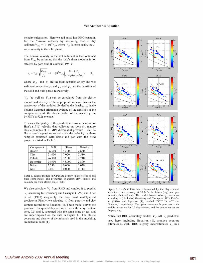
To check the quality of this prediction consider a subset ofHan’s (1986) velocity data collected on room-dry matureclastic samples at 30 MPa differential pressure. We useGassmann’s equations to calculate the velocity in thesesamples saturated with brine and gas with the fluidproperties listed in Table 1.

Component Bulk Shear DensityQuartz 36.600 45.000 2.650Clay 21.000 7.000 2.580Calcite 76.800 32.000 2.710Dolomite 94.900 45.000 2.870Brine 2.330 0.000 1.029Gas 0.017 0.000 0.112

Table 1. Elastic moduli (in GPa) and density (in g/cc) of rock andfluid components. The properties of quartz, clay, calcite, anddolomite are from Mavko et al. (1998).

We also calculate

€

Vp from RHG and employ it to predict

€

Vs according to Greenberg and Castagna (1992) and Kriefet al. (1990) (arguably the two most widely-usedpredictors). Finally, we calculate

€

Vs from porosity and claycontent according to Equation (1). These model curves areproduced for quartz/clay sediment with the clay contentzero, 0.5, and 1, saturated with the same brine or gas, andare superimposed on the data in Figure 1. The elasticconstants and density of the minerals used in this modelingare listed in Table (1).

Figure 1: Han’s (1986) data color-coded by the clay content.Velocity versus porosity at 30 MPa for brine- (top) and gas-saturated (bottom) rock. The model S-wave velocity curves areaccording to (clockwise) Greenberg and Castagna (1992), Krief etal. (1990), and Equation (1), labeled “GC,” “Krief,” and“Raymer,” respectively. The upper curves are for pure quartz, themiddle curves are for 0.5 clay content, and the bottom curves arefor pure clay.

Notice that RHG accurately models

€

Vp . All

€

Vs predictorsused here, including Equation (1), produce accurateestimates as well. RHG slightly underestimates

€

Vp in a



few pure-quartz samples and so do the

€

Vs predictors. Thepredictions are off-mark for one high-porosity samplewhich is unconsolidated and almost pure quartz Ottawasand (the dark-blue symbol of porosity 0.33). Nevertheless,we display this data point to further emphasize that neitherthe original RHG nor Equation (1) are suitable for softunconsolidated sediment.

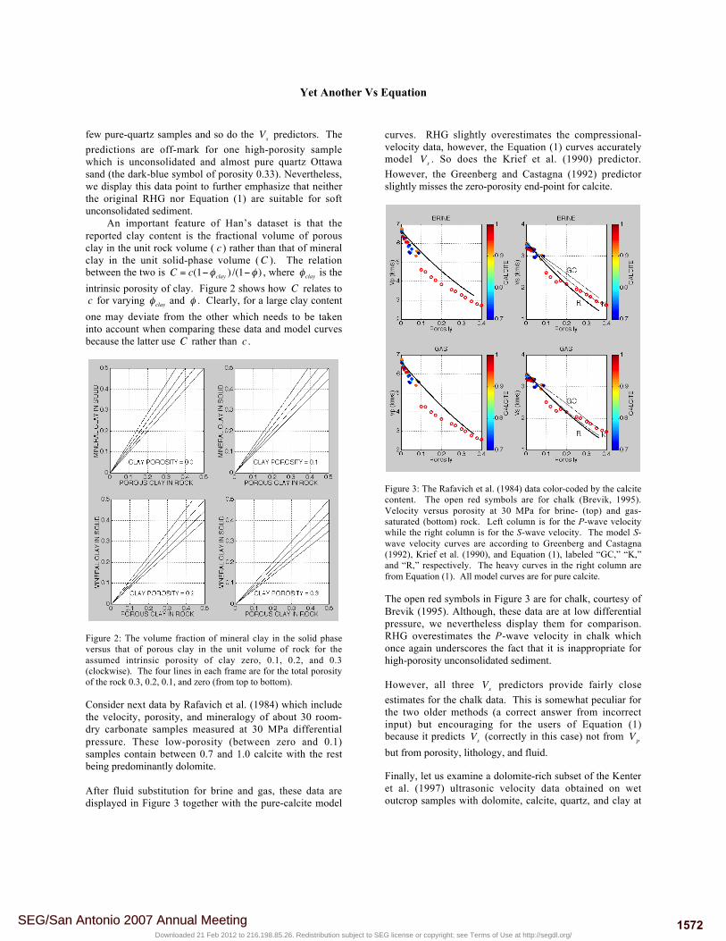
An important feature of Han’s dataset is that thereported clay content is the fractional volume of porousclay in the unit rock volume (

€

c ) rather than that of mineralclay in the unit solid-phase volume (

€

C ). The relationbetween the two is

€

C = c(1−φclay ) /(1−φ ) , where

€

φclay is theintrinsic porosity of clay. Figure 2 shows how

€

C relates to

€

c for varying

€

φclay and

€

φ . Clearly, for a large clay contentone may deviate from the other which needs to be takeninto account when comparing these data and model curvesbecause the latter use

€

C rather than

€

c .

Figure 2: The volume fraction of mineral clay in the solid phaseversus that of porous clay in the unit volume of rock for theassumed intrinsic porosity of clay zero, 0.1, 0.2, and 0.3(clockwise). The four lines in each frame are for the total porosityof the rock 0.3, 0.2, 0.1, and zero (from top to bottom).

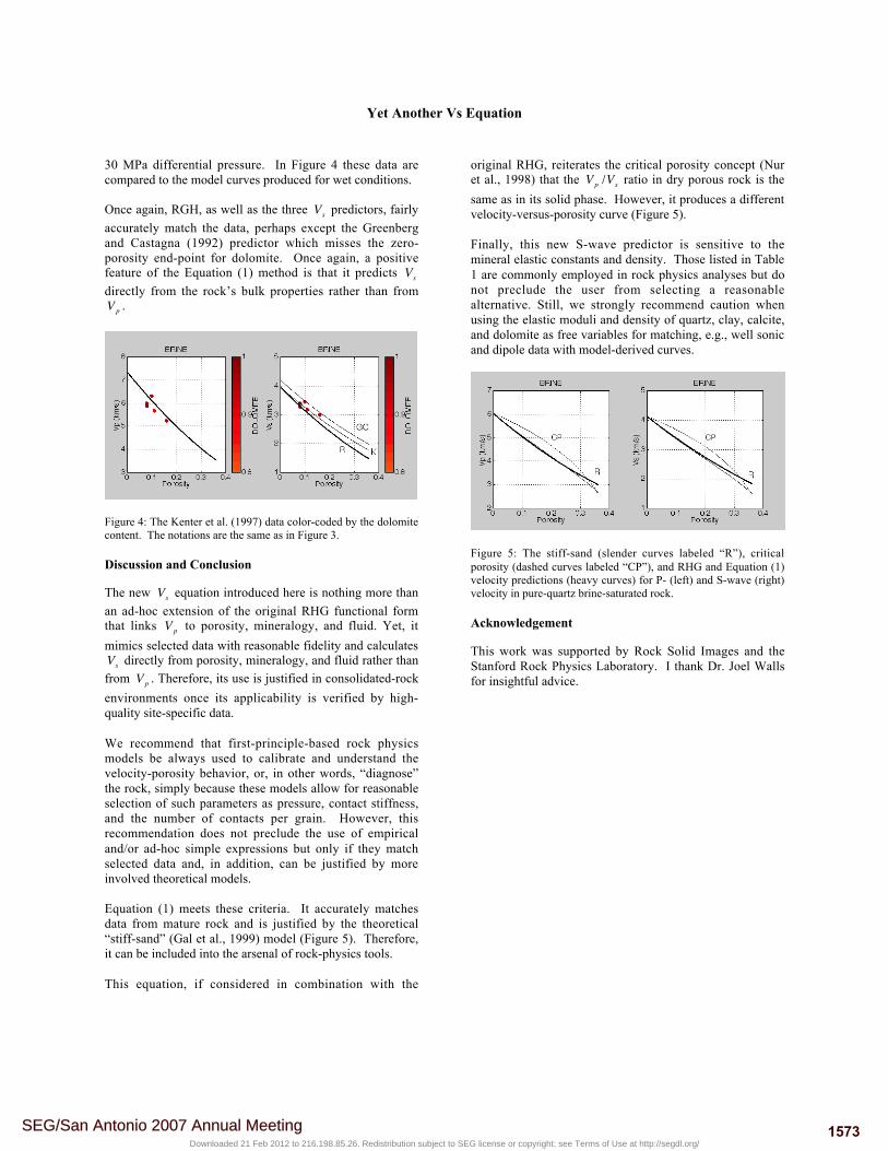
Consider next data by Rafavich et al. (1984) which includethe velocity, porosity, and mineralogy of about 30 room-dry carbonate samples measured at 30 MPa differentialpressure. These low-porosity (between zero and 0.1)samples contain between 0.7 and 1.0 calcite with the restbeing predominantly dolomite.

After fluid substitution for brine and gas, these data aredisplayed in Figure 3 together with the pure-calcite model

curves. RHG slightly overestimates the compressional-velocity data, however, the Equation (1) curves accuratelymodel

€

Vs . So does the Krief et al. (1990) predictor.However, the Greenberg and Castagna (1992) predictorslightly misses the zero-porosity end-point for calcite.

Figure 3: The Rafavich et al. (1984) data color-coded by the calcitecontent. The open red symbols are for chalk (Brevik, 1995).Velocity versus porosity at 30 MPa for brine- (top) and gas-saturated (bottom) rock. Left column is for the P-wave velocitywhile the right column is for the S-wave velocity. The model S-wave velocity curves are according to Greenberg and Castagna(1992), Krief et al. (1990), and Equation (1), labeled “GC,” “K,”and “R,” respectively. The heavy curves in the right column arefrom Equation (1). All model curves are for pure calcite.

The open red symbols in Figure 3 are for chalk, courtesy ofBrevik (1995). Although, these data are at low differentialpressure, we nevertheless display them for comparison.RHG overestimates the P-wave velocity in chalk whichonce again underscores the fact that it is inappropriate forhigh-porosity unconsolidated sediment.

However, all three

€

Vs predictors provide fairly closeestimates for the chalk data. This is somewhat peculiar forthe two older methods (a correct answer from incorrectinput) but encouraging for the users of Equation (1)because it predicts

€

Vs (correctly in this case) not from

€

Vp

but from porosity, lithology, and fluid.

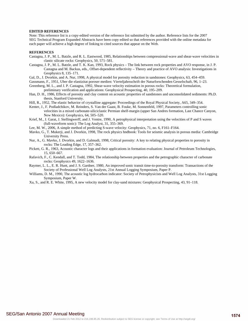
Finally, let us examine a dolomite-rich subset of the Kenteret al. (1997) ultrasonic velocity data obtained on wetoutcrop samples with dolomite, calcite, quartz, and clay at



30 MPa differential pressure. In Figure 4 these data arecompared to the model curves produced for wet conditions.

Once again, RGH, as well as the three

€

Vs predictors, fairlyaccurately match the data, perhaps except the Greenbergand Castagna (1992) predictor which misses the zero-porosity end-point for dolomite. Once again, a positivefeature of the Equation (1) method is that it predicts

€

Vs

directly from the rock’s bulk properties rather than from

€

Vp .

Figure 4: The Kenter et al. (1997) data color-coded by the dolomitecontent. The notations are the same as in Figure 3.

Discussion and Conclusion

The new

€

Vs equation introduced here is nothing more thanan ad-hoc extension of the original RHG functional formthat links

€

Vp to porosity, mineralogy, and fluid. Yet, itmimics selected data with reasonable fidelity and calculates

€

Vs directly from porosity, mineralogy, and fluid rather thanfrom

€

Vp . Therefore, its use is justified in consolidated-rockenvironments once its applicability is verified by high-quality site-specific data.

We recommend that first-principle-based rock physicsmodels be always used to calibrate and understand thevelocity-porosity behavior, or, in other words, “diagnose”the rock, simply because these models allow for reasonableselection of such parameters as pressure, contact stiffness,and the number of contacts per grain. However, thisrecommendation does not preclude the use of empiricaland/or ad-hoc simple expressions but only if they matchselected data and, in addition, can be justified by moreinvolved theoretical models.

Equation (1) meets these criteria. It accurately matchesdata from mature rock and is justified by the theoretical“stiff-sand” (Gal et al., 1999) model (Figure 5). Therefore,it can be included into the arsenal of rock-physics tools.

This equation, if considered in combination with the

original RHG, reiterates the critical porosity concept (Nuret al., 1998) that the

€

Vp /Vs ratio in dry porous rock is thesame as in its solid phase. However, it produces a differentvelocity-versus-porosity curve (Figure 5).

Finally, this new S-wave predictor is sensitive to themineral elastic constants and density. Those listed in Table1 are commonly employed in rock physics analyses but donot preclude the user from selecting a reasonablealternative. Still, we strongly recommend caution whenusing the elastic moduli and density of quartz, clay, calcite,and dolomite as free variables for matching, e.g., well sonicand dipole data with model-derived curves.

Figure 5: The stiff-sand (slender curves labeled “R”), criticalporosity (dashed curves labeled “CP”), and RHG and Equation (1)velocity predictions (heavy curves) for P- (left) and S-wave (right)velocity in pure-quartz brine-saturated rock.

Acknowledgement

This work was supported by Rock Solid Images and theStanford Rock Physics Laboratory. I thank Dr. Joel Wallsfor insightful advice.


EDITED REFERENCES Note: This reference list is a copy-edited version of the reference list submitted by the author. Reference lists for the 2007 SEG Technical Program Expanded Abstracts have been copy edited so that references provided with the online metadata for each paper will achieve a high degree of linking to cited sources that appear on the Web. REFERENCES Castagna, J. P., M. L. Batzle, and R. L. Eastwood, 1985, Relationships between compressional-wave and shear-wave velocities in

clastic silicate rocks: Geophysics, 50, 571–581. Castagna, J. P., M. L. Batzle, and T. K. Kan, 1993, Rock physics – The link between rock properties and AVO response, in J. P.

Castagna and M. Backus, eds., Offset-dependent reflectivity – Theory and practice of AVO analysis: Investigations in Geophysics 8, 135–171.

Gal, D., J. Dvorkin, and A. Nur, 1998, A physical model for porosity reduction in sandstones: Geophysics, 63, 454–459. Gassmann, F., 1951, Uber die elastizitat poroser medien: Vierteljahrsschrift der Naturforschenden Gesselschaft, 96, 1–23. Greenberg, M. L., and J. P. Castagna, 1992, Shear-wave velocity estimation in porous rocks: Theoretical formulation,

preliminary verification and applications: Geophysical Prospecting, 40, 195–209. Han, D. H., 1986, Effects of porosity and clay content on acoustic properties of sandstones and unconsolidated sediments: Ph.D.

thesis, Stanford University. Hill, R., 1952, The elastic behavior of crystalline aggregate: Proceedings of the Royal Physical Society, A65, 349–354. Kenter, J., F. Podladchikov, M. Reinders, S. Van der Gaast, B. Fouke, M. Sonnenfeld, 1997, Parameters controlling sonic

velocities in a mixed carbonate-siliciclastic Permian shelf-margin (upper San Andres formation, Last Chance Canyon, New Mexico): Geophysics, 64, 505–520.

Krief, M., J. Garat, J. Stellingwerff, and J. Ventre, 1990, A petrophysical interpretation using the velocities of P and S waves (full-waveform sonic): The Log Analyst, 31, 355–369.

Lee, M. W., 2006, A simple method of predicting S-wave velocity: Geophysics, 71, no. 6, F161–F164. Mavko, G., T. Mukerji, and J. Dvorkin, 1998, The rock physics hndbook: Tools for seismic analysis in porous media: Cambridge

University Press. Nur, A., G. Mavko, J. Dvorkin, and D. Galmudi, 1998, Critical porosity: A key to relating physical properties to porosity in

rocks: The Leading Edge, 17, 357–362. Pickett, G. R., 1963, Acoustic character logs and their applications in formation evaluation: Journal of Petroleum Technologies,

15, 650–667. Rafavich, F., C. Kendall, and T. Todd, 1984, The relationship between properties and the petrographic character of carbonate

rocks: Geophysics 49, 1622–1636. Raymer, L. L., E. R. Hunt, and J. S. Gardner, 1980, An improved sonic transit time-to-porosity transform: Transactions of the

Society of Professional Well Log Analysts, 21st Annual Logging Symposium, Paper P. Williams, D. M., 1990, The acoustic log hydrocarbon indicator: Society of Petrophysicists and Well Log Analysts, 31st Logging

Symposium, Paper W. Xu, S., and R. E. White, 1995, A new velocity model for clay-sand mixtures: Geophysical Prospecting, 43, 91–118.


yet another vs equation - rock solid images · yet another vs equation jack dvorkin*, stanford...

Documents