1

Yes, One-day International Cricket ‘In-play’ Trading Strategies can be

Profitable!

Abstract

In this study, we employ a Monte Carlo simulation technique for estimating the conditional

probability of victory at any stage in the first or second innings of a one-day international (ODI)

cricket match. This model is then used to test market efficiency in the Betfair ‘in-play’ market

for large sample of ODI matches. We find strong evidence of overreaction in the first innings.

A trading strategy of betting on the batting team after the fall of a wicket produces a significant

profit of 20%. We also find some evidence of underreaction in the second innings although it

is less economically and statistically significant than the first innings overreaction. We also

implement trades when the discrepancy between the probability of victory implied by current

market odds differs substantially from the odds estimated by our Monte Carlo simulation

model. We document a number of trading strategies that yield large statistically significant

positive returns in both the first and second innings.

Keywords: in-play betting markets; Trading strategies; ODI Cricket; web-scraping; Monte

Carlo simulation

2

1. Introduction

According to Thaler and Ziemba (1988), betting markets provide an ideal setting in which to

test market efficiency. Betting markets have a key advantage over stock exchanges – the

uncertainty surrounding the outcome of a sporting wager is definitively resolved at a well-

defined termination point. The key difficulty in testing the efficiency of stock markets is that

the “true” price of the stock is never revealed, meaning that efficiency is generally tested as

part of a joint hypothesis with rational expectations or a particular asset pricing model. This

problem does not arise in sports betting markets, where the outcome is revealed at the

completion of the match/game.

Moreover, it is possible to examine sports betting markets for the same types of

systematic effects that have been documented in stock markets. For example, various authors

have documented an overreaction in stock prices to certain announcements of important news.

In the context of sports betting, one can examine how the “in-play” odds react to important

events (e.g., the loss of a wicket in a cricket match or the scoring of a goal in a football match).

Similarly, in stock markets semi-strong form efficiency can be tested by considering

whether publicly available information can be processed in a way that leads to exploitable

trading opportunities. However, one can never be sure that the risk of the trading strategy was

accurately quantified. A cleaner test is available in sports betting markets whereby publicly

available information can be used to construct a betting rule, and the outcome of each bet is

revealed with certainty at the end of each game. That is, the odds available on a sporting bet

provide an unambiguous estimate of the market’s perceived probability of an event occurring.

If the market systematically misestimates these probabilities, then profitable trading strategies

can be constructed.

3

To this end, we analyse the efficiency of the Betfair1 ‘in-play’ market relating to one-

day international cricket (ODI). Specifically, we examine the efficiency of the market reaction

to significant value-relevant events (specifically, the fall of a wicket), via the execution of a

trading rule based on a comprehensive linear programming model that uses publicly available

information. We find some evidence of systematic inefficiencies that are closely analogous to

similar effects that have been documented in stock markets.

ODI cricket is a “bat and ball” sport in which one team bats and sets a total score in the

first innings, and the opposing team then takes its turn to bat and “chases” the set score in the

second innings. The main cricket playing nations are Australia, New Zealand, England, South

Africa, India, Pakistan, Sri Lanka, Bangladesh and the West Indies. Each team would play an

average of approximately 20 ODIs per year. A major World Cup is held every four years.

Readers unfamiliar with the game of cricket are directed to Section A.1 of the appendix, which

summarises the rules that are central to our paper.

There are a number of potential factors that influence a ODI cricket team’s expected

score. The more resources a team has available, the more runs they are likely to score

throughout the remainder of the innings. The value of each of these resources on a team’s

expected score is dependent on the amount of the other resources available.2 In this sense, any

attempt to model or predict the outcome of a cricket innings must account for the interaction

between the available resources.

We develop a more sophisticated and more accurate approach to modelling these

interactions than achieved in the previous literature. In particular, we develop a comprehensive

1 Betfair is an on-line betting exchange on which bettors are able to post “back” and “lay” odds in precisely the

same way that traders place “bid” and “ask” quotes when trading stocks. In-play betting occurs when bettors are

able to trade during the course of the game, as it evolves. Anyone with a (free) Betfair account and access to the

Internet can place a bet. However, in private communications, Betfair have advised that customers in the

following countries are blocked from betting on their exchange: the US, China, France, Hong Kong, Japan,

Singapore, South Africa and Turkey. Betfair retains a 5% commission on winning bets. 2 For example, having six wickets remaining in the very last over of a team’s innings is of little benefit in aiding

its push towards victory. Similarly, having 20 overs remaining (i.e. 40% of the maximum batting time) is of little

benefit to a team that has already lost nine wickets.

4

dynamic programming model that models the ball-by-ball evolution of the match through to its

conclusion. We implement this model using a Monte Carlo simulation approach that tracks

the ball-by-ball evolution of the match through to its conclusion, via many simulations; an

approach that provides the basis for a number of tests of statistical significance. Notably, our

study is the first to test the efficiency of the ‘in-play’ market with a model that accounts for

differences in team skill and the first to use ball-by-ball data. Accordingly, our model should

have a much higher likelihood of identifying any market inefficiency and any exploitable

mispricing.

Brooker and Hogan (2011) create a model that includes variables for match conditions

and run rate required (based on a large sample of 310 games), but their model is restricted to

the second innings only.3 Importantly, our model can estimate the probability of victory at any

point throughout either innings of a cricket match. Further, we partition the innings into

multiple segments and separately estimate the model coefficients for each, thereby capturing

non-linearities in the data. Compared to Brooker and Hogan (2011), we condition on four

additional variables – current run rate, current batter score and the career batting averages and

strike rates of all 22 players in the match – which we argue will improve the predictive ability

of the model. Because of the additional complexity associated with accounting for each

individual player, our method is based on Monte Carlo simulation. Finally, we have a very

large sample comprising 1,101 ODI matches and utilise highly granular ball-by-ball data.

There are considerable benefits of testing efficiency in an ‘in-play’ market compared

with traditional studies of pre-match odds or financial markets. In particular, ‘in-play’ sports

betting markets are not affected by the problem of private information because once a match

has begun, any new information about the state of the game is instantly observed by all. As

3 That is, they model only the probability of the second team winning, conditional on the score set by the team

that batted first.

5

such, we would expect changes in the odds to accurately and speedily reflect the market’s

interpretation of the information arrival.

Our out-of-sample dataset contains ball-by-ball scores and odds for 186 ODI matches,

producing a total of 101,176 ‘news-events’ which represent the outcome of every ball that is

bowled in the game. Having detail at a ball-by-ball level means that we are able to place

hypothetical wagers immediately after any ball is bowled as opposed to being restricted to

betting at the conclusion of any given over. Our model also includes several variables that aim

to capture the ability of each individual player.

Our key findings can be summarised as follows. We find strong evidence of

overreaction in the first innings. A trading strategy of betting on the batting team after the fall

of a wicket under strict trading restriction results in a profit of 20.8% that is significant at the

1% level. We also find some evidence of underreaction in the second innings although it is

less economically and statistically significant than the first innings overreaction. We also

implement trades when the discrepancy between the probability of victory implied by current

market odds differs substantially from the odds estimated by our Monte Carlo simulation

model. We document a number of trading strategies that yield large statistically significant

positive returns in both the first and second innings.

The remainder of this paper organised as follows. In Section 2, we present a brief

background and literature review. Section 3 then outlines the research method, while the results

are presented and discussed in Section 4. Section 5 concludes.

2. Background and Literature Review

2.1 Cricket Literature

Clarke (1988) is one of the first attempts at modelling a team’s total score with a dynamic

programming model. Simple in nature, it is based on the idea that the average run rate targeted

by a team is inversely related to the probability of getting out. Duckworth and Lewis (1998)

6

developed a model for forecasting expected runs based on a two-factor relationship between

wickets in hand and overs remaining. Bailey and Clarke (2006) use a multiple linear regression

model that incorporates variables such as experience, quality, form and home advantage.

Unlike Duckworth and Lewis (1998), this model only predicts the expected total score from

the start of the innings. Once the innings has begun, they adjust their predicted score based on

the quantity of resources used according to the Duckworth and Lewis (1998) tables.4

Swartz, Gill and Muthukumarana (2009) develop a model for predicting potential

outcomes for each delivery. They use a single latent variable for determining both the runs and

wickets process which assumes that the expected run rate is inversely related to the probability

of a wicket. Their model does not provide a good empirical fit to the data, particularly in the

later stages of an innings. Brooker and Hogan (2011) use Bayes’ rule to estimate the impact

of ground conditions on the distribution of first innings scores.

2.2 Efficiency of Sports Betting Markets

One of the most frequently analysed sports betting markets is horse racing. The general

consensus is that the racetrack market is very efficient – probabilities implied by the market

odds match very closely to the true probabilities. However, several anomalies have been

uncovered. For example, one of the earliest documented is that punters systematically

underestimate the chances of short-odds horses and overvalue those of long odds horses – the

so-called, ‘favourite-longshot’ bias (Griffith, 1949; McGlothlin, 1956; Ali, 1977; Weitzman,

1965; Snyder, 1978; Asch, Malkiel and Quandt, 1982; Ziemba and Hausch, 1987).

The structure of the horse racing market differs from the cricket betting market in three

key ways. First, relatively high commissions are charged by the racetracks – for example,

4 Clarke (1988) also develops a dynamic programming model to determine the optimal scoring rate. His analysis

suggests that a good strategy is to score quickly at the beginning of the innings and slow down if wickets are lost.

A number of papers since then have used similar dynamic programming models (Johnston, Clarke and Noble,

1993; Preston and Thomas, 2000; Norman and Clarke, 2007, 2010; Brooker, 2009) and analysed optimal strategy

(Preston and Thomas, 2000). Other aspects of cricket strategy that have been studied include the analysis of the

optimal batting order to maximise expected runs (e.g. Ovens and Bukiet, 2006; Norman and Clarke, 2007, 2010)

The general conclusion is that adjusting the batting order to suit the match conditions results in an increase in the

probability of winning (on average).

7

Asch, Malkiel and Quandt (1982) report a commission of 18.5%. In our study, commissions

are much less influential since the maximum charged by Betfair is 5%, paid on winning bets

only. Second, anecdotal evidence about racetrack bettors being more concerned with having a

fun day out at the track as opposed to being strictly rational expected utility maximisers, is

much less likely to apply to our setting.5 We argue this because of the online nature of the

exchange in which the majority of bets are placed by people who are not actually at the game.

Third, for horse-racing there is no in-play market – all bets must be placed before the beginning

of the race. Moreover, horse racing also involves more relevant information at the venue (e.g.,

the condition of the track and other horses) making on-line betting relatively less attractive.

Tests of market efficiency and investor rationality have been conducted in many

professional sports betting markets around the world. The spreads betting market in the

National Football league (NFL) in the US has been shown to exhibit several biases. For

example, Golec and Tamarkin (1991) find that the market underestimates the home team

advantage and has a bias against underdogs. However, these biases have been shown to have

diminished over time (Gray and Gray, 1997). Dare and Holland (2004) believe that previous

models suffer from collinearity problems because the home team is twice as likely to be the

favourite and these variables are therefore not independent as the model assumes. Using a new

specification that corrects for this bias, they report the renewal of a bias favouring bets on home

underdogs.6

In short, the message we gain from this brief coverage of the sports betting literature is

that efficiency anomalies of various types, have been identified across a wide range of sports

betting markets. As we will see in the next section, in a more limited way this is also true of

5 Indeed, the horse-racing favourite/longshot bias has been explained in terms of “bragging rights” associated with

backing a longshot winner. 6 The betting markets of many other international sports have been used for testing market efficiency including

golf (Docherty and Easton, 2012); soccer (Demir, Danis and Rigoni, 2012); tennis (Forest and McHale, 2007);

Australian Rugby League and Australian Football League (Brailsford, Gray, Easton and Gray, 1995) and Major

League Baseball (Paul and Weinbach, 2008).

8

the cricket betting markets and, thus, we argue that much more extensive and powerful testing

is possible than is currently achieved in existing studies. Our paper steps up to provide such an

extension to this literature.

2.3 Cricket Betting Markets

There is a large volume of money wagered on most ODIs relative to other sports. For example,

Ryall and Bedford (2010) report that the average amount of money bet ‘in-play’ on Betfair for

an Australian Football League (AFL) match is $80,000, while blockbuster games such as the

grand final can attract up to $140,000. Notably, for the 186 out-of-sample ODIs in our study

the average amount bet was over $8 million, with some games drawing in excess of $20 million.

One reason for the higher betting volumes in ODI cricket games is that cricket is viewed by an

international audience, particularly in India where ODI matches are broadcast on cable TV

channels. Also, ODI cricket matches are played out over a period of 8-9 hours and, thus, often

involve considerable swings in the relative position of the two teams, making them ideal

candidates for in-play betting. Moreover, for almost every ODI, instant updates on the position

of the game are available on-line and via mobile devices.

Bailey (2005) is the first study to look for inefficiencies in the cricket betting market,

analysing “head-to-head” match-ups in the 2003 World Cup. A head-to-head match-up is an

exotic bet where bettors have to predict which of two players they think will score more runs

in the match. Bailey’s (2005) models take into account many factors: batting position,

experience, home country advantage, match time, innings sequence, opposition, performance,

and form. The most successful of the models achieved an ROI of 35%, suggesting that the

head-to-head market may be inefficient. Notably, the head-to-head market is a pre-match

market – that is, bets are not made once the game has commenced – and so is not directly

comparable to the ‘in-play’ analysis of our study.

Using a ball-by-ball dataset of market odds for 15 ODI cricket matches, Easton and

Uylangco (2006) analyse the changes in odds in response to the outcome of each ball bowled.

9

From our perspective, their most interesting finding is the association between the outcome of

a particular ball and the payoffs of the six preceding balls. They suggest that this is evidence

that the market has some ability to predict the outcome of future deliveries. Overall this study

is more of a description of how the in-play prices react to certain outcomes as opposed to a

definitive test of market efficiency. Absent a model for the probability of victory, they are

silent on the question of mispricing.

2.4 In-Play Betfair Market

In-play markets, like Betfair, allow customers to bet on the outcome of a sporting event while

it is in progress as opposed to a traditional market where bets can only be placed prior to the

game commencing. Betfair operates in a similar way to a stock exchange. Opposing bets are

matched anonymously by Betfair with a commission being charged on the winning bet (see the

Appendix).7 The advantage of the stock exchange style business model from Betfair’s

perspective is that they are not exposed to any risk with regard to the outcome of the games as

would be a traditional bookmaker. They allow punters to decide how much they are willing to

bet and at what odds.8

The Betfair interface shows users the odds that are currently available to ‘back’ or lay’

each team as well as the market depth for each selection (see Figure A1 in the Appendix). To

illustrate the difference between a ‘back’ and ‘lay’ wager we provide, in Figure A2 of the

Appendix an example of the payoffs to a variety of bets placed using the odds shown in Figure

A1. A lay bet is analogous to short selling in the stock market. If a punter wants to bet on a

particular team winning the game they can either place a back bet on that team or lay odds for

the opposition.9

7 We assume for the purposes of our study that we have no Betfair points and thus pay the full commission rate. 8 A traditional bookmaker determines the odds at which punters can bet and they adjust the odds in an attempt to

‘balance their book’ which essentially involves having an even amount of money at stake on each result to ensure

that they make a profit. 9 If a punter places a $100 lay bet on a particular team, they receive the $100 stake upfront but must pay an amount

equal to $100 multiplied by the agreed odds if that team wins. So the potential loss can be greater than the original

$100 stake.

10

Three key existing papers test the efficiency of in-play betting markets and they all use

Betfair data. Ryall and Bedford (2010) analyse the in-play market for the 2009 AFL season,

Docherty and Easton (2012) analyse the 2008 Ryder Cup Golf Tournament, while Brown

(2012) analyses the 2008 Wimbledon final between Roger Federer and Rafael Nadal.

2.5 Our Contribution

In the context of the preceding review of the key relevant work, we make a number of

contributions to the existing literature. First, we construct a detailed dynamic programming

model to forecast (a) the total score of the batting team during the first innings of the match,

and (b) the probability that the chasing team will win the match. Previous research has, at

most, considered the probability of a chasing team victory, conditional on the target score

already set by the first-batting team. Our model also conditions on the score of the current “not

out” batsmen (e.g., it is less likely that a batsman will be dismissed if they have already

compiled a substantial score than if they are just beginning their own innings).

Another key difference between our model and the previous models is that we partition

each innings into various segments based on the number of overs and wickets remaining and

we estimate model parameters separately for each of the segments. We show that this

conditioning approach produces more accurate predictions, since the relative importance of

both wickets and overs remaining depend on the match situation. In summary, our first

contribution is a more detailed and accurate dynamic programming model. We implement this

model using a Monte Carlo simulation approach that tracks the ball-by-ball evolution of the

match through to its conclusion, over many simulations. This approach provides the basis for

a number of tests of statistical significance.

Our second contribution is the application of our model to a large sample of in-play

exchange betting markets. No prior studies have analysed the rich and deep in-play exchange

betting data for ODI cricket matches. Moreover, we develop a number of tests of efficiency.

In particular, we examine the possibility of overreaction and momentum effects, as have been

11

documented in other financial markets. Finally, we introduce a number of methodological

innovations that are likely to be of use in future research. For example, we develop techniques

for (a) synchronising odds and game score data from separate data feeds, and (b) calibrating

model estimates to account for cases where one of the teams is a strong pre-game favourite.

3. Research Design

3.1 Hypotheses

We test the betting markets version of weak-form efficiency suggested by Thaler and Ziemba

(1988), namely, that ‘no bets should have positive expected values’ as opposed to the strong

form which says that ‘all bets should have negative expected profits equal to the amount of

commission’. De Bondt and Thaler (1985) document empirical evidence of overreaction to

recent news in stock price data. They find that stocks that have extreme price movements in

one direction tend to be followed by subsequent price movements in the opposite direction. In

a similar fashion, we seek to test for evidence of overreaction in a sports betting market. This

leads to our first hypothesis:

H1: Overreaction Hypothesis The Betfair ‘in-play’ market overreacts to the outcome

of certain (“high news”) ODI balls in a systematic way.

We also examine the market for evidence of momentum effects similar to those found in stock

price returns (Jegadeesh and Titman, 1993):10

H2: Underreaction Hypothesis: The Betfair ‘in-play’ market underreacts to the outcome

of certain (“high news”) ODI balls in a systematic way.

Hypotheses 1 and 2 look for “irrational” behaviour of the market around significant

ODI ‘news’ events. We also test if the market systematically misevaluates the current state of

the match independent of any under or overreaction to recent events. We do this by comparing

10 In stock markets, there tends to be consistent evidence of reversals – both at the short-term end (less than four

weeks) and longer-term (12-36 months) and of momentum over the intermediate term straddled by these two

(maximising at about the six-month horizon).

12

the probability of victory determined by our model, with the probability of victory implied by

the market odds; executing a trading strategy when the discrepancy between the two models

crosses a certain threshold.

H3: Mis-estimated Probability of Victory Hypothesis: The Betfair ‘in-play’ market

systematically misestimates the probability of victory during an ODI cricket

match.

3.2 Data

Several extensive datasets are created and merged in this study. The first dataset contains ball-

by-ball information for 1,101 one-day internationals from June 2001 to March 2013, excluding

all games between non-test playing nations and any games shortened due to rain or other

interruptions.11 In total there are 601,744 balls recorded, each containing the following

information: the over number; the ball number; the number of runs scored; the number of

extras; whether the batsman was out; the batsman’s name; the bowler’s name; the match

number; the innings number; the date; and the required run rate (for second innings only). Table

1 shows the frequency of each ball outcome in our sample. We obtain these unique data by

executing a web-scraping program in Python.12 This program reads the ball-by-ball text

commentaries available on Cricinfo,13 and extracts the relevant information.

We also obtain data from Fracsoft, a company that records live prices offered by

Betfair. This sample covers 186 one-day internationals played from June 2006 to September

2012. Notably, these odds data are available after every ball, rather than only after every over

as in previous studies. Although the Betfair dataset contains a time stamp, it does not contain

the current score in the cricket match at that time. Perversely, although the ball-by-ball Cricinfo

dataset described above contains the scores it does not have a timestamp. Moreover, to the best

11 Since test playing nations comprise the best teams in world cricket, games involving non-test playing nations

tend to be very one-sided. Accordingly, other things being equal, such one-sided games are less attractive to

potential bettors. 12 Python is a widely used general-purpose, high-level programming language (see www.python.org). 13 Cricinfo (www.espncricinfo.com) is the world’s leading cricket website and in the top five single-sport websites

in the world. Its content includes live news and ball-by-ball coverage of all Test and one-day international matches.

13

of our knowledge this combined timestamp/score information is not publicly available in any

form. Accordingly, we obtain a third dataset from Opta, another sports data provider

containing the timestamp for every ball that was bowled for each of the 186 matches for which

we have the live odds data. Thus, exploiting all three data sources (Cricinfo, Fracsoft and Opta)

we match up each ball with the corresponding live odds that were available at that time. We

also require the career batting average and strike rate of every player in every match in our

sample, as well as the batting order for each game. Again we extract this information from

Cricinfo using the Python web-scraping algorithm.

It is well established that testing a model against the same data that was used to estimate

the parameters will result in over-fitting. Accordingly, the 186 matches for which we have live

odds information from the original ball-by ball dataset are quarantined as the out-of-sample

dataset for testing our trading rules. All other games in the ball-by-ball dataset constitute the

“in-sample” component for estimating the model parameters.

14

3.3 Modelling

3.3.1 Core Features of the Dynamic Programing Model

Dynamic programming models applied to cricket, take on board all the available conditioning

information to produce a probability for every possible outcome of the next ball bowled. Such

models used by Carter and Guthrie (2004) only condition on balls remaining and wickets in

hand, while Brooker and Hogan (2011) also add in the run rate required and a conditions

variable. Our model extends the dynamic program in several key ways from the previous

literature. First, previous work only models the probability of victory for the second innings

(conditioned on the score having been set by the first batting team), whereas our model

considers ball-by-ball at any time in the ODI. Second, we allow the probability of a batsman

getting out or scoring a particular number of runs to vary as a function of their own current

score. It is a widely held belief among cricket experts and fans that a batsman takes time to get

their ‘eye-in’ and their performance generally improves the longer they have been batting.14

Another key difference between our model and the previous models is that we split each

innings up into various segments based on the number of overs and wickets remaining and we

estimate model parameters separately for each of the segments. This allows the intercepts and

slope coefficients to vary throughout the innings in a non-linear way. We argue that this

conditioning approach produces more accurate predictions, since the relative importance of

both wickets and overs remaining depend on the match situation.15

We develop separate models for the first and second innings. For the first innings we

allow the outcome of any particular delivery to be influenced by six factors: (1) Balls (b) –

number of balls remaining in the innings; (2) Wickets (w)– number of wickets remaining for

the batting team; (3) Run Rate (RR) – current run rate per over of the batting team achieved in

14 We do not include the conditions variable used by Brooker and Hogan (2011) because it uses the result of the

match to adjust the distribution of second innings scores. 15 For example, the difference between being 3/250 or 6/250 off 45 overs is not the same as the difference between

being 3/100 or 6/100 after 20 overs.

15

the innings to date; (4) Score (s) – current score of the batsman on strike; (5) Average (a) –

career batting average of the batsman on strike; and (6) Strike Rate SR (k) – career strike rate

of the batsman on strike.16

It is important to note that the combination of our dynamic programming model and

Monte Carlo simulation approach means that complexity and computing time increases

exponentially with each additional variable. Consequently, our approach is to expand on the

previous literature by including a carefully chosen subset of variables that we consider are most

likely to have the greatest explanatory power. Specifically, these included variables relate to

the current score of the “not out” batsman (because there is strong evidence that a batsman who

is “set” is more likely to score more runs and less likely to lose his wicket) and the quality of

the batsman (based on his batting average and batting strike rate).

While we also considered counterpart variables relating to bowlers, we deemed them

to be less important (and, hence expendable) since each bowler is limited to just 10 overs per

ODI. Moreover, ignoring the bowling-related variables is broadly supported by the widely-

held belief that ODI cricket is a “batsmen’s game” (e.g., see Dasgupta, 2013).17 We also

rejected the inclusion of information about the circumstances of the game – for example,

whether one of the teams was playing at a favoured home ground or whether the game was a

final or a less important qualification game. While these variables are also likely to be relevant

initially, their informativeness, relative to the observed score, is likely to decline as the match

progresses.

16 Importantly, we use the career statistics of each batsman up until the start of the game in question to ensure that

we are not conditioning on information that occurred subsequently to the game being modelled. 17 Indeed, there is a fundamental asymmetry in ODI cricket. While an individual batsman is allowed to bat for the

entire 50 overs allotted to his team with no limit on his score, no one bowler can bowl more than 20% of the total

overs available in any given ODI innings. Thus, an individual batsman is more likely to have a greater impact on

the game than is any single bowler. For example, only 2 of the top 40 ODI man-of-the match winners are

predominately bowlers – Shaun Pollock and Wasim Akram. See

http://stats.espncricinfo.com/ci/content/records/283705.html (accessed 9 July 2015).

16

For each ball bowled, one of three general outcomes are possible: (1) a wide or no-ball

(i.e., an illegal delivery) with probability E; (2) if the ball is not a wide or no-ball then a wicket

will fall with probability 𝑂(𝑏, 𝑤, 𝑅𝑅, 𝑠, 𝑎, 𝑘); or (3) if the ball is not a wide or no-ball and a

wicket has not fallen, the batsman scores 𝑥 runs with probability 𝑃(𝑥; 𝑏, 𝑤, 𝑅𝑅, 𝑠, 𝑎, 𝑘),

where 𝑥 𝜖 {0,1, … 6}.18 For modelling expediency, we assume that (a) each of these outcomes

are mutually exclusive; (b) only one run is scored when a wide or no-ball is bowled; and (c)

byes and leg byes are runs scored by the batsman.19

We wish to estimate 𝐷(𝑟; 𝑏, 𝑤, 𝑅𝑅, 𝑠1, 𝑠2, 𝑓, 𝑝1, 𝑝2, 𝐴, 𝐾) which represents the

probability of scoring 𝑟 or fewer runs from the remaining 𝑏 deliveries, with 𝑤 wickets in hand,

a current run rate of 𝑅𝑅, batsman one on a score of 𝑠1, batsman two on a score of 𝑠2, a dummy

variable 𝑓 equal to 1 if batsman one is facing, p1 (p2) batting position of batsman one (two),

career average A and strike rate K of every player in the team. Accordingly, the distribution

function for the first innings is described by the following equation:

𝐷(𝑟; 𝑏, 𝑤, 𝑅𝑅, 𝑠1, 𝑠2, 𝑓, 𝑝1, 𝑝2, 𝐴, 𝐾) =

𝐸 × 𝐷(𝑟 − 1; 𝑏, 𝑤, 𝑅𝑅∗, 𝑠1, 𝑠2, 𝑓, 𝑝1, 𝑝2, 𝐴, 𝐾)

+ (1 − 𝐸) ∙ 𝑂(𝑏, 𝑤, 𝑓 ∙ 𝑠1 + (1 − 𝑓) ∙ 𝑠2, 𝑎∗/𝑘∗)

× 𝐷(𝑟; 𝑏 − 1, 𝑤 − 1, 𝑅𝑅∗, 𝑠1 − 𝑓 ∙ 𝑠1, 𝑠2 − (1 − 𝑓) ∙ 𝑠2, 𝑓∗, 𝑝1∗, 𝑝2∗, 𝐴, 𝐾)

+ (1 − 𝐸) (1 − 𝑂(𝑏, 𝑤, 𝑓 ∙ 𝑠1 + (1 − 𝑓) ∙ 𝑠2, 𝑎∗/𝑘∗))

× ∑ 𝑃(𝑥; 𝑏, 𝑤, 𝑅𝑅∗, 𝑓 ∙ 𝑠1 + (1 − 𝑓) ∙ 𝑠2, 𝑘∗)

𝑖𝜖(0,1,..6)

× 𝐷(𝑟 − 𝑥; 𝑏 − 1, 𝑤, 𝑅𝑅∗, 𝑠1 + 𝑓 ∙ 𝑥, 𝑠2 + (1 − 𝑓) ∙ 𝑥, 𝑓∗, 𝑝1, 𝑝2, 𝐴, 𝐾) (1)

18 While it is possible seven runs can be scored if the batsman hits a six off a no-ball, to keep our modelling more

manageable, this highly unusual event is excluded. 19 Since these events they happen so infrequently, our simplifications have minimal impact on the estimation

procedure while greatly simplifying the modelling process.

17

where 𝐴 and 𝐾 are 11 × 1 vectors containing the career average and strike rate, respectively,

of each player in the team, 𝑎∗ = career average of the batsman on strike, 𝑘∗ = career strike rate

of the batsman on strike and the remaining variables are as defined above.

For notational convenience, 𝑅𝑅∗ denotes the new run rate after scoring 𝑖 runs off the

given ball and 𝑓∗ denotes the updated value for 𝑓 which will change to (1 − 𝑓) if the batsman

scores an even number of runs on the last ball of the over or an odd number of runs on any

other ball. The model for the second innings is essentially the same except that we use the run

rate required for victory, RRR, instead of the run rate achieved in the innings to date. The other

main difference will be that the distribution will be capped at the target score, given victory

defined by the rules of cricket.20

3.3.2 Probability of Losing a Wicket

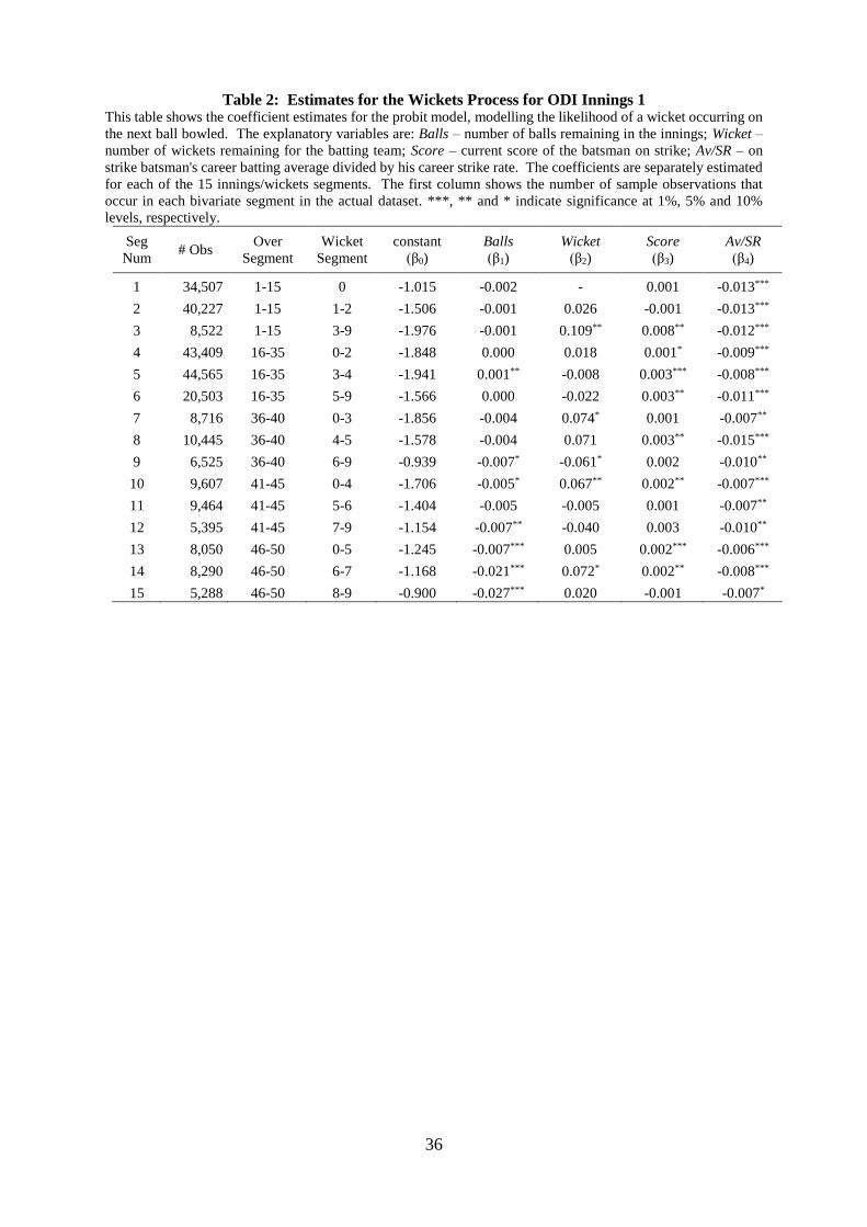
We estimate the probability of losing a wicket on a given ball using a probit model, as a

function of Balls, Wickets, Score, and Av/SR. To illustrate, the results of running the regression

for each of the 15 first innings segments is displayed in Table 2.21 The table shows that the

estimated coefficients on balls remaining are not significant for seven out of the first eight

innings segments but are significantly negative for all but one of the last seven segments. The

negative signs are consistent with the idea that the more balls that are remaining in the innings,

the higher the cost of losing a wicket because the batting team runs the risk of not using up all

of their available overs. In the latter stages of the innings however, the cost of losing a wicket

is lower because the potential number of overs wasted is much smaller and so teams take a

more aggressive approach and, therefore, the likelihood of a wicket falling is higher.

20 For the purposes of estimating the probability of a wide or no ball, we assume that the chances of the bowler

conceding a wide or no-ball is identical for all match situations and is independent of the conditioning variables

used for the wickets and run scoring processes. The results are not sensitive to this assumption given the relatively

low frequency of these events. 21 To conserve space, we do not tabulate the second innings counterpart – details are available from the authors

upon request.

18

Only five out of the 15 coefficients on wickets remaining are significant, but this does

not mean that wickets remaining is unimportant factor in determining the likelihood of a wicket

falling. This is because we have split the sample up into different segments based on the

number of wickets in hand and so, by construction, we have reduced the variation in the wickets

remaining variable, which naturally decreases the likelihood of finding significant coefficients.

Eight of 15 cases show a significant coefficient on batter score – in all cases taking a positive

sign. This suggests that, other things equal, the higher the batters score the more likely a wicket

will fall – a well understood phenomenon especially for very high scores. Notably, the

coefficients on the Av/SR variable are negative and statistically significant for all 15 innings

segments. As predicted, a player with a higher ratio of average to strike rate is relatively less

likely to get out on a particular ball holding all else equal.

3.3.3 Runs Process

We employ an ordered probit model for estimating the run scoring process (0, 1, …, 6), using

a similar set of explanatory variables22 as we used for estimating the probability of a wicket:

Balls, Wick, RR, Score, SRate in the first innings (with RRR substituting for RR in the second

innings). The ordered probit model estimates a conditional distribution for the number of runs

scored off the next delivery conditional on the batsman not being out and on the ball being a

fair delivery. Similar to the regular probit model, we split our sample up into various innings

segments to capture non-linearities.

To illustrate, the coefficient estimates for this model applied to the second innings are

presented in Table 3.23 The three most influential variables are required run rate, batter’s score

and strike rate. The batter score coefficients are positive and statistically significant for all 30

innings segments. The positive sign is consistent with the appealing idea that batsmen become

22 This assumption is a natural consequence of the observation that a batsman’s scoring rate and probability of

getting out are positively correlated (Clarke, 1988). 23 To conserve space, we do not tabulate the first innings counterpart – details are available from the authors upon

request.

19

more comfortable at the crease the longer they have been there, and are subsequently able to

score at a faster rate relative to a batsman on a lower score. The coefficients on the strike rate

variable are positive and significant in 29 out of the 30 innings segments, consistent with the

notion that more runs are likely to be scored if an historically faster-scoring player is on strike.

3.3.4 Monte Carlo Simulation Strategy

Armed with the estimates of the transition probabilities from the modelling described above,

we can obtain the distribution function for runs scored in the innings. In prior papers, this step

has been done by the process of backward induction. One of the main drawbacks of backward

induction and dynamic programming models generally, is that the number of possible

permutations increases exponentially with the number of input variables required at each state.

This ‘curse of dimensionality’ makes backward induction computationally impossible with

more than a few input variables.

For example, as Carter and Guthrie (2004) only condition on balls and wickets

remaining, they are able to backward solve for the distribution function. Our model, however,

has six values that can change states on any ball. Our RR variable, being continuous,

complicates matters even further. Indeed, even if discretise it into say 10 possible values, there

are still over 500 billion24 possible match situations per innings and for each of those situations

we would need to trace every possible path to the end of the innings. Clearly, given the

magnitude of the calculations required, the curse of dimensionality is prohibitive.

Our solution is to use Monte Carlo simulation to approximate the distribution function.

For any given set of input values we can then simulate each of the remaining balls until the end

of the innings, recording the number of runs scored. Repeating this process numerous times,

we obtain a distribution of possible innings scores for that initial match situation. Having

obtained this distribution we can estimate a projected score by taking the average value of the

24 Based on the assumption of a maximum innings score of 400 and a maximum batter score of 150, the number

of match situations can be calculated as: 400 × 300 × 10 × 10 × 150 × 150 × 2 = 500,400,000,000

20

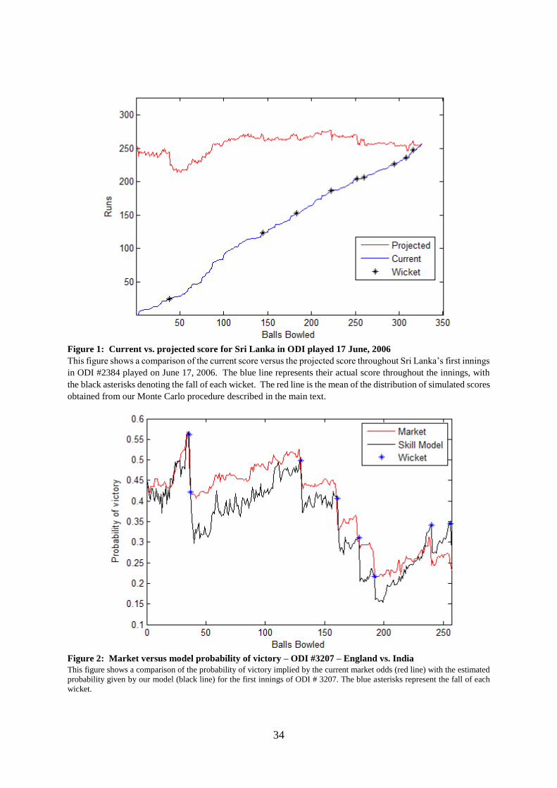
distribution. This allows us to track the projected score throughout an innings as illustrated in

the example presented in Figure 1 – the ball-by-ball projected score for Sri Lanka’s first

innings, played on 17 June, 2006.

We select an evenly spaced subset of the possible input values and construct a grid for

which simulation is both feasible and meaningful. Specifically, for each of the 101,177 balls in

our 186-game sample we run 1,000 simulations from that point until the end of the innings.25

We repeat a similar simulation process as described above to obtain the distribution of scores

at any given point in the second innings. The main difference is that the second innings ends

when Team 2 surpasses the score made by Team 1, which means that the distribution of scores

for Team 2 will be right-side truncated.

3.3.5 Probability of Victory

We convert our distribution of innings scores into probabilities of victory. For the second

innings, which is the simpler case, we substitute the current values of the input variables

𝑏, 𝑤, 𝑅𝑅𝑅, 𝑠1, 𝑠2, 𝑓, 𝐴 and 𝐾 into our simulation algorithm to obtain a distribution of scores.

We then calculate the proportion of simulated scores that are greater than or equal to Team 1’s

score and this is our estimated probability of victory for Team 2.

Estimating the probability of victory at any point during the first innings requires some

additional steps. Specifically, for each of these simulated scores we simulate 10,000 second

innings attempts at chasing that score. While at first it might seem intractable to perform

10,000 additional simulations for each of the first innings simulations, the problem becomes

much more manageable when we recognise that most of the input variables will be the same at

the start of the second innings regardless of what happened in the first innings. So we set

25 To perform this mammoth simulation exercise once took around 12 (24/7) days of solid computing time.

Although this seems like a prohibitively long time, it only takes a few seconds to run 1,000 simulations from a

given state of any one ODI game. Given that the time elapsed between each ball usually a minimum of 30 seconds

(and these are the least interesting “dot” balls), this leaves ample time for the purposes of placing wagers as part

of our trading strategies.

21

b=300, w=10, s1=0, s2=0, f=1 and then just vary RRR in order to obtain a distribution of

simulated scores for chasing each possible target. We assume that the probability of chasing

any target over 500 is equal to zero.26

We can now take each simulated first innings score and look up the corresponding

probability of Team 2 chasing it and subtract one to obtain the probability of victory for Team

1. Finally, we take the average of all of those probabilities to obtain our estimate of the

probability of victory for Team 1. It is important to point out the order in which we do this:

we calculate the probability of chasing each simulated score and then take the average of those

probabilities. This subtle difference, recognising Scwartz’ inequality, is likely to have a non-

negligible effect on the final estimate of the probability of victory.

3.4 Trading Strategies

We construct a range of trading strategies with varying levels of restrictions. All of our

strategies revolve around looking for discrepancies between the odds offered by the market and

the implied odds suggested by our model. The most basic trading strategy executes a trade

whenever the discrepancy between our model and the market odds reaches some threshold

level, which we call ‘delta’. More stringent trading rules only place trades when the odds are

particularly favourable.

To illustrate, Figure 2 shows a comparison of the market and model implied

probabilities of victory for the first innings of ODI #3207 between England and India on

October 23, 2011. The figure shows that there are situations throughout the match where there

is a substantial discrepancy between the market and model implied probabilities of victory,

particularly around the fall of a wicket. It is in these situations that we seek to place trades.

26 Given that there has only ever been one successful run chase of over 400 runs in over 3,000 ODIs we do not

expect this to affect the results.

22

We impose a trading restriction to limit the number of trades that can be placed per

innings. This is to ensure that we do not end up with a strategy unduly influenced by the

outcome of a single match. Another restriction involves only betting on games where the initial

odds discrepancy at the start of the game falls within some threshold. In some sample games,

there is a large initial discrepancy due to un-modelled factors which are likely to lead to poor

bets.27

We also implement a series of strategies that adjust our model odds to account for the

initial discrepancy. As the match progresses we expect that the market will place a greater

weight on the current state of the match and less on any pre-match differences in skill.

Accordingly, we make an adjustment equal to the initial discrepancy multiplied by the

percentage of the match that is left to be played (1st and 2nd innings, respectively):

adjustment = initial discrepancy × (1 − 0.5 ×current score

projected score) (2a)

adjustment = initial discrepancy × (0.5 − 0.5 ×current score

projected score) (2b)

The rationale behind these adjustments are as follows. In the case of (2a), at the start of the

game, we assume that the market odds are correct, whereas with (2b) we start out half way

between the model and initial odds.

Our trading strategies need to take into consideration two further factors. First, for any

bet, we need to calculate whether it is more advantageous to ‘back’ one team or ‘lay’ the other.

For example, if we believe that the market underestimates the probability of Team 1 winning

we should place a back bet on Team 1 if the following relationship holds:28

1

back 1 < (1 −

1

lay 2)

27 Such unmodelled factors include: uneven team strength and local conditions. 28 Back 1 represents the odds available to back Team 2. Lay 2 represents the odds available to lay Team 2.

23

Otherwise we should lay odds for Team 2.29

The second important consideration to make when trading on an exchange-style betting

market is the size of the spread between the available prices on either side of a trade. In

traditional financial markets this is known as the ‘bid-ask’ spread, whereas in our context it is

the ‘back-lay’ spread. The size of the spread from the mid-point essentially represents a

transaction cost when placing any bet. Consequently we avoid placing bets when this spread

is ‘overly’ large. Our trading strategies will employ a variety of different thresholds to see if

we can enhance our returns by only trading in liquid markets where the transaction costs are

low. We calculate the combined probability of Team 1 or Team 2 winning that is implied by

the available back and lay prices. While in a perfect market with no fees or transaction costs

we would expect this to equal 100%, in any market with a non-zero spread it exceeds 100%.

Finally, we note that for us to refrain from betting, the combined probability implied

by the back and lay odds must be greater than the threshold level for both Team 1 and Team 2.

As explained earlier, we can replicate any strategy of backing or laying Team 2 by backing or

laying Team 1. So as long as one of the pairs of back-lay spreads is below the threshold we

can still place a trade. There are situations where we select the odds from the wider spread

because it is a more enticing opportunity.

4. Results

4.1 Preliminaries

Unlike a typical regression situation, we do not have ‘off-the-shelf’ standard errors that we can

use to determine whether the returns generated by our trading strategies are statistically

significant. We want our p-value to represent the probability of obtaining our results purely

29 When ‘laying’ odds on a particular team, if that team ends up winning, you are liable to pay the wagered amount

multiplied by the odds at which the bet was laid. To maintain our strategy of placing a $100 bet on each game,

we lay an amount such that our net exposure is equivalent to a ‘back’ bet of $100.

24

by chance if the null hypothesis is in fact true (i.e., the Betfair market is efficient). We do this

using a bootstrap simulation procedure described below.

For each trading strategy, we simulate the payoff of an identical strategy that places the

same bets on the same team at the same odds. The key difference is that instead of the payoff

of each bet being determined by the actual outcome of the match, the result is randomly

generated such that the probability of each team winning matches the probability implied by

the market odds. For example, if we back Team 1 at odds of $2.50, the implied probability of

victory is 40%.30 We then generate a uniformly distributed random number between zero and

one and if that number is less than 40%, we treat that as a win for Team 1 and the $250 payoff

is credited to the random strategy.

We repeat this procedure for every bet placed by a given trading strategy and aggregate

the payoffs to get the total payoff for one random sample. We then repeat this process 1,000

times to get a distribution of possible payoffs for a given set of bets. The p-value is then

calculated as the proportion of those random payoffs that are greater than the actual payoff of

the strategy. In other words it is an estimate of the probability of achieving the observed returns

of a strategy purely by chance if the market odds are an unbiased estimate of the true probability

of victory.

30 prob(Team 1 win) =

1

odds to back Team 1=

1

2.50= 40%.

25

4.2 Testing the Overreaction Hypothesis (H1)

The first strategy we implement assesses hypothesis (H1) that the Betfair ‘in-play’ market

overreacts to significant news events. If the market overreacts in a manner similar to De Bondt

and Thaler (1985), a strategy of betting on the batting team immediately after the fall of a

wicket should yield positive returns. Table 4 reports the results of following this trading rule,

placing $100 wagers in the first innings under a variety of trading restrictions.31

The table shows a clear monotonically increasing relationship between the strictness of

the probability restriction and the return to the trading strategy. An unrestricted strategy (i.e.,

any probability of victory at the fall of a wicket) generates a return of -12.3% from 1,232 bets

placed. The most restrictive probability bracket of 40-60% (i.e., quite an even standing game

at the fall of a wicket) yields a return of 20.8% from 300 bets placed, significant at the 1%

level. This is strong evidence to suggest that the market overreacts to the fall of a first-innings

wicket in an economically exploitable fashion – and notably in circumstances where the fall of

the wicket is meaningful in the sense that the outcome of the game hangs in the balance.

Another interesting result from Table 4 is that the return increases when going from an

unrestricted strategy on the back-lay spread to a restriction of less than 100.75% for all five

win probability segments. That is, avoiding trades with large transaction costs, enhances

returns.32

The results from Table 4 are consistent with the idea that the market overweights news

events that occur early in the match. Given that a one-day international is usually played over

31 Throughout the paper, we examine the profitability of $100 bets and we quantify the number of bets, the total

payoffs and the return on those bets in the tables. However, what about “scalability” – what happens if a “large

stakes” wager is placed? Unfortunately, the data currently available to us include only the best three “back” and

“lay” odds at any time. That is, since we do not have the entire order book in our study, it is not possible herein

to formally assess the very interesting question of whether (or to what extent) a very large bet could have been

absorbed by the market. As such, while we acknowledge this as a limitation of our study, we identify several

countervailing factors including those mentioned briefly below. First, it is possible that a larger offer on one side

of the market may induce additional volume on the other side of the market that would not be observable to us

even if the entire order book was available. Also, we understand that large “informal” on-line betting networks

do exist that are able to absorb relatively large bets with minimal “price impact”. 32 Unlike the first innings, we find no evidence of overreaction in the second innings – these results are not reported

to conserve space. Details are available from the authors upon request.

26

a nine-hour period, there is plenty of opportunity for the momentum to shift between the two

teams and it is not uncommon for favouritism to shift from one side to another multiple times

throughout a match. It is possible that the market gets carried away with an early wicket

ignoring the fact that a large portion of the match is yet to be played.

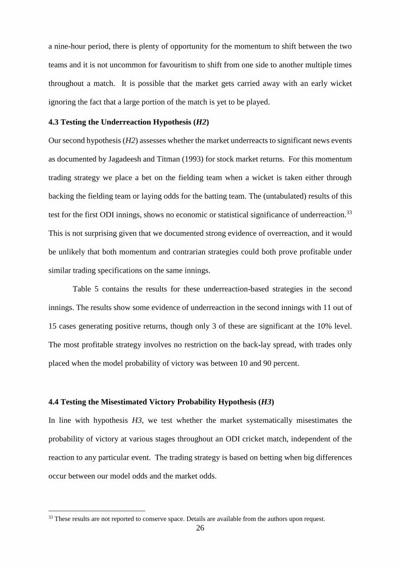
4.3 Testing the Underreaction Hypothesis (H2)

Our second hypothesis (H2) assesses whether the market underreacts to significant news events

as documented by Jagadeesh and Titman (1993) for stock market returns. For this momentum

trading strategy we place a bet on the fielding team when a wicket is taken either through

backing the fielding team or laying odds for the batting team. The (untabulated) results of this

test for the first ODI innings, shows no economic or statistical significance of underreaction.33

This is not surprising given that we documented strong evidence of overreaction, and it would

be unlikely that both momentum and contrarian strategies could both prove profitable under

similar trading specifications on the same innings.

Table 5 contains the results for these underreaction-based strategies in the second

innings. The results show some evidence of underreaction in the second innings with 11 out of

15 cases generating positive returns, though only 3 of these are significant at the 10% level.

The most profitable strategy involves no restriction on the back-lay spread, with trades only

placed when the model probability of victory was between 10 and 90 percent.

4.4 Testing the Misestimated Victory Probability Hypothesis (H3)

In line with hypothesis H3, we test whether the market systematically misestimates the

probability of victory at various stages throughout an ODI cricket match, independent of the

reaction to any particular event. The trading strategy is based on betting when big differences

occur between our model odds and the market odds.

33 These results are not reported to conserve space. Details are available from the authors upon request.

27

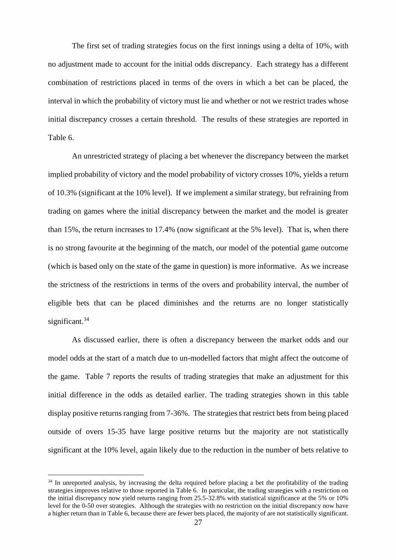
The first set of trading strategies focus on the first innings using a delta of 10%, with

no adjustment made to account for the initial odds discrepancy. Each strategy has a different

combination of restrictions placed in terms of the overs in which a bet can be placed, the

interval in which the probability of victory must lie and whether or not we restrict trades whose

initial discrepancy crosses a certain threshold. The results of these strategies are reported in

Table 6.

An unrestricted strategy of placing a bet whenever the discrepancy between the market

implied probability of victory and the model probability of victory crosses 10%, yields a return

of 10.3% (significant at the 10% level). If we implement a similar strategy, but refraining from

trading on games where the initial discrepancy between the market and the model is greater

than 15%, the return increases to 17.4% (now significant at the 5% level). That is, when there

is no strong favourite at the beginning of the match, our model of the potential game outcome

(which is based only on the state of the game in question) is more informative. As we increase

the strictness of the restrictions in terms of the overs and probability interval, the number of

eligible bets that can be placed diminishes and the returns are no longer statistically

significant.34

As discussed earlier, there is often a discrepancy between the market odds and our

model odds at the start of a match due to un-modelled factors that might affect the outcome of

the game. Table 7 reports the results of trading strategies that make an adjustment for this

initial difference in the odds as detailed earlier. The trading strategies shown in this table

display positive returns ranging from 7-36%. The strategies that restrict bets from being placed

outside of overs 15-35 have large positive returns but the majority are not statistically

significant at the 10% level, again likely due to the reduction in the number of bets relative to

34 In unreported analysis, by increasing the delta required before placing a bet the profitability of the trading

strategies improves relative to those reported in Table 6. In particular, the trading strategies with a restriction on

the initial discrepancy now yield returns ranging from 25.5-32.8% with statistical significance at the 5% or 10%

level for the 0-50 over strategies. Although the strategies with no restriction on the initial discrepancy now have

a higher return than in Table 6, because there are fewer bets placed, the majority of are not statistically significant.

28

the unrestricted strategies. All ten unrestricted strategies are statistically significant at a

minimum 10% level. Interestingly, a strategy that restricts bets to when the probability of

victory is between 40 and 60 percent, yields a return of 36.2% which is significant at the 1%

level. This is strong evidence that inefficiencies may exist in the ‘in-play’ Betfair market for

ODIs.

When the Table 7 analysis is repeated for a delta of 15% (unreported), no strategy is

statistically significant at the 10% level. This result is not surprising given that a delta of 15%

is going to occur much less frequently than in Table 7, since we have adjusted the model odds

to account for the initial discrepancy between the market and the model. With such a reduction

in the number of bets in each strategy, it is much more difficult to find significant results.

In our final test, a similar set of trading strategies on the second ODI innings are

analysed and Table 8 reports the results for the 10% delta case, with no initial odds adjustment.

While all trading strategies show positive economic returns, only the strategies that restrict bets

from being placed outside of overs 15-35 are statistically significant.35 One possible

explanation for this is that the latter stages of the second innings will likely be influenced by

game specific factors that are not taken into account in our model.36

A further reason that our model might not perform as well towards the very end of the

game is that the career batting averages and strike rates in our model will convey limited

information in the final stages of a game. By then, the majority of players will have batted and

most of the overs will have been completed so that the career statistics are of little consequence.

35 In unreported analysis, we apply an initial odds adjustment to the second innings sample in a comparable way

to Table 7 for the first innings. This produces a negative return to all trading strategies for the second innings.

This is not unexpected since the relative importance of any pre-match differences in skill that were factored in to

the market odds at the start of the match will diminish as the match progresses. 36 For example, if a team requires 20 runs off 2 overs to win the game, factors such as the ‘Death bowling’ ability

of the remaining bowlers and the ability of the batsman to play under pressure becomes important. While we

would expect the market to take these factors into account, capturing this would be difficult as it would require

the model to keep track of how many overs each bowler has bowled, as well as having some sort of death bowling

and pressure batting rating for each player.

29

5. Conclusions

This study tests a range of trading strategies using the ‘in-play’ Betfair market for ODI cricket

games. Unlike a traditional financial market, such sports betting markets provide an ideal

setting for these tests because the true value of the asset is revealed at a definite ending point.

An ‘in-play’ cricket betting market is especially comparable to a traditional financial market

because there is regular sequence of ‘news events’ (in the form of the outcome of each delivery)

that must be priced by the market. This allows us to unambiguously measure the market’s

perception of the impact of the information arrival to determine if the market reacts in a rational

and efficient manner. Our method utilises information at the ball-by-ball level to estimate the

model parameters. While ball-by-ball histories been recorded for all one-day internationals

since 2001, it is only with major advances in computer technology in very recent times, that

there is now sufficient accessible data to obtain reliable parameter estimates. But as explained

in the paper, simulation of game scenarios with the richness/depth of models that we employ

is no trivial task and our solutions to these challenges represent major breakthroughs in this

literature.

We construct a series of momentum and contrarian strategies designed to exploit any

systematic biases in the markets reaction to the outcome of each ball. We also examine if the

market systematically misestimates the probability of victory throughout a cricket match

independent of their reaction to a single news event. To the best of our knowledge, ours is the

first study to factor in player-specific characteristics of any sort to determine the probability of

victory at any point in a match. To achieve this last goal we require a model to estimate what

impact a particular news event should have on the market odds. Specifically, we develop a

Monte Carlo simulation procedure to estimate a distribution of scores from any possible match

situation. Our key results are summarised below.

The most successful strategy in terms of both economic and statistical significance is

achieved in the first innings by placing bets when the batting side had a probability of victory

30

between 40 and 60 percent and when the combined spread was less than 100.75%. This

overreaction-based strategy yields an after-commission return of 20.8%, significant at the 1%

level. In the second innings we find evidence that the market underreacts to the fall of a wicket.

The most profitable return is achieved by betting on the fielding team to win immediately after

the fall of a wicket as long as the batting team’s probability of victory is between 20 and 80

percent and the combined spread is less than 100.50%. This strategy achieves an after-

commission return of 9.3%.

Regarding whether the market systematically misestimates the probability of victory,

we document several profitable trading strategies in the first and second innings. The most

profitable first innings trading strategy is achieved with a delta of 10% and a restriction on

placing bets when the model probability of victory is outside of the 40 to 60 percent range.

This strategy generates a return of 38.6%, significant at the 1% level. Overall, these results

suggest that the ‘Betfair’ market does not satisfy the definition of weak-form efficiency

suggested by Thaler and Ziemba (1988).

In ongoing research, we are considering a number of ways to further refine our dynamic

programming model. First, whereas we condition on the full career average score of each

batsman (which we argue to be a substantial and an important improvement on existing models)

there might be additional relevant information in more recent batting “form”, such as the

batting average over the last six or twelve months or over the previous dozen matches.

Inclusion of this “batting form” variable would allow us to examine behavioural biases such as

the tendency to over-weight more recent observations. Second, whereas we currently condition

on the “quality” of each batsman, the model could be extended to also condition on the quality

of each bowler. As argued above, such a bowling focus is expected to have a smaller effect.

Third, we also note that the rules relating to “power plays” varied over our sample period.37

37 In ODIs, the batting team receives a five-over “power play”, during which the fielding team is restricted in the

number of fielders it is allowed to place near the boundary of the playing field. This feature is designed to allow

the batting team to score at a faster rate than is otherwise possible.

31

Whether or not a team has used its power play could be included as an additional conditioning

variable in the model. Finally, the model could also be extended to incorporate variables that

relate to the general circumstances of the game – for example, whether one of the teams is

playing at home, whether the game is “alive” or just part of series that has already be decided,

and whether the game is a standard fixture or some sort of final.

32

References Ali, M.M. 1977. Probability and utility estimates for racetrack bettors. Journal of Political Economy

85(4): 803-815.

Asch, P., Malkiel, B.G. and Quandt, B.1982. Racetrack betting and informed behaviour. Journal of

Financial Economics 10:187-194.

Bailey, M.J. 2005. Predicting sporting outcomes: a statistical approach. PHD Thesis, Swinburne

University of Technology, Melbourne.

Bailey, M. and Clarke, S. 2006. Predicting the match outcome in one-day international cricket matches,

while the game is in progress. Journal of Sports Science and Medicine 5: 480-487.

Bairam, E., Howells, J. and Turner, G. 2006. Production functions in cricket: The Australian and New

Zealand Experience. Applied Economics 22(7): 871-879.

Brailsford, T.J., Gray, P.K., Easton, S.A. and Gray, S.F. 1995. The efficiency of Australian Football

betting markets. Australian Journal of Management 20: 167-197.

Brooker, S. 2009. Determining batting production possibility frontiers in One-Day International (ODI)

cricket. New Zealand Association of Economists Conference, Christchurch.

Brooker, S. and Hogan, S. 2011. A method for inferring batting conditions in ODI cricket form historical

data. University of Canterbury- Department of Economics and Finance, Working Paper.

Brown, A. 2012. Evidence of in-play insider trading on a UK betting exchange. Applied Economics

44(9): 1169-1175

Carter, M. and Guthrie, G. 2004. Cricket Interruptus: Fairness and Incentive in Limited Overs Cricket

Matches. The Journal of the Operational Research Society 55(8): 822-829.

-----------. Reply to the Comments of Duckworth and Lewis. The Journal of the Operational Research

Society 56(11): 1337-1341.

Clarke, R. 1988. Dynamic Programming in One-Day Cricket-Optimal Scoring Rates. The Journal of

the Operational Research Society 39(4): 331-337.

Dare, W.H. and Holland, S. 2004. Efficiency in the NFL betting market: modifying and consolidating

research methods. Applied Economics 36(1): 9-15.

Dasgupta, S. 2013. It’s always been a batsman’s game. Wisden India,

http://www.wisdenindia.com/cricket-blog/its-batsmans-game/84531 (accessed 9 July 2015).

De Bondt, W.F. and Thaler, R. 1985. Does the stock market overreact? The Journal of Finance 40(3):

28-30.

Demir, E., Danis, H. and Rigoni, U. 2012. Is the soccer betting market efficient? A cross-country

investigation using the Fibonacci strategy. The Journal of Gambling Business and Economics 6(2):

29-49.

Docherty, P. and Easton, S. 2012. Market efficiency and continuous information arrival: evidence from

prediction markets. Applied Economics 44(19): 2461-2471.

Duckworth, F.C. and Lewis, A.J. 1998. A fair method for resetting the target in interrupted one-day

cricket matches. Journal of the Operational Research Society 49: 230-237.

------------. 2005. Comment on Carter and Guthrie (2004). Cricket Interruptus: Fairness and Incentive

in Limited Overs Cricket Matches. Journal of the Operational Research Society 56(11): 1333-

1337.

Easton, S. and Uylangco, K. 2006. An examination of in-play sports betting using one-day cricket

matches. University of Newcastle- School of Business and Management, Callaghan.

Forrest, D. and McHale, I. 2007. Anyone for Tennis (Betting)? The European Journal of Finance 13(8):

751-768.

Gray, P.K. and Gray, S.F. 1997. Testing market efficiency Evidence from NFL Sports Betting Market.

The Journal of Finance 52(4): 1725-1737.

Golec, J. and Tamarkin, M. 1991. The degree of inefficiency in the football betting market. Journal of

Financial Economics 30: 311-323.

Griffith, R.M. 1949. Odds adjustments by American Horse-Race bettors. The American Journal of

Psychology 62(2): 290-294.

Jagadeesh, N. and Titman, S. 1993. Returns to Buying Winners and Selling Losers: Implications for

Stock Market Efficiency. The Journal of Finance 48(1): 65-91.

Johnston, M., Clarke, S. and Noble, D. 1993. Assessing player performance in one-day cricket using

dynamic programming. Asia Pacific Journal of Operational Research 10: 45-55.

McGlothin, W.H. 1956. Stability of Choices among Uncertain Alternatives. The American Journal of

33

Psychology 69(4): 604-615.

Norman, J. and Clarke, S. 2007. Dynamic Programming in Cricket: Optimizing Batting Order for a

Sticky Cricket. The Journal of Operational Research Society 58(12): 1678-1982.

Norman, J. and Clarke, S. 2010. Optimal batting orders in cricket. Journal of the Operational Research

Society 61: 980-986.

Paul, R.J. and Weinbach, A.P. 2008. Line movements and market timing the baseball gambling market.

Journal of Sports Economics 9: 371-388.

Paul, R.J. and Weinbach, A.P. 2008. Price setting in the NBA gambling market: Tests of the Levitt

Model of Sportsbook behaviour. Journal of Sports Economics 3: 137-145.

Preston, I. and Thomas, J. 2000. Batting Strategy in Limited Overs Cricket. Journal of the Royal

Statistical Society 49(1): 95-106.

Ovens, M. and Bukiet, B.A. 2006. Mathematical Modelling Approach to One-Day Cricket Batting

Orders. Journal of Sports Science and Medicine 5: 295-502.

Ryall, R. and Bedford, A. 2010. The efficiency of ‘In-Play’ Australian Rules Football betting markets.

International Journal of Sport Finance 5: 193-207.

Snyder, W. 1978. Horse Racing: Testing the Efficient Markets Model. The Journal of Finance 33(4):

1109-1118.

Swartz, T.B., Gill, P.S. Muthukumarana, S. 2009. Modelling and simulation for one-day cricket. The

Canadian Journal of Statistics 37(2): 143-160.

Thaler, R. and Ziemba, W. 1988. Anomalies: Parimutuel Betting Markets: Racetracks and Lotteries.

The Journal of Economic Perspectives 2(2): 161-174.

Weitzman, M. 1965. Utility Analysis and Group Behavior: An Empirical Study. Journal of Political

Economy 73(1): 18-26.

Ziemba, W.T. and Hausch, D.B. 1987. Beat the Racetrack. Harcourt, San Francisco.

34

Figure 1: Current vs. projected score for Sri Lanka in ODI played 17 June, 2006

This figure shows a comparison of the current score versus the projected score throughout Sri Lanka’s first innings

in ODI #2384 played on June 17, 2006. The blue line represents their actual score throughout the innings, with

the black asterisks denoting the fall of each wicket. The red line is the mean of the distribution of simulated scores

obtained from our Monte Carlo procedure described in the main text.

Figure 2: Market versus model probability of victory – ODI #3207 – England vs. India

This figure shows a comparison of the probability of victory implied by the current market odds (red line) with the estimated

probability given by our model (black line) for the first innings of ODI # 3207. The blue asterisks represent the fall of each

wicket.

35

Table 1: Distribution of Ball Outcomes This table presents the observed frequency of ball outcomes in our full sample of 1,101 ODI

matches played between June 2001 and March 2013. Byes and leg byes are treated as runs scored

by the batsman.

Innings 1 Innings 2

Outcome Frequency % Frequency % Total

No. Obs

Wicket 8,629 2.7% 7,249 2.6% 15,878

Wide 6,399 2.0% 5,639 2.0% 12,038

No-ball 1,342 0.4% 1,305 0.5% 2,647

0 runs 157,068 48.6% 138,657 49.8% 295,725

1 run 103,218 31.9% 84,497 30.4% 187,715

2 runs 18,463 5.7% 15,262 5.5% 33,725

3 runs 2,480 0.8% 2,309 0.8% 4,789

4 runs 22,090 6.8% 20,241 7.3% 42,331

5 runs 504 0.2% 468 0.2% 972

6 runs 3,256 1.0% 2,621 0.9% 5,877

7 runs 22 0.0% 25 0.0% 47

Total 323,471 278,273 601,744

36

Table 2: Estimates for the Wickets Process for ODI Innings 1 This table shows the coefficient estimates for the probit model, modelling the likelihood of a wicket occurring on

the next ball bowled. The explanatory variables are: Balls – number of balls remaining in the innings; Wicket –

number of wickets remaining for the batting team; Score – current score of the batsman on strike; Av/SR – on

strike batsman's career batting average divided by his career strike rate. The coefficients are separately estimated

for each of the 15 innings/wickets segments. The first column shows the number of sample observations that

occur in each bivariate segment in the actual dataset. ***, ** and * indicate significance at 1%, 5% and 10%

levels, respectively.

Seg

Num # Obs

Over

Segment

Wicket

Segment

constant

(β0)

Balls

(β1)

Wicket

(β2)

Score

(β3)

Av/SR

(β4)

1 34,507 1-15 0 -1.015 -0.002 - 0.001 -0.013***

2 40,227 1-15 1-2 -1.506 -0.001 0.026 -0.001 -0.013***

3 8,522 1-15 3-9 -1.976 -0.001 0.109** 0.008** -0.012***

4 43,409 16-35 0-2 -1.848 0.000 0.018 0.001* -0.009***

5 44,565 16-35 3-4 -1.941 0.001** -0.008 0.003*** -0.008***

6 20,503 16-35 5-9 -1.566 0.000 -0.022 0.003** -0.011***

7 8,716 36-40 0-3 -1.856 -0.004 0.074* 0.001 -0.007**

8 10,445 36-40 4-5 -1.578 -0.004 0.071 0.003** -0.015***

9 6,525 36-40 6-9 -0.939 -0.007* -0.061* 0.002 -0.010**

10 9,607 41-45 0-4 -1.706 -0.005* 0.067** 0.002** -0.007***

11 9,464 41-45 5-6 -1.404 -0.005 -0.005 0.001 -0.007**

12 5,395 41-45 7-9 -1.154 -0.007** -0.040 0.003 -0.010**

13 8,050 46-50 0-5 -1.245 -0.007*** 0.005 0.002*** -0.006***

14 8,290 46-50 6-7 -1.168 -0.021*** 0.072* 0.002** -0.008***

15 5,288 46-50 8-9 -0.900 -0.027*** 0.020 -0.001 -0.007*

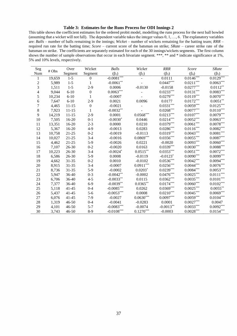
37

Table 3: Estimates for the Runs Process for ODI Innings 2 This table shows the coefficient estimates for the ordered probit model, modelling the runs process for the next ball bowled

(assuming that a wicket will not fall). The dependent variable takes the integer values 0, 1, …, 6. The explanatory variables

are: Balls – number of balls remaining in the innings; Wicket – number of wickets remaining for the batting team; RRR –

required run rate for the batting time; Score – current score of the batsman on strike; SRate – career strike rate of the

batsman on strike. The coefficients are separately estimated for each of the 30 innings/wickets segments. The first column

shows the number of sample observations that occur in each bivariate segment. ***, ** and * indicate significance at 1%,

5% and 10% levels, respectively.

Seg

Num # Obs

Over

Segment

Wicket

Segment

Balls

(β1)

Wicket

(β2)

RRR

(β3)

Score

(β4)

SRate

(β5)

1 19,659 1-5 0 -0.0081*** - 0.0111 0.0146*** 0.0129***

2 5,989 1-5 1 -0.0061** - 0.0447*** 0.0211*** 0.0063***

3 1,511 1-5 2-9 0.0006 -0.0130 -0.0158 0.0277*** 0.0112**

4 9,044 6-10 0 0.0063*** - 0.0233*** 0.0131*** 0.0083***

5 10,234 6-10 1 -0.0007 - 0.0279*** 0.0119*** 0.0070***

6 7,647 6-10 2-9 0.0021 0.0096 0.0177 0.0172*** 0.0051**

7 4,465 11-15 0 -0.0021 - 0.0331*** 0.0059*** 0.0125***

8 7,923 11-15 1 -0.0032** - 0.0268*** 0.0077*** 0.0110***

9 14,219 11-15 2-9 0.0001 0.0568*** 0.0213*** 0.0107*** 0.0079***

10 7,505 16-20 0-1 -0.0030* 0.0446 0.0214*** 0.0052*** 0.0063***

11 13,351 16-20 2-3 0.0000 0.0210 0.0379*** 0.0061*** 0.0078***

12 5,367 16-20 4-9 -0.0013 0.0283 0.0286*** 0.0116*** 0.0082***

13 10,758 21-25 0-2 -0.0019 -0.0113 0.0319*** 0.0043*** 0.0081***

14 10,027 21-25 3-4 -0.0016 0.0869*** 0.0356*** 0.0055*** 0.0087***

15 4,462 21-25 5-9 -0.0026 0.0221 -0.0020 0.0093*** 0.0060***

16 7,107 26-30 0-2 -0.0020 0.0163 0.0339*** 0.0030*** 0.0088***

17 10,223 26-30 3-4 -0.0024* 0.0515** 0.0353*** 0.0051*** 0.0072***

18 6,586 26-30 5-9 0.0008 -0.0119 -0.0123* 0.0090*** 0.0099***

19 4,662 31-35 0-2 0.0010 -0.0102 0.0536*** 0.0042*** 0.0094***

20 8,915 31-35 3-4 -0.0007 0.0911*** 0.0256*** 0.0044*** 0.0076***

21 8,736 31-35 5-9 -0.0002 0.0203* 0.0239*** 0.0084*** 0.0053***

22 5,947 36-40 0-3 -0.0042** -0.0002 0.0476*** 0.0025*** 0.0111***

23 6,706 36-40 4-5 -0.0033** 0.0115 0.0362*** 0.0035*** 0.0101***

24 7,377 36-40 6-9 -0.0039** 0.0365** 0.0174*** 0.0060*** 0.0102***

25 5,118 41-45 0-4 -0.0085*** 0.0262 0.0369*** 0.0025*** 0.0055**

26 5,437 41-45 5-6 -0.0053*** 0.0008 0.0210*** 0.0045*** 0.0069***

27 6,076 41-45 7-9 -0.0027 0.0630*** 0.0097*** 0.0059*** 0.0104***

28 1,319 46-50 0-4 -0.0041 -0.0283 0.0001 0.0027*** 0.0047

29 4,101 46-50 5-7 -0.0083*** -0.0074 -0.0013** 0.0033*** 0.0092***

30 3,743 46-50 8-9 -0.0108*** 0.1270*** -0.0003 0.0028*** 0.0154***

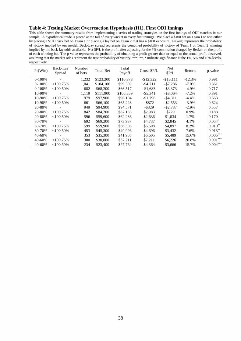
38

Table 4: Testing Market Overreaction Hypothesis (H1), First ODI Innings This table shows the summary results from implementing a series of trading strategies on the first innings of ODI matches in our

sample. A hypothetical trade is placed at the fall of every wicket in every first innings. We place a $100 bet on Team 1 to win either

by placing a $100 back bet on Team 1 or placing a lay bet on Team 2 that has a $100 exposure. Pr(win) represents the probability

of victory implied by our model. Back-Lay spread represents the combined probability of victory of Team 1 or Team 2 winning

implied by the back-lay odds available. Net $P/L is the profit after adjusting for the 5% commission charged by Betfair on the profit

of each winning bet. The p-value represents the probability of obtaining a profit greater than or equal to the actual profit observed,

assuming that the market odds represent the true probability of victory. ***, **, * indicate significance at the 1%, 5% and 10% levels,

respectively.

Pr(Win) Back-Lay

Spread

Number

of bets Total Bet

Total

Payoff Gross $P/L

Net

$P/L Return p-value

0-100% - 1,232 $123,200 $110,878 -$12,322 -$15,111 -12.3% 0.991

0-100% <100.75% 1,041 $104,100 $99,389 -$4,711 -$7,286 -7.0% 0.861

0-100% <100.50% 682 $68,200 $66,517 -$1,683 -$3,373 -4.9% 0.717

10-90% - 1,119 $111,900 $106,559 -$5,341 -$8,064 -7.2% 0.891

10-90% <100.75% 979 $97,900 $96,104 -$1,796 -$4,311 -4.4% 0.663

10-90% <100.50% 661 $66,100 $65,228 -$872 -$2,553 -3.9% 0.624

20-80% - 949 $94,900 $94,571 -$329 -$2,737 -2.9% 0.557

20-80% <100.75% 842 $84,200 $87,183 $2,983 $729 0.9% 0.188

20-80% <100.50% 596 $59,600 $62,236 $2,636 $1,034 1.7% 0.170

30-70% - 692 $69,200 $73,937 $4,737 $2,845 4.1% 0.054 *

30-70% <100.75% 599 $59,900 $66,508 $6,608 $4,897 8.2% 0.010 **

30-70% <100.50% 453 $45,300 $49,996 $4,696 $3,432 7.6% 0.013 **

40-60% - 353 $35,300 $41,905 $6,605 $5,489 15.6% 0.005 ***

40-60% <100.75% 300 $30,000 $37,211 $7,211 $6,226 20.8% 0.001 ***

40-60% <100.50% 234 $23,400 $27,764 $4,364 $3,666 15.7% 0.004 ***

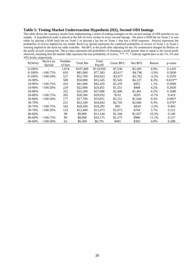
39

Table 5: Testing Market Underreaction Hypothesis (H2), Second ODI Innings This table shows the summary results from implementing a series of trading strategies on the second innings of ODI matches in our

sample. A hypothetical trade is placed at the fall of every wicket in every second innings. We place a $100 bet on Team 2 to win

either by placing a $100 back bet on Team 2 or placing a lay bet on Team 1 that has a $100 exposure. Pr(win) represents the

probability of victory implied by our model. Back-Lay spread represents the combined probability of victory of Team 1 or Team 2

winning implied by the back-lay odds available. Net $P/L is the profit after adjusting for the 5% commission charged by Betfair on

the profit of each winning bet. The p-value represents the probability of obtaining a profit greater than or equal to the actual profit

observed, assuming that the market odds represent the true probability of victory. ***, **, * indicate significance at the 1%, 5% and

10% levels, respectively.

Pr(Win) Back-Lay

Spread

Number

of bets Total Bet

Total

Payoff Gross $P/L Net $P/L Return p-value

0-100% - 1,074 $107,400 $114,936 $7,536 $5,269 4.9% 0.1410

0-100% <100.75% 810 $81,000 $77,383 -$3,617 -$4,796 -5.9% 0.5830

0-100% <100.50% 527 $52,700 $50,623 -$2,077 -$2,763 -5.2% 0.3550

10-90% - 500 $50,000 $55,545 $5,545 $4,127 8.3% 0.033**

10-90% <100.75% 410 $41,000 $42,470 $1,470 $452 1.1% 0.2690

10-90% <100.50% 229 $22,900 $24,451 $1,551 $968 4.2% 0.2050

20-80% - 352 $35,200 $37,606 $2,406 $1,461 4.2% 0.1680

20-80% <100.75% 285 $28,500 $29,032 $532 -$205 -0.7% 0.419

20-80% <100.50% 177 $17,700 $19,851 $2,151 $1,644 9.3% 0.083*

30-70% - 221 $22,100 $24,843 $2,743 $2,066 9.3% 0.076*

30-70% <100.75% 182 $18,200 $18,295 $95 -$410 -2.3% 0.443

30-70% <100.50% 124 $12,400 $13,473 $1,073 $704 5.7% 0.212

40-60% - 98 $9,800 $11,144 $1,344 $1,027 10.5% 0.140

40-60% <100.75% 89 $8,900 $10,175 $1,275 $986 11.1% 0.157

40-60% <100.50% 63 $6,300 $6,791 $491 $302 4.8% 0.288

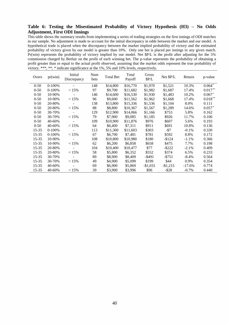
40

Table 6: Testing the Misestimated Probability of Victory Hypothesis (H3) – No Odds

Adjustment, First ODI Innings This table shows the summary results from implementing a series of trading strategies on the first innings of ODI matches

in our sample. No adjustment is made to account for the initial discrepancy in odds between the market and our model. A

hypothetical trade is placed when the discrepancy between the market implied probability of victory and the estimated

probability of victory given by our model is greater than 10%. Only one bet is placed per innings in any given match.

Pr(win) represents the probability of victory implied by our model. Net $P/L is the profit after adjusting for the 5%

commission charged by Betfair on the profit of each winning bet. The p-value represents the probability of obtaining a

profit greater than or equal to the actual profit observed, assuming that the market odds represent the true probability of

victory. ***, **, * indicate significance at the 1%, 5% and 10% levels, respectively.

Overs pr(win) Initial

Discrepancy

Num

bets Total Bet

Total

Payoff

Gross

$P/L Net $P/L Return p-value

0-50 0-100% - 148 $14,800 $16,770 $1,970 $1,521 10.3% 0.064 *

0-50 0-100% < 15% 97 $9,700 $11,682 $1,982 $1,687 17.4% 0.017 **

0-50 10-90% - 146 $14,600 $16,530 $1,930 $1,483 10.2% 0.067 *

0-50 10-90% < 15% 96 $9,600 $11,562 $1,962 $1,668 17.4% 0.018 **

0-50 20-80% - 138 $13,800 $15,336 $1,536 $1,104 8.0% 0.111

0-50 20-80% < 15% 88 $8,800 $10,367 $1,567 $1,289 14.6% 0.057 *

0-50 30-70% - 129 $12,900 $14,066 $1,166 $753 5.8% 0.162

0-50 30-70% < 15% 79 $7,900 $9,085 $1,185 $926 11.7% 0.106

0-50 40-60% - 109 $10,900 $11,876 $976 $607 5.6% 0.193

0-50 40-60% < 15% 64 $6,400 $7,311 $911 $691 10.8% 0.136

15-35 0-100% - 113 $11,300 $11,603 $303 -$7 -0.1% 0.330

15-35 0-100% < 15% 67 $6,700 $7,481 $781 $592 8.8% 0.172

15-35 10-90% - 108 $10,800 $10,980 $180 -$124 -1.1% 0.366

15-35 10-90% < 15% 62 $6,200 $6,858 $658 $475 7.7% 0.198

15-35 20-80% - 104 $10,400 $10,477 $77 -$222 -2.1% 0.409

15-35 20-80% < 15% 58 $5,800 $6,352 $552 $374 6.5% 0.233

15-35 30-70% - 89 $8,900 $8,409 -$491 -$751 -8.4% 0.564

15-35 30-70% < 15% 49 $4,900 $5,099 $199 $44 0.9% 0.354

15-35 40-60% - 69 $6,900 $5,869 -$1,031 -$1,215 -17.6% 0.774

15-35 40-60% < 15% 39 $3,900 $3,996 $96 -$28 -0.7% 0.440

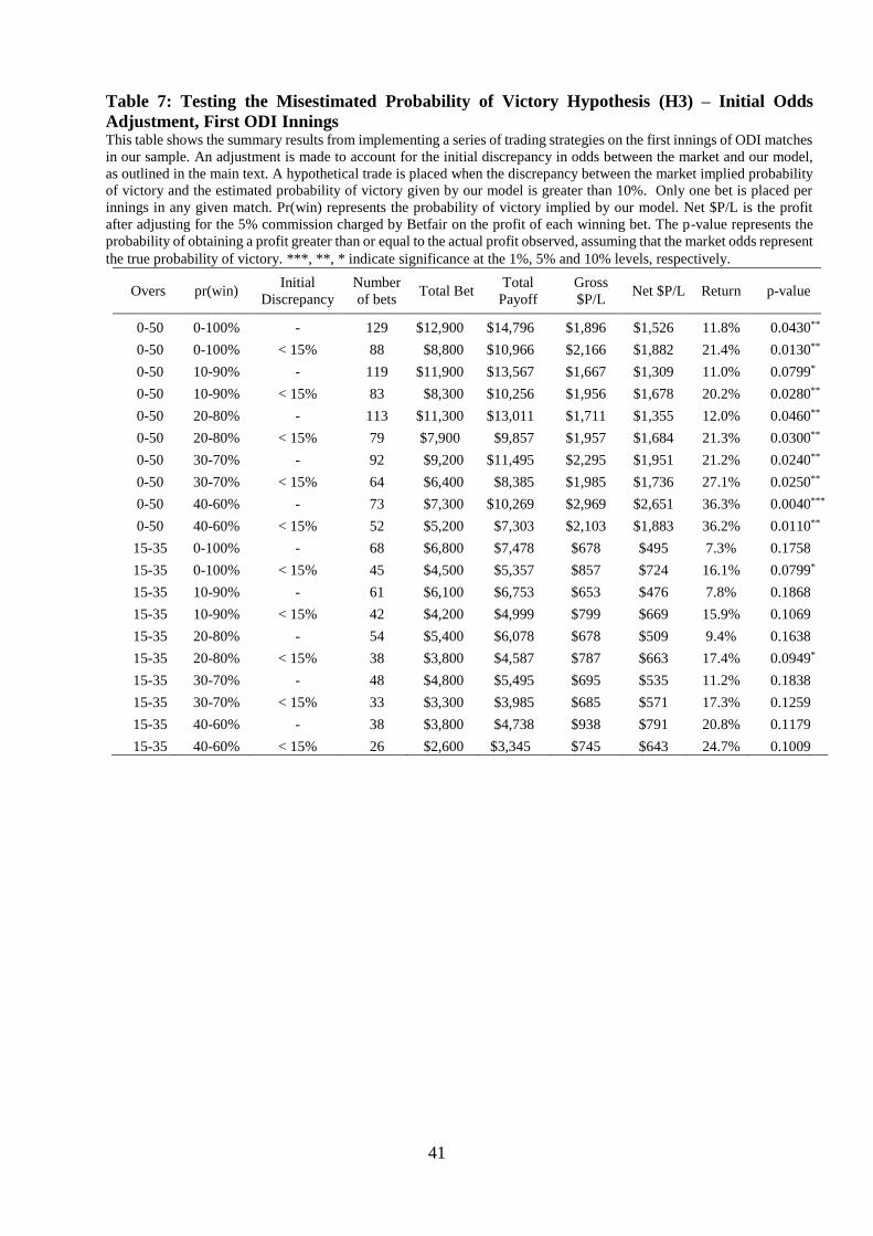
41

Table 7: Testing the Misestimated Probability of Victory Hypothesis (H3) – Initial Odds

Adjustment, First ODI Innings This table shows the summary results from implementing a series of trading strategies on the first innings of ODI matches

in our sample. An adjustment is made to account for the initial discrepancy in odds between the market and our model,

as outlined in the main text. A hypothetical trade is placed when the discrepancy between the market implied probability

of victory and the estimated probability of victory given by our model is greater than 10%. Only one bet is placed per

innings in any given match. Pr(win) represents the probability of victory implied by our model. Net $P/L is the profit

after adjusting for the 5% commission charged by Betfair on the profit of each winning bet. The p-value represents the

probability of obtaining a profit greater than or equal to the actual profit observed, assuming that the market odds represent

the true probability of victory. ***, **, * indicate significance at the 1%, 5% and 10% levels, respectively.

Overs pr(win) Initial

Discrepancy

Number

of bets Total Bet

Total

Payoff

Gross

$P/L Net $P/L Return p-value

0-50 0-100% - 129 $12,900 $14,796 $1,896 $1,526 11.8% 0.0430 **

0-50 0-100% < 15% 88 $8,800 $10,966 $2,166 $1,882 21.4% 0.0130 **

0-50 10-90% - 119 $11,900 $13,567 $1,667 $1,309 11.0% 0.0799 *

0-50 10-90% < 15% 83 $8,300 $10,256 $1,956 $1,678 20.2% 0.0280 **

0-50 20-80% - 113 $11,300 $13,011 $1,711 $1,355 12.0% 0.0460 **

0-50 20-80% < 15% 79 $7,900 $9,857 $1,957 $1,684 21.3% 0.0300 **

0-50 30-70% - 92 $9,200 $11,495 $2,295 $1,951 21.2% 0.0240 **

0-50 30-70% < 15% 64 $6,400 $8,385 $1,985 $1,736 27.1% 0.0250 **

0-50 40-60% - 73 $7,300 $10,269 $2,969 $2,651 36.3% 0.0040 ***

0-50 40-60% < 15% 52 $5,200 $7,303 $2,103 $1,883 36.2% 0.0110 **

15-35 0-100% - 68 $6,800 $7,478 $678 $495 7.3% 0.1758

15-35 0-100% < 15% 45 $4,500 $5,357 $857 $724 16.1% 0.0799 *

15-35 10-90% - 61 $6,100 $6,753 $653 $476 7.8% 0.1868

15-35 10-90% < 15% 42 $4,200 $4,999 $799 $669 15.9% 0.1069

15-35 20-80% - 54 $5,400 $6,078 $678 $509 9.4% 0.1638

15-35 20-80% < 15% 38 $3,800 $4,587 $787 $663 17.4% 0.0949 *

15-35 30-70% - 48 $4,800 $5,495 $695 $535 11.2% 0.1838

15-35 30-70% < 15% 33 $3,300 $3,985 $685 $571 17.3% 0.1259

15-35 40-60% - 38 $3,800 $4,738 $938 $791 20.8% 0.1179

15-35 40-60% < 15% 26 $2,600 $3,345 $745 $643 24.7% 0.1009

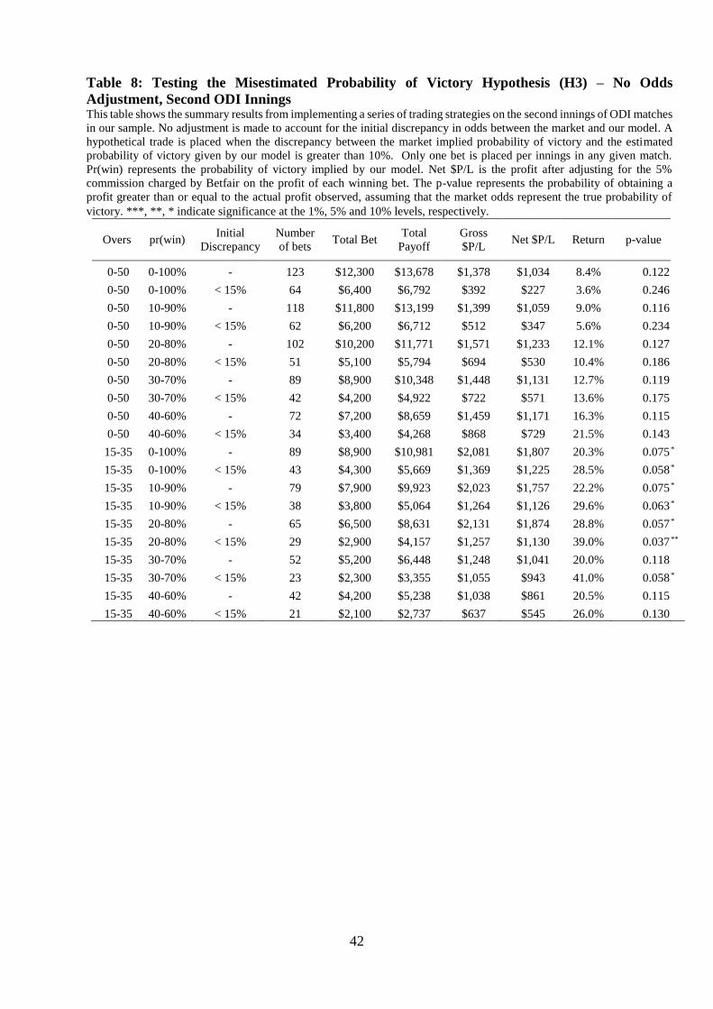
42

Table 8: Testing the Misestimated Probability of Victory Hypothesis (H3) – No Odds

Adjustment, Second ODI Innings This table shows the summary results from implementing a series of trading strategies on the second innings of ODI matches

in our sample. No adjustment is made to account for the initial discrepancy in odds between the market and our model. A

hypothetical trade is placed when the discrepancy between the market implied probability of victory and the estimated

probability of victory given by our model is greater than 10%. Only one bet is placed per innings in any given match.

Pr(win) represents the probability of victory implied by our model. Net $P/L is the profit after adjusting for the 5%

commission charged by Betfair on the profit of each winning bet. The p-value represents the probability of obtaining a

profit greater than or equal to the actual profit observed, assuming that the market odds represent the true probability of

victory. ***, **, * indicate significance at the 1%, 5% and 10% levels, respectively.

Overs pr(win) Initial

Discrepancy

Number

of bets Total Bet

Total

Payoff

Gross

$P/L Net $P/L Return p-value

0-50 0-100% - 123 $12,300 $13,678 $1,378 $1,034 8.4% 0.122

0-50 0-100% < 15% 64 $6,400 $6,792 $392 $227 3.6% 0.246

0-50 10-90% - 118 $11,800 $13,199 $1,399 $1,059 9.0% 0.116

0-50 10-90% < 15% 62 $6,200 $6,712 $512 $347 5.6% 0.234

0-50 20-80% - 102 $10,200 $11,771 $1,571 $1,233 12.1% 0.127

0-50 20-80% < 15% 51 $5,100 $5,794 $694 $530 10.4% 0.186

0-50 30-70% - 89 $8,900 $10,348 $1,448 $1,131 12.7% 0.119

0-50 30-70% < 15% 42 $4,200 $4,922 $722 $571 13.6% 0.175

0-50 40-60% - 72 $7,200 $8,659 $1,459 $1,171 16.3% 0.115

0-50 40-60% < 15% 34 $3,400 $4,268 $868 $729 21.5% 0.143

15-35 0-100% - 89 $8,900 $10,981 $2,081 $1,807 20.3% 0.075 *

15-35 0-100% < 15% 43 $4,300 $5,669 $1,369 $1,225 28.5% 0.058 *

15-35 10-90% - 79 $7,900 $9,923 $2,023 $1,757 22.2% 0.075 *

15-35 10-90% < 15% 38 $3,800 $5,064 $1,264 $1,126 29.6% 0.063 *

15-35 20-80% - 65 $6,500 $8,631 $2,131 $1,874 28.8% 0.057 *

15-35 20-80% < 15% 29 $2,900 $4,157 $1,257 $1,130 39.0% 0.037 **

15-35 30-70% - 52 $5,200 $6,448 $1,248 $1,041 20.0% 0.118

15-35 30-70% < 15% 23 $2,300 $3,355 $1,055 $943 41.0% 0.058 *

15-35 40-60% - 42 $4,200 $5,238 $1,038 $861 20.5% 0.115

15-35 40-60% < 15% 21 $2,100 $2,737 $637 $545 26.0% 0.130

43

Appendix

A1. Brief Description of One-day Cricket

Due to the complicated nature of one-day international cricket, only rules central to this paper

will be explained. A one-day international is contested between two teams of 11 players each.

The game is split into two main phases known as “innings”. In each innings, the batting team

is allotted 50 overs (each over consisting of 6 legal deliveries or “balls” bowled to them by the

opposing team) and 10 wickets with which to score as many runs as possible. When either 50

overs have been bowled or 10 wickets have been lost, the innings is complete and the teams

switch roles for the second innings. While an individual batsman is allowed to bat for the entire

50 overs allotted to his team with no limit on his score, no one bowler can bowl more than 20%

of the total overs available in any given ODI innings.

For each ball bowled, the outcome will either be a wicket, no run, one run, two runs,

three runs, four runs (the ball is hit into the boundary after bouncing first), or six runs (the ball

is hit over the boundary without bouncing first), or the ball is deemed to be “illegal” (either a

“no-ball” or a “wide”) in which case the batting team receives one run and the ball must be re-

bowled.

Throughout this paper we will refer to the team that bats first as ‘Team 1’ and the other

team as ‘Team 2’. In an uninterrupted match, the winning team is the one that scores the most

runs from their allotted 50 overs. During each team’s batting innings the two most obvious

resources that they possess are the number of balls remaining and the number of wickets in

hand. For a more complete list of rules, see http://www.icc-cricket.com/about/38/rules-and-

regulations

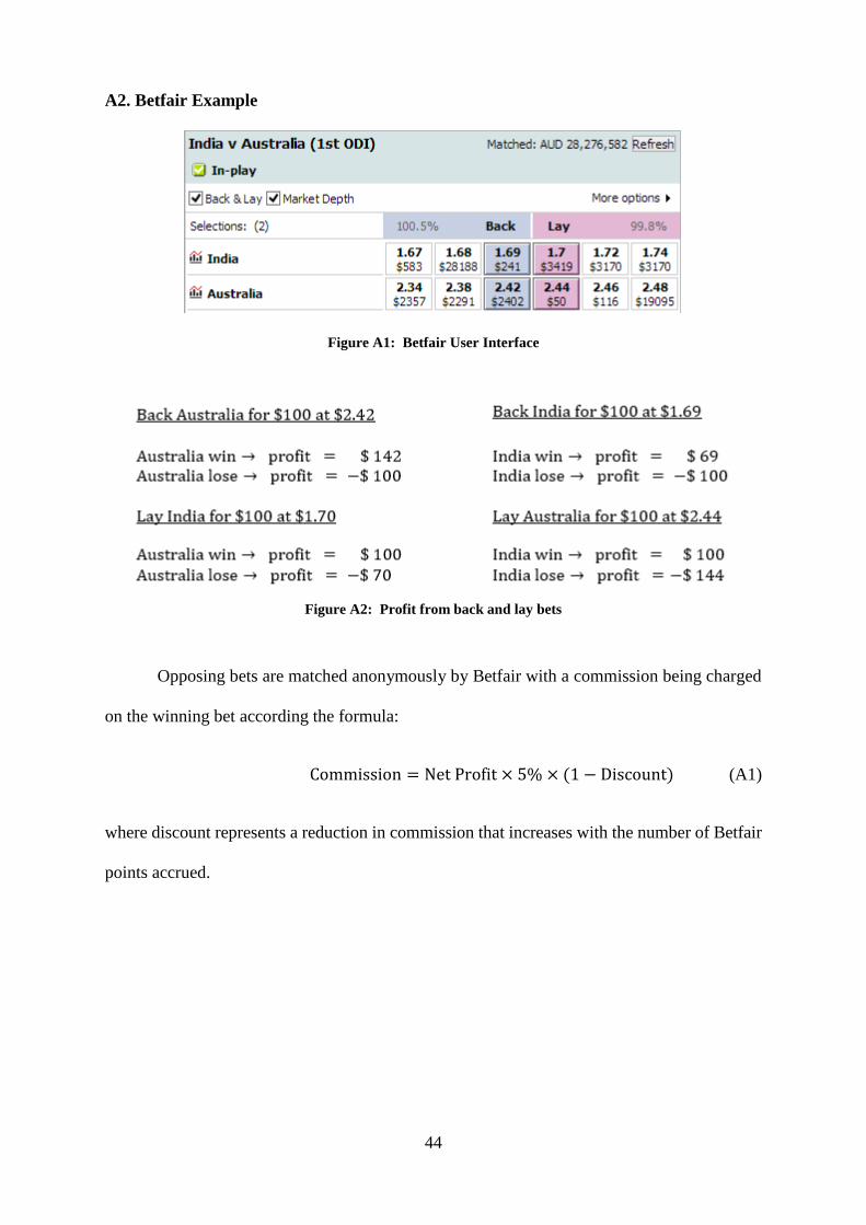
44

A2. Betfair Example

Figure A1: Betfair User Interface

Figure A2: Profit from back and lay bets

Opposing bets are matched anonymously by Betfair with a commission being charged

on the winning bet according the formula:

Commission = Net Profit × 5% × (1 − Discount) (A1)

where discount represents a reduction in commission that increases with the number of Betfair

points accrued.