Electronic copy available at: http://ssrn.com/abstract=1594116Electronic copy available at: http://ssrn.com/abstract=1594116Electronic copy available at: http://ssrn.com/abstract=1594116

WORKING PAPER SERIES

Center for Entrepreneurial and

Financial Studies

Working Paper No. 2010-3

Simulation-based valuation of project finance - Does model complexity

really matter?

FLORIAN WEBER

THOMAS SCHMID

MATTHÄUS PIETZ

CHRISTOPH KASERER

Electronic copy available at: http://ssrn.com/abstract=1594116Electronic copy available at: http://ssrn.com/abstract=1594116Electronic copy available at: http://ssrn.com/abstract=1594116

Simulation-based valuation of project finance - Does model

complexity really matter?

Florian Weber*

Thomas Schmid*

Matthäus Pietz*

Christoph Kaserer*

First version: January 2010

This version: April 2010

* Center for Entrepreneurial and Financial Studies (CEFS) and Department for Financial Management and Capital Markets,

TUM Business School, Technische Universität München, Arcisstr. 21, 80333 Munich, Germany

Corresponding author:

Florian Weber

Center for Entrepreneurial and Financial Studies (CEFS) and Department for Financial Management and Capital Markets,

TUM Business School, Technische Universität München, Arcisstr. 21, 80333 Munich, Germany

Phone: +498928925479 | Fax: +498928925488 | Email: florian.weber@wi.tum.de

Electronic copy available at: http://ssrn.com/abstract=1594116

Simulation-based valuation of project finance - Does model

complexity really matter?

Abstract

This paper analyzes the impact of model complexity on the net present value distribution and the expected default probability of equity investments in project finance. Model complexity is analyzed along two dimensions: simulation complexity and forecast complexity. We aim to identify model elements which are crucial for the valuation of project finance in practice.

First, we present a simulation-based project finance valuation model. Second, we vary several model aspects in order to analyze their impact on the valuation result. For forecast complexity, we apply different volatility and correlation forecasting techniques, e.g. correlation forecasts based on historical values and on a dynamic conditional correlation (DCC) model. Regarding simulation complexity, the number of Monte Carlo iterations, the equity valuation method, and the time resolution are varied.

We find that the applied volatility forecasting models have a strong influence on the expected net present value distribution and on the probability of default. In contrast, correlation forecasting models play a minor role. Time resolution and equity valuation are both crucial when specifying a valuation model for project finance. For the number of Monte Carlo iterations, we demonstrate that 100,000 iterations are sufficient to obtain reliable results.

Keywords: Project Finance, Investment Valuation, Stochastic Modeling, Monte Carlo Simulation, Forecasting, Model

Complexity

JEL classification: C63, Q40

Acknowledgments: Financial support from the TUM International Graduate School of Science and Engineering (IGSSE),

sponsored by Excellence Initiative of the German Federal and State governments, is gratefully acknowledged.

  3

1. Introduction

Modigliani and Miller’s (1958) seminal paper, showing that the financing decisions

made by companies are irrelevant for their market value, can be considered the origin of five

decades of research on financing decisions. However, the Modigliani-Miller theory builds on

the assumption of perfect and complete capital markets with rational investors. Since this is

rarely fulfilled in reality, financing decisions do affect the value of a firm, and are, therefore,

of huge importance. Among the numerous financing methods which have emerged over the

last decades, one method has started to gain increasing attention in the last years: project

finance. Finnerty (2007) defines project finance as “the raising of funds on a limited recourse

or non-recourse basis to finance an economically separable capital investment project in

which the providers of the funds look primarily at the cash flow from the project as the source

of funds to service their loans and provide the return of and a return on their equity invested in

the project.” One key element of project finance expressed in this definition and essential to

this paper is that debt and equity providers are primarily dependent on the project’s cash flow.

Hence, it is important to estimate the project’s future cash flows as accurate as possible in

order to quantify both, the probability of default (relevant for equity and debt providers), and

the expected profitability (only relevant for equity providers).

Starting with the successful financing of the North Sea oil field explorations in the

1970s, project finance became the state-of-the-art financing method for large-scale

investments (Kleimeier and Meggison 2001). Since then, project finance grew considerably

over the ensuing decades: from less than $10 billion per year in the late 1980s, to almost $328

billion in 2006 (Esty and Sesia 2007). Currently, over 50% of investments with capital

expenditures exceeding $500 million are project financed in the U.S. (Esty 2004). The most

prominent examples of project financed investments in recent years include the $4 billion

Chad-Cameroon pipeline and the $6 billion Iridium global satellite telecommunication system

(Esty and Sesia 2007).

Considering its importance in practice, the academic literature on project finance is

surprisingly sparse with only few relevant papers having been published in recent years. Most

of these papers focus on qualitative, organizational or legal aspects of project finance.1 To our

                                                            

1 See, for example, Chemmanur (1996), Esty and Megginson (2001), Esty and Megginson (2003) and Kleimeier and Megginson (2001). See also Esty (2004) for a comprehensive overview on research in project finance.

  4

best knowledge, only two papers, published by Esty (1999) and Gatti et al. (2007), highlight

the issue of cash flow modeling in the context of project finance. Esty (1999) discusses

methods to improve the valuation of project finance from an equity provider’s point of view.

To achieve this, he proposes both advanced discounting methods and valuation techniques.

However, besides discussing important elements for valuation, he does not present a self-

contained model which enables equity providers to calculate either the profitability of their

investments or the expected probability of a project default. Gatti et al. (2007) develop a

model to estimate the value-at-risk of project financed investments based on Monte Carlo

simulation. They solely focus on debt providers and ignore the equity providers’ point of

view.

In this paper we analyze the expected net present value (NPV) distribution and the

probability of default by Monte Carlo simulation. The question is whether complex valuation

techniques affect these substantially or whether simple models with less implementation

effort are sufficient enough for valuation purposes. In order to clarify this issue, we develop a

Monte Carlo simulation based cash flow valuation model, which we call project finance

valuation tool or PFVT in this paper. In the PFVT we combine stochastic cash flow modeling

and time-series forecasting techniques. We analyze if model complexity matters by a case

study on an equity investment in a coal power plant. We vary the complexity of the

simulation parameters, e.g. the number of iterations of the Monte Carlos simulation or the

simulation’s time resolution, and forecast models, e.g. evolving from the case of no

correlations to correlations obtained from the Dynamic Conditional Correlation (DCC) model

proposed by Engle and Sheppard (2001). A detailed overview of the variations applied is

provided in section 3.

We contribute to the existing literature along two dimensions. To the best of our

knowledge, we are the first to present and describe a self-contained simulation-based

valuation tool for project finance. Additionally, we address the issue of model complexity and

its effect on the valuation results. This should be of particular interest for practitioners, who

have to decide whether an increase in the valuation accuracy or a lower implementation effort

of the applied valuation tools is more important when valuating real-life investments.

This paper is organized as follows: Section 2 provides an overview of project finance

valuation, including a description of the PFVT. In section 3 the case study is presented and

  5

valuation results obtained by models with different levels of complexity are reported. In

section 4, we conclude our results and discuss avenues for further research.

2. Project Finance Valuation

2.1 General Remarks

Today, the discounted cash flow (DCF) analysis is the most common concept applied

in valuation. In the context of investment valuation, the DCF can be used to value equity

investments in two ways: Indirectly by discounting the free cash flow to the firm (FCFF) with

help of the weighted average cost of capital (WACC) and subtracting the debt value (plus

cash) afterwards, or directly by discounting the free cash flow to equity (FCFE) using the cost

of equity. Two types of issues for the calculation of the net present value (NPV) arise at this

point: First, it is important to account for the uncertainty of the future cash flow. Second, the

determination of the risk-adjusted cost of capital is not straightforward. Following Vose

(2000), the main solutions which allow the consideration of the future cash flows' uncertainty

in investment projects are either a deterministic scenario-based modeling approach or the

application of Monte Carlo simulation. In a deterministic model, the analysis concentrates on

different scenarios with each scenario representing a single-point estimate. However, this

technique has the drawback that not every possible future state is taken into consideration.

Monte Carlo simulation overcomes this drawback by random sampling from several

probability distribution functions to generate a joint probability distribution function. For this,

it is necessary to forecast the future probability distribution function of all factors which

influence the cash flow. Although this technique is rather complex, it is the only appropriate

for a detailed analysis of a project as other techniques use simplifications which may bias the

results substantially.

The estimation of the cost of equity is a crucial task as well. In general, the cost of

equity is estimated with the Capital Asset Pricing Model (CAPM) or the Arbitrage Pricing

Theory (APT). In standard valuation theory, DCF analysis is mainly applied to industry

companies with rather stable capital structures. Therefore, a single, constant discount rate is

used. This technique is not appropriate for the valuation of project financed investments, since

they are characterized by a limited runtime and time-varying capital structures. A

recommended solution is the assumption of a target capital structure which allows the

calculation of a discount rate (Ehrhardt 1994, Copeland et al. 1996 and Finnerty 2007). This

  6

technique may lead to a miscalculation of the project’s cost of equity since its cost of equity

depends on the project’s time-varying capital structure (Esty 1999).2 Damodaran (1994) and

Grinblatt and Titman (2001) argue that only the application of different discount rates for

every year based on the actual capital structure produces unbiased costs of equity. We include

this technique in our model by determining the cost of equity each time the cash flow is

calculated. Furthermore, Esty (1999) argues that it is crucial to calculate the cost of equity

based on market values for debt and equity instead of their book values. This leads to a

circularity problem: The market value of equity, which is calculated as the book value of

equity plus the NPV, cannot be calculated since the cost of equity is necessary for that. A

possible solution, originally proposed by Richard Ruback and first applied to project finance

valuation by Esty (1999), is the so called quasi-market valuation (QMV).3 According to this

method, the market value of equity at the end of year 0 equals the initial book value of equity

plus the expected NPV of the project. We include this technique in our model since QMV is

the best realizable method to avoid biased estimates of the cost of equity.

2.2 Cash flow modeling

2.2.1 Monte Carlo simulation

Hess and Quigley (1963) were the first to apply Monte Carlo simulation in finance.4

Hertz (1964a,b) proposed that applying simulation techniques instead of single-point

estimates of future income and expenses is superior when appraising capital expenditure

proposals under conditions of uncertainty. He argues that potential risks are more clearly

identified, and the expected return is more accurately measured. Smith (1994) outlines how

simulations may assist managers in choosing among different potential investment projects.

Spinney and Watkins (1996) apply Monte Carlo simulation as a technique for integrated

resource planning at electric utilities. They find that Monte Carlo simulation offers

advantages over more commonly used methods for analyzing the relative merits and risks

                                                            

2 This miss-estimation of the cost of equity also distorts the calculation of the WACC. 3 The QMV is based on three main assumptions: (i) the CAPM holds, (ii) the market value of debt is equal to the book value of debt, and (iii) the market is efficient. 4 The first documented application of Monte Carlo methods was performed by von Neumann, Ulam and Fermi for nuclear reaction studies in the Los Alamos National Laboratory (Metropolis and Ulam 1949, Metropolis 1987). Hammersley and Handscomp (1964), followed by Glynn and Witt (1992), were the first to discuss the relationship between accuracy and computational complexity of Monte Carlo simulations. Since Monte Carlo simulation is computationally intensive and, hence, reliant on fast calculating machines, its application for the solution of scientific problems rose as the costs for powerful processor decreased over the last two decades.

  7

embodied in typical electrical power resource decisions, particularly those involving large

capital commitments. More recently, Kwak and Ingall (2007) discuss Monte Carlo simulation

for project management and conclude that it is a powerful tool to incorporate uncertainty and

risk in project plans.

2.2.2 Forecasts

The determination of future values of the factors influencing a project financing’s cash

flow is critical for its valuation. Since this development is a priori unknown, forecasting

models have to be applied to obtain estimates for the future mean values. However, not only

the future mean values of the influencing factors are of interest. To perform consistent Monte

Carlo simulations, the future variances of the factors and correlation structures between the

factors have to be estimated as well. Since literature on forecasting is numerous, a complete

overview of all available models and methods is beyond the scope of this paper.5 For mean or

price forecasts, we apply (i) simple random walk with and without drift (Fama 1965), (ii)

autoregressive moving average (ARMA) (Box and Jenkins 1970), and (iii) mean reversion

forecasts (Vasicek 1977). To estimate future variance and correlation structures, we apply (i)

historical standard deviation and correlation, (ii) GARCH-type models6 as proposed by

Bollerslev (1986), and (iii) Dynamic Conditional Correlation (DCC) models as proposed by

Engle and Sheppard (2001).

2.2.3 Project Finance Valuation Tool (PFVT)

The PFVT is a tool which enables an investor to calculate the expected NPV

distribution of his equity stake in a project financed investment as well as the project’s

expected default probability. To achieve this, the tool relies on the direct valuation method,

implicating that no accounting issues are taken into consideration. The PFVT is programmed

in MATLAB, a programming language often used for numerical applications.

First, the user has to specify all relevant parameters for the project’s cash flow. For

these factors, we have implemented several forecast models for mean values, volatility and

correlation. Historical time series for various financial assets are included in the PFVT and

                                                            

5 See, for example, Geman (2005) or Weron (2006) for a detailed overview on forecasting models. 6 The GARCH derivatives GJR-GARCH (as proposed by Glosten et al. 1993) and E-GARCH (as proposed by Nelson 1991) are included in model as well.

  8

can be updated on request. These time series can be used for the parameter estimation of the

forecast models. However, the parameters can also be specified manually . Beneath input and

output factors with historical time series, the PFVT allows the manual input of non-financial

factors as well. For this, the user may choose between different distributions, e.g. rectangular

or triangular distribution with or without drift. This enables the consideration of non-Gaussian

distributed factors. In a second step, the user has to define project specifics, which include, for

example, the lifespan of the project, the financing structure of the project, or the input-output

relationship. Additionally, some parameters for the simulation must be specified, like the

desired frequency of cash flow distributions reported, the time-resolution, which determines

how often the cash flow is analyzed, or the number of iterations. The duration of the

simulation procedure depends significantly on this input parameter (c. section 3.4.1. for a

detailed analysis).

The user is able to define all of the above mentioned parameters inside a spreadsheet

file.7 The results, which are generated in MATLAB, are stored in an output file and can be

exported to a spreadsheet file. This file contains, among others, the following information: (i)

the distribution of the project’s NPV, (ii) the expected cumulated default probability, (iii) for

each cash flow time point the free cash flow to equity distribution, default probability, cash

flows at risk, coverage ratios and leverage ratios, and (iv) the underlying forecasts of the

individual factors.

3. Case Study

3.1 Project Description

The PFVT is applied to calculate the profitability of a project financed coal power

plant. As mentioned beforehand, we take the equity provider’s point of view. A power plant is

chosen based on two main considerations: First, investments in the energy sector are

characterized by high initial capital expenditures, often reaching the range of billions. Hence,

it is not surprising that project finance is the most common financing method in this sector.

                                                            

7 The spreadsheet file serves as a graphical front-end, but the computation is performed in MATLAB.

  9

Second, data availability for power plants is excellent since we can access data from a

research cluster focusing on power plants.8

The rationale behind performing this case study is twofold. First, we want to illustrate

the capabilities of the PFVT by analyzing a realistic project. Second, and most important, we

want to explore whether model complexity has an impact on the obtained results. As a

detailed consideration of all aspects of a real-life power plant project is beyond the scope of

this paper, we apply several simplifications to ease the specification of the project.9 Since we

are not primarily interested in the results for this certain project, but in the effect of model

complexity, we expect these simplifications not to bias our results. The major (technical)

assumptions concerning the power plant project are summarized in section 3.2.

We assume that investors taking an equity stake in project finance typically have a

limited investment horizon of three to seven years.10 By contrast, power plant projects have a

runtime of 20 years and more. As a consequence, an equity investor must sell his stake in the

project during its runtime. In order to do this, it is crucial for the investor to be able to

determine the value of his stake at any point of time. The PFVT can simulate the project over

its whole runtime. A simulation over such a long period of time is not meaningful from an

economic point of view. To solve this issue, we model the project over a horizon of 5 years

and assume that the whole project is sold to another investor afterwards. The selling price is

calculated with the help of a valuation technique based on cash flow multiples.

3.2 Model calibration

We assume that the coal power plant’s construction takes place in one point of time,

and that it is operated as a base load power plant. After the initial capital expenditure, we

identify three main categories of relevant costs for the power plant project: (i) fixed costs: e.g.

salaries, insurances, (ii) variable costs: e.g. chemicals, (iii) fuel costs: costs for coal, (iv) and

costs for emission rights. Furthermore, the power plant generates revenues which are

dependent on the amount of electricity produced and the electricity price. The computation of

the amount of electricity produced is not straightforward since several factors have to be taken                                                             

8 We thank the members of TUM International Graduate School of Science and Engineering for their support and the in-depth discussions. 9 These assumptions are made due to simplification matters and are not necessary for the PFVT, since the tool can handle complex project structures. 10 This assumption is based on discussions with project finance investors.

  10

into consideration: (i) capacity, (ii) load factor, (iii) operating time, and (iv) efficiency. To

ease matters, we assume that there is no technical improvement over the project’s runtime

meaning the efficiency remains constant. The most important influencing factors on the

project’s cash flow are the price of electricity, the fuel costs (coal input per MWh of

electricity output), and the costs for emissions rights (EUA costs per MWh of electricity

output) because they largely determine the profitability of the power plant.

An initial investment of €1 billion is assumed. The financial structure in our case study

corresponds to a typical project financed power plant. The debt-to-equity ratio at the

beginning of the project is 2 and the debt has a maturity of 20 years. Furthermore, we assume

that one third of the debt is provided in U.S. Dollar and two thirds are provided in Euro. The

runtime of the power plant is estimated to be 40 years, with total depreciation taking place

over 20 years. The whole free cash flow to equity is immediately distributed among the equity

providers. An event of default occurs in general when the free cash flow to equity becomes

negative, implying that equity providers must re-invest cash in the project. Since this

assumption is very restrictive and also not meaningful from an economic point of view, it is

relaxed by assuming that equity providers have the obligation to re-invest money in the

project until a threshold of one third of their initial investments. After that, every negative free

cash flow to equity leads to an event of default of the project. As already mentioned in section

2, the capital structure of the project and its cost of equity is permanently recalculated and

adjusted during the simulated period of the project.11

Regarding the technical parameters of the power plant, an electricity generation

capacity of 1000 MW, a load factor of 69% and an availability of 84% are presumed.

Operation and maintenance costs are 5% of the revenue and, in addition, €1 for every

generated MWh. Fixed costs are assumed to have a magnitude of €5 million per year,

including labor costs. For the relation between electricity output and fuel input we assume

that 0.978 emission rights are necessary for every generated MWh of electricity. Additionally,

36% thermal efficiency is assumed for the generation process.

The starting point of our analysis is May 2009. As mentioned above, we model the

first 5 years of the project’s runtime. After that, the project is sold for a price based on a cash

                                                            

11 A theoretical reasoning for this approach can be found in Damodaran (1994) and Grinblatt and Titman (1998).

  11

flow multiple valuation approach. As common for power plant valuations, we calculate its

value as two times the average of its last three annualized free cash flows to equity.

The following forecast models are used for the different influencing factors: For the

electricity price, the emission rights, the interest rates and the U.S. Dollar / Euro exchange

rate we apply an ARMA(1,1) model. For the coal price an ARMA(2,2) model is used.12 The

power plant is assumed to operate 24 hours, 7 days a week (common for base load power

plants). This allows us to forecast electricity prices without consideration of their

peculiarities, especially their extreme intra-day and intra-week variation. We use the

European Energy Exchange (EEX) electricity (baseload day-ahead) spot price as our

reference price for electricity. All price forecasts are based on these data.

3.3 Model complexity

The effect of the model complexity on the simulation results is the key element of this

paper. In the following, we divide model complexity in two components: (i) the complexity of

the simulation procedure and (ii) the complexity of the forecast models. The complexity of

the simulation procedure is defined along three dimensions, the number of iterations, the

time-resolution (which defines how often the cash flow is analyzed) and the valuation method

for equity. In order to explore their effects on the simulation results, we vary these three

components in several dimensions. For forecast complexity, we vary the volatility and the

correlation forecast models. For volatility forecasts, we use (i) historical volatility and

forecasts obtained from a (ii) GARCH(1,1), an (iii) E-GARCH as well as a (iv) GJR-model.

For correlations, we apply (i) no correlations, (ii) historical correlations and (iii) correlations

obtained from a DCC-GARCH model. Figure 1 summarizes the different variations of the

model complexity.

- Insert figure 1 around here -

In the following sections, we present the simulation results of the PFVT and analyze

the effect of model complexity on the NPV distribution and the (cumulative) default

probability of the project.

                                                            

12 A thorough discussion of different mean models can be found in Geman (2005) or Weron (2006).

  12

3.4 Results

The simulation results are presented in two sub-sections. We describe the effect of the

simulation complexity on the results in the first sub-section, and the effect of forecast

complexity in the second. We analyze the project’s NPV cumulative distribution function

(CDF) and – if meaningful – its expected cumulative default probability (ECDP). The CDF

graphs display the NPV on the x-axis and the cumulative probability on the y-axis. The ECDP

graphs show the time elapsed since project start on the x-axis and the cumulative expected

default on the y-axis.

We define a reference model which will be applied in all simulations. In each step,

one parameter will be changed. Our base case model has the following properties: (i) price

forecasts are obtained by ARMA-models13, (ii) volatilities are forecasted with the help of a

GARCH (1,1) model, (iii) future correlations are assumed to be equal to historical

correlations, (iv) the model’s time resolution is weekly, (v) the calculation of the equity’s

market value is based on the QMV-method, and (vi) the number of iterations is 100,000.

3.4.1 Simulation complexity

The number of iterations is the first parameter to analyze. It is expected that an

increase in this parameter leads to a smoother distribution function of the NPV.

- Insert figure 2a around here -

As expected, the level of the distribution function remains (largely) unchanged. Figure

2a presents the distribution function of simulations with different numbers of iterations. We

simulate the project with 1,000, 10,000, 100,000, and 500,000 iterations. As expected, the

number of iterations has no significant effect on the overall level since there is no systematic

shift in the cumulative distribution function. However, for 1,000 and 10,000 iterations, the

function is rather unsteady, as shown in the enlargement of figure 2a. As a consequence, the

expected NPV may be over- or underestimated, depending on whether the function is above

or below its “true” value at a certain point. The application of at least 100,000 of iterations

seems to be favorable. The step from 100,000 to 500,000 iterations does not increase the

smoothness of the function significantly. We recommend using at least 100,000 iterations for                                                             

13 We do not vary the price forecast models since their impact on the simulation results is obvious.

  13

a simulation to obtain smooth distribution functions. The same effects can be observed for the

ECDP, which is reported in figure 2b.

- Insert figure 2b around here -

The drawback of an increased number of iterations is that the computation time rises

significantly. As presented in figure 3, the computation time on our system, a commercially

available high-end personal computer, rises from 2 minutes for 1,000 iterations to 270

minutes for 500,000 iterations. Therefore, it is necessary to weight the advances of an

increased number of iterations, a smoother distribution function, against its drawback in terms

of longer computation time. As mentioned beforehand, an increase from 100,000 to 500,000

iterations does not lead to a strong improvement in smoothness, but to a five times higher

computation time. Below 100,000 iterations, the distribution function is very rocky and not

satisfying. As a consequence, the above proposed 100,000 iterations seem, from this point-of-

view, to be a good compromise between distributions smoothness and computation time.

- Insert figure 3 around here -

Next, we analyze the impact of the applied equity valuation method on the simulation

results. Figure 4 presents the two methods included in the PFVT, equity valuation based on

QMV, and on book values.

- Insert figure 4 around here -

We find that the cumulative distribution function differs for the two methods. The

NPV distribution is narrower with less extreme values for the equity valuation based on book

values compared to the QMV. The rationale behind this is that the application of equity book

values leads to biased estimates of the cost of equity, since they are not linked to the success

of the project. In reality, the costs of equity depend on the successfulness and, hence, on the

risk of a project. Since book value estimation does not account for that, it overestimates the

costs of equity for very successful projects and underestimates them for unsuccessful projects.

The QMV links the costs of equity to the profitability of a project in order to avoid this

misjudgment. This estimation leads on the one hand to more extremely high NPV estimates

(because the discount rate for successful projects is smaller) and on the other hand to more

extremely low NPV values (because the discount rate for unsuccessful projects is higher).

  14

This is what can be seen in the cumulative distribution function. The ECDP of the project is

not affected by the equity valuation method. Consequently, we do not report this figure here.

Another crucial parameter of the simulation is the time resolution. The time resolution

defines how often the project’s cash flow is analyzed. For example, a weekly time resolution

means that the cash flow of the project is computed and analyzed each week during the

simulation phase of the project. We analyze the impact of a weekly, monthly and a yearly

time resolution. Figure 5a presents the impact of the time resolution on the simulation results.

- Insert figure 5a around here -

As can be seen, a higher time resolution leads to a broader NPV distribution and to

more extreme positive and negative events. The higher frequency of small (negative) NPV

values is not surprising, since a higher time resolution is accomplished by more default

events, as presented in figure 5b.

- Insert figure 5b around here -

Since the cash flow is analyzed more often with, for example, weekly resolution

compared to yearly resolution, a stream of negative cash flows over several weeks may lead

to a project default. These events of default do not necessarily happen with yearly resolution,

since a stream of negative cash flows may be followed by more positive cash flows which

compensate the prior losses. However, on a weekly resolution the project would have been

defaulted with no possibility of recovering. The explanation of the higher frequency of large

NPV values is more complicated. One aspect which has to be taken into consideration is the

effect of discounting, since a higher time resolution leads to smaller discounting steps. As a

result, large positive values in the future are discounted with a lower average discounting rate

for high-time frequencies, leading to higher NPV values today.

3.4.2 Forecast complexity

The first issue to address within the area of forecast complexity is how future

volatilities are predicted. The PFVT is able to apply either historical volatility values as

forecasts for future volatility or to compute those estimates based on different GARCH type

models. Beneath the GARCH(1,1) model, we also apply the more advanced E-GARCH and

GJR-model. An issue worth mentioning is that forecasts based on GARCH models converge

  15

to forecasts based on historical values after a certain span of time. The impact of volatility

forecasts on the simulation results is presented in figure 6a.

- Insert figure 6a around here –

As can be seen, the results depend heavily on the applied volatility forecast model.

The E-GARCH model leads to a much narrower NPV distribution compared to the other

models. The broadest NPV distribution is obtained with the GJR-GARCH model. When

analyzing the project’s ECDP, which is reported in figure 6b, the same effects can be found.

- Insert figure 6b around here –

Especially the E-GARCH model is noticeable since it leads to a much lower default

probability. The gap between the default probability calculated by the E-GARCH and the

GJR-GARCH model is about 10% over the whole runtime of the project. We cannot judge

which model is the best model since we do not know the “real” cumulative default

probability. However, our results suggest the choice of the volatility forecast model is

extremely crucial for the simulation results. Hence, it is very important to figure out which

volatility forecast model is best suited for each factor when valuing a project in practice. The

substantial impact of this choice can be seen from the prior two figures. Recent academic

work by Bowden and Payne (2008), and Chan and Gray (2006) propose that E-GARCH is the

best volatility model for electricity prices. Hence, it could be argued that its application

should be favored over alternative models.

In a further step, we investigate the influence of the correlation forecast model. The

PFVT can compute future correlations in three different ways: (i) it assumes that the

correlation between all factors is zero in the future (ii) historical correlations are used as

forecasts for future correlations (iii) estimates from a DCC model are applied as predictors for

correlations. The first method, which assumes zero correlations, has to be interpreted with

caution since fundamental economic relationships may be neglected. For example, if a project

is simulated whose cash flow depends on gas and oil prices, the assumption of no correlation

is clearly misleading, since gas and oil prices are highly correlated due to linking mechanism

between them. However, we integrated that possibility to investigate if the assumption of no

  16

correlation has a significant impact on the results of our case study.14 Figure 7a presents the

cumulative NPV distribution function for these three different correlation forecasts.

- Insert figure 7a around here –

As can be seen, the choice of the correlation forecast has a limited impact on the

simulation results, especially compared to the choice of the volatility model. The simulated

NPV distributions are relatively equal for all three correlation forecast methods. The same is

true for the ECDP, which is reported in figure 7b.

- Insert figure 7b around here –

To summarize, our results suggest that correlation forecasts based on a DCC model do

not significantly improve the result compared to the application of historical correlations.

Taking into consideration that the DCC model is rather complicated to implement in a

valuation model, we suggest using historical correlations, which are easier to handle.

4. Conclusion

This paper aims to analyze, whether model complexity matters for the valuation of

project finance based on Monte Carlo simulation. We analyze the effect on the net present

value (NPV) distributions and the estimated default probabilities. For this purpose, we use a

newly developed Monte Carlo simulation based cash flow valuation model and apply it to a

power plant in the context of a case study. We distinguish between two dimensions of model

complexity: (i) the complexity of the simulation procedure and (ii) the complexity of the

forecast models. We summarize our results as follows: Regarding the simulation parameters,

we find that considering the trade-off between result adequacy and computation time, a

number of 100,000 iterations seems to be the optimal choice. Furthermore, the quasi-market

valuation method should be used when valuing projects. If this is not the case the project’s

cost of capital is either over- or understated, resulting in biased valuation results. Analyzing

the effect of the time resolution, we find that it is significant on the calculation of the default

probability. When using the typical text book assumption that the cash flow is received at the

end of a period, then the time resolution has also an impact on the NPV distribution. This is

due to the discounting of the individual cash flows. When analyzing the effect of the forecast                                                             

14 As for GARCH based volatility forecasts, correlation forecasts based on the DCC model converge to forecasts based on historical values after a certain time.

  17

models, we find that the selected volatility forecast model significantly affects the simulation

results. The effect of the correlation forecast model seems to be less pronounced. To

summarize, we can show that model complexity is important in the context of project finance

valuation. However, there are model elements that are extremely crucial, while other seem to

be less important.

Based on our results, future research on this topic seems to be promising. The main

avenue for further research is the question if our results hold true in a non-energy project

finance context. Project financed investments in other industries, e.g. telecommunication or

infrastructure should be used to test issues of model complexity. However, reliable data for

those industries is hard to obtain, since little information is publicly available. Furthermore,

there are promising extensions that could be included in the PFVT, like more complex

valuation methods (e.g. real options) and more complex forecasting techniques (e.g. BEKK-

GARCH).

  18

References

Bollerslev, T. (1986): Generalized Autoregressive Conditional Heteroskedasticity, in: Journal of Econometrics 31, 307-327.

Box, G.E.P and Jenkins, G.M. (1970): Time Series Analysis - Forecasting and Control. John Wiley, San Francisco.

Chemmanur, T.J. and John, K. (1996): Optimal Incorporation, Structure of Debt Contracts, and Limited-Recourse Project Financing, in: Journal of Financial Intermediation 5, 372-408.

Copeland, T., Koller, T. and Murrin J. (1996): Valuation: Measuring and Managing the Value of Companies, Second Edition, John Wiley, New York, 1996.

Damodaran, A. (1994): Damodaran on Valuation: Security Analysis for Investment and Corporate Finance, John Wiley, New York, 1994.

Ehrhardt, M.C. (1994): The Search for Value: Measuring the Company's Cost of Capital, Harvard Business School Press, Boston, 1994.

Engle, R.F. and Sheppard, K. (2001): Theoretical and Empirical properties of Dynamic Conditional Correlation Multivariate GARCH, in: NBER Working Papers 8554.

Esty, B.C. (1999): Improved techniques for valuing large-scale projects, in: The Journal of Project Finance 5, 9-25.

Esty, B.C. and Megginson, W.L. (2001): Legal Risk as a Determinant of Syndicate Structure in the Project Finance Loan Market, in: Working Paper, Harvard Business School.

Esty, B.C. and Megginson, W.L. (2003): Creditor Rights, Enforcement, and Debt Ownership Structure: Evidence from the Global Syndicated Market, in: Journal of Financial and Quantitative Analysis 38, 37-59.

Esty, B.C. (2004): Why Study Large Projects? An Introduction to Research on Project Finance, in: European Financial Management 10, 213-224.

Esty, B.C and Sesia, A. (2007): Overview of Project Finance and Infrastructure Finance, in: Harvard Business School Cases.

Fama, E. F. (1965): Random Walks In Stock Market Prices, in: Financial Analysts Journal 21, 55-59.

Finnerty, J. D. (2007): Project financing: asset-based financial engineering. John Wiley, New York, 2007.

  19

Gatti, S., Rigamonti, A., Saita, F. and Senati, M. (2007): Measuring Value-at-Risk in Project Finance Transactions, in: European Financial Management 13, 135-158.

Geman, H. (2005): Commodities and Commodity Derivatives: Modelling and Pricing for Agriculturals, Metals and Energy. John Wiley, New York, 2005.

Glosten, L. R., Jagannathan, R. and Runkle, D.E. (1993): On the Relation between the Expected Value and the Volatility of the Nominal Excess Return on Stocks, in: Journal of Finance 48, 1779-1801.

Glynn, P. W. and Witt, W. (1992): The Asymptotic Efficiency of Simulation Estimators, in: Operations Research 40, 505-520.

Grinblatt, M. and Titman, S. (2001): Financial Markets and Corporate Strategy. Second edition. Irwin McGraw-Hill, Boston, 2001.

Hammersley, J. M. and Handscomp, D. C. (1964): Monte Carlo Methos. Methuen, London, 1964.

Hertz, D. B. (1964a): Risk Analysis in Capital Investment, in: Harvard Business Review 42, 95-106.

Hertz, D. B. (1964b): Investment Policies That Pay Off, in: Harvard Business Review 46, 96-108.

Hess, S. W. and Quigley, H. A. (1963): Analysis of Risk in Investments Using Monte Carlo Techniques, in: Chemical Engineering Symposium Series 42: Statistical and Numerical Methods in Chemical Engineering, 55-71.

Kleimeier, S. and Megginson, W.L. (2001): An empirical analysis of limited recourse project finance, in: Working Paper, University of Oklahoma.

Kwak, Y. H. and Ingall, L. (2007): Exploring Monte Carlo Simulation Applications for Project Management, in: Risk Management 9, 44-57.

Metropolis, N. and Ulam, S. (1949): The Monte Carlo Method, in: Journal of the American Statistical Association 44, 335-341.

Metropolis, N. (1987): The beginning of the Monte Carlo method, in: Los Alamos Science, 125-130.

Modigliani, F. and Miller, M. (1958): The cost of capital, corporate finance and investment, in: American Economic Review 48, 655-669.

  20

Nelson, D. B. (1991): Conditional heteroskedasticity in asset returns: A new approach, in: Econometrica 59, 347-370.

Smith, D. (1994): Incorporating Risk into Capital Budgeting Decisions Using Simulation, in: Management Decision 32, 20-26.

Spinney, P. J. and Watkins, G. C. (1996): Monte Carlo simulation techniques and electric utility resource decisions, in: Energy Policy 24, 155-163.

Vasicek, O. (1977): An Equilibrium Characterisation of the Term Structure, in: Journal of Financial Economics 5, 177–188.

Vose, V. (2000): Risk Analysis: A Quantitative Guide. Second edition. John Wiley, New

York, 2000.

Weron, R. (2006): Modeling and Forecasting Electricity Loads and Prices: A Statistical

Approach. John Wiley, New York, 2006.

  21

Figure 1: Dimensions of model complexity

Model Complexity

Forecast Models Simulation Procedure

Level

Volatility

Correlation

NonHistorical

DCC

ARMA(1,1)

HistoricalGARCH

EGARCHGJR

Iterations

Resolution

Equity Value

DailyWeekly

Monthly

1000

Book ValueQMV

10000100000500000

  22

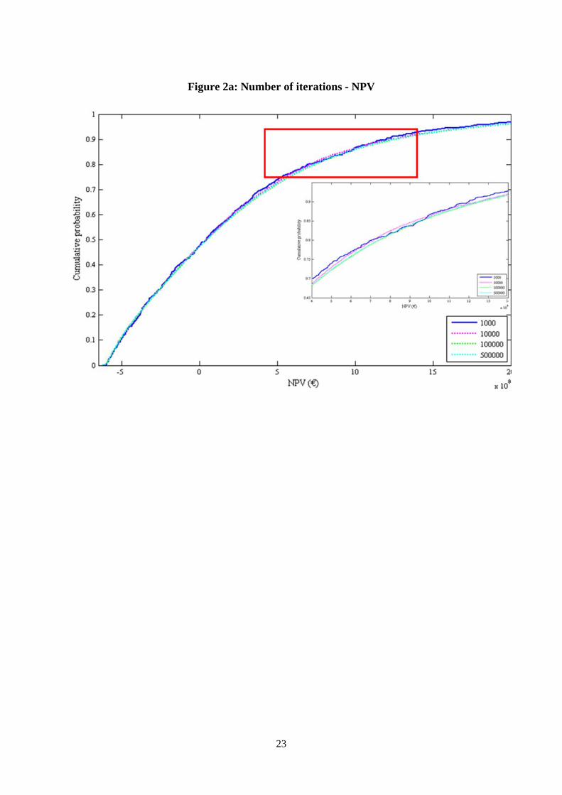
Figure 2a: Number of iterations - NPV

  23

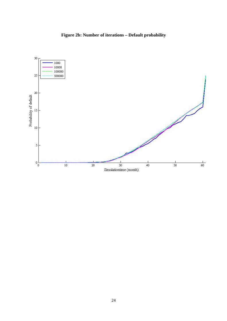
Figure 2b: Number of iterations – Default probability

  24

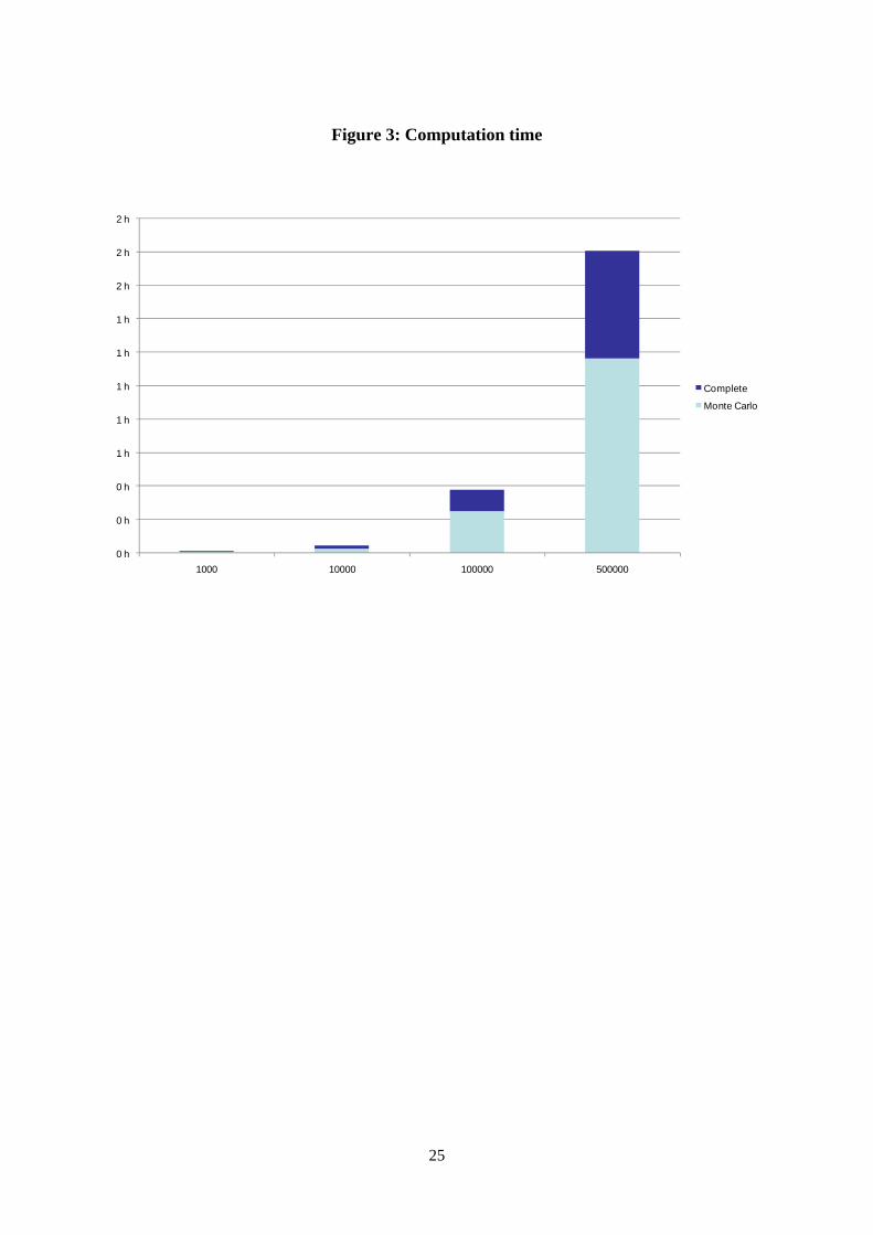
Figure 3: Computation time

0 h

0 h

0 h

1 h

1 h

1 h

1 h

1 h

2 h

2 h

2 h

1000 10000 100000 500000

Complete

Monte Carlo

  25

Figure 4: Equity valuation method - NPV

  26

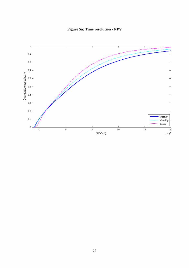
Figure 5a: Time resolution - NPV

  27

Figure 5b: Time resolution – Default probability

  28

Figure 6a: Volatility model - NPV

  29

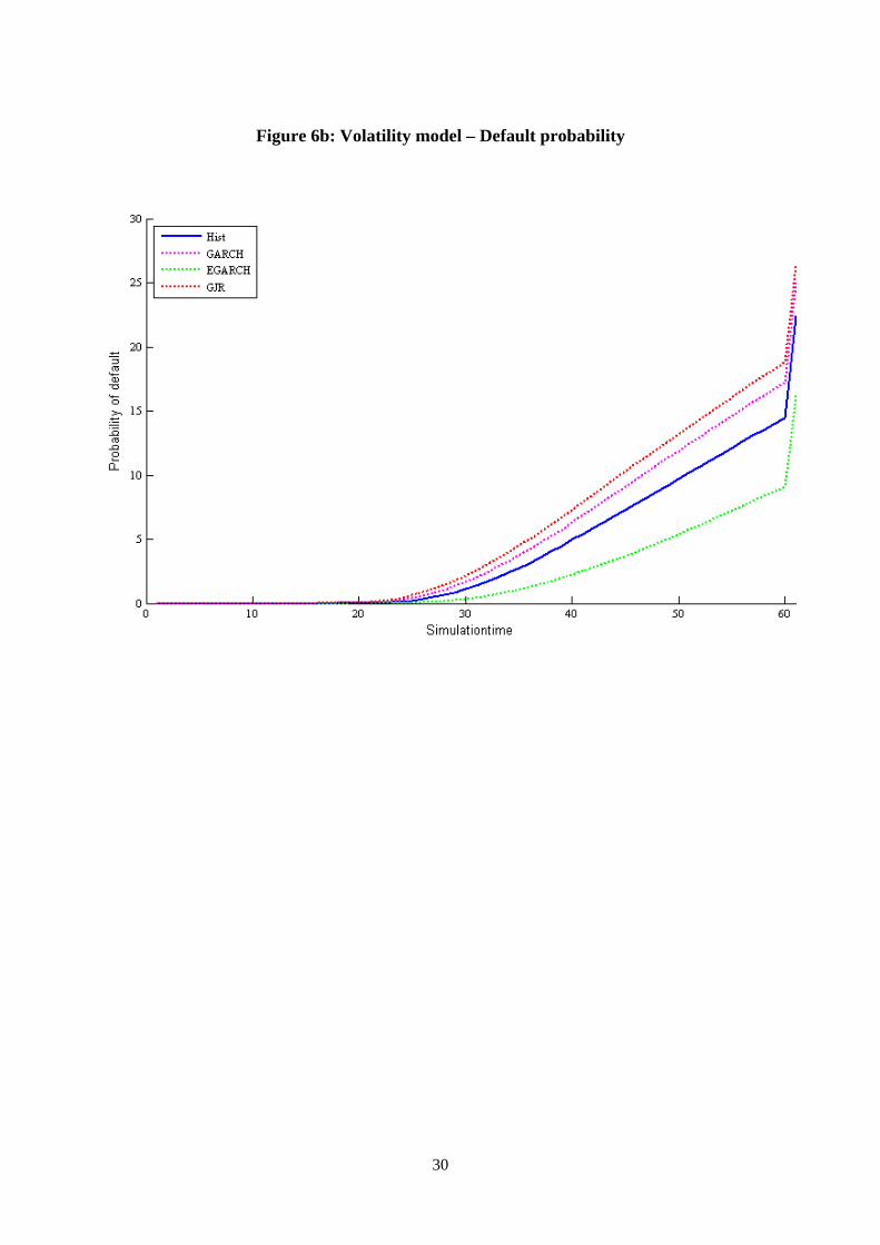
Figure 6b: Volatility model – Default probability

  30

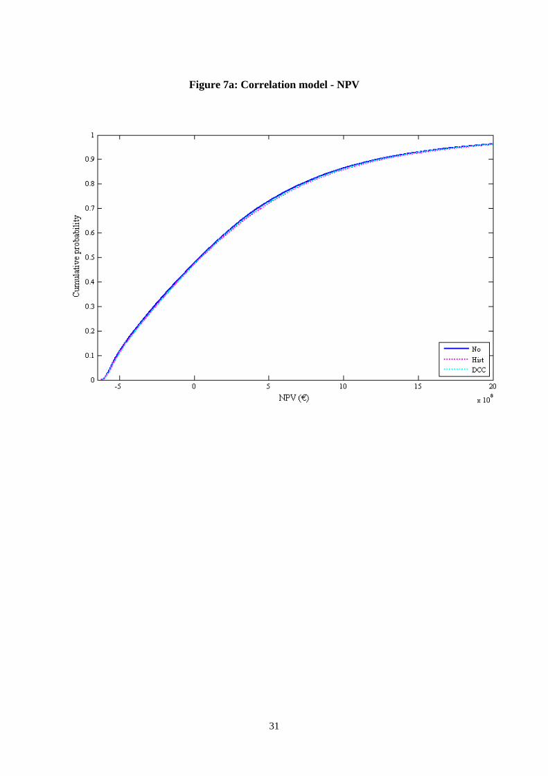
Figure 7a: Correlation model - NPV

  31

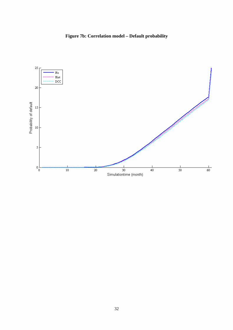
Figure 7b: Correlation model – Default probability

  32