word classes and part-of-speech tagging t...t 4 chapter 5. word classes and part-of-speech tagging...

DRAFT

Speech and Language Processing: An introduction to speech recognition, computationallinguistics and natural language processing. Daniel Jurafsky & James H. Martin.Copyright c© 2006, All rights reserved. Draft of July 30, 2007. Do not cite withoutpermission.

5WORD CLASSES ANDPART-OF-SPEECHTAGGING

Conjunction Junction, what’s your function?Bob Dorough,Schoolhouse Rock, 1973

A gnostic was seated before a grammarian. The grammariansaid, ‘A word must be one of three things: either it is a noun, averb, or a particle.’ The gnostic tore his robe and cried, “Alas!Twenty years of my life and striving and seeking have gone to thewinds, for I laboured greatly in the hope that there was anotherword outside of this. Now you have destroyed my hope.’ Thoughthe gnostic had already attained the word which was his purpose,he spoke thus in order to arouse the grammarian.

Rumi (1207–1273),The Discourses of Rumi, Translated by A. J. Arberry

Dionysius Thrax of Alexandria (c. 100 B.C.), or perhaps someone else (exact au-thorship being understandably difficult to be sure of with texts of this vintage), wrotea grammatical sketch of Greek (a “techne”) which summarized the linguistic knowl-edge of his day. This work is the direct source of an astonishing proportion of ourmodern linguistic vocabulary, including among many other words,syntax, diphthong,clitic, andanalogy. Also included are a description of eightparts-of-speech: noun,PARTSOFSPEECH

verb, pronoun, preposition, adverb, conjunction, participle, and article. Although ear-lier scholars (including Aristotle as well as the Stoics) had their own lists of parts-of-speech, it was Thrax’s set of eight which became the basis forpractically all subsequentpart-of-speech descriptions of Greek, Latin, and most European languages for the next2000 years.

Schoolhouse Rock was a popular series of 3-minute musical animated clips firstaired on television in 1973. The series was designed to inspire kids to learn multipli-cation tables, grammar, and basic science and history. The Grammar Rock sequence,for example, included songs about parts-of-speech, thus bringing these categories intothe realm of popular culture. As it happens, Grammar Rock wasremarkably tradi-tional in its grammatical notation, including exactly eight songs about parts-of-speech.

DRAFT

2 Chapter 5. Word Classes and Part-of-Speech Tagging

Although the list was slightly modified from Thrax’s original, substituting adjectiveand interjection for the original participle and article, the astonishing durability of theparts-of-speech through two millenia is an indicator of both the importance and thetransparency of their role in human language.

More recent lists of parts-of-speech (ortagsets) have many more word classes; 45TAGSETS

for the Penn Treebank (Marcus et al., 1993), 87 for the Brown corpus (Francis, 1979;Francis and Kucera, 1982), and 146 for the C7 tagset (Garside et al., 1997).

The significance of parts-of-speech (also known asPOS, word classes, morpho-POS

logical classes, or lexical tags) for language processing is the large amount of informa-tion they give about a word and its neighbors. This is clearlytrue for major categories,(verb versusnoun), but is also true for the many finer distinctions. For example thesetagsets distinguish between possessive pronouns (my, your, his, her, its) and personalpronouns (I, you, he, me). Knowing whether a word is a possessive pronoun or a per-sonal pronoun can tell us what words are likely to occur in itsvicinity (possessivepronouns are likely to be followed by a noun, personal pronouns by a verb). This canbe useful in a language model for speech recognition.

A word’s part-of-speech can tell us something about how the word is pronounced.As Ch. 8 will discuss, the wordcontent, for example, can be a noun or an adjective.They are pronounced differently (the noun is pronouncedCONtentand the adjectiveconTENT). Thus knowing the part-of-speech can produce more naturalpronunciationsin a speech synthesis system and more accuracy in a speech recognition system. (Otherpairs like this includeOBject (noun) andobJECT(verb), DIScount(noun) anddis-COUNT(verb); see Cutler (1986)).

Parts-of-speech can also be used in stemming for informational retrieval (IR), sinceknowing a word’s part-of-speech can help tell us which morphological affixes it cantake, as we saw in Ch. 3. They can also enhance an IR application by selecting outnouns or other important words from a document. Automatic assignment of part-of-speech plays a role in parsing, in word-sense disambiguation algorithms, and in shallowparsing of texts to quickly find names, times, dates, or othernamed entities for theinformation extraction applications discussed in Ch. 22. Finally, corpora that havebeen marked for parts-of-speech are very useful for linguistic research. For example,they can be used to help find instances or frequencies of particular constructions.

This chapter focuses on computational methods for assigning parts-of-speech towords (part-of-speech tagging). Many algorithms have been applied to this problem,including hand-written rules (rule-based tagging), probabilistic methods (HMM tag-gingandmaximum entropy tagging), as well as other methods such astransformation-based taggingandmemory-based tagging. We will introduce three of these algo-rithms in this chapter: rule-based tagging, HMM tagging, and transformation-basedtagging. But before turning to the algorithms themselves, let’s begin with a summaryof English word classes, and of various tagsets for formallycoding these classes.

DRAFT

Section 5.1. (Mostly) English Word Classes 3

5.1 (MOSTLY) ENGLISH WORD CLASSES

Until now we have been using part-of-speech terms likenoun andverb rather freely.In this section we give a more complete definition of these andother classes. Tradi-tionally the definition of parts-of-speech has been based onsyntactic and morphologi-cal function; words that function similarly with respect towhat can occur nearby (their“syntactic distributional properties”), or with respect to the affixes they take (their mor-phological properties) are grouped into classes. While word classes do have tendenciestoward semantic coherence (nouns do in fact often describe “people, places or things”,and adjectives often describe properties), this is not necessarily the case, and in generalwe don’t use semantic coherence as a definitional criterion for parts-of-speech.

Parts-of-speech can be divided into two broad supercategories: closed classtypesCLOSED CLASS

andopen classtypes. Closed classes are those that have relatively fixed membership.OPEN CLASS

For example, prepositions are a closed class because there is a fixed set of them in En-glish; new prepositions are rarely coined. By contrast nouns and verbs are open classesbecause new nouns and verbs are continually coined or borrowed from other languages(e.g., the new verbto faxor the borrowed nounfuton). It is likely that any given speakeror corpus will have different open class words, but all speakers of a language, and cor-pora that are large enough, will likely share the set of closed class words. Closed classwords are also generallyfunction words like of, it, and, or you, which tend to be veryFUNCTION WORDS

short, occur frequently, and often have structuring uses ingrammar.There are four major open classes that occur in the languagesof the world;nouns,

verbs, adjectives, andadverbs. It turns out that English has all four of these, althoughnot every language does.

Noun is the name given to the syntactic class in which the words formost people,NOUN

places, or things occur. But since syntactic classes likenoun are defined syntacti-cally and morphologically rather than semantically, some words for people, places,and things may not be nouns, and conversely some nouns may notbe words for people,places, or things. Thus nouns include concrete terms likeshipandchair, abstractionslike bandwidthand relationship, and verb-like terms likepacingas inHis pacing toand fro became quite annoying. What defines a noun in English, then, are things likeits ability to occur with determiners (a goat, its bandwidth, Plato’s Republic), to takepossessives (IBM’s annual revenue), and for most but not all nouns, to occur in theplural form (goats, abaci).

Nouns are traditionally grouped intoproper nouns andcommon nouns. ProperPROPER NOUNS

COMMON NOUNS nouns, likeRegina, Colorado, andIBM, are names of specific persons or entities. InEnglish, they generally aren’t preceded by articles (e.g.,the book is upstairs, butReginais upstairs). In written English, proper nouns are usually capitalized.

In many languages, including English, common nouns are divided intocount nounsCOUNT NOUNS

andmass nouns. Count nouns are those that allow grammatical enumeration;that is,MASS NOUNS

they can occur in both the singular and plural (goat/goats, relationship/relationships)and they can be counted (one goat, two goats). Mass nouns are used when somethingis conceptualized as a homogeneous group. So words likesnow, salt, andcommunismare not counted (i.e.,*two snowsor *two communisms). Mass nouns can also appearwithout articles where singular count nouns cannot (Snow is whitebut not*Goat is

DRAFT


white).Theverb class includes most of the words referring to actions and processes, in-VERB

cluding main verbs likedraw, provide, differ, andgo. As we saw in Ch. 3, Englishverbs have a number of morphological forms (non-3rd-person-sg (eat), 3rd-person-sg(eats), progressive (eating), past participle (eaten)). A subclass of English verbs calledauxiliaries will be discussed when we turn to closed class forms.AUXILIARIES

While many researchers believe that all human languages have the categories ofnoun and verb, others have argued that some languages, such as Riau Indonesian andTongan, don’t even make this distinction (Broschart, 1997;Evans, 2000; Gil, 2000).

The third open class English form is adjectives; semantically this class includesmany terms that describe properties or qualities. Most languages have adjectives forthe concepts of color (white, black), age (old, young), and value (good, bad), but thereare languages without adjectives. In Korean, for example, the words correspondingto English adjectives act as a subclass of verbs, so what is inEnglish an adjective‘beautiful’ acts in Korean like a verb meaning ‘to be beautiful’ (Evans, 2000).

The final open class form,adverbs, is rather a hodge-podge, both semantically andADVERBS

formally. For example Schachter (1985) points out that in a sentence like the following,all the italicized words are adverbs:

Unfortunately, John walkedhome extremely slowly yesterday

What coherence the class has semantically may be solely thateach of these wordscan be viewed as modifying something (often verbs, hence thename “adverb”, butalso other adverbs and entire verb phrases).Directional adverbs or locative adverbsLOCATIVE

(home, here, downhill) specify the direction or location of some action;degree adverbsDEGREE

(extremely, very, somewhat) specify the extent of some action, process, or property;manner adverbs(slowly, slinkily, delicately) describe the manner of some action orMANNER

process; andtemporal adverbsdescribe the time that some action or event took placeTEMPORAL

(yesterday, Monday). Because of the heterogeneous nature of this class, some adverbs(for example temporal adverbs likeMonday) are tagged in some tagging schemes asnouns.

The closed classes differ more from language to language than do the open classes.Here’s a quick overview of some of the more important closed classes in English, witha few examples of each:

• prepositions: on, under, over, near, by, at, from, to, with• determiners: a, an, the• pronouns: she, who, I, others• conjunctions: and, but, or, as, if, when• auxiliary verbs: can, may, should, are• particles: up, down, on, off, in, out, at, by,• numerals: one, two, three, first, second, third

Prepositions occur before noun phrases; semantically they are relational, oftenPREPOSITIONS

indicating spatial or temporal relations, whether literal(on it, before then, by the house)or metaphorical (on time, with gusto, beside herself). But they often indicate otherrelations as well (Hamlet was written byShakespeare, and [from Shakespeare] “And Idid laugh sansintermission an hour byhis dial”). Fig. 5.1 shows the prepositions of

DRAFT


English according to the CELEX on-line dictionary (Baayen et al., 1995), sorted bytheir frequency in the COBUILD 16 million word corpus of English. Fig. 5.1 shouldnot be considered a definitive list, since different dictionaries and tagsets label wordclasses differently. Furthermore, this list combines prepositions and particles.

of 540,085 through 14,964 worth 1,563 pace 12in 331,235 after 13,670 toward 1,390 nigh 9for 142,421 between 13,275 plus 750 re 4to 125,691 under 9,525 till 686 mid 3with 124,965 per 6,515 amongst 525 o’er 2on 109,129 among 5,090 via 351 but 0at 100,169 within 5,030 amid 222 ere 0by 77,794 towards 4,700 underneath 164 less 0from 74,843 above 3,056 versus 113 midst 0about 38,428 near 2,026 amidst 67 o’ 0than 20,210 off 1,695 sans 20 thru 0over 18,071 past 1,575 circa 14 vice 0

Figure 5.1 Prepositions (and particles) of English from the CELEX on-line dictionary.Frequency counts are from the COBUILD 16 million word corpus.

A particle is a word that resembles a preposition or an adverb, and is used inPARTICLE

combination with a verb. When a verb and a particle behave as asingle syntactic and/orsemantic unit, we call the combination aphrasal verb. Phrasal verbs can behave as aPHRASAL VERB

semantic unit; thus they often have a meaning that is not predictable from the separatemeanings of the verb and the particle. Thusturn downmeans something like ‘reject’,rule outmeans ‘eliminate’,find outis ‘discover’, andgo onis ‘continue’; these are notmeanings that could have been predicted from the meanings ofthe verb and the particleindependently. Here are some examples of phrasal verbs fromThoreau:

So Iwent onfor some days cutting and hewing timber. . .Moral reform is the effort tothrow offsleep. . .

Particles don’t always occur with idiomatic phrasal verb semantics; here are moreexamples of particles from the Brown corpus:

. . . she had turned the paperover.He arose slowly and brushed himselfoff.He packeduphis clothes.

We show in Fig. 5.2 a list of single-word particles from Quirket al. (1985). Since itis extremely hard to automatically distinguish particles from prepositions, some tagsets(like the one used for CELEX) do not distinguish them, and even in corpora that do (likethe Penn Treebank) the distinction is very difficult to make reliably in an automaticprocess, so we do not give counts.

A closed class that occurs with nouns, often marking the beginning of a nounphrase, is thedeterminers. One small subtype of determiners is thearticles: EnglishDETERMINERS

ARTICLES has three articles:a, an, andthe. Other determiners includethis (as inthis chapter) andthat (as inthat page). A andanmark a noun phrase as indefinite, whilethecan mark it

DRAFT


aboard aside besides forward(s) opposite throughabout astray between home out throughoutabove away beyond in outside togetheracross back by inside over underahead before close instead overhead underneathalongside behind down near past upapart below east, etc. off round withinaround beneath eastward(s),etc. on since without

Figure 5.2 English single-word particles from Quirk et al. (1985).

as definite; definiteness is a discourse and semantic property that will be discussed inCh. 21. Articles are quite frequent in English; indeedthe is the most frequently occur-ring word in most corpora of written English. Here are COBUILD statistics, again outof 16 million words:

the: 1,071,676 a: 413,887 an: 59,359

Conjunctions are used to join two phrases, clauses, or sentences. CoordinatingCONJUNCTIONS

conjunctions likeand, or, andbut, join two elements of equal status. Subordinatingconjunctions are used when one of the elements is of some sortof embedded status.For examplethat in “I thought that you might like some milk”is a subordinating con-junction that links the main clauseI thoughtwith the subordinate clauseyou might likesome milk. This clause is called subordinate because this entire clause is the “content”of the main verbthought. Subordinating conjunctions likethat which link a verb to itsargument in this way are also calledcomplementizers. Ch. 12 and Ch. 16 will discussCOMPLEMENTIZERS

complementation in more detail. Table 5.3 lists English conjunctions.

and 514,946 yet 5,040 considering 174 forasmuch as 0that 134,773 since 4,843 lest 131 however 0but 96,889 where 3,952 albeit 104 immediately 0or 76,563 nor 3,078 providing 96 in as far as 0as 54,608 once 2,826 whereupon 85 in so far as 0if 53,917 unless 2,205 seeing 63 inasmuch as 0when 37,975 why 1,333 directly 26 insomuch as 0because 23,626 now 1,290 ere 12 insomuch that 0so 12,933 neither 1,120 notwithstanding 3 like 0before 10,720 whenever 913 according as 0 neither nor 0though 10,329 whereas 867 as if 0 now that 0than 9,511 except 864 as long as 0 only 0while 8,144 till 686 as though 0 provided that 0after 7,042 provided 594 both and 0 providing that 0whether 5,978 whilst 351 but that 0 seeing as 0for 5,935 suppose 281 but then 0 seeing as how 0although 5,424 cos 188 but then again 0 seeing that 0until 5,072 supposing 185 either or 0 without 0

Figure 5.3 Coordinating and subordinating conjunctions of English from CELEX. Fre-quency counts are from COBUILD (16 million words).

Pronouns are forms that often act as a kind of shorthand for referring to somePRONOUNS

noun phrase or entity or event.Personal pronounsrefer to persons or entities (you,PERSONAL

she, I, it, me, etc.).Possessive pronounsare forms of personal pronouns that indicatePOSSESSIVE

DRAFT


either actual possession or more often just an abstract relation between the person andsome object (my, your, his, her, its, one’s, our, their). Wh-pronouns (what, who,WH

whom, whoever) are used in certain question forms, or may also act as complementizers(Frieda, who I met five years ago . . .). Table 5.4 shows English pronouns, again fromCELEX.

it 199,920 how 13,137 yourself 2,437 no one 106I 198,139 another 12,551 why 2,220 wherein 58he 158,366 where 11,857 little 2,089 double 39you 128,688 same 11,841 none 1,992 thine 30his 99,820 something 11,754 nobody 1,684 summat 22they 88,416 each 11,320 further 1,666 suchlike 18this 84,927 both 10,930 everybody 1,474 fewest 15that 82,603 last 10,816 ourselves 1,428 thyself 14she 73,966 every 9,788 mine 1,426 whomever 11her 69,004 himself 9,113 somebody 1,322 whosoever 10we 64,846 nothing 9,026 former 1,177 whomsoever 8all 61,767 when 8,336 past 984 wherefore 6which 61,399 one 7,423 plenty 940 whereat 5their 51,922 much 7,237 either 848 whatsoever 4what 50,116 anything 6,937 yours 826 whereon 2my 46,791 next 6,047 neither 618 whoso 2him 45,024 themselves 5,990 fewer 536 aught 1me 43,071 most 5,115 hers 482 howsoever 1who 42,881 itself 5,032 ours 458 thrice 1them 42,099 myself 4,819 whoever 391 wheresoever 1no 33,458 everything 4,662 least 386 you-all 1some 32,863 several 4,306 twice 382 additional 0other 29,391 less 4,278 theirs 303 anybody 0your 28,923 herself 4,016 wherever 289 each other 0its 27,783 whose 4,005 oneself 239 once 0our 23,029 someone 3,755 thou 229 one another 0these 22,697 certain 3,345 ’un 227 overmuch 0any 22,666 anyone 3,318 ye 192 such and such 0more 21,873 whom 3,229 thy 191 whate’er 0many 17,343 enough 3,197 whereby 176 whenever 0such 16,880 half 3,065 thee 166 whereof 0those 15,819 few 2,933 yourselves 148 whereto 0own 15,741 everyone 2,812 latter 142 whereunto 0us 15,724 whatever 2,571 whichever 121 whichsoever 0

Figure 5.4 Pronouns of English from the CELEX on-line dictionary. Frequency countsare from the COBUILD 16 million word corpus.

A closed class subtype of English verbs are theauxiliary verbs. Crosslinguistically,AUXILIARY

auxiliaries are words (usually verbs) that mark certain semantic features of a mainverb, including whether an action takes place in the present, past or future (tense),whether it is completed (aspect), whether it is negated (polarity), and whether an actionis necessary, possible, suggested, desired, etc. (mood).

English auxiliaries include thecopula verbbe, the two verbsdo andhave, alongCOPULA

with their inflected forms, as well as a class ofmodal verbs. Be is called a copulaMODAL

because it connects subjects with certain kinds of predicate nominals and adjectives (Heis a duck). The verbhaveis used for example to mark the perfect tenses (I havegone,I had gone), while be is used as part of the passive (We wererobbed), or progressive(We areleaving) constructions. The modals are used to mark the mood associated with

DRAFT


the event or action depicted by the main verb. Socan indicates ability or possibility,may indicates permission or possibility,mustindicates necessity, and so on. Fig. 5.5gives counts for the frequencies of the modals in English. Inaddition to the perfecthavementioned above, there is a modal verbhave(e.g.,I haveto go), which is verycommon in spoken English. Neither it nor the modal verbdare, which is very rare,have frequency counts because the CELEX dictionary does notdistinguish the mainverb sense (I have three oranges, He daredme to eat them), from the modal sense(There hasto be some mistake, Dare I confront him?), from the non-modal auxiliaryverb sense (I havenever seen that).

can 70,930 might 5,580 shouldn’t 858will 69,206 couldn’t 4,265 mustn’t 332may 25,802 shall 4,118 ’ll 175would 18,448 wouldn’t 3,548 needn’t 148should 17,760 won’t 3,100 mightn’t 68must 16,520 ’d 2,299 oughtn’t 44need 9,955 ought 1,845 mayn’t 3can’t 6,375 will 862 dare, have ???

Figure 5.5 English modal verbs from the CELEX on-line dictionary. Frequency countsare from the COBUILD 16 million word corpus.

English also has many words of more or less unique function, includinginterjec-tions (oh, ah, hey, man, alas, uh, um), negatives(no, not), politeness markers(please,INTERJECTIONS

NEGATIVES

POLITENESSMARKERS

thank you), greetings(hello, goodbye), and the existentialthere (thereare two on thetable) among others. Whether these classes are assigned particular names or lumpedtogether (as interjections or even adverbs) depends on the purpose of the labeling.

5.2 TAGSETS FORENGLISH

The previous section gave broad descriptions of the kinds ofsyntactic classes that En-glish words fall into. This section fleshes out that sketch bydescribing the actual tagsetsused in part-of-speech tagging, in preparation for the various tagging algorithms to bedescribed in the following sections.

There are a small number of popular tagsets for English, manyof which evolvedfrom the 87-tag tagset used for the Brown corpus (Francis, 1979; Francis and Kucera,1982). The Brown corpus is a 1 million word collection of samples from 500 writ-ten texts from different genres (newspaper, novels, non-fiction, academic, etc.) whichwas assembled at Brown University in 1963–1964 (Kucera andFrancis, 1967; Francis,1979; Francis and Kucera, 1982). This corpus was tagged with parts-of-speech by firstapplying the TAGGIT program and then hand-correcting the tags.

Besides this original Brown tagset, two of the most commonlyused tagsets arethe small 45-tag Penn Treebank tagset (Marcus et al., 1993),and the medium-sized61 tag C5 tagset used by the Lancaster UCREL project’s CLAWS (the ConstituentLikelihood Automatic Word-tagging System) tagger to tag the British National Corpus(BNC) (Garside et al., 1997). We give all three of these tagsets here, focusing on the

DRAFT

Section 5.2. Tagsets for English 9

Tag Description Example Tag Description Example

CC Coordin. Conjunction and, but, or SYM Symbol + ,%, &CD Cardinal number one, two, three TO “to” toDT Determiner a, the UH Interjection ah, oopsEX Existential ‘there’ there VB Verb, base form eatFW Foreign word mea culpa VBD Verb, past tense ateIN Preposition/sub-conj of, in, by VBG Verb, gerund eatingJJ Adjective yellow VBN Verb, past participle eatenJJR Adj., comparative bigger VBP Verb, non-3sg pres eatJJS Adj., superlative wildest VBZ Verb, 3sg pres eatsLS List item marker 1, 2, One WDT Wh-determiner which, thatMD Modal can, should WP Wh-pronoun what, whoNN Noun, sing. or mass llama WP$ Possessive wh- whoseNNS Noun, plural llamas WRB Wh-adverb how, whereNNP Proper noun, singular IBM $ Dollar sign $NNPS Proper noun, plural Carolinas # Pound sign #PDT Predeterminer all, both “ Left quote ‘ or “POS Possessive ending ’s ” Right quote ’ or ”PRP Personal pronoun I, you, he ( Left parenthesis [, (,{, <

PRP$ Possessive pronoun your, one’s ) Right parenthesis ], ),}, >

RB Adverb quickly, never , Comma ,RBR Adverb, comparative faster . Sentence-final punc . ! ?RBS Adverb, superlative fastest : Mid-sentence punc : ; ... – -RP Particle up, off

Figure 5.6 Penn Treebank part-of-speech tags (including punctuation).

smallest, the Penn Treebank set, and discuss difficult tagging decisions in that tag setand some useful distinctions made in the larger tagsets.

The Penn Treebank tagset, shown in Fig. 5.6, has been appliedto the Brown corpus,the Wall Street Journal corpus, and the Switchboard corpus among others; indeed,perhaps partly because of its small size, it is one of the mostwidely used tagsets. Hereare some examples of tagged sentences from the Penn Treebankversion of the Browncorpus (we will represent a tagged word by placing the tag after each word, delimitedby a slash):

(5.1) The/DT grand/JJ jury/NN commented/VBD on/IN a/DT number/NN of/IN other/JJtopics/NNS ./.

(5.2) There/EX are/VBP 70/CD children/NNSthere/RB(5.3) Although/IN preliminary/JJ findings/NNS were/VBDreported/VBN more/RBR

than/IN a/DT year/NN ago/IN ,/, the/DT latest/JJS results/NNS appear/VBP in/INtoday/NN’s/POSNew/NNP England/NNP Journal/NNP of/IN Medicine/NNP ,/,

Example (5.1) shows phenomena that we discussed in the previous section; the de-terminerstheanda, the adjectivesgrandandother, the common nounsjury, number,and topics, the past tense verbcommented. Example (5.2) shows the use of the EXtag to mark the existentialthereconstruction in English, and, for comparison, anotheruse oftherewhich is tagged as an adverb (RB). Example (5.3) shows the segmenta-tion of the possessive morpheme’s, and shows an example of a passive construction,

DRAFT


‘were reported’, in which the verbreportedis marked as a past participle (VBN), ratherthan a simple past (VBD). Note also that the proper nounNew Englandis tagged NNP.Finally, note that sinceNew England Journal of Medicineis a proper noun, the Tree-bank tagging chooses to mark each noun in it separately as NNP, includingjournal andmedicine, which might otherwise be labeled as common nouns (NN).

Some tagging distinctions are quite hard for both humans andmachines to make.For example prepositions (IN), particles (RP), and adverbs(RB) can have a large over-lap. Words likearoundcan be all three:

(5.4) Mrs./NNP Shaefer/NNP never/RB got/VBDaround/RP to/TO joining/VBG

(5.5) All/DT we/PRP gotta/VBN do/VB is/VBZ go/VBaround/IN the/DT corner/NN

(5.6) Chateau/NNP Petrus/NNP costs/VBZaround/RB 250/CD

Making these decisions requires sophisticated knowledge of syntax; tagging man-uals (Santorini, 1990) give various heuristics that can help human coders make thesedecisions, and that can also provide useful features for automatic taggers. For exampletwo heuristics from Santorini (1990) are that prepositionsgenerally are associated witha following noun phrase (although they also may be followed by prepositional phrases),and that the wordaroundis tagged as an adverb when it means “approximately”. Fur-thermore, particles often can either precede or follow a noun phrase object, as in thefollowing examples:

(5.7) She told off/RP her friends

(5.8) She told her friends off/RP.

Prepositions, on the other hand, cannot follow their noun phrase (* is used here to markan ungrammatical sentence, a concept which we will return toin Ch. 12):

(5.9) She stepped off/IN the train

(5.10) *She stepped the train off/IN.

Another difficulty is labeling the words that can modify nouns. Sometimes themodifiers preceding nouns are common nouns likecottonbelow, other times the Tree-bank tagging manual specifies that modifiers be tagged as adjectives (for example ifthe modifier is a hyphenated common noun likeincome-tax) and other times as propernouns (for modifiers which are hyphenated proper nouns likeGramm-Rudman):

(5.11) cotton/NN sweater/NN

(5.12) income-tax/JJ return/NN

(5.13) the/DT Gramm-Rudman/NP Act/NP

Some words that can be adjectives, common nouns, or proper nouns, are tagged inthe Treebank as common nouns when acting as modifiers:

(5.14) Chinese/NN cooking/NN

(5.15) Pacific/NN waters/NNS

A third known difficulty in tagging is distinguishing past participles (VBN) fromadjectives (JJ). A word likemarried is a past participle when it is being used in aneventive, verbal way, as in (5.16) below, and is an adjectivewhen it is being used toexpress a property, as in (5.17):

DRAFT

Section 5.3. Part-of-Speech Tagging 11

(5.16) They were married/VBN by the Justice of the Peace yesterday at 5:00.

(5.17) At the time, she was already married/JJ.

Tagging manuals like Santorini (1990) give various helpfulcriteria for decidinghow ‘verb-like’ or ‘eventive’ a particular word is in a specific context.

The Penn Treebank tagset was culled from the original 87-tagtagset for the Browncorpus. This reduced set leaves out information that can be recovered from the identityof the lexical item. For example the original Brown and C5 tagsets include a separatetag for each of the different forms of the verbsdo (e.g. C5 tag “VDD” fordid and“VDG” for doing), be, andhave. These were omitted from the Treebank set.

Certain syntactic distinctions were not marked in the Penn Treebank tagset becauseTreebank sentences were parsed, not merely tagged, and so some syntactic informationis represented in the phrase structure. For example, the single tag IN is used for bothprepositions and subordinating conjunctions since the tree-structure of the sentencedisambiguates them (subordinating conjunctions always precede clauses, prepositionsprecede noun phrases or prepositional phrases). Most tagging situations, however, donot involve parsed corpora; for this reason the Penn Treebank set is not specific enoughfor many uses. The original Brown and C5 tagsets, for example, distinguish preposi-tions (IN) from subordinating conjunctions (CS), as in the following examples:

(5.18) after/CS spending/VBG a/AT few/AP days/NNS at/IN the/AT Brown/NP Palace/NNHotel/NN

(5.19) after/IN a/AT wedding/NN trip/NN to/IN Corpus/NP Christi/NP ./.

The original Brown and C5 tagsets also have two tags for the word to; in Brownthe infinitive use is tagged TO, while the prepositional use as IN:

(5.20) to/TO give/VB priority/NN to/IN teacher/NN pay/NN raises/NNS

Brown also has the tag NR for adverbial nouns likehome, west, Monday, andto-morrow. Because the Treebank lacks this tag, it has a much less consistent policy foradverbial nouns;Monday, Tuesday, and other days of the week are marked NNP,tomor-row, west, andhomeare marked sometimes as NN, sometimes as RB. This makes theTreebank tagset less useful for high-level NLP tasks like the detection of time phrases.

Nonetheless, the Treebank tagset has been the most widely used in evaluating tag-ging algorithms, and so many of the algorithms we describe below have been evaluatedmainly on this tagset. Of course whether a tagset is useful for a particular applicationdepends on how much information the application needs.

5.3 PART-OF-SPEECHTAGGING

Part-of-speech tagging (or justtagging for short) is the process of assigning a part-TAGGING

of-speech or other syntactic class marker to each word in a corpus. Because tags aregenerally also applied to punctuation, tagging requires that the punctuation marks (pe-riod, comma, etc) be separated off of the words. Thustokenization of the sort de-scribed in Ch. 3 is usually performed before, or as part of, the tagging process, separat-ing commas, quotation marks, etc., from words, and disambiguating end-of-sentence

DRAFT


Tag Description Example( opening parenthesis (, [) closing parenthesis ),]* negator not n’t, comma ,– dash –. sentence terminator . ; ? !: colon :ABL pre-qualifier quite, rather, suchABN pre-quantifier half, all,ABX pre-quantifier, double conjunction bothAP post-determiner many, next, several, lastAT article a the an no a everyBE/BED/BEDZ/BEG/BEM/BEN/BER/BEZ be/were/was/being/am/been/are/isCC coordinating conjunction and or but either neitherCD cardinal numeral two, 2, 1962, millionCS subordinating conjunction that as after whether beforeDO/DOD/DOZ do, did, doesDT singular determiner, this, thatDTI singular or plural determiner some, anyDTS plural determiner these those themDTX determiner, double conjunction either, neitherEX existential there thereHV/HVD/HVG/HVN/HVZ have, had, having, had, hasIN preposition of in for by to on atJJ adjectiveJJR comparative adjective better, greater, higher, larger, lowerJJS semantically superlative adj. main, top, principal, chief, key, foremostJJT morphologically superlative adj. best, greatest, highest, largest, latest, worstMD modal auxiliary would, will, can, could, may, must, shouldNN (common) singular or mass noun time, world, work, school, family, doorNN$ possessive singular common noun father’s, year’s, city’s, earth’sNNS plural common noun years, people, things, children, problemsNNS$ possessive plural noun children’s, artist’s parent’s years’NP singular proper noun Kennedy, England, Rachel, CongressNP$ possessive singular proper noun Plato’s Faulkner’s Viola’sNPS plural proper noun Americans Democrats Belgians Chinese SoxNPS$ possessive plural proper noun Yankees’, Gershwins’ Earthmen’sNR adverbial noun home, west, tomorrow, Friday, North,NR$ possessive adverbial noun today’s, yesterday’s, Sunday’s, South’sNRS plural adverbial noun Sundays FridaysOD ordinal numeral second, 2nd, twenty-first, mid-twentiethPN nominal pronoun one, something, nothing, anyone, none,PN$ possessive nominal pronoun one’s someone’s anyone’sPP$ possessive personal pronoun his their her its my our yourPP$$ second possessive personal pronounmine, his, ours, yours, theirsPPL singular reflexive personal pronoun myself, herselfPPLS plural reflexive pronoun ourselves, themselvesPPO objective personal pronoun me, us, himPPS 3rd. sg. nominative pronoun he, she, itPPSS other nominative pronoun I, we, theyQL qualifier very, too, most, quite, almost, extremelyQLP post-qualifier enough, indeedRB adverbRBR comparative adverb later, more, better, longer, furtherRBT superlative adverb best, most, highest, nearestRN nominal adverb here, then

Figure 5.7 First part of original 87-tag Brown corpus tagset (Francis and Kucera, 1982).

DRAFT

Section 5.3. Part-of-Speech Tagging 13

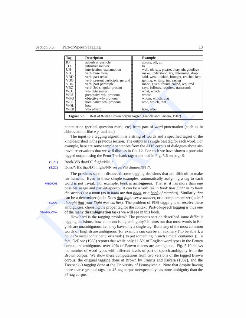
Tag Description ExampleRP adverb or particle across, off, upTO infinitive marker toUH interjection, exclamation well, oh, say, please, okay, uh, goodbyeVB verb, base form make, understand, try, determine, dropVBD verb, past tense said, went, looked, brought, reached keptVBG verb, present participle, gerund getting, writing, increasingVBN verb, past participle made, given, found, called, requiredVBZ verb, 3rd singular present says, follows, requires, transcendsWDT wh- determiner what, whichWP$ possessive wh- pronoun whoseWPO objective wh- pronoun whom, which, thatWPS nominative wh- pronoun who, which, thatWQL howWRB wh- adverb how, when

Figure 5.8 Rest of 87-tag Brown corpus tagset (Francis and Kucera, 1982).

punctuation (period, question mark, etc) from part-of-word punctuation (such as inabbreviations likee.g.andetc.)

The input to a tagging algorithm is a string of words and a specified tagset of thekind described in the previous section. The output is a single best tag for each word. Forexample, here are some sample sentences from the ATIS corpusof dialogues about air-travel reservations that we will discuss in Ch. 12. For each we have shown a potentialtagged output using the Penn Treebank tagset defined in Fig. 5.6 on page 9:

(5.21) Book/VB that/DT flight/NN ./.(5.22) Does/VBZ that/DT flight/NN serve/VB dinner/NN ?/.

The previous section discussed some tagging decisions thatare difficult to makefor humans. Even in these simple examples, automatically assigning a tag to eachword is not trivial. For example,book is ambiguous. That is, it has more than oneAMBIGUOUS

possible usage and part-of-speech. It can be a verb (as inbookthat flightor to bookthe suspect) or a noun (as inhand me that book, or a bookof matches). Similarly thatcan be a determiner (as inDoes thatflight serve dinner), or a complementizer (as inIthought thatyour flight was earlier). The problem of POS-tagging is toresolvetheseRESOLVE

ambiguities, choosing the proper tag for the context. Part-of-speech tagging is thus oneof the manydisambiguation tasks we will see in this book.DISAMBIGUATION

How hard is the tagging problem? The previous section described some difficulttagging decisions; how common is tag ambiguity? It turns outthat most words in En-glish are unambiguous; i.e., they have only a single tag. Butmany of the most commonwords of English are ambiguous (for examplecancan be an auxiliary (‘to be able’), anoun (‘a metal container’), or a verb (‘to put something in such a metal container’)). Infact, DeRose (1988) reports that while only 11.5% of Englishword types in the Browncorpus are ambiguous, over 40% of Brown tokens are ambiguous. Fig. 5.10 showsthe number of word types with different levels of part-of-speech ambiguity from theBrown corpus. We show these computations from two versions of the tagged Browncorpus, the original tagging done at Brown by Francis and Kuˇcera (1982), and theTreebank-3 tagging done at the University of Pennsylvania.Note that despite havingmore coarse-grained tags, the 45-tag corpus unexpectedly has more ambiguity than the87-tag corpus.

DRAFT


Tag Description ExampleAJ0 adjective (unmarked) good, oldAJC comparative adjective better, olderAJS superlative adjective best, oldestAT0 article the, a, anAV0 adverb (unmarked) often, well, longer, furthestAVP adverb particle up, off, outAVQ wh-adverb when, how, whyCJC coordinating conjunction and, orCJS subordinating conjunction although, whenCJT the conjunctionthatCRD cardinal numeral (exceptone) 3, twenty-five, 734DPS possessive determiner your, theirDT0 general determiner these, someDTQ wh-determiner whose, whichEX0 existentialthereITJ interjection or other isolate oh, yes, mhmNN0 noun (neutral for number) aircraft, dataNN1 singular noun pencil, gooseNN2 plural noun pencils, geeseNP0 proper noun London, Michael, MarsORD ordinal sixth, 77th, lastPNI indefinite pronoun none, everythingPNP personal pronoun you, them, oursPNQ wh-pronoun who, whoeverPNX reflexive pronoun itself, ourselvesPOS possessive’s or ’PRF the prepositionofPRP preposition (exceptof) for, above, toPUL punctuation – left bracket ( or [PUN punctuation – general mark . ! , : ; - ? ...PUQ punctuation – quotation mark ‘ ’ ”PUR punctuation – right bracket ) or ]TO0 infinitive markertoUNC unclassified items (not English)VBB base forms ofbe(except infinitive) am, areVBD past form ofbe was, wereVBG -ing form of be beingVBI infinitive of beVBN past participle ofbe beenVBZ -s form ofbe is, ’sVDB/D/G/I/N/Z form of do do, does, did, doing, to do, etc.VHB/D/G/I/N/Z form of have have, had, having, to have, etc.VM0 modal auxiliary verb can, could, will, ’llVVB base form of lexical verb (except infin.) take, liveVVD past tense form of lexical verb took, livedVVG -ing form of lexical verb taking, livingVVI infinitive of lexical verb take, liveVVN past participle form of lex. verb taken, livedVVZ -s form of lexical verb takes, livesXX0 the negativenot or n’tZZ0 alphabetical symbol A, B, c, d

Figure 5.9 UCREL’s C5 tagset for the British National Corpus (Garside et al., 1997).

Luckily, it turns out that many of the 40% ambiguous tokens are easy to disam-biguate. This is because the various tags associated with a word are not equally likely.For example,a can be a determiner, or the lettera (perhaps as part of an acronym or an

DRAFT

Section 5.4. Rule-Based Part-of-Speech Tagging 15

Original Treebank87-tag corpus 45-tag corpus

Unambiguous (1 tag) 44,019 38,857Ambiguous (2–7 tags) 5,490 8844Details: 2 tags 4,967 6,731

3 tags 411 16214 tags 91 3575 tags 17 906 tags 2 (well, beat) 327 tags 2 (still, down) 6 (well, set, round, open, fit,

down)8 tags 4 (’s, half, back, a)9 tags 3 (that, more, in)

Figure 5.10 The amount of tag ambiguity for word types in the Brown corpus, fromthe ICAME release of the original (87-tag) tagging and the Treebank-3 (45-tag) tagging.Numbers are not strictly comparable because only the Treebank segments’s. An earlierestimate of some of these numbers is reported in DeRose (1988).

initial). But the determiner sense ofa is much more likely.Most tagging algorithms fall into one of two classes:rule-basedtaggers andstochas-RULEBASED

tic taggers taggers. Rule-based taggers generally involve a large database of hand-STOCHASTICTAGGERS

written disambiguation rules which specify, for example, that an ambiguous word isa noun rather than a verb if it follows a determiner. The next section will describe asample rule-based tagger,EngCG, based on the Constraint Grammar architecture ofKarlsson et al. (1995b).

Stochastic taggers generally resolve tagging ambiguitiesby using a training cor-pus to compute the probability of a given word having a given tag in a given context.Sec. 5.5 describes the Hidden Markov Model orHMM tagger .HMM TAGGER

Finally, Sec. 5.6 will describe an approach to tagging called thetransformation-based taggeror theBrill tagger , after Brill (1995). The Brill tagger shares featuresBRILL TAGGER

of both tagging architectures. Like the rule-based tagger,it is based on rules whichdetermine when an ambiguous word should have a given tag. Like the stochastic tag-gers, it has a machine-learning component: the rules are automatically induced from apreviously tagged training corpus.

5.4 RULE-BASED PART-OF-SPEECHTAGGING

The earliest algorithms for automatically assigning part-of-speech were based on a two-stage architecture (Harris, 1962; Klein and Simmons, 1963;Greene and Rubin, 1971).The first stage used a dictionary to assign each word a list of potential parts-of-speech.The second stage used large lists of hand-written disambiguation rules to winnow downthis list to a single part-of-speech for each word.

Modern rule-based approaches to part-of-speech tagging have a similar architec-ture, although the dictionaries and the rule sets are vastlylarger than in the 1960’s.

DRAFT


One of the most comprehensive rule-based approaches is the Constraint Grammar ap-proach (Karlsson et al., 1995a). In this section we describea tagger based on thisapproach, theEngCG tagger (Voutilainen, 1995, 1999).ENGCG

The EngCG ENGTWOL lexicon is based on the two-level morphology described inCh. 3, and has about 56,000 entries for English word stems (Heikkila, 1995), countinga word with multiple parts-of-speech (e.g., nominal and verbal senses ofhit) as separateentries, and not counting inflected and many derived forms. Each entry is annotatedwith a set of morphological and syntactic features. Fig. 5.11 shows some selectedwords, together with a slightly simplified listing of their features; these features areused in rule writing.

Word POS Additional POS featuressmaller ADJ COMPARATIVEentire ADJ ABSOLUTE ATTRIBUTIVEfast ADV SUPERLATIVEthat DET CENTRAL DEMONSTRATIVE SGall DET PREDETERMINER SG/PL QUANTIFIERdog’s N GENITIVE SGfurniture N NOMINATIVE SG NOINDEFDETERMINERone-third NUM SGshe PRON PERSONAL FEMININE NOMINATIVE SG3show V PRESENT -SG3 VFINshow N NOMINATIVE SGshown PCP2 SVOO SVO SVoccurred PCP2 SVoccurred V PAST VFIN SV

Figure 5.11 Sample lexical entries from the ENGTWOL lexicon described in Vouti-lainen (1995) and Heikkila (1995).

Most of the features in Fig. 5.11 are relatively self-explanatory; SG for singular,-SG3 for other than third-person-singular. ABSOLUTE meansnon-comparative andnon-superlative for an adjective, NOMINATIVE just means non-genitive, and PCP2means past participle. PRE, CENTRAL, and POST are ordering slots for determiners(predeterminers (all) come before determiners (the): all the president’s men). NOIN-DEFDETERMINER means that words likefurniture do not appear with the indefinitedeterminera. SV, SVO, and SVOO specify thesubcategorizationor complementa-SUBCATEGORIZATION

tion pattern for the verb. Subcategorization will be discussed in Ch. 12 and Ch. 16, butCOMPLEMENTATION

briefly SV means the verb appears solely with a subject (nothing occurred); SVO witha subject and an object (I showed the film); SVOO with a subject and two complements:She showed her the ball.

In the first stage of the tagger, each word is run through the two-level lexicon trans-ducer and the entries for all possible parts-of-speech are returned. For example thephrasePavlov had shown that salivation . . .would return the following list (one lineper possible tag, with the correct tag shown in boldface):

DRAFT

Section 5.4. Rule-Based Part-of-Speech Tagging 17

Pavlov PAVLOV N NOM SG PROPERhad HAVE V PAST VFIN SVO

HAVE PCP2 SVOshown SHOW PCP2 SVOO SVO SVthat ADV

PRON DEM SGDET CENTRAL DEM SGCS

salivation N NOM SG. . .

EngCG then applies a large set of constraints (as many as 3,744 constraints inthe EngCG-2 system) to the input sentence to rule out incorrect parts-of-speech. Theboldfaced entries in the table above show the desired result, in which the simple pasttense tag (rather than the past participle tag) is applied tohad, and the complementizer(CS) tag is applied tothat. The constraints are used in a negative way, to eliminatetags that are inconsistent with the context. For example oneconstraint eliminates allreadings ofthat except the ADV (adverbial intensifier) sense (this is the sense in thesentenceit isn’t that odd). Here’s a simplified version of the constraint:

ADVERBIAL -THAT RULE

Given input: “that”if

(+1 A/ADV/QUANT); /* if next word is adj, adverb, or quantifier*/(+2 SENT-LIM); /* and following which is a sentence boundary,*/(NOT -1 SVOC/A);/* and the previous word is not a verb like*/

/* ‘consider’ which allows adjs as object complements*/then eliminate non-ADV tagselseeliminate ADV tag

The first two clauses of this rule check to see that thethat directly precedes asentence-final adjective, adverb, or quantifier. In all other cases the adverb readingis eliminated. The last clause eliminates cases preceded byverbs likeconsideror be-lieve which can take a noun and an adjective; this is to avoid tagging the followinginstance ofthatas an adverb:

I consider that odd.

Another rule is used to express the constraint that the complementizer sense ofthatis most likely to be used if the previous word is a verb which expects a complement(like believe, think, or show), and if that is followed by the beginning of a noun phrase,and a finite verb.

This description oversimplifies the EngCG architecture; the system also includesprobabilistic constraints, and also makes use of other syntactic information we haven’tdiscussed. The interested reader should consult Karlsson et al. (1995b) and Voutilainen(1999).

DRAFT


5.5 HMM PART-OF-SPEECHTAGGING

The use of probabilities in tags is quite old; probabilitiesin tagging were first used byStolz et al. (1965), a complete probabilistic tagger with Viterbi decoding was sketchedby Bahl and Mercer (1976), and various stochastic taggers were built in the 1980s(Marshall, 1983; Garside, 1987; Church, 1988; DeRose, 1988). This section describesa particular stochastic tagging algorithm generally knownas the Hidden Markov Modelor HMM tagger. Hidden Markov Models themselves will be more fully introduced anddefined in Ch. 6. In this section, we prefigure Ch. 6 a bit by giving an initial introductionto the Hidden Markov Model as applied to part-of-speech tagging.

Use of a Hidden Markov Model to do part-of-speech-tagging, as we will define it, isa special case ofBayesian inference, a paradigm that has been known since the work ofBAYESIAN

INFERENCE

Bayes (1763). Bayesian inference or Bayesian classification was applied successfullyto language problems as early as the late 1950s, including the OCR work of Bledsoein 1959, and the seminal work of Mosteller and Wallace (1964)on applying Bayesianinference to determine the authorship of the Federalist papers.

In a classification task, we are given some observation(s) and our job is to determinewhich of a set of classes it belongs to. Part-of-speech tagging is generally treated as asequence classification task. So here the observation is a sequence of words (let’s saya sentence), and it is our job to assign them a sequence of part-of-speech tags.

For example, say we are given a sentence like

(5.23) Secretariat is expected torace tomorrow.

What is the best sequence of tags which corresponds to this sequence of words?The Bayesian interpretation of this task starts by considering all possible sequencesof classes—in this case, all possible sequences of tags. Outof this universe of tagsequences, we want to chose the tag sequence which is most probable given the obser-vation sequence ofn wordswn

1. In other words, we want, out of all sequences ofn tagstn1 the single tag sequence such thatP(tn

1|wn1) is highest. We use the hat notationˆ toˆ

mean “our estimate of the correct tag sequence”.

tn1 = argmax

tn1

P(tn1|w

n1)(5.24)

The function argmaxx f (x) means “thex such thatf (x) is maximized”. Equation(5.24) thus means, out of all tag sequences of lengthn, we want the particular tagsequencetn

1 which maximizes the right-hand side. While (5.24) is guaranteed to giveus the optimal tag sequence, it is not clear how to make the equation operational; thatis, for a given tag sequencetn

1 and word sequencewn1, we don’t know how to directly

computeP(tn1|w

n1).

The intuition of Bayesian classification is to use Bayes’ rule to transform (5.24)into a set of other probabilities which turn out to be easier to compute. Bayes’ rule ispresented in (5.25); it gives us a way to break down any conditional probabilityP(x|y)into three other probabilities:

P(x|y) =P(y|x)P(x)

P(y)(5.25)

DRAFT

Section 5.5. HMM Part-of-Speech Tagging 19

We can then substitute (5.25) into (5.24) to get (5.26):

tn1 = argmax

tn1

P(wn1|t

n1)P(tn

1)

P(wn1)

(5.26)

We can conveniently simplify 5.26 by dropping the denominator P(wn1). Why is

that? Since we are choosing a tag sequence out of all tag sequences, we will be comput-

ingP(wn

1|tn1)P(tn1)

P(wn1)

for each tag sequence. ButP(wn1) doesn’t change for each tag sequence;

we are always asking about the most likely tag sequence for the same observationwn1,

which must have the same probabilityP(wn1). Thus we can choose the tag sequence

which maximizes this simpler formula:

tn1 = argmax

tn1

P(wn1|t

n1)P(tn

1)(5.27)

To summarize, the most probable tag sequencetn1 given some word stringwn

1 canbe computed by taking the product of two probabilities for each tag sequence, andchoosing the tag sequence for which this product is greatest. The two terms are theprior probability of the tag sequenceP(tn

1)), and thelikelihood of the word stringPRIOR PROBABILITY

LIKELIHOOD P(wn1|t

n1):

tn1 = argmax

tn1

likelihood︷︸︸︷

P(wn1|t

n1)

prior︷︸︸︷

P(tn1)(5.28)

Unfortunately, (5.28) is still too hard to compute directly. HMM taggers thereforemake two simplifying assumptions. The first assumption is that the probability of aword appearing is dependent only on its own part-of-speech tag; that it is independentof other words around it, and of the other tags around it:

P(wn1|t

n1) ≈

n

∏i=1

P(wi |ti)(5.29)

The second assumption is that the probability of a tag appearing is dependent onlyon the previous tag, thebigram assumption we saw in Ch. 4:

P(tn1) ≈

n

∏i=1

P(ti |ti−1)(5.30)

Plugging the simplifying assumptions (5.29) and (5.30) into (5.28) results in thefollowing equation by which a bigram tagger estimates the most probable tag sequence:

tn1 = argmax

tn1

P(tn1|w

n1)≈ argmax

tn1

n

∏i=1

P(wi |ti)P(ti |ti−1)(5.31)

Equation (5.31) contains two kinds of probabilities, tag transition probabilities andword likelihoods. Let’s take a moment to see what these probabilities represent. The

DRAFT


tag transition probabilities,P(ti |ti−1), represent the probability of a tag given the previ-ous tag. For example, determiners are very likely to precedeadjectives and nouns, as insequences likethat/DT flight/NNandthe/DT yellow/JJ hat/NN. Thus we would expectthe probabilitiesP(NN|DT) andP(JJ|DT) to be high. But in English, adjectives don’ttend to precede determiners, so the probabilityP(DT|JJ) ought to be low.

We can compute the maximum likelihood estimate of a tag transition probabilityP(NN|DT) by taking a corpus in which parts-of-speech are labeled and counting, outof the times we see DT, how many of those times we see NN after the DT. That is, wecompute the following ratio of counts:

P(ti |ti−1) =C(ti−1,ti)C(ti−1)

(5.32)

Let’s choose a specific corpus to examine. For the examples inthis chapter we’lluse the Brown corpus, the 1 million word corpus of American English described earlier.The Brown corpus has been tagged twice, once in the 1960’s with the 87-tag tagset, andagain in the 1990’s with the 45-tag Treebank tagset. This makes it useful for comparingtagsets, and is also widely available.

In the 45-tag Treebank Brown corpus, the tag DT occurs 116,454 times. Of these,DT is followed by NN 56,509 times (if we ignore the few cases ofambiguous tags).Thus the MLE estimate of the transition probability is calculated as follows:

P(NN|DT) =C(DT,NN)

C(DT)=

56,509116,454

= .49(5.33)

The probability of getting a common noun after a determiner,.49, is indeed quitehigh, as we suspected.

The word likelihood probabilities,P(wi |ti), represent the probability, given that wesee a given tag, that it will be associated with a given word. For example if we were tosee the tag VBZ (third person singular present verb) and guess the verb that is likely tohave that tag, we might likely guess the verbis, since the verbto beis so common inEnglish.

We can compute the MLE estimate of a word likelihood probability like P(is|VBZ)again by counting, out of the times we see VBZ in a corpus, how many of those timesthe VBZ is labeling the wordis. That is, we compute the following ratio of counts:

P(wi |ti) =C(ti ,wi)

C(ti)(5.34)

In Treebank Brown corpus, the tag VBZ occurs 21,627 times, and VBZ is the tagfor is 10,073 times. Thus:

P(is|VBZ) =C(VBZ, is)C(VBZ)

=10,07321,627

= .47(5.35)

For those readers who are new to Bayesian modeling note that this likelihood termis not asking “which is the most likely tag for the wordis”. That is, the term is notP(VBZ|is). Instead we are computingP(is|VBZ). The probability, slightly counterin-tuitively, answers the question “If we were expecting a third person singular verb, howlikely is it that this verb would beis?”.

DRAFT


We have now defined HMM tagging as a task of choosing a tag-sequence with themaximum probability, derived the equations by which we willcompute this probability,and shown how to compute the component probabilities. In fact we have simplified thepresentation of the probabilities in many ways; in later sections we will return to theseequations and introduce the deleted interpolation algorithm for smoothing these counts,the trigram model of tag history, and a model for unknown words.

But before turning to these augmentations, we need to introduce the decoding algo-rithm by which these probabilities are combined to choose the most likely tag sequence.

5.5.1 Computing the most-likely tag sequence: A motivatingex-ample

The previous section showed that the HMM tagging algorithm chooses as the mostlikely tag sequence the one that maximizes the product of twoterms; the probability ofthe sequence of tags, and the probability of each tag generating a word. In this sectionwe ground these equations in a specific example, showing for aparticular sentence howthe correct tag sequence achieves a higher probability thanone of the many possiblewrong sequences.

We will focus on resolving the part-of-speech ambiguity of the wordrace, whichcan be a noun or verb in English, as we show in two examples modified from the Brownand Switchboard corpus. For this example, we will use the 87-tag Brown corpus tagset,because it has a specific tag forto, TO, used only whento is an infinitive; prepositionaluses ofto are tagged as IN. This will come in handy in our example.1

In (5.36)race is a verb (VB) while in (5.37)race is a common noun (NN):

(5.36) Secretariat/NNP is/BEZ expected/VBN to/TOrace/VB tomorrow/NR

(5.37) People/NNS continue/VB to/TO inquire/VB the/AT reason/NNfor/IN the/ATrace/NN for/IN outer/JJ space/NN

Let’s look at howracecan be correctly tagged as a VB instead of an NN in (5.36).HMM part-of-speech taggers resolve this ambiguity globally rather than locally, pick-ing the best tag sequence for the whole sentence. There are many hypothetically pos-sible tag sequences for (5.36), since there are other ambiguities in the sentence (forexampleexpectedcan be an adjective (JJ), a past tense/preterite (VBD) or a past partici-ple (VBN)). But let’s just consider two of the potential sequences, shown in Fig. 5.12.Note that these sequences differ only in one place; whether the tag chosen forrace isVB or NN.

Almost all the probabilities in these two sequences are identical; in Fig. 5.12 wehave highlighted in boldface the three probabilities that differ. Let’s consider twoof these, corresponding toP(ti |ti−1) and P(wi |ti). The probabilityP(ti |ti−1) in Fig-ure 5.12a isP(VB|TO), while in Figure 5.12b the transition probability isP(NN|TO).

The tag transition probabilitiesP(NN|TO) andP(VB|TO) give us the answer to thequestion “How likely are we to expect a verb (noun) given the previous tag?” As we

1 The 45-tag Treebank-3 tagset does make this distinction in the Switchboard corpus but not, alas, in theBrown corpus. Recall that in the 45-tag tagset time adverbs like tomorroware tagged as NN; in the 87-tagtagset they appear as NR.

DRAFT


Figure 5.12 Two of the possible sequences of tags corresponding to the Secretariatsentence, one of them corresponding to the correct sequence, in which race is a VB. Eacharc in these graphs would be associated with a probability. Note that the two graphs differonly in 3 arcs, hence in 3 probabilities.

saw in the previous section, the maximum likelihood estimate for these probabilitiescan be derived from corpus counts.

Since the (87-tag Brown tagset) tag TO is used only for the infinitive markerto, weexpect that only a very small number of nouns can follow this marker (as an exercise,try to think of a sentence where a noun can follow the infinitive marker use ofto).Sure enough, a look at the (87-tag) Brown corpus gives us the following probabilities,showing that verbs are about 500 times as likely as nouns to occur after TO:

P(NN|TO) = .00047

P(VB|TO) = .83

Let’s now turn toP(wi |ti), the lexical likelihood of the wordracegiven a part-of-speech tag. For the two possible tags VB and NN, these correspond to the probabilitiesP(race|VB) andP(race|NN). Here are the lexical likelihoods from Brown:

P(race|NN) = .00057

P(race|VB) = .00012

Finally, we need to represent the tag sequence probability for the following tag (in thiscase the tag NR fortomorrow):

P(NR|VB) = .0027

P(NR|NN) = .0012

DRAFT


If we multiply the lexical likelihoods with the tag sequenceprobabilities, we seethat the probability of the sequence with the VB tag is higherand the HMM taggercorrectly tagsraceas a VB in Fig. 5.12 despite the fact that it is the less likely sense ofrace:

P(VB|TO)P(NR|VB)P(race|VB) = .00000027

P(NN|TO)P(NR|NN)P(race|NN) = .00000000032

5.5.2 Formalizing Hidden Markov Model taggers

Now that we have seen the equations and some examples of choosing the most probabletag sequence, we show a brief formalization of this problem as a Hidden Markov Model(see Ch. 6 for the more complete formalization).

The HMM is an extension of the finite automata of Ch. 3. Recall that a finiteautomaton is defined by a set of states, and a set of transitions between states that aretaken based on the input observations. Aweighted finite-state automatonis a simpleWEIGHTED

augmentation of the finite automaton in which each arc is associated with a probability,indicating how likely that path is to be taken. The probability on all the arcs leavinga node must sum to 1. AMarkov chain is a special case of a weighted automatonMARKOV CHAIN

in which the input sequence uniquely determines which states the automaton will gothrough. Because they can’t represent inherently ambiguous problems, a Markov chainis only useful for assigning probabilities to unambiguous sequences.

While the Markov chain is appropriate for situations where we can see the actualconditioning events, it is not appropriate in part-of-speech tagging. This is because inpart-of-speech tagging, while we observe the words in the input, we donot observethe part-of-speech tags. Thus we can’t condition any probabilities on, say, a previouspart-of-speech tag, because we cannot be completely certain exactly which tag appliedto the previous word. AHidden Markov Model (HMM ) allows us to talk about bothHIDDEN MARKOV

MODEL

observedevents (like words that we see in the input) andhiddenevents (like part-of-speech tags) that we think of as causal factors in our probabilistic model.

An HMM is specified by the following components:HMM

DRAFT


Q = q1q2 . . .qN a set ofN states

A = a11a12. . .an1 . . .ann a transition probability matrix A, eachai j rep-resenting the probability of moving from stateito statej, s.t.∑n

j=1ai j = 1 ∀i

O = o1o2 . . .oT a sequence ofT observations, each one drawnfrom a vocabularyV = v1,v2, ...,vV .

B = bi(ot) A sequence ofobservation likelihoods:, alsocalled emission probabilities, each expressingthe probability of an observationot being gen-erated from a statei.

q0,qF a specialstart state andend (final) statewhichare not associated with observations, togetherwith transition probabilitiesa01a02..a0n out of thestart state anda1Fa2F ...anF into the end state.

Figure 5.13 The weighted finite-state network corresponding to the hidden states of theHMM. The A transition probabilities are used to compute the prior probability.

An HMM thus has two kinds of probabilities; theA transition probabilities, andtheB observation likelihoods, corresponding respectively to theprior andlikelihoodprobabilities that we saw in equation (5.31). Fig. 5.13 illustrates the prior probabilitiesin an HMM part-of-speech tagger, showing 3 sample states andsome of theA transitionprobabilities between them. Fig. 5.14 shows another view ofan HMM part-of-speechtagger, focusing on the word likelihoodsB. Each hidden state is associated with avector of likelihoods for each observation word.

5.5.3 The Viterbi Algorithm for HMM Tagging

For any model, such as an HMM, that contains hidden variables, the task of determin-ing which sequence of variables is the underlying source of some sequence of observa-tions is called thedecodingtask. TheViterbi algorithm is perhaps the most commonDECODING

VITERBI decoding algorithm used for HMMs, whether for part-of-speech tagging or for speechrecognition. The termViterbi is common in speech and language processing, but this

DRAFT


Figure 5.14 TheB observation likelihoods for the HMM in the previous figure. Eachstate (except the non-emitting Start and End states) is associated with a vector of probabil-ities, one likelihood for each possible observation word.

is really a standard application of the classicdynamic programming algorithm, andlooks a lot like theminimum edit distance algorithm of Ch. 3. The Viterbi algorithmwas first applied to speech and language processing in the context of speech recogni-tion by Vintsyuk (1968), but has what Kruskal (1983) calls a ‘remarkable history ofmultiple independent discovery and publication’; see the History section at the end ofCh. 6 for more details.

The slightly simplified version of the Viterbi algorithm that we will present takesas input a single HMM and a set of observed wordsO= (o1o2o3 . . .oT) and returns themost probable state/tag sequenceQ = (q1q2q3 . . .qT), together with its probability.

Let the HMM be defined by the two tables in Fig. 5.15 and Fig. 5.16. Fig. 5.15expresses theai j probabilities, thetransition probabilities between hidden states (i.e.part-of-speech tags). Fig. 5.16 expresses thebi(ot) probabilities, theobservationlike-lihoods of words given tags.

VB TO NN PPSS<s> .019 .0043 .041 .067VB .0038 .035 .047 .0070TO .83 0 .00047 0NN .0040 .016 .087 .0045PPSS .23 .00079 .0012 .00014

Figure 5.15 Tag transition probabilities (thea array,p(ti |ti−1)) computed from the 87-tag Brown corpus without smoothing. The rows are labeled with the conditioning event;thusP(PPSS|VB) is .0070. The symbol<s> is the start-of-sentence symbol.

Fig. 5.17 shows pseudocode for the Viterbi algorithm. The Viterbi algorithm sets

DRAFT


I want to raceVB 0 .0093 0 .00012TO 0 0 .99 0NN 0 .000054 0 .00057PPSS .37 0 0 0

Figure 5.16 Observation likelihoods (theb array) computed from the 87-tag Browncorpus without smoothing.

function V ITERBI(observationsof lenT,state-graphof lenN) returns best-path

create a path probability matrixviterbi[N+2,T]for each states from 1 to N do ;initialization step

viterbi[s,1]←a0,s ∗ bs(o1)backpointer[s,1]←0

for each time stept from 2 to T do ;recursion stepfor each states from 1 to N do

viterbi[s,t]←N

maxs′=1

viterbi[s′,t−1] ∗ as′,s ∗ bs(ot )

backpointer[s,t]←N

argmaxs′=1

viterbi[s′,t−1] ∗ as′,s

viterbi[qF ,T]←N

maxs=1

viterbi[s,T] ∗ as,qF ; termination step

backpointer[qF ,T]←N

argmaxs=1

viterbi[s,T] ∗ as,qF ; termination step

return the backtrace path by following backpointers to states backin time frombackpointer[qF ,T]

Figure 5.17 Viterbi algorithm for finding optimal sequence of tags. Given an observa-tion sequence and an HMMλ = (A,B), the algorithm returns the state-path through theHMM which assigns maximum likelihood to the observation sequence. Note that states 0andqF are non-emitting.

up a probability matrix, with one column for each observation t and one row for eachstate in the state graph. Each column thus has a cell for each state qi in the singlecombined automaton for the four words.

The algorithm first createsN or four state columns. The first column correspondsto the observation of the first wordi, the second to the second wordwant, the third tothe third wordto, and the fourth to the fourth wordrace. We begin in the first columnby setting the viterbi value in each cell to the product of thetransition probability (intoit from the state state) and the observation probability (ofthe first word); the readershould find this in Fig. 5.18.

Then we move on, column by column; for every state in column 1,we compute theprobability of moving into each state in column 2, and so on. For each stateq j at timet, the valueviterbi[s, t] is computed by taking the maximum over the extensions of allthe paths that lead to the current cell, following the following equation:

DRAFT


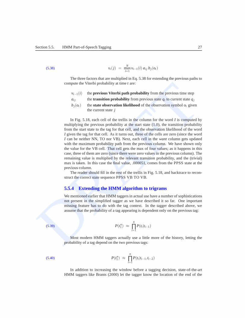
vt( j) =N

maxi=1

vt−1(i) ai j b j(ot)(5.38)

The three factors that are multiplied in Eq. 5.38 for extending the previous paths tocompute the Viterbi probability at timet are:

vt−1(i) theprevious Viterbi path probability from the previous time step

ai j thetransition probability from previous stateqi to current stateq j

b j(ot) thestate observation likelihoodof the observation symbolot giventhe current statej

In Fig. 5.18, each cell of the trellis in the column for the word I is computed bymultiplying the previous probability at the start state (1.0), the transition probabilityfrom the start state to the tag for that cell, and the observation likelihood of the wordI given the tag for that cell. As it turns out, three of the cellsare zero (since the wordI can be neither NN, TO nor VB). Next, each cell in thewant column gets updatedwith the maximum probability path from the previous column.We have shown onlythe value for the VB cell. That cell gets the max of four values; as it happens in thiscase, three of them are zero (since there were zero values in the previous column). Theremaining value is multiplied by the relevant transition probability, and the (trivial)max is taken. In this case the final value, .000051, comes fromthe PPSS state at theprevious column.

The reader should fill in the rest of the trellis in Fig. 5.18, and backtrace to recon-struct the correct state sequence PPSS VB TO VB.

5.5.4 Extending the HMM algorithm to trigrams

We mentioned earlier that HMM taggers in actual use have a number of sophisticationsnot present in the simplified tagger as we have described it sofar. One importantmissing feature has to do with the tag context. In the tagger described above, weassume that the probability of a tag appearing is dependent only on the previous tag:

P(tn1) ≈

n

∏i=1

P(ti |ti−1)(5.39)

Most modern HMM taggers actually use a little more of the history, letting theprobability of a tag depend on the two previous tags:

P(tn1) ≈

n

∏i=1

P(ti |ti−1,ti−2)(5.40)

In addition to increasing the window before a tagging decision, state-of-the-artHMM taggers like Brants (2000) let the tagger know the location of the end of the

DRAFT


start

VB

PP

SS

VB

PP

SS

VB

PP

SS

end

P(PPSS|start) * P(start)

.067 x 1.0 = .067

v1(2) x P(VB|VB)

0 x .0038 = 0

v1(1) x P(V

B|PPSS)

.025 x .23 = .0055

P(VB|start)xP(start)

.019 x 1.0 = .019

v1(2)=.019 x 0 = 0

v1(1) = .067 x .37 = .025

v2(2)= max(0,0,0,.0055) x .0093 = .000051

start start start

t

PPS

S

VB

end end endqend

q2

q1

q0

o1

i racewant

o2 o3

VB

PP

SS

start

end

to

TO TO TOTO TO

NN NN NNNN NN

v1(3)=.0043 x 0 = 0

v1(4)=.041 x 0=0

o4

v1(3) * P(VB|TO)

0 x .83 = 0

v1(4) * P(VB|NN)

0 x .0040 = 0

v0(0) = 1.0

P(TO|start)xP(start)

.0043 x 1.0 = .0043

P(NN|start)xP(start)

.041 x 1.0 = .041

backtrace

backtrace

q3

q4

Figure 5.18 The entries in the individual state columns for the Viterbi algorithm. Each cell keeps the probabil-ity of the best path so far and a pointer to the previous cell along that path. We have only filled out columns 0 and1 and one cell of column 2; the rest is left as an exercise for the reader. After the cells are filled in, backtracingfrom theendstate, we should be able to reconstruct the correct state sequence PPSS VB TO VB.

sentence by adding dependence on an end-of-sequence markerfor tn+1. This gives thefollowing equation for part of speech tagging:

tn1 = argmax

tn1

P(tn1|w

n1)≈ argmax

tn1

[n

∏i=1

P(wi |ti)P(ti |ti−1,ti−2)

]

P(tn+1|tn)(5.41)

In tagging any sentence with (5.41), three of the tags used inthe context will fall offthe edge of the sentence, and hence will not match regular words. These tags,t−1, t0,andtn+1, can all be set to be a single special ‘sentence boundary’ tagwhich is added tothe tagset. This requires that sentences passed to the tagger have sentence boundaries

DRAFT


demarcated, as discussed in Ch. 3.There is one large problem with (5.41); data sparsity. Any particular sequence of

tagsti−2, ti−1, ti that occurs in the test set may simply never have occurred in the trainingset. That means we cannot compute the tag trigram probability just by the maximumlikelihood estimate from counts, following Equation (5.42):

P(ti |ti−1,ti−2) =C(ti−2,ti−1,ti)C(ti−2,ti−1)

:(5.42)

Why not? Because many of these counts will be zero in any training set, and we willincorrectly predict that a given tag sequence will never occur! What we need is a wayto estimateP(ti |ti−1, ti−2) even if the sequenceti−2,ti−1,ti never occurs in the trainingdata.

The standard approach to solve this problem is to estimate the probability by com-bining more robust, but weaker estimators. For example, if we’ve never seen the tagsequence PRP VB TO, so we can’t computeP(TO|PRP,VB) from this frequency, westill could rely on the bigram probabilityP(TO|VB), or even the unigram probabil-ity P(TO). The maximum likelihood estimation of each of these probabilities can becomputed from a corpus via the following counts:

Trigrams P(ti |ti−1,ti−2) =C(ti−2,ti−1,ti)C(ti−2,ti−1)

(5.43)

Bigrams P(ti |ti−1) =C(ti−1,ti)C(ti−1)

(5.44)

Unigrams P(ti) =C(ti)

N(5.45)

How should these three estimators be combined in order to estimate the trigramprobabilityP(ti |ti−1, ti−2)? The simplest method of combination is linear interpolation.In linear interpolation, we estimate the probabilityP(ti |ti−1ti−2) by a weighted sum ofthe unigram, bigram, and trigram probabilities:

P(ti |ti−1ti−2) = λ1P(ti |ti−1ti−2)+ λ2P(ti |ti−1)+ λ3P(ti)(5.46)

We requireλ1 + λ2+ λ3 = 1, insuring that the resulting P is a probability distribu-tion. How should theseλs be set? One good way isdeleted interpolation, developedDELETED

INTERPOLATION

by Jelinek and Mercer (1980). In deleted interpolation, we successively delete eachtrigram from the training corpus, and choose theλs so as to maximize the likelihoodof the rest of the corpus. The idea of the deletion is to set theλs in such a way as togeneralize to unseen data and not overfit the training corpus. Fig. 5.19 gives the Brants(2000) version of the deleted interpolation algorithm for tag trigrams.

Brants (2000) achieves an accuracy of 96.7% on the Penn Treebank with a trigramHMM tagger. Weischedel et al. (1993) and DeRose (1988) have also reported accu-racies of above 96% for HMM tagging. (Thede and Harper, 1999)offer a number ofaugmentations of the trigram HMM model, including the idea of conditioning wordlikelihoods on neighboring words and tags.

DRAFT


function DELETED-INTERPOLATION(corpus) returns λ1,λ2,λ3

λ1←0λ2←0λ3←0foreach trigramt1,t2,t3 with f (t1,t2,t3) > 0

dependingon the maximum of the following three values

caseC(t1,t2,t3)−1C(t1,t2)−1 : incrementλ3 by C(t1,t2,t3)

caseC(t2,t3)−1C(t2)−1 : incrementλ2 by C(t1,t2,t3)

caseC(t3)−1N−1 : incrementλ1 by C(t1,t2,t3)

endendnormalizeλ1,λ2,λ3return λ1,λ2,λ3

Figure 5.19 The deleted interpolation algorithm for setting the weights for combiningunigram, bigram, and trigram tag probabilities. If the denominator is 0 for any case, wedefine the result of that case to be 0. N is the total number of tokens in the corpus. AfterBrants (2000).

The HMM taggers we have seen so far are trained on hand-taggeddata. Kupiec(1992), Cutting et al. (1992), and others show that it is alsopossible to train an HMMtagger on unlabeled data, using the EM algorithm that we willintroduce in Ch. 6. Thesetaggers still start with a dictionary which lists which tagscan be assigned to whichwords; the EM algorithm then learns the word likelihood function for each tag, andthe tag transition probabilities. An experiment by Merialdo (1994), however, indicatesthat with even a small amount of training data, a tagger trained on hand-tagged dataworked better than one trained via EM. Thus the EM-trained “pure HMM” tagger isprobably best suited to cases where no training data is available, for example whentagging languages for which there is no previously hand-tagged data.

5.6 TRANSFORMATION-BASED TAGGING

Transformation-Based Tagging, sometimes called Brill tagging, is an instance of theTransformation-Based Learning (TBL) approach to machine learning (Brill, 1995),TRANSFORMATION

BASED LEARNING

and draws inspiration from both the rule-based and stochastic taggers. Like the rule-based taggers, TBL is based on rules that specify what tags should be assigned towhat words. But like the stochastic taggers, TBL is a machinelearning technique,in which rules are automatically induced from the data. Likesome but not all of theHMM taggers, TBL is a supervised learning technique; it assumes a pre-tagged trainingcorpus.

Samuel et al. (1998) offer a useful analogy for understanding the TBL paradigm,which they credit to Terry Harvey. Imagine an artist painting a picture of a white house

DRAFT

Section 5.6. Transformation-Based Tagging 31

with green trim against a blue sky. Suppose most of the picture was sky, and hencemost of the picture was blue. The artist might begin by using avery broad brush andpainting the entire canvas blue. Next she might switch to a somewhat smaller whitebrush, and paint the entire house white. She would just colorin the whole house, notworrying about the brown roof, or the blue windows or the green gables. Next shetakes a smaller brown brush and colors over the roof. Now she takes up the blue painton a small brush and paints in the blue windows on the house. Finally she takes a veryfine green brush and does the trim on the gables.

The painter starts with a broad brush that covers a lot of the canvas but colors alot of areas that will have to be repainted. The next layer colors less of the canvas,but also makes less “mistakes”. Each new layer uses a finer brush that corrects less ofthe picture, but makes fewer mistakes. TBL uses somewhat thesame method as thispainter. The TBL algorithm has a set of tagging rules. A corpus is first tagged usingthe broadest rule, that is, the one that applies to the most cases. Then a slightly morespecific rule is chosen, which changes some of the original tags. Next an even narrowerrule, which changes a smaller number of tags (some of which might be previouslychanged tags).

5.6.1 How TBL Rules Are Applied

Let’s look at one of the rules used by Brill’s (1995) tagger. Before the rules apply, thetagger labels every word with its most-likely tag. We get these most-likely tags from atagged corpus. For example, in the Brown corpus,race is most likely to be a noun:

P(NN|race) = .98

P(VB|race) = .02

This means that the two examples ofracethat we saw above will both be coded asNN. In the first case, this is a mistake, as NN is the incorrect tag:

(5.47) is/VBZ expected/VBN to/TO race/NN tomorrow/NN

In the second case thisrace is correctly tagged as an NN:

(5.48) the/DT race/NN for/IN outer/JJ space/NN

After selecting the most-likely tag, Brill’s tagger applies its transformation rules.As it happens, Brill’s tagger learned a rule that applies exactly to this mistagging ofrace:

ChangeNN to VB when the previous tag isTO

This rule would changerace/NNto race/VBin exactly the following situation, sinceit is preceded byto/TO:

(5.49) expected/VBN to/TO race/NN→ expected/VBN to/TO race/VB

5.6.2 How TBL Rules Are Learned

Brill’s TBL algorithm has three major stages. It first labelsevery word with its most-likely tag. It then examines every possible transformation, and selects the one that

DRAFT


results in the most improved tagging. Finally, it then re-tags the data according to thisrule. The last two stages are repeated until some stopping criterion is reached, such asinsufficient improvement over the previous pass. Note that stage two requires that TBLknows the correct tag of each word; that is, TBL is a supervised learning algorithm.

The output of the TBL process is an ordered list of transformations; these thenconstitute a “tagging procedure” that can be applied to a newcorpus. In principle theset of possible transformations is infinite, since we could imagine transformations suchas “transform NN to VB if the previous word was “IBM” and the word “the” occursbetween 17 and 158 words before that”. But TBL needs to consider every possibletransformation, in order to pick the best one on each pass through the algorithm. Thusthe algorithm needs a way to limit the set of transformations. This is done by designinga small set oftemplates(abstracted transformations). Every allowable transformationTEMPLATES

is an instantiation of one of the templates. Brill’s set of templates is listed in Fig. 5.20.Fig. 5.21 gives the details of this algorithm for learning transformations.

The preceding (following) word is taggedz.The word two before (after) is taggedz.One of the two preceding (following) words is taggedz.One of the three preceding (following) words is taggedz.The preceding word is taggedz and the following word is taggedw.The preceding (following) word is taggedz and the word

two before (after) is taggedw.

Figure 5.20 Brill’s (1995) templates. Each begins with“Change taga to tagb when:. . . ” . The variablesa, b, z, andw range over parts-of-speech.

At the heart of Fig. 5.21 are the two functions GET BEST TRANSFORMATION

and GET BEST INSTANCE. GET BEST TRANSFORMATION is called with a list ofpotential templates; for each template, it calls GET BEST INSTANCE. GET BEST -INSTANCE iteratively tests every possible instantiation of each template by filling inspecific values for the tag variablesa, b, z, andw.

In practice, there are a number of ways to make the algorithm more efficient. Forexample, templates and instantiated transformations can be suggested in a data-drivenmanner; a transformation-instance might only be suggestedif it would improve the tag-ging of some specific word. The search can also be made more efficient by pre-indexingthe words in the training corpus by potential transformation. Roche and Schabes (1997)show how the tagger can also be speeded up by converting each rule into a finite-statetransducer and composing all the transducers.

Fig. 5.22 shows a few of the rules learned by Brill’s originaltagger.

5.7 EVALUATION AND ERROR ANALYSIS

The probabilities in a statistical model like an HMM POS-tagger come from the corpusit is trained on. We saw in Sec.?? that in order to train statistical models like taggersor N-grams, we need to set aside atraining set. The design of the training set or

DRAFT

Section 5.7. Evaluation and Error Analysis 33

function TBL(corpus) returns transforms-queueINTIALIZE -WITH-MOST-LIKELY -TAGS(corpus)until end condition is metdotemplates←GENERATE-POTENTIAL-RELEVANT-TEMPLATES

best-transform←GET-BEST-TRANSFORM(corpus, templates)APPLY-TRANSFORM(best-transform,corpus)ENQUEUE(best-transform-rule, transforms-queue)

endreturn (transforms-queue)

function GET-BEST-TRANSFORM(corpus, templates) returns transformfor each templatein templates

(instance,score)←GET-BEST-INSTANCE(corpus, template)if (score> best-transform.score) then best-transform← (instance,score)

return (best-transform)

function GET-BEST-INSTANCE(corpus, template)returns transformfor from-tag← from tag1 to tagn dofor to-tag← from tag1 to tagn do

for pos← from 1 to corpus-sizedoif (correct-tag(pos) == to-tag&& current-tag(pos) == from-tag)

num-good-transforms(current-tag(pos−1))++elseif(correct-tag(pos)==from-tag&& current-tag(pos)==from-tag)

num-bad-transforms(current-tag(pos−1))++endbest-Z←ARGMAX t(num-good-transforms(t) - num-bad-transforms(t))if (num-good-transforms(best-Z) - num-bad-transforms(best-Z)

> best-instance.score) thenbest.rule← “Change tag fromfrom-tagto to-tag if prev tag is best-Z”best.score←num-good-transforms(best-Z) - num-bad-transforms(best-Z)

return (best)

procedure APPLY-TRANSFORM(transform,corpus)for pos← from 1 to corpus-sizedoif (current-tag(pos)==best-rule-from)

&& ( current-tag(pos−1)==best-rule-prev))current-tag(pos)←best-rule-to

Figure 5.21 The TBL algorithm for learning to tag. GET BEST INSTANCEwould haveto change for transformation templates other than“Change tag from X to Y if previous tagis Z” . After Brill (1995).

training corpus needs to be carefully considered. If the training corpus is too specificto the task or domain, the probabilities may be too narrow andnot generalize well totagging sentences in very different domains. But if the training corpus is too general,

DRAFT


Change tags# From To Condition Example1 NN VB Previous tag is TO to/TO race/NN→ VB2 VBP VB One of the previous 3 tags is MD might/MD vanish/VBP→ VB3 NN VB One of the previous 2 tags is MD might/MD not reply/NN→ VB4 VB NN One of the previous 2 tags is DT5 VBD VBN One of the previous 3 tags is VBZ

Figure 5.22 The first 20 nonlexicalized transformations from Brill (1995).

the probabilities may not do a sufficient job of reflecting thetask or domain.For evaluatingN-grams models, we said in Sec.?? that we need to divide our

corpus into a distinct training set, test set, and a second test set called a developmenttest set. We train our tagger on the training set. Then we use the development testset (also called adevtestset) to perhaps tune some parameters, and in general decideDEVELOPMENT TEST

SET

DEVTEST what the best model is. Then once we come up with what we think is the best model,we run it on the (hitherto unseen) test set to see its performance. We might use 80%of our data for training, and save 10% each for devtest and test. Why do we need adevelopment test set distinct from the final test set? Because if we used the final testset to compute performance for all our experiments during our development phase, wewould be tuning the various changes and parameters to this set. Our final error rate onthe test set would then be optimistic: it would underestimate the true error rate.

The problem with having a fixed training set, devset, and testset is that in order tosave lots of data for training, the test set might not be largeenough to be representative.Thus a better approach would be to somehow useall our data both for training andtest. How is this possible? The idea is to usecrossvalidation. In crossvalidation, weCROSSVALIDATION

randomly choose a training and test set division of our data,train our tagger, and thencompute the error rate on the test set. Then we repeat with a different randomly selectedtraining set and test set. We do this sampling process 10 times, and then average these10 runs to get an average error rate. This is called10-fold crossvalidation.10FOLD

CROSSVALIDATION

The only problem with cross-validation is that because all the data is used for test-ing, we need the whole corpus to be blind; we can’t examine anyof the data to suggestpossible features, and in general see what’s going on. But looking at the corpus is of-ten important for designing the system. For this reason it iscommon to create a fixedtraining set and test set, and then to do 10-fold crossvalidation inside the training set,but compute error rate the normal way in the test set.

Once we have a test set, taggers are evaluated by comparing their labeling of the testset with a human-labeledGold Standard test set, based onaccuracy: the percentageof all tags in the test set where the tagger and the Gold standard agree. Most currenttagging algorithms have an accuracy of around 96–97% for simple tagsets like the PennTreebank set. These accuracies are for words and punctuation; the accuracy for wordsonly would be lower.

How good is 97%? Since tagsets and tasks differ, the performance of tags can becompared against a lower-boundbaselineand an upper-boundceiling. One way to setBASELINE

CEILING a ceiling is to see how well humans do on the task. Marcus et al.(1993), for example,found that human annotators agreed on about 96–97% of the tags in the Penn Treebank

DRAFT

Section 5.7. Evaluation and Error Analysis 35

version of the Brown corpus. This suggests that the Gold Standard may have a 3-4%margin of error, and that it is meaningless to get 100% accuracy, (modeling the last3% would just be modeling noise). Indeed Ratnaparkhi (1996)showed that the taggingambiguities that caused problems for his tagger were exactly the ones that humans hadlabeled inconsistently in the training set. Two experiments by Voutilainen (1995, p.174), however, found that when humans were allowed to discuss tags, they reachedconsensus on 100% of the tags.

Human Ceiling: When using a human Gold Standard to evaluate a classificationalgorithm, check the agreement rate of humans on the standard.

The standardbaseline, suggested by Gale et al. (1992) (in the slightly differentcontext of word-sense disambiguation), is to choose theunigram most-likely tag foreach ambiguous word. The most-likely tag for each word can becomputed from ahand-tagged corpus (which may be the same as the training corpus for the tagger beingevaluated).

Most Frequent Class Baseline:Always compare a classifier against a baselineat least as good as the most frequent class baseline (assigning each token to theclass it occurred in most often in the training set).

Tagging algorithms since Harris (1962) incorporate this tag frequency intuition.Charniak et al. (1993) showed that this baseline algorithm achieves an accuracy of 90–91% on the 87-tag Brown tagset; Toutanova et al. (2003) showed that a more complexversion, augmented with an unknown word model, achieved 93.69% on the 45-tagTreebank tagset.

When comparing models it is important to use statistical tests (introduced in anystatistics class or textbook for the social sciences) to determine if the difference be-tween two models is significant. Cohen (1995) is a useful reference which focuseson statistical research methods for artificial intelligence. Dietterich (1998) focuses onstatistical tests for comparing classifiers.

5.7.1 Error Analysis

In order to improve any model we need to understand where it went wrong. Analyzingthe error in a classifier like a part-of-speech tagger is donevia a confusion matrix,or contingency table. A confusion matrix for anN-way classification task is anN-by-N matrix where the cell(x,y) contains the number of times an item with correctclassificationxwas classified by the model asy. For example, the following table showsa portion of the confusion matrix from the HMM tagging experiments of Franz (1996).The row labels indicate correct tags, column labels indicate the tagger’s hypothesizedtags, and each cell indicates percentage of the overall tagging error. Thus 4.4% ofthe total errors were caused by mistagging a VBD as a VBN. Common errors areboldfaced.

DRAFT


IN JJ NN NNP RB VBD VBNIN - .2 .7JJ .2 - 3.3 2.1 1.7 .2 2.7NN 8.7 - .2NNP .2 3.3 4.1 - .2RB 2.2 2.0 .5 -VBD .3 .5 - 4.4VBN 2.8 2.6 -

The confusion matrix above, and related error analyses in Franz (1996), Kupiec(1992), and Ratnaparkhi (1996), suggest that some major problems facing current tag-gers are:

1. NN versus NNP versus JJ:These are hard to distinguish prenominally. Dis-tinguishing proper nouns is especially important for information extraction andmachine translation.

2. RP versus RB versus IN:All of these can appear in sequences of satellitesimmediately following the verb.

3. VBD versus VBN versus JJ:Distinguishing these is important for partial pars-ing (participles are used to find passives), and for correctly labeling the edges ofnoun-phrases.

Error analysis like this is a crucial part of any computational linguistic application. Er-ror analysis can help find bugs, find problems in the training data, and, most important,help in developing new kinds of knowledge or algorithms to use in solving problems.

5.8 ADVANCED ISSUES INPART-OF-SPEECHTAGGING

5.8.1 Practical Issues: Tag Indeterminacy and Tokenization

Tag indeterminacy arises when a word is ambiguous between multiple tags and it isimpossible or very difficult to disambiguate. In this case, some taggers allow the useof multiple tags. This is the case in both the Penn Treebank and in the British NationalCorpus. Common tag indeterminacies include adjective versus preterite versus pastparticiple (JJ/VBD/VBN), and adjective versus noun as prenominal modifier (JJ/NN).Given a corpus with these indeterminate tags, there are 3 ways to deal with tag indeter-minacy when training and scoring part-of-speech taggers:

1. Somehow replace the indeterminate tags with only one tag.

2. In testing, count a tagger as having correctly tagged an indeterminate token if itgives either of the correct tags. In training, somehow choose only one of the tagsfor the word.

3. Treat the indeterminate tag as a single complex tag.

The second approach is perhaps the most sensible, although most previous publishedresults seem to have used the third approach. This third approach applied to the PennTreebank Brown corpus, for example, results in a much largertagset of 85 tags instead

DRAFT

Section 5.8. Advanced Issues in Part-of-Speech Tagging 37

of 45, but the additional 40 complex tags cover a total of only121 word instances outof the million word corpus.

Most tagging algorithms assume a process of tokenization has been applied to thetags. Ch. 3 discussed the issue of tokenization of periods for distinguishing sentence-final periods from word-internal period in words likeetc.. An additional role for tok-enization is in word splitting. The Penn Treebank and the British National Corpus splitcontractions and the’s-genitive from their stems:

would/MD n’t/RBchildren/NNS ’s/POS

Indeed, the special Treebank tag POS is used only for the morpheme’s which mustbe segmented off during tokenization.

Another tokenization issue concerns multi-part words. TheTreebank tagset as-sumes that tokenization of words likeNew Yorkis done at whitespace. The phrasea New York City firmis tagged in Treebank notation as five separate words:a/DTNew/NNP York/NNP City/NNP firm/NN. The C5 tagset, by contrast, allow prepositionslike “ in terms of” to be treated as a single word by adding numbers to each tag, as inin/II31 terms/II32 of/II33.

5.8.2 Unknown Wordswords peoplenever use —could beonly Iknow them

Ishikawa Takuboku 1885–1912All the tagging algorithms we have discussed require a dictionary that lists the

possible parts-of-speech of every word. But the largest dictionary will still not containevery possible word, as we saw in Ch. 7. Proper names and acronyms are created veryoften, and even new common nouns and verbs enter the languageat a surprising rate.Therefore in order to build a complete tagger we cannot always use a dictionary to giveus p(wi |ti). We need some method for guessing the tag of an unknown word.

The simplest possible unknown-word algorithm is to pretendthat each unknownword is ambiguous among all possible tags, with equal probability. Then the taggermust rely solely on the contextual POS-trigrams to suggest the proper tag. A slightlymore complex algorithm is based on the idea that the probability distribution of tagsover unknown words is very similar to the distribution of tags over words that oc-curred only once in a training set, an idea that was suggestedby both Baayen andSproat (1996) and Dermatas and Kokkinakis (1995). These words that only occur onceare known ashapax legomena(singularhapax legomenon). For example, unknownHAPAX LEGOMENA

words andhapax legomenaare similar in that they are both most likely to be nouns,followed by verbs, but are very unlikely to be determiners orinterjections. Thus thelikelihood P(wi |ti) for an unknown word is determined by the average of the distribu-tion over all singleton words in the training set. This idea of using “things we’ve seenonce” as an estimator for “things we’ve never seen” will prove useful in the Good-Turing algorithm of Ch. 4.

DRAFT


Most unknown-word algorithms, however, make use of a much more powerfulsource of information: the morphology of the words. For example, words that endin -s are likely to be plural nouns (NNS), words ending with-ed tend to be past par-ticiples (VBN), words ending withable tend to be adjectives (JJ), and so on. Even ifwe’ve never seen a word, we can use facts about its morphological form to guess itspart-of-speech. Besides morphological knowledge, orthographic information can bevery helpful. For example words starting with capital letters are likely to be propernouns (NP). The presence of a hyphen is also a useful feature;hyphenated words in theTreebank version of Brown are most likely to be adjectives (JJ). This prevalence of JJsis caused by the labeling instructions for the Treebank, which specified that prenominalmodifiers should be labeled as JJ if they contained a hyphen.

How are these features combined and used in part-of-speech taggers? One methodis to train separate probability estimators for each feature, assume independence, andmultiply the probabilities. Weischedel et al. (1993) builtsuch a model, based on fourspecific kinds of morphological and orthographic features.They used 3 inflectionalendings (-ed, -s, -ing), 32 derivational endings (such as-ion, -al, -ive, and-ly), 4 valuesof capitalization depending on whether a word is sentence-initial (+/- capitalization, +/-initial) and whether the word was hyphenated. For each feature, they trained maximumlikelihood estimates of the probability of the feature given a tag from a labeled trainingset. They then combined the features to estimate the probability of an unknown wordby assuming independence and multiplying:

P(wi |ti) = p(unknown-word|ti)∗ p(capital|ti)∗ p(endings/hyph|ti)(5.50)

Another HMM-based approach, due to Samuelsson (1993) and Brants (2000), gen-eralizes this use of morphology in a data-driven way. In thisapproach, rather thanpre-selecting certain suffixes by hand, all final letter sequences of all words are con-sidered. They consider such suffixes of up to ten letters, computing for each suffix oflengthi the probability of the tagti given the suffix:

P(ti |ln−i+1 . . . ln)(5.51)

These probabilities are smoothed using successively shorter and shorter suffixes.Separate suffix tries are kept for capitalized and uncapitalized words.

In general, most unknown word models try to capture the fact that unknown wordsare unlikely to be closed-class words like prepositions. Brants models this fact by onlycomputing suffix probabilities from the training set for words whose frequency in thetraining set is≤ 10. In the HMM tagging model of Thede and Harper (1999), this factis modeled instead by only training on open-class words.

Note that (5.51) gives an estimate ofp(ti |wi); since for the HMM tagging approachwe need the likelihoodp(wi |ti), this can be derived from (5.51) using Bayesian inver-sion (i.e. using Bayes rule and computation of the two priorsP(ti) andP(ti |ln−i+1 . . . ln)).

In addition to using capitalization information for unknown words, Brants (2000)also uses capitalization information for tagging known words, by adding a capitaliza-tion feature to each tag. Thus instead of computingP(ti |ti−1,ti−2) as in (5.44), he actu-ally computes the probabilityP(ti ,ci |ti−1,ci−1,ti−2,ci−2). This is equivalent to having

DRAFT


a capitalized and uncapitalized version of each tag, essentially doubling the size of thetagset.

A non-HMM based approach to unknown word detection was that of Brill (1995)using the TBL algorithm, where the allowable templates weredefined orthographically(the firstN letters of the words, the lastN letters of the word, etc.).

Most recent approaches to unknown word handling, however, combine these fea-tures in a third way: by using maximum entropy (MaxEnt ) models such as theMaxi-mum Entropy Markov Model (MEMM ) first introduced by Ratnaparkhi (1996) andMcCallum et al. (2000), and which we will study in Ch. 6. The maximum entropy ap-proach is one a family of loglinear approaches to classification in which many featuresare computed for the word to be tagged, and all the features are combined in a modelbased on multinomial logistic regression. The unknown wordmodel in the tagger ofToutanova et al. (2003) uses a feature set extended from Ratnaparkhi (1996), in whicheach feature represents a property of a word, including features like:

word contains a numberword contains an upper-case letterword contains a hyphenword is all upper-caseword contains a particular prefix (from the set of all prefixesof length≤ 4)word contains a particular suffix (from the set of all prefixesof length≤ 4)word is upper-case and has a digit and a dash (likeCFC-12)word is upper-case and followed within 3 word by Co., Inc., etc

Toutanova et al. (2003) found this last feature, implementing a simple companyname detector, to be particularly useful. 3 words by a word like Co. or Inc. Note thatthe Ratnaparkhi (1996) model ignored all features with counts less than 10.

Loglinear models have also been applied to Chinese tagging by Tseng et al. (2005).Chinese words are very short (around 2.4 characters per unknown word compared with7.7 for English), but Tseng et al. (2005) found that morphological features nonethelessgave a huge increase in tagging performance for unknown words. For example for eachcharacter in an unknown word and each POS tag, they added a binary feature indicatingwhether that character ever occurred with that tag in any training set word. There isalso an interesting distributional difference in unknown words between Chinese andEnglish. While English unknown words tend to be proper nouns(41% of unknownwords in WSJ are NP), in Chinese the majority of unknown wordsare common nounsand verbs (61% in the Chinese TreeBank 5.0). These ratios aresimilar to German,and seem to be caused by the prevalence of compounding as a morphological device inChinese and German.

5.8.3 Part-of-Speech Tagging for Other Languages

As the previous paragraph suggests, part-of-speech tagging algorithms have all beenapplied to many other languages as well. In some cases, the methods work well withoutlarge modifications; Brants (2000) showed the exact same performance for tagging onthe German NEGRA corpus (96.7%) as on the English Penn Treebank. But a numberof augmentations and changes become necessary when dealingwith highly inflected oragglutinative languages.

DRAFT


One problem with these languages is simply the large number of words, whencompared to English. Recall from Ch. 3 that agglutinative languages like Turkish (andto some extent mixed agglutinative-inflectional languageslike Hungarian) are those inwhich words contain long strings of morphemes, where each morpheme has relativelyfew surface forms, and so it is often possible to clearly see the morphemes in the surfacetext. For example Megyesi (1999) gives the following typical example of a Hungarianword meaning “of their hits”:

(5.52) talalataiknak

talalhit/find

-atnominalizer

-ahis

-iposs.plur

-ktheir

-nakdat/gen

“of their hits”

Similarly, the following list, excerpted from Hakkani-Tur et al. (2002), shows a fewof the words producible in Turkish from the rootuyu-, ’sleep’:

uyuyorum ‘I am sleeping’ uyuyorsun ‘you are sleeping’uyuduk ‘we slept’ uyumadan ‘without sleeping’uyuman ‘your sleeping’ uyurken ‘while (somebody) is sleeping’uyutmak ‘to cause someone to sleep’ uyutturmak ‘to cause someone to cause another

person to sleep’

These productive word-formation processes result in a large vocabulary for theselanguages. Oravecz and Dienes (2002), for example, show that a quarter-million wordcorpus of English has about 19,000 different words (i.e. word types); the same sizecorpus of Hungarian has almost 50,000 different words. Thisproblem continues evenwith much larger corpora; note in the table below on Turkish from Hakkani-Tur et al.(2002) that the vocabulary size of Turkish is far bigger thanthat of English and isgrowing faster than English even at 10 million words.

Vocabulary SizeCorpus Size Turkish English1M words 106,547 33,39810M words 417,775 97,734

The large vocabulary size seems to cause a significant degradation in tagging per-formance when the HMM algorithm is applied directly to agglutinative languages. Forexample Oravecz and Dienes (2002) applied the exact same HMMsoftware (called‘TnT’) that Brants (2000) used to achieve 96.7% on both English and German, andachieved only 92.88% on Hungarian. The performance on knownwords (98.32%) wascomparable to English results; the problem was the performance on unknown words:67.07% on Hungarian, compared to around 84-85% for unknown words with a compa-rable amount of English training data. Hajic (2000) notes the same problem in a widevariety of other languages (including Czech, Slovene, Estonian, and Romanian); theperformance of these taggers is hugely improved by adding a dictionary which essen-tially gives a better model of unknown words. In summary, onedifficulty in tagginghighly inflected and agglutinative languages is tagging of unknown words.

A second, related issue with such languages is the vast amount of information thatis coded in the morphology of the word. In English, lots of information about syntactic

DRAFT


function of a word is represented by word order, or neighboring function words. Inhighly inflectional languages, information such as the case(nominative, accusative,genitive) or gender (masculine, feminine) is marked on the words themselves, and wordorder plays less of a role in marking syntactic function. Since tagging is often used apreprocessing step for other NLP algorithms such as parsingor information extraction,this morphological information is crucial to extract. Thismeans that a part-of-speechtagging output for Turkish or Czech needs to include information about the case andgender of each word in order to be as useful as parts-of-speech without case or genderare in English.

For this reason, tagsets for agglutinative and highly inflectional languages are usu-ally much larger than the 50-100 tags we have seen for English. Tags in such enrichedtagsets are sequences of morphological tags rather than a single primitive tag. Assign-ing tags from such a tagset to words means that we are jointly solving the problems ofpart-of-speech tagging and morphological disambiguation. Hakkani-Tur et al. (2002)give the following example of tags from Turkish, in which theword izin has threepossible morphological/part-of-speech tags (and meanings):

1. Yerdekiizin temizlenmesi gerek. iz +Noun+A3sg+Pnon+GenThe traceon the floor should be cleaned.

2. Uzerinde parmakizin kalmis iz +Noun+A3sg+P2sg+NomYour fingerprint is left on (it).

3. Iceri girmek icinizin alman gerekiyor. izin +Noun+A3sg+Pnon+NomYou need apermission to enter.

Using a morphological parse sequence likeNoun+A3sg+Pnon+Gen as the part-of-speech tag greatly increases the number of parts-of-speech, of course. We can seethis clearly in the morphologically tagged MULTEXT-East corpora, in English, Czech,Estonian, Hungarian, Romanian, and Slovene (Dimitrova et al., 1998; Erjavec, 2004).Hajic (2000) gives the following tagset sizes for these corpora:

Language Tagset SizeEnglish 139Czech 970Estonian 476Hungarian 401Romanian 486Slovene 1033

With such large tagsets, it is generally necessary to perform morphological analysison each word to generate the list of possible morphological tag sequences (i.e. the listof possible part-of-speech tags) for the word. The role of the tagger is then to disam-biguate among these tags. The morphological analysis can bedone in various ways.The Hakkani-Tur et al. (2002) model of Turkish morphological analysis is based on thetwo-level morphology we introduced in Ch. 3. For Czech and the MULTEXT-East lan-guages, Hajic (2000) and Hajic and Hladka (1998) use a fixed external dictionary foreach language which compiles out all the possible forms of each word, and lists possi-ble tags for each wordform. The morphological parse also crucially helps address theproblem of unknown words, since morphological parsers can accept unknown stemsand still segment the affixes properly.

DRAFT


Given such a morphological parse, various methods for the tagging itself can beused. The Hakkani-Tur et al. (2002) model for Turkish uses aMarkov model of tag se-quences. The model assigns a probability to sequences of tags likeizin+Noun+A3sg+Pnon+Nomby computing tag transition probabilities from a training set. Other models use similartechniques to those for English. Hajic (2000) and Hajic and Hladka (1998), for ex-ample, use a log-linear exponential tagger for the MULTEXT-East languages, Oraveczand Dienes (2002) and Dzeroski et al. (2000) use the TnT HMM tagger (Brants, 2000),and so on.

5.8.4 Combining Taggers

The various part-of-speech tagging algorithms we have described can also be com-bined. The most common approach to tagger combination is to run multiple taggersin parallel on the same sentence, and then combine their output, either by voting orby training another classifier to choose which tagger to trust in a given context. Brilland Wu (1998), for example, combined unigram, HMM, TBL, and maximum-entropytaggers by voting via a higher-order classifier, and showed asmall gain over the bestof the four classifiers. In general, this kind of combinationis only useful if the taggershave complementary errors, and so research on combination often begins by checkingto see if the errors are indeed different from different taggers. Another option is tocombine taggers in series. Hajic et al. (2001) apply this option for Czech, using therule-based approach to remove some of the impossible tag possibilities for each word,and then an HMM tagger to choose the best sequence from the remaining tags.

5.9 ADVANCED: THE NOISY CHANNEL MODEL FORSPELLING

The Bayesian inference model introduced in Sec. 5.5 for tagging has another inter-pretation: as an implementation of thenoisy channelmodel, a crucial tool in speechrecognition and machine translation.

In this section we introduce this noisy channel model and show how to apply it tothe task of correcting spelling errors. The noisy channel model is used in MicrosoftWord and in many search engines, and in general is the most widely used algorithm forcorrecting any kind of single-word spelling error, includingnon-word spelling errorsand forreal-word spelling errors.

Recall that non-word spelling errors are those which are notEnglish words (likerecievefor receive), and we candetect these by simply looking for any word not in adictionary. We saw in Sec.?? that candidate corrections for some spelling errors couldbe found by looking for words that had a smalledit distanceto the misspelled word.

The Bayesian models we have seen in this chapter, and the noisy channel model,will give us a better way to find these corrections. Furthermore, we’ll be able to usethe noisy channel model forcontextual spell checking, which is the task of correctingreal-word spelling errors like the following:

They are leaving in about fifteenminuetsto go to her house.The study was conducted mainlybeJohn Black.

DRAFT

Section 5.9. Advanced: The Noisy Channel Model for Spelling 43

Since these errors have real words, we can’t find them by just flagging words not inthe dictionary, and we can’t correct them just using edit distance alone. But note thatwords around the candidate correctionin about fifteen minutesmake it a much moreprobable word sequence than the originalin about fifteen minuets. The noisy channelmodel will implement this idea viaN-gram models.

NOISY CHANNEL

wordnoisywordSOURCE

DECODERguess atoriginalword

Figure 5.23 The noisy channel model.

The intuition of thenoisy channelmodel (see Fig. 5.23) is to treat the misspelledNOISY CHANNEL

word as if a correctly-spelled word had been ‘distorted’ by being passed through a noisycommunication channel. This channel introduces “noise” inthe form of substitutionsor other changes to the letters which makes it hard to recognize the “true” word. Ourgoal is then to build a model of the channel. Given this model,we then find the trueword by taking every word of the language, passing each word through our model ofthe noisy channel, and seeing which one comes the closest to the misspelled word.

This noisy channel model, like the HMM tagging architecturewe saw earlier, is aspecial case ofBayesian inference. We see an observationO (a misspelled word) andBAYESIAN

our job is to find the wordw which generated this misspelled word. Out of all possiblewords in the vocabularyV we want to find the wordw such thatP(w|O) is highest, or:V

w = argmaxw∈V

P(w|O)(5.53)

As we saw for part-of-speech tagging, we will use Bayes rule to turn the problemaround (and note that, as for tagging, we can ignore the denominator):

w = argmaxw∈V

P(O|w)P(w)

P(O)= argmax

w∈VP(O|w)P(w)(5.54)

To summarize, the noisy channel model says that we have some true underlyingwordw, and we have a noisy channel which modifies the word into some possible mis-spelled surface form. The probability of the noisy channel producing any particularobservation sequenceO is modeled byP(O|w). The probability distribution over pos-sible hidden words is modeled byP(w). The most probable word ˆw given that we’veseen some observed misspellingO can be computed by taking the product of the wordprior P(w) and the observation likelihoodP(O|w) and choosing the word for whichthis product is greatest.

Let’s apply the noisy channel approach to correcting non-word spelling errors. Thisapproach was first suggested by Kernighan et al. (1990); their program,correct,takes words rejected by the Unixspell program, generates a list of potential correctwords, ranks them according to Eq. (5.54), and picks the highest-ranked one. We’llapply the algorithm to the example misspellingacress. The algorithm has two stages:proposing candidate correctionsandscoring the candidates.

DRAFT


In order to propose candidate corrections Kernighan et al. make the reasonable(Damerau, 1964) simplifying assumption that the correct word will differ from the mis-spelling by a single insertion, deletion, substitution, ortransposition. The list of can-didate words is generated from the typo by applying any single transformation whichresults in a word in a large on-line dictionary. Applying allpossible transformations toacressyields the list of candidate words in Fig. 5.24.

TransformationCorrect Error Position

Error Correction Letter Letter (Letter #) Typeacress actress t – 2 deletionacress cress – a 0 insertionacress caress ca ac 0 transpositionacress access c r 2 substitutionacress across o e 3 substitutionacress acres – 2 5 insertionacress acres – 2 4 insertion

Figure 5.24 Candidate corrections for the misspellingacress, together with the trans-formations that would have produced the error (after Kernighan et al. (1990)). “–” repre-sents a null letter.

The second stage of the algorithm scores each correction by Equation 5.54. Lettrepresent the typo (the misspelled word), and letc range over the setC of candidatecorrections. The most likely correction is then:

c = argmaxc∈C

likelihood︷︸︸︷

P(t|c)

prior︷︸︸︷

P(c)(5.55)

The prior probability of each correctionP(c) is the language model probabilityof the wordc in context; for in this section for pedagogical reasons we’ll make thesimplifying assumption that this is the unigram probability P(c), but in practice inspelling correction this is extended to trigram or 4-gram probabilities. Let’s use thecorpus of Kernighan et al. (1990), which is the 1988 AP newswire corpus of 44 millionwords. Since in this corpus the wordactressoccurs 1343 times out of 44 million,the wordacres2879 times, and so on, the resulting unigram prior probabilities are asfollows:

c freq(c) p(c)actress 1343 .0000315cress 0 .000000014caress 4 .0000001access 2280 .000058across 8436 .00019acres 2879 .000065

How can we estimateP(t|c)? It is very difficult to model the actual channel per-fectly (i.e. computing the exact probability that a word will be mistyped) because it

DRAFT

Section 5.9. Advanced: The Noisy Channel Model for Spelling 45

would require knowing who the typist was, whether they were left-handed or right-handed, and many other factors. Luckily, it turns out we can get a pretty reasonableestimate ofp(t|c) just by looking at simple local context factors, because themostimportant factors predicting an insertion, deletion, transposition are the identity of thecorrect letter itself, how the letter was misspelled, and the surrounding context. Forexample, the lettersm andn are often substituted for each other; this is partly a factabout their identity (these two letters are pronounced similarly and they are next to eachother on the keyboard), and partly a fact about context (because they are pronouncedsimilarly, they occur in similar contexts). Kernighan et al. (1990) used a simple modelof this sort. They estimated e.g.p(acress|across) just using the number of times thatthe letterewas substituted for the lettero in some large corpus of errors. This is repre-sented by aconfusion matrix, a square 26×26 matrix which represents the number ofCONFUSION MATRIX

times one letter was incorrectly used instead of another. For example, the cell labeled[o,e] in a substitution confusion matrix would give the count of times thatewas substi-tuted foro. The cell labeled[t,s] in an insertion confusion matrix would give the countof times thatt was inserted afters. A confusion matrix can be computed by codinga collection of spelling errors with the correct spelling and then counting the numberof times different errors occurred (Grudin, 1983). Kernighan et al. (1990) used fourconfusion matrices, one for each type of single error:

• del[x,y] contains the number of times in the training set that the charactersxy inthe correct word were typed asx.

• ins[x,y] contains the number of times in the training set that the characterx in thecorrect word was typed asxy.

• sub[x,y] the number of times thatx was typed asy.

• trans[x,y] the number of times thatxy was typed asyx.

Note that they chose to condition their insertion and deletion probabilities on theprevious character; they could also have chosen to condition on the following character.Using these matrices, they estimatedp(t|c) as follows (wherecp is thepth character ofthe wordc):

P(t|c) =

del[cp−1,cp]

count[cp−1cp], if deletion

ins[cp−1,tp]count[cp−1]

, if insertion

sub[tp,cp]

count[cp], if substitution

trans[cp,cp+1]

count[cpcp+1], if transposition

(5.56)

Fig. 5.25 shows the final probabilities for each of the potential corrections; theunigram prior is multiplied by the likelihood (computed using Equation (5.56) and theconfusion matrices). The final column shows the “normalizedpercentage”.

This implementation of the Bayesian algorithm predictsacresas the correct word(at a total normalized percentage of 45%), andactressas the second most likely word.Unfortunately, the algorithm was wrong here: The writer’s intention becomes clearfrom the context:. . . was called a “stellar and versatileacresswhose combination of

DRAFT


c freq(c) p(c) p(t|c) p(t|c)p(c) %

actress 1343 .0000315 .000117 3.69×10−9 37%cress 0 .000000014 .00000144 2.02×10−14 0%caress 4 .0000001 .00000164 1.64×10−13 0%access 2280 .000058 .000000209 1.21×10−11 0%across 8436 .00019 .0000093 1.77×10−9 18%acres 2879 .000065 .0000321 2.09×10−9 21%acres 2879 .000065 .0000342 2.22×10−9 23%

Figure 5.25 Computation of the ranking for each candidate correction. Note that thehighest ranked word is notactressbutacres(the two lines at the bottom of the table), sinceacrescan be generated in two ways. Thedel[], ins[], sub[], and trans[] confusion matricesare given in full in Kernighan et al. (1990).

sass and glamour has defined her. . .”. The surrounding words make it clear thatactressand notacreswas the intended word. This is the reason that in practice we use trigram(or larger) language models in the noisy channel model, rather thaan unigrams. Seeingwhether abigram model ofP(c) correctly solves this problem is left as Exercise 5.10for the reader.

The algorithm as we have described it requires hand-annotated data to train theconfusion matrices. An alternative approach used by Kernighan et al. (1990) is tocompute the matrices by iteratively using this very spelling error correction algorithmitself. The iterative algorithm first initializes the matrices with equal values; thus anycharacter is equally likely to be deleted, equally likely tobe substituted for any othercharacter, etc. Next the spelling error correction algorithm is run on a set of spellingerrors. Given the set of typos paired with their corrections, the confusion matrices cannow be recomputed, the spelling algorithm run again, and so on. This clever methodturns out to be an instance of the importantEM algorithm (Dempster et al., 1977) thatwe will discuss in Ch. 6.

5.9.1 Contextual Spelling Error Correction

As we mentioned above, the noisy channel approach can also beapplied to detect andcorrectreal-word spelling errors, errors that result in an actual word of English. ThisREALWORD ERROR

DETECTION

can happen from typographical errors (insertion, deletion, transposition) that acciden-tally produce a real word (e.g.,there for three), or because the writer substituted thewrong spelling of a homophone or near-homophone (e.g.,dessertfor desert, or piecefor peace). The task of correcting these errors is also calledcontext-sensitive spellcorrection. A number of studies suggest that between of 25% and 40% of spellingCONTEXTSENSITIVE

SPELL CORRECTION

errors are valid English words (Kukich, 1992); some of Kukich’s examples include:

They are leaving in about fifteenminuetsto go to her house.The designanconstruction of the system will take more than a year.Can theylavehim my messages?The study was conducted mainlybeJohn Black.

We can extend the noisy channel model to deal with real-word spelling errors by

DRAFT

Section 5.10. Summary 47

generating acandidate spelling setfor every word in a sentence (Mays et al., 1991).The candidate set includes the word itself, plus every English word that would be gen-erated from the word by either typographical modifications (letter insertion, deletion,substitution), or from a homophone list. The algorithm thenchooses the spelling foreach word that gives the whole sentence the highest probability. That is, given a sen-tenceW = {w1,w2, . . . ,wk, . . . ,wn}, wherewk has alternative spellingw′k, w′′k , etc., wechoose the spelling among these possible spellings that maximizesP(W), using theN-gram grammar to computeP(W).

More recent research has focused on improving the channel model P(t|c), suchas by incorporating phonetic information, or allowing morecomplex errors (Brill andMoore, 2000; Toutanova and Moore, 2002). The most importantimprovement to thelanguage modelP(c) is to use very large contexts, for example by using the very largeset of 5-grams publicly released by Google in 2006 (Franz andBrants, 2006). SeeNorvig (2007) for a nice explanation and Python implementation of the noisy channelmodel; the end of the chapter has further pointers.

5.10 SUMMARY

This chapter introduced the idea ofparts-of-speechandpart-of-speech tagging. Themain ideas:

• Languages generally have a relatively small set ofclosed classwords, whichare often highly frequent, generally act asfunction words, and can be very am-biguous in their part-of-speech tags. Open class words generally include variouskinds ofnouns, verbs, adjectives. There are a number of part-of-speech codingschemes, based ontagsetsof between 40 and 200 tags.

• Part-of-speech taggingis the process of assigning a part-of-speech label to eachof a sequence of words. Rule-based taggers use hand-writtenrules to distinguishtag ambiguity. HMM taggers choose the tag sequence which maximizes theproduct of word likelihood and tag sequence probability. Other machine learningmodels used for tagging include maximum entropy and other log-linear models,decision trees, memory-based learning, and transfor mation-based learning.

• The probabilities in HMM taggers are trained on hand-labeled training corpora,combining differentN-gram levels using deleted interpolation, and using sophis-ticated unknown word models.

• Given an HMM and an input string, the Viterbi algorithm is used to decode theoptimal tag sequence.

• Taggers are evaluated by comparing their output from a test set to human labelsfor that test set. Error analysis can help pinpoint areas where a tagger doesn’tperform well.

DRAFT


BIBLIOGRAPHICAL AND HISTORICAL NOTES

The earliest implemented part-of-speech assignment algorithm may have been part ofthe parser in Zellig Harris’s Transformations and Discourse Analysis Project (TDAP),which was implemented between June 1958 and July 1959 at the University of Penn-sylvania (Harris, 1962). Previous natural language processing systems had used dic-tionaries with part-of-speech information for words, but have not been described asperforming part-of-speech disambiguation. As part of its parsing, TDAP did part-of-speech disambiguation via 14 hand-written rules, whose useof part-of-speech tag se-quences prefigures all the modern algorithms, and which wererun in an order basedon the relative frequency of tags for a word. The parser/tagger was reimplemented re-cently and is described by Joshi and Hopely (1999) and Karttunen (1999), who notethat the parser was essentially implemented (in a very modern way) as a cascade offinite-state transducers.

Soon after the TDAP parser was the Computational Grammar Coder (CGC) ofKlein and Simmons (1963). The CGC had three components: a lexicon, a morpholog-ical analyzer, and a context disambiguator. The small 1500-word lexicon included ex-ceptional words that could not be accounted for in the simplemorphological analyzer,including function words as well as irregular nouns, verbs,and adjectives. The mor-phological analyzer used inflectional and derivational suffixes to assign part-of-speechclasses. A word was run through the lexicon and morphological analyzer to produce acandidate set of parts-of-speech. A set of 500 context ruleswere then used to disam-biguate this candidate set, by relying on surrounding islands of unambiguous words.For example, one rule said that between an ARTICLE and a VERB,the only allowablesequences were ADJ-NOUN, NOUN-ADVERB, or NOUN-NOUN. The CGC algo-rithm reported 90% accuracy on applying a 30-tag tagset to articles from the ScientificAmerican and a children’s encyclopedia.

TheTAGGIT tagger (Greene and Rubin, 1971) was based on the Klein and Simmons(1963) system, using the same architecture but increasing the size of the dictionary andthe size of the tagset (to 87 tags). For example the followingsample rule, which statesthat a wordx is unlikely to be a plural noun (NNS) before a third person singular verb(VBZ):

x VBZ → notNNS

TAGGIT was applied to the Brown corpus and, according to Francis andKucera(1982, p. 9), “resulted in the accurate tagging of 77% of the corpus” (the remainder ofthe Brown corpus was tagged by hand).

In the 1970s the Lancaster-Oslo/Bergen (LOB) corpus was compiled as a BritishEnglish equivalent of the Brown corpus. It was tagged with the CLAWS tagger (Mar-shall, 1983, 1987; Garside, 1987), a probabilistic algorithm which can be viewed as anapproximation to the HMM tagging approach. The algorithm used tag bigram prob-abilities, but instead of storing the word-likelihood of each tag, tags were marked ei-ther asrare (P(tag|word) < .01) infrequent(P(tag|word) < .10), ornormally frequent(P(tag|word) > .10),

The probabilisticPARTS tagger of Church (1988) was very close to a full HMM

DRAFT


tagger. It extended the CLAWS idea to assign full lexical probabilities to each word/tagcombination, and used Viterbi decoding to find a tag sequence. Like the CLAWStagger, however, it stored the probability of the tag given the word:

P(tag|word)∗P(tag|previousn tags)(5.57)

rather than using the probability of the word given the tag, as an HMM tagger does:

P(word|tag)∗P(tag|previousn tags)(5.58)

Later taggers explicitly introduced the use of the Hidden Markov Model, often withthe EM training algorithm (Kupiec, 1992; Merialdo, 1994; Weischedel et al., 1993),including the use of variable-length Markov models (Schutze and Singer, 1994).

Most recent tagging algorithms, like the HMM and TBL approaches we have dis-cussed, are machine-learning classifiers which estimate the best tag-sequence for asentence given various features such as the current word, neighboring parts-of-speechor words, and unknown word features such as orthographic andmorphological fea-tures. Many kinds of classifiers have been used to combine these features, includ-ing decision trees (Jelinek et al., 1994; Magerman, 1995), maximum entropy models(Ratnaparkhi, 1996), other log-linear models (Franz, 1996), memory-based learning(Daelemans et al., 1996), and networks of linear separators(SNOW) (Roth and Ze-lenko, 1998). Most machine learning models seem to achieve relatively similar per-formance given similar features, roughly 96-97% on the Treebank 45-tag tagset on theWall Street Journal corpus. As of the writing of this chapter, the highest performingpublished model on this WSJ Treebank task is a log-linear tagger that uses informationabout neighboring words as well as tags, and a sophisticatedunknown-word model,achieving 97.24% accuracy (Toutanova et al., 2003). Most such models are supervised;unsupervised models are considerably less developed. Brill (1997), for example, givesan unsupervised version of the TBL algorithm.

Readers interested in the history of parts-of-speech should consult a history of lin-guistics such as Robins (1967) or Koerner and Asher (1995), particularly the articleby Householder (1995) in the latter. Sampson (1987) and Garside et al. (1997) give adetailed summary of the provenance and makeup of the Brown and other tagsets. Moreinformation on part-of-speech tagging can be found in van Halteren (1999).

Algorithms for spelling error detection and correction have existed since at leastBlair (1960). Most early algorithm were based on similaritykeys like the Soundexalgorithm discussed in the exercises on page?? (Odell and Russell, 1922; Knuth,1973). Damerau (1964) gave a dictionary-based algorithm for error detection; mosterror-detection algorithms since then have been based on dictionaries. Damerau alsogave a correction algorithm that worked for single errors. Most algorithms since thenhave relied on dynamic programming, beginning with Wagner and Fischer (1974). Ku-kich (1992) is the definitive survey article on spelling error detection and correction.Modern algorithms are based on statistical or machine learning algorithm, followinge.g., Kashyap and Oommen (1983) and Kernighan et al. (1990).Recent approachesto spelling include extensions to the noisy channel model (Brill and Moore, 2000;Toutanova and Moore, 2002) as well as many other machine learning architecturessuch as Bayesian classifiers, (Gale et al., 1993; Golding, 1997; Golding and Sch-

DRAFT


abes, 1996), decision lists (Yarowsky, 1994), transformation based learning (Manguand Brill, 1997) latent semantic analysis (Jones and Martin, 1997) and Winnow (Gold-ing and Roth, 1999).

EXERCISES

5.1 Find one tagging error in each of the following sentences that are tagged with thePenn Treebank tagset:

a. I/PRP need/VBP a/DT flight/NN from/IN Atlanta/NN

b. Does/VBZ this/DT flight/NN serve/VB dinner/NNS

c. I/PRP have/VB a/DT friend/NN living/VBG in/IN Denver/NNP

d. What/WDT flights/NNS do/VBP you/PRP have/VB from/IN Milwaukee/NNPto/IN Tampa/NNP

e. Can/VBP you/PRP list/VB the/DT nonstop/JJ afternoon/NN flights/NNS

5.2 Use the Penn Treebank tagset to tag each word in the followingsentences fromDamon Runyon’s short stories. You may ignore punctuation. Some of these are quitedifficult; do your best.

a. It is a nice night.

b. This crap game is over a garage in Fifty-second Street. . .

c. . . . Nobody ever takes the newspapers she sells . . .

d. He is a tall, skinny guy with a long, sad, mean-looking kisser, and a mournfulvoice.

e. . . . I am sitting in Mindy’s restaurant putting on the gefillte fish, which is a dish Iam very fond of, . . .

f. When a guy and a doll get to taking peeks back and forth at eachother, why thereyou are indeed.

5.3 Now compare your tags from the previous exercise with one or two friend’s an-swers. On which words did you disagree the most? Why?

5.4 Now tag the sentences in Exercise 5.2 using the more detailedBrown tagset inFig. 5.7.

5.5 Implement the TBL algorithm in Fig. 5.21. Create a small number of templatesand train the tagger on any POS-tagged training set you can find.

5.6 Implement the “most-likely tag” baseline. Find a POS-tagged training set, anduse it to compute for each word the tag which maximizesp(t|w). You will need toimplement a simple tokenizer to deal with sentence boundaries. Start by assuming all

DRAFT


unknown words are NN and compute your error rate on known and unknown words.Now write at least 5 rules to do a better job of tagging unknownwords, and show thedifference in error rates.

5.7 Recall that the Church (1988) tagger is not an HMM tagger since it incorporatesthe probability of the tag given the word:

P(tag|word)∗P(tag|previousn tags)(5.59)

rather than using the likelihood of the word given the tag, asan HMM tagger does:

P(word|tag)∗P(tag|previousn tags)(5.60)

As a gedanken-experiment, construct a sentence, a set of tagtransition probabilities,and a set of lexical tag probabilities that demonstrate a wayin which the HMM taggercan produce a better answer than the Church tagger, and another example in which theChurch tagger is better.

5.8 Build an HMM tagger. This requires (1) that you have implemented the Viterbialgorithm from this chapter and Ch. 6, (2) that you have a dictionary with part-of-speech information and (3) that you have either (a) a part-of-speech-tagged corpus or(b) an implementation of the Forward Backward algorithm. Ifyou have a labeled cor-pus, train the transition and observation probabilities ofan HMM tagger directly onthe hand-tagged data. If you have an unlabeled corpus, trainusing Forward Back-ward.

5.9 Now run your algorithm on a small test set that you have hand-labeled. Find fiveerrors and analyze them.

5.10 Compute a bigram grammar on a large corpus and reestimate thespelling correc-tion probabilities shown in Fig. 5.25 given the correct sequence. . . was called a “stellarand versatileacresswhose combination of sass and glamour has defined her. . . ”. Doesa bigram grammar prefer the correct wordactress?

5.11 Read Norvig (2007) and implement one of the extensions he suggests to hisPython noisy channel spell checker.

DRAFT


Baayen, R. H., Piepenbrock, R., and Gulikers, L. (1995).TheCELEX Lexical Database (Release 2) [CD-ROM]. LinguisticData Consortium, University of Pennsylvania [Distributor],Philadelphia, PA.

Baayen, R. H. and Sproat, R. (1996). Estimating lexical priorsfor low-frequency morphologically ambiguous forms.Com-putational Linguistics, 22(2), 155–166.

Bahl, L. R. and Mercer, R. L. (1976). Part of speech assign-ment by a statistical decision algorithm. InProceedings IEEEInternational Symposium on Information Theory, pp. 88–89.

Bayes, T. (1763).An Essay Toward Solving a Problem in theDoctrine of Chances, Vol. 53. Reprinted inFacsimiles oftwo papers by Bayes, Hafner Publishing Company, New York,1963.

Blair, C. R. (1960). A program for correcting spelling errors.Information and Control, 3, 60–67.

Brants, T. (2000). TnT: a statistical part-of-speech tagger. InProceedings of the sixth conference on Applied natural lan-guage processing, Seattle, Washington, pp. 224–231. MorganKaufmann Publishers Inc.

Brill, E. (1995). Transformation-based error-driven learningand natural language processing: A case study in part-of-speech tagging.Computational Linguistics, 21(4), 543–566.

Brill, E. (1997). Unsupervised learning of disambiguationrulesfor part of speech tagging. Unpublished manuscript.

Brill, E. and Moore, R. C. (2000). An improved error model fornoisy channel spelling correction. InACL-00, Hong Kong, pp.286–293.

Brill, E. and Wu, J. (1998). Classifier combination for im-proved lexical disambiguation. InCOLING/ACL-98, Mon-treal, Canada, pp. 191–195.

Broschart, J. (1997). Why Tongan does it differently.LinguisticTypology, 1, 123–165.

Charniak, E., Hendrickson, C., Jacobson, N., and Perkowitz,M. (1993). Equations for part-of-speech tagging. InAAAI-93,Washington, D.C., pp. 784–789. AAAI Press.

Church, K. W. (1988). A stochastic parts program and nounphrase parser for unrestricted text. InSecond Conference onApplied Natural Language Processing, pp. 136–143. ACL.

Cohen, P. R. (1995).Empirical Methods for Artificial Intelli-gence. MIT Press.

Cutler, A. (1986). Forbearis a homophone: Lexical prosodydoes not constrain lexical access.Language and Speech, 29,201–219.

Cutting, D., Kupiec, J., Pedersen, J. O., and Sibun, P. (1992).A practical part-of-speech tagger. InThird Conference on Ap-plied Natural Language Processing, pp. 133–140. ACL.

Daelemans, W., Zavrel, J., Berck, P., and Gillis, S. (1996).MBT: A memory based part of speech tagger-generator. InEjerhed, E. and Dagan, I. (Eds.),Proceedings of the FourthWorkshop on Very Large Corpora, pp. 14–27.

Damerau, F. J. (1964). A technique for computer detection andcorrection of spelling errors.Communications of the ACM,7(3), 171–176.

Dempster, A. P., Laird, N. M., and Rubin, D. B. (1977). Max-imum likelihood from incomplete data via theEM algorithm.Journal of the Royal Statistical Society, 39(1), 1–21.

Dermatas, E. and Kokkinakis, G. (1995). Automatic stochastictagging of natural language texts.Computational Linguistics,21(2), 137–164.

DeRose, S. J. (1988). Grammatical category disambiguationbystatistical optimization.Computational Linguistics, 14, 31–39.

Dietterich, T. G. (1998). Approximate statistical tests for com-paring supervised classification learning algorithms.NeuralComputation, 10(7), 1895–1924.

Dimitrova, L., Ide, N., Petkevic, V., Erjavec, T., Kaalep, H. J.,and Tufis, D. (1998). Multext-East: parallel and compara-ble corpora and lexicons for six Central and Eastern Europeanlanguages. InCOLING/ACL-98, Montreal, Canada.

Dzeroski, S., Erjavec, T., and Zavrel, J. (2000). Morphosyntac-tic Tagging of Slovene: Evaluating PoS Taggers and Tagsets.In LREC-00, Paris, pp. 1099–1104.

Erjavec, T. (2004). Multext-east version 3: Multilingual mor-phosyntactic specifications, lexicons and corpora. InLREC-04, pp. 1535–1538. ELRA.

Evans, N. (2000). Word classes in the world’s languages. InBooij, G., Lehmann, C., and Mugdan, J. (Eds.),Morphology:a Handbook on Inflection and Word Formation, pp. 708–732.Mouton, Berlin.

Francis, W. N. (1979). A tagged corpus – problems andprospects. In Greenbaum, S., Leech, G., and Svartvik, J.(Eds.),Studies in English linguistics for Randolph Quirk, pp.192–209. Longman.

Francis, W. N. and Kucera, H. (1982).Frequency Analysis ofEnglish Usage. Houghton Mifflin, Boston.

Franz, A. and Brants, T. (2006). All our n-gram are belongto you. http://googleresearch.blogspot.com/2006/08/all-our-n-gram-are-belong-to-you.html.

Franz, A. (1996).Automatic Ambiguity Resolution in NaturalLanguage Processing. Springer-Verlag, Berlin.

Gale, W. A., Church, K. W., and Yarowsky, D. (1992). Esti-mating upper and lower bounds on the performance of word-sense disambiguation programs. InProceedings of the 30thACL, Newark, DE, pp. 249–256. ACL.

Gale, W. A., Church, K. W., and Yarowsky, D. (1993). Amethod for disambiguating word senses in a large corpus.Computers and the Humanities, 26, 415–439.

Garside, R. (1987). The CLAWS word-tagging system. In Gar-side, R., Leech, G., and Sampson, G. (Eds.),The Computa-tional Analysis of English, pp. 30–41. Longman, London.

Garside, R., Leech, G., and McEnery, A. (1997).Corpus Anno-tation. Longman, London and New York.

Gil, D. (2000). Syntactic categories, cross-linguistic variationand universal grammar. In Vogel, P. M. and Comrie, B. (Eds.),Approaches to the Typology of Word Classes, pp. 173–216.Mouton.

DRAFT


Golding, A. R. and Roth, D. (1999). A winnow based approachto context-sensitive spelling correction.Machine Learning,34(1-3), 107–130. Special Issue on Machine Learning andNatural Language.

Golding, A. R. (1997). A bayesian hybrid method for context-sensitive spelling correction. InProceedings of the ThirdWorkshop on Very Large Corpora, Boston, MA, pp. 39–53.ACL.

Golding, A. R. and Schabes, Y. (1996). Combin-ing trigram-based and feature-based methods for context-sensitive spelling COrrection. InACL-96, Santa Cruz, CA,pp. 71–78. ACL.

Greene, B. B. and Rubin, G. M. (1971). Automatic grammat-ical tagging of English. Department of Linguistics, BrownUniversity, Providence, Rhode Island.

Grudin, J. T. (1983). Error patterns in novice and skilled tran-scription typing. In Cooper, W. E. (Ed.),Cognitive Aspects ofSkilled Typewriting, pp. 121–139. Springer-Verlag.

Hajic, J. (2000). Morphological tagging: Data vs. dictionaries.In Proceedings of ANLP-NAACL Conference. Seattle.

Hajic, J. and Hladka, B. (1998). Tagging inflective languages:Prediction of morphological categories for a rich, structuredtagset. InCOLING/ACL-98, Montreal, Canada.

Hajic, J., Krbec, P., Kveton, P., Oliva, K., and Petkeviˇc, V.(2001). Serial Combination of Rules and Statistics: A CaseStudy in Czech Tagging. InACL-01, Toulouse, France, pp. –.

Hakkani-Tur, D., Oflazer, K., and Tur, G. (2002). Statisticalmorphological disambiguation for agglutinative languages.Journal of Computers and Humanities, 36(4).

Harris, Z. S. (1962). String Analysis of Sentence Structure.Mouton, The Hague.

Heikkila, J. (1995). A TWOL-based lexicon and feature sys-tem for English. In Karlsson, F., Voutilainen, A., Heikkil¨a,J., and Anttila, A. (Eds.),Constraint Grammar: A Language-Independent System for Parsing Unrestricted Text, pp. 103–131. Mouton de Gruyter, Berlin.

Householder, F. W. (1995). Dionysius Thrax, thetechnai, andSextus Empiricus. In Koerner, E. F. K. and Asher, R. E. (Eds.),Concise History of the Language Sciences, pp. 99–103. Else-vier Science, Oxford.

Jelinek, F., Lafferty, J. D., Magerman, D. M., Mercer, R. L.,Ratnaparkhi, A., and Roukos, S. (1994). Decision tree pars-ing using a hidden derivation model. InARPA Human Lan-guage Technologies Workshop, Plainsboro, N.J., pp. 272–277.Morgan Kaufmann.

Jelinek, F. and Mercer, R. L. (1980). Interpolated estimation ofMarkov source parameters from sparse data. In Gelsema, E. S.and Kanal, L. N. (Eds.),Proceedings, Workshop on PatternRecognition in Practice, pp. 381–397. North Holland, Ams-terdam.

Jones, M. P. and Martin, J. H. (1997). Contextual spellingcorrection using latent semantic analysis. InProceedings ofthe 5th Conference on Applied Natural Language Processing(ANLP’97), Washington, D.C., pp. 166–173. ACL.

Joshi, A. K. and Hopely, P. (1999). A parser from antiquity. InKornai, A. (Ed.),Extended Finite State Models of Language,pp. 6–15. Cambridge University Press.

Karlsson, F., Voutilainen, A., Heikkila, J., and Anttila,A.(1995a). Constraint Grammar — A language-independentsystem for parsing unrestricted text. Mouton de Gruyter,Berlin.

Karlsson, F., Voutilainen, A., Heikkila, J., and Anttila,A. (Eds.). (1995b). Constraint Grammar: A Language-Independent System for Parsing Unrestricted Text. Moutonde Gruyter, Berlin.

Karttunen, L. (1999). Comments on Joshi. In Kornai, A. (Ed.),Extended Finite State Models of Language, pp. 16–18. Cam-bridge University Press.

Kashyap, R. L. and Oommen, B. J. (1983). Spelling correctionusing probabilistic methods.Pattern Recognition Letters, 2,147–154.

Kernighan, M. D., Church, K. W., and Gale, W. A. (1990). Aspelling correction program base on a noisy channel model.In COLING-90, Helsinki, Vol. II, pp. 205–211.

Klein, S. and Simmons, R. F. (1963). A computational approachto grammatical coding of English words.Journal of the Asso-ciation for Computing Machinery, 10(3), 334–347.

Knuth, D. E. (1973).Sorting and Searching: The Art of Com-puter Programming Volume 3. Addison-Wesley, Reading,MA.

Koerner, E. F. K. and Asher, R. E. (Eds.). (1995).Concise His-tory of the Language Sciences. Elsevier Science, Oxford.

Kruskal, J. B. (1983). An overview of sequence compari-son. In Sankoff, D. and Kruskal, J. B. (Eds.),Time Warps,String Edits, and Macromolecules: The Theory and Practiceof Sequence Comparison, pp. 1–44. Addison-Wesley, Read-ing, MA.

Kucera, H. and Francis, W. N. (1967).Computational analy-sis of present-day American English. Brown University Press,Providence, RI.

Kukich, K. (1992). Techniques for automatically correctingwords in text.ACM Computing Surveys, 24(4), 377–439.

Kupiec, J. (1992). Robust part-of-speech tagging using a hiddenMarkov model.Computer Speech and Language, 6, 225–242.

Magerman, D. M. (1995). Statistical decision-tree models forparsing. InACL-95, pp. 276–283. ACL.

Mangu, L. and Brill, E. (1997). Automatic rule acquisition forspelling correction. InICML 1997, Nashville, TN, pp. 187–194.

Marcus, M. P., Santorini, B., and Marcinkiewicz, M. A. (1993).Building a large annotated corpus of English: The Penn tree-bank.Computational Linguistics, 19(2), 313–330.

Marshall, I. (1983). Choice of grammatical word-class withoutGLobal syntactic analysis: Tagging words in the LOB corpus.Computers and the Humanities, 17, 139–150.

Marshall, I. (1987). Tag selection using probabilistic methods.In Garside, R., Leech, G., and Sampson, G. (Eds.),The Com-putational Analysis of English, pp. 42–56. Longman, London.

DRAFT


Mays, E., Damerau, F. J., and Mercer, R. L. (1991). Contextbased spelling correction.Information Processing and Man-agement, 27(5), 517–522.

McCallum, A., Freitag, D., and Pereira, F. C. N. (2000). Maxi-mum Entropy Markov Models for Information Extraction andSegmentation. InICML 2000, pp. 591–598.

Megyesi, B. (1999). Improving brill’s pos tagger for an agglu-tinative language. InEMNLP/VLC-99, College Park, MA.

Merialdo, B. (1994). Tagging English text with a probabilisticmodel.Computational Linguistics, 20(2), 155–172.

Mosteller, F. and Wallace, D. L. (1964).Inference and DisputedAuthorship: The Federalist. Springer-Verlag. 2nd Edition ap-peared in 1984 and was calledApplied Bayesian and ClassicalInference.

Norvig, P. (2007). How to write a spelling corrector.http://www.norvig.com/spell-correct.html.

Odell, M. K. and Russell, R. C. (1918/1922). U.S. Patents1261167 (1918), 1435663 (1922)†. Cited in Knuth (1973).

Oravecz, C. and Dienes, P. (2002). Efficient stochastic part-of-speech tagging for Hungarian. InLREC-02, Las Palmas,Canary Islands, Spain, pp. 710–717.

Quirk, R., Greenbaum, S., Leech, G., and Svartvik, J. (1985).A Comprehensive Grammar of the English Language. Long-man, London.

Ratnaparkhi, A. (1996). A maximum entropy part-of-speechtagger. InProceedings of the Conference on Empirical Meth-ods in Natural Language Processing, University of Pennsyl-vania, pp. 133–142. ACL.

Robins, R. H. (1967).A Short History of Linguistics. IndianaUniversity Press, Bloomington.

Roche, E. and Schabes, Y. (1997). Deterministic part-of-speechtagging with finite-state transducers. In Roche, E. and Sch-abes, Y. (Eds.),Finite-State Language Processing, pp. 205–239. MIT Press.

Roth, D. and Zelenko, D. (1998). Part of speech tagging usinganetwork of linear separators. InCOLING/ACL-98, Montreal,Canada, pp. 1136–1142.

Sampson, G. (1987). Alternative grammatical coding systems.In Garside, R., Leech, G., and Sampson, G. (Eds.),The Com-putational Analysis of English, pp. 165–183. Longman, Lon-don and New York.

Samuel, K., Carberry, S., and Vijay-Shanker, K. (1998). Com-puting dialogue acts from features with transformation-basedlearning. In Chu-Carroll, J. and Green, N. (Eds.),ApplyingMachine Learning to Discourse Processing. Papers from the1998 AAAI Spring Symposium, pp. 90–97. Technical ReportSS-98-01.

Samuelsson, C. (1993). Morphological tagging based entirelyon Bayesian inference. In9th Nordic Conference on Compu-tational Linguistics NODALIDA-93. Stockholm.

Santorini, B. (1990). Part-of-speech tagging guidelines for thePenn Treebank project. 3rd revision, 2nd printing.

Schachter, P. (1985). Parts-of-speech systems. In Shopen,T.(Ed.),Language Typology and Syntactic Description, Volume1, pp. 3–61. Cambridge University Press.

Schutze, H. and Singer, Y. (1994). Part-of-speech taggingusinga variable memory Markov model. InProceedings of the 32ndACL, Las Cruces, NM, pp. 181–187. ACL.

Stolz, W. S., Tannenbaum, P. H., and Carstensen, F. V. (1965).A stochastic approach to the grammatical coding of English.Communications of the ACM, 8(6), 399–405.

Thede, S. M. and Harper, M. P. (1999). A second-order Hid-den Markov Model for part-of-speech tagging. InACL-99,College Park, MA, pp. 175–182.

Toutanova, K., Klein, D., Manning, C. D., and Singer, Y.(2003). Feature-rich part-of-speech tagging with a cyclicde-pendency network. InHLT-NAACL-03.

Toutanova, K. and Moore, R. C. (2002). Pronunciation model-ing for improved spelling correction. InACL-02, Philadelphia,PA, pp. 144–151.

Tseng, H., Jurafsky, D., and Manning, C. D. (2005). Morpho-logical features help pos tagging of unknown words acrosslanguage varieties. InProceedings of the Fourth SIGHANWorkshop on Chinese Language Processing.

van Halteren, H. (Ed.). (1999).Syntactic Wordclass Tagging.Kluwer, Dordrecht.

Vintsyuk, T. K. (1968). Speech discrimination by dynamic pro-gramming. Cybernetics, 4(1), 52–57. Russian Kibernetika4(1):81-88 (1968).

Voutilainen, A. (1995). Morphological disambiguation. InKarlsson, F., Voutilainen, A., Heikkila, J., and Anttila,A.(Eds.),Constraint Grammar: A Language-Independent Sys-tem for Parsing Unrestricted Text, pp. 165–284. Mouton deGruyter, Berlin.

Voutilainen, A. (1999). Handcrafted rules. In van Halteren,H. (Ed.),Syntactic Wordclass Tagging, pp. 217–246. Kluwer,Dordrecht.

Wagner, R. A. and Fischer, M. J. (1974). The string-to-stringcorrection problem.Journal of the Association for ComputingMachinery, 21, 168–173.

Weischedel, R., Meteer, M., Schwartz, R., Ramshaw, L. A., andPalmucci, J. (1993). Coping with ambiguity and unknownwords through probabilistic models.Computational Linguis-tics, 19(2), 359–382.

Yarowsky, D. (1994). Decision lists for lexical ambiguityresolution: Application to accent restoration in Spanish andFrench. InProceedings of the 32nd ACL, Las Cruces, NM,pp. 88–95. ACL.

word classes and part-of-speech tagging t...t 4 chapter 5. word classes and part-of-speech tagging...

Documents