Quantum common causes and quantum causal models

John-Mark A. Allen,1 Jonathan Barrett,1 Dominic C. Horsman,2 Ciaran M. Lee,3 and Robert W. Spekkens4

1Department of Computer Science, University of Oxford,Wolfson Building, Parks Road, Oxford OX1 3QD, UK

2Department of Physics, University of Durham, South Road, Durham DH1 3LE, UK3Department of Physics and Astronomy, University College London, Gower Street, London WC1E 6BT, UK

4Perimeter Institute for Theoretical Physics, Waterloo, Ontario N2L 2Y5, Canada

Reichenbach’s principle asserts that if two observed variables are found to be correlated, thenthere should be a causal explanation of these correlations. Furthermore, if the explanation is interms of a common cause, then the conditional probability distribution over the variables given thecomplete common cause should factorize. The principle is generalized by the formalism of causalmodels, in which the causal relationships among variables constrain the form of their joint probabilitydistribution. In the quantum case, however, the observed correlations in Bell experiments cannotbe explained in the manner Reichenbach’s principle would seem to demand. Motivated by this, weintroduce a quantum counterpart to the principle. We demonstrate that under the assumption thatquantum dynamics is fundamentally unitary, if a quantum channel with input A and outputs B andC is compatible with A being a complete common cause of B and C, then it must factorize in aparticular way. Finally, we show how to generalize our quantum version of Reichenbach’s principleto a formalism for quantum causal models, and provide examples of how the formalism works.

Contents

I. Introduction 1

II. Reichenbach’s principle 2A. Statement 2B. Justifying the quantitative part of

Reichenbach’s principle 3

III. The quantum version of Reichenbach’sprinciple 4A. Quantum preliminaries 4B. Main result 5C. Alternative expressions for quantum

conditional independence of outputs giveninput 7

D. Circuit representations 7E. Examples 8

1. A unitary transformation 82. Coherent copy vs. incoherent copy 9

F. Generalization to one input, k outputs 10

IV. Classical causal models 10A. Definitions 10B. Justifying the Markov condition 11

V. Quantum causal models 11A. The proposed definition 11B. Making predictions 12C. Classical interventional models 12D. Examples 13

1. Confounding common cause 132. A simple case of Bayesian updating 14

VI. Relation to prior work 14

VII. Conclusions 15

Acknowledgments 16

References 16

A. Proof of Theorems 2 and 3 18

B. Proof of Theorem 4 21

I. INTRODUCTION

It is a general principle of scientific thought—and in-deed of everyday common sense—that if physical vari-ables are found to be statistically correlated, then thereought to be a causal explanation of this fact. If the dogbarks every time the telephone rings, we do not ascribethis to coincidence. A likely explanation is that the soundof the telephone ringing is causing the dog to bark. Thisis a case where one of the variables is a cause of the other.If sales of ice cream are high on the same days of the yearthat many people get sunburned, a likely explanation isthat the sun was shining on these days and that the hotsun causes both sunburns and the desire to have an icecream. Here the explanation is not that buying ice creamcauses people to get sunburned, nor vice versa, but in-stead that there is a common cause of both: the hot sun.

That the principle is highly natural is most apparentwhen it is expressed in its contrapositive form: if there isno causal relationship between two variables (i.e. neitheris a cause of the other and there is no common cause)then the variables will not be correlated. In particular,without a general commitment to this latter statement, itwould be impossible ever to regard two different experi-ments as independent from one another, or for the resultsof one scientific team to be regarded as an independentconfirmation of the results of another.

This principle of causal explanation was first made ex-

arX

iv:1

609.

0948

7v2

[qu

ant-

ph]

20

Apr

201

7

2

plicit by Reichenbach [1]. It is key in scientific investi-gations which aim to find causal accounts of phenomenafrom observed statistical correlations.

Despite the central role of causal explanations in sci-ence, there are significant challenges to providing themfor the correlations that are observed in quantum experi-ments [2]. In a Bell experiment, a pair of systems are pre-pared together, then removed to distant locations wherea measurement is implemented on each. The choice ofthe measurement made at one wing of the experiment ispresumed to be made at space-like separation from thatat the other wing. The natural causal explanation ofthe correlations that one observes in such experimentsis that each measurement outcome is influenced by thelocal measurement setting as well by a common cause lo-cated in the joint past of the two measurement events.But Bell’s theorem [3] famously rules out this possiblity:within the standard framework of causal models, if thecorrelations violate a Bell inequality [4]—as is predictedby quantum theory and verified experimentally [5–7]—then a common cause explanation of the correlations isruled out. Furthermore, Ref. [2] proves that it is notpossible to explain Bell correlations with classical causalmodels without unwelcome fine-tuning of the parameters.This includes any attempt to explain Bell correlationswith exotic causal influences, such as retrocausality andsuperluminal signalling. In the study of classical cau-sation, it is typically assumed that causal explanationsshould not be fine-tuned [8].

However, the verdict of fine-tuning applies only to clas-sical models of causation. It was suggested in Ref. [2] thatit might be possible to provide a satisfactory causal ex-planation of Bell inequality violations, in particular onethat preserves the spirit of Reichenbach’s principle anddoes not require fine-tuning, using a quantum generali-sation of the notion of a causal model. This article seeksto develop such a generalization by first suggesting anintrinsically quantum version of Reichenbach’s principle.

Specifically, we consider the case of a quantum systemA in the causal past of a bipartite quantum system BCand ask what constraints on the channel from A to BCfollows from the assumption that A is the complete com-mon cause of B and C. In this scenario we are able tofind a natural quantum analogue to Reichenbach’s princi-ple. This analogue can be expressed in several equivalentforms, each of which naturally generalises a correspond-ing classical expression. In particular, one of these con-ditions states that A is a complete common cause of BCif one can dilate the channel from A to BC to a unitaryby introducing two ancillary systems, contained in thecausal past of BC, such that each ancillary system caninfluence only one of B and C. This unitary dilation cod-ifies the causal relationship between A and BC and illus-trates the fact that no other system can influence both Band C. Moreover, our quantum Reichenbach’s principlecontains the classical version as a special case in the ap-propriate limit. This suggests that our quantum versionis the correct way to generalise Reichenbach’s principle.

The mathematical framework of causal models [8, 9]can be seen as a direct generalisation of Reichenbach’sprinciple to arbitrary causal structures. By followingthis classical example, we are able to generalise our quan-tum Reichenbach’s principle to a framework for quantumcausal models. In each case, the original Reichenbach’sprinciple becomes a special case of the framework. Justas with classical causal models, the framework of quan-tum causal models allows us to analyse the causal struc-ture of arbitrary quantum experiments. It also does sowhile preserving an appropriate form of Reichenbach’sprinciple (by construction) and avoiding fine-tuning.

Although our main motivation for developing quantumcausal models is the possibility of finding a satisfactory(i.e., non-fine-tuned) causal explanation of Bell inequal-ity violations [2, 10], they are also likely to have practi-cal applications. For instance, finding quantum-classicalseparations in the correlations achievable in novel causalscenarios might lead to new device-independent proto-cols [11], such as randomness extraction and secure keydistribution. Quantum causal models may also providenovel schemes for simulating many body systems in con-densed matter physics [12] and novel means for inferringthe underlying causal structure from quantum correla-tions [13, 14].

The structure of the paper is as follows. Section II pro-vides a formal statement of Reichenbach’s principle andshows how it can be rigorously justified under certainphilosophical assumptions. The main body of results isin Sec. III. Here our quantum generalisation of Reichen-bach’s principle is presented and justified by reasoningparallel to that of the classical case. This is then fleshedout with alternative characterisations of our quantumversion of conditional independence and some specificexamples. We return to the classical world in Sec. IV,discussing classical causal models and providing a rigor-ous justification of the Markov condition, which plays therole of Reichenbach’s principle for general causal struc-tures. Sec. V then generalizes these ideas to the quantumsphere, and presents our proposal for quantum causalmodels. Finally, in Sec. VI we describe the relationshipof our proposal to prior work on quantum causal models,and in Sec. VII we summarize and describe some direc-tions for future work.

II. REICHENBACH’S PRINCIPLE

A. Statement

Reichenbach gave his principle a formal statement inRef. [1]. Following Ref. [15], we here distinguish two partsof the formalized principle. First is the qualitative partwhich expresses the intuitions described at the beginningof the introduction. The other is the quantitative partwhich constrains the sorts of probability distributions oneshould assign in the case of a common cause explanation.

The qualitative part of Reichenbach’s principle may be

3

stated as follows: if two physical variables Y and Z arefound to be statistically dependent, then there should bea causal explanation of this fact, either:

1. Y is a cause of Z;

2. Z is a cause of Y ;

3. there is no causal link between Y and Z, but thereis a common cause, X, influencing Y and Z;

4. Y is a cause of Z and there is a common cause, X,influencing Y and Z; or

5. Z is a cause of Y and there is a common cause, X,influencing Y and Z.

Note that the causal influences considered here may beindirect (mediated by other variables). If none of thesecausal relations hold between Y and Z, then we refer tothem as ancestrally independent (because their respectivecausal ancestries constitute disjoint sets). Using this ter-minology, the qualitative part of Reichenbach’s principlecan be expressed particularly succinctly in its contrapos-itive form as: ancestral independence implies statisticalindependence, i.e., P (Y Z) = P (Y )P (Z).

The quantitative part of Reichenbach’s principle ap-plies only to the case where the correlation between Yand Z is due purely to a common cause (case 3 above).It states that, in that case, if X is a complete commoncause for Y and Z, meaning that X is the collection ofall variables acting as common causes, then Y and Zmust be conditionally independent given X, so the jointprobability distribution P (XY Z) satisfies

P (Y Z|X) = P (Y |X)P (Z|X). (1)

B. Justifying the quantitative part ofReichenbach’s principle

Within the philosophy of causality, providing an ade-quate justification of Reichenbach’s principle is a delicateissue. It rests on controversy over basic questions, suchas what it means for one variable to have a causal influ-ence on another and what is the correct interpretation ofprobabilistic statements. In this section, we discuss oneway of justifying the principle, using an assumption ofdeterminism, which provides a clean motivational storywith a natural quantum analogue. Other justificationsmay be possible.

Suppose we adopt a Bayesian point of view on proba-bilities: they are the degrees of belief of a rational agent.Dutch book arguments—based on the principle that arational agent will never accept a set of bets on whichthey are certain to lose money—can then be given as towhy probabilities should be non-negative, sum to 1 andso forth. But why should an agent who takes X to be acomplete common cause for Y and Z arrange their be-liefs such that P (Y Z|X) = P (Y |X)P (Z|X)? If the agentdoes not do this, are they irrational?

Z

X

Y

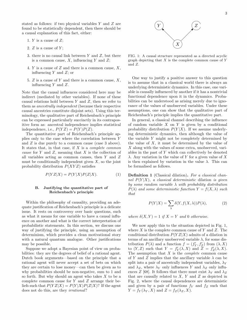
FIG. 1: A causal structure represented as a directed acyclicgraph depicting that X is the complete common cause of Yand Z.

One way to justify a positive answer to this questionis to assume that in a classical world there is always anunderlying deterministic dynamics. In this case, one vari-able is causally influenced by another if it has a nontrivialfunctional dependence upon it in the dynamics. Proba-bilities can be understood as arising merely due to igno-rance of the values of unobserved variables. Under theseassumptions, one can show that the qualitative part ofReichenbach’s principle implies the quantitative part.

In general, a classical channel describing the influenceof random variable X on Y is given by a conditionalprobability distribution P (Y |X). If we assume underly-ing deterministic dynamics, then although the value ofthe variable Y might not be completely determined bythe value of X, it must be determined by the value ofX along with the values of some extra, unobserved, vari-ables in the past of Y which can collectively be denotedλ. Any variation in the value of Y for a given value of Xis then explained by variation in the value λ. This canbe formalised as follows.

Definition 1 (Classical dilation). For a classical chan-nel P (Y |X), a classical deterministic dilation is givenby some random variable λ with probability distributionP (λ) and some deterministic function Y = f(X,λ) suchthat

P (Y |X) =∑λ

δ(Y, f(X,λ))P (λ), (2)

where δ(X,Y ) = 1 if X = Y and 0 otherwise.

We now apply this to the situation depicted in Fig. 1,where X is the complete common cause of Y and Z. Theconditional distribution P (Y Z|X) admits of a dilation interms of an ancillary unobserved variable λ, for some dis-tribution P (λ) and a function f = (f ′Y , f

′Z) from (λ,X)

to (Y,Z) such that Y = f ′Y (λ,X) and Z = f ′Z(λ,X).The assumption that X is the complete common causeof Y and Z implies that the ancillary variable λ can besplit into a pair of ancestrally independent variables, λYand λZ , where λY only influences Y and λZ only influ-ences Z [68]. It follows that there must exist λY and λZthat are causally related to X, Y and Z as depicted inFig. 2, where the causal dependences are deterministicand given by a pair of functions fY and fZ such thatY = fY (λY , X) and Z = fZ(λZ , X).

4

Z

X

Y

λY λZ

FIG. 2: The causal structure of Fig. 1, expanded so thatY and Z each has a latent variable as a causal parent inaddition to X so that both Y and Z can be made to dependfunctionally on their parents.

In this case, we have

P (Y Z|X)

=∑λY ,λZ

δ(Y, fY (λY , X))δ(Z, fZ(λZ , X))P (λY , λZ) (3)

Finally, given the qualitative part of Reichenbach’s prin-ciple, the ancestral independence of λY and λZ in thecausal structure implies that P (λY , λZ) = P (λY )P (λZ).It then follows that P (Y Z|X) = P (Y |X)P (Z|X), whichestablishes the quantitative part of Reichenbach’s princi-ple.

A well-known converse statement is also worth noting:any classical channel P (Y Z|X) satisfying P (Y Z|X) =P (Y |X)P (Z|X) admits of a dilation where X is the com-plete common cause of Y and Z [8].

Summarizing, we can identify what it means forP (Y Z|X) to be explainable in terms of X being a com-plete common cause of Y and Z by appealing to the qual-itative part of Reichenbach’s principle and fundamentaldeterminism. The definition can be formalized into amathematical condition as follows:

Definition 2 (Classical compatibility). P (Y Z|X) issaid to be compatible with X being the complete com-mon cause of Y and Z if one can find variables λY andλZ , distributions P (λY ) and P (λZ), a function fY from(λY , X) to Y and a function fZ from (λZ , X) to Z, suchthat these constitute a dilation of P (Y Z|X), that is, suchthat

P (Y Z|X)

=∑λY ,λZ

δ(Y, fY (λY , X))δ(Z, fZ(λZ , X))P (λY )P (λZ)

(4)

With this definition, we can summarize the result de-scribed above as follows.

Theorem 1. Given a conditional probability distributionP (Y Z|X), the following are equivalent:

1. P (Y Z|X) is compatible with X being the completecommon cause of Y and Z.

2. P (Y Z|X) = P (Y |Z)P (Z|X).

The 1 → 2 implication is what establishes that a ra-tional agent should espouse the quantitative part of Re-ichenbach’s principle if they espouse the qualitative partand fundamental determinism.

The 2 → 1 implication allows one to deduce a possi-ble causal explanation of an observed distribution froma feature of that distribution. However, it is importantto stress that it only establishes a possible causal expla-nation. It does not state that this is the only causal ex-planation. Indeed, it may be possible to satisfy this con-ditional independence relation within alternative causalstructures by fine-tuning the strengths of the causal de-pendences. However, as noted above, fine-tuned causalexplanations are typically rejected as bad explanations inthe field of causal inference. Therefore, the best expla-nation of the conditional independence of Y and Z givenX is that X is the complete common cause of Y and Z.

III. THE QUANTUM VERSION OFREICHENBACH’S PRINCIPLE

In this section, we introduce our quantum version ofReichenbach’s principle. The definition of a quantumcausal model that we provide in Sec. V can be seen asgeneralizing these ideas in much the same way that clas-sical causal models generalize the classical version of Re-ichenbach’s principle.

A. Quantum preliminaries

For simplicity, we assume throughout that all quantumsystems are finite-dimensional. Given a quantum systemA, we will write HA for the corresponding Hilbert space,dA for the dimension of HA, and IA for the identity onHA. We will also write H∗A for the dual space to HA,and IA∗ for the identity on the dual space. If a quantumsystem is initially uncorrelated with any other system,then the most general time evolution of the system cor-responds to a quantum channel, i.e., a completely postivetrace-preserving (CPTP) map. If the system at the ini-tial time is labelled A, with Hilbert space HA, and thesystem at the later time is labelled B, with Hilbert spaceHB , then the CPTP map is

EB|A : L(HA)→ L(HB), (5)

where L(H) is the set of linear operators on H.An alternative way to express the channel EB|A is as

an operator, using a variant of the Choi-Jamio lkowskiisomorphism [16, 17]:

ρB|A :=∑ij

EB|A(|i〉A〈j|)⊗ |i〉A∗〈j|. (6)

Here, the vectors {|i〉A} form an orthonormal basis ofthe Hilbert space HA. The vectors {|i〉A∗} form the

5

dual basis, belonging to H∗A. The operator ρB|A there-fore acts on the Hilbert space HB ⊗ H∗A. Although theexpression above involves an arbitrary choice of orthonor-mal basis, the operator ρB|A thus defined is indepen-dent of the choice of basis. This version of the Choi-Jamio lkowski isomorphism was chosen because it is bothbasis-independent and a positive operator. Following[18], we have chosen the operator ρB|A to be normalizedin such a way that TrB(ρB|A) = IA∗ (in analogy with thenormalization condition

∑Y P (Y |X) = 1 for a classical

channel P (Y |X)).Suppose that ρB = EB|A(ρA). Given that the operator

ρB|A contains all of the information about the channelEB|A, the question arises of how one can express ρB interms of ρB|A and ρA. Recall that ρB|A is defined onHB ⊗ HA∗ , while ρA is defined on HA. As we discussfurther in Sec. V, by defining an appropriate “linkingoperator” on HA := HA ⊗HA∗ ,

τ idA :=

∑lm

|l〉A∗〈m| ⊗ |l〉A〈m| (7)

where {|l〉A}l and {|l〉A∗}l are orthonormal bases onHA and HA∗ respectively, one can write ρB =TrA(ρB|Aτ

idAρA). This expression is meant to be reminis-

cent of the classical formula P (Y ) =∑Y P (Y |X)P (X).

Given an operator ρAB···|CD···, acting on HA ⊗ HB ⊗· · · ⊗ HC∗ ⊗ HD∗ ⊗ · · · , we will use the same expres-sion with missing indices to denote the result of takingpartial traces on the corresponding factor spaces. Forexample, given a channel ρAB|CD, we write ρA|CD :=TrB(ρAB|CD).

When writing products of operators, we will some-times suppress tensor products with identities. For ex-ample, (ρB|A ⊗ IC)(ρC|A ⊗ IB) will be written simply asρB|AρC|A.

B. Main result

The qualitative part of Reichenbach’s principle can beapplied to quantum theory with almost no change: ifquantum systems B and C are correlated then this musthave a causal explanation in one of the five forms listedin Sec. II A (except with classical variables X, Y and Zreplaced by quantum systems A, B and C). Here, fortwo quantum systems to be correlated means that theirjoint quantum state does not factorize.

Finding a quantum version of the quantitative partof Reichenbach’s principle is more subtle. If a quan-tum system A is a complete common cause of B andC (as depicted in Fig. 3), then one expects there to besome constraint analogous to the classical constraint thatP (Y Z|X) = P (Y |X)P (Z|X). If one tries to do this bygeneralising the joint distribution P (XY Z), then one im-mediately faces the problem that textbook quantum the-ory has no analogue of a joint distribution for a collectionof quantum systems in which some are causal descendantsof others. The situation is improved if one focusses on

C

A

B

FIG. 3: A causal structure relating three quantum systemswith A the complete common cause of B and C.

finding an analogue of P (Y Z|X) instead. In standardquantum theory, as long as a system A is initially uncor-related with its environment, then the evolution from Ato BC is described by a channel EBC|A. The operatorthat is isomorphic to this channel by Eq. (6), denotedρBC|A, seems to be a natural analogue of P (Y Z|X).However, even in this case, it is not obvious what con-straint on ρBC|A should serve as the analogue of the clas-sical constraint P (Y Z|X) = P (Y |X)P (Z|X).

The treatment of generic causal networks of quan-tum systems is deferred to the full definition of quantumcausal models in Sec. V. This section focuses on the caseof a channel ρBC|A.

In Sec. II B, we demonstrated how to justify the quan-titative part of Reichenbach’s principle from the qualita-tive part in the classical case under the assumption thatall dynamics are fundamentally deterministic. We shallnow make an analogous argument in the quantum caseby assuming that quantum dynamics are fundamentallyunitary. Just as in the classical case, this assumptionsimply provides a clean way to motivate our result andalternative justifications may be possible.

In general, a quantum channel from A to B is givenby a CPTP map EB|A. Assuming underlying unitary dy-namics, then the output state at B must depend unitarilyon A along with some extra ancillary system λ in the pastof B. This can be formalised as follows.

Definition 3 (Unitary dilation). For a quantum channelEB|A a quantum unitary dilation is given by some ancil-lary quantum system λ with state ρλ and some unitaryU from HA ⊗Hλ to HB ⊗HB such that

EB|A(·) = TrB(U(· ⊗ ρλ)U†

),

where the dimension of B is fixed by the requirement forunitarity that dAdλ = dBdB.

If we represent the channels by our variant of the Choi-Jamio lkowski isomorphism, Eq. (6), with ρB|A represent-

ing EB|A and ρUBB|Aλ representing U(·)U†, then the dila-

tion equation has the form

ρB|A = TrBλ

(ρUBB|Aλτ

idλ ρλ

)where τ id

λ is the linking operator defined in Eq. (7).Just as in the classical case, we would like to apply

this to the situation depicted in Fig. 3, where A is the

6

C

A

B

λB λC

FIG. 4: The causal structure of Fig. 3, expanded so that Band C each has a latent system as a causal parent in additionto A. By analogy the classical case, we take B and C todepend unitarily on their λB , A, and λC .

complete common cause for B and C. This was easy clas-sically as it is clear what it means for a classical variable,X, to have no causal influence on another, Y , in a deter-ministic system. Specifically, if the collection of inputsother than X is denoted X so there is a deterministicfunction f such that Y = f(X, X), then the assump-tion that X has no causal influence on Y is formalized asf(X, X) = f ′(X) for some function f ′. In unitary quan-tum theory the corresponding condition is less obvious,so we spell it out explicitly with a definition.

Definition 4 (No influence). Consider a unitary channelρUBB|AA from AA to BB. A has no causal influence on B

if and only if for ρB|AA := trBρUBB|AA, we have ρB|AA =

IA∗ ⊗ ρB|A.

An equivalent definition is this: A has no causal in-fluence on B in some unitary channel if and only if themarginal output state at B is independent of any oper-ations performed on A before the A system enters thechannel. There is a rich literature concerning similarproperties of unitary operators from various perspectives.In particular, the results of Ref. [19] are very close to ours(where they use the phrase “nonsignalling” rather than“no causal influence”) and Refs. [20, 21] contain similarresults (where they say “semi-causal” rather than “nocausal influence”).

We can now apply this to the complete common causesituation of Fig. 3. The channel EBC|A admits a uni-tary dilation in terms of an ancillary system λ, for somestate ρλ and unitary U from λA to BDC. Here, anancillary output D is generally required so that dimen-sions of inputs and outputs match, but is not importantand will always be traced out. This dilation is such thatEBC|A(·) = TrD

(U(· ⊗ ρλ)U†

).

Just as in Sec. II B, the assumption that A is a completecommon cause for B and C implies that the ancilla λcan be factorized into ancestrally independent λB andλC where λB has no causal influence on C and λC hasno causal influence on B. It follows that systems λB andλC are causally related to A, B, and C as depicted inFig. 4.

The ancestral independence of λB and λC implies thatthe quantum state on λ factorizes across the λB , λCpartition, ρλ = ρλB

ρλC, suggesting the following quan-

tum analogue to our classical compatibility condition of

Def. 2.

Definition 5 (Quantum compatibility). ρBC|A is saidto be compatible with A being a complete common causeof B and C, if it is possible to find ancillary quantumsystems λB and λC , states ρλB

and ρλC, and a unitary

channel where λB has no causal influence on C and λChas no causal influence on B, such that these constitutea dilation of ρBC|A.

All that remains is to show that this, together withthe qualitative part of the quantum Reichenbach’s prin-ciple, implies an appropriate quantitative part (general-ising Thm 1).

Theorem 2. The following are equivalent:

1. ρBC|A is compatible with A being the complete com-mon cause of B and C.

2. ρBC|A = ρB|AρC|A.

The proof is in Appendix A. Note that there is noordering ambiguity on the right-hand side of the secondcondition, because the two terms must commute. This isseen by taking the Hermitian conjugate of both sides ofthe equation and recalling that ρBC|A is Hermitian.

The strong analogy that exists between Thms 1 and 2suggests the following definition:

Definition 6 (Quantum conditional independence ofoutputs given input). Given a quantum channel ρBC|A,the outputs are said to be quantum conditionally indepen-dent given the input if and only if ρBC|A = ρB|AρC|A.

It is easily seen that the quantum definition reduces tothe classical definition in the case that the channel ρBC|Ais invariant under the operation of completely dephasingthe systems A, B, and C in some basis. More precisely: iffixed bases are chosen for HA,HB ,HC , and the operatorρBC|A is diagonal when written with respect to the ten-sor product of these bases, then the outputs are quantumconditionally independent given the input if and only ifthe classical channel defined by the diagonal elements ofthe matrix has the property that the outputs are condi-tionally independent given the input.

With this terminological convention in hand, we canexpress our quantum version of the quantitative part ofReichenbach’s principle as follows: if a channel ρBC|A iscompatible with A being a complete common cause ofB and C, then for this channel, B and C are quantumconditionally independent given A.

The 1 → 2 implication in the theorem is what estab-lishes the quantum version of the quantitative part ofReichenbach’s principle.

The 2→ 1 implication is pertinent to causal inference:analogously to the classical case, if one grants the im-plausibility of fine-tuning, then one must grant that themost plausible explanation of the quantum conditionalindependence of outputs B and C given input A is thatA is a complete common cause of B and C.

7

Thm 2, and the surrounding discussion, motivates thedefinition of quantum causal models given in Sec. V. Forthe rest of this section we make some further remarksabout the quantum version of Reichenbach’s principle.

C. Alternative expressions for quantum conditionalindependence of outputs given input

Classically, conditional independence of Y and Zgiven X is standardly expressed as P (Y Z|X) =P (Y |X)P (Z|X). However, there are alternative ways ofexpressing this constraint.

For instance, if one defines the joint distribution overX,Y, Z that one obtains by feeding the uniform dis-tribution on X into the channel P (Y Z|X)—that is,

P (XY Z) := P (Y Z|X) 1dX

, where dX is the cardinalityof X—then Y and Z being conditionally independentgiven X in P (Y Z|X) can be expressed as the vanish-ing of the conditional mutual information of Y and Zgiven X in the distribution P (XY Z) [8]. This condi-tional mutual information is defined as I(Y : Z|X) :=H(Y,X) +H(Z,X)−H(X,Y, Z)−H(X), with H(·) de-noting the Shannon entropy of the marginal on the sub-set of variables indicated in its argument. Therefore, thecondition is simply I(Y : Z|X) = 0.

Similarly, if Y and Z are conditionally independentgiven X in P (Y Z|X), then it is possible to mathemat-ically represent the channel P (Y Z|X) as the followingsequence of operations: copy X, then process one copyinto Y via the channel P (Y |X) and process the otherinto Z via the channel P (Z|X).

We present here the quantum analogues of these alter-native expressions. They will be found to be useful for de-veloping intuitions about quantum conditional indepen-dence and in proving Thm 2. Recall that the quantumconditional mutual information of B and C given A is de-fined as I(B : C|A) := S(B,A) +S(C,A)−S(A,B,C)−S(A), where S(·) denotes the von Neumann entropy ofthe reduced state on the subsystem that is specified byits argument. Analogously to the classical case, we willuse a hat to denote an operator renormalized such thatthe trace is 1. For example, if ρB|A is the operator repre-senting a channel from A to B, then ρB|A := (1/dA)ρB|A.

Theorem 3. Given a channel ρBC|A, the following con-ditions are also equivalent to the quantum conditional in-dependence of the outputs given the input (condition 2 ofThm 2):

3. I(B : C|A) = 0 where I(B : C|A) is the quantumconditional mutual information of B and C givenA evaluated on the (positive, trace-one) operatorρBC|A := (1/dA)ρBC|A.

4. The Hilbert space for the A system can be decom-posed as HA =

⊕iHAL

i⊗ HAR

iand ρBC|A =∑

i

(ρB|AL

i⊗ ρC|AR

i

), where for each i, ρB|AL

irep-

resents a CPTP map B(HALi

) → B(HB), and

ρC|ARi

a CPTP map B(HARi

)→ B(HC).

The proof is in Appendix A. That conditions 3 and 4are equivalent follows as a corollary of Thm 6 of Ref. [22].Our main contribution is showing that these are alsoequivalent to condition 2 of Thm 2.

The final condition can be described as follows. Firstone imagines decomposing the system A into a direct sumof subspaces, each of which is denoted Ai. For each i, thesubspace Ai is split into two factors, denoted ALi and ARi ,with one factor evolving via a channel ρB|AL

iinto system

B, and the other factor evolving via ρC|ARi

into system

C. In the special case where there is only a single value ofi, this is simply a factorization of the A system into twoparts. In the special case where all of the ALi and ARi are1-dimensional Hilbert spaces, it is simply an incoherentcopy operation.

D. Circuit representations

It is instructive to summarize the contents of Thms 1and 2 using circuit diagrams.

The classical case is shown in Fig. 5, where four equiv-alent circuits represent the action of a channel P (Y Z|X),for which the outputs Y Z are conditionally independentgiven the input X. The dot in the lower two circuitsrepresents a classical copy operation. Equality (1) sim-ply asserts that the conditional probability distributionP (Y Z|X) admits a classical dilation, as in Def. 1. Equal-ity (4) asserts that the channel is equivalent to a sequenceof operations in which X is copied, with one copy theinput to a channel P (Y |X) and one copy the input toa channel P (Z|X). As discussed at the beginning ofSec. III C, this is one way of expressing the fact thatY and Z are conditionally independent given X. Equal-ity (3) asserts that P (Y |X) and P (Z|X) separately ad-mit classical dilations. Finally, equality (2) asserts thatP (Y Z|X) is compatible with X being a complete com-mon cause of Y and Z by depicting conditions underwhich λY has no influence on Z and λZ has no influenceon Y .

Analogous circuit diagrams can be provided in thequantum case, as depicted in Fig. 6, with analogous in-terpretations of the various equalities. Since quantumsystems cannot be copied, however, something must re-place the dot that appears in the lower two circuits ofFig. 5. For the lower two circuits of Fig. 6, we intro-duce a new symbol that indicates the decomposition ofthe Hilbert space HA into a direct sum of tensor prod-ucts, as per condition 4 of Thm 3. The symbol is a circledecorated with the set {i}, where the value i indexes theterms in the direct sum. For each value of i, the left-handwire carries the factor HAL

iand the right-hand wire the

factor HARi

.

In the lower right circuit, the gates represent uni-tary channels, and are labelled with the corresponding

8

P(Y,Z|X)

X

P(Y|X)

X

Y

P(Z|X)

Z

X

Y Z

f

P( )

(1)

=

=

= =

(3)

(4) (2)

Y Z

P(YZ|X)

Y

P( Y)

Z

P( Z)

fY

X

Y Z

fZ

FIG. 5: Diagrammatic representation of Thm 1 and of al-ternative expressions for conditional independence of outputsgiven input (the classical analogue of Thm 3).

P(Y,Z|X)

A

A

B C

A

B C

U(1)

B C

=

=

= =

(3)

(4) (2)

B C

A

B C

BC|A

B|A C|A V W

AiAL

AiAR

AiAL

AiAR

B C

{i} {i}

i i

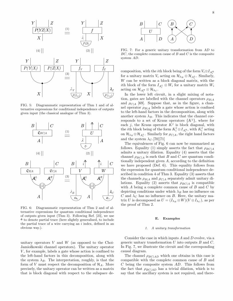
FIG. 6: Diagrammatic representation of Thm 2 and of al-ternative expressions for quantum conditional independenceof outputs given input (Thm 3). Following Ref. [23], we use

to denote partial trace (here slightly generalised, to includethe partial trace of a wire carrying an i index, defined in anobvious way.).

unitary operators V and W (as opposed to the Choi-Jamio lkowski channel operators). The unitary operatorV , for example, labels a gate whose action is confined tothe left-hand factors in this decomposition, along withthe system λB . The interpretation, roughly, is that theform of V must respect the decomposition of HA. Moreprecisely, the unitary operator can be written as a matrixthat is block diagonal with respect to the subspace de-

A D

B C

U

A D

B C

FIG. 7: For a generic unitary transformation from AD toBC, the complete common cause of B and C is the compositesystem AD.

composition, with the ith block being of the form Vi⊗IARi

for a unitary matrix Vi acting on HλB⊗HAL

i. Similarly,

W can be written as a block diagonal matrix, with theith block of the form IAL

i⊗Wi for a unitary matrix Wi

acting on HARi⊗HλC

.

In the lower left circuit, in a slight mixing of nota-tion, gates are labelled with the channel operators ρB|Aand ρC|A [69]. Suppose that, as in the figure, a chan-nel operator ρB|A labels a gate whose action is confinedto the left-hand factors in the decomposition, along withanother system λB . This indicates that the channel cor-responds to a set of Kraus operators {Kj}, where foreach j, the Kraus operator Kj is block diagonal, withthe ith block being of the form Kj

i ⊗IARi

, with Kji acting

on HλB⊗HAL

i. Similarly for ρC|A, the right hand factors

and the system λC .[70][71]The equivalences of Fig. 6 can now be summarized as

follows. Equality (1) simply asserts the fact that ρBC|Aadmits a unitary dilation. Equality (4) asserts that thechannel ρBC|A is such that B and C are quantum condi-tionally independent given A, according to the definitionwe have proposed (Def. 6). This equality follows fromthe expression for quantum conditional independence de-scribed in condition 4 of Thm 3. Equality (3) asserts thatthe channels ρB|A and ρC|A separately admit unitary di-lations. Equality (2) asserts that ρBC|A is compatiblewith A being a complete common cause of B and C bydepicting conditions under which λB has no influence onC and λC has no influence on B. Here, the unitary ma-trix U is decomposed as U = (IλB

⊗W )(V ⊗ IλC), as per

the proof of Thm 2.

E. Examples

1. A unitary transformation

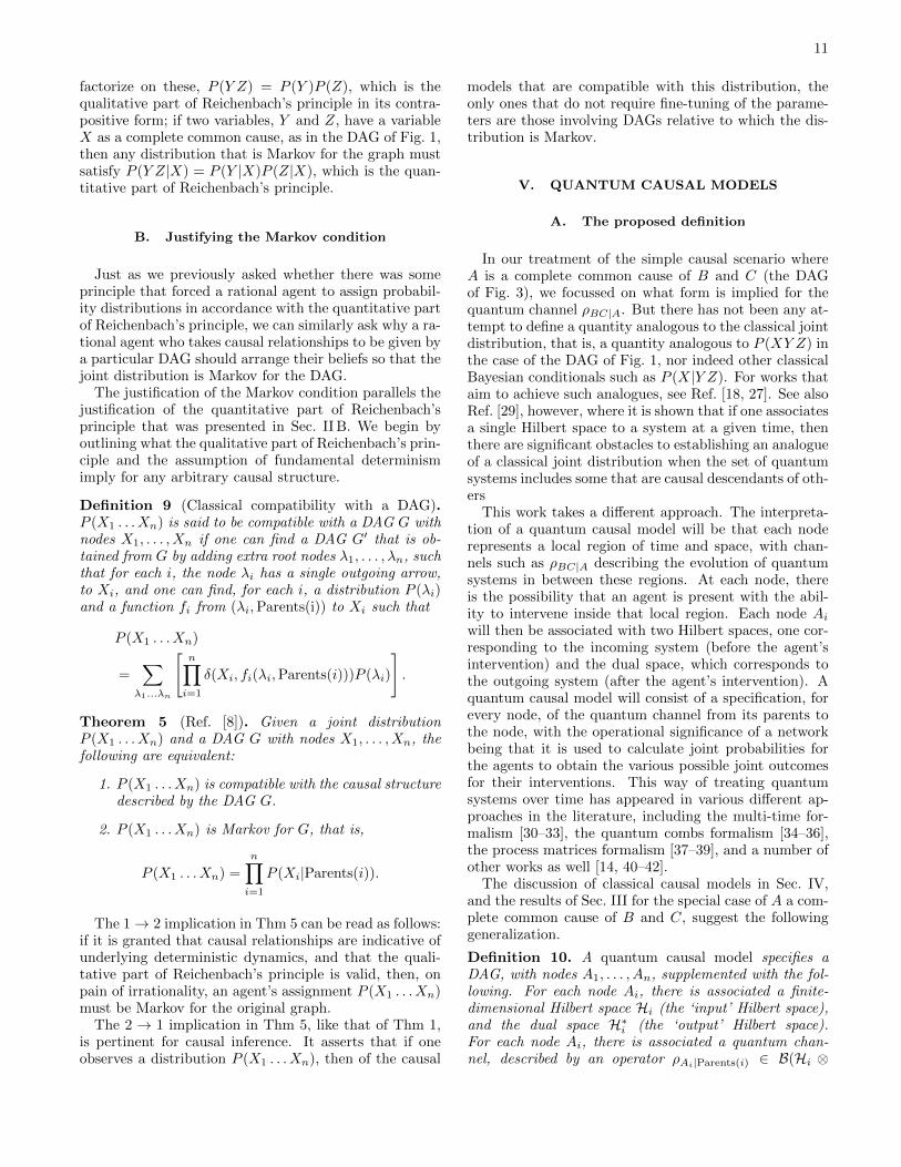
Consider the case in which inputs A andD evolve, via ageneric unitary transformation U into outputs B and C.In Fig. 7, we illustrate the circuit and the correspondingcausal diagram.

The channel ρBC|AD which one obtains in this case iscompatible with the complete common cause of B andC being the composite system AD. This follows fromthe fact that ρBC|AD has a trivial dilation, which is tosay that the ancillary system is not required, and there-

9

fore trivially satisfies the condition for compatibility laidout in Def. 5. It follows from Thm 2 that for such aρBC|AD, the outputs B and C are quantum condition-ally independent given the input AD, which means thatρBC|AD = ρB|ADρC|AD, as can also be verified by directcalculation. Similarly, the alternative expressions for thissort of quantum conditional independence, namely, con-ditions 3 and 4 of Thm 3, can be verified to hold.

2. Coherent copy vs. incoherent copy

Consider the simple example of a classical channel, tak-ing X to Y,Z, where X,Y, Z are bit-valued and the map-ping between input strings and output strings is

0X → 0Y 0Z ,

1X → 1Y 1Z . (8)

The outputs of the channel are conditionally independentgiven the input; variation in X fully explains any correla-tion between Y and Z. Indeed this example may be seenas the paradigmatic case of the explanation of classicalcorrelations via a complete common cause.

One quantum analogue of this channel is the incoher-ent copy of a qubit: a qubit A is measured in the com-putational basis; if 0 is obtained, then prepare the state|00〉BC and if 1 is obtained, prepare |11〉BC . The opera-tor representing this channel is

ρBC|A = |000〉〈000|BCA∗ + |111〉〈111|BCA∗ .

It is easily verified that this operator satisfies each ofthe conditions of Thm 2, so that B and C are quantumconditionally independent given A for this channel. Thedecomposition of the A Hilbert space implied by Condi-tion 4 is

HA = (C⊗ C)⊕ (C⊗ C) ,

where C is the 1-dimensional complex Hilbert space, i.e.,the complex numbers.

The other direct quantum analogue of the classicalcopy above is the channel that makes a coherent copyof a qubit, where the mapping from input states to out-put states is:

α|0〉A + β|1〉A → α|0〉B |0〉C + β|1〉B |1〉C . (9)

This channel is represented by the operator

ρBC|A = (|000〉BCA∗+|111〉BCA∗)(〈000|BCA∗+〈111|BCA∗),

which corresponds to an unnormalized GHZ state. Itcan easily be verified that I(B : C|A) = 1 for a trace-oneversion of this state, hence it is not the case that outputsB and C are quantum conditionally independent giventhe input A. There is, then, no way in which this channelcan arise as a marginal channel in a situation in which Ais the complete common cause of B and C.

λX

Y Z

δ(λ,0)X

Y Z

λ

FIG. 8: Classical realization of a copy operation using anancilla and classical CNOT gate.

λA

B C

A

B C

λ

|0⟩λ⟨0|

FIG. 9: Quantum realization of the coherent copy using anancilla and quantum CNOT gate.

At first blush, this conclusion may seem surprising.Given the mapping described by Eq. (9), where wouldcorrelations between outputs B and C come from, otherthan being completely explained by the input A?

The puzzle is resolved by considering the dilation ofthe coherent copy to a unitary transformation, and theinterpretation of quantum pure states. Consider Figs. 8and 9, which respectively show a classical copy operationvia the classical CNOT gate and a quantum coherentcopy operation via the quantum CNOT gate [72].

In the classical case, there are two reasons why anycorrelation between Y and Z must be entirely explainedby statistical variation in the value of X. First, the ancil-lary variable λ is prepared deterministically with value 0,so there is no possibility that statistical variation in thevalue of λ underwrites the correlations between B and C.Second, the mapping between input strings and outputstrings for the classical CNOT gate,

0X0λ → 0Y 0Z ,

0X1λ → 0Y 1Z ,

1X0λ → 1Y 1Z ,

1X1λ → 1Y 0Z , (10)

(which one easily verifies to reduce to the classical copyof Eq. (8) when one sets λ to 0), has the causal structuredepicted in Fig. 8, so that λ does not act as a commoncause of Y and Z but only a local cause of Z.

In the quantum case, neither reason applies. Concern-ing the second reason, the quantum CNOT has the causalstructure depicted in Fig. 9: the quantum CNOT is suchthat not only does A have a causal influence on C, butλ has a causal influence on B as well. In other words,unlike the classical CNOT, there is a back action of thetarget on the control. It follows that in the quantumcase, λ can act as a common cause of B and C. Further-more, the ancilla is prepared in a quantum pure state|0〉. This is dis-analogous to a point distribution on the

10

value 0 for the classical variable λ if one takes the viewthat a quantum pure state represents maximal but in-complete information about a quantum system [24–28].In this case, one must allow for the possibility that somecorrelation between B and C is due to the ancilla, inwhich case A is not the complete common cause of Band C [73].

F. Generalization to one input, k outputs

Thms 2 and 3, which apply to quantum channels withone input and two outputs, can be generalized to the caseof one input and k outputs.

Consider a channel ρB1...Bk|A, and let Bi denote thecollection of all outputs apart from Bi. The notion ofquantum compatibility from Def. 5 generalizes in the ob-vious way: ρB1...Bk|A is said to be compatible with Abeing a complete common cause of B1 . . . Bk, if it is pos-sible to find ancillary quantum systems λ1, . . . , λk, statesρλ1 , . . . , ρλk

, and a unitary channel where, for each i, λihas no causal influence on Bi, such that these constitutea dilation of ρB1...Bk|A.

The generalization of Thms 2 and 3, consolidated intoa single theorem, is as follows:

Theorem 4. The following are equivalent:

1. ρB1...Bk|A is compatible with A being a completecommon cause of B1 . . . Bk.

2. ρB1...Bk|A = ρB1|A · · · ρBk|A, where for all i, j,[ρBi|A, ρBj |A] = 0.

3. For each i, I(Bi : Bi|A) = 0 where I(Bi : Bi|A) isthe quantum conditional mutual information evalu-ated on the (positive, trace-one) operator ρB1...Bk|A.

4. The Hilbert space for the A system can be decom-posed as HA =

⊕iHA1

i⊗ · · · ⊗ HAk

isuch that

ρB1...Bk|A =∑i

(ρB1|A1

i⊗ · · · ⊗ ρBk|Ak

i

), where for

each i, and each l ∈ {1, . . . , k}, ρB|Ali

represents a

CPTP map B(HAli)→ B(HBl

).

The proof is in Appendix B. By analogy to the classicalcase, if conditions 2, 3 and 4 of Thm 4 hold, we say thatB1 . . . Bk are quantum conditionally independent givenA for the channel ρB1...Bk|A.

IV. CLASSICAL CAUSAL MODELS

A. Definitions

Reichenbach’s principle is important because it gener-alizes to the modern formalism of causal models [8, 9].

A causal model consists of two entities: (i) a causalstructure, represented by a directed acyclic graph (DAG)where the nodes represent random variables and thedirected edges represent the directed causal influencesamong these (several examples have already been pre-sented in this article), and (ii) some parameters, whichspecify the strength of the causal dependences and theprobability distributions for the variables associated toroot nodes in the DAG (i.e., those with no incoming ar-rows). Some terminology is required to present the for-mal definitions.

Given a DAG with nodes X1, . . . , Xn, let Parents(i)denote the parents of node Xi, that is, the set of nodesthat have an arrow into Xi, and let Children(i) denotethe children of node Xi, that is, the set of nodes Xj suchthat there is an arrow from Xi to Xj . The descendentsof Xi are those nodes Xj , j 6= i, such that there is adirected path from Xi to Xj . The ancestors of Xi arethose nodes Xj such that Xi is a descendent of Xj .

Definition 7. A causal model specifies a DAG, withnodes corresponding to random variables X1, . . . , Xn,and a family of conditional probability distributions{P (Xi|Parents(i))}, one for each i.

Definition 8. Given a DAG, with random variablesX1, . . . , Xn for nodes, and given an arbitrary joint dis-tribution P (X1 . . . Xn), the distribution is said to beMarkov for the graph if and only if it can be writtenin the form of

P (X1 . . . Xn) =

n∏i=1

P (Xi|Parents(i)). (11)

(Recall that each conditional P (Xi|Parents(i)) can becomputed from the joint P (X1 . . . Xn).)

The generalization of Reichenbach’s principle that isafforded by the formalism of causal models is this: if thereare statistical dependences among variables X1, . . . , Xn,expressed in the particular form of the joint distributionP (X1 . . . Xn), then there should be a causal explanationof these dependences in terms of a DAG relative to whichthe distribution P (X1 . . . Xn) is Markov.

Note that an alternative way of formalizing theMarkov property is that P (X1 . . . Xn) is Markov for thegraph if and only if, for each i, P (Xi|Parents(i)) =P (Xi|Nondesc(i)), where Nondesc(i) is the set of non-descendents of node Xi. The intuitive idea is that theparents of a node screen off that node from the othernondescendents: once the values of the parents are fixed,the values of other non-descendent nodes are irrelevantto the value of Xi.

Note also that Reichenbach’s principle is easily seento be a special case of the requirement that for a jointdistribution to be explainable by the causal structure ofsome DAG, it must be Markov for that DAG: if two vari-ables, Y and Z, are ancestrally independent in the graph,then any distribution that is Markov for this graph must

11

factorize on these, P (Y Z) = P (Y )P (Z), which is thequalitative part of Reichenbach’s principle in its contra-positive form; if two variables, Y and Z, have a variableX as a complete common cause, as in the DAG of Fig. 1,then any distribution that is Markov for the graph mustsatisfy P (Y Z|X) = P (Y |X)P (Z|X), which is the quan-titative part of Reichenbach’s principle.

B. Justifying the Markov condition

Just as we previously asked whether there was someprinciple that forced a rational agent to assign probabil-ity distributions in accordance with the quantitative partof Reichenbach’s principle, we can similarly ask why a ra-tional agent who takes causal relationships to be given bya particular DAG should arrange their beliefs so that thejoint distribution is Markov for the DAG.

The justification of the Markov condition parallels thejustification of the quantitative part of Reichenbach’sprinciple that was presented in Sec. II B. We begin byoutlining what the qualitative part of Reichenbach’s prin-ciple and the assumption of fundamental determinismimply for any arbitrary causal structure.

Definition 9 (Classical compatibility with a DAG).P (X1 . . . Xn) is said to be compatible with a DAG G withnodes X1, . . . , Xn if one can find a DAG G′ that is ob-tained from G by adding extra root nodes λ1, . . . , λn, suchthat for each i, the node λi has a single outgoing arrow,to Xi, and one can find, for each i, a distribution P (λi)and a function fi from (λi,Parents(i)) to Xi such that

P (X1 . . . Xn)

=∑

λ1...λn

[n∏i=1

δ(Xi, fi(λi,Parents(i)))P (λi)

].

Theorem 5 (Ref. [8]). Given a joint distributionP (X1 . . . Xn) and a DAG G with nodes X1, . . . , Xn, thefollowing are equivalent:

1. P (X1 . . . Xn) is compatible with the causal structuredescribed by the DAG G.

2. P (X1 . . . Xn) is Markov for G, that is,

P (X1 . . . Xn) =

n∏i=1

P (Xi|Parents(i)).

The 1→ 2 implication in Thm 5 can be read as follows:if it is granted that causal relationships are indicative ofunderlying deterministic dynamics, and that the quali-tative part of Reichenbach’s principle is valid, then, onpain of irrationality, an agent’s assignment P (X1 . . . Xn)must be Markov for the original graph.

The 2 → 1 implication in Thm 5, like that of Thm 1,is pertinent for causal inference. It asserts that if oneobserves a distribution P (X1 . . . Xn), then of the causal

models that are compatible with this distribution, theonly ones that do not require fine-tuning of the parame-ters are those involving DAGs relative to which the dis-tribution is Markov.

V. QUANTUM CAUSAL MODELS

A. The proposed definition

In our treatment of the simple causal scenario whereA is a complete common cause of B and C (the DAGof Fig. 3), we focussed on what form is implied for thequantum channel ρBC|A. But there has not been any at-tempt to define a quantity analogous to the classical jointdistribution, that is, a quantity analogous to P (XY Z) inthe case of the DAG of Fig. 1, nor indeed other classicalBayesian conditionals such as P (X|Y Z). For works thataim to achieve such analogues, see Ref. [18, 27]. See alsoRef. [29], however, where it is shown that if one associatesa single Hilbert space to a system at a given time, thenthere are significant obstacles to establishing an analogueof a classical joint distribution when the set of quantumsystems includes some that are causal descendants of oth-ers

This work takes a different approach. The interpreta-tion of a quantum causal model will be that each noderepresents a local region of time and space, with chan-nels such as ρBC|A describing the evolution of quantumsystems in between these regions. At each node, thereis the possibility that an agent is present with the abil-ity to intervene inside that local region. Each node Aiwill then be associated with two Hilbert spaces, one cor-responding to the incoming system (before the agent’sintervention) and the dual space, which corresponds tothe outgoing system (after the agent’s intervention). Aquantum causal model will consist of a specification, forevery node, of the quantum channel from its parents tothe node, with the operational significance of a networkbeing that it is used to calculate joint probabilities forthe agents to obtain the various possible joint outcomesfor their interventions. This way of treating quantumsystems over time has appeared in various different ap-proaches in the literature, including the multi-time for-malism [30–33], the quantum combs formalism [34–36],the process matrices formalism [37–39], and a number ofother works as well [14, 40–42].

The discussion of classical causal models in Sec. IV,and the results of Sec. III for the special case of A a com-plete common cause of B and C, suggest the followinggeneralization.

Definition 10. A quantum causal model specifies aDAG, with nodes A1, . . . , An, supplemented with the fol-lowing. For each node Ai, there is associated a finite-dimensional Hilbert space Hi (the ‘input’ Hilbert space),and the dual space H∗i (the ‘output’ Hilbert space).For each node Ai, there is associated a quantum chan-nel, described by an operator ρAi|Parents(i) ∈ B(Hi ⊗

12

H∗Parents(i)), where H∗Parents(i) is the tensor product of

the output Hilbert spaces associated with the parents ofAi. These channels commute pairwise, i.e., for anyi, j, [ρAi|Parents(i), ρAj |Parents(j)] = 0 (which is a non-trivial constraint whenever Parents(i) ∩ Parents(j) isnonempty). The overall state is respresented by an op-erator on

⊗ni=1HAi , where HAi := HAi ⊗H∗Ai

, denotedσA1...An

and given by

σA1...An=

n∏i=1

ρAi|Parents(i). (12)

Recall from Section III that, given a quantum channelρBC|A, it is compatible with A being the complete com-mon cause of B and C if and only if ρBC|A = ρB|AρC|A,and if this holds, then [ρB|A, ρC|A] = 0. The definitionof a quantum causal model, in particular, the stipula-tion that the channels commute pairwise, generalizes thisidea.

B. Making predictions

In order to see how a quantum causal model is used tocalculate probabilities for the outcomes of agents’ inter-ventions, consider a quantum causal model with nodesA1, . . . , An and state σA1...An

. Let the intervention atnode Ai have classical outcomes labelled by ki. The inter-vention is defined by a quantum instrument (that is, bya set of completely-positive trace-non-increasing maps,one for each outcome) which sum to a trace-preservingmap. In order to write the probabilities for the outcomesin a simple form, it is useful to define the instrumentin such a way that the map associated to each outcometakes operators on H∗Ai

into operators on H∗Ai. Hence,

suppose that the outcome ki corresponds to the mapEkiAi

: B(H∗Ai)→ B(H∗Ai

) and let

τkiAi=∑lm

EkiAi(|l〉A∗

i〈m|)⊗ |l〉Ai

〈m|.

The outcome ki of the agent’s intervention can then berepresented by the (positive, basis-independent) operator

τkiAiisomorphic to EkiAi

.If an agent does not intervene at the node Ai, this

corresponds to the linking operator itself,

τ idAi

=∑lm

|l〉A∗i〈m| ⊗ |l〉Ai

〈m|.

The joint probability for the agents to obtain outcomesk1, . . . , kn is given by

P (k1 . . . kn) = Tr(σA1...An(τk1A1

⊗ · · · ⊗ τknAn)). (13)

We can also define operations on the state σA1...Ancor-

responding to marginalization over the outcome ki of anintervention on node Ai by

∑ki

TrAi. In this case, the

joint state on the rest of the nodes after such marginal-ization is

σA1...A(i−1)A(i+1)...An =∑ki

TrAi(σA1...AnτkiAi

).

If the intervention at node Ai is trivial, then

σA1...A(i−1)A(i+1)...An = TrAi(σA1...AnτidAi

).

C. Classical interventional models

Given the proposed definition of a quantum causalmodel, and the interpretation in terms of agents inter-vening at nodes, there is a stronger analogy to be madewith a classical formalism that similarly involves inter-ventions, than there is to the standard classical causalmodels introduced in Sec. IV.

In order to make this explicit, consider a classical in-terventional causal model constructed as follows. For agiven DAG, split every node Xi into a pair of discon-nected nodes, denoted XO

i and XIi , such that in the

DAG that results, XIi has as parents the set of nodes

ParentsO(i) := {XOj : Xj ∈ Parents(i)}, and XO

i has as

children {XIj : Xj ∈ Chidren(i)}. In other words, the ‘I’

version of each node Xi has as parents the ‘O’ version ofeach node that was a parent of Xi in the original graph,and the ‘O’ version of each node Xi has as children the‘I’ version of each node that was a child of Xi in the orig-inal graph. In this case, one can represent the resultingDAG by a conditional probability distribution

P (XI1 . . . X

In|XO

1 . . . XOn ) =

n∏i=1

P (XIi |ParentsO(i)).

(14)

Our association of each node Ai of the DAG with a pairof Hilbert spaces, HAi

andH∗Ai, is simply a quantum ver-

sion of the splitting of a classical variable Xi into XOi and

XIi , and our joint state σA1...An is the quantum analogue

of the conditional probability P (XI1 . . . X

In|XO

1 . . . XOn ).

In a classical interventional causal model, one canimagine an intervention at node Xi as a causal processacting between XI

i and XOi and possibly outputing an

additional classical variable ki which acts as a record ofsome aspect of the intervention. The most general suchintervention is described by a conditional probability dis-tribution P (ki, X

Oi |XI

i ) [74]. After specifying the natureof the intervention at each node, {P (ki, X

Oi |XI

i )}i, onecan compute the joint probability distribution over therecord variables to be

P (k1 . . . kn) =∑

XI1 ,X

O1 ...X

In,X

On

P (XI1 . . . X

In|XO

1 . . . XOn )

×n∏i=1

P (ki, XOi |XI

i ). (15)

13

C

A

B

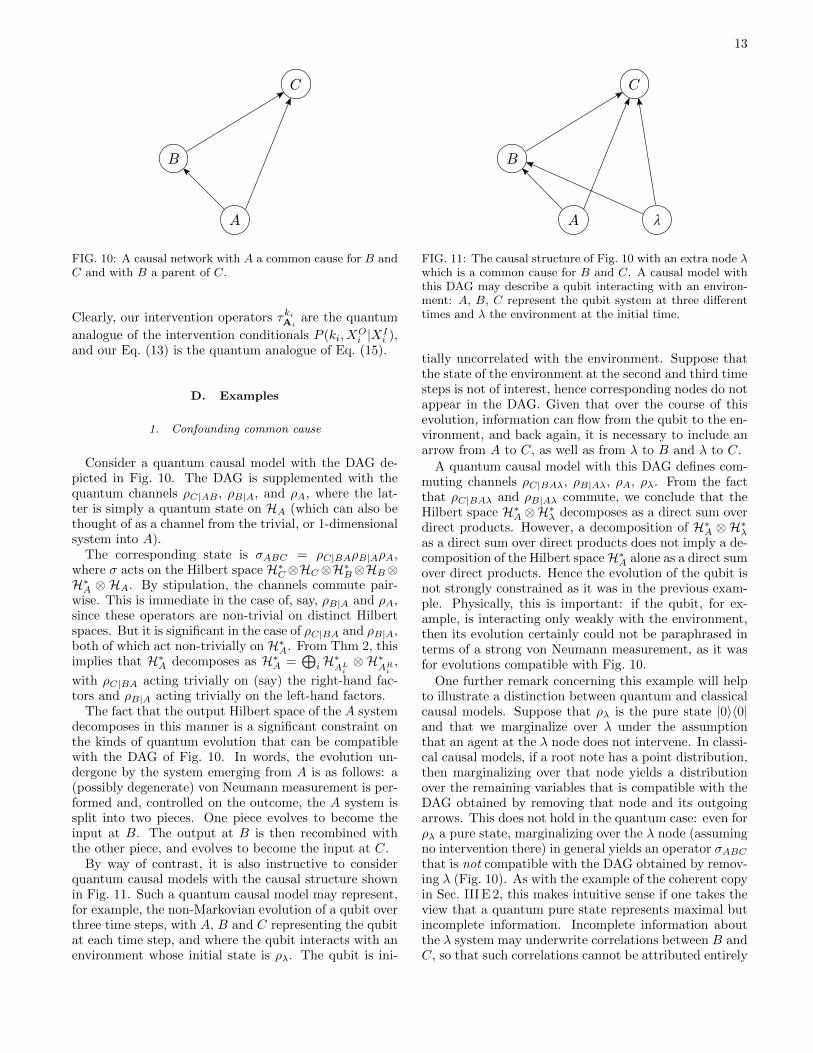
FIG. 10: A causal network with A a common cause for B andC and with B a parent of C.

Clearly, our intervention operators τkiAiare the quantum

analogue of the intervention conditionals P (ki, XOi |XI

i ),and our Eq. (13) is the quantum analogue of Eq. (15).

D. Examples

1. Confounding common cause

Consider a quantum causal model with the DAG de-picted in Fig. 10. The DAG is supplemented with thequantum channels ρC|AB , ρB|A, and ρA, where the lat-ter is simply a quantum state on HA (which can also bethought of as a channel from the trivial, or 1-dimensionalsystem into A).

The corresponding state is σABC = ρC|BAρB|AρA,where σ acts on the Hilbert space H∗C⊗HC⊗H∗B⊗HB⊗H∗A ⊗ HA. By stipulation, the channels commute pair-wise. This is immediate in the case of, say, ρB|A and ρA,since these operators are non-trivial on distinct Hilbertspaces. But it is significant in the case of ρC|BA and ρB|A,both of which act non-trivially on H∗A. From Thm 2, thisimplies that H∗A decomposes as H∗A =

⊕iH∗AL

i⊗ H∗

ARi

,

with ρC|BA acting trivially on (say) the right-hand fac-tors and ρB|A acting trivially on the left-hand factors.

The fact that the output Hilbert space of the A systemdecomposes in this manner is a significant constraint onthe kinds of quantum evolution that can be compatiblewith the DAG of Fig. 10. In words, the evolution un-dergone by the system emerging from A is as follows: a(possibly degenerate) von Neumann measurement is per-formed and, controlled on the outcome, the A system issplit into two pieces. One piece evolves to become theinput at B. The output at B is then recombined withthe other piece, and evolves to become the input at C.

By way of contrast, it is also instructive to considerquantum causal models with the causal structure shownin Fig. 11. Such a quantum causal model may represent,for example, the non-Markovian evolution of a qubit overthree time steps, with A, B and C representing the qubitat each time step, and where the qubit interacts with anenvironment whose initial state is ρλ. The qubit is ini-

λ

C

A

B

FIG. 11: The causal structure of Fig. 10 with an extra node λwhich is a common cause for B and C. A causal model withthis DAG may describe a qubit interacting with an environ-ment: A, B, C represent the qubit system at three differenttimes and λ the environment at the initial time.

tially uncorrelated with the environment. Suppose thatthe state of the environment at the second and third timesteps is not of interest, hence corresponding nodes do notappear in the DAG. Given that over the course of thisevolution, information can flow from the qubit to the en-vironment, and back again, it is necessary to include anarrow from A to C, as well as from λ to B and λ to C.

A quantum causal model with this DAG defines com-muting channels ρC|BAλ, ρB|Aλ, ρA, ρλ. From the factthat ρC|BAλ and ρB|Aλ commute, we conclude that theHilbert space H∗A ⊗H∗λ decomposes as a direct sum overdirect products. However, a decomposition of H∗A ⊗H∗λas a direct sum over direct products does not imply a de-composition of the Hilbert spaceH∗A alone as a direct sumover direct products. Hence the evolution of the qubit isnot strongly constrained as it was in the previous exam-ple. Physically, this is important: if the qubit, for ex-ample, is interacting only weakly with the environment,then its evolution certainly could not be paraphrased interms of a strong von Neumann measurement, as it wasfor evolutions compatible with Fig. 10.

One further remark concerning this example will helpto illustrate a distinction between quantum and classicalcausal models. Suppose that ρλ is the pure state |0〉〈0|and that we marginalize over λ under the assumptionthat an agent at the λ node does not intervene. In classi-cal causal models, if a root note has a point distribution,then marginalizing over that node yields a distributionover the remaining variables that is compatible with theDAG obtained by removing that node and its outgoingarrows. This does not hold in the quantum case: even forρλ a pure state, marginalizing over the λ node (assumingno intervention there) in general yields an operator σABCthat is not compatible with the DAG obtained by remov-ing λ (Fig. 10). As with the example of the coherent copyin Sec. III E 2, this makes intuitive sense if one takes theview that a quantum pure state represents maximal butincomplete information. Incomplete information aboutthe λ system may underwrite correlations between B andC, so that such correlations cannot be attributed entirely

14

to system A as Fig. 10 requires. Hence, even for the en-vironment initially in a pure state, the non-Markovianevolution of a qubit need not obey the strong constraintimplied by the causal structure of Fig. 10.

2. A simple case of Bayesian updating

This section discusses another sense in which the quan-tum notion of conditional independence of the outputs ofa channel given the input mirrors qualitatively an impor-tant aspect of the classical case.

Consider a classical causal model with the DAG ofFig. 1 and distribution P (XY Z) such that P (Y Z|X) =P (Y |X)P (Z|X). A particular feature of this causal sce-nario is that if new information is obtained about thevariable Y , for example, if an agent learns that the valueof Y is y, then the process of Bayesian updating pro-ceeds as follows. First, update the distribution over Xby applying the rule

P (X) := P (X|Y = y) =P (Y = y|X)P (X)

P (Y = y).

Then use the new probability distribution on X, P (X),to get an updated distribution for Z:

P (Z|Y = y) =∑x

P (Z|X)P (X), (16)

where the sum ranges over the values that X may take.Roughly speaking, the process of Bayesian updating “fol-lows the arrows” of the graph. For this it is crucialthat the joint distribution P (XY Z) satisfies P (Y Z|X) =P (Y |X)P (Z|X), otherwise the term P (Z|X) in Eq. (16)would have to be replaced with P (Z|X,Y = y).

Consider now a quantum causal model, with the DAGof Fig. 3 and with state σABC = ρB|AρC|AρA. Supposethat an agent at B intervenes, obtaining outcome kB ,corresponding to the operator τkBB . The agent wishes tocalculate the probability that an intervention at C yieldsoutcome kC corresponding to τkCC , conditioned on havingobtained the outcome kB , and assuming that there is nointervention at A. This can be done as follows. First,update the state assigned to A given the knowledge ofkB to

σA := σA|kB =TrB(σABτ

kBB )

Tr(σAB(τ idA ⊗ τ

kBB ))

.

Then apply the channel ρC|A to σA to get the state as-signed to C given the knowledge of kB :

σC|kB = TrA(ρC|AσAτidA ).

Finally, calculate the probability of kC :

P (kC |kB) = Tr(σC|kBτkCC ).

Again, the process of Bayesian updating “follows the ar-rows” of the graph. Note that for this to work, it was cru-cial that the channel ρBC|A satisfied ρBC|A = ρB|AρC|A.

VI. RELATION TO PRIOR WORK

We now present a short review of prior works on quan-tum causal models and describe how our own proposalrelates to these.

Preliminary work in this area took to form of ex-plorations of Bell-type inequalities (and whether theyadmit of quantum violations) for novel causal scenar-ios [43, 44]. Several researchers recognized that the for-malism of classical causal models could provide a unify-ing framework in which to pose the problem of derivingBell-type constraints, and that this framework might beextended to address the problem of deriving constraintson the correlations that can be obtained with quantumresources [2, 10, 11, 45]. Note that such constraintsare expressed entirely in terms of classical settings andclassical outcomes of measurements. Henson, Lal andPusey [46] and Fritz [47] independently proposed defi-nitions of quantum causal models with the purpose ofexpressing such constraints. In these approaches, eachnode of the DAG represents a process (which may havea classical outcome), while each directed edge is asso-ciated with a system that is passed between processes.However, despite the fact that their frameworks incor-porate the possibility of post-classical resources, they donot have sufficient structure to define conditional inde-pendences between quantum systems.

Operational reformulations of quantum theory such asRefs. [48–53] helped to set the stage for the developmentof quantum causal models. Although they were conceivedindependently of the framework of classical causal mod-els, they were quite similar to that framework insofar asthey made heavy use of DAGs—in the form of circuitdiagrams—to depict structural features of a set of pro-cesses. When the authors of these formulations turnedtheir attention to relativistic causal structure, the frame-works they devised drew even closer in spirit to that ofcausal models. Prominent examples include: the causa-loid framework of Hardy [54], the multi-time formalismof Aharonov and co-workers [30–33], the quantum combsframework of Chiribella, D’Ariano and Perinotti [34–36], the causal categories of Coecke and Lal [23], andthe process matrix formalism of Oreshkov, Costa andBrukner [37, 38]. A common aim of these approachesis to be able to compute the consequences of an inter-vention upon a particular quantum system within thecircuit, and this is precisely one of the tasks that a quan-tum analogue of a causal model should be able to handle.

Many of these frameworks represent a quantum systemat a given region of space-time by two copies of its Hilbertspace, one corresponding to the system that is input intothe region and one corresponding to the system that isoutput from it. In this way, the region becomes a “locusof intervention” for the system. By inserting a particu-lar quantum process into the “slot”, one determines thenature of the intervention. This is the approach taken,for instance, in the multi-time formalism of Ref. [31],the quantum combs of Ref. [34], and the process matri-

15

ces of Ref. [37]. This representation of interventions hasa counterpart in classical causal models, for instance inthe work of [55], as was noted in Refs. [14, 39].

Costa and Shrapnel [39] in particular have sought toexplicitly cast this sort of framework as a quantum gener-alization of a causal model. In their approach, the nodesof the DAG are associated with a quantum system lo-calized in a region (understood as a potential locus ofintervention) and the collection of edges from one set ofnodes to another represent causal processes.

An approach of this sort is required if one seeks to findintrinsically quantum versions of important theorems ofclassical causal models. For instance, while Henson, Laland Pusey [46] derive a generalization of the d-separationtheorem of classical causal models, it only infers condi-tional independence relations from d-separation relationsfor the classical variables in the graph. An intrinsicallyquantum version of the d-separation theorem, by con-trast, would be one which concerns the causal relationsamong quantum systems (see, for instance, [56]). If a setof nodes representing quantum systems can be describedby a joint or conditional state, then one can seek to de-termine whether factorization conditions on this stateare implied by d-separation relations among the quan-tum systems on the graph. Similarly, while both the ap-proaches of Henson, Lal and Pusey [46] and of Fritz [47]allow one to derive, from the structure of the DAG, con-straints on the joint distribution over classical variablesembedded therein, they do not address an intrinsicallyquantum version of this problem. If a set of nodes repre-senting quantum systems can be described by a joint orconditional state, then one can seek to derive constraintson this state directly from the structure of the DAG.

Our own approach aims at an intrinsically quantumgeneralization of the notion of a causal model. We there-fore associate to each node of the DAG a quantum systemlocalized to a space-time region, and we represent it bya pair of Hilbert spaces, corresponding to the input andoutput of an intervntion upon the system. Consequently,our approach is very similar to that of Costa and Shrap-nel [39]. Nonetheless, there is a significant difference inhow we represent common causes.

In Costa and Shrapnel’s work, any node with multipleoutgoing edges is represented as a locus of interventionwhere the output Hilbert space is a tensor product ofHilbert spaces, one for each outgoing edge. As such, anynode acting as a common cause must be associated witha composite quantum system. It cannot, for instance,be associated with a single qubit. By contrast, our ap-proach does not constrain the representation of commoncauses in this fashion. Any quantum system, includinga single qubit, may constitute a complete common causeof a collection of other quantum systems. This extragenerality is required since, as our examples have shown,the complete common cause of a set of systems can bea single qubit. Second, and more importantly, our workhas shown that for a quantum channel whose input isthe complete common cause of its n outputs, it is not

the case that the channel must split the input into ncomponents, each of which exerts a causal influence ona different output. This is merely one special case of themost general form that such a channel can take. Third,if the complete common causes consist of multiple nodesin the DAG, then it is only the joint Hilbert space ofthe collection of these that must satisfy the conditionof factorizing-in-subspaces, while each individual Hilbertspace need not.

These differences are likely to have a significant impacton the form of any intrinsically quantum d-separationtheorem.

Finally, we mention a third purpose to which quan-tum causal models can be put. Theorems about classicalcausal models often concern the sorts of inferences onecan make about one variable given information aboutanother. As an example, if Z is a common effect of Xand Y , then learning Z can induce correlations betweenX and Y . As such, one might expect quantum causalmodels to also constrain the sort of inferences one canmake among quantum variables. Early work by Leiferand Spekkens [18] had this purpose in mind. The authorsnoted various scenarios in which their proposal could notbe applied, and subsequent work [29] has narrowed downthe scope of possibilities for any such proposal. Ourown proposal provides the means of making many of theBayesian inferences considered in Ref. [18]. The case dis-cussed in Sec. V D 2 is one such example.

There is also prior work on quantum causal modelsthat takes a significantly different approach to the onesdescribed above and for which the relation to our workis less clear. The work of Tucci [57, 58], which is in factthe earliest attempt at a quantum generalization of acausal model, represents causal dependences by complextransition amplitudes rather than quantum channels.

VII. CONCLUSIONS

The field of classical statistics has benefited greatlyfrom analysis provided by the formalism of causal mod-els [8, 9]. In particular, this formalism allows one to inferfacts about the underlying causal structure purely fromuncontrolled statistical data, a tool with significant appli-cations in all branches of the physical and social sciences.Given that some seemingly paradoxical features of clas-sical correlations have found satisfying resolutions whenviewed through a causal lens, one might wonder to whatextent the same is true of quantum correlations.

Starting with the idea that whatever innovation quan-tum theory might hold for causal models, the intuitioncontained in Reichenbach’s principle ought to be pre-served, we motivated the problem of finding a quantumversion of the principle. This required us to determinewhat constraint a channel from A to BC must satisfyif A is the complete common cause of B and C. Wesolved the problem by considering a unitary dilation ofthe channel and by noting that there is no ambiguity

16

in how to represent the absence of causal influences be-tween certain inputs and certain outputs of a unitary.From this, we derived a notion of quantum conditionalindependence for the outputs of the channel given its in-put. This inference from a common-cause structure toquantum conditional independence was then generalizedto obtain our quantum version of causal models.

Given a state on a quantum causal model, we describedhow to construct a marginal state for a subset of nodes.We discussed a number of simple examples of quantumchannels and causal structures. A theme of the exam-ples is that when there is a difference between the quan-tum and classical cases, this can often be understood ifone takes the view that a quantum pure state representsmaximal but incomplete information about a system, andhence may underwrite correlations between other systemsin a way that a classical pure state cannot.

There are many directions for future work. In the caseof classical causal networks, an important theorem statesthat the d-separation relation among nodes of a DAG issound and complete for a conditional independence rela-tion to hold among the associated variables in the jointprobability distribution [8]. Here, for arbitrary subsetsof nodes S, T and U , subsets S and T are said to bed-separated by U if a certain criterion holds, where thisis determined purely by the structure of the DAG. Animportant question is therefore whether d-separation issound and complete for some natural property of thestate σ on a quantum causal network.

It is also desirable to relate properties of a quantumcausal network to operational statements involving theoutcomes of agents’ interventions: under what circum-stances, for example, does it follow that there is an inter-vention by the agents at nodes in a subset U , such that,conditioned on its outcome, the outcomes of any inter-ventions by agents at S and T must be independent?Such a result would have an application to quantum pro-tocols. Imagine, for example, a cryptographic scenario inwhich agents at S and T desire shared correlations thatare not screened off by the information held by agents atU .

In the classical case, there has been a great deal ofwork on the problem of causal inference [8, 59–61]: givenonly certain facts about the joint probabilities, for in-stance, a set of conditional independences, what canbe inferred about the underlying causal structure? Foran initial approach to quantum causal inference, with aquantum-over-classical advantage in a simple scenario,

see [14]. The formalism of quantum causal networksdescribed here is the appropriate framework for infer-ring facts about underlying, intrinsically quantum, causalstructure, given observed facts about the outcomes of in-terventions by agents.

Recently, there has been much interest in derivingbounds on the correlations achievable in classical causalmodels [59, 60, 62, 63] using insights from the literatureon Bell’s theorem. Such bounds constitute Bell-like in-equalities for arbitrary causal structures. The main tech-nical challenge in deriving such inequalities is that theset of correlations is generally not convex if the DAGhas more than one latent variable, so that standardtechniques for deriving Bell inequalities are not applica-ble. By adapting these new techniques to the formalismpresented here, one could perhaps systematically derivebounds on the quantum correlations achievable in cer-tain quantum causal models thereby providing a generalmethod of deriving Tsirelson-like bounds for arbitrarycausal structures.

Finally, it would be interesting to extend the formalismto explore the possibility that certain quantum scenar-ios are best understood as involving a quantum-coherentcombination of different causal structures [35, 37, 64, 65].It has been argued that the possibility of such indefinitecausal structure may be significant for the project of uni-fying quantum theory with general relativity [54].

Acknowledgments

RWS thanks Elie Wolfe for helpful discussions. Thiswork was supported by EPSRC grants, the EPSRC Na-tional Quantum Technology Hub in Networked QuantumInformation Technologies, an FQXi Large Grant, Uni-versity College Oxford, the Wiener-Anspach Foundation,and by the Perimeter Institute for Theoretical Physics.Research at Perimeter Institute is supported by the Gov-ernment of Canada through the Department of Innova-tion, Science and Economic Development Canada andby the Province of Ontario through the Ministry of Re-search, Innovation and Science. This project/publicationwas made possible through the support of a grant fromthe John Templeton Foundation. The opinions expressedin this publication are those of the author(s) and do notnecessarily reflect the views of the John Templeton Foun-dation.

[1] H. Reichenbach, The direction of time, edited by M. Re-ichenbach (Univ. of California Press, Berkeley - Los An-geles, 1956).

[2] C. J. Wood and R. W. Spekkens, New Journal of Physics17, 033002 (2015), arXiv:1208.4119 [quant-ph] .

[3] J. S. Bell, Speakable and Unspeakable in Quantum Me-chanics (Cambridge University Press, Cambridge, 1964).

[4] J. F. Clauser, M. A. Horne, A. Shimony, and R. A. Holt,Phys. Rev. Lett. 23, 880 (1969).

[5] B. Hensen, H. Bernien, A. Dreau, A. Reiserer, N. Kalb,M. Blok, J. Ruitenberg, R. Vermeulen, R. Schouten,C. Abellan, et al., Nature 526, 682 (2015).

[6] L. K. Shalm, E. Meyer-Scott, B. G. Christensen, P. Bier-horst, M. A. Wayne, M. J. Stevens, T. Gerrits, S. Glancy,

17

D. R. Hamel, M. S. Allman, et al., Physical review letters115, 250402 (2015).

[7] M. Giustina, M. A. Versteegh, S. Wengerowsky, J. Hand-steiner, A. Hochrainer, K. Phelan, F. Steinlechner,J. Kofler, J.-A. Larsson, C. Abellan, et al., Physical re-view letters 115, 250401 (2015).

[8] J. Pearl, Causality: Models, Reasoning, and Inference,2nd ed. (Cambridge University Press, Cambridge, 2009).

[9] P. Spirtes, C. Glymour, and R. Scheines, Causation, Pre-diction, and Search, 2nd ed. (The MIT Press, Cambridge,MA, 2001).

[10] R. Chaves, R. Kueng, J. B. Brask, and D. Gross, Physi-cal Review Letters 114, 140403 (2015), arXiv:1411.4648[quant-ph] .

[11] R. Chaves, C. Majenz, and D. Gross, Nature Communi-cations 6, 5766 (2015), arXiv:1407.3800 [quant-ph] .

[12] M. S. Leifer and D. Poulin, Annals of Physics 323, 1899(2008), arXiv:0708.1337 [quant-ph] .

[13] J. F. Fitzsimons, J. A. Jones, and V. Vedral, Scientificreports 5 (2015).

[14] K. Ried, M. Agnew, L. Vermeyden, D. Janzing, R. W.Spekkens, and K. J. Resch, Nature Physics 11, 414(2015).

[15] E. G. Cavalcanti and R. Lal, Journal of PhysicsA: Mathematical and Theoretical 47, 424018 (2014),arXiv:1311.6852 [quant-ph] .

[16] A. Jamio lkowski, Rep. Math. Phys. 3, 275 (1972).[17] M. D. Choi, Linear Algebra Appl. 10, 285 (1975).[18] M. S. Leifer and R. W. Spekkens, Physical Review A 88,

052130 (2013), arXiv:1107.5849 [quant-ph] .[19] B. Schumacher and M. D. Westmoreland, Quantum

Information Processing 4, 13 (2005), arXiv:quant-ph/0406223 .

[20] D. Beckman, D. Gottesman, M. A. Nielsen, andJ. Preskill, Physical Review A 64, 052309 (2001),arXiv:quant-ph/0102043 .

[21] T. Eggeling, D. Schlingemann, and R. F. Werner, EPL(Europhysics Letters) 57, 782 (2002).

[22] P. Hayden, R. Jozsa, D. Petz, and A. Winter, Com-munications in Mathematical Physics 246, 359 (2004),arXiv:quant-ph/0304007 .

[23] B. Coecke and R. Lal, Foundations of Physics 43, 458(2013).

[24] C. M. Caves, C. A. Fuchs, and R. Schack, Phys. Rev. A65, 022305 (2002).

[25] C. A. Fuchs, Arxiv preprint quant-ph/0205039 (2002).[26] R. W. Spekkens, Phys. Rev. A 75, 032110 (2007), eprint

arXiv:quant-ph/0401052 .[27] M. S. Leifer, Physical Review A 74, 042310 (2006),

arXiv:quant-ph/0606022 .[28] R. W. Spekkens, in Quantum Theory: Informational

Foundations and Foils (Springer, 2016) pp. 83–135.[29] D. Horsman, C. Heunen, M. F. Pusey, J. Barrett, and

R. W. Spekkens, arXiv:1607.03637 (2016).[30] Y. Aharonov and L. Vaidman, Time in Quantum Me-

chanics , 399 (2007).[31] Y. Aharonov, S. Popescu, J. Tollaksen, and L. Vaidman,

Phys. Rev. A 79, 052110 (2009).[32] Y. Aharonov, S. Popescu, and J. Tollaksen, Quantum

Theory: A Two-Time Success Story: Yakir AharonovFestschrift , 21 (2013).

[33] R. Silva, Y. Guryanova, N. Brunner, N. Linden, A. J.Short, and S. Popescu, Physical Review A 89, 012121(2014).

[34] G. Chiribella, G. M. D’Ariano, and P. Perinotti, Phys.Rev. A 80, 022339 (2009).

[35] G. Chiribella, Physical Review A 86, 040301 (2012).

[36] G. Chiribella, G. M. DOAriano, P. Perinotti, and B. Val-iron, Physical Review A 88, 022318 (2013).

[37] O. Oreshkov, F. Costa, and C. Brukner, Nature commu-nications 3, 1092 (2012).

[38] M. Araujo, F. Costa, and v. Brukner, Phys. Rev. Lett.113, 250402 (2014).

[39] F. Costa and S. Shrapnel, New Journal of Physics 18,063032 (2016).

[40] R. Oeckl, Phys. Lett. B 575, 318 (2003).[41] O. Oreshkov and N. J. Cerf, New J. Phys. 18, 073037

(2016).[42] O. Oreshkov and N. J. Cerf, Nature Physics (2015).[43] C. Branciard, N. Gisin, and S. Pironio, Physical review

letters 104, 170401 (2010).[44] T. Fritz, New Journal of Physics 14, 103001 (2012),

arXiv:1206.5115 [quant-ph] .[45] R. Chaves, L. Luft, and D. Gross, New Journal of Physics

16, 043001 (2014).[46] J. Henson, R. Lal, and M. F. Pusey, New Journal of

Physics 16, 113043 (2014), arXiv:1405.2572 [quant-ph] .[47] T. Fritz, Communications in Mathematical Physics 341,

391 (2016), arXiv:1404.4812 [quant-ph] .[48] L. Hardy, “Quantum theory from five reasonable ax-

ioms,” Quant-ph/0101012.[49] J. Barrett, Phys. Rev. A 75, 032304 (2007), quant-

ph/0508211.[50] S. Abramsky and B. Coecke, in Handbook of quantum

logic and quantum structures: quantum logic, edited byK. Engesser, D. Gabbay, and D. Lehmann (Elsevier,2009) pp. 261–324.

[51] B. Coecke, Contemporary Physics 51, 59 (2009),arXiv:0908.1787.

[52] G. Chiribella, G. M. DOAriano, and P. Perinotti, Phys-ical Review A 81, 062348 (2010).

[53] L. Hardy, Philos. T. Roy. Soc. A 370, 3385 (2012).[54] L. Hardy, (2007), arXiv:quant-ph/0701019 .[55] T. S. Richardson and J. M. Robins, Center for the Statis-

tics and the Social Sciences, University of WashingtonSeries. Working Paper 128, 2013 (2013).

[56] J. Pienaar and Caslav Brukner, New Journal of Physics17, 073020 (2015), arXiv:1406.0430 [quant-ph] .

[57] R. R. Tucci, International Journal of Modern Physics B9, 295 (1995).

[58] R. R. Tucci, arXiv preprint arXiv:1204.1550 (2012).[59] C. M. Lee and R. W. Spekkens, arXiv preprint

arXiv:1506.03880 (2015).[60] E. Wolfe, R. W. Spekkens, and T. Fritz, arXiv preprint

arXiv:1609.00672 (2016).[61] R. Chaves, L. Luft, T. O. Maciel, D. Gross, D. Janz-

ing, and B. Scholkopf, arXiv preprint arXiv:1407.2256(2014).

[62] R. Chaves, Physical review letters 116, 010402 (2016).[63] D. Rosset, C. Branciard, T. J. Barnea, G. Putz, N. Brun-

ner, and N. Gisin, Physical review letters 116, 010403(2016).

[64] J.-P. W. MacLean, K. Ried, R. W. Spekkens, and K. J.Resch, arXiv:1606.04523 (2016).

[65] A. Feix and C. Brukner, arXiv preprint arXiv:1606.09241(2016).

[66] B. Schumacher and M. D. Westmoreland, Foundations of

18

Physics 42, 926 (2012).[67] M. B. Ruskai, Journal of Mathematical Physics 43, 4358

(2002).[68] This is because any other λ would necessarily introduce

new common causes for Y and Z that are not screenedthrough X, which would violate the assumption that Xis a complete common cause.

[69] The analogous mixed notation also appears in Fig. 5 forthe classical case.

[70] In introducing the circle notation, we have defined theaction of gates on the left/right factors in such a waythat coherence between different subspaces in the directsum can be maintained. This corresponds to the fact thatthe condition of decomposing into the appropriate formis applied to the unitary or Kraus operators, rather thanto the channel operator itself. We have done this on thegrounds that with this definition, the circle notation ismost likely to be useful in future applications. In thelower two circuits of Fig. 6, however, note that coher-ence between the different subspaces is lost. In the lowerright circuit, coherence is lost when the partial traces areperformed on the extra outgoing wires. In the lower leftcircuit, the final output admits a global factorization ofthe form B ⊗ C, and output wires carrying an i indexdo not even appear, indicating that this degree of free-dom has been traced out. Each Kraus operator, in thiscase, must act non-trivially only on the ith subspace, forsome i, and one may deduce that ρB|A is of the form∑

i ρB|ALi⊗ IAR

i, and similarly ρC|A, consistently with

condition 4 of Thm 3.[71] Clearly, the notation can be extended in various ways,

to include circles with multiple output wires, circles indi-cating a further decomposition following another circle,and so on. A fully general interpretation and calculus forthese extended circuit diagrams is left for future work.

[72] The quantum version in Fig. 9 was studied for similarreasons in Ref. [66], though from a different perspective

[73] It is interesting to consider an exactly analogous scenario,as it arises in the toy theory of Ref. [26]. Here, a system

analogous to a qubit can exist in one of four distinct clas-sical states (the ontic states of the system). But an agentwho prepares systems and measures them can only everhave partial information about which of the four onticstates a system is in. The toy equivalent of a CNOT gatecorresponds to a reversible deterministic map, i.e., a per-mutation of the ontic states. By considering the probabil-ity distribution over ontic states of the various systems,one may verify directly that the ontic states of toy sys-tems B and C are not determined by the ontic state oftoy system A. Rather, the ontic states of B and C dependalso on the ontic state of λ. Furthermore, the analogue ofa pure quantum state for λ is a probability distributionon λ that is not a point distribution. In this way, statis-tical correlations between B and C can be underwrittenby statistical variation in the ontic state of λ.

[74] Classical interventional models, as we have describedthem, seem rarely to be studied in full generality inthe classical literature. However, among the possible in-tervention schemes are included the following specialcases: ignoring XI

i and repreparing XOi with a fixed

value x of which one keeps a record, corresponding toP (ki, X

Oi |XI

i ) = δki,xδXOi ,x (the standard notion of inter-

vention, as set out e.g., in [8]); ignoring XIi and reprepar-

ing XOi with a value that is sampled randomly and inde-

pendently of XIi and of which one keeps a record, corre-

sponding to P (ki, XOi |XI

i ) = δki,XOiP (XO

i ) (a random-

ized trial); observing XIi , keeping a record of this value

and preparing XOi to have this value, corresponding to

P (ki, XOi |XI

i ) = δki,XIiδXO

i ,XIi

(passive observation of

Xi) ; observing XIi and keeping a record of its value and

repreparing XOi to have a fixed value x, corresponding

to P (ki, XOi |XI

i ) = δki,XIiδXO

i ,x (the sort of intervention

considered in single-world intervention graphs [55]); sim-ply letting the value of XO

i track the value of XIi , cor-

responding to ki being trivial, and P (XOi |XI

i ) = δXOi ,XI

i

(no observation being made); and many others besides.

Appendix A: Proof of Theorems 2 and 3

We here provide the proof of Thms 2 and 3. This amounts to proving that for a channel ρBC|A, the following fourconditions are equivalent:

1. ρBC|A admits of a unitary dilation where A is a complete common cause of B and C.

2. ρBC|A = ρB|AρC|A.

3. I(B : C|A) = 0 where I(B : C|A) is the quantum conditional mutual information evaluated on the (positive,trace-one) operator ρBC|A.

4. The Hilbert space for the A system can be decomposed as HA =⊕

iHALi⊗ HAR

iand ρBC|A =∑

i

(ρB|AL

i⊗ ρC|AR

i

), where for each i, ρB|AL

irepresents a completely positive map B(HAL

i) → B(HB), and

ρC|ARi

a completely positive map B(HARi

)→ B(HC).

We will show various implications that collectively give Thm 2.

Proof that (3)↔ (4).

This follows easily from the results of Ref. [22], where a characterization is given of tripartite quantum states oversystems A,B,C that satisfy I(B : C|A) = 0.

19

Lemma 1 ([22] Thm 6). For any tripartite quantum state ρABC , the quantum conditional mutual information I(B :C|A) = 0 if and only if the Hilbert space of the A system decomposes as HA =

⊕iHAL

i⊗HAR

i, such that

ρABC =∑i

pi

(ρBAL

i⊗ ρCAR

i

), pi ≥ 0,

∑i

pi = 1, (A1)

where for each i, ρBALi

is a quantum state on HB ⊗HALi

and ρCARi

is a quantum state on HC ⊗HARi

.

Thm 2 concerns the channel operator ρBC|A, which satisfies TrBC(ρBC|A) = IA∗ . Applying Lem. 1 to the operatorρBC|A = (1/dA)ρBC|A yields the decomposition

ρBC|A =∑i

pi

(ρB|AL

i⊗ ρC|AR

i

).

Using TrBC(ρBC|A) = (1/dA)IA∗ , it follows that for each i, the components satisfy TrB(ρB|ALi

) = (1/dALi

)I(ALi )∗ , and

TrC(ρC|ARi

) = (1/dARi

)I(ARi )∗ , with pi = (dAL

idAR

i)/dA. The result follows.

Proof that (1)→ (4).

Let ρUBFC|AλBλCbe the Choi-Jamio lkowski operator for the unitary U , defined according to the conventions set

out in the main text. Let missing indices indicate that a partial trace is taken, as also in the main text. Note thatin general ρUBC|A 6= ρBC|A, since the latter is obtained via a particular choice of input states for λB and λC . The

proof proceeds by proving relations between quantum conditional mutual informations evaluated on the renormalizedoperator ρUBFC|AλBλC

= (1/dλBdAdλC

)ρUBFC|AλBλC, and its partial traces.

First,

I(B : FC|λBAλC) = 0. (A2)

This follows by expanding in terms of von Neumann entropies:

I(B : FC|λBAλC) = S(ρUB|λBAλC) + S(ρUFC|λBAλC

)− S(ρUBFC|λBAλC)− S(ρU·|λBAλC

). (A3)

The third term is zero, since the unitarity of U implies that ρUBFC|λBAλCis a pure state. The final

term is log(dλBdAdλC

), since ρU·|λBAλC= (1/dλB

dAdλC)I(λBAλC)∗ . Noting also that TrλBAλC

(ρUBFC|λBAλC) =

(1/dλBdAdλC

)I(λBAλC)∗ , and using the fact that the von Neumann entropy of the partial trace of a pure state is equalto the von Neumann entropy of the complementary partial trace, yields that the first two terms equal log(dF dC) andlog(dB) respectively, hence their sum is equal to log(dλB

dAdλC), and Eq. (A2) follows.

Second,

I(λB : λC |A) = 0. (A4)

This follows immediately from ρU·|λBAλC= (1/dλB

dAdλC)I(λBAλC)∗ .

Third,

I(B : λC |λBA) = 0. (A5)

To see this, write

I(B : λC |λBA) = S(ρUB|λBA) + S(ρU·|λBAλC

)− S(ρUB|λBAλC)− S(ρU·|λBA

). (A6)

The second and fourth terms are entropies of maximally mixed states on their respective systems, hence sum tolog dλC

. For the first and third terms, it follows from the assumption that there is no causal influence from λC to Bin U that ρUB|λBAλC

= ρUB|λBA⊗ (1/dλC

)I(λC)∗ . Hence the third term is equal to S(ρUB|λBA) + log(dλC

), which gives

Eq. (A5).Fourth,

I(C : λB |AλC) = 0. (A7)

This follows from a similar argument as Eq. (A5), using the assumption that there is no influence from λB to C in U .

20

The aim is now to use Eqs. (A2,A4,A5,A7) to show that ρBC|A satisfies I(B : C|A) = 0. This follows using aresult from Ref. [12], which states that quantum conditional mutual informations on partial traces of a multipartitequantum state satisfy the semi-graphoid axioms familiar from the classical formalism of causal networks [8]. Thesemi-graphoid axioms are as follows:

[I(X : Y |Z) = 0]⇒ [I(Y : X|Z) = 0] (A8)

[I(X : YW |Z) = 0]⇒ [I(X : Y |Z) = 0] (A9)

[I(X : YW |Z) = 0]⇒ [I(X : Y |ZW ) = 0] (A10)

[I(X : Y |Z) = 0] ∧ [I(X : W |Y Z) = 0]⇒ [I(X : YW |Z) = 0] (A11)

Applying Eqs. (A8-A11) to Eqs. (A2,A4,A5,A7) gives

[I(B : FC|λBAλC) = 0]⇒ [I(B : C|λBAλC) = 0] (A12)

[I(C : λB |AλC) = 0] ∧ [I(B : C|λBAλC) = 0]⇒ [I(C : BλB |AλC) = 0] (A13)

[I(λB : λC |A) = 0] ∧ [I(λC : B|λBA) = 0]⇒ [I(λC : BλB |A) = 0] (A14)

[I(BλB : λC |A) = 0] ∧ [I(BλB : C|AλC) = 0]⇒ [I(BλB : CλC |A) = 0] (A15)

Hence condition (1) of the theorem implies that I(BλB : CλC |A) = 0, where this quantity is calculated on thetrace-one Choi-Jamio lkowski operator representing the dilation unitary U . Using Lem. 1 gives

ρUBC|λBAλC=∑i

pi

(ρUB|λBAL

i⊗ ρUC|AR

i λC

), (A16)

for some appropriate decomposition of (HA)∗ and probability distribution {pi}i. The form of the decomposition, andthe fact that TrBC(ρUBC|λBAλC

) = (1/dλBdAdλC

)I(λBAλC)∗ , gives

ρUBC|λBAλC=∑i

(ρUB|λBAL

i⊗ ρUC|AR

i λC

), (A17)

where for each i, the components satisfy TrB(ρUB|λBAL

i) = I(AL

i )∗ and TrC(ρUC|λCAR

i) = I(AR

i )∗ . The operator ρBC|A is

obtained by acting with this channel on the input states |0〉λBfor λB and |0〉λC

for λC . This gives

ρBC|A =∑i

(ρB|AL

i⊗ ρC|AR

i

),

where TrB(ρB|ALi

) = I(ALi )∗ and TrC(ρC|AR

i) = I(AR

i )∗ , as required.

Proof that (4)→ (1).

Let HA =⊕

iHAi , with HAi = HALi⊗HAR

i, and ρBC|A =

∑i

(ρB|AL

i⊗ ρC|AR

i

). Each term ρB|AL

icorresponds to

a valid quantum channel, i.e., a CPTP map B(HALi

) → B(HB). Similarly, each term ρC|ARi

corresponds to a CPTP

map B(HARi

)→ B(HC).

The channel ρB|ALi

can be dilated to a unitary transformation Vi, with ancilla input λB in a fixed state |0〉λB,

such that Vi acts on the Hilbert space HλB⊗HAL

i. Similarly, ρC|AR

ican be dilated to a unitary transformation Wi,

with ancilla λC in a fixed state |0〉λC, acting on HAR

i⊗HλC

. By choosing the dimension of λB large enough, we can

identify the system λB and the state |0〉λBthat are used for each value of i, and similarly λC .

Let V ′i be the operator that acts as Vi ⊗ IARi

on the subspace HλB⊗HAi

, and as zero on the subspace HλB⊗HAj

for j 6= i. Similarly, let W ′i be the operator that acts as IALi⊗Wi on the subspace HAi

⊗ HλC, and as zero on the

subspace HAj ⊗HλCfor j 6= i. Let

V =∑i

V ′i (A18)

W =∑i

W ′i , (A19)

21

where W and V are unitary and [V ⊗ IλC, IλB

⊗W ] = 0. The channel represented by ρBC|A can be dilated to theunitary transformation U = (IλB

⊗W )(V ⊗ IλC), with ancillas λB and λC . From the form of V and W , it follows

immediately that there is no causal influence from λC to B in U . From [V ⊗ IλC, IλB

⊗W ] = 0 and the form of Vand W , it follows immediately that there is no influence from λB to C in U .

Proof that (2)→ (3).

As remarked in the main text, taking the Hermitian conjugate of ρBC|A = ρB|AρC|A immediately gives [ρB|A, ρC|A] =0. Hence

ρBC|A =ρB|AρC|A (A20)

ρBC|A = exp[log ρB|A + log ρC|A

](A21)

log ρBC|A = log ρB|A + log ρC|A (A22)

log ρBC|A + log ρ·|A = log ρB|A + log ρC|A (A23)

log(d−1A ρBC|A) + log(d−1

A ρ·|A) = log(d−1A ρB|A) + log(d−1

A ρC|A) (A24)

The second line follows as [ρB|A, ρC|A] = 0; the fourth because ρ·|A = IA∗ and therefore has the zero matrix as its

logarithm; and the final line by adding 2 log d−1A to both sides. It is proved in Ref. [67] that for any trace-one density

operator ρXY Z then log ρXY Z + log ρZ = log ρXZ + log ρY Z is equivalent to the condition I(X : Y |Z) = 0.

Proof that (4)→ (2).

Condition (4) is that HA =⊕

iHALi⊗HAR

i, with ρBC|A =

∑i

(ρB|AL

i⊗ ρC|AR

i

). It follows that

ρB|A =∑i

(ρB|AL

i⊗ I(AR

i )∗

), (A25)

ρC|A =∑i

(I(AL

i )∗ ⊗ ρC|ARi

). (A26)

The product is

ρB|AρC|A =∑i,j

(ρB|AL

i⊗ I(AR

i )∗

)(I(AL

j )∗ ⊗ ρC|ARj

). (A27)

The only non-zero terms correspond to i = j, hence

ρB|AρC|A =∑i

ρB|ALi⊗ ρC|AR

i= ρBC|A. (A28)

Appendix B: Proof of Theorem 4

Proof that (3)→ (2).

The proof proceeds via an inductive argument. Consider

ρB1...Bn|A = TrBn+1...Bk

(ρB1...Bk|A

),

with 2 ≤ n < k, and assume that the claim holds for this channel, hence

ρB1...Bn|A = ρB1|A · · · ρBn|A, (B1)

with [ρBi|A, ρBj |A] = 0 for i, j = 1, . . . , n. It will be shown that the claim remains true if one fewer system is traced

out. To see this, recall that condition (3) gives I(Bn+1 : Bn+1|A) = 0, where I(Bn+1 : Bn+1|A) is evaluated onρB1...Bk|A. Using Thm 2 gives

ρB1...Bk|A = ρBn+1|AρBn+1|A,

22

with [ρBn+1|A, ρBk+1|A] = 0. Tracing out systems Bn+2 . . . Bk results in

ρB1...Bn+1|A = ρB1...Bn|AρBn+1|A,

with [ρB1...Bn|A, ρBn+1|A] = 0. Since ρB1...Bn|A satisfies Eq. (B1) it follows that

ρB1...Bn+1|A = ρB1|A · · · ρBn+1|A.

For any i = 1, . . . , n, trace out all systems but Bi, Bn+1 and A to see that [ρBi|A, ρBn+1|A] = 0.Hence if ρB1...Bn|A satisfies the claim, so too does ρB1...Bn+1|A. As ρB1B2|A = ρB1|AρB2|A, with [ρB1|A, ρB2|A] = 0

follows from I(B1 : B1|A) = 0, and tracing out all but systems B1, B2, and A, the proof is complete.

Proof that (2)→ (3).

This is immediate from Thm 2, by grouping outputs into Bi and Bi for each i.

Proof that (3)↔ (4).

The proof that (4)→ (3) is immediate from Thm 2, by grouping outputs into Bi and Bi for each i.It remains to show that if I(Bi : Bi|A) = 0 for all i, then there exists a decomposition

HA =⊕i

k⊗j=1

HAji

, (B2)

with ρB1...Bk|A =∑i(ρB1|A1

i⊗ · · · ⊗ ρBk|Ak

i).

Given I(B1 : B1|A) = 0, Thm 2 implies that HA decomposes as

HA =⊕i

HALi⊗HAR

i,

with ρB1...Bk|A =∑i ρB1|AL

i⊗ ρB2...Bk|AR

i. By assumption, I(B2 : B2|A) = I(B2 : B1, B3, . . . , Bk|A) = 0. As the

conditional mutual information never increases if systems are discarded, we have 0 = I(B2 : B1, B3, . . . , Bk|A) ≥I(B2 : B3, . . . , Bk|A). Non-negativity of the conditional mutual information then yields I(B2 : B3, . . . , Bk|A) = 0.

The above decomposition ensures

ρB2...Bk|A =∑i

pi

(IAL

i

dALi

)⊗ ρB2...Bk|AR

i,

with pi = dALidAR

i/dA. As the terms in the sum on the RHS have support on orthogonal subspaces,

S(ρB2B3...Bk|A) = H(p) +∑i

pi log dALi

+∑i

piS(ρB2...Bk|ARi

),

S(ρB2|A) = H(p) +∑i

pi log dALi

+∑i

piS(ρB2|ARi

),

S(ρB3...Bk|A) = H(p) +∑i

pi log dALi

+∑i

piS(ρB3...Bk|ARi

),

S(ρ·|A) = H(p) +∑i

pi log dALi

+∑i

piS(ρ·|ARi

).

Substituting into

I(B2 : B3, . . . , Bk|A) = S(ρB2|A) + S(ρB3...Bk|A)− S(ρB2B3...Bk|A)− S(ρ·|A),

the H(p) terms and the∑i pi log dAL

iterms cancel, and one is left with

I(B2 : B3, . . . , Bk|A) =∑i

piI(B2 : B3, . . . , Bk|ARi ) = 0.

23

Non-negativity of both the conditional mutual information and the pi implies

I(B2 : B3 . . . Bk|ARi ) = 0.

Hence each HARi

in the above decomposition further decomposes into a direct sum of tensor products. Iterating this

procedure results in the required decomposition.

Proof that (1)↔ (4).

The proof that (4) → (1) is a straightforward extension of the proof in Appendix A that condition (4) → (1) inThm 2.

To show that (1) → (4), first use Def. 4 to show that if, for each i, there is no causal influence from λi to Bi, itfollows that, for each i, there is no causal influence from λi to Bi. Partitioning the output systems into Bi and Bi,and the ancilla systems λ1, . . . , λk into λi and λi, it follows from Thm 2 that I(Bi : Bi|A) = 0. Hence condition(1)→ (3), and since condition (3)→ (4), the result follows.