Wide-azimuth angle gathers for wave-equation migration1

Paul Sava (Center for Wave Phenomena, Colorado School of Mines)2

Ioan Vlad (Statoil)3

4

(September 14, 2010)5

GEO-2010-????6

Running head: wide-azimuth angle decomposition7

ABSTRACT

Extended common-image-point-gathers (CIP) contain all the necessary information for decompo-8

sition of reflectivity as a function of the reflection and azimuth angles at selected locations in the9

subsurface. This decomposition operates after the imaging condition applied to wavefields recon-10

structed by any type of wide-azimuth migration method, e.g. using downward continuation or11

time reversal. The reflection and azimuth angles are derived from the extended images using an-12

alytic relations between the space-lag and time-lag extensions. The transformation amounts to a13

linear Radon transform applied to the CIPs obtained after the application of the extended imaging14

condition. If information about the reflector dip is available at the CIP locations, then only two15

components of the space-lag vectors are required, thus reducing computational cost and increas-16

ing the affordability of the method. Applications of this method include the study of subsurface17

illumination in areas of complex geology where ray-based methods are not usable, and the study18

of amplitude variation with reflection and azimuth angles if the subsurface subsurface illumination19

is sufficiently dense. Migration velocity analysis could also be implemented in the angle domain,20

although an equivalent implementation in the extended domain is cheaper and more effective.21

1

INTRODUCTION

In regions characterized by complex subsurface structure, wave-equation depth migration is a pow-22

erful tool for accurately imaging the earth’s interior. The quality of the final image greatly depends23

on the quality of the velocity model and on the quality of the technique used for wavefield recon-24

struction in the subsurface (Gray et al., 2001).25

However, structural imaging is not the only objective of wave-equation imaging. It is often26

desirable to construct images depicting reflectivity as a function of reflection angles. Such images27

not only highlight the subsurface illumination patterns, but could potentially be used for image28

postprocessing for amplitude variation with angle analysis. Furthermore, angle domain imagescan29

be used for tomographic velocity updates.30

Angle gathers can be produced either using ray methods (Xu et al., 1998; Brandsberg-Dahl et al.,31

2003) or by using wavefield methods (de Bruin et al., 1990; Mosher et al., 1997; Prucha et al., 1999;32

Xie and Wu, 2002; Rickett and Sava, 2002; Sava and Fomel, 2003; Biondi and Symes, 2004; Wu and33

Chen, 2006). Gathers constructed with these methods have similar characteristics since they simply34

describe the reflectivity as a function of incidence angles at the reflector. However, Stolk and Symes35

(2004) argue that even in perfectly known but strongly refracting media, ray-based angle gathers36

are hampered by significant artifacts caused by the asymptotic assumptions of ray-based imaging.37

In this paper, we address the problem of wavefield-based angle decomposition.38

Angle decomposition can be applied either before or after the application of an imaging con-39

dition. The two classes of methods differ by the objects used to study the angle-dependent illumi-40

nation of subsurface geology. The methods operating before the imaging condition decompose the41

extrapolated wavefields from the source and receivers (de Bruin et al., 1990; Mosher et al., 1997;42

Prucha et al., 1999; Wu and Chen, 2006). This type of decomposition is costly since it operates on43

2

individual wavefields characterized by complex multipathing. In contrast, the methods operating44

after the imaging condition decompose the images themselves which are represented as a function45

of space and additional parameters, typically refered to as extensions (Rickett and Sava, 2002; Sava46

and Fomel, 2003, 2006; Sava and Vasconcelos, 2010). In the end, the various classes of meth-47

ods lead to similar representations of the angle-dependent reflectivity represented by the so-called48

scattering matrix. The main differences lie in the complexity of the decomposition and in the cost49

required to achieve this result. In this paper, we focus on angle decomposition of extended images.50

Conventionally, angle-domain imaging uses common-image-gathers (CIGs) describing the re-51

flectivity as a function of reflection angles and a space axis, typically the depth axis. An alternative52

way of constructing angle-dependent reflectivity is based on common-image-point-gathers (CIP) se-53

lected at various positions in the subsurface. As pointed out by Sava and Vasconcelos (2010), CIPs54

are advantageous because they sample the image at the most relevant locations (along the main55

reflectors), they avoid computations at locations that are not useful for further analysis (inside salt56

bodies), they can have higher density at locations where the structure is more complex and lower57

density in areas of poor illumination, and they avoid the depth bias typical for gathers constructed58

as a function of the depth axis. In this paper, we focus on angle decomposition using extended CIPs.59

A recent development in wave-equation imaging is the use of wide-azimuth data (Regone, 2006;60

Michell et al., 2006; Clarke et al., 2006). Imaging with such data poses additional challenges for61

angle-domain imaging, mainly arising from the larger data size and the interpretation difficulty of62

data of higher dimensionality. Several techniques have been proposed for wide-azimuth angle de-63

composition, including ray-based methods (Koren et al., 2008) and wavefield methods using wave-64

field decomposition before imaging (Zhu and Wu, 2010) or after imaging (Sava and Fomel, 2005).65

Here, we complete the set of techniques available for angle gather construction by describing an66

algorithm applicable to extended common-image-point-gathers.67

3

IMAGING CONDITIONS

Conventional seismic imaging is based on the concept of single scattering. Under this assumption,68

waves propagate from seismic sources, interact with discontinuities and return to the surface as69

reflected seismic waves. We commonly speak about a “source” wavefield, originating at the seismic70

source and propagating in the medium prior to any interaction with discontinuities, and a “receiver”71

wavefield, originating at discontinuities and propagating in the medium to the receivers (Berkhout,72

1982; Claerbout, 1985). The two wavefields kinematically coincide at discontinuities.73

We can formulate imaging as a process involving two steps: the wavefield reconstruction and74

the imaging condition. The key elements in this imaging procedure are the source and receiver75

wavefields, Ws and Wr which are 4-dimensional objects as a function of space x = {x, y, z} and76

time t, or as a function of space and frequency ω. For imaging, we need to analyze if the wavefields77

match kinematically in time and then extract the reflectivity information using an imaging condition78

operating along the space and time axes.79

A conventional cross-correlation imaging condition (cIC) based on the reconstructed wavefields80

can be formulated in the time or frequency domain as the zero lag of the cross-correlation between81

the source and receiver wavefields (Claerbout, 1985):82

R (x) =∑shots

∑t

Ws (x, t)Wr (x, t) (1)

=∑shots

∑ω

Ws (x, ω)Wr (x, ω) , (2)

where R represents the migrated image and the over-line represents complex conjugation. This83

operation exploits the fact that portions of the source and receiver wavefields match kinematically at84

subsurface positions where discontinuities occur. Alternative imaging conditions use deconvolution85

4

of the source and receiver wavefields, but we do not elaborate further on this subject since the86

differences between cross-correlation and deconvolution are not central for this paper.87

An extended imaging condition preserves in the output image certain acquisition (e.g. source88

or receiver coordinates) or illumination (e.g. reflection angle) parameters (Clayton and Stolt, 1981;89

Claerbout, 1985; Stolt and Weglein, 1985; Weglein and Stolt, 1999). In shot-record migration, the90

source and receiver wavefields are reconstructed on the same computational grid at all locations in91

space and all times or frequencies, therefore there is no a-priori wavefield separation that can be92

transferred to the output image. In this situation, the separation can be constructed by correlation93

of the wavefields from symmetric locations relative to the image point, measured either in space94

(Rickett and Sava, 2002; Sava and Fomel, 2005) or in time (Sava and Fomel, 2006). This separation95

essentially represents local cross-correlation lags between the source and receiver wavefields. Thus,96

an extended cross-correlation imaging condition (eIC) defines the image as a function of space and97

cross-correlation lags in space and time. This imaging condition can also be formulated in the time98

and frequency domains (Sava and Vasconcelos, 2010):99

R (x,λ, τ) =∑shots

∑t

Ws (x− λ, t− τ)Wr (x + λ, t+ τ) (3)

=∑shots

∑ω

e2iωτWs (x− λ, ω)Wr (x + λ, ω) . (4)

Equations 1-2 represent a special case of equations 3-4 for λ = 0 and τ = 0. Assuming that100

all errors accumulated in the incorrectly-reconstructed wavefields are due to the velocity model,101

the extended images could be used for velocity model building by exploiting semblance properties102

emphasized by the space-lags (Biondi and Sava, 1999; Shen et al., 2003; Sava and Biondi, 2004a,b)103

and focusing properties emphasized by the time-lag (Faye and Jeannot, 1986; MacKay and Abma,104

1992, 1993; Nemeth, 1995, 1996). Furthermore, these extensions can be converted to reflection105

5

angles (Weglein and Stolt, 1999; Sava and Fomel, 2003, 2006), thus enabling analysis of amplitude106

variation with angle for images constructed in complex areas using wavefield-based imaging.107

Typically, angle decomposition with extended images uses common image gathers, i.e. repre-108

sentations of (a subset of) the extensions as a function of a space axis, typically the depth axis.109

As pointed out by Sava and Vasconcelos (2010), this approach suffers from major drawbacks.110

Common-image-gathers are appropriate for nearly horizontal structures and they are computation-111

ally wasteful since they require un-necessary calculations, e.g. inside massive salt bodies. In con-112

trast, the common-image-point-gathers advocated by Sava and Vasconcelos (2010) are constructed113

at selected points in the image, thus eliminating unnecessary calculations, and they can accomodate114

arbitrary orientations of the reflectors.115

In this paper, we use extended common-image-point-gathers to extract angle-dependent reflec-116

tivity at individual points in the image. The method described in the following section is appropriate117

for 3D wide-azimuth wave-equation imaging. The problem we are solving is to decompose extended118

CIPs as a function of azimuth φ and reflection θ angles at selected points in the image. In general,119

the input for such decomposition are gathers in the {λ, τ} domain, and the output are gathers in the120

{φ, θ, τ} domain:121

R (λ, τ) =⇒ R (φ, θ, τ) . (5)

However, here we address a special case of this decomposition which is appropriate for imaging122

with correct velocity. In this case, all the energy in the output CIPs concentrates at τ = 0, so we can123

focus our attention on a particular case of the decomposition which does not preserve the time-lag124

variable in the output: R (λ, τ) =⇒ R (φ, θ). The topic of angle decomposition when the gathers125

are constructed with incorrect velocity remains outside the scope of this paper. However, we note126

that the angle decomposition in such situation is not necessary, since semblance optimization can127

6

be implemented based on the image extensions directly (Shen and Symes, 2008; Symes, 2009).128

In the remainder of the paper, we show that all the necessary information for this decomposi-129

tion is available after wave-equation migration, regardless of its implementation, e.g by depth or130

time extrapolation. A pre-requisite for this decomposition is the moveout function characterizing131

individual shots, as discussed in the following section. We then show how the moveout information132

can be used for angle decomposition and illustrate the method with simple and complex synthetic133

examples.134

MOVEOUT FUNCTION

In this section, we derive the formula for the moveout function characterizing reflections in the ex-135

tended {λ, τ} domain. The purpose of this derivation is to find a procedure for angle decomposition,136

i.e. a representation of reflectivity as a function of reflection and azimuth angles.137

An implicit assumption made by all methods of angle decomposition is that we can describe138

the reflection process by locally planar objects. Such methods assume that (locally) the reflector139

is a plane, and that the incident and reflected wavefields are also (locally) planar. Only with these140

assumptions we can define vectors in-between which we measure angles like the angles of incidence141

and reflection, as well as the azimuth angle of the reflection plane. Our method uses this assumption142

explicitly.143

We define the following unit vectors to describe the reflection geometry and the conventional144

and extended imaging conditions:145

• n: a unit vector aligned with the reflector normal;146

• a: a unit vector representing the projection of the azimuth vector v in the reflector plane;147

7

• ns: a unit vector orthogonal to the source wavefront;148

• nr: a unit vector orthogonal to the receiver wavefront;149

• q: a unit vector at the intersection of the reflection plane and the reflector plane.150

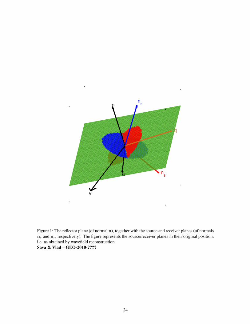
By construction, vectors n, ns, nr and q are co-planar and vectors n and q are orthogonal, Figure 1.151

With these definitions, the (planar) source and receiver wavefields are given by the expressions:152

ns · x = 0 , (6)

nr · x = 0 . (7)

Here, x represents space coordinates and, without loss of generality, we assume that the origin of153

the time axis is set when the source and receiver planes intersect at the reflection point. Equations 6154

and 7 define the conventional imaging condition given by equations 1 and 2. This condition states155

that an image is formed when the source and receiver wavefields are time-coincident at reflection156

points. In Equations 6 and 7, we explicitly impose the condition that the source and receiver planes157

and the reflector plane intersect at the image point.158

Similarly, we can rewrite the extended imaging condition using the planar approximation of the159

source and receiver wavefields using the expressions:160

ns · (x− λ) = −vτ , (8)

nr · (x + λ) = +vτ . (9)

As discussed earlier, λ and τ are space- and time-lags, and v represents the local velocity at the161

image point, assumed to be constant in the immediate vicinity of this point. This assumption is162

8

justified by the need to operate with planar objects, as indicated earlier. With this construction, the163

source and receiver planes are shifted relative to one-another by equal quantities in the positive and164

negative directions and in space and time, equations 3-4.165

We can eliminate the space variable x by substituting equation 6 in equation 8 and equation 7166

in equation 9:167

ns · λ = vτ , (10)

nr · λ = vτ . (11)

Furthermore, we can re-arrange the system given by equations 10 and 11 by sum and difference of168

the equations:169

(ns + nr) · λ = 2vτ , (12)

(ns − nr) · λ = 0 . (13)

So far, we have not assumed any relation between the vectors characterizing the source and170

receiver planes, ns and nr. However, if the source and receiver wavefields correspond to a reflection171

from a planar interface, these vectors are not independent of one-another, but are related by Snell’s172

law which can be formulated as173

nr = ns − 2 (ns · n)n . (14)

This relations follows from geometrical considerations and it is based on the conservation of ray174

vector projection along the reflector. Equation 14 is only valid for PP reflections in an isotropic175

medium.176

9

Substituting Snell’s law into the system 12-13, and after trivial manipulations of the equations,177

we obtain the system:178

[ns − (ns · n)n] · λ = vτ , (15)

(ns · n) (n · λ) = 0 . (16)

In general, the plane characterizing the source wavefield is not orthogonal to the reflection plane179

(there would be no reflection in that case), therefore we can simplify equation 16 by dropping the180

term (ns · n) 6= 0. Moreover, we can replace in equation 15 the expression in the square bracket181

with the quantity q sin θ, where q is the unit vector characterizing the line at the intersection of the182

reflection and reflector planes, and θ is the reflection angle contained in the reflection plane. With183

these simplifications, the system 15-16 can be re-written as:184

(q · λ) sin θ = vτ , (17)

n · λ = 0 . (18)

The system 17-18 allows for a straightforward physical interpretation of the extended imaging con-185

dition. First, the expression 18 indicates that of all possible space-lags that can be applied to the186

reconstructed wavefields, the only ones that contribute to the extended image are those for which187

the space-lag vector λ is orthogonal to the reflector normal vector n. Furthermore, assuming that188

the space-shift applied to the source and receiver planes is contained in the reflector plane, i.e.189

λ ⊥ n, then the expression 17 describe the moveout function in an extended gather as a function190

of the space-lag λ, the time lag τ , the reflection angle θ, the orientation vector q. The vector q is191

orthogonal to the reflector normal and depends on the reflection azimuth angle φ.192

10

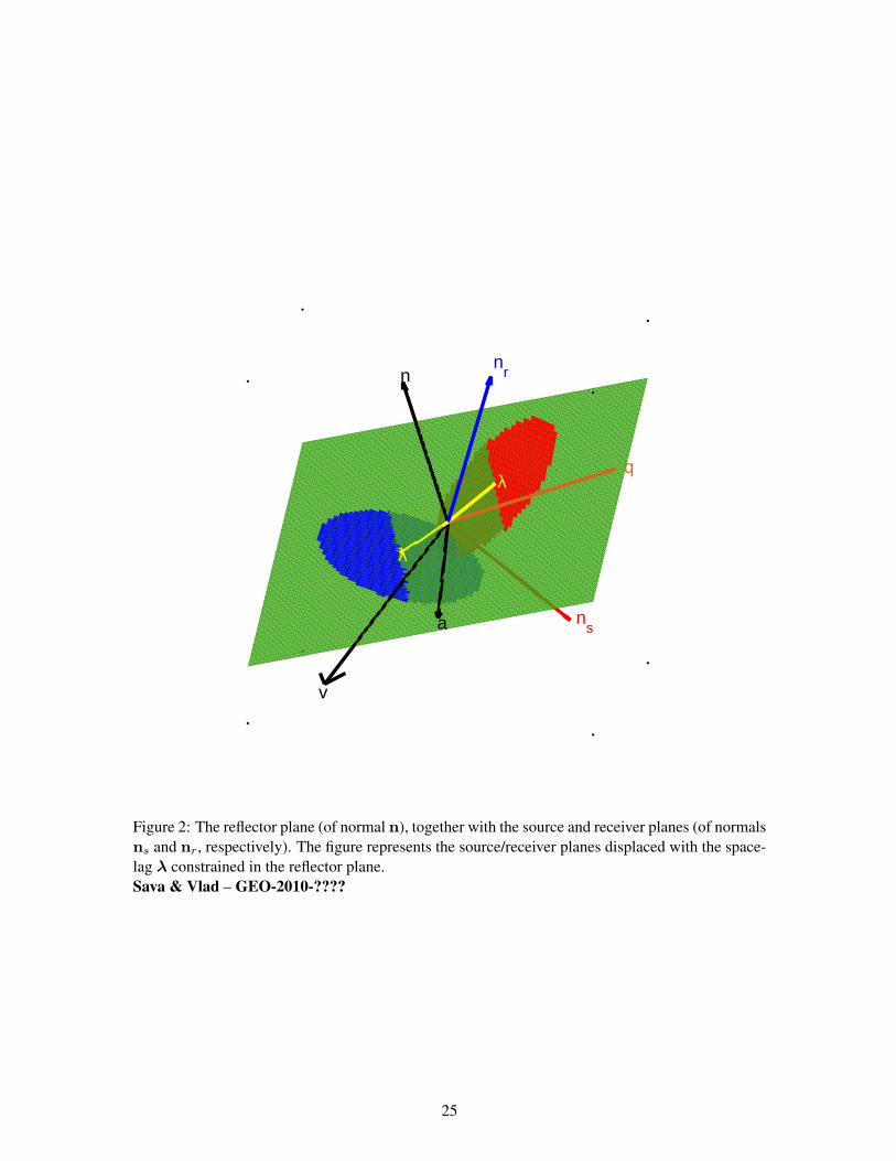
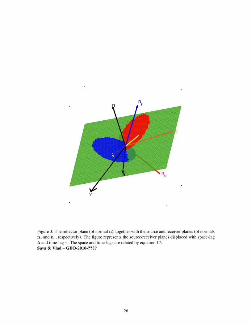
Figures 1-3 illustrate the process involved in the extended imaging condition and describe193

pictorially its physical meaning. Figure 1 shows the source and receiver planes, as well as the194

reflector plane together with their unit vector normals. Figure 2 shows the source and receiver195

planes displaced by the space lag vector λ contained in the reflector plane, as indicated by equa-196

tion 18. The displaced planes do not intersect at the reflection plane, thus they do not contribute197

to the extended image at this point. However, with the application of time shits with the quantity198

τ = (q · λ) sin θ/v, i.e. a translation in the direction of plane normals, the source and receiver199

planes are restored to the image point, thus contributing to the extended image, Figure 3.200

ANGLE DECOMPOSITION

In this section we discuss the steps required to transform lag-domain CIPs into angle-domain CIPs201

using the moveout function derived in the preceding section. We also present the algorithm used for202

angle decomposition and illustrate it using a simple 3D model of a horizontal reflector in a medium203

with constant velocity which allows us to validate analytically the procedure.204

The outer loop of the algorithm is over the CIPs evaluated during migration. The angle decom-205

position of individual CIPs is independent of one-another, therefore the algorithm is easily paral-206

lelizable over the outer loop. At every CIP, we need to access the information about the reflector207

normal (n) and about the local velocity (v). The reflector dip information can be extracted from the208

conventional image, and the velocity is the same as the one used for migration.209

Prior to the angle decomposition, we also need to define a direction relative to which we mea-210

sure the reflection azimuth. This direction is arbitrary and depends on the application of the angle211

decomposition. Typically, the azimuth is defined relative to a reference direction (e.g. North). Here,212

we define this azimuth direction using an arbitrary vector v. Using the reflector normal (n) we can213

11

build the projection of the azimuth vector (a) in the reflector plane as214

a = (n× v)× n . (19)

This construction assures that vector a is contained in the reflector plane (i.e. it is orthogonal on n)215

and that it is co-planar with vectors n and v, Figure 1. Of course, this construction is just one of the216

many possible definitions of the azimuth reference. In the following, we measure the azimuth angle217

φ relative to vector a and the reflection angle θ relative to the normal to the reflector given by vector218

n.219

Then, for every azimuth angle φ, using the reflector normal (n) and the azimuth reference (a),220

we can construct the trial vector q which lies at the intersection of the reflector and the reflection221

planes. We scan over all possible vectors q, although only one azimuth corresponds to the reflection222

from a given shot. This scan ensures that we capture the reflection information from all shots in223

the survey. Given the reflector normal (the axis of rotation) and the trial azimuth angle φ, we can224

construct the different vectors q by the application of the rotation matrix225

Q (n, φ) =

n2x +

(n2y + n2

z

)cosφ nxny (1− cosφ)− nz sinφ nxnz (1− cosφ) + ny sinφ

nynx (1− cosφ) + nz sinφ n2y +

(n2z + n2

x

)cosφ nynz (1− cosφ)− nx sinφ

nznx (1− cosφ)− ny sinφ nzny (1− cosφ) + nx sinφ n2z +

(n2x + n2

y

)cosφ

(20)

to the azimuth reference vector a, i.e.226

q = Q (n, φ)a . (21)

In this formulation, the normal vector n of components {nx, ny, nz} can take arbitrary orientations227

12

and does not need to be normalized. Then, for every reflection angle θ, we map the lag-domain228

CIP to the angle-domain by summation over the surface defined by equation 17. This operation229

represents a planar Radon transform (a slant-stack) over an analytically-defined surface in the {λ, τ}230

space. The output is the representation of the CIP in the angle-domain. In order to preserve the231

signal bandwidth, the slant-stack needs to use a “rho filter” which compensates the high frequency232

decay caused by the summation (Claerbout, 1976). The explicit algorithm for angle decomposition233

is given in Appendix A.234

Consider a simple 3D model consisting of a horizontal reflector in a constant velocity medium.235

We simulate one shot in the center of the model at coordinates x = 4 km and y = 4 km, with236

receivers distributed uniformly on the surface on a grid spaced at every 20 m in the x and y direc-237

tions. We use time-domain finite-differences for modeling. Figure 4 represents the image obtained238

by wave-equation migration of the simulated shot using downward continuation. The illumination239

is limited to a narrow region around the shot due to the limited array aperture.240

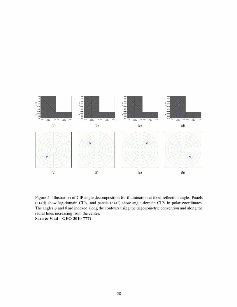
Figures 5(a)-5(d) depict CIPs obtained by migration of the simulated shot at the reflector depth241

and at coordinates {x, y} equal to {3.2, 3.2} km, {3.2, 4.8} km, {4.8, 4.8} km and {4.8, 3.2} km,242

respectively. For these CIPs, the reflection angle is invariant θ = 48.5◦, but the azimuth angles243

relative to the x axis are −135◦, +135◦, +45◦ and −45◦, respectively. Figures 5(e)-5(h) show the244

angle decomposition in polar coordinates. Here, we use the trigonometric convention to represent245

the azimuth angle φ and we represent the reflection angle in every azimuth in the radial direction246

(with normal incidence at the center of the plot). Each radial line corresponds to 30◦ and each247

circular contour corresponds to 15◦.248

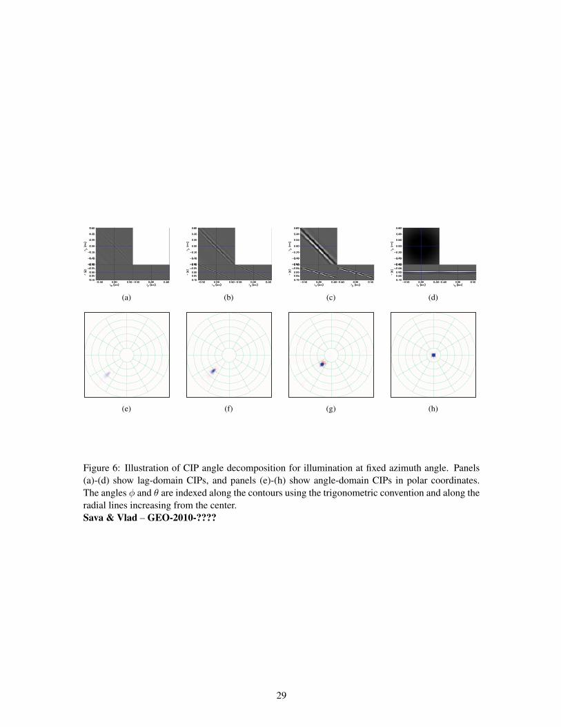
Similarly, Figures 6(a)-6(d) depict CIPs obtained by migration of the simulated shot the re-249

flector depth and at coordinates {x, y} equal to {2.8, 2.8} km, {3.2, 3.2} km, {3.6, 3.6} km and250

13

{4.0, 4.0} km, respectively. For these CIPs, the azimuth angle is invariant φ = −135◦, but the251

reflection angles relative to the reflector normal are 59.5◦, 48.5◦, 29.5◦, and 0◦ respectively.252

In all examples, the decomposition angles correspond to the theoretical values, thus confirming253

the validity of our decomposition.254

EXAMPLES

We illustrate the method discussed in the preceding section with common-image-point-gathers con-255

structed using the wide-azimuth SEAM data (). Figure 7 shows the velocity model in the area used256

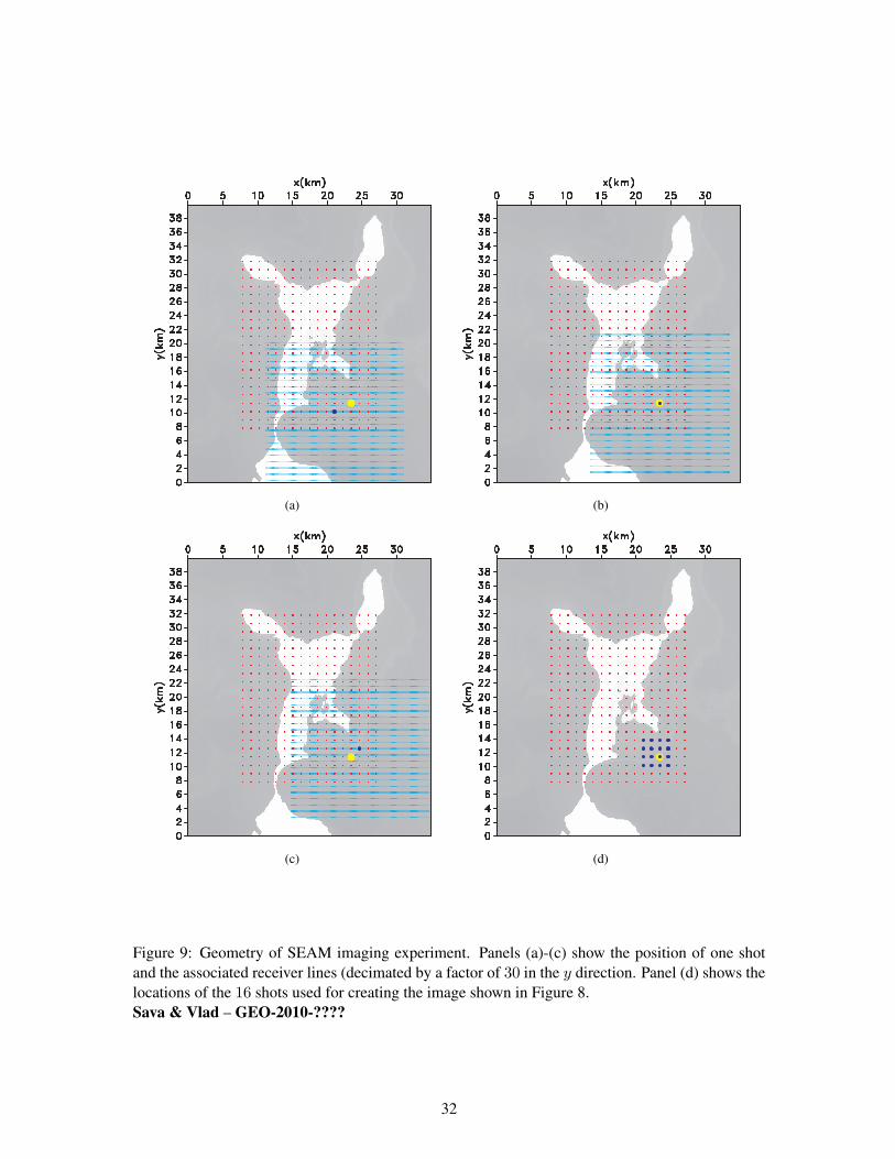
for imaging. For demonstration, we consider 16 shots located at the locations of the thick dots in257

Figure 9(d). The thin dots represent all the 357 shots available in one of the SEAM data subsets.258

The solid lines in Figures 9(a)-9(b) depict the decimated receiver lines for each of the 3 shots shown.259

In all panels 9(a)-9(d), the large dot indicates the surface projection of the CIP used for illustration,260

located at coordinates {x, y, z} = {23.450, 11.425, 2.38} km. For this example we consider the261

azimuth reference vector oriented in the x direction, i.e. v = {1, 0, 0}.262

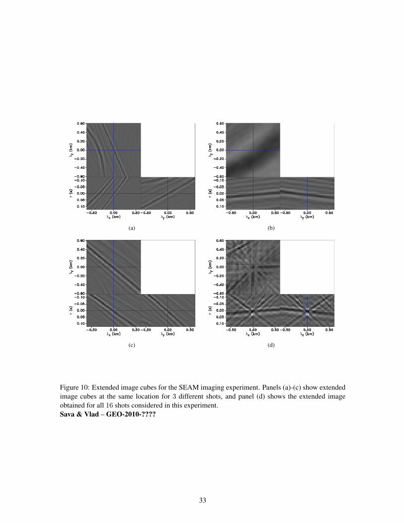
Figures 10(a)-10(c) show the extended image obtained at the CIP location indicated earlier using263

migration by downward continuation. The extended image cubes use 41 grid points in the hx and264

hy directions sampled on the image grid, i.e. at every 30 m, and 31 grid points in the τ direction265

sampled on the data grid, i.e. at every 8 ms. The vertical lag hz is not computed in this example,266

since the analyzed reflector is nearly-horizontal. This lag is computed in the decomposition process267

from the horizontal lag and from the known information about the normal to the reflector at the268

given position. Figure 10(d) shows the extended image obtained for all 16 shots used for imaging.269

Although here we show the extended image cubes for independent shots, in practice these cubes270

need not be computed separately – the decomposition separates the information corresponds to271

14

different angles of incidence, as shown in this simple example.272

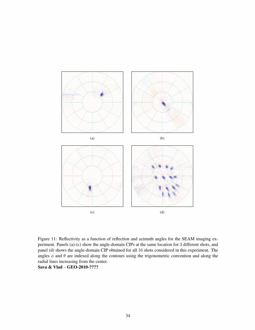
Finally, Figures 11(a)-11(d) show the angle-domain decomposition of the extended image cubes273

shown in Figures 10(a)-10(d), respectively. In these plots, the circles indicating the reflection angles274

are drawn at every 5◦ and the radial lines indicating the azimuth directions are drawn at every 15◦.275

Given the sparse shot sampling, the CIP is sparsely illuminated, but at the correct reflection and276

azimuth angles.277

DISCUSSION

As indicated in the preceding sections, we do not need to compute all space-lags at the considered278

CIP positions. We could compute just two of them, e.g. λx and λy as shown in the examples of279

this paper, and then reconstruct the third lag using the information given by the reflector normal at280

the CIP position. If the reflector is nearly vertical, it may be more relevant to compute the vertical281

and one horizontal space-lags. Alternatively, we could avoid computing the reflector normal vector282

from the conventional image, but instead compute all three components of the space-lag vector λ.283

In this case, as indicated by Sava and Vasconcelos (2010), we could estimate the reflector dip from284

the lag information prior to the angle decomposition.285

We have also noted earlier in the paper that the relevant space-lags are constructed in the re-286

flector plane. This fact is a direct consequence of the fact that we have considered equal but with287

opposite sign time-shift of the source and receiver wavefields. Without this convention, the angle288

decomposition problem becomes more complex. In our experience to date, we did not find the need289

to relax this requirement.290

The angle-domain CIPs accurately indicate the sampling of the reflector as a function of azimuth291

and reflection angles. If the shot distribution is sparse, or if the sub-surface geology creates shadow292

15

zones, the illumination is also sparse. This is both beneficial, assuming that the angle-domain CIPs293

are used to evaluate illumination, but it can also be a drawback if the angle-domain CIPs are used for294

AVA or MVA. However, a sparse sampling of a reflector is not a feature of the angle decomposition,295

but a feature of the acquisition geometry. Neither our, nor any other angle decomposition, can296

compensate for the lack of adequate data illuminating the subsurface on a dense angular grid.297

Finally, we note that the most likely applications for angle decomposition in complex geology298

is the study of the reflector illumination itself. Assuming that the sampling is sufficiently dense and299

that the imaging velocity is accurately known, then we can use the angle decomposition discussed in300

this paper to evaluate amplitude variation with azimuth and reflection angles. However, we empha-301

size that this is a relevant exercise only if the reflector illumination is sufficiently dense. Otherwise,302

AVA effects overlap with illumination effects, rendering the analysis unreliable. Migration velocity303

analysis in the angle domain may also suffer from the lack of adequate illumination. This partial304

illumination may deteriorate the moveout which would otherwise be observed in the extended im-305

age domain. Furthermore, we do not advocate an implementation of MVA in the angle-domain,306

but rather in the extended image domain which contains all the relevant information and avoids the307

additional step of angle decomposition. An extensive discussion of this problem is outside the scope308

of our paper.309

CONCLUSIONS

Angle decomposition based on wavefield extrapolation methods is characterized by robustness in310

areas with sharp velocity variation and by accuracy in the presence of steeply dipping reflectors.311

Extended common-image-point gathers constructed at discrete image points provide sufficient in-312

formation for angle decomposition. The decomposition is based on the planar approximation of313

16

the source and receiver wavefields in the immediate vicinity of the image points. Both space-lag314

and the time-lag extensions are required to completely characterize the reflection geometry given315

by the local reflection and azimuth angles. However, assuming that information about the reflector316

slope is available, we could avoid computing one lag of the extended image, usually the vertical.317

This increases the computational efficiency of the method and makes it affordable for large-scale318

wide-azimuth imaging projects.319

ACKNOWLEDGMENTS

Paul Sava acknowledges the support of the sponsors of the Center for Wave Phenomena at Colorado320

School of Mines. Ioan Vlad acknowledges Statoil for support of this research. The reproducible321

numeric examples in this paper use the Madagascar open-source software package freely avail-322

able from http://www.reproducibility.org. The 3D data used in this paper are owned by the SEG323

Advanced Modeling Corporation and were provided to CWP by ExxonMobil Upstream Research324

Company.325

17

REFERENCES

Berkhout, A. J., 1982, Imaging of acoustic energy by wave field extrapolation: Elsevier.326

Biondi, B., and P. Sava, 1999, Wave-equation migration velocity analysis: 69th Annual International327

Meeting, SEG, Expanded Abstracts, 1723–1726.328

Biondi, B., and W. Symes, 2004, Angle-domain common-image gathers for migration velocity329

analysis by wavefield-continuation imaging: Geophysics, 69, 1283–1298.330

Brandsberg-Dahl, S., M. V. de Hoop, and B. Ursin, 2003, Focusing in dip and AvA compensation331

on scattering-angle/azimuth common image gathers: Geophysics, 68, 232–254.332

Claerbout, J. F., 1976, Fundamentals of geophysical data processing: Blackwell Scientific Publica-333

tions.334

——–, 1985, Imaging the Earth’s interior: Blackwell Scientific Publications.335

Clarke, R., G. Xia, N. Kabir, L. Sirgue, and S. Michell, 2006, Case study: A large 3D wide azimuth336

ocean bottom node survey in deepwater gom: SEG Technical Program Expanded Abstracts, 25,337

1128–1132.338

Clayton, R. W., and R. H. Stolt, 1981, A Born-WKBJ inversion method for acoustic reflection data:339

Geophysics, 46, 1559–1567.340

de Bruin, C. G. M., C. P. A. Wapenaar, and A. J. Berkhout, 1990, Angle-dependent reflectivity by341

means of prestack migration: Geophysics, 55, 1223–1234.342

Faye, J. P., and J. P. Jeannot, 1986, Prestack migration velocities from focusing depth analysis: 56th343

Ann. Internat. Mtg., Soc. of Expl. Geophys., Session:S7.6.344

Gray, S. H., J. Etgen, J. Dellinger, and D. Whitmore, 2001, Seismic migration problems and solu-345

tions: Geophysics, 66, 1622–1640.346

Koren, Z., I. Ravve, E. Ragoza, A. Bartana, P. Geophysical, and D. Kosloff, 2008, Full-azimuth347

angle domain imaging: SEG Technical Program Expanded Abstracts, 27, 2221–2225.348

18

MacKay, S., and R. Abma, 1992, Imaging and velocity estimation with depth-focusing analysis:349

Geophysics, 57, 1608–1622.350

——–, 1993, Depth-focusing analysis using a wavefront-curvature criterion: Geophysics, 58, 1148–351

1156.352

Michell, S., E. Shoshitaishvili, D. Chergotis, J. Sharp, and J. Etgen, 2006, Wide azimuth streamer353

imaging of mad dog; have we solved the subsalt imaging problem?: SEG Technical Program354

Expanded Abstracts, 25, 2905–2909.355

Mosher, C. C., D. J. Foster, and S. Hassanzadeh, 1997, Common angle imaging with offset plane356

waves: 67th Ann. Internat. Mtg, Soc. of Expl. Geophys., 1379–1382.357

Nemeth, T., 1995, Velocity estimation using tomographic depth-focusing analysis: 65th Ann. Inter-358

nat. Mtg, Soc. of Expl. Geophys., 465–468.359

——–, 1996, Relating depth-focusing analysis to migration velocity analysis: 66th Ann. Internat.360

Mtg, Soc. of Expl. Geophys., 463–466.361

Prucha, M., B. Biondi, and W. Symes, 1999, Angle-domain common image gathers by wave-362

equation migration: 69th Ann. Internat. Mtg, Soc. of Expl. Geophys., 824–827.363

Regone, C., 2006, Using 3D finite-difference modeling to design wide azimuth surveys for improved364

subsalt imaging: SEG Technical Program Expanded Abstracts, 25, 2896–2900.365

Rickett, J., and P. Sava, 2002, Offset and angle-domain common image-point gathers for shot-profile366

migration: Geophysics, 67, 883–889.367

Sava, P., and B. Biondi, 2004a, Wave-equation migration velocity analysis - I: Theory: Geophysical368

Prospecting, 52, 593–606.369

——–, 2004b, Wave-equation migration velocity analysis - II: Subsalt imaging examples: Geophys-370

ical Prospecting, 52, 607–623.371

Sava, P., and S. Fomel, 2003, Angle-domain common image gathers by wavefield continuation372

19

methods: Geophysics, 68, 1065–1074.373

——–, 2005, Coordinate-independent angle-gathers for wave equation migration: 75th Annual In-374

ternational Meeting, SEG, Expanded Abstracts, 2052–2055.375

——–, 2006, Time-shift imaging condition in seismic migration: Geophysics, 71, S209–S217.376

Sava, P., and I. Vasconcelos, 2010, Extended imaging condition for wave-equation migration: Geo-377

physical Prospecting, in press.378

Shen, P., W. Symes, and C. C. Stolk, 2003, Differential semblance velocity analysis by wave-379

equation migration: 73rd Ann. Internat. Mtg., Soc. of Expl. Geophys., 2132–2135.380

Shen, P., and W. W. Symes, 2008, Automatic velocity analysis via shot profile migration: Geo-381

physics, 73, VE49–VE59.382

Stolk, C. C., and W. W. Symes, 2004, Kinematic artifacts in prestack depth migration: Geophysics,383

69, 562–575.384

Stolt, R. H., and A. B. Weglein, 1985, Migration and inversion of seismic data: Geophysics, 50,385

2458–2472.386

Symes, W., 2009, Migration velocity analysis and waveform inversion: Geophysical Prospecting,387

56, 765–790.388

Weglein, A. B., and R. H. Stolt, 1999, Migration-inversion revisited (1999): The Leading Edge, 18,389

950–952.390

Wu, R.-S., and L. Chen, 2006, Directional illumination analysis using beamlet decomposition and391

propagation: Geophysics, 71, S147–S159.392

Xie, X., and R. Wu, 2002, Extracting angle domain information from migrated wavefield: 72nd393

Ann. Internat. Mtg, Soc. of Expl. Geophys., 1360–1363.394

Xu, S., H. Chauris, G. Lambare, and M. S. Noble, 1998, Common angle image gather: A new395

strategy for imaging complex media: 68th Ann. Internat. Mtg, Soc. of Expl. Geophys., 1538–396

20

1541.397

Zhu, X., and R.-S. Wu, 2010, Imaging diffraction points using the local image matrices generated398

in prestack migration: Geophysics, 75, S1–S9.399

APPENDIX A

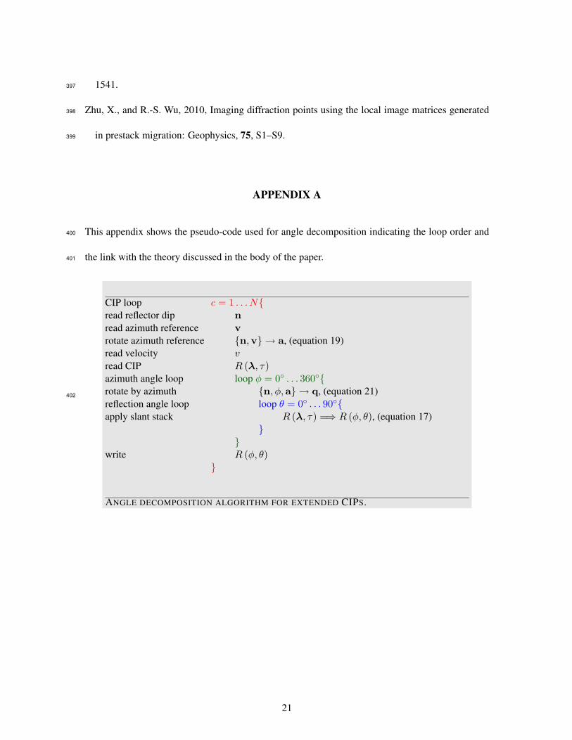
This appendix shows the pseudo-code used for angle decomposition indicating the loop order and400

the link with the theory discussed in the body of the paper.401

CIP loop c = 1 . . . N{read reflector dip nread azimuth reference vrotate azimuth reference {n,v} → a, (equation 19)read velocity vread CIP R (λ, τ)azimuth angle loop loop φ = 0◦ . . . 360◦{rotate by azimuth {n, φ,a} → q, (equation 21)reflection angle loop loop θ = 0◦ . . . 90◦{apply slant stack R (λ, τ) =⇒ R (φ, θ), (equation 17)

}}

write R (φ, θ)}

ANGLE DECOMPOSITION ALGORITHM FOR EXTENDED CIPS.

402

21

LIST OF FIGURES

1 The reflector plane (of normal n), together with the source and receiver planes (of normals403

ns and nr, respectively). The figure represents the source/receiver planes in their original position,404

i.e. as obtained by wavefield reconstruction.405

2 The reflector plane (of normal n), together with the source and receiver planes (of normals406

ns and nr, respectively). The figure represents the source/receiver planes displaced with the space-407

lag λ constrained in the reflector plane.408

3 The reflector plane (of normal n), together with the source and receiver planes (of normals409

ns and nr, respectively). The figure represents the source/receiver planes displaced with space-lag410

λ and time-lag τ . The space and time-lags are related by equation 17.411

4 The image obtained for a horizontal reflector in constant velocity using one shot located412

in the center of the model.413

5 Illustration of CIP angle decomposition for illumination at fixed reflection angle. Panels414

(a)-(d) show lag-domain CIPs, and panels (e)-(f) show angle-domain CIPs in polar coordinates. The415

angles φ and θ are indexed along the contours using the trigonometric convention and along the ra-416

dial lines increasing from the center.417

6 Illustration of CIP angle decomposition for illumination at fixed azimuth angle. Panels418

(a)-(d) show lag-domain CIPs, and panels (e)-(h) show angle-domain CIPs in polar coordinates.419

The angles φ and θ are indexed along the contours using the trigonometric convention and along the420

radial lines increasing from the center.421

7 A subset of the SEAM velocity model used for the imaging example in Figures 8-11(d).422

8 Conventional image obtained using wavefield extrapolation with the 16 shots shown in423

Figure 9(d).424

9 Geometry of SEAM imaging experiment. Panels (a)-(c) show the position of one shot and425

22

the associated receiver lines (decimated by a factor of 30 in the y direction. Panel (d) shows the426

locations of the 16 shots used for creating the image shown in Figure 8.427

10 Extended image cubes for the SEAM imaging experiment. Panels (a)-(c) show extended428

image cubes at the same location for 3 different shots, and panel (d) shows the extended image429

obtained for all 16 shots considered in this experiment.430

11 Reflectivity as a function of reflection and azimuth angles for the SEAM imaging exper-431

iment. Panels (a)-(c) show the angle-domain CIPs at the same location for 3 different shots, and432

panel (d) shows the angle-domain CIP obtained for all 16 shots considered in this experiment. The433

angles φ and θ are indexed along the contours using the trigonometric convention and along the434

radial lines increasing from the center.435

436

23

q

ns

nr

a

n

v

Figure 1: The reflector plane (of normal n), together with the source and receiver planes (of normalsns and nr, respectively). The figure represents the source/receiver planes in their original position,i.e. as obtained by wavefield reconstruction.Sava & Vlad – GEO-2010-????

24

q

ns

λ

nr

a

n

λ

v

Figure 2: The reflector plane (of normal n), together with the source and receiver planes (of normalsns and nr, respectively). The figure represents the source/receiver planes displaced with the space-lag λ constrained in the reflector plane.Sava & Vlad – GEO-2010-????

25

qλ

ns

nr

a

n

λ

v

Figure 3: The reflector plane (of normal n), together with the source and receiver planes (of normalsns and nr, respectively). The figure represents the source/receiver planes displaced with space-lagλ and time-lag τ . The space and time-lags are related by equation 17.Sava & Vlad – GEO-2010-????

26

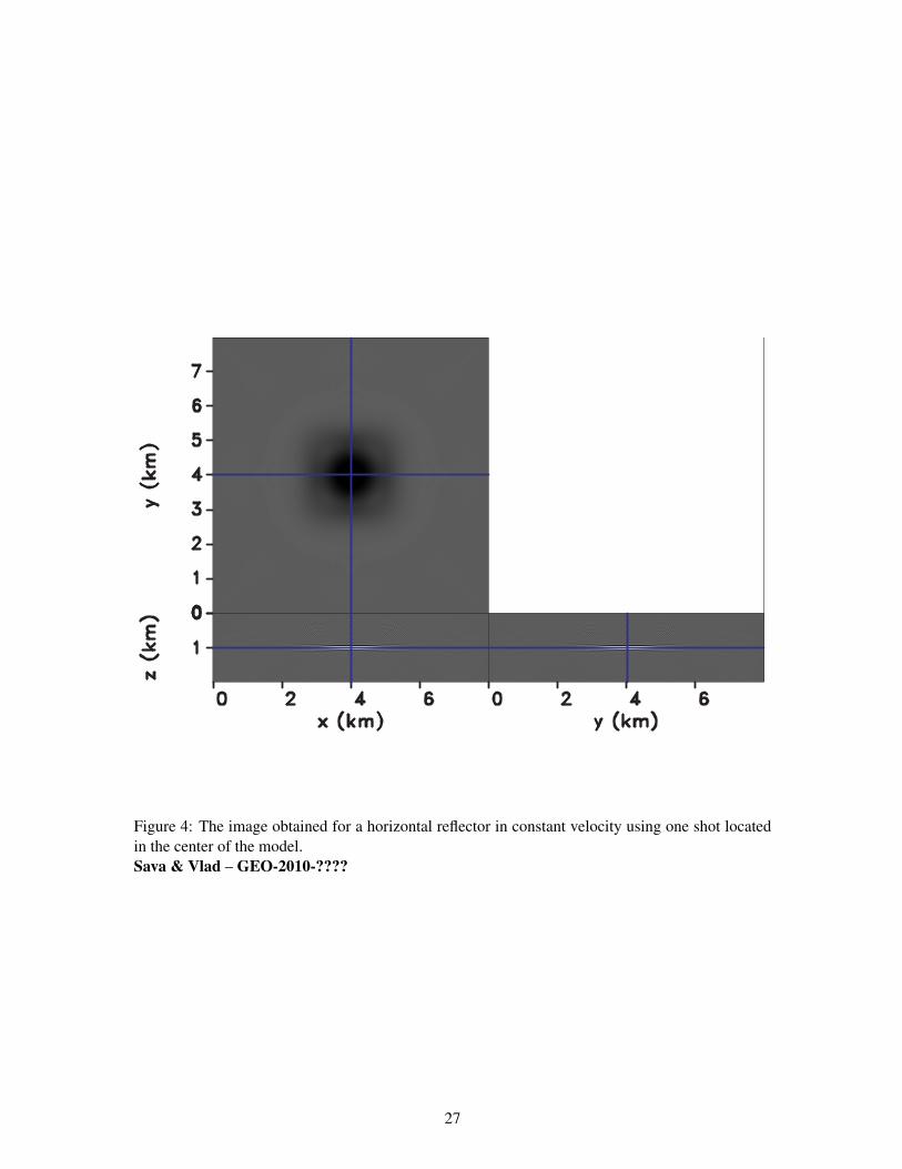
Figure 4: The image obtained for a horizontal reflector in constant velocity using one shot locatedin the center of the model.Sava & Vlad – GEO-2010-????

27

(a) (b) (c) (d)

(e) (f) (g) (h)

Figure 5: Illustration of CIP angle decomposition for illumination at fixed reflection angle. Panels(a)-(d) show lag-domain CIPs, and panels (e)-(f) show angle-domain CIPs in polar coordinates.The angles φ and θ are indexed along the contours using the trigonometric convention and along theradial lines increasing from the center.Sava & Vlad – GEO-2010-????

28

(a) (b) (c) (d)

(e) (f) (g) (h)

Figure 6: Illustration of CIP angle decomposition for illumination at fixed azimuth angle. Panels(a)-(d) show lag-domain CIPs, and panels (e)-(h) show angle-domain CIPs in polar coordinates.The angles φ and θ are indexed along the contours using the trigonometric convention and along theradial lines increasing from the center.Sava & Vlad – GEO-2010-????

29

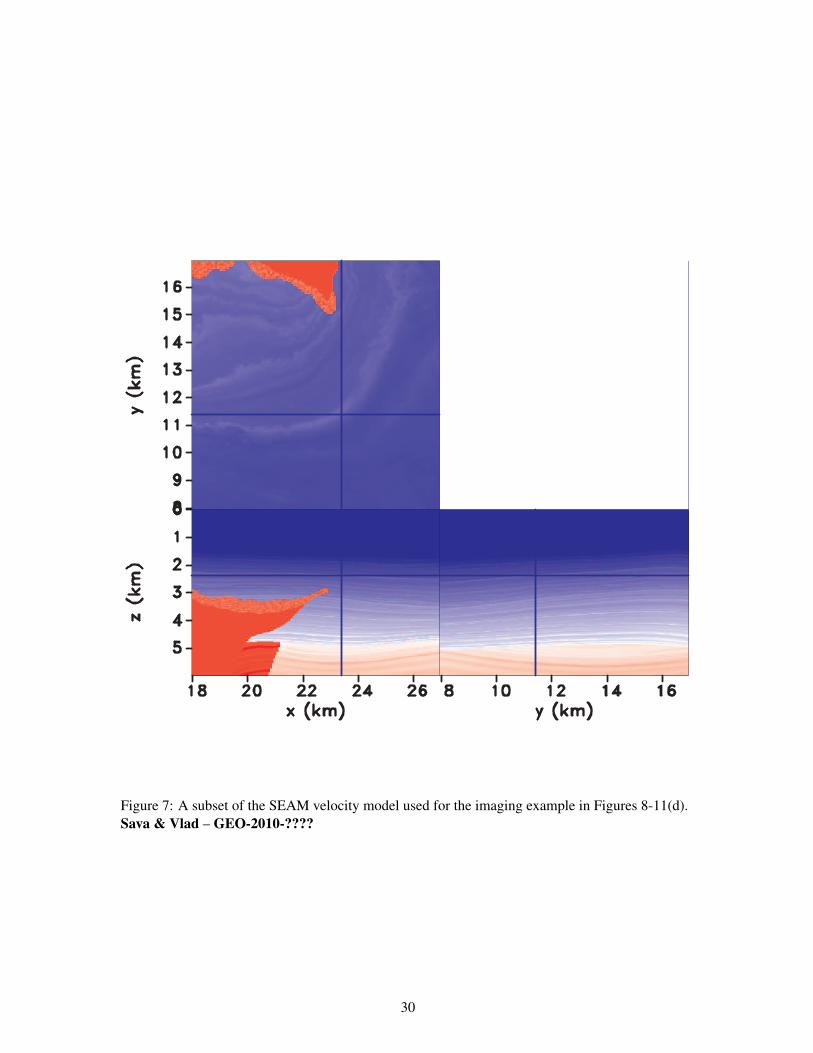
Figure 7: A subset of the SEAM velocity model used for the imaging example in Figures 8-11(d).Sava & Vlad – GEO-2010-????

30

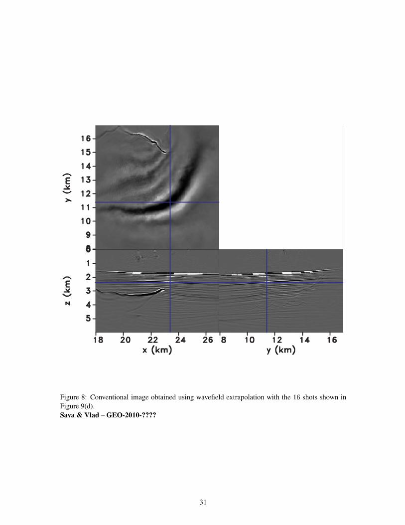
Figure 8: Conventional image obtained using wavefield extrapolation with the 16 shots shown inFigure 9(d).Sava & Vlad – GEO-2010-????

31

(a) (b)

(c) (d)

Figure 9: Geometry of SEAM imaging experiment. Panels (a)-(c) show the position of one shotand the associated receiver lines (decimated by a factor of 30 in the y direction. Panel (d) shows thelocations of the 16 shots used for creating the image shown in Figure 8.Sava & Vlad – GEO-2010-????

32

(a) (b)

(c) (d)

Figure 10: Extended image cubes for the SEAM imaging experiment. Panels (a)-(c) show extendedimage cubes at the same location for 3 different shots, and panel (d) shows the extended imageobtained for all 16 shots considered in this experiment.Sava & Vlad – GEO-2010-????

33

(a) (b)

(c) (d)

Figure 11: Reflectivity as a function of reflection and azimuth angles for the SEAM imaging ex-periment. Panels (a)-(c) show the angle-domain CIPs at the same location for 3 different shots, andpanel (d) shows the angle-domain CIP obtained for all 16 shots considered in this experiment. Theangles φ and θ are indexed along the contours using the trigonometric convention and along theradial lines increasing from the center.Sava & Vlad – GEO-2010-????

34