wide-angle seismic velocities in heterogeneous crust - geophysical

Geophys. J . Int. (1997) 129, 269-280

Wide-angle seismic velocities in heterogeneous crust

John Brittan and Mike Warner Department of Geology, Imperial College, London SW7 2BP, UK. E-mail: [email protected]. uk

Accepted 1996 December 10. Received 1996 December 5; in original form 1996 September 6

SUMMARY Seismic velocities measured by wide-angle surveys are commonly used to constrain material composition in the deep crust. Therefore, it is important to understand how these velocities are affected by the presence of multiscale heterogeneities. The effects may be characterised by the scale of the heterogeneity relative to the dominant seismic wavelength (A); what is clear is that heterogeneities of all scales and strengths bias wide- angle velocities to some degree. Waveform modelling was used to investigate the apparent wide-angle P-wave velocities of different heterogeneous lower crusts. A constant composition (50 per cent felsic and 50 per cent ultramafic) was formed into a variety of 1- and 2-D heterogeneous arrangements and the resulting wide-angle seismic velocity was estimated. Elastic, 1-D models produced the largest velocity shift relative to the true average velocity of the medium (which is the velocity of an isotropic mixture of the two components). Thick (width>>A) horizontal layers, as a result of Fermat’s Principle, provided the largest increase in velocity; thin (width << 2) vertical layers produced the largest decrease in velocity. Acoustic 2-D algorithms were shown to be inadequate for modelling the kinematics of waves in bodies with multiscale heterogeneities. Elastic, 2-D modelling found velocity shifts (both positive and negative) that were of a smaller magnitude than those produced by 1-D models. The key to the magnitude of the velocity shift appears to be the connectivity of the fast (and/or slow) components. Thus, the models with the highest apparent levels of connectivity between the fast phases, the 1-D layers, produced the highest-magnitude velocity shifts. To understand the relationship between measured seismic velocities and petrology in the deep crust it is clear that high-resolution structural information (which describes such connectivity) must be included in any modelling.

Key words: crust, inhomogeneous media, seismic velocities

INTRODUCTION

The interior of the Earth is clearly not a simple assemblage of concentric shells whose compositions and organisations are homogeneous. Surface exposures of crustal material suggest that the interior of the Earth is a heterogeneous composite, the general definition of heterogeneity being a spatial variation of a particular physical characteristic (Macbeth 1995). The scale length of the heterogeneities present in the Earth’s crust range from the megascale (tectonic features such as plates or orogenic belts of hundreds of kilometres extent) down to below the microscale (the minerals that compose these features whose characteristic size is often less than 1 mm).

The information that a seismic wave carries about a medium it has traversed is dependent upon the size, strength and arrangement of the heterogeneities of which the medium is composed. If the surface observer is to interpret this information correctly, it is vital to understand the effects of

heterogeneity. In particular, it is important to discover whether certain types of heterogeneity can unduly dominate the response to the seismic waves and thus mislead an interpreter who has no apriori knowledge of the actual structure. This is particularly important in the case of the exploration of the continental and marginal lower crust for two reasons. First, the information provided by seismic experiments over these areas is the highest-resolution in situ information available, and second, the results from such experiments suggest a diverse pattern of heterogeneity, particularly in the lower crust (Sadowiak, Meissner & Brown 1991; Mooney & Meissner 1992). The evidence from reflection profiles clearly indicates that wide-angle seismic waves traverse areas of lower crust that are highly heterogeneous. In this paper we investigate the effect of multiscale heterogeneities upon the traveltimes of waves traversing such regions, and, in particular, we discuss the wide-angle apparent velocities of heterogeneous arrangements of lower-crustal material. The apparent velocity

269 0 1997 RAS

Dow

nloaded from https://academ

ic.oup.com/gji/article/129/2/269/590166 by guest on 27 February 2022

210 J. Brittan and M. Warner

[sometimes known as the effective velocity (Brittan & Warner 1996)] is defined as the gross P-wave seismic velocity the heterogeneous medium would have if it was interpreted to be isotropic and homogeneous. Our approach to this problem is first to give an overview of how different scales of heterogeneity modify the wavefield and then to use modelling to quantify the effects of these modifications on the velocities measured by wide-angle, deep-crustal seismic surveys. Finally, we discuss

’ the implications of the results for studies of the composition of the lower continental crust.

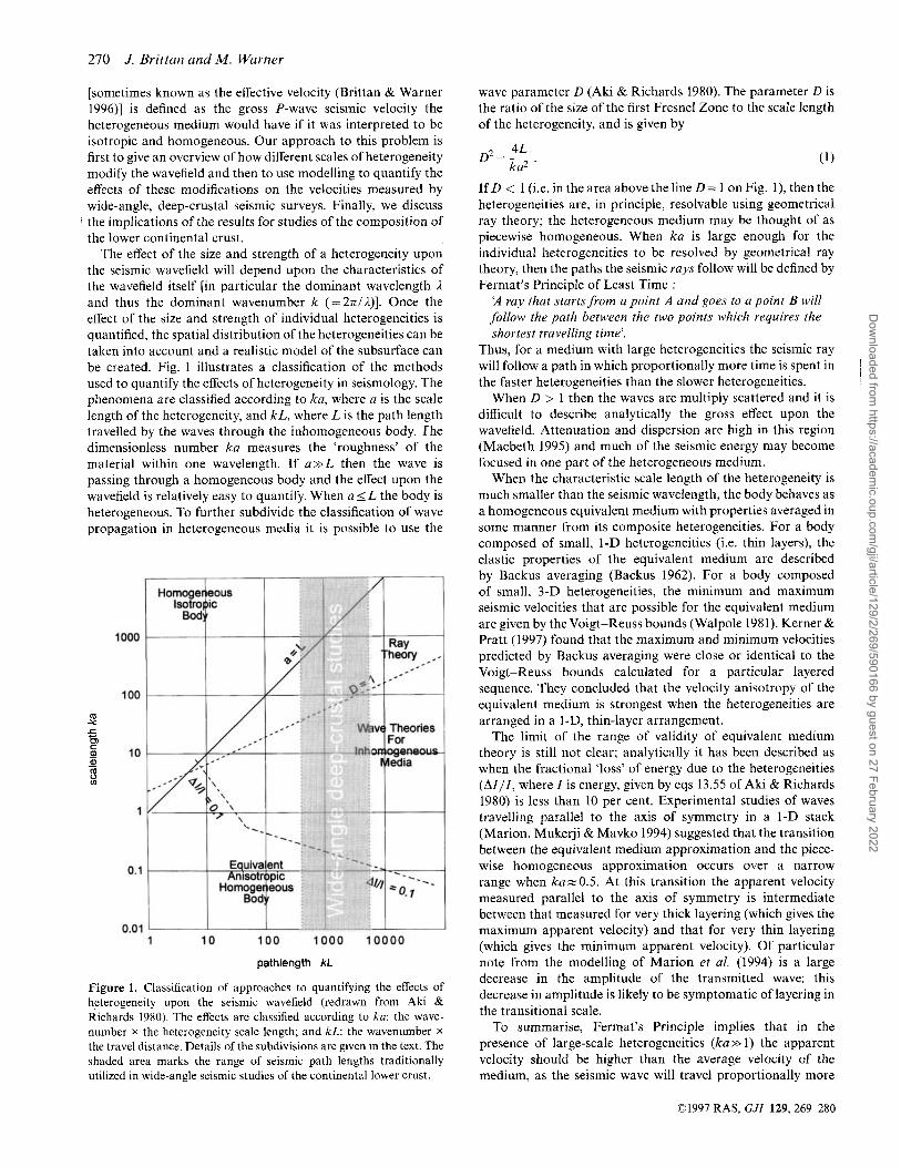
The effect of the size and strength of a heterogeneity upon the seismic wavefield will depend upon the characteristics of the wavefield itself [in particular the dominant wavelength R and thus the dominant wavenumber k (=27t/ l )] . Once the effect of the size and strength of individual heterogeneities is quantified, the spatial distribution of the heterogeneities can be taken into account and a realistic model of the subsurface can be created. Fig. 1 illustrates a classification of the methods used to quantify the effects of heterogeneity in seismology. The phenomena are classified according to ka, where a is the scale length of the heterogeneity, and kL, where L is the path length travelled by the waves through the inhomogeneous body. The dimensionless number ka measures the ‘roughness’ of the material within one wavelength. If a>>L then the wave is passing through a homogeneous body and the effect upon the wavefield is relatively easy to quantify. When a 5 L the body is heterogeneous. To further subdivide the classification of wave propagation in heterogeneous media it is possible to use the

1000

100

10

1

0.1

0.01

pathlength kL

Figure 1. Classification of approaches to quantifying the effects of heterogeneity upon the seismic wavefield (redrawn from Aki & Richards 1980). The effects are classified according to ka: the wavenumber x the heterogeneity scale length; and kL: the wavenumber x the travel distance. Details of the subdivisions are given in the text. The shaded area marks the range of seismic path lengths traditionally utilized in wide-angle seismic studies of the continental lower crust.

wave parameter D (Aki & Richards 1980). The parameter D is the ratio of the size of the first Fresnel Zone to the scale length of the heterogeneity, and is given by

If D < 1 (i.e. in the area above the line D = 1 on Fig. l), then the heterogeneities are, in principle, resolvable using geometrical ray theory; the heterogeneous medium may be thought of as piecewise homogeneous. When ka is large enough for the individual heterogeneities to be resolved by geometrical ray theory, then the paths the seismic rays follow will be defined by Fermat’s Principle of Least Time :

il ray that starts from a point A and goes to a point B will foUow the path between the two points which requires the shortest travelling time’.

Thus, for a medium with large heterogeneities the seismic ray will follow a path in which proportionally more time is spent in the faster heterogeneities than the slower heterogeneities.

When D > 1 then the waves are multiply scattered and it is difficult to describe analytically the gross effect upon the wavefield. Attenuation and dispersion are high in this region (Macbeth 1995) and much of the seismic energy may become focused in one part of the heterogeneous medium.

When the characteristic scale length of the heterogeneity is much smaller than the seismic wavelength, the body behaves as a homogeneous equivalent medium with properties averaged in some manner from its composite heterogeneities. For a body composed of small, I-D heterogeneities (is . thin layers), the elastic properties of the equivalent medium are described by Backus averaging (Backus 1962). For a body composed of small, 3-D heterogeneities, the minimum and maximum seismic velocities that are possible for the equivalent medium are given by theVoigt-Reuss bounds (Walpole 1981). Kerner & Pratt (1997) found that the maximum and minimum velocities predicted by Backus averaging were close or identical to the Voigt-Reuss bounds calculated for a particular layered sequence. They concluded that the velocity anisotropy of the equivalent medium is strongest when the heterogeneities are arranged in a 1-D, thin-layer arrangement.

The limit of the range of validity of equivalent medium theory is still not clear; analytically it has been described as when the fractional ‘loss’ of energy due to the heterogeneities ( A Z / I , where I is energy, given by eqs 13.55 of Aki & Richards 1980) is less than 10 per cent. Experimental studies of waves travelling parallel to the axis of symmetry in a 1-D stack (Marion, Mukerji & Mavko 1994) suggested that the transition between the equivalent medium approximation and the piecewise homogeneous approximation occurs over a narrow range when kaw0.5. At this transition the apparent velocity measured parallel to the axis of symmetry is intermediate between that measured for very thick layering (which gives the maximum apparent velocity) and that for very thin layering (which gives the minimum apparent velocity). Of particular note from the modelling of Marion er al. (1994) is a large decrease in the amplitude of the transmitted wave; this decrease in amplitude is likely to be symptomatic of layering in the transitional scale.

To summarise, Fermat’s Principle implies that in the presence of large-scale heterogeneities (ka >z 1) the apparent velocity should be higher than the average velocity of the medium, as the seismic wave will travel proportionally more

~

01997 RAS, GJI 129,269-280

Dow



Seismic velocities in heterogeneous crust 271

of its path-length within the high-velocity material. At the other end of the scale, small-scale heterogeneities can lead to apparent velocities larger or smaller than the average velocity of the material; the direction of the bias is dependent on the organisation of the heterogeneities relative to the dominant direction of wave propagation. At intermediate scales the effect of the velocity field is suggested to be intermediate between that of the two endmembers (Marion et al. 1994).

MODELLING RESULTS

In this paper we present the results of modelling seismic propagation through simple 1-D and 2-D crusts whose lower halves have highly contrasting structures. The aim of this modelling was to recover the average velocity of the heterogeneous lower crust; this is the velocity that the whole volume of material would have if it was an isotropic mixture of its components. In order to demonstrate clearly the effect of a change in the structure upon the inferred velocity of the lower crust (the apparent velocity), the lower-crustal composition was kept constant. The lower crust was composed of a single material that could be split into two distinct components. Although hampered by sampling bias, which may underestimate the proportion of intermediate rocks in crustal sections [e.g. the exposed lower crust in the Fiordland of New Zealand is extensively metagabbroic diorite (Oliver & Coggon 1979)], laboratory studies of lower-crustal rock samples suggest a bimodal distribution of P-wave velocities between felsic {slow) and mafic/ultramafic (fast) lithologies (Rudnick & Fountain 1995). A clinopyroxene (diopside) was chosen to represent the mafic/ultramafic component and a plagioclase (albite) was chosen to represent the felsic component. The reaon for choosing such a composition was simply to have tRo components with highly contrasting elastic properties, thus representing an extreme case in terms of real crustal composition. In the section on lower continental crust we will discuss in greater detail how the magnitude of heterogeneity-related velocity shifts relates to differences in crustal composition.

The seismic velocities and densities of the two component materials are taken from laboratory studies of single-crystal elastic properties (collated in Brittan & Warner 1996). The velocities have been normalized to standard lower-crustal P-T conditions (0.8 GPa and 400 "C). The albite is modelled to have a P-wave velocity of 6.36 km s-', an S-wave velocity of 3.68 km SKI and a density of 2.62 g cm-3 at lower-crustal conditions; the diopside is modelled to have a P-wave velocity of 7.82 km s-', an S-wave velocity of 4.55 km s-I and a density of 3.28 g cm-3 at lower-crustal conditions.

Lower-crustal velocity is usually determined by using the amplitude and traveltime behaviour of either the strong Moho reflection, PmP, or the lower-crustal diving waves. The lower- crustal diving waves are, on most wide-angle data, of relatively small amplitude and thus of less use than the PmP phase. In all models in this study, there are no velocity gradients within the lower crust and consequently no diving waves. Velocity gradients within the lower crust complicate the interpretation process and may lead to unrealistic levels of lateral heterogeneity. From each of the synthetic seismic responses produced by numerical modelling, the apparent wide-angle velocity was estimated. The arrival times of the PmP phase were picked from the synthetic section and plotted on an x2-t2 graph

(where x is the offset from the source and t is the unreduced picked time). A velocity of the lower crust was then derived using the general form of Dix's equation (Dix 1955).

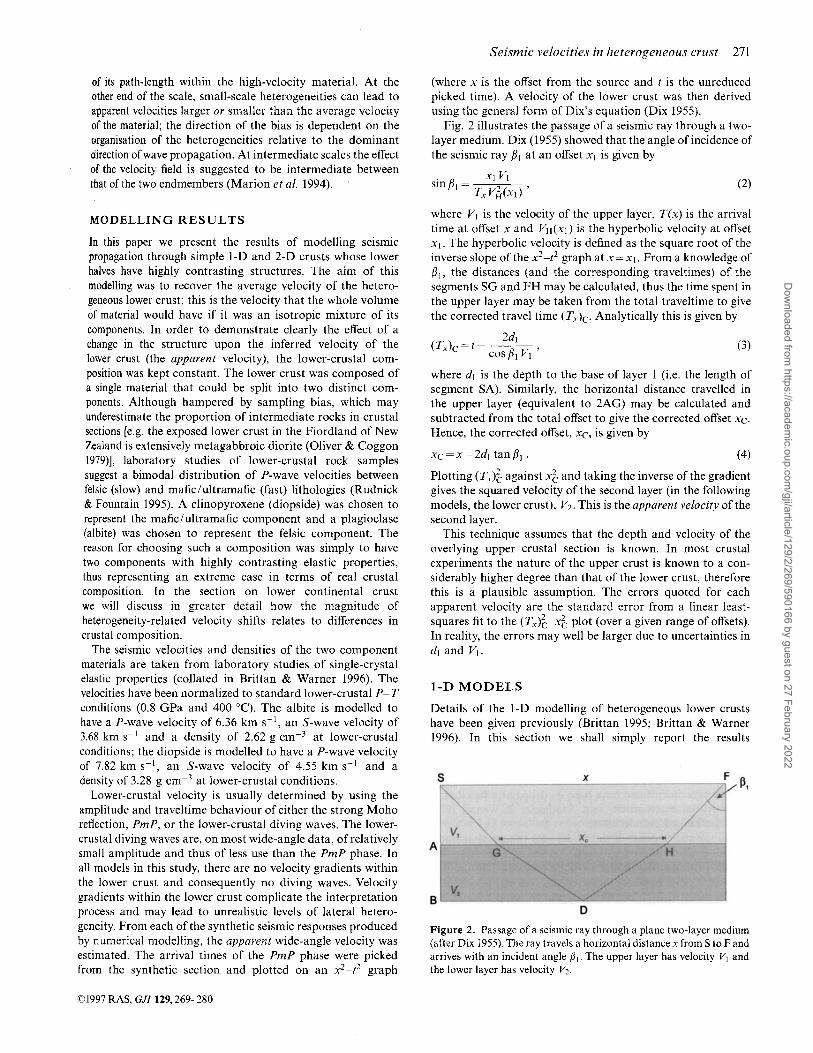
Fig. 2 illustrates the passage of a seismic ray through a two- layer medium. Dix (1955) showed that the angle of incidence of the seismic ray PI at an offset x1 is given by

where VI is the velocity of the upper layer, T(x) is the arrival time at offset x and VH(x1) is the hyperbolic velocity at offset X I . The hyperbolic velocity is defined as the square root of the inverse slope of the x2-t2 graph at x= X I . From a knowledge of PI, the distances {and the corresponding traveltimes) of the segments SG and FH may be calculated, thus the time spent in the upper layer may be taken from the total traveltime to give the corrected travel time (rx)c. Analytically this is given by

(3)

where dl is the depth to the base of layer 1 (i.e. the length of segment SA). Similarly, the horizontal distance travelled in the upper layer (equivalent to 2AG) may be calculated and subtracted from the total offset to give the corrected offset xc. Hence, the corrected offset, XC, is given by

xc=x-2dl tanp, . (4) Plotting (TJ: against x; and taking the inverse of the gradient gives the squared velocity of the second layer (in the following models, the lower crust), V2. This is the apparent velocity of the second layer.

This technique assumes that the depth and velocity of the overlying upper crustal section is known. In most crustal experiments the nature of the upper crust is known to a considerably higher degree than that of the lower crust, therefore this is a plausible assumption. The errors quoted for each apparent velocity are the standard error from a linear least- squares fit to the ( T x ) ~ - x ~ plot (over a given range of offsets). In reality, the errors may well be larger due to uncertainties in dl and Vl.

1-D MODELS

Details of the 1-D modelling of heterogeneous lower crusts have been given previously (Brittan 1995; Brittan & Warner 1996). In this section we shall simply report the results

S X

A

B D

Figure 2. Passage of a seismic ray through a plane two-layer medium (after Dix 1955). The ray travels a horizontal distance x from S to F and arrives with an incident angle P I . The upper layer has velocity V I and the lower layer has velocity Vz.

01997 RAS, GJI 129,269-280

Dow




important to this study. Three simple 1-D models were tested. The first model had a homogeneous lower crust; this is similar to the structure assumed in most forward modelling of wide- angle data. The second model had a lower crust with the bimodal composition arranged into horizontal layers. The layer width was of the same order of magnitude or larger than the investigating seismic wavelength, that is ka>> 1. The third model also has the bimodal composition, in this case arranged in' vertical layers. In contrast to the second model, the layer width is much less than the investigating seismic wavelength, that is k a c 1. The thin layers were replaced by an anisotropic equivalent medium. The geological justifications of models such as these are given later in this paper.

The synthetic seismic response of the first model showed two main phases on the seismogram, the wide-angle reflections from the top of the lower crust (labelled PcP) and the wide-angle Moho reflection (labelled PmP). The observed PmP traveltimes were picked, and using the technique described above an apparent lower-crustal velocity of 7.02 (kO.01) km s-' was derived (over an offset range of 100-400 km). This is identical to the average (Voigt-Reuss-Hill) velocity of the lower crust in the model.

The thick horizontal layers of the second crustal model affect the seismic wavefield in a significantly different manner. For oblique angles of incidence, the seismic wave will spend proportionally more of its travel path in the high-velocity layers and thus the resultant time-averaged velocity will move towards the higher velocity. In a thickly layered medium, the apparent velocity will not correctly reflect the average velocity. In the case of the thick layers it was very difficult to fit a straight line to the xc(Tx): graph at all offsets, that is finding an isotropic lower crust that will produce the measured traveltimes at all offsets was impossible. As heterogeneous crust of this nature is grossly anisotropic, the apparent velocity is clearly offset-dependent. It was shown that as the offset of the aperture increases, the apparent velocity increases. This is an effect of Fermat's Principle; at wide-angles, as the path length of the wave increases, the wave will spend more of its travel path in the fast layers. Calculating the apparent lower-crustal velocity for this model using the traveltimes from longer offsets (100-300 km) gave a velocity of 7.47 (k0.04) km s-'. The amplitude response of the second model was also considerably different from that with the isotropic, homogeneous lower crust. The amplitude of the Moho reflection decreases rapidly with offset as a large proportion of the energy is scattered incoherently by the large heterogeneities-this energy from the lower crust appears on each trace between the reflected waves from the Moho and from the top of the lower crust. Such reverbatory data have often been seen in wide-angle seismic experiments and have been modelled as a function of lower-crustal heterogeneity (e.g. Sandmeier & Wenzel 1986, 1990; Larkin & Levander 1995).

The seismic response of the model with thin vertical layers gave a traveltime of the PmP phase that was different from that of the corresponding phase in both previous 1-D models. Calculating the apparent lower-crustal velocity shows that signals reflected from the Moho appear to travel through the lower crust with the lowest velocity of the three models, 6.83 (k0.02) km s-' (over an offset range of 100400 km). This value confirms the results of Marion et al. (1994) as the wide-angle waves travel close to the axis of symmetry. The wave detected perpendicular to the dominant layering (in this

case the wave used to derive the apparent velocity) will be an organisation of energy from multiply scattered waves and will always have a velocity less than the average velocity of the two composite materials (Thomsen 1986).

2-D MODELLING

In the 2-D modelling we concentrated on investigating the seismic response of a large block of lower crust composed of heterogeneities that are large enough (in relation to the dominant seismic wavelength) to make equivalent media theory invalid and yet considerably smaller than the blocks typically modelled using ray theory (e.g. scale lengths less than around 20 km). This, however, presented a number of practical difficulties. In particular, adequate modelling in this regime requires the use of a complete wave solution in two dimensions (i.e. finite-difference or finite-element schemes) with a densely sampled grid of nodes covering the crustal section. To model a 165x22 km crustal section using the acoustic wave equation the model must be specified at approximately 1 .6~10 ' nodes, and using the elastic wave equation at approximately 1.7X1O6 nodes. It is therefore clearly impractical to use a deterministic approach to build the model (i.e. to individually locate heterogeneities by hand). A more feasible alternative is to build heterogeneous models whose characteristics (both in terms of physical properties such as velocity or density and the spatial organisation of these properties) can be parametrized using statistics. In stochastic modelling the aim is to reproduce some characteristic of the seismic response rather than to match the data exactly; the end goal is to find the gross statistical properties of the heterogeneous area (Bean & McCloskey 1995).

Previous studies of the nature of crustal heterogeneity have concentrated on matching synthetic data derived from stochastic modelling with actual field observations. For upper- crustal studies the field observations used have been well logs and the data from seismic experiments; for deeper areas the data modelled have tended to be earthquake data from large, widely spaced arrays. Three main forms of spatial distribution are commonly used to form a stochastic model: Gaussian, exponential and self-similar (or fractal) correlation functions. The nature and characteristics of the three distributions are discussed in detail in Frankel & Clayton (1986) and Holliger & Levander (1992) and will only be described briefly here. The 2-D Gaussian correlation function has the form

(5) where

r = / z .

The correlation length in the x-direction is a and the correlation length in the z-direction is b. The exponential spatial distribution is described by

C(r)=e-'. (6) Self-similar spatial distributions are described using the 2-D Von Karman correlation function

4nv2rYKV(r) C(r) =

K"(0) ' (7)

01997 RAS, GJI 129, 269-280

Dow




where K, is the modified Bessel function of order v and v is the Hurst number, which describes the fractal nature of the medium. For a Hurst number v = 0.5, the correlation function simplifies to the exponential correlation function. There are two interrelated important differences between the three distribution functions. First, for the Gaussian and exponential correlation functions the correlation length (a or b) is approximately the same as the dominant wavelength of the heterogeneities, while for self-similar media the correlation length is in effect the upper bound upon the fractal nature of the medium (Bean & McCloskey 1995). Heterogeneities in self-similar media can occur with sizes larger or smaller than correlation length, but only those smaller than it are fractal in nature. Second, self-similar distributions by their nature do not lose power at small wavelengths (high wave- numbers), unlike the corresponding Gaussian and exponential distributions.

A number of studies have attempted to find which of these three distribution functions produces the most accurate fit to data collected from the Earth. Bean & McCloskey (1995) argued that only a self-similar velocity distribution can account for both the reflectivity seen from upper-crustal bore- hole studies and the nature of wide-angle seismic data from the upper crust. Frankel & Clayton (1986) modelled the traveltime fluctuations across large seismic arrays and the codas from microearthquakes (f > 1 Hz). The best-fitting stochastic model to these data utilized a self-similar correlation function with a _+lo per cent standard deviation in velocity and a horizontal correlation distance greater than 10 km. Holliger & Levander (1992) digitized two geological sections through the Ivrea Zone, a section of exposed lower crust. The best fit to the spatial distribution of petrophysical properties was found to be a self-similar Von Karman function with Hurst number 0.3 and correlation lengths of around 700 m (horizontal) and 150 m (vertical). Holliger, Levander & Goff (1993) showed that a random lower crust with these properties and a bimodal velocity distribution would produce a seismic signature very similar to that often seen on deep seismic experiments. In general, the studies suggest that the crust can be best modelled using a self-similar correlation function. The lower crust in particular appears to have a ratio of horizontal to vertical correlation lengths of 3 : 1; however, the actual dominant correlation lengths present are unclear. The numbers given above are a strong function of sampling interval.

The 2-D media used in our modelling studies were generated using a linear stochastic process (Kerner 1994). The spread of P- and S-wave velocities and densities are described by a Gaussian distribution with user-specified mean and variance. The spatial arrangement of these parameters are described by a 2-D autocorrelation function representing their distribution in the x and z directions. The following is a simplified description of the process of constructing a random field for a particular parameter (e.g. P-wave velocity).

The first step is to assign a random function to the model grid to describe the parameter distribution. This takes the form of a Gaussian deviate with a zero mean and a variance of one. This function must then be filtered to provide a spatial arrangement with the required 2-D statistics. The statistics of the spatial distribution are described by autocorrelation functions in the x- and z-directions; the autocorrelation of a spatial series describes the similarity between that series and a spatially shifted version of itself. The 1-D

autocorrelation functions for the exponential and Gaussian spatial arrangements were given by a generalized Gaussian function (Tarantola 1987)

where r(.) is the gamma function, Lp is the correlation length and p describes the shape of the autocorrelation function. The two shapes of autocorrelation function used were the exponential function ( p = 1) and the Gaussian function ( p = 2). The Von Karman correlation function (eq. 7) was used to simulate a self-similar medium. A value of v = 0.3 was used for the Hurst number of the distribution.

As the filtering process involves the convolution of the 2-D spatial autocorrelation functions with the random parameter distribution, it is computationally more efficient to Fourier transform both functions and carry out the operation in the wavenumber (k) domain. The resulting filtered random function is then inversely transformed into the spatial domain and scaled as required by multiplication with the parameter standard deviation and addition of the chosen mean value.

This process produces a continuous field in the random variable with a parameter spread about a pre-determined mean with the chosen standard deviation. The statistics of the field can be entirely described in terms of the correlation length in the x-direction, a, the correlation length in the z-direction, b, the mean parameter value p, the standard deviation c and the type of autocorrelation function. To combat the influence upon the model of unrealistic parameter values from the tail ends of the distribution, a high/low cut-off is applied; usually any grid point whose parameter had a value greater than four times the field standard deviation was given the value of four times the standard deviation. A cut-off closer to the mean value than this would adversely affect the distribution statistics and was avoided.

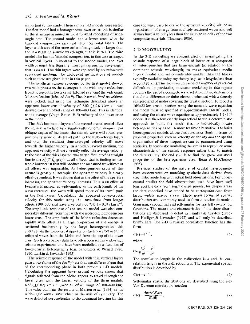
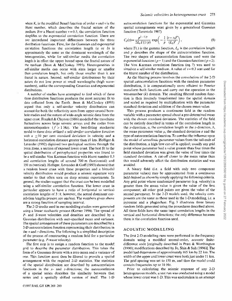
A binary field (i.e. a field with only two component parameter values) may be approximated from a continuous field derived as above by simply applying the following criteria. Any grid point whose randomized parameter (e.g. velocity) is greater than the mean value is given the value of the first component; all other grid points are given the value of the second parameter. In the 2-D models used, the velocity components are the same as those used in the 1-D modelling, i.e. a pyroxene and a plagioclase. Fig. 3 illustrates three binary random fields generated using the procedures described above. All three fields have the same input correlation lengths in the vertical and horizontal directions; the only difference between them is the correlation function used.

ACOUSTIC MODELLING

The first 2-D modelling runs were performed in the frequency domain using a modified second-order, acoustic finite- difference code [originally described in Pratt & Worthington (1990); modifications described by Jo, Shin & Suh (1996)l. The model had dimensions of approximately 165 km by 22 km. The width of the upper and lower crust were both just under 11 km. The grid spacing was set to 150 m, and thus the model could contain frequencies up to 10 Hz.

Prior to calculating the seismic response of any 2-D heterogeneous models, a test run was conducted using a model whose lower crust was 1-D. This was undertaken in an attempt

01997 RAS, GJI 129,269-280

Dow




I I 5i

I Average velocity of lower crust

I

Von Karman

$ z correlation length

x correlation length -*

Figure 3. Typical binary random fields used to represent the structure of the lower crust. Each of the three fields has a correlation length in the x direction of 3 km and a correlation length in the z direction of 0.75 km. The Von Karman model was created using a Hurst Number of 0.3.

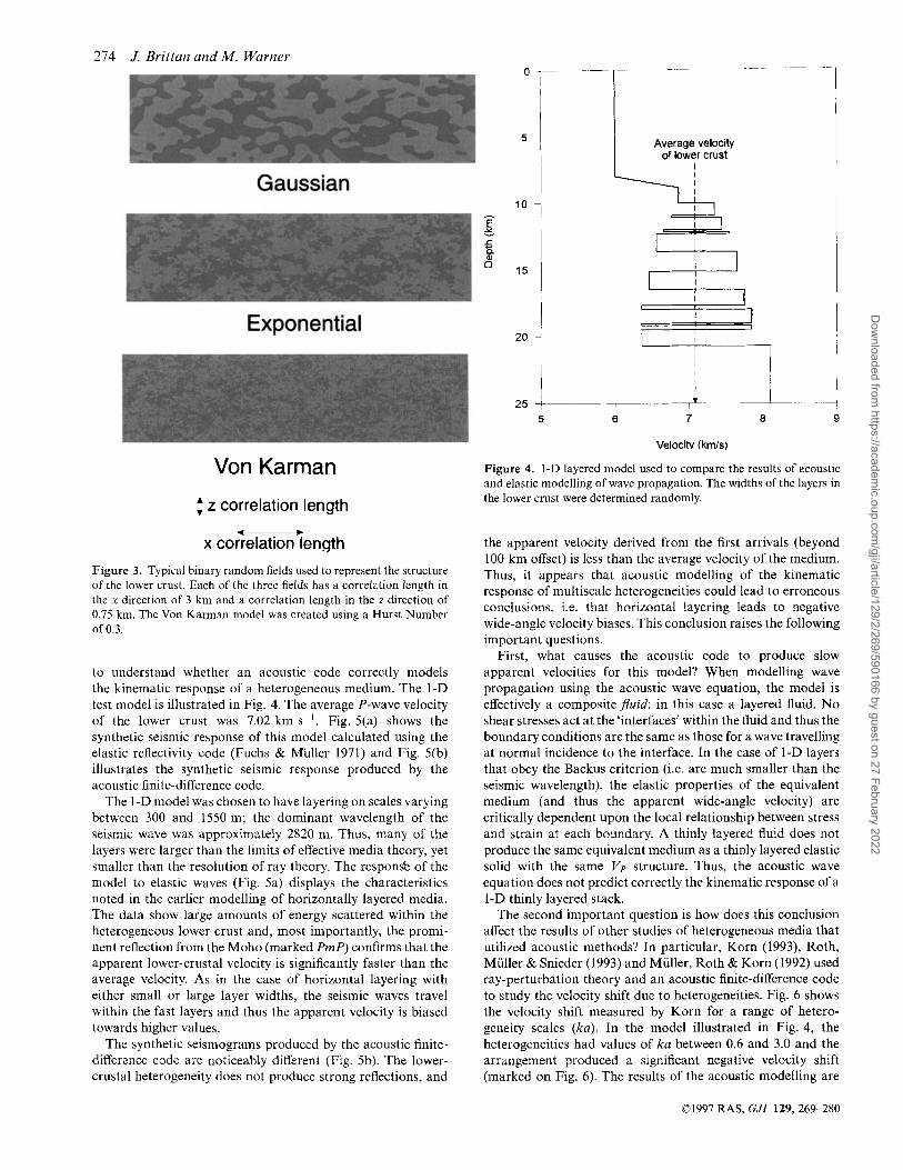
to understand whether an acoustic code correctly models the kinematic response of a heterogeneous medium. The 1-D test model is illustrated in Fig. 4. The average P-wave velocity of the lower crust was 7.02 km SK'. Fig. 5(a) shows the synthetic seismic response of this model calculated using the elastic reflectivity code (Fuchs & Muller 1971) and Fig. 5(b) illustrates the synthetic seismic response produced by the acoustic finite-difference code.

The 1-D model was chosen to have layering on scales varying between 300 and 1550 m; the dominant wavelength of the seismic wave was approximately 2820 m. Thus, many of the layers were larger than the limits of effective media theory, yet smaller than the resolution of ray theory. The responsk of the model to elastic waves (Fig. 5a) displays the characteristics noted in the earlier modelling of horizontally layered media. The data show large amounts of energy scattered within the heterogeneous lower crust and, most importantly, the promi- nent reflection from the Moho (marked PmP) confirms that the apparent lower-crustal velocity is significantly faster than the average velocity. As in the case of horizontal layering with either small or large layer widths, the seismic waves travel within the fast layers and thus the apparent velocity is biased towards higher values.

The synthetic seismograms produced by the acoustic finite- difference code are noticeably different (Fig. 5b). The lower- crustal heterogeneity does not produce strong reflections, and

I 20 -

I I I

I I I

I I

5 6 7 8 9

Velocitv (krn/s)

Figure 4. 1-D layered model used to compare the results of acoustic and elastic modelling of wave propagation. The widths of the layers in the lower crust were determined randomly.

the apparent velocity derived from the first arrivals (beyond 100 km offset) is less than the average velocity of the medium. Thus, it appears that acoustic modelling of the kinematic response of multiscale heterogeneities could lead to erroneous conclusions, i.e. that horizontal layering leads to negative wide-angle velocity biases. This conclusion raises the following important questions.

First, what causes the acoustic code to produce slow apparent velocities for this model? When modelling wave propagation using the acoustic wave equation, the model is effectively a compositejuid: in this case a layered fluid. No shear stresses act at the 'interfaces' within the fluid and thus the boundary conditions are the same as those for a wave travelling at normal incidence to the interface. In the case of 1-D layers that obey the Backus criterion (i.e. are much smaller than the seismic wavelength), the elastic properties of the equivalent medium (and thus the apparent wide-angle velocity) are critically dependent upon the local relationship between stress and strain at each boundary. A thinly layered fluid does not produce the same equivalent medium as a thinly layered elastic solid with the same V p structure. Thus, the acoustic wave equation does not predict correctly the kinematic response of a 1-D thinly layered stack.

The second important question is how does this conclusion affect the results of other studies of heterogeneous media that utilized acoustic methods? In particular, Korn (1993), Roth, Miiller & Snieder (1993) and Muller, Roth & Korn (1992) used ray-perturbation theory and an acoustic finite-difference code to study the velocity shift due to heterogeneities. Fig. 6 shows the velocity shift measured by Korn for a range of heterogeneity scales (ka). In the model illustrated in Fig. 4, the heterogeneities had values of ka between 0.6 and 3.0 and the arrangement produced a significant negative velocity shift (marked on Fig. 6). The results of the acoustic modelling are

01997 RAS, GJI 129, 269-280

Dow




1

f e -1

E

0 60 120 160

Distance (km)

1

2

3 0 40 80 7 20 160

Distance Ikm)

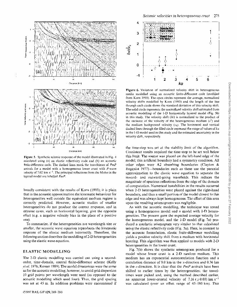
Figure 5. Synthetic seismic response of the model illustrated in Fig. 4 calculated using (a) an elastic reflectivity code and (b) an acoustic finite-difference code. The dashed lines mark the traveltimes of PmP arrivals for a model with a homogeneous lower crust with P-wave velocity of 7.02 km S S ' . The principal reflections from the Moho in the layered model are labelled PmP.

broadly consistent with the results of Korn (1993); it is plain that in the acoustic approximation the kinematic behaviour for heterogeneities well outside the equivalent medium regime is correctly predicted. However, acoustic studies of smaller heterogeneities do not produce the correct response, and in extreme cases, such as horizontal layering, give the opposite effect (e.g. a negative velocity bias in the place of a positive one).

To summarize, if the heterogeneities are wavelength size or smaller, the acoustic wave equation reproduces the kinematic response of the elastic medium incorrectly. Therefore, the following section describes the modelling of 2-D heterogeneities using the elastic wave equation.

ELASTIC MODELLING

The 2-D elastic modelling was carried out using a second- order, time-domain, central finite-difference scheme (Kelly et al. 1976; Kerner 1989). The model dimensions were the same as for the acoustic modelling; however, to avoid grid dispersion 10 grid points per wavelength were used (as opposed to the acoustic modelling which used four). Thus, the grid spacing was set at 45 m. In addition problems were encountered if

Y

1 - 7 7 7 + 1 2 3 4

ka

I

I 7-' 5 6

Figure 6 . Variation of normalized velocity shift in heterogeneous media modelled using an acoustic finite-difference code (modified from Korn 1993). The open circles represent the average, normalized velocity shifts modelled by Korn (1993) and the length of the line through each circle shows the standard deviation of this velocity shift. The solid circle represents the normalized velocity shift estimated from acoustic modelling of the I-D horizontally layered model (Fig. 5b) in this study. The velocity shift (6u) is normalized to the product of the variance of the velocity of the heterogeneous medium (6') and the medium background velocity (uo) . The horizontal and vertical dashed lines through the filled circle represent the range of values of ka in the 1-D model used in this study and the estimated uncertainty in the velocity shift, respectively.

the time-step was set at the stability limit of the algorithm. Consistent results required the time-step to be set well below this limit. The source was placed on the left-hand edge of the model; this artificial boundary had a symmetry condition. All other edges were A2 absorbing boundaries (Clayton & Engquist 1977)-boundaries such as these use the paraxial approximation to the elastic wave equation to separate the inward- and outward-going wavefields. This reduces the magnitude of spurious reflections from the edge of the domain of computation. Numerical instabilities in the results occurred when 2-D heterogeneities were placed against the right-hand boundary, and thus a small portion of the model closest to this edge and was always kept homogeneous. The effect of this area upon the resulting seismograms was negligible.

As with the acoustic modelling, the technique was tested using a homogeneous model and a model with 1-D heterogeneities. The process gave the expected average velocity for the homogeneous model, and the 1-D model (Fig. 7a) produced a synthetic seismogram very similar to that calculated using the elastic reflectivity code (Fig. 5a). Thus, in contrast to the acoustic formulation, elastic finite-difference modelling yields a positive velocity shift from a medium with horizontal layering. This algorithm was then applied to models with 2-D heterogeneities in the lower crust.

Fig. 7(b) shows the synthetic seismogram produced for a model whose lower crust is a 2-D random medium. This medium has an exponential autocorrelation function and a correlation distance of 9.0 km in the x-direction and 0.36 km in the z-direction. It is clear that the PmP arrivals have been shifted to earlier times by the heterogeneities; the traveltimes were picked and, using the method described earlier, an apparent lower-crustal velocity of 7.16 (k0.03) km SKI

was calculated (over an offset range of 45-160 km). This

01997 RAS, GJI 129,269-280

Dow




0 40 80 120 160

Distance (km)

0 10 80 120 160

Distance (kml

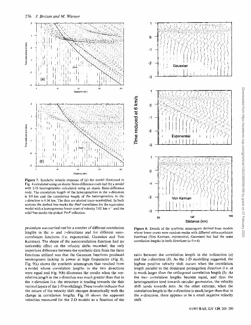
Figure 7. Synthetic seismic response of (a) the model illustrated in Fig. 4 calculated using an elastic finite-difference code and (b) a model with 2-D heterogeneities calculated using an elastic finite-difference code. The correlation length of the heterogeneities in the x-direction is 9.0 km and the correlation length of the heterogeneities in the z-direction is 0.36 km. The data are plotted trace-normalized. In both sections the dashed line marks the PmP traveltimes for the equivalent model with a homogeneous lower crust of velocity 7.02 km s-l and the solid line marks the picked PmP reflection.

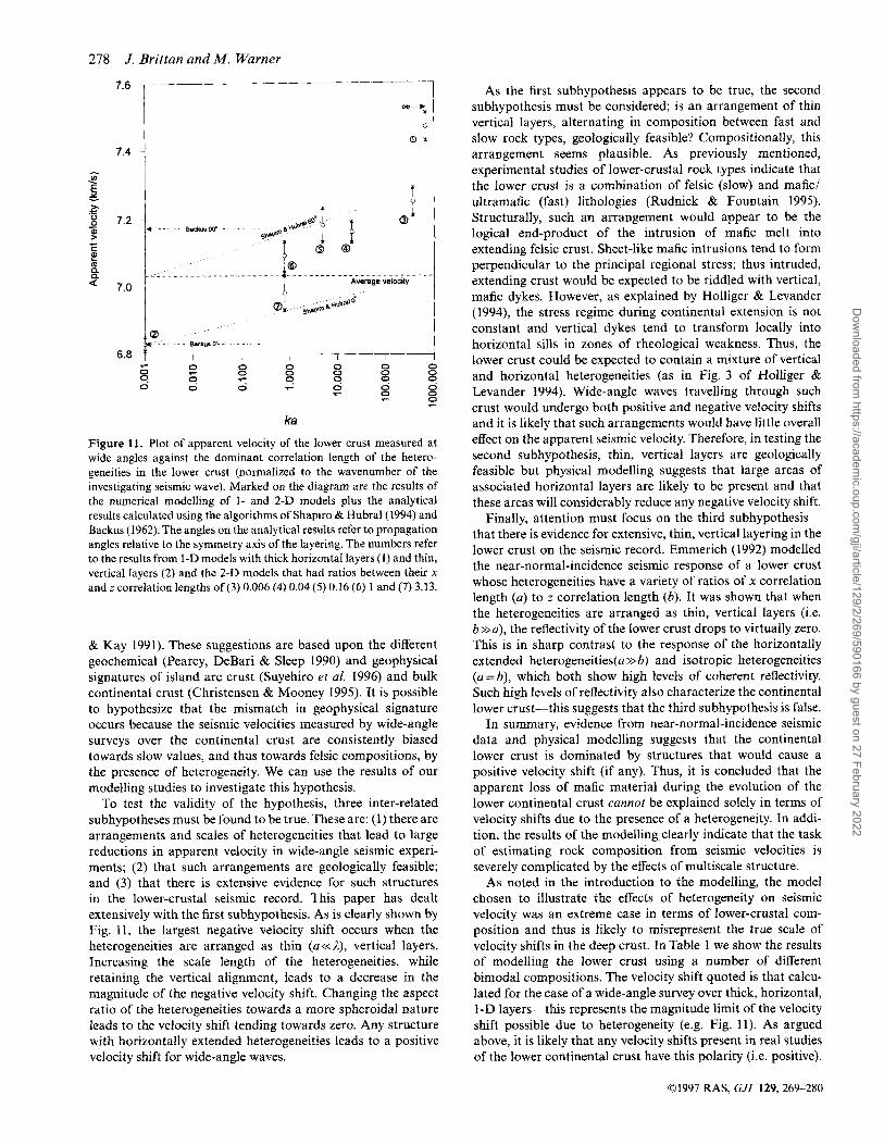
procedure was carried out for a number of different correlation lengths in the x- and z-directions and for different autocorrelation functions (i.e. exponential, Gaussian and Von Karman). The shape of the autocorrelation function had n o noticeable effect on the velocity shifts recorded; the only important difference between the synthetic data from the three functions utilized was that the Gaussian functions produced seismograms lacking in power at high frequencies (Fig. 8). Fig. 9(a) shows the synthetic seismogram that resulted from a model whose correlation lengths in the two directions were equal and Fig. 9(b) illustrates the results when the correlation length in the z-direction was much greater than that in the x-direction (i.e. the structure is tending towards the thin vertical layers of the I-D modelling). These results indicate that the nature of the velocity shift changes dramatically with the change in correlation lengths. Fig. 10 shows the apparent velocities measured for the 2-D models as a function of the

1

0

-1

-2

-3

1

r E

0 Y (0

rn n -1

3 TI

c.

8 E -2

i= E

-3

180 80 120

Distance (km)

Figure 8. Details of the synthetic seismogram derived from models whose lower crusts were random media with different autocorrelation functions (Von Karman, exponential, Gaussian) but had the same correlation lengths in both directions (a ib =4).

ratio between the correlation length in the x-direction (a) and the z-direction (b). As the 1-D modelling suggested, the highest positive velocity shift occurs when the correlation length parallel to the dominant propagation direction (i.e. a) is much larger than the orthogonal correlation length (b). As the two correlation lengths become equal, and thus the heterogeneities tend towards circular geometries, the velocity shift tends towards zero. At the other extreme, when the correlation length in the z-direction is much larger than that in the x-direction, there appears to be a small negative velocity shift.

01997 RAS, GJI 129, 269-280

Dow




m ; -1

2

3 0 40 80 120 160

Distance (km)

D

f ?

F E -1

2

3 40 80 I20 780

Distance (km)

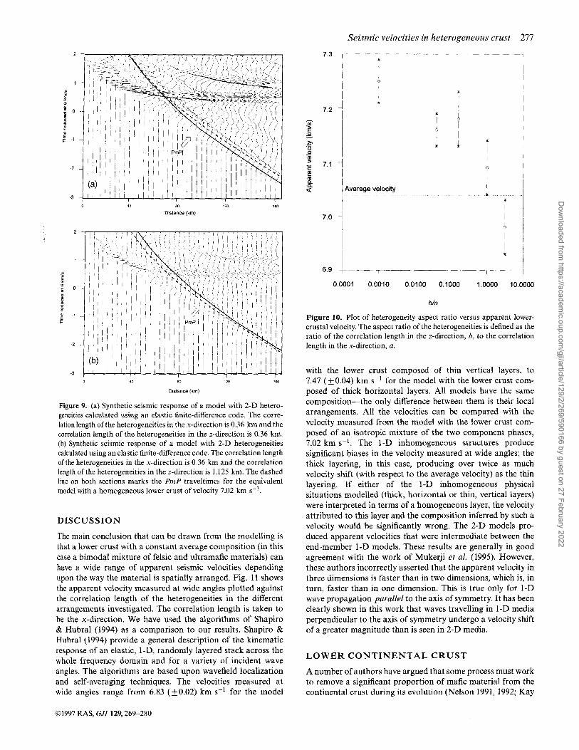
Figure 9. (a) Synthetic seismic response of a model with 2-D heterogeneities calculated using an elastic finite-difference code. The correlation length of the heterogeneities in the x-direction is 0.36 km and the correlation length of the heterogeneities in the z-direction is 0.36 km. (b) Synthetic seismic response of a model with 2-D heterogeneities calculated using an elastic finite-difference code. The correlation length of the heterogeneities in the x-direction is 0.36 km and the correlation length of the heterogeneities in the z-direction is 1.125 km. The dashed line on both sections marks the PmP traveltimes for the equivalent model with a homogeneous lower crust of velocity 7.02 km s-'.

DISCUSSION

The main conclusion that can be drawn from the modelling is that a lower crust with a constant average composition (in this case a bimodal mixture of felsic and ultramafic materials) can have a wide range of apparent seismic velocities depending upon the way the material is spatially arranged. Fig. 11 shows the apparent velocity measured at wide angles plotted against the correlation length of the heterogeneities in the different arrangements investigated. The correlation length is taken to be the x-direction. We have used the algorithms of Shapiro & Hubral (1994) as a comparison to our results. Shapiro & Hubral (1994) provide a general description of the kinematic response of an elastic, 1-D, randomly layered stack across the whole frequency domain and for a variety of incident wave angles. The algorithms are based upon wavefield localization and self-averaging techniques. The velocities measured at wide angles range from 6.83 (f0.02) km s-l for the model

7.3

7.2 - . u1

Y E Y

._ g - m

c 2 7.1 F a n a

7.0

6.9

t

\verage velocity

0.0001 0.0010 0.0100 0.1000 1.0000 10.0000

h/a

Figure 10. Plot of heterogeneity aspect ratio versus apparent lower- crustal velocity. The aspect ratio of the heterogeneities is defined as the ratio of the correlation length in the z-direction, b, to the correlation length in the x-direction, a.

with the lower crust composed of thin vertical layers, to 7.47 (k0.04) km s-' for the model with the lower crust composed of thick horizontal layers. All models have the same composition-the only difference between them is their local arrangements. All the velocities can be compared with the velocity measured from the model with the lower crust composed of an isotropic mixture of the two component phases, 7.02 km SK'. The 1-D inhomogeneous structures produce significant biases in the velocity measured at wide angles; the thick layering, in this case, producing over twice as much velocity shift (with respect to the average velocity) as the thin layering. If either of the 1-D inhomogeneous physical situations modelled (thick, horizontal or thin, vertical layers) were interpreted in terms of a homogeneous layer, the velocity attributed to this layer and the composition inferred by such a velocity would be significantly wrong. The 2-D models produced apparent velocities that were intermediate between the end-member 1-D models. These results are generally in good agreement with the work of Mukerji et al. (1995). However, these authors incorrectly asserted that the apparent velocity in three dimensions is faster than in two dimensions, which is, in turn, faster than in one dimension. This is true only for 1-D wave propagation parallel to the axis of symmetry. It has been clearly shown in this work that waves travelling in 1-D media perpendicular to the axis of symmetry undergo a velocity shift of a greater magnitude than is seen in 2-D media.

LOWER CONTINENTAL CRUST

A number of authors have argued that some process must work to remove a significant proportion of mafic material from the continental crust during its evolution (Nelson 1991, 1992; Kay

01997 RAS, GJI 129,269-280

Dow



218 J. Brittan and M . Warner

7.6 -7- 1

t l

. . 8.ctruv.. . . - 6.0 I I --7---7---T---

0 0

0 0

0 0 0 0 0 0 r 0

0 9 8 s 9 9 8 0 v

z z 0

s s F

&a

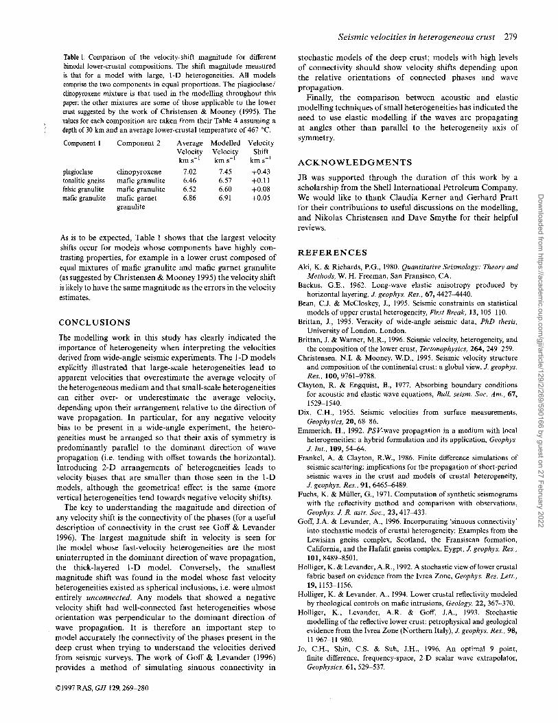
Figure 11. Plot of apparent velocity of the lower crust measured at wide angles against the dominant correlation length of the heterogeneities in the lower crust (normalized to the wavenumber of the investigating seismic wave). Marked on the diagram are the results of the numerical modelling of 1- and 2-D models plus the analytical results calculated using the algorithms of Shapiro & Hubral(l994) and Backus (1962). The angles on the analytical results refer to propagation angles relative to the symmetry axis of the layering. The numbers refer to the results from 1-D models with thick horizontal layers (1) and thin, vertical layers (2) and the 2-D models that had ratios between their x and z correlation lengths of (3) 0.006 (4) 0.04 ( 5 ) 0.16 (6) 1 and (7) 3.13.

& Kay 1991). These suggestions are based upon the different geochemical (Pearcy, DeBari & Sleep 1990) and geophysical signatures of island arc crust (Suyehiro et al. 1996) and bulk continental crust (Christensen & Mooney 1995). It is possible to hypothesize that the mismatch in geophysical signature occurs because the seismic velocities measured by wide-angle surveys over the continental crust are consistently biased towards slow values, and thus towards felsic compositions, by the presence of heterogeneity. We can use the results of our modelling studies to investigate this hypothesis.

To test the validity of the hypothesis, three inter-related subhypotheses must be found to be true. These are: (1) there are arrangements and scales of heterogeneities that lead to large reductions in apparent velocity in wide-angle seismic experiments; (2) that such arrangements are geologically feasible; and (3) that there is extensive evidence for such structures in the lower-crustal seismic record. This paper has dealt extensively with the first subhypothesis. As is clearly shown by Fig. 11, the largest negative velocity shift occurs when the heterogeneities are arranged as thin (a<< A), vertical layers. Increasing the scale length of the heterogeneities, while retaining the vertical alignment, leads to a decrease in the magnitude of the negative velocity shift. Changing the aspect ratio of the heterogeneities towards a more spheroidal nature leads to the velocity shift tending towards zero. Any structure with horizontally extended heterogeneities leads to a positive velocity shift for wide-angle waves.

As the first subhypothesis appears to be true, the second subhypothesis must be considered; is an arrangement of thin vertical layers, alternating in composition between fast and slow rock types, geologically feasible? Compositionally, this arrangement seems plausible. As previously mentioned, experimental studies of lower-crustal rock types indicate that the lower crust is a combination of felsic (slow) and mafic/ ultramafic (fast) lithologies (Rudnick & Fountain 1995). Structurally, such an arrangement would appear to be the logical end-product of the intrusion of mafic melt into extending felsic crust. Sheet-like mafic intrusions tend to form perpendicular to the principal regional stress; thus intruded, extending crust would be expected to be riddled with vertical, mafic dykes. However, as explained by Holliger & Levander (1994), the stress regime during continental extension is not constant and vertical dykes tend to transform locally into horizontal sills in zones of rheological weakness. Thus, the lower crust could be expected to contain a mixture of vertical and horizontal heterogeneities (as in Fig. 3 of Holliger & Levander 1994). Wide-angle waves travelling through such crust would undergo both positive and negative velocity shifts and it is likely that such arrangements would have little overall effect on the apparent seismic velocity. Therefore, in testing the second subhypothesis, thin, vertical layers are geologically feasible but physical modelling suggests that large areas of associated horizontal layers are likely to be present and that these areas will considerably reduce any negative velocity shift.

Finally, attention must focus on the third subhypothesis- that there is evidence for extensive, thin, vertical layering in the lower crust on the seismic record. Emmerich (1992) modelled the near-normal-incidence seismic response of a lower crust whose heterogeneities have a variety of ratios of x correlation length (a ) to z correlation length (b). It was shown that when the heterogeneities are arranged as thin, vertical layers (i.e. b>>a), the reflectivity of the lower crust drops to virtually zero. This is in sharp contrast to the response of the horizontally extended heterogeneities(a>>b) and isotropic heterogeneities (a=b), which both show high levels of coherent reflectivity. Such high levels of reflectivity also characterize the continental lower crust-this suggests that the third subhypothesis is false.

In summary, evidence from near-normal-incidence seismic data and physical modelling suggests that the continental lower crust is dominated by structures that would cause a positive velocity shift (if any). Thus, it is concluded that the apparent loss of mafic material during the evolution of the lower continental crust cannot be explained solely in terms of velocity shifts due to the presence of a heterogeneity. In addition, the results of the modelling clearly indicate that the task of estimating rock composition from seismic velocities is severely complicated by the effects of multiscale structure.

As noted in the introduction to the modelling, the model chosen to illustrate the effects of heterogeneity on seismic velocity was an extreme case in terms of lower-crustal composition and thus is likely to misrepresent the true scale of velocity shifts in the deep crust. In Table 1 we show the results of modelling the lower crust using a number of different bimodal compositions. The velocity shift quoted is that calculated for the case of a wide-angle survey over thick, horizontal, 1-D layers-this represents the magnitude limit of the velocity shift possible due to heterogeneity (e.g. Fig. 11). As argued above, it is likely that any velocity shifts present in real studies of the lower continental crust have this polarity (i.e. positive).

01997 RAS, GJI 129,269-280

Dow




Table 1. Comparison of the velocity-shift magnitude for different bimodal lower-crustal compositions. The shift magnitude measured is that for a model with large, 1-D heterogeneities. All models comprise the two components in equal proportions. The plagioclase/ clinopyroxene mixture is that used in the modelling throughout this paper; the other mixtures are some of those applicable to the lower crust suggested by the work of Christensen & Mooney (1995). The values for each composition are taken from their Table 4 assuming a depth of 30 km and an average lower-crustal temperature of 467 "C.

Component 1 Component 2 Average Modelled Velocity Velocity Velocity Shift km sK1 km s-' km s-l

plagioclase clinopyroxene 7.02 7.45 +0.43 tonalitic gneiss mafic granulite 6.46 6.57 +0.11 felsic granulite mafic granulite 6.52 6.60 +0.08 rnafic granulite mafic garnet 6.86 6.91 +0.05

~

granulite

As is to be expected, Table 1 shows that the largest velocity shifts occur for models whose components have highly contrasting properties, for example in a lower crust composed of equal mixtures of mafic granulite and mafic garnet granulite (as suggested by Christensen & Mooney 1995) the velocity shift is likely to have the same magnitude as the errors in the velocity estimates.

CONCLUSIONS

The modelling work in this study has clearly indicated the importance of heterogeneity when interpreting the velocities derived from wide-angle seismic experiments. The 1-D models explicitly illustrated that large-scale heterogeneities lead to apparent velocities that overestimate the average velocity of the heterogeneous medium and that small-scale heterogeneities can either over- or underestimate the average velocity, depending upon their arrangement relative to the direction of wave propagation. In particular, for any negative velocity bias to be present in a wide-angle experiment, the heterogeneities must be arranged so that their axis of symmetry is predominantly parallel to the dominant direction of wave propagation (i.e. tending with offset towards the horizontal). Introducing 2-D arrangements of heterogeneities leads to velocity biases that are smaller than those seen in the 1-D models, although the geometrical effect is the same (more vertical heterogeneities tend towards negative velocity shifts).

The key to understanding the magnitude and direction of any velocity shift is the connectivity of the phases (for a useful description of connectivity in the crust see Goff & Levander 1996). The largest magnitude shift in velocity is seen for the model whose fast-velocity heterogeneities are the most uninterrupted in the dominant direction of wave propagation, the thick-layered 1-D model. Conversely, the smallest magnitude shift was found in the model whose fast velocity heterogeneities existed as spherical inclusions, i.e. were almost entirely unconnected. Any models that showed a negative velocity shift had well-connected fast heterogeneities whose orientation was perpendicular to the dominant direction of wave propagation. It is therefore an important step to model accurately the connectivity of the phases present in the deep crust when trying to understand the velocities derived from seismic surveys. The work of Goff & Levander (1996) provides a method of simulating sinuous connectivity in

stochastic models of the deep crust; models with high levels of connectivity should show velocity shifts depending upon the relative orientations of connected phases and wave propagation.

Finally, the comparison between acoustic and elastic modelling techniques of small heterogeneities has indicated the need to use elastic modelling if the waves are propagating at angles other than parallel to the heterogeneity axis of symmetry.

ACKNOWLEDGMENTS

JB was supported through the duration of this work by a scholarship from the Shell International Petroleum Company. We would like to thank Claudia Kerner and Gerhard Pratt for their contributions to useful discussions on the modelling, and Nikolas Christensen and Dave Smythe for their helpful reviews.

REFERENCES

Aki, K. & Richards, P.G., 1980. Quantitative Seismology: Theory and Methods, W. H. Freeman, San Fransisco, CA.

Backus, G.E., 1962. Long-wave elastic anisotropy produced by horizontal layering, J. geophys. Rex , 67,44274440.

Bean, C.J. & McCloskey, J., 1995. Seismic constraints on statistical models of upper crustal heterogeneity, First Break, 13, 105-1 10.

Brittan, J., 1995. Veracity of wide-angle seismic data, PhD thesis, University of London, London.

Brittan, J. & Warner, M.R., 1996. Seismic velocity, heterogeneity, and the composition of the lower crust, Tectonophysics, 264,249-259.

Christensen, N.I. & Mooney, W.D., 1995. Seismic velocity structure and composition of the continental crust: a global view, J. geophys. Res., 100,9761-9788.

Clayton, R. & Engquist, B., 1977. Absorbing boundary conditions for acoustic and elastic wave equations, Bull. seism. SOC. Am., 67, 1529-1 540.

Dix, C.H., 1955. Seismic velocities from surface measurements, Geophysics, 20, 68-86.

Emmerich, H., 1992. PSV-wave propagation in a medium with local heterogeneities: a hybrid formulation and its application, Geophys. J. h i . , 109, 54-64.

Frankel, A. & Clayton, R.W., 1986. Finite difference simulations of seismic scattering: implications for the propagation of short-period seismic waves in the crust and models of crustal heterogeneity, J. geophys. Res., 91,6465-6489.

Fuchs, K. & Miiller, G., 1971. Computation of synthetic seismograms with the reflectivity method and comparison with observations, Geophys. J. R. astr. SOC., 23,417-433.

Goff, J.A. & Levander, A,, 1996. Incorporating 'sinuous connectivity' into stochastic models of crustal heterogeneity: Examples from the Lewisian gneiss complex, Scotland, the Fransiscan formation, California, and the Hafafit gneiss complex, Eygpt, J. geophys. Rex, 101,8489-8501.

Holliger, K. & Levander, A.R., 1992. A stochastic view of lower crustal fabric based on evidence from the Ivrea Zone, Geophys. Res. Lett., 19,1153-1156.

Holliger, K. & Levander, A., 1994. Lower crustal reflectivity modeled by rheological controls on mafic intrusions, Geology, 22, 367-370.

Holliger, K., Levander, A.R. & Goff, J.A., 1993. Stochastic modelling of the reflective lower crust: petrophysical and geological evidence from the Ivrea Zone (Northern Italy), J. geophys. Res., 98, 1 1 967-1 1 980.

Jo, C.H., Shin, C.S. & Suh, J.H., 1996. An optimal 9 point, finite difference, frequency-space, 2-D scalar wave extrapolator, Geophysics, 61,529-537.

01997 RAS, GJI 129,269-280

Dow




Kay, R.W. & Kay, S. Mahlburg., 1991. Creation and destruction of lower continental crust, Geol. Rundsch., 80, 259-278.

Kelly, K.R., Ward, R.W., Treitel, S. & Alford, R.M., 1976. Synthetic seismograms: a finite difference approach, Geophysics, 41,2-27.

Kerner, C., 1989. Simulation der Ausbreitung von seismischen Weleen in WellenKanaten mit der Methods der finiten Differenzen, in Proceedings of the 1984 Conferences on Cyber 200, pp. 83-1 10, ed. Ehlich, H., Universitaet Bochum, Bochum.

Kerner, C., 1994. Parameterization of 3D random media, in Modelling the Earth for Oil Exploration, pp. 333-338, ed., Helbig, K., Elsevier, Brussels.

Kerner, C.C. & Pratt, R.G., 1997. Effective media and velocity bounds of composites, Pure appl. Geophys., submitted.

Korn, M., 1993. Seismic waves in random media, J. appl. Geophys, 29, 247-269.

Larkin, S.P. & Levander, A., 1995. Path effects on deep crustal seismic data in the Basin and Range Province of the Western United States, EOS, Trans. Am. geophys. Un., 76, F400.

MacBeth, C., 1995. How can anisotropy be used for reservoir characterization?, First Break, 13, 31-37.

Marion, D., Mukerji, T. & Mavko, G., 1994. Scale effects on velocity dispersion: From ray to effective medium theories in stratified media, Geophysics, 59, 1613-1619.

Mooney, W.D. & Meissner, R., 1992. Multi-genetic origin of crustal reflectivity: continental lower crust and Moho, in ContinentalLower Crust, pp. 45-79, eds Fountain, D.M., Arculus, R. & Kay, R.W., Elsevier, Amsterdam.

Mukerji, T., Mavko, G., Mujica, D. & Lucet, N., 1995. Scale- dependent seismic velocity in heterogeneous media, Geophysics, 60, 1222- 1233.

Miiller, G., Roth, M. & Korn, M., 1992. Seismic traveltimes in random media, Geophys. J. Int., 110, 29-41.

Nelson, K.D., 1991. A unified view of craton evolution motivated by recent deep seismic reflection and refraction results, Geophys. J. Int., 105, 25-35.

Nelson, K.D., 1992. Are crustal thickness variations in old mountain belts like the Appalachians a consequence of lithospheric delamination?, Geology, 20,498-502.

Oliver, G.J.H. & Coggon, J.H., 1979. Crustal structure of Fiordland, New Zealand, Tectonophysics, 54, 253-292.

Pearcy, L.G., DeBari, S.M. & Sleep, N.H., 1990. Mass balance calculations for two sections of island arc crust and implications for the formation of continents, Earrh planet. Sci. Lett., 96, 427440.

Pratt, R.G. & Worthmgton, M.H., 1990. Acoustic wave equation inverse theory applied to multi-source cross-hole tomography, Part I: Acoustic wave-equation method, Geophys. Prospect.. 38, 311-330.

Roth, M., Miiller, G. & Snieder, R., 1993. Velocity shift in random media, Geophys. J. Int., 115, 552-563.

Rudnick, R.L. &Fountain, D.M., 1995. Nature and composition of the continental crust: a lower crustal perspective, Rev. Geophys., 33, 267-309.

Sadowiak, P., Meissner, R. & Brown, L., 1991. Seismic reflectivity patterns: comparative investigations of Europe and North America, in Continental Lithosphere: Deep Seismic Rejlections, eds Meissner, R., Brown, L., Diirbaum, H.-J., Franke, W., Fuchs, K. & Seifert, F., Am. geophys. Un. Geodyn. Ser., 22, 363-369.

Sandmeier, K.-J. & Wenzel, F., 1986. Synthetic seismograms for a complex crustal model, Geophys. Res. Lett., 13,22-25.

Sandmeier, K.-J. & Wenzel, F., 1990. Lower crustal petrology from wide-angle P- and S-wave measurements in the Black Forest, Tectonophysics, 173,495-505.

Shapiro, S.A. & Hubral, P., 1994. Generalized O’Doherty--Anstey formula for P-SV waves in random multilayered elastic media, Expanded abstracts 64th SEG Int. Mtng, 1426-1429.

Suyehiro, S. et al., 1996. Continental crust, crustal underplating and low-Q upper mantle beneath an oceanic island arc, Science, 272, 390-392.

Tarantola, A,, 1987. Inverse Problem Theory, pp. 26-28, Elsevier, Amsterdam.

Thomsen, L., 1986. Weak elastic anisotropy, Geophysics, 51, 1954-1966.

Walpole, L.J., 1981. Elastic behaviour of composite materials- Theoretical foundations, Advan. appl. Mech., 21, 169-242.

01997 RAS, GJI 129,269-280

Dow



wide-angle seismic velocities in heterogeneous crust - geophysical

Documents