when can history be our guide? the pitfalls of counterfactual inference

When Can History Be Our Guide?The Pitfalls of Counterfactual Inference1

GARY KING

Harvard University, Institute for Quantitative Social Science

LANGCHE ZENG

University of California-San Diego

Inferences about counterfactuals are essential for prediction, answering‘‘what if ’’ questions, and estimating causal effects. However, when thecounterfactuals posed are too far from the data at hand, conclusionsdrawn from well-specified statistical analyses become based on specu-lation and convenient but indefensible model assumptions rather thanempirical evidence. Unfortunately, standard statistical approaches as-sume the veracity of the model rather than revealing the degree ofmodel-dependence, so this problem can be hard to detect. We developeasy-to-apply methods to evaluate counterfactuals that do not requiresensitivity testing over specified classes of models. If an analysis fails thetests we offer, then we know that substantive results are sensitive to atleast some modeling choices that are not based on empirical evidence.We use these methods to evaluate the extensive scholarly literatures onthe effects of changes in the degree of democracy in a country (on anydependent variable) and separate analyses of the effects of UN peace-building efforts. We find evidence that many scholars are inadvertentlydrawing conclusions based more on modeling hypotheses than on ev-idence in the data. For some research questions, history contains insuf-ficient information to be our guide. Free software that accompanies thispaper implements all our suggestions.

Social science is about making inferencesFusing facts we know to learn about factswe do not know. Some inferential targets (the facts we do not know) are factual,which means that they exist even if we do not know them. In early 2003, SaddamHussein was obviously either alive or dead, but the world did not know which it was

Authors’ note: Thanks to Jim Alt, Scott Ashworth, Neal Beck, Jack Goldstone, Sander Greenland, Orit Kedar,Walter Mebane, Maurizio Pisati, Kevin Quinn, Jas Sekhon, Simon Jackman for helpful discussions; Michael Doyleand Nicholas Sambanis for their data and replication information; and the National Institutes of Aging (P01AG17625-01), the National Science Foundation (SES-0318275, IIS-9874747), and the Weatherhead Initiative for

research support.1 Easy-to-use software to implement the methods introduced here, called ‘‘WhatIf: Software for Evaluating

Counterfactuals,’’ is available at http://GKing.Harvard.edu/whatif; see Stoll, King, and Zeng (2006). At the sugges-tion of the editors, we minimized proofs and detailed mathematical arguments in this article and wrote a separatetechnical companion piece for Political Analysis that overlaps this one: it includes complete mathematical proofs,more general notation, and other methodological results not discussed here, but fewer examples and less peda-

gogical material; see King and Zeng (2006a). All information necessary to replicate the empirical results in this paperis available in King and Zeng (2006b).

r 2007 International Studies Association.Published by Blackwell Publishing, 350 Main Street, Malden, MA 02148, USA, and 9600 Garsington Road, Oxford OX4 2DQ, UK.

International Studies Quarterly (2007) 51, 183–210

until he was found. In contrast, other inferential targets are counterfactual, and thusdo not exist, at least not yet. Counterfactual inference is crucial for studying ‘‘whatif ’’ questions, such as whether the Americans and British would have invaded Iraqif the 9/11/2001 attack on the World Trade Center had not occurred. Counterfac-tuals are also crucial for making forecasts, such as whether there will be peace in theMideast in the next two years, as the quantity of interest is not knowable at the timeof the forecast but will eventually become known. Counterfactuals are essential aswell in making causal inferences, as causal effects are differences between factualand counterfactual inferences: for example, how much more international tradewould Syria have engaged in during 2003 if the Iraqi War had been averted?

Counterfactual inference has been a central topic of methodological discussion inpolitical science (Thorson and Sylvan 1982; Fearon 1991; Tetlock and Belkin 1996;Tetlock and Lebow 2001), psychology (Tetlock 1999; Tetlock, Lebow, and Parker2000), history (Murphy 1969; Dozois and Schmidt 1998; Tally 2000), philosophy(Lewis 1973; Kvart 1986), computer science (Pearl 2000), statistics (Rubin 1974;Holland 1986), and other disciplines. ‘‘Counterfactuals are an essential ingredientof scholarship. They help determine the research questions we deem importantand the answers we find to them’’ (Lebow 2000:558). As scholars have long rec-ognized, however, some counterfactuals are more amenable to empirical analysisthan others. In particular, some counterfactuals are more strained, farther from thedata, or otherwise unrealistic.

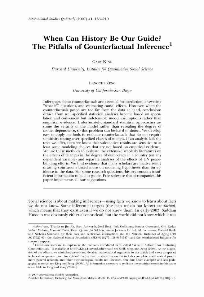
The problem is easy to see in the simple example in Figure 1. Here, we fit linearand quadratic models to a simple set of simulated data (with the one explanatoryvariable on the horizontal axis and the dependent variable and its expected valueon the vertical axis). The fit of the two models to the observed data is almostindistinguishable, and we have little statistical reason to choose one over the other.This is not a problem if we are interested in a prediction of Y for any X between 1and 2 where the data can be found; in this region, the choice of model is unim-portant as either model (or most any other model with a reasonably smooth func-tional form) would yield similar predictions. However, predictions of Y for values ofX outside the range of the data would be exquisitely sensitive to the choice of themodel. In other words, inferences in the range of the data are far less model-dependent than inferences outside the data. The risk with model-dependent infer-ences is that substantive conclusions are based more on apparently minor modelingchoices than on the empirical evidence.

Model 2: quadratic

0 1 2 3X

4 5 6

Model 1: linear

45

40

35

30

25

20

15

10

E (

YIX

)

5

0

−5

−10

FIG. 1. Linear and Quadratic Models With Equal Fit to Simulated Data But Massively DifferentOut-of-Sample Implications

When Can History Be Our Guide?184

But how can we tell how model-dependent our inferences are when the coun-terfactual inference is not so obviously extreme, or when the model involves morethan one explanatory variable? The answer to this question cannot come from anyof the model-based quantities we normally compute and our statistics programstypically report, such as standard errors, confidence intervals, coefficients, likeli-hood ratios, predicted values, test statistics, first differences, p-values, etc. (E.g.,although not shown in the figure, the confidence intervals for the extrapolations inFigure 1 do not contain the predictions from the other model for much of the rangeof the extrapolation.) To understand how far from the facts are our counterfactualinferences, and thus how model-dependent are our inferences, we need to lookelsewhere. At present, scholars study model-dependence primarily via sensitivityanalyses: changing the model and assessing how much conclusions change. If thechanges are substantively large for models in a particular class, then inferences aredeemed model-dependent. If the class of models examined are all a priori rea-sonable, and conclusions change a lot as the models within the class change, thenthe analyst may conclude that the data contain little or no information about thecounterfactual question at hand. This is a fine approach, but it is insufficient incircumstances where the class of possible models cannot be easily formalized andidentified, or where the models within a particular class cannot feasibly be enu-merated and run, that is, most of the time. In practice, the class of models chosenare those that are convenientFsuch as those with different control variables underthe same functional form. The identified class of models normally excludes at leastsome that have a reasonable probability of returning different substantive conclu-sions. Most often, this approach is skipped entirely.

What the approach offered here provides is several easy-to-apply methods thatreveal the degree of model dependency without having to run all the models. As aconsequence, it applies for the class of nearly all models, whether or not they areformalized, enumerated, and run, and for the class of all possible dependent vari-ables, conditional only on the choice of a set of explanatory variables. If an analysisfails our tests, then we know it will fail a sensitivity test too, but we avoid theimpossible position of having to run all possible models to find out.

Our field includes many discussions of the problem of strained counterfactuals inqualitative research. For example, Fearon (1991) and Lebow (2000) distinguish be-tween ‘‘miracle’’ and ‘‘plausible’’ counterfactuals and offer qualitative ways of judg-ing the difference. Tetlock and Belkin (1996: chapter 1) also discuss criteria forjudging counterfactuals (of which ‘‘historical consistency’’ may be of most relevanceto our analysis). Qualitative analysts seem to understand this issue well. Scholarsfrequently ask questions like whether the conflict in Iraq is sufficiently like Vietnamso that we can infer the outcome from this prior historical experience. Unfortu-nately, although the use of extreme counterfactuals is one of the most seriousproblems confronting comparative politics and international relations, quantitativeempirical scholarship rarely addresses the issue. Yet, it is hard to think of manyquantitative analysts in comparative politics and international relations in recentyears who do not hesitate to interpret their results by asking what happens, forexample, to the probability of conflict if all control variables are set to their meansand the key causal variable is changed from its 25th to its 75th percentile value(King, Tomz, and Wittenberg 2000). Every one of these analyses is making acounterfactual prediction, and every one needs to be evaluated by the same ideaswell known in qualitative research. In this paper, we provide quantitative measuresof these and related criteria that are meant to complement the ideas for qualitativeresearch discussed by many authors.

We offer two empirical examples. The first evaluates inferences in the scholarlyliteratures on the effects of democracy. These effects (on any of the dependentvariables used in the literature) have long been among the most studied questionsin comparative politics and international relations. Our results show that many

GARY KINGAND LANGCHE ZENG 185

analyses about democracy include at least some counterfactuals with little empiricalsupportFso that scholars in these literatures are asking some counterfactual ques-tions that are far from their data, and are therefore inadvertently drawing con-clusions about the effects of democracy in some cases based on indefensible modelassumptions rather than empirical evidence.

Whereas our example about democracy applies approximately to a large array ofprior work, we also introduce an example that applies exactly to one ground-breaking study on designing appropriate peacebuilding strategies (Doyle andSambanis 2000). We replicate this work, apply our methods to these data, and findthat the central causal inference in the study involves counterfactuals that are toofar from the data to draw reliable inferences, regardless of the methods employed.We illustrate by showing how inferences about the effect of UN intervention drawnfrom these data are highly sensitive to model specification.

The next section shows more specifically how to identify questions about thefuture and ‘‘what if ’’ scenarios that cannot be answered well in given data sets. Thissection introduces several new approaches for assessing how based in factual ev-idence is a given counterfactual. The penultimate section provides a new decom-position of the bias in estimating causal effects using observational data that is moresuited to the problems most prevalent in political science. This decomposition en-ables us to identify causal questions without good causal answers in given data setsand shows how to narrow these questions in some cases to those that can be an-swered more decisively. We use each of our methods to evaluate counterfactualsregarding the effects of democracy and UN peacekeeping. The last section con-cludes the article.

Forecasts and ‘‘What If ’’ Questions

Although statistical technology sometimes differs for making forecasts and estimat-ing the answers to ‘‘what if ’’ questions (e.g., Gelman and King 1994), the logic issufficiently similar that we consider them together. Although our suggestions aregeneral, we use aspects of the international conflict literature as a running exampleto fix ideas. Thus, let Y, our outcome variable, denote the degree of conflict initiatedby a country, and let X denote a vector of explanatory variables, including measuressuch as GDP and democracy. In regression-type modelsFincluding least squares,logit, probit, event counts, duration models, and most others used in the socialsciencesFwe usually compute forecasts and answers to ‘‘what if ’’ questions usingthe model-based conditional expected value of Y given a chosen vector of values x ofthe explanatory variables, X.

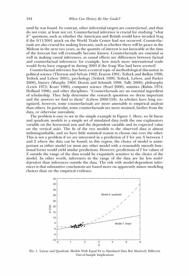
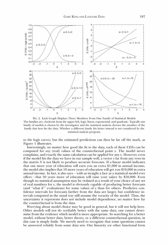
The model typically includes a specification for (i.e., assumption about) the con-ditional expectation function (CEF), which is merely a general expression for the linearor nonlinear regression line, that is, how the expected value (or mean) of Y dependson X. In linear regression, the CEF is EðY jXÞ ¼ Xb ¼ b0 þ b1X1 þ . . .þ bkXk,whereas in logistic regression the CEF is EðY jXÞ ¼ 1=ð1þ e�XbÞ. These CEFs andothers are illustrated in Figure 2 with one statistical model in each of four graphs,and with three CEFs displayed in each based on different choices of parametervalues from the chosen functional form. For example, the top right graph displaysonly the linear functional form, with three lines that differ based on their parametervalues (the intercept and slope). The task of the analyst is to choose the statisticalmodel (the graph), whereas the task of the parametric statistical analysis optimi-zation routine is to find the parameter values that select one member of the as-sumed family of curves that best fits the data. The optimization routines usuallywork exceptionally well, but they can only choose within the given family. If thedata are generated by one family of CEFs (one graph) but another is assumed bythe investigator, we will still get an approximation (such as the best linear approximation


to the logit curve), but the estimated predictions can then be far off the mark, asFigure 1 illustrates.

Interestingly, no matter how good the fit to the data, each of these CEFs can becomputed for any (real) values of the counterfactual point x. The model nevercomplains, and exactly the same calculation can be applied for any x. However, evenif the model fits the data we have in our sample well, a vector x far from any rows inthe matrix X is not likely to produce accurate forecasts. If a linear model indicatesthat one more year of education will earn you an extra $1,000 in annual income,the model also implies that 10 more years of education will get you $10,000 in extraannual income. In fact, it also saysFwith as straight a face as a statistical model everoffersFthat 50 years more of education will raise your salary by $50,000. Eventhough no statistical assumption may be violated as a result of your choice of any setof real numbers for x, the model is obviously capable of producing better forecasts(and ‘‘what if ’’ evaluations) for some values of x than for others. Predictive con-fidence intervals for forecasts farther from the data are larger, but confidence in-tervals computed in the usual way still assume the veracity of the model. Thus, theuncertainty it represents does not include model dependence, no matter how farthe counterfactual is from the data.

Worrying about model choice may be good in general, but it will not help here.Other models will not do verifiably better with the same data; one cannot deter-mine from the evidence which model is more appropriate. So searching for a bettermodel, without better data, better theory, or a different counterfactual question, inthis case is simply futile. We merely need to recognize that some questions cannotbe answered reliably from some data sets. Our linearity (or other functional form

−30.0

0.1

0.2

0.3

0.4

0.5

0.6

0.7

0.8

0.9

1.0

−2 −1 0 1 2 3 4

−3 −2 −1 0 1 2 3 4 −3 −2 −1 0 1 2 3 4

−3−3

−2

−1

0

0

4

8

12

16

20

24

28

0

4

8

12

16

20

24

28

32

36

40

1

2

3

4

−2 −1 0 1 2 3 4

a=0, b=2 a=.2, b=1

a=.1, b=.5

a=−.5, b=−.5a=0, b=−2

a=0, b=2

a=0, b=1.5

a=2.5, b=−.25 a=1, b=.75

a=1, b=−.75

a=0, b=1

a=0, b=2

E (

YIX

) =

logi

t (a+

bX)

E (

YIX

) =

(a+

bX)

E (

YIX

) =

ea+

bXE

(Y

IX)

= a+

bX

X

X X

X

FIG. 2. Each Graph Displays Three Members From One Family of Statistical ModelsThe families are, clockwise from the upper left, logit, linear, exponential, and quadratic. Typically onefamily of models is chosen by the investigator and the statistical analysis chooses the member of thefamily that best fits the data. Whether a different family fits better instead is not considered by the

statistical analysis program.


assumptions) are written globallyFfor any value of xFbut in fact are relevantonly locallyFin or near our observed data. In this paper, we are effectively seekingto understand where ‘‘local’’ ends and ‘‘global’’ begins. For forecasting and ana-lyzing what if questions, our task comes down to seeing how ‘‘far’’ x is from theobserved X.

Indeed, this point is crucial as the greater the distance from the counterfactual to theclosest reasonably sized portion of available data, the more model dependent inferences can beabout the counterfactual. In our technical companion paper, we define this claim moreprecisely and, apparently for the first time, prove it mathematically. That is, nomatter what the counterfactual, no matter what class of models one identifies asplausible, no matter how well the models tested fit the observed data, the fartherthe counterfactual from the data, the higher the degree of model dependencebecomes possible. Counterfactual questions sufficiently far from the data produceinferences with little or no empirical content. Moreover, our proof is highly general.It does not assume knowledge of the model, its functional form, the estimator, orthe dependent variable, and it only assumes that the CEF (conditional on X) satisfiesa general continuity condition, which fits almost all statistical models used andtheoretical processes hypothesized in the discipline.

We now offer two procedures for measuring the distance from a counterfactualto the data that can be used to assess whether a question posed can be reliablyanswered from any statistical model. Neither requires any information about themodel, estimator, or even the dependent variable.

Interpolation vs. Extrapolation

A simple but powerful distinction in measuring the distance of a counterfactualfrom the data, and thus assessing the counterfactual question x, is whether an-swering it by computing the CEF E(Y|x) would involve interpolation or extrapo-lation (e.g., Hastie, Tibshirani, and Friedman 2001; Kuo 2001). Except for someunusual situations for which we offer diagnostics below, data sets contain moreinformation about counterfactuals that require interpolation than those that re-quire extrapolation. Hence, answering a question involving extrapolation normallyrequires far more model-dependent inferences than one involving interpolation.

For intuition, imagine we have data on foreign aid received by countries with twonatural disasters in a year, and we wish to estimate how much foreign aid countriesreceive when they have two natural disasters in a year. (Suppose for simplicity thateach of the natural disasters is approximately the same size and of roughly the sameconsequence.) If we have enough such data, no modeling assumptions are neces-sary. That is, we can make a model-free inference by merely averaging the amountof money spent on foreign aid in these countries.

However, suppose we were still interested in foreign aid received by countrieswith two natural disasters, but we only observe countries with one or three disastersin a year. This is a simple (counterfactual) ‘‘what if ’’ question because we have nodata on countries with two natural disasters. The interpolation task, then, is to drawsome curve from expected foreign aid received in countries with a single naturaldisaster to the expected aid received in countries with three natural disasters;where it crosses the two-natural-disaster point is our inference. Without any as-sumptions, this curve could go anywhere, and the inferred amount of foreign aidreceived for countries with two disasters would not be constrained at all. Imposingthe assumption that the CEF is ‘‘smooth’’ (i.e., that it contains no sharp changes ofdirection and that it not bend too fast or too many times between the two endpoints) is quite reasonable for this example, as it is for most political science prob-lems; it is also intuitive, but it is stronger than necessary to prove our point. Theconsequence of this smoothness assumption is to narrow greatly the range of for-eign aid into which the interpolated value can fall, especially compared with an


extrapolation. Even if the aid received by countries with two disasters is higher thanthe aid received for countries with three disasters or lower than nations with onlyone, it probably will not be too much outside this range.

However, now suppose we observe the same data but need to extrapolate toforeign aid received for countries with four natural disasters. We could imposesome smoothness again, but even allowing one bend in the curve could make theextrapolation change a lot more than the interpolation. One way to look at this isthat the same level of smoothness (say the number of changes of direction allowed)constrains the interpolated value more than the extrapolated value, as for inter-polation any change in direction must be accompanied by a change back to intersectthe other observed point. With extrapolation, one change need not be matchedwith a change in the opposite direction, as there exists no observed point on theother side of the counterfactual being estimated. This is also an example of ourgeneral proof as the counterfactual requiring interpolation in this example is closerto more data than the counterfactual requiring extrapolation, so the interpolation isless model-dependent.

If we learn that a counterfactual question involves extrapolation, we still mightwish to proceed if the question is sufficiently important, but we would be aware ofhow much more model-dependent our answers will be. How to determine whethera question involves extrapolation with one variable should now be obvious. Ascer-taining whether a counterfactual requires extrapolation with more than one ex-planatory variable requires only one additional generalizing concept: Questionsthat involve interpolation are values of the vector x which fall in the convex hull of X.

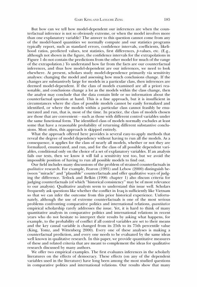
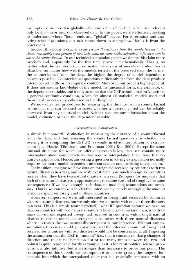
Formally, the convex hull of a set of points is the smallest convex set that containsthem. This is easiest to understand graphically, such as via the example in Figure 3for one explanatory variable (on the left) and for two (on the right), given simulateddata. The small vertical lines in the left graph denote data points on the oneexplanatory variable in that example. The convex hull for one variable is markedby the maximum and minimum data points: any counterfactual question betweenthose points requires interpolation; points outside involve extrapolation. (The leftgraph also includes a nonparametric density estimate, a smooth version of a histo-gram, that gives another view of the same data.) For two explanatory variables, the

−3−5

−4

−3

−2

−1

0

1

2

3

4

5

−5 −4 −3 −2 −1 0 1 2 3 4 50.0

0.1

0.2

0.3

0.4

0.5

−2 −1 0 1 2 3

P (

X)

X2

X X1

FIG. 3. Interpolation vs. Extrapolation: The Convex Hull of X is the Smallest Convex Set ThatContains the Data

Inference on points inside the convex hull requires interpolation, outside it requires extrapolation.With one explanatory variable, the convex hull is the interval between the minimum and the max-imum values of the observed data (as portrayed as the points farthest to the left and the right on theleft graph). With two explanatory variables, the convex hull is a polygon with vertices at the extremepoints of the data (as in the right graph). Neither graph portrays the dependent variable, as it is not

needed to ascertain whether the counterfactual is an interpolation or extrapolation.


convex hull is given by a polygon with extreme data points as vertices such that forany two points in the polygon, all points that are on the line connecting them arealso in the polygon (i.e., the polygon is a convex set). In other words, if the rightgraph in Figure 3 were a cork board, and the dots were nails, the convex hull wouldbe a rubber band stretched around all the points. With this definition of a convexhull, a counterfactual question x that appears outside the polygon requires ex-trapolation. Anything inside involves interpolation.

Although Figure 3 only portrays convex hulls for one and two explanatory vari-ables, the concept is well defined for any number of dimensions. For three ex-planatory variables, and thus three dimensions, the convex hull could be found by‘‘shrink wrapping’’ the fixed points in three dimensional space. The shrink-wrapped surface encloses counterfactual questions requiring interpolation. Forfour or more explanatory variables, the convex hull is more difficult to visualize,but from a mathematical perspective, the task of deciding whether a point lieswithin the hull generalizes directly.

The concept of a convex hull is well known in statistics and has been usedregularly to convey the idea of extrapolation and interpolation. However, it hasalmost never been used in practice for problems with more than a couple of ex-planatory variables. The problem is not conceptual but rather computational.Identifying the hull with even a few explanatory variables can take an extraordin-ary amount of computational power. Doing it with more than about 10 variablesappears nearly impossible. Moreover, the problem of locating whether a counter-factual point lies within or outside the hull is itself a difficult computational problemthat also has no solution known in the statistical literature.

In our technical companion paper, we solve this problem with a new algorithmcapable of quickly ascertaining whether a point lies within a convex hull even forlarge numbers of variables and data points. We have also developed easy-to-usesoftware, ‘‘WhatIf: Software for Evaluating Counterfactuals,’’ that automates thisconvex hull membership check as well as implements the other methods discussedin this paper (see Stoll, King, and Zeng, 2006). The result is that the convex hullcan now easily be used in any applied statistical analysis to sort counterfactualquestions that may be close enough to the data to be answered by the empiricalevidence from those that are farther away and may require more highly model-dependent inferences.

How Far Is the Counterfactual from the Data?

The interpolation vs. extrapolation distinction introduced in ‘‘Interpolation vs. ex-trapolation’’ is a simple dichotomous assessment of the distance from a counter-factual to the data. In our experience, this distinction is sufficient in most instancesto ascertain whether the data can support a counterfactual inference without ex-cessive model dependence. In some instances, however, a finer distinction is war-ranted. For example, points just outside the convex hull are arguably less of aproblem than those farther outside, and they are clearly closer to the data and, byour proof, less model dependent. Another related issue is that it is theoreticallypossible (although probably empirically infrequent) for a point just outside theinterpolation region defined by the convex hull of X to be closer to a large amountof data than one inside the hull that occupies a large empty region away from mostof the data. Thus, in addition to assessing whether a counterfactual question re-quires interpolation or extrapolation, we also more explicitly measure the distancefrom the counterfactual to the data.

Our goal here is some measure of the number or proportion of observations‘‘nearby’’ the counterfactual. To construct this quantity, we begin with a measure ofthe distance between two points (or rows) xi and xj based on Gower’s (1971) metric(which we call G2). It is defined simply as the average absolute distance between the


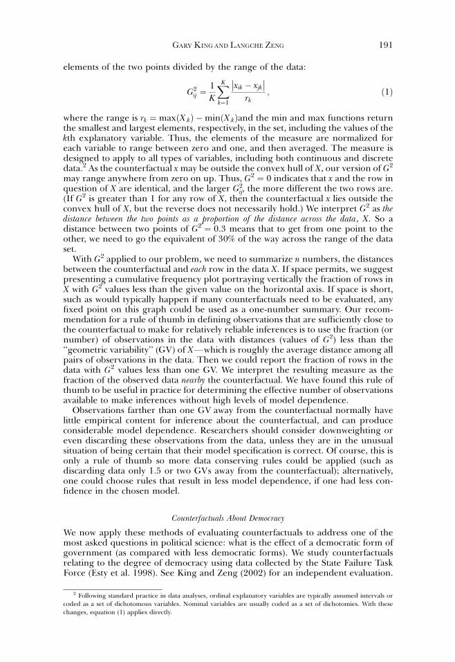
elements of the two points divided by the range of the data:

G2ij ¼

1

K

XK

k¼1

xik � xjk

�� rk

; ð1Þ

where the range is rk ¼ maxðX:kÞ �minðX:kÞand the min and max functions returnthe smallest and largest elements, respectively, in the set, including the values of thekth explanatory variable. Thus, the elements of the measure are normalized foreach variable to range between zero and one, and then averaged. The measure isdesigned to apply to all types of variables, including both continuous and discretedata.2 As the counterfactual x may be outside the convex hull of X, our version of G2

may range anywhere from zero on up. Thus, G2 ¼ 0 indicates that x and the row inquestion of X are identical, and the larger G2

ij, the more different the two rows are.(If G2 is greater than 1 for any row of X, then the counterfactual x lies outside theconvex hull of X, but the reverse does not necessarily hold.) We interpret G2 as thedistance between the two points as a proportion of the distance across the data, X. So adistance between two points of G2 ¼ 0.3 means that to get from one point to theother, we need to go the equivalent of 30% of the way across the range of the dataset.

With G2 applied to our problem, we need to summarize n numbers, the distancesbetween the counterfactual and each row in the data X. If space permits, we suggestpresenting a cumulative frequency plot portraying vertically the fraction of rows inX with G2 values less than the given value on the horizontal axis. If space is short,such as would typically happen if many counterfactuals need to be evaluated, anyfixed point on this graph could be used as a one-number summary. Our recom-mendation for a rule of thumb in defining observations that are sufficiently close tothe counterfactual to make for relatively reliable inferences is to use the fraction (ornumber) of observations in the data with distances (values of G2) less than the‘‘geometric variability’’ (GV) of XFwhich is roughly the average distance among allpairs of observations in the data. Then we could report the fraction of rows in thedata with G2 values less than one GV. We interpret the resulting measure as thefraction of the observed data nearby the counterfactual. We have found this rule ofthumb to be useful in practice for determining the effective number of observationsavailable to make inferences without high levels of model dependence.

Observations farther than one GV away from the counterfactual normally havelittle empirical content for inference about the counterfactual, and can produceconsiderable model dependence. Researchers should consider downweighting oreven discarding these observations from the data, unless they are in the unusualsituation of being certain that their model specification is correct. Of course, this isonly a rule of thumb so more data conserving rules could be applied (such asdiscarding data only 1.5 or two GVs away from the counterfactual); alternatively,one could choose rules that result in less model dependence, if one had less con-fidence in the chosen model.

Counterfactuals About Democracy

We now apply these methods of evaluating counterfactuals to address one of themost asked questions in political science: what is the effect of a democratic form ofgovernment (as compared with less democratic forms). We study counterfactualsrelating to the degree of democracy using data collected by the State Failure TaskForce (Esty et al. 1998). See King and Zeng (2002) for an independent evaluation.

2 Following standard practice in data analyses, ordinal explanatory variables are typically assumed intervals orcoded as a set of dichotomous variables. Nominal variables are usually coded as a set of dichotomies. With thesechanges, equation (1) applies directly.


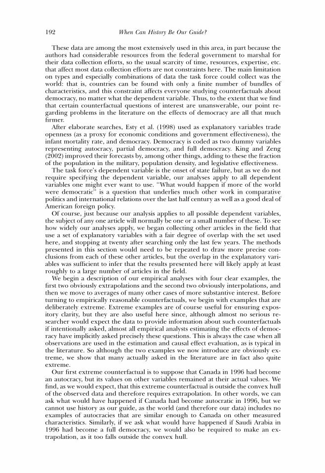
These data are among the most extensively used in this area, in part because theauthors had considerable resources from the federal government to marshal fortheir data collection efforts, so the usual scarcity of time, resources, expertise, etc.that affect most data collection efforts are not constraints here. The main limitationon types and especially combinations of data the task force could collect was theworld: that is, countries can be found with only a finite number of bundles ofcharacteristics, and this constraint affects everyone studying counterfactuals aboutdemocracy, no matter what the dependent variable. Thus, to the extent that we findthat certain counterfactual questions of interest are unanswerable, our point re-garding problems in the literature on the effects of democracy are all that muchfirmer.

After elaborate searches, Esty et al. (1998) used as explanatory variables tradeopenness (as a proxy for economic conditions and government effectiveness), theinfant mortality rate, and democracy. Democracy is coded as two dummy variablesrepresenting autocracy, partial democracy, and full democracy. King and Zeng(2002) improved their forecasts by, among other things, adding to these the fractionof the population in the military, population density, and legislative effectiveness.

The task force’s dependent variable is the onset of state failure, but as we do notrequire specifying the dependent variable, our analyses apply to all dependentvariables one might ever want to use. ‘‘What would happen if more of the worldwere democratic’’ is a question that underlies much other work in comparativepolitics and international relations over the last half century as well as a good deal ofAmerican foreign policy.

Of course, just because our analysis applies to all possible dependent variables,the subject of any one article will normally be one or a small number of these. To seehow widely our analyses apply, we began collecting other articles in the field thatuse a set of explanatory variables with a fair degree of overlap with the set usedhere, and stopping at twenty after searching only the last few years. The methodspresented in this section would need to be repeated to draw more precise con-clusions from each of these other articles, but the overlap in the explanatory vari-ables was sufficient to infer that the results presented here will likely apply at leastroughly to a large number of articles in the field.

We begin a description of our empirical analyses with four clear examples, thefirst two obviously extrapolations and the second two obviously interpolations, andthen we move to averages of many other cases of more substantive interest. Beforeturning to empirically reasonable counterfactuals, we begin with examples that aredeliberately extreme. Extreme examples are of course useful for ensuring expos-itory clarity, but they are also useful here since, although almost no serious re-searcher would expect the data to provide information about such counterfactualsif intentionally asked, almost all empirical analysts estimating the effects of democ-racy have implicitly asked precisely these questions. This is always the case when allobservations are used in the estimation and causal effect evaluation, as is typical inthe literature. So although the two examples we now introduce are obviously ex-treme, we show that many actually asked in the literature are in fact also quiteextreme.

Our first extreme counterfactual is to suppose that Canada in 1996 had becomean autocracy, but its values on other variables remained at their actual values. Wefind, as we would expect, that this extreme counterfactual is outside the convex hullof the observed data and therefore requires extrapolation. In other words, we canask what would have happened if Canada had become autocratic in 1996, but wecannot use history as our guide, as the world (and therefore our data) includes noexamples of autocracies that are similar enough to Canada on other measuredcharacteristics. Similarly, if we ask what would have happened if Saudi Arabia in1996 had become a full democracy, we would also be required to make an ex-trapolation, as it too falls outside the convex hull.


We now ask two counterfactual questions that are as obviously reasonable as thelast two were unreasonable. Thus, we ask what would have happened if Poland hadbecome an autocracy in 1990 (i.e., just after it became a democracy)? From quali-tative information available about Poland, this counterfactual is quite plausible, andmany even thought (and worried) it might actually occur at the time. Our analysisconfirms the plausibility of this suspicion as this question falls within the convexhull; analyzing it would require interpolation and probably not much model de-pendence. In other words, the world has examples of autocracies that are likePoland in all other measured respects, so history can be our guide. Another rea-sonable counterfactual is to ask what would have happened had Hungary become afull democracy in 1989 (i.e., just before it actually did become a democracy). Thisquestion is also in the convex hull and would therefore also require only inter-polation and little model dependence to draw inferences.

We now further analyze these four counterfactual questions using our modifiedGower distance measure. The question is how far the counterfactual x is from eachrow in the observed data set X, so the distance measure applied to the entire dataset gives n numbers. We summarize these numbers with our rule of thumb byasking what fraction of observations in our data are within one GV of G2, which isapproximately 0.1 (i.e., an average distance that is equivalent to 10% of the distancefrom the minimum to the maximum values on each variable in X). Essentially, noreal country-years are within 0.1 or less of this counterfactual for changing SaudiArabia to a democracy, but about 25% of the data are within this distance forHungary. Similarly, just a few observations in the data are within even 0.15 ofCanada changing to an autocracy, although about a quarter of the country-years arewithin this distance for Poland. Recall that we do not need all the data in ourcollection to be near a counterfactual, only as much as needed to base our infer-ences on.

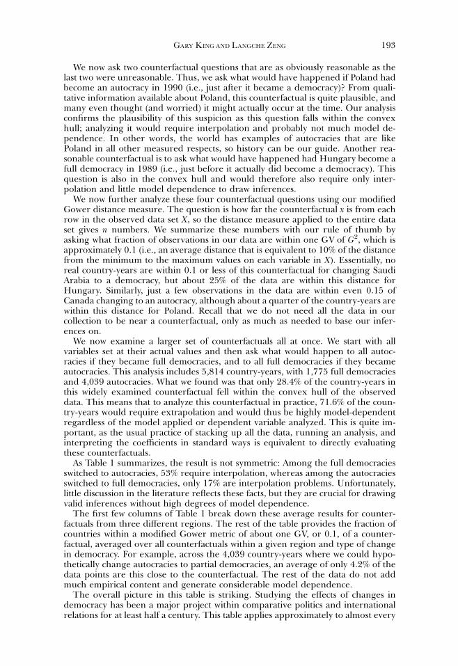
We now examine a larger set of counterfactuals all at once. We start with allvariables set at their actual values and then ask what would happen to all autoc-racies if they became full democracies, and to all full democracies if they becameautocracies. This analysis includes 5,814 country-years, with 1,775 full democraciesand 4,039 autocracies. What we found was that only 28.4% of the country-years inthis widely examined counterfactual fell within the convex hull of the observeddata. This means that to analyze this counterfactual in practice, 71.6% of the coun-try-years would require extrapolation and would thus be highly model-dependentregardless of the model applied or dependent variable analyzed. This is quite im-portant, as the usual practice of stacking up all the data, running an analysis, andinterpreting the coefficients in standard ways is equivalent to directly evaluatingthese counterfactuals.

As Table 1 summarizes, the result is not symmetric: Among the full democraciesswitched to autocracies, 53% require interpolation, whereas among the autocraciesswitched to full democracies, only 17% are interpolation problems. Unfortunately,little discussion in the literature reflects these facts, but they are crucial for drawingvalid inferences without high degrees of model dependence.

The first few columns of Table 1 break down these average results for counter-factuals from three different regions. The rest of the table provides the fraction ofcountries within a modified Gower metric of about one GV, or 0.1, of a counter-factual, averaged over all counterfactuals within a given region and type of changein democracy. For example, across the 4,039 country-years where we could hypo-thetically change autocracies to partial democracies, an average of only 4.2% of thedata points are this close to the counterfactual. The rest of the data do not addmuch empirical content and generate considerable model dependence.

The overall picture in this table is striking. Studying the effects of changes indemocracy has been a major project within comparative politics and internationalrelations for at least half a century. This table applies approximately to almost every


such analysis with democracy as an explanatory variable in every field with thesame or similar control variables, regardless of the choice of dependent variable.The results here appear to suggest that many inferences in these fields (or mostcountries within each analysis) have little information content for the questionsbeing posed and are highly model-dependent. Consequently, many conclusions arebased more on unverifiable assumptions about the model than on empirical data.The result varies by region and by counterfactuals, and it would of course varymore if we changed the set of explanatory variables. We can only really know forsure by applying the methods introduced here to these other data sets, but nomatter how you look at it, the problem of reaching beyond one’s necessarily limiteddata comes through in Table 1 with clarity.

Numerous interesting case studies could emerge from analyses like these. Forexample, public policy makers and the media spent considerable time debatingwhat would happen if Haiti became more of a democracy. In the early to mid-1990s, we find that the counterfactual of moving Haiti from a partial to a fulldemocracy was in the convex hull, and was a question that had a chance of beingaccurately answered with the available data. By 1996, conditions had worsened inthe country, and this counterfactual became more counter to the facts, moving wellout of the hull and thus required extrapolation.

Counterfactuals About UN Peacekeeping

In ‘‘the first quantitative analysis of the correlates of successful peacebuilding and ofthe contribution of UN operations to peacebuilding outcomes,’’ Doyle and Samb-anis (2000, 782) build and analyze a data set of 124 post-World War II civil wars.They characterize their results as firm enough to go beyond merely academicconclusions and to provide ‘‘broad guidelines for designing the appropriate peace-building strategy’’ (779) in practice. This work opens up a new area of quantitative

TABLE 1. How Factual Are Counterfactuals About Democracy?

Counterfactuals N % in Hull

Average % of Data ‘‘Nearby’’

All In Hull Only

Entire WorldFull Democracy to Autocracy 1,775 53.6% 5.5% 8.4%Autocracy to Full Democracy 4,039 17.6 2.4 8.2Part. Democracy to Autocracy 1,376 80.5 12.3 14.7Autocracy to Partial Democracy 4,039 61.8 4.2 6.0

Europe and Former USSRFull Democracy to Autocracy 961 54.9% 4.0% 5.8%Autocracy to Full Democracy 863 23.3 3.8 10.7Partial Democracy to Autocracy 493 86.0 11.2 12.7Autocracy to Partial Democracy 863 76.6 5.3 6.5

Canada and Latin AmericaFull Democracy to Autocracy 383 64.0 8.6 11.7Autocracy to Full Democracy 604 30.5 3.4 8.1Part. Democracy to Autocracy 328 81.7 11.9 13.9Autocracy to Partial Democracy 604 69.5 5.4 7.3

Other RegionsFull Democracy to Autocracy 431 40.4 5.9 11.6Autocracy to Full Democracy 2,572 12.8 1.7 6.4Partial Democracy to Autocracy 555 74.6 13.6 17.3Autocracy to Partial Democracy 2,572 55.0 3.5 5.4


analysis about an important public policy question for our field. We follow theirlead and study the authors’ ‘‘main concern’’F‘‘how international capacities, UNpeace operations in particular, influence the probability of peacebuilding success’’(783). Applying our methods, we found that the empirical conclusions offered inthe article on this issue depend mostly on statistical modeling assumptions ratherthan empirical evidence. We do not address the veracity of the article’s conclusions,only the weight of the data used to support them, and of course the authors shouldnot be faulted for being unaware of methods we introduce here, years after theirarticle was published. We also do not address the nine other hypotheses they test orother methodological issues raised by their analysis.

Doyle and Sambanis were helpful in providing us their data. We begin our anal-ysis by replicating their key logistic regression model, numbered A8 in their article(Doyle and Sambanis 2000: Table 3, p. 790). Other models (each with differentmeasures of UN intervention or other variables) in the article showed no effect ofany specific type of UN intervention considered. It was therefore only the finalspecification in their Model A8 that the authors offered to support the article’s keyconclusion that ‘‘multilateral United Nations peace operations make a positive dif-ference . . . and are usually successful in ending the violence’’ (abstract, p. 779).

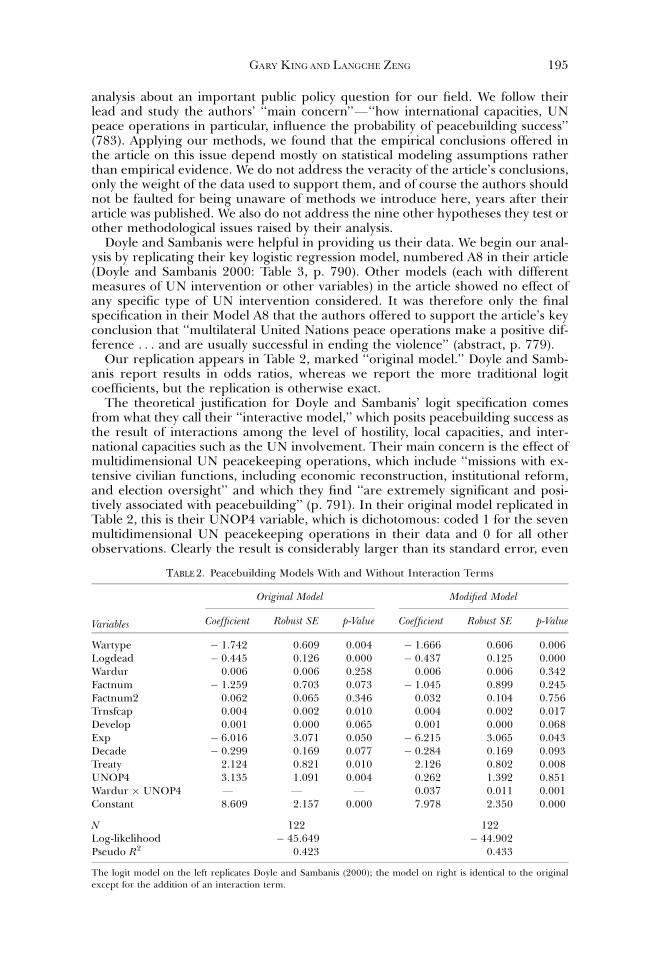
Our replication appears in Table 2, marked ‘‘original model.’’ Doyle and Samb-anis report results in odds ratios, whereas we report the more traditional logitcoefficients, but the replication is otherwise exact.

The theoretical justification for Doyle and Sambanis’ logit specification comesfrom what they call their ‘‘interactive model,’’ which posits peacebuilding success asthe result of interactions among the level of hostility, local capacities, and inter-national capacities such as the UN involvement. Their main concern is the effect ofmultidimensional UN peacekeeping operations, which include ‘‘missions with ex-tensive civilian functions, including economic reconstruction, institutional reform,and election oversight’’ and which they find ‘‘are extremely significant and posi-tively associated with peacebuilding’’ (p. 791). In their original model replicated inTable 2, this is their UNOP4 variable, which is dichotomous: coded 1 for the sevenmultidimensional UN peacekeeping operations in their data and 0 for all otherobservations. Clearly the result is considerably larger than its standard error, even

TABLE 2. Peacebuilding Models With and Without Interaction Terms

Variables

Original Model Modified Model

Coefficient Robust SE p-Value Coefficient Robust SE p-Value

Wartype � 1.742 0.609 0.004 � 1.666 0.606 0.006Logdead � 0.445 0.126 0.000 � 0.437 0.125 0.000Wardur 0.006 0.006 0.258 0.006 0.006 0.342Factnum � 1.259 0.703 0.073 � 1.045 0.899 0.245Factnum2 0.062 0.065 0.346 0.032 0.104 0.756Trnsfcap 0.004 0.002 0.010 0.004 0.002 0.017Develop 0.001 0.000 0.065 0.001 0.000 0.068Exp � 6.016 3.071 0.050 � 6.215 3.065 0.043Decade � 0.299 0.169 0.077 � 0.284 0.169 0.093Treaty 2.124 0.821 0.010 2.126 0.802 0.008UNOP4 3.135 1.091 0.004 0.262 1.392 0.851Wardur � UNOP4 F F F 0.037 0.011 0.001Constant 8.609 2.157 0.000 7.978 2.350 0.000

N 122 122Log-likelihood � 45.649 � 44.902Pseudo R2 0.423 0.433

The logit model on the left replicates Doyle and Sambanis (2000); the model on right is identical to the originalexcept for the addition of an interaction term.


given the small number of observations available. When translated into an oddsratio, which is Doyle and Sambanis’ preferred form, the odds of peacebuildingsuccess with a multidimensional UN peacekeeping operation is 23 times larger thanwith no such operation, holding constant a list of potential confounding controlvariables. We return to this remarkable result in ‘‘Identifying multivariate ex-trapolation regions with the convex hull’’ when we discuss causal inferences.

In this section, we examine the counterfactuals of interest. Assessing the causaleffects of multidimensional UN peacekeeping operations implicitly involves askingthe following question: In civil wars with multilateral UN involvement, how muchpeacebuilding success would we have witnessed if the UN had not gotten involved?Similarly, in civil wars without UN involvement, how much success would therehave been if the UN had gotten involved? In other words, the goal is counterfactualpredictions with the dichotomous UNOP4 variable set to 1FUNOP4, which is onecounterfactual for each observation. To begin with, we check how many counter-factuals are in the convex hull of the observed data. We found none. That is, everysingle counterfactual in the data set is a risky extrapolation rather than what wouldhave been a comparatively safer interpolation. We also computed the Gower dis-tance of each counterfactual from the data and found that few of the counterfac-tuals were near much of the data. For example, for all counterfactuals, an averageof only 1.3% of the observations were within one GV (which is 0.11 in these data).Thus, not only are the counterfactuals all extrapolations, but in addition they donot lie just outside the convex hull. Instead, most are fairly extreme extrapolationswell beyond the data. These results strongly indicate that the data used in the studycontain little information to answer the key causal question asked, and hence, theconclusions reached there are based more on theory and model specifications thanempirical evidence.

We now proceed to give relatively simple examples of the consequences of thisresult in terms of model dependence. We begin by making only one change in thelogit specification by including a simple interaction between UNOP4 and the du-ration of the civil war, leaving the rest of the specification as is. (This is of courseonly one illustrative example, and not the only aspect of the specification sensitiveto assumptions.) Including this interaction would seem highly consistent with the‘‘interactive’’ theory put forward in the article, so it would not seem possible toexclude on theoretical grounds alone. Excluding this interaction, which the originalspecification does, is equivalent to assuming that the effect of UN peacekeepingoperations is identical for wars of all durations (except for the trivial assumednonlinearities due to the logit model). Unfortunately, nothing in the theory ex-pounded in the article, or in other literature in the field, justifies the use of such anassumption without empirical testing.

The result of this new specification is given in the second set of columns in Table2. The coefficient on the interaction is positive and clearly distinguishable from zero(the p-value is 0.001), with a slightly higher likelihood and pseudo R2 values, rep-resenting clear evidence by the usual rules of thumb to indicate that this modelmight even be preferred to the original one. To be clear, however, we do notnecessarily favor this model or the original; we present both as two of many plau-sible alternatives not ruled out on the grounds of theory or data fitting. Moreover,no appropriate theory of statistical inference or analysis suggests whether to use theoriginal or modified model to draw inferences without empirical testing. Thus, weconsider the decision about whether to estimate the coefficient on the interaction ascompared with fixing it to zero (or, equivalently, excluding it) as an apparentlyminor specification decision and now show how remarkably sensitive inferences areto this choice.

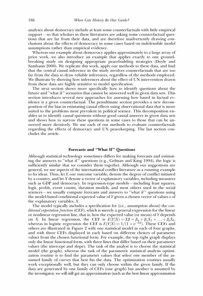
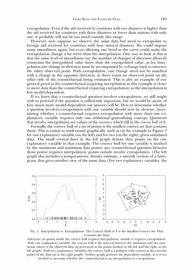
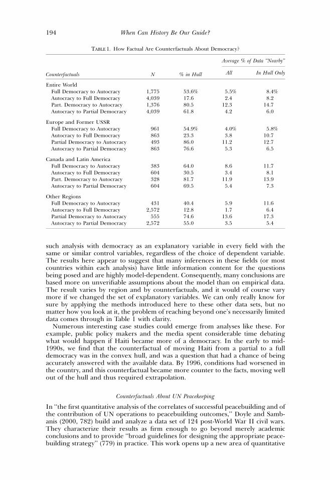
We now offer the left graph in Figure 4, which plots predicted values from bothmodels based on the actual values of UNOP4 and the other explanatory variables.This graph shows that almost all the predicted values from the two models fall on


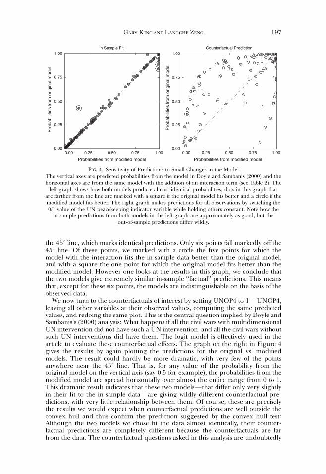
the 451 line, which marks identical predictions. Only six points fall markedly off the451 line. Of these points, we marked with a circle the five points for which themodel with the interaction fits the in-sample data better than the original model,and with a square the one point for which the original model fits better than themodified model. However one looks at the results in this graph, we conclude thatthe two models give extremely similar in-sample ‘‘factual’’ predictions. This meansthat, except for these six points, the models are indistinguishable on the basis of theobserved data.

We now turn to the counterfactuals of interest by setting UNOP4 to 1�UNOP4,leaving all other variables at their observed values, computing the same predictedvalues, and redoing the same plot. This is the central question implied by Doyle andSambanis’s (2000) analysis: What happens if all the civil wars with multidimensionalUN intervention did not have such a UN intervention, and all the civil wars withoutsuch UN interventions did have them. The logit model is effectively used in thearticle to evaluate these counterfactual effects. The graph on the right in Figure 4gives the results by again plotting the predictions for the original vs. modifiedmodels. The result could hardly be more dramatic, with very few of the pointsanywhere near the 451 line. That is, for any value of the probability from theoriginal model on the vertical axis (say 0.5 for example), the probabilities from themodified model are spread horizontally over almost the entire range from 0 to 1.This dramatic result indicates that these two modelsFthat differ only very slightlyin their fit to the in-sample dataFare giving wildly different counterfactual pre-dictions, with very little relationship between them. Of course, these are preciselythe results we would expect when counterfactual predictions are well outside theconvex hull and thus confirm the prediction suggested by the convex hull test:Although the two models we chose fit the data almost identically, their counter-factual predictions are completely different because the counterfactuals are farfrom the data. The counterfactual questions asked in this analysis are undoubtedly

Counterfactual PredictionIn Sample Fit

Pro

babi

litie

s fr

om o

rigin

al m

odel

Pro

babi

litie

s fr

om o

rigin

al m

odel

Probabilities from modified modelProbabilities from modified model

0.000.00

0.25

0.50

0.75

1.00

0.00

0.25

0.50

0.75

1.00

0.25 0.50 0.75 1.000.00 0.25 0.50 0.75 1.00

FIG. 4. Sensitivity of Predictions to Small Changes in the ModelThe vertical axes are predicted probabilities from the model in Doyle and Sambanis (2000) and thehorizontal axes are from the same model with the addition of an interaction term (see Table 2). The

left graph shows how both models produce almost identical probabilities; dots in this graph thatare farther from the line are marked with a square if the original model fits better and a circle if themodified model fits better. The right graph makes predictions for all observations by switching the0/1 value of the UN peacekeeping indicator variable while holding others constant. Note how the

in-sample predictions from both models in the left graph are approximately as good, but theout-of-sample predictions differ wildly.


very important, but this analysis demonstrates that they cannot be reliably ad-dressed by the data used.

We return to the analysis of these data, as well as the massively different sub-stantive implications of these results, in ‘‘Identifying Multivariate ExtrapolationRegions with the Convex Hull.’’

Causal Inference

We now turn to causal inference and the counterfactual evaluation necessary as partof causal inference. We start with a definition of causal effects, and then our de-composition of the bias in estimation, and finally a discussion of the components ofbias. We devote the most space to discussing the components of bias due to inter-polation and extrapolation, during which we show how the techniques introducedin the previous section can also help solve an existing problem in causal inference.We illustrate with analyses in the same data used in ‘‘Counterfactuals about UNpeacekeeping’’ on UN peacekeeping.

Causal Effects Definition

To fix ideas, we use as a running example a version of the democratic peace hy-pothesis, which holds that democratic dyads are less conflictual than other dyads.Let D denote the ‘‘treatment’’ (or ‘‘key causal’’) variable where D ¼ 1 denotes ademocratic dyad and D ¼ 0 denotes a nondemocratic dyad. The dependent vari-able is Y, the degree of conflict (but our discussion generalizes to all other depend-ent variables too).

To define the causal effect of democracy on conflict, denote Y1 as the degree ofconflict that would be observed if the dyad contained two democracies and Y0 as thedegree of conflict if this dyad were not both democracies. Obviously, only either Y0

or Y1 but not both are observed for any one dyad at any given time, as (in ourpresent simplified formulation) a dyad either is or is not democratic. This is knownas the fundamental problem of causal inference (King, Keohane, and Verba 1994).

In principle, the democracy variable can have a different causal effect for everydyad in the sample. We can then define the causal effect of democracy by averagingover all dyads, or for the democratic and nondemocratic dyads separately (or forany other subset of dyads). For democratic dyads, this is known as the ‘‘averagecausal effect among the treated,’’ which we define as follows:

y ¼ EðY1jD ¼ 1Þ � EðY0jD ¼ 1Þ¼ ‘‘Factual’’� ‘‘Counterfactual’’

ð2Þ

We call the first termFthe average level of conflict among democratic dy-adsFfactual as Y1 is observable when D ¼ 1. We refer to the second as counter-factual because Y0Fthe degree of conflict that would exist in a dyad if it were notdemocraticFis not observed and indeed is unobservable in democratic dyads(D ¼ 1). (The causal effect for nondemocratic dyads (D ¼ 0) is directly analogousand also involves factual and counterfactual terms.)

Although medical researchers are usually interested in the average causal effectamong the treated y, political scientists are also interested in the average causaleffect for the entire set of observations,

g ¼ EðY1Þ � EðY0Þ; ð3Þwhere both terms in this equation have a counterfactual element, as each expect-ation is taken over all dyads; however, Y1 is only observed for democratic dyads andY0 only for nondemocratic dyads. These definitions of causal effects are used in awide variety of literatures (Rubin 1974; Holland 1986; King, Keohane, and Verba1994; Robins 1999a, 1999b; Pearl 2000).


A counterfactual x in this context, therefore, takes the form of some observeddata with only one element changedFfor example, the Mexico–Spain dyad with allits attributes fixed but with the regime type in both changed to autocracy. Ofcourse, we can easily evaluate how reasonable it is to ask about this counterfactual inone’s data with the methods already introduced in the previous section: Checkingwhether x falls in the convex hull of the observed X and computing the distancefrom x to X. In addition, as x has only one counterfactual element, we show that wecan easily consult another criterion, whether x falls on the support of X, although wediscuss some problems with this alternative in ‘‘Extrapolation Bias.’’ The support ofX is the range of values of X that are possible (i.e., have positive density) whether ornot they occur in our data.

In real applications, the true causal effect, y or g, is unknown and needs to beestimated. In ‘‘Bias Decomposition,’’ we discuss the sources of potential problems inusing observational data to estimate these causal effects. We focus on y there forexpository purposes, as is usual in the statistical and econometric literature. How-ever, unlike prior literature, our companion paper includes proofs that are gen-eralized to accommodate these quantities of interest to political science to show thatour results also hold for the effect on nondemocracies and for the overall averagetreatment effect, g, as well.

Bias Decomposition

We begin with the simplest estimator of y using observational data, the differencein means (or, equivalently, the coefficient on D from a regression of Y on a constantand D):

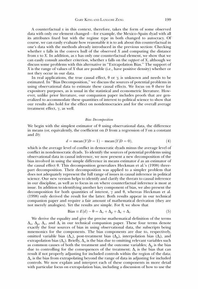
d ¼ meanðY jD ¼ 1Þ �meanðY jD ¼ 0Þ; ð4Þwhich is the average level of conflict in democratic dyads minus the average level ofconflict in nondemocratic dyads. To identify the sources of potential problems usingobservational data in causal inference, we now present a new decomposition of thebias involved in using the simple difference in means estimator d as an estimator ofthe causal effect y. This decomposition generalizes Heckman et al.’s (1998) three-part decomposition. Their decomposition was applied to a simpler problem thatdoes not adequately represent the full range of issues in causal inference in politicalscience. Our new version helps to identify and clarify the threats to causal inferencein our discipline, as well as to focus in on where counterfactual inference is most atissue. In addition to identifying another key component of bias, we also present thedecomposition for both quantities of interest, g and y, whereas Heckman et al.(1998) only derived the result for the latter. Both results appear in our technicalcompanion paper and require a fair amount of mathematical derivation (they arenot merely analogies). Yet the results are simple. For y, we show that

Bias � EðdÞ � y ¼ Do þ Dp þ De þ Di: ð5Þ

We derive the equality and give the precise mathematical definition of the termsDo, Dp, De, and Di in our technical companion paper. These four terms denoteexactly the four sources of bias in using observational data, the subscripts beingmnemonics for the components. The bias components are due to, respectively,omitted variable bias (Do), post-treatment bias (Dp), interpolation bias (Di), andextrapolation bias (De). Briefly, Do is the bias due to omitting relevant variables suchas common causes of both the treatment and the outcome variables; Dp is the biasdue to controlling for the consequences of the treatment; Di is the bias that canresult if not properly adjusting for included controls within the region of the data;De is the bias from extrapolating beyond the range of data in adjusting for includedcontrols. We now explain and interpret each of these components in more detailwith particular focus on extrapolation bias, including a discussion of how to use the


methods we developed in the previous section to help identify extreme counter-factuals in causal inference.

Omitted Variable Bias

The absence of all bias in estimating y with d would be assured if we knew that it wassafe to use the observed control group outcome (Y0|D ¼ 0, the level of conflictinitiated by nondemocracies) in place of the unobserved counterfactual (Y0|D ¼ 1,the level of conflict initiated by democracies, if they were actually nondemocracies).As this is rarely the case, we introduce control variables: Let Z denote a vector ofcontrol variables (explanatory variables aside from D), such that X ¼ fD, Zg. If,after controlling for Z, treatment assignment is effectively randomFthat is, if wemeasure and control for the right set of control variables (those that are causallybefore and correlated with D and affect Y after controlling for D), then the firstcomponent of bias vanishes: Do ¼ 0. Thus, this first component of bias, Do, is due tothe omission of pertinent control variables from X. This is the familiar omittedvariable bias, which can plague any model.

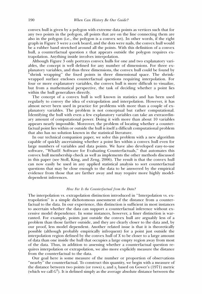
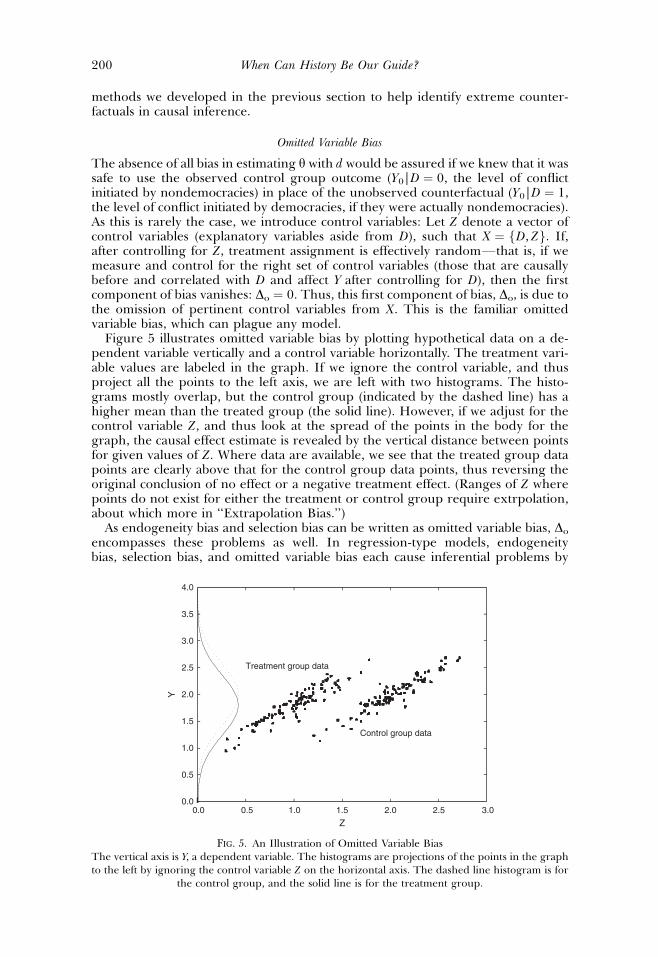
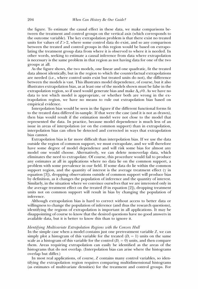
Figure 5 illustrates omitted variable bias by plotting hypothetical data on a de-pendent variable vertically and a control variable horizontally. The treatment vari-able values are labeled in the graph. If we ignore the control variable, and thusproject all the points to the left axis, we are left with two histograms. The histo-grams mostly overlap, but the control group (indicated by the dashed line) has ahigher mean than the treated group (the solid line). However, if we adjust for thecontrol variable Z, and thus look at the spread of the points in the body for thegraph, the causal effect estimate is revealed by the vertical distance between pointsfor given values of Z. Where data are available, we see that the treated group datapoints are clearly above that for the control group data points, thus reversing theoriginal conclusion of no effect or a negative treatment effect. (Ranges of Z wherepoints do not exist for either the treatment or control group require extrpolation,about which more in ‘‘Extrapolation Bias.’’)

As endogeneity bias and selection bias can be written as omitted variable bias, Do

encompasses these problems as well. In regression-type models, endogeneitybias, selection bias, and omitted variable bias each cause inferential problems by

0.0 0.5 1.0 1.5 2.0 2.5 3.00.0

0.5

1.0

1.5

2.0

2.5

3.0

3.5

4.0

Y

Z

Treatment group data

Control group data

FIG. 5. An Illustration of Omitted Variable BiasThe vertical axis is Y, a dependent variable. The histograms are projections of the points in the graphto the left by ignoring the control variable Z on the horizontal axis. The dashed line histogram is for

the control group, and the solid line is for the treatment group.


inducing a correlation between the explanatory variables and the error term. If wecontrol for the correct variables, then it is sometimes possible to eliminate theseproblems. In the omitted variable case, we can avoid the bias by including relevantvariables, such as common causes of D and Y. Similarly, we can avoid the biases dueto nonrandom selection if we control for the probability that each unit is selectedinto the sample, and we can eliminate endogeneity bias by including in the controlscovariates that eliminate the conditional relationship between X and the error term.

Post-Treatment Bias

Post-treatment bias is the second component of bias in our decomposition, Dp, andit deviates from zero when some of the control variables Z are at least in partconsequences of the key causal variable D. If Z includes these post-treatment vari-ables, then when the key causal variable D changes, the post-treatment variablesmay change too, and the plan to interpret the model as revealing the effect of thetreatment ‘‘holding other variables constant’’ becomes impossible.

As a simple example that illustrates the bias of controlling for post-treatmentvariables, suppose we are predicting the duration of an African dictatorship usingthe unemployment rate as the key explanatory variable. If we control for the ex-istence of a well-armed cabal inside the palace gates five minutes before a coupattempt is launched, our estimate of the effect of unemployment would be nearlyzero. The reason is that we are inappropriately controlling for the consequences ofour key causal variable, and for most of the effects of it, thus biasing the overalleffect. Yet, we certainly should control for a pre-treatment variable like the pres-ence of natural resources in the country, as it cannot be a consequence of un-employment but may be a common cause of both the explanatory and dependentvariables. Thus, causal models require separating out the pre- and post-treatmentvariables and controlling only for the pre-treatment, background characteristics.

Post-treatment variable bias may well be the largest overlooked component ofbias in estimating causal effects in political science (see King 1991; King, Keohane,and Verba 1994:173ff). It is well known in the statistical literature, but is assumedaway in most models and decompositions. This decision may be reasonable in otherfields, where the distinction between pre- and post-treatment variables is easier torecognize and avoid, but in political science and especially in comparative politicsand international relations, the problem is often severe. For example, is GDP aconsequence or cause of democracy? How about education levels? Fertility rates?Infant mortality? Trade levels? Are international institutions causes or consequen-ces of international cooperation? Many, or possibly even most, variables in theseliteratures are both causes and consequences of whatever is regarded as the treat-ment (or key causal) variable. As Lebow (2000:575) explains, ‘‘Scholars not infre-quently assume that one aspect of the past can be changed and everything else keptconstant, . . . [but these] ‘Surgical’ counterfactuals are no more realistic than surgicalair strikes.’’ This is especially easy to see in quantitative research when each of thevariables in an estimation takes its turn in different paragraphs of an article playingthe role of the ‘‘treatment.’’ However, only in rare statistical models, and only understringent assumptions, is it possible to estimate more than one causal effect from asingle model.

To avoid this component of bias, Dp, we need to ensure that we control for nopost-treatment variables, or that the distribution of our post-treatment variables donot vary with D. If this assumption holds, then Dp ¼ 0, so this component of bias in(5) vanishes.

In our field, unfortunately, we almost always need to consider both Do and Dp

together, and in many situations we cannot fix one without making the other worse.The same is not true in some other fields (which is perhaps the reason theDp component was ignored by Heckman et al. 1998), but it is rampant in ours.


Unfortunately, the news gets worse, as even the methodologist’s last resortFtry itboth ways, and if it does not make a difference, ignore the problemFdoes not workhere. Rosenbaum (1984) studies the situation where we run two analyses, oneincluding and one excluding the variables that are partly consequences and partlycauses of X. He shows that the true effect could be greater than these two or lessthan both. It is hard to emphasize sufficiently the seriousness of this problem andhow prevalent it is in comparative politics and international relations.

Although we have no general solution to this problem, we can offer one usefulway to avoid both Dp and Do in many practical applications. Aside from choosingbetter research designs in the first place, of course, our suggestion is to study whatwe call multiple-variable causal effects. If we cannot study the effects of democracycontrolling for GDP because higher GDP is in part a consequence of democracy, wemay be able to study the joint causal effect of a change from nondemocracy todemocracy and a simultaneous increase in GDP. This counterfactual is more real-istic, i.e., closer to the data, because it reflects changes that actually occur in theworld and does not require us to imagine holding variables constant that do notstay constant in nature. If we have specified a parametric model with both variables,we can study this question by simultaneously moving both GDP and democracy whileholding constant other variables at (say) their means. An alternative would be torecode the two variables into one on, as much as possible, a single dimension.

If this alternative formulation provides an interesting research question, then itcan be studied without bias due to Dp, as the joint causal effect will not be affected bypost-treatment bias. Moreover, the multiple-variable causal effect might also haveno omitted variable bias Do, as both variables would be part of the treatment andcould not be potential confounders. Of course, if this question is not of interest, andwe need to stick with the original question, then no easy solution exists at present.At that point, we should recognize that the counterfactual question being posed istoo unrealistic and too strained to provide a reasonable answer using the given datawith any statistical model. Either way, this is a serious problem that needs to movehigher on the agenda of political methodology.

Interpolation Bias

Even if we can be sure that no omitted variable or post-treatment biases exist, westill have to control for the observed pre-treatment variables properly. The tworemaining components of biasFinterpolation bias and extrapolation biasFbothhave to do with correctly identifying the necessary control variables but failing toadjust for them properly. Interpolation bias, or Di, results from adjusting incor-rectly for the correct control variables in regions of interpolation, and extrapolationbias results from adjusting for the correct controls where data are needed but donot exist. Interpolation bias is normally the less serious of the two as it is moreamenable to empirical testing.

Interpolation bias may exist in the simple difference in means estimator if themeasured control variables Z are related in any way to the treatment variable, that isif the multivariate density of Z for the treatment group differs from that for thecontrol group (within the region of interpolation). If in addition to these densitydifferences Z also affects the outcome variable, then interpolation bias will exist ifthe density differences in Z are not properly adjusted.

When using a parametric model to adjust for control variables, this component ofbias arises from controlling for Z with the wrong functional form. For example, inan application without post-treatment bias, with all control variables that couldcause bias identified, and where extrapolation is unnecessary, our estimator couldstill generate bias by choosing a linear model to adjust for controls if the data weregenerated from a quadratic. Fortunately, standard regression diagnostics are quiteuseful for checking model fit within the range of the data. Ultimately, whatever


method of adjustment is used, the two multivariate histograms of Z for the controland treatment groups need to be the same for interpolation bias to be eliminated.We provide further insight into interpolation bias during our discussion of ex-trapolation bias, to which we now turn.

Extrapolation Bias

The last component of bias, and the one most related to the central theme of thepaper, is extrapolation bias. This component is the second of the two that arise fromnot adjusting or improperly adjusting for identified control variables.

Extrapolation bias may arise when the support (or possible values) of the dis-tribution of Z for the treatment group differs from that of the control group. Thatis, there may be certain values of Z that some members of one group take on but nomembers of the other group possess. For example, we might observe no full dem-ocracies with GDP as low as in some of the autocracies, but we still somehow need tocontrol for GDP. Intuitively, these autocracies have no comparables in the data, sothey are not immediately useful for estimating causal effects. To make causal in-ferences in situations with nonoverlapping support, we must therefore either elim-inate the region outside of common supportFas is a standard practice in statisticsand medicineFor attempt to extrapolate to the needed data (e.g., autocracies withhigh GDP), such as by using a parametric modelFas is standard practice in politicalscience and most of the other social sciences. As we demonstrate in the previoussection, extrapolation in forecasting involves considerable model dependence. Thesame issue applies in causal inference, as we discuss here. Thus, unless we happento be in the extraordinary situation where a known theory or prior evidence makesit possible to narrow down the possible models to one, or where we happen to guessthe right model, we will be left with extrapolation bias, De6¼0.

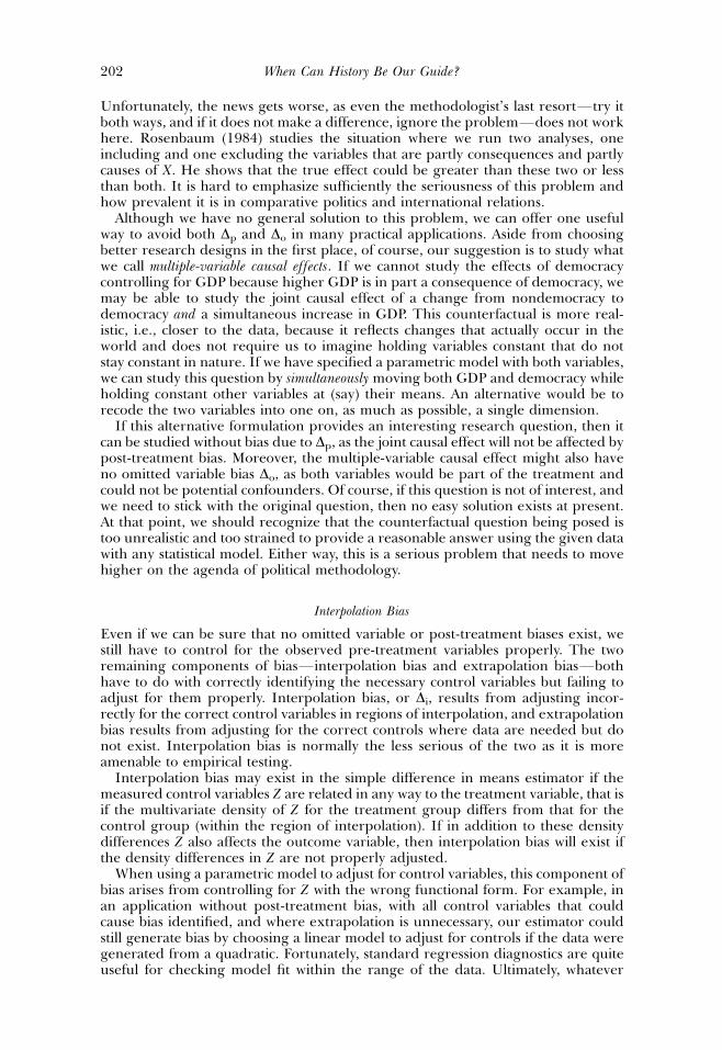
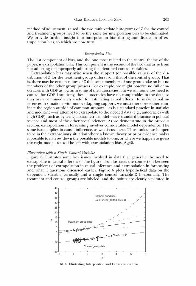
Illustration with a Single Control VariableFigure 6 illustrates some key issues involved in data that generate the need toextrapolate in causal inference. The figure also illustrates the connection betweenthe problems of extrapolation in causal inference and extrapolation in forecastingand what if questions discussed earlier. Figure 6 plots hypothetical data on thedependent variable vertically and a single control variable Z horizontally. Thetreatment and control groups are labeled, and the points are clearly separated in

Control group data

Treatment group data

0−20

−10

0

5

10

Y

15

20

25

30

35

40

45

1 2 3

Z4 5 6

Dashed: quadratic

Solid: linear (dotted: 95% CI)

FIG. 6. Illustrating Interpolation and Extrapolation Bias


the figure. To estimate the causal effect in these data, we make comparisons be-tween the treatment and control groups on the vertical axis (which corresponds tothe outcome variable). The key extrapolation problem is that there exist no treatedunits for values of Z42, where some control data do exist, and so any comparisonbetween the treated and control groups in this region would be based on extrapo-lating the treatment group data from where it is observed to where it is needed. Inother words, seeking to estimate a causal inference from data where extrapolationis necessary is the same problem in that region as not having data for one of the twogroups at all.

As the figure shows, the two models, one linear and one quadratic, fit the treateddata almost identically, but in the region to which the counterfactual extrapolationsare needed (i.e., where control units exist but treated units do not), the differencebetween the models is vast. This illustrates model dependence, of course, but it alsoillustrates extrapolation bias, as at least one of the models shown must be false in theextrapolation region, so if used would generate bias and make De6¼0. As we have nodata to test which model is appropriate, or whether both are wrong in the ex-trapolation region, we have no means to rule out extrapolation bias based onempirical evidence.

Interpolation bias would be seen in the figure if the different functional forms fitto the treated data differed in-sample. If that were the case (and it is not as drawn),then bias would result if the estimation model were not close to the model thatrepresented the data. In practice, because model dependence is much less of anissue in areas of interpolation (or on the common support) than in extrapolation,interpolation bias can often be detected and corrected in ways that extrapolationbias cannot.

Extrapolation bias is far more difficult than interpolation bias. If we use the dataoutside the region of common support, we must extrapolate, and we will thereforehave some degree of model dependence and will risk some bias for almost anymodel one would choose. Alternatively, we can delete nonoverlap data, whicheliminates the need to extrapolate. Of course, this procedure would fail to produceany estimates at all in applications where no data lie on the common support, aproblem with some prevalence in our field. If some data do lie within the commonsupport region, and the quantity of interest is the average treatment effect (g inequation [3]), dropping observations outside of common support will produce biasby definition, as it changes the population of inference and the quantity of interest.Similarly, in the situation where we convince ourselves that we are interested only inthe average treatment effect on the treated (y in equation [2]), dropping treatmentunits not on common support will result in bias by changing the population ofinference.

Although extrapolation bias is hard to correct without access to better data orwillingness to change the population of inference (and thus the research questions),identifying the regions of extrapolation is important in all applications. It may bedisappointing of course to know that the desired questions have no good answers inavailable data, but it is better to know this than to ignore it.

Identifying Multivariate Extrapolation Regions with the Convex HullIn the simple case when a model contains just one pretreatment variable Z, we cansimply plot a histogram of this variable for the treated (Di ¼ 1) units on the samescale as a histogram of this variable for the control (Di ¼ 0) units, and then comparethem. Areas requiring extrapolation can easily be identified as the areas of thehistograms that do not overlap. (Interpolation bias can arise where the histogramsoverlap but differ.)

In most real applications, of course, Z contains many control variables, so iden-tifying the extrapolation region requires comparing multidimensional histograms(as estimates of multivariate densities) for the treatment and control groups. For


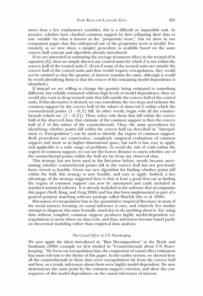
more than a few explanatory variables, this is a difficult or impossible task. Inpractice, scholars have checked common support by first collapsing their data toone variable via what is known as the ‘‘propensity score,’’ but we show in ourcompanion paper that this widespread use of the propensity score is invalid. For-tunately, as we now show, a simpler procedure is available based on the sameconvex hull concept and algorithm already introduced.

If we are interested in estimating the average treatment effect on the treated (y inequation [2]), then we simply discard any control units for which Z is not within theconvex hull of the treated units Z. (Even if some of the treated units are outside theconvex hull of the control units and thus would require extrapolation, they wouldnot be omitted so that the quantity of interest remains the same, although it wouldbe worth identifying them so that the source of the remaining model dependence isidentified.)

If instead we are willing to change the quantity being estimated to somethingdifferent, but reliably estimated without high levels of model dependence, then wewould also want to drop treated units that fall outside the convex hull of the controlunits. If this alternative is desired, we can consolidate the two steps and estimate thecommon support by the convex hull of the subset of observed Z within which thecounterfactual points f1� D, Zg fall. In other words, begin with all the counter-factuals (which are f1� D, Zg). Then, select only those that fall within the convexhull of the observed data. Our estimate of the common support is then the convexhull of Z of this subset of the counterfactuals. Thus, the same procedures foridentifying whether points fall within the convex hull (as described in ‘‘Interpol-ation vs. Extrapolation’’) can be used to identify the region of common support.Both procedures are conservative, completely empirical evaluations of commonsupport and more so in higher-dimensional space, but each is fast, easy to apply,and applicable to a wide range of problems. To avoid the risk of voids within theregion of common support, we can use the Gower distance to assess whether any ofthe counterfactual points within the hull are far from any observed data.

This strategy has not been used in the literature before, mostly because ascer-taining whether counterfactual points fall in the convex hull has not previouslybeen viewed as feasible. Given our new algorithm for finding whether points fallwithin the hull, this strategy is now feasible, and easy to apply. Indeed, a keyadvantage of the strategy suggested here is that at least a good first cut at findingthe region of common support can now be automated and easily included instandard statistical software. It is already included in the software that accompaniesthis paper (Stoll, King, and Zeng 2006) and has also been implemented as part of ageneral purpose matching software package called MatchIt (Ho et al. 2006).

Discussion of extrapolation bias in the quantitative empirical literature in most ofthe social sciences focusing on causal inference is rare, and relatively few studiesattempt to diagnose this issue formally, much less to do anything about it. Yet, usingdata without complete common support produces highly model-dependent ex-trapolations to areas where no data exist, and thus, inferences become based partlyon theoretical modeling rather than empirical data analyses.

The Causal Effect of UN Peacekeeping

We now apply the ideas introduced in ‘‘Bias Decomposition’’ to the Doyle andSambanis (2000) example we first studied in ‘‘Counterfactuals about UN Peace-keeping.’’ We focus on extrapolation bias, the component of causal effect estimationbias most relevant to the theme of this paper. In the earlier section, we showed howall the counterfactuals in these data were extrapolations far from the convex hulland how, as a result, inferences about them were highly model-dependent. We nowdemonstrate the same point by the common support criterion, and show the con-sequence of this model dependence on the causal inferences of interest.


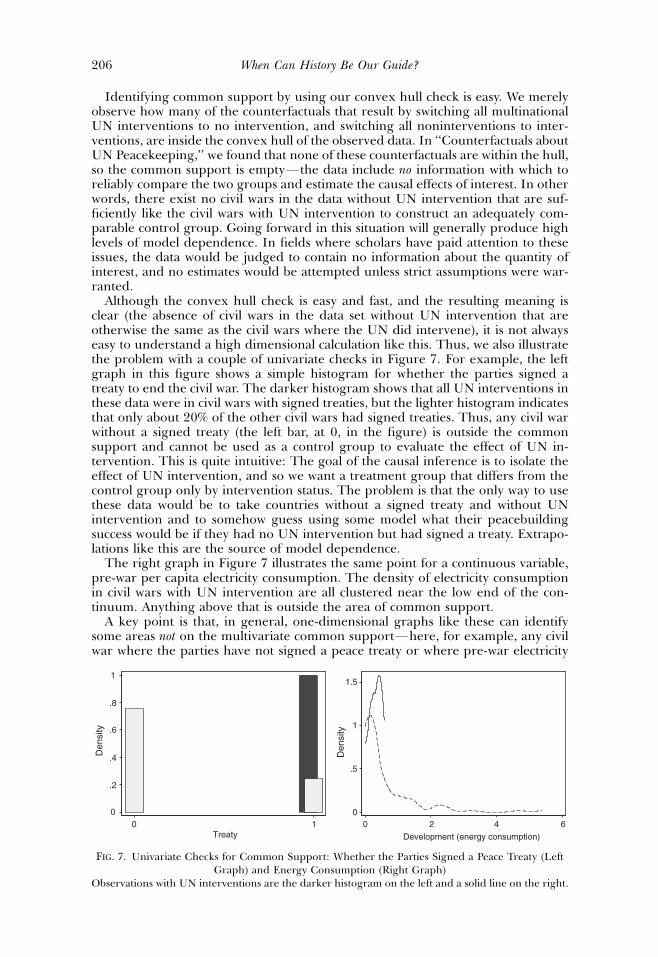
Identifying common support by using our convex hull check is easy. We merelyobserve how many of the counterfactuals that result by switching all multinationalUN interventions to no intervention, and switching all noninterventions to inter-ventions, are inside the convex hull of the observed data. In ‘‘Counterfactuals aboutUN Peacekeeping,’’ we found that none of these counterfactuals are within the hull,so the common support is emptyFthe data include no information with which toreliably compare the two groups and estimate the causal effects of interest. In otherwords, there exist no civil wars in the data without UN intervention that are suf-ficiently like the civil wars with UN intervention to construct an adequately com-parable control group. Going forward in this situation will generally produce highlevels of model dependence. In fields where scholars have paid attention to theseissues, the data would be judged to contain no information about the quantity ofinterest, and no estimates would be attempted unless strict assumptions were war-ranted.

Although the convex hull check is easy and fast, and the resulting meaning isclear (the absence of civil wars in the data set without UN intervention that areotherwise the same as the civil wars where the UN did intervene), it is not alwayseasy to understand a high dimensional calculation like this. Thus, we also illustratethe problem with a couple of univariate checks in Figure 7. For example, the leftgraph in this figure shows a simple histogram for whether the parties signed atreaty to end the civil war. The darker histogram shows that all UN interventions inthese data were in civil wars with signed treaties, but the lighter histogram indicatesthat only about 20% of the other civil wars had signed treaties. Thus, any civil warwithout a signed treaty (the left bar, at 0, in the figure) is outside the commonsupport and cannot be used as a control group to evaluate the effect of UN in-tervention. This is quite intuitive: The goal of the causal inference is to isolate theeffect of UN intervention, and so we want a treatment group that differs from thecontrol group only by intervention status. The problem is that the only way to usethese data would be to take countries without a signed treaty and without UNintervention and to somehow guess using some model what their peacebuildingsuccess would be if they had no UN intervention but had signed a treaty. Extrapo-lations like this are the source of model dependence.

The right graph in Figure 7 illustrates the same point for a continuous variable,pre-war per capita electricity consumption. The density of electricity consumptionin civil wars with UN intervention are all clustered near the low end of the con-tinuum. Anything above that is outside the area of common support.

A key point is that, in general, one-dimensional graphs like these can identifysome areas not on the multivariate common supportFhere, for example, any civilwar where the parties have not signed a peace treaty or where pre-war electricity

0

.2

.4

.6

.8

1

Den

sity

0 1Treaty

0

.5

1

1.5

Den

sity

0 2 4 6

Development (energy consumption)

FIG. 7. Univariate Checks for Common Support: Whether the Parties Signed a Peace Treaty (LeftGraph) and Energy Consumption (Right Graph)

Observations with UN interventions are the darker histogram on the left and a solid line on the right.


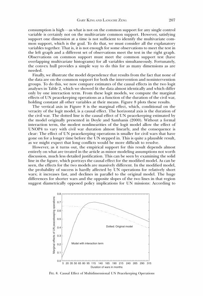
consumption is highFas what is not on the common support for any single controlvariable is certainly not on the multivariate common support. However, satisfyingsupport one dimension at a time is not sufficient to identify the multivariate com-mon support, which is the goal. To do that, we must consider all the explanatoryvariables together. That is, it is not enough for some observations to meet the test inthe left graph and a different set of observations meet the test in the right graph.Observations on common support must meet the common support test (haveoverlapping multivariate histograms) for all variables simultaneously. Fortunately,the convex hull provides a simple way to do this for as many dimensions as areneeded.

Finally, we illustrate the model dependence that results from the fact that none ofthe data are on the common support for both the intervention and noninterventiongroups. To do this, we now compare estimates of the causal effects in the two logitanalyses in Table 2, which we showed fit the data almost identically and which differonly by one interaction term. From these logit models, we compute the marginaleffects of UN peacekeeping operations as a function of the duration of the civil war,holding constant all other variables at their means. Figure 8 plots these results.

The vertical axis in Figure 8 is the marginal effect, which, conditional on theveracity of the logit model, is a causal effect. The horizontal axis is the duration ofthe civil war. The dotted line is the causal effect of UN peacekeeping estimated bythe model originally presented in Doyle and Sambanis (2000). Without a formalinteraction term, the modest nonlinearities of the logit model allow the effect ofUNOP4 to vary with civil war duration almost linearly, and the consequence isclear: The effect of UN peacekeeping operations is smaller for civil wars that havegone on for a longer time before the UN stepped in. This is quite a plausible result,as we might expect that long conflicts would be more difficult to resolve.

However, as it turns out, the empirical support for this result depends almostentirely on what are treated in the article as minor modeling assumptions not worthdiscussion, much less detailed justification. This can be seen by examining the solidline in the figure, which portrays the causal effect for the modified model. As can beseen, the effects for the two models are massively different. In the modified model,the probability of success is hardly affected by UN operations for relatively shortwars; it increases fast, and declines in parallel to the original model. The hugedifferences for shorter wars and the opposite slopes of the two lines in that regionsuggest diametrically opposed policy implications for UN missions: According to

Duration of wars in months

Model with interaction term

Dotted: Original model

5 20 35 50 65 80 95 115 140 165 190 215 240 265 290 315

Mar

gina

l effe

cts

of U

N p

eace

keep

ing

oper

atio

ns

0.0

0.1

0.2

0.3

0.4

0.5

0.6

0.7

0.8

FIG. 8. Causal Effect of Multidimensional UN Peacekeeping Operations


one model, wars with the shortest duration should receive the most attention fromthe UN, as that is where the model indicates that the UN can have its biggest effect;according to the other model, the same civil wars should receive the least attentionfrom the UN. (Confidence intervals confirm that inferences from the two modelsusing more than point estimates also differ with dramatically different policy im-plications.) Although the two models gave nearly identical fit to the factual data, thecounterfactuals are far enough from the observed data to make conclusions highlysensitive to modeling assumptions. To be clear, no theory offered in Doyle andSambanis (2000) or the literature would rule out one of the two models, and thedata do not enable us to choose one either. We also do not prefer the modifiedmodel over the original and introducing the modification only as an illustration ofthe extreme model dependence that can result from using data outside of commonsupport that requires extrapolation.

Concluding Remarks

Even far-out questions with answers that are highly model-dependent may still beimportant enough to warrant further study. The following are a few examples:What would be the future of military conflict if globalization led to a world withoutnation states? How bad would the devastation be from a third world war? If a newvirulent infectious disease that is ten times as bad as AIDS strikes the developedworld and lasts longer than the AIDS crisis, would current international institutionssurvive? Scholars can and certainly still should ask questions like these, but wewould be better served if we knew whether and to what degree our answers to themare based on empirical evidence rather than model assumptions. Sometimes, withthe data at hand, no statistical model can give valid answers, and we must rely ontheory or new data collection efforts. The techniques offered in this paper may beuseful in ascertaining the degree to which this is the case. In this regard, it may beuseful for empirical researchers to report these or other statistics, or to at leastaddress the problem in some way when they evaluate their counterfactuals.

We have used the methods discussed here to evaluate counterfactuals in the largearea of research devoted to assessing the effects of democracy. We found thatquestions about democracy with empirical answers that are not highly model-de-pendent are a subsetFsometimes a small subsetFof those that have been asked.Usually scholars combine data on all available democracies and autocracies to makepredictions, ask ‘‘what if ’’ questions, or estimate causal effects. Unfortunately, manyof the explicit or implied questions have no available control groups or otherwisecannot be estimated without making assumptions that even the authors wouldprobably be unwilling to defend. We might like to know what would happen if Iraqbecame a full democracy, for example, but history cannot be our guide as almost noevidence exists in our data with which to evaluate such a question. Although havingsmall numbers of cases will often make finding a proper control group harder, inthis example, having access to time-series-cross-sectional data sets with thousands ofobservations does not change this basic fact and will not make inferences like theseany more secure. In fact, these data sets must be analyzed with more care than hasbeen common since, as it turns out, they do not include much evidence on manyotherwise interesting counterfactuals. Asking questions about the effects of changesin democracy averaged over all countriesFthe predominant approach taken in theliteratureFalmost always implies questions without adequate empirical evidence toanswer. Statistical analyses in data sets like these should change: scholars could seekdifferent types of evidence, develop better theory, or narrow their inferentialtarget to a subset of countries and counterfactuals that have empirical support intheir data.

Suppose we read about a model that fits the data exceedingly well, has abig likelihood ratio or F statistics, narrow confidence intervals, significance on all


coefficients, large causal effect estimates, predictions with path-breaking policy im-plications, and fascinating answers to a range of ‘‘what if ’’ questions. With statisticalreporting standards now commonly used in political science, essentially all suchmodels would be published and taken seriously by readers. A subset of these,however, would involve inferences that are so model-dependent as to be nearlyunrelated to the data at hand, based more on the authors’ hypotheses and con-venient model assumptions than their data. The main message of this article is thatassessing model dependence of counterfactual questions needs to be a routine andexpected part of statistical reporting for anyone making predictions, asking ‘‘whatif ’’ questions, and estimating causal effectsFwhich together encompasses the goalsof a large fraction of empirical work in the discipline.

References

DOYLE, MICHAEL W., AND NICHOLAS SAMBANIS. (2000) International Peacebuilding. American PoliticalScience Review 94(4):779–801.

DOZOIS, GARDNER, AND STANLEY SCHMIDT, EDS. (1998) Roads not Taken: Tales of Alternative History. NewYork: Del Rey.

ESTY, DANIEL C., JACK GOLDSTONE, TED ROBERT GURR, BARBARA HARFF, PAMELA T. SURKO, ALAN N.UNGER, AND ROBERT S. CHEN. (1998) The State Failure Task Force Report: Phase II Findings. McLean:Science Applications International Corporation.

FEARON, JAMES D. (1991) Counterfactuals and Hypothesis Testing in Political Science. World Politics43(2):169–195.

GELMAN, ANDREW, AND GARY KING. (1994) Party Competition and Media Messages in U.S. PresidentialElection Campaigns. In The Parties Respond: Changes in the American Party System, edited by SandyL. Maisel. Boulder: Westview Press. Available at http://gking.harvard.edu/files/abs/partycomp-abs.shtml.

GOWER, J. C. (1971) A General Coefficient of Similarity and Some of its Properties. Biometrics 27:857–872.

HASTIE, TREVOR, R. TIBSHIRANI, AND J. FRIEDMAN. (2001) The Elements of Statistical Learning. New York:Springer Verlag.

HECKMAN, JAMES J., HIDEHIKO ICHIMURA, JEFFREY SMITH, AND PETRA TODD. (1998) CharacterizingSelection Bias Using Experimental Data. Econometrika 66(5):1017–1098.

HO, DANIEL, KOSUKE IMAI, GARY KING, AND ELIZABETH STUART. (2007) Matching as NonparametricPreprocessing for Parametric Causal Inference. Political Analysis (forthcoming). Available athttp://gking.harvard.edu/files/abs/matchp-abs.shtml.

HOLLAND, PAUL W. (1986) Statistics and Causal Inference. Journal of the American Statistical Association81:945–960.

KING, GARY. (1991) Truth Is Stranger than Prediction, More Questionable Than Causal Inference.American Journal of Political Science 35(4):1047–1053. Available at http://gking.harvard.edu/files/abs/truth-abs.shtml.

KING, GARY, ROBERT O. KEOHANE, AND SIDNEY VERBA. (1994) Designing Social Inquiry: Scientific Inferencein Qualitative Research. Princeton: Princeton University Press.

KING, GARY, MICHAEL TOMZ, AND JASON WITTENBERG. (2000) Making the Most of Statistical Analyses:Improving Interpretation and Presentation. American Journal of Political Science 44(2):341–355.Available at http://gking.harvard.edu/files/abs/making-abs.shtml.

KING, GARY, AND LANGCHE ZENG. (2002) Improving Forecasts of State Failure. World Politics 53(4):623–658. Available at http://gking.harvard.edu/files/abs/civil-abs.shtml.

KING, GARY, AND LANGCHE ZENG. (2006a) The Dangers of Extreme Counterfactuals. Political Analysis14(2):131–159. Available at http://gking.harvard.edu/files/abs/counterft-abs.shtml.

KING, GARY, AND LANGCHE ZENG. (2006b) ‘‘Replication Data Set for ‘When Can History Be Our Guide?The Pitfalls of Counterfactual Inference.’ ’’ Available at http://id.thedata.org/hdl%3A1902.1%2FDXRXCFAWPK hdl:1902.1/DXRXCFAWPK UNF:3:DaYlT6QSX9r0D50ye+tXpA== MurrayResearch Archive [distributor(DDI)].

KUO, YEN-HONG. (2001) ‘‘Extrapolation of Association Between Two Variables in Four GeneralMedical Journals.’’ Fourth International Congress on Peer Review in Biomedical Publication,September.

KVART, IGAL. (1986) A Theory of Counterfactuals. Indianapolis: Hackett Publishing Company.LEBOW, RICHARD NED. (2000) What’s so Different About a Counterfactual? World Politics 52:550–585.


LEWIS, DAVID K. (1973) Counterfactuals. Cambridge: Harvard University Press.MURPHY, GEORGE G. S. (1969) On Counterfactual Propositions. History and Theory 9:14–38.PEARL, JUDEA. (2000) Causality: Models, Reasoning, and Inference, Cambridge University Press.ROBINS, JAMES M. (1999a) Marginal Structural Models Versus Structural Nested Models as Tools for

Causal Inference. In Statistical Models in Epidemiology: The Environment and Clinical Trials, Vol. 116.edited by M. E. Halloran and D. Berry. New York: Springer-Verlag.

ROBINS, JAMES M. (1999b) Association, Causation, and Marginal Structural Models. Synthese 121:151–179.

ROSENBAUM, PAUL. (1984) The Consequences of Adjusting for a Concomitant Variable That Has BeenAffected by the Treatment. Journal of the Royal Statistical Society, A 147(5):656–666.

RUBIN, DONALD B. (1974) Estimating Causal Effects of Treatments in Randomized and Nonrandom-ized Studies. Journal of Educational Psychology 6:688–701.

STOLL, HEATHER, GARY KING, AND LANGCHE ZENG. (2006) WhatIf: Software for Evaluating Counter-factuals. Journal of Statistical Software 15(4). Available at http://gking.harvard.edu/whatif/.

TALLY, STEVE. (2000) Almost America: From the Colonists to Clinton, A ‘‘What If ’’ History of the U.S. NewYork: Quill.

TETLOCK, PHILIP E. (1999) Theory-Driven Reasoning About Plausible Pasts and Probable Futures inWorld Politics: Are We Prisoners of Our Preconceptions. American Journal of Political Science43(2):335–366.

TETLOCK, PHILIP E., AND A. BELKIN, EDS. (1996) Counterfactual Thought Experiments in World Politics.Princeton: Princeton University Press.

TETLOCK, PHILIP E., AND RICHARD NED LEBOW. (2001) Poking Counterfactual Holes in Covering Laws:Cognitive Styles and Historical Reasoning. American Political Science Review 95(4):829–843.

TETLOCK, PHILIP E., NED R. LEBOW, AND G. PARKER, EDS. (2000) Unmaking the West: CounterfactualExplorations of Alternative Histories. New York: Columbia University Press.

THORSON, STUART J., AND DONALD A. SYLVAN. 1982 Counterfactuals and the Cuban Missile Crisis.International Studies Quarterly 26(4):539–571.


when can history be our guide? the pitfalls of counterfactual inference

Documents