what’s inside - invensysiom.invensys.com/en/pdflibrary/whitepaper_loadsheddingand... · load...

Foxboro SCADA Systems Load Shedding and Electrical Monitoring Control Systems Design in Industrial Process Plants

Author: Mark Grant

What’s Inside

1. Load Shedding System (LSS)

2. Elecsolve Power Modeling

3. Event Disturbance Record System

4. References

Load Shedding System

1. Load Shedding System (LSS) The load shedding or disconnection of non-essential loads is a vital strategy to avoid a major electric power system breakdown during a disturbance, such as with the tripping of a generator during which case the load demand becomes greater than the generation could supply. The Load Shedding System (LSS) is provided in this project and it becomes an important part in the Generation Management System and is integrated with the power generation control strategy in automatic generation and load operations. Primary load shedding may be initiated consequently to one of the following events:

Generator Trip Tripping of Turbine Generators Tripping of Generator Circuit Breakers Overload condition persists (typically 20-30 seconds)

In addition to the above tripping events, LSS can also be triggered by absolute frequency trigger points, and by df/dt (rate of change of frequency,) as calculated by logic and transducers, which act as a backup function to the above triggering conditions. In these situations, the power supply available may not be able to support the existing plant load. To prevent overloading of the remaining generators in the system, which may lead to the total collapse of the system, it is important to reduce plant load to less than the available generation capacity and thereby avoid total disruption to plant operation. Non-essential feeder loads supplying various end user substations, will be tripped with predefined sequences in order to maintain the nominal power system frequency and stability of electrical network. (Note that the term “non essential” is relative to the power generation assets, and obviously is not to be construed as non essential to the end user. In order to save the network however, something must be sacrificed.) In primary load shedding logic, under frequency load shedding will be activated when the frequency decays in a pre-defined rate irrespective of above mentioned events. The df/dt setting is tunable at site.

1.1 Load Shedding System Functionality Overview The Load Shedding is initiated based one of the following events:

A device trip/open event that causes the demand to exceed the generation capability – Fast Load Shedding

Under-frequency conditions – Slow Load Shedding When managing on-site generation or power from the grid, loads will be tripped with predefined sequences in order to maintain the nominal power system frequency and stability of electrical network.

2


1.1.1 Fast Load Shedding The Fast Load Shedding is activated in less than 100 milliseconds in order to prevent damage to motors and turbines caused by frequency anomalies. Other causes of fast load shedding requirements are from:

Generator Trip Tripping of any Generators Tripping of Generator Circuit Breakers

1.1.2 Slow Load Shedding

Slow load shedding monitors overload and frequency events. Slow load shedding is activated as follows:

The frequency falls below 58.5Hz The frequency decays faster than a pre-defined rate. The df/dt (change in frequency per time) setting is

tunable at site 1.2 Load Shedding Algorithm Every generator in the system has a maximum capacity for its particular operating circumstance. The plant generation controls will utilize all available capacity in order to maintain frequency at 60Hz. The system normally will have excess capacity and the generators will not be fully loaded. However, in the event that plant load exceeds the capacity of the generators, then the system will become out of balance and frequency will decay. Load shedding systems also continuously monitor the excess capacity of the generators or incoming feeders and use this calculation as the main determinant of how much load to shed. The goal of the load shedding system is to keep Power Margin (PM) positive.

Power Margin = (Sum of Generator Capacity) – (Total Plant Load)

1.2.1 Slow Load Shedding For on-site power generation the loss of a generator contributes to the capacity calculation. If the Power Margin returns a negative value, then a load shed trigger is activated. Generation control systems will attempt to load the remaining generators to their maximums, but cannot achieve 60Hz which will drive the load shedding process. 1.2.2 Plant Capacity Overload When plant load has increased above the Generator Capacity and the Power Margin calculation has returned a negative value. Transient overloads must be considered such as a large load starting up. In these cases an adjustable time delay should be considered and inserted into the trigger logic to allow the transient to pass, and avoid unnecessary load shedding. Of course, if the Power Margin is still negative after the time delay has elapsed, then Load Shedding is triggered.

3


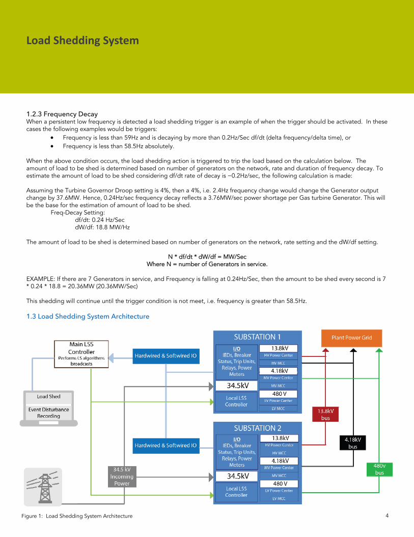
1.2.3 Frequency Decay When a persistent low frequency is detected a load shedding trigger is an example of when the trigger should be activated. In these cases the following examples would be triggers:

Frequency is less than 59Hz and is decaying by more than 0.2Hz/Sec df/dt (delta frequency/delta time), or Frequency is less than 58.5Hz absolutely.

When the above condition occurs, the load shedding action is triggered to trip the load based on the calculation below. The amount of load to be shed is determined based on number of generators on the network, rate and duration of frequency decay. To estimate the amount of load to be shed considering df/dt rate of decay is −0.2Hz/sec, the following calculation is made: Assuming the Turbine Governor Droop setting is 4%, then a 4%, i.e. 2.4Hz frequency change would change the Generator output change by 37.6MW. Hence, 0.24Hz/sec frequency decay reflects a 3.76MW/sec power shortage per Gas turbine Generator. This will be the base for the estimation of amount of load to be shed.

Freq-Decay Setting: df/dt: 0.24 Hz/Sec dW/df: 18.8 MW/Hz

The amount of load to be shed is determined based on number of generators on the network, rate setting and the dW/df setting.

N * df/dt * dW/df = MW/Sec

Where N = number of Generators in service. EXAMPLE: If there are 7 Generators in service, and Frequency is falling at 0.24Hz/Sec, then the amount to be shed every second is 7 * 0.24 * 18.8 = 20.36MW (20.36MW/Sec) This shedding will continue until the trigger condition is not meet, i.e. frequency is greater than 58.5Hz. 1.3 Load Shedding System Architecture

4 Figure 1: Load Shedding System Architecture


1.3.1 Frequency Decay The Load Shedding System consists of the following modules:

LSS Master Station – It provides Load Shedding System configuration, setting, user interface and functional controls. This is contained in the standard Foxboro SCADA Operator Interface powered by Wonderware.

Main LSS Controller –It executes the main load shedding command in the Foxboro SCD5200 RTU. In some cases the Main LSS Controller is in a redundant configuration and might be located in one of the substations. In this case, the Main LSS Controller would send load shed sequences to local substations if the local LSS Controller goes down.

Local LSS Controller –It controls load feeders and other devices in the substation. The SCD5200 RTU is installed in each of the feeder substations.

1.4 Load Shed System Module Design 1.4.1 Master Station The LSS Master station is the center of the LSS for data processing and controls. It provides the following functionalities to the Load Shed System:

Real-time data collection from SCADA/GMS, LSS Main Controller and Local Controllers Data process and periodical Calculations (once every 5-10 seconds) Downloading of LSS Logical Schema and settings to Main Controller Monitoring of the LSS program process Operator manual control of LSS System Configuration User Graphical Interface (HMI) Historian Alarms

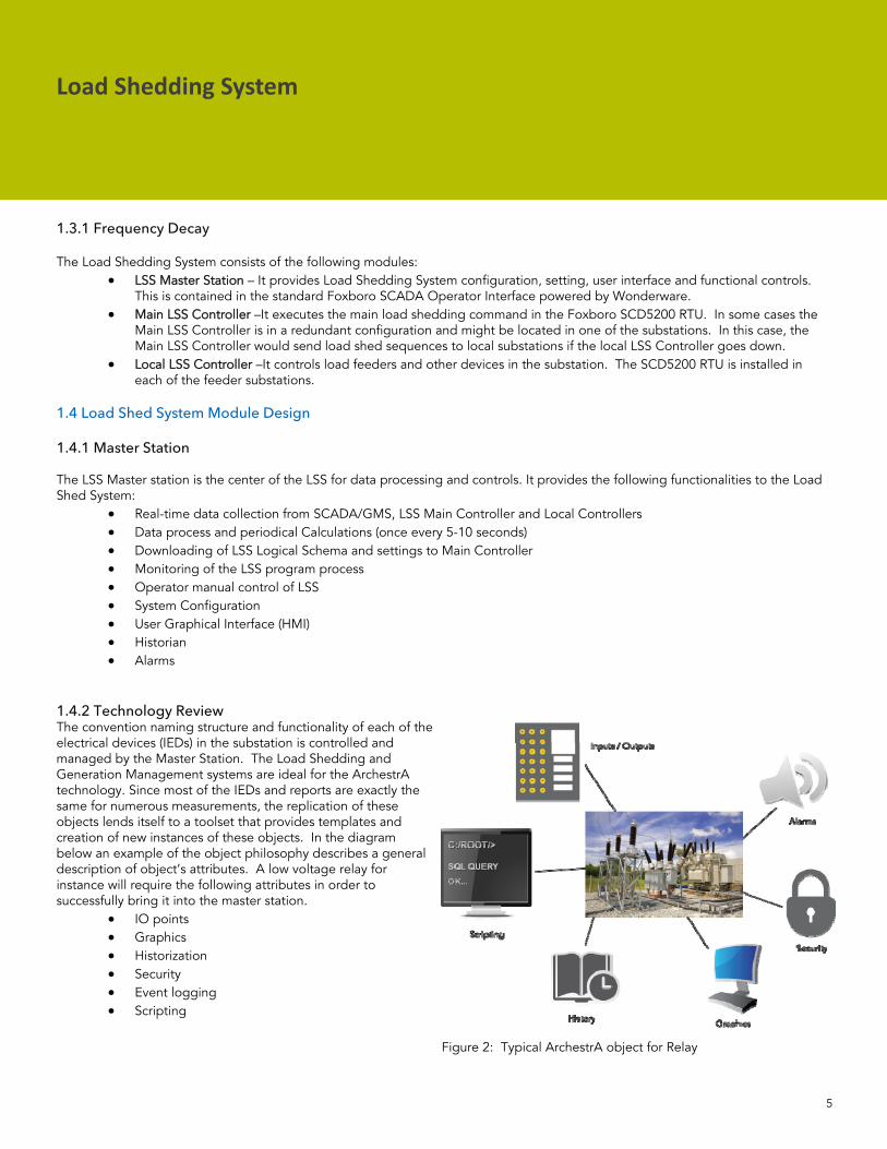
1.4.2 Technology Review The convention naming structure and functionality of each of the electrical devices (IEDs) in the substation is controlled and managed by the Master Station. The Load Shedding and Generation Management systems are ideal for the ArchestrA technology. Since most of the IEDs and reports are exactly the same for numerous measurements, the replication of these objects lends itself to a toolset that provides templates and creation of new instances of these objects. In the diagram below an example of the object philosophy describes a general description of object’s attributes. A low voltage relay for instance will require the following attributes in order to successfully bring it into the master station.

IO points Graphics Historization Security Event logging Scripting

5

Figure 2: Typical ArchestrA object for Relay


The functionalities of the Master Station are achieved through the following components:

The LSS Master Station is integrated into the Invensys Generation Management System on the ArchestrA Application Platform environment

The main LSS logic runs within the ArchestrA objects on a dedicated Application Engine The Configuration of the LSS is provided by the Foxboro IDE (Integrated Development Environment) The LSS History data functions are provided by Foxboro SCADA/GMS Historian The LSS Alarm functions are provided by Foxboro SCADA/GMS Alarm System Data communication to Main controller and Local controllers is implemented via DNP protocol on Ethernet

1.4.3 Main Load Shedding Controller The main load shedding controller is typically housed in one of the substations and it is used as the primary load shedding controller where the algorithms are loaded and executed. During a load shedding event the main controller will act as a broadcaster of messages to local substations where the load shedding logic is executed per pre-defined truth tables. The execution logic is then pushed to the local load shedding controller which is responsible for the actual execution of activities. The main load shedding controller provides the following functionalities:

Collects real-time data Executes load shedding logic Issues load shedding trip commands to Local Controller Issues direct DO command to Circuit Breakers as needed Sends load shedding data to master SCADA station

The LSS load shedding logic execution details are as follows:

The load shedding detection algorithm runs every 10 milliseconds. When the load shed condition is detected, a pre-determined matrix of truth tables is searched for the correct load shed sequence to follow.

Once the load shed sequence has been determined (within 10 msec of the event), a dedicated message will be broadcast to all of the LSS Local Controllers in the other substations using a dedicated fiber network. Using a dedicated fiber network is critical to maintain less than 100 millisecond response from event recognition to substation actions such as opening breakers, shutting down motors, etc… Each local controller shall receive an index which is used locally in each local controller to determine which relays to operate. In order to maintain a level of redundancy good, engineering practice defines that each local load shed controller in each substation shall run the algorithm redundantly. It, therefore, provides the local trip signals to the local breakers according to the pre-determined load shed sequence.

The functionalities of the main controller are achieved through the following components:

The LSS main controller is integrated into the Foxboro SCD5200 RTU.

The LSS logic is implemented using SCD5200 calculation function

Data communication to master station and local controllers is implemented via DNP protocol on Ethernet

6

Foxboro SCD5200

1.4.4 Local SCD5200 Controller The LSS local controller provides the following functionalities:

Collects and processes real-time data Issues direct DO command to circuit breakers Sends load shed system data to master station and main controllers

The functionalities of the local controller are achieved through the following components:

The LSS local controller is integrated into the Foxboro SCD5200 Station Control Device. The LSS logic is implemented using SCD5200 calculation function Data communication to Master Station and Main Controller is implemented via DNP protocol on Ethernet Acts as a redundant controller to sense network failure and take control of scanning functions to the RS485 link.

1.5 Load Shedding System HMI Displays The LSS user interface is provided through the Wonderware InTouch for Foxboro SCADA. Typical user graphic windows dedicated to load shedding include:

Load Shedding Overview Display Load shed overview display depicts the running status of the primary load shedding logic, frequency

measured on each bus, frequency decay (df/dt), load on each generator, generator maximum capacity of each generator, power margin, and the spinning reserve available.

The engineer with an authorized system administrative level can disable/enable the primary load shedding system execution through the display.

Master Load Shed List Display A master load shed list graphic displays all details of the static data (tag number, tag description, substation

number, switchboard number and train number), sequence number, and priority number along with the updated “nominal” values for sheddable load.

A priority set of integers is typically used to change the shedding sequence and the sequence change would be shown on the display.

Active Load Shed List Display

The active load shed list display provides the operator with the list of selected loads (sorted based on priority) to be shed during the actual load shedding sequence.

Alarms When the Power Margin falls below a pre-defined level a critical alarm is generated to warn the operator of

approaching overload conditions. When any of the triggering events occurs, and load shedding is enabled, an alarm is generated to warn the

operator that load shedding is initiated.


7


1.6 Load Shedding System Calculations and Considerations 1.6.1 Load and Generation Calculation In order for the load shedding application to be continually accurate the calculations must be dynamic. The load shedding application must perform calculations on the system load. First the total operating load must be determined from the sum of all the feeder loads. The loads include:

All feeders at 34.5kV All main medium voltage feeders to final or intermediate substations All individual electrical loads with power consumption above 2MVA

The other calculation that must be made is system generation. The load shedding application must identify the available load. The load shedding application calculates the system generation with the following dynamic measurements:

The total generation capacity – generators that are online The total spinning reserve MW that equals Total Capacity – Total actual generation MW Power Margin that equals Total Capacity – Total Load

If steam generators are involved tunable factors are applied due to slower response time and steam loading consideration. This is factored into the capacity calculation for the steam turbines to reflect the actual contribution of these generators to the spinning reserve during load shedding. The Load shedding system also calculates frequency deviation and rate of change and blocks of sheddable loads that need to be shed at various low frequency levels. 1.7 Load Shedding Logic Execution The load shedding logic is executed by using a combination of discrete calculations and sequence blocks. The logic consists of three basic steps (a) pre-calculation; (b) triggering condition; and (c) load tripping. Step 1: Pre-calculation The pre-calculation of load to be tripped, compares (in ascending priority order) the MW value of the loads in the priority list, starting from lowest priority. The loads of the next higher priority are added to this until the cumulative total is greater than the required value. This sorted list constitutes the amount of load to be tripped. Step 2: Triggering Condition During the normal condition, the excess load value will be a positive value. This indicates that the electrical network is in a healthy condition and does not require any load shedding. The load shedding sequence is triggered when power available is less than plant operating load. During this condition, the power margin becomes a negative value. The supervisory logic will also monitor all the other triggering conditions on the external grid load such as, overloading, frequency decay, and breaker trips. Step 3: Tripping of Loads As an example of a load trip, consider a scenario where the first three loads in the active list are each 5 MW Nominal load. After a generator trip, the Power Margin is calculated as -12 MW. From the logic in pre-calculation priority step, the pre-calculation will have identified that the first three loads need to be tripped. That is, 15MW or three 5MW generators. Based on priority status ranking of 1 – n (n is number of generators), all load priorities up to priority 3 are to be tripped.

1.8 Load Shedding Matrix Definition

8

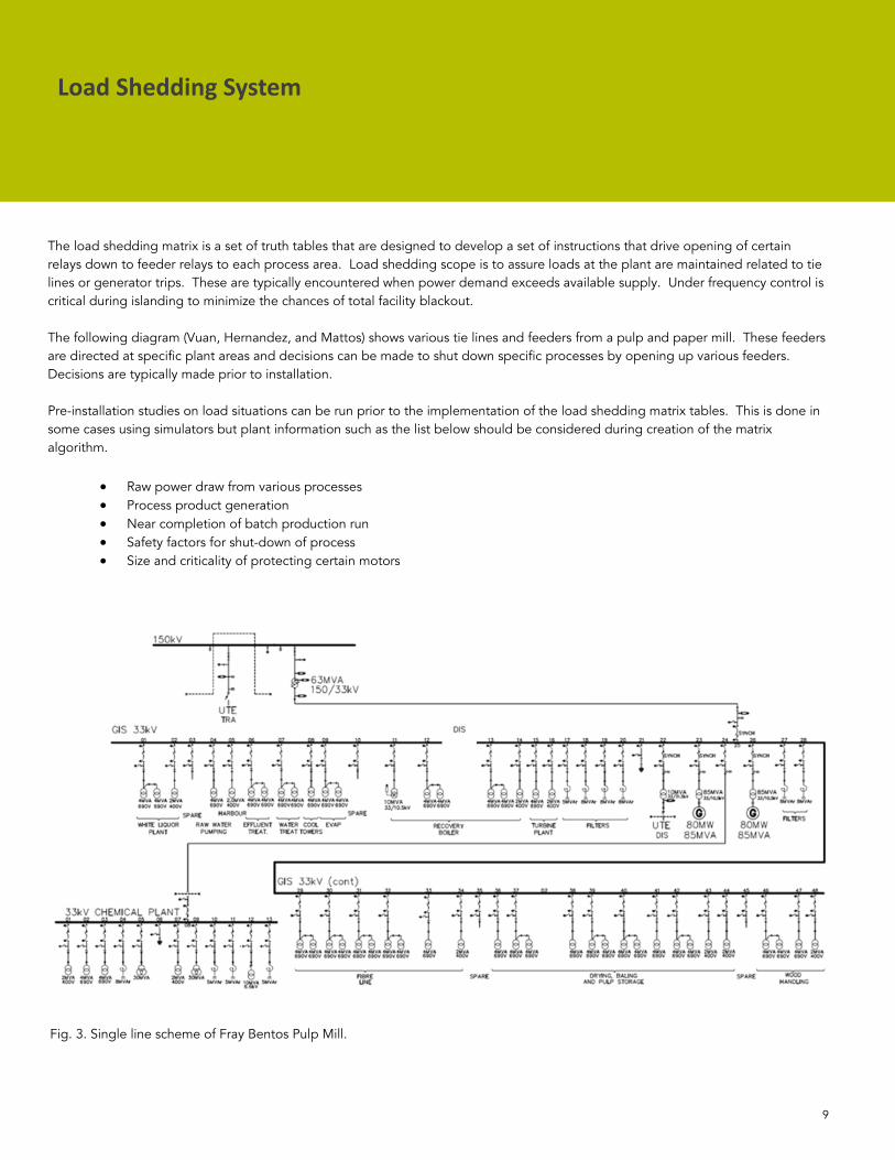
The load shedding matrix is a set of truth tables that are designed to develop a set of instructions that drive opening of certain relays down to feeder relays to each process area. Load shedding scope is to assure loads at the plant are maintained related to tie lines or generator trips. These are typically encountered when power demand exceeds available supply. Under frequency control is critical during islanding to minimize the chances of total facility blackout. The following diagram (Vuan, Hernandez, and Mattos) shows various tie lines and feeders from a pulp and paper mill. These feeders are directed at specific plant areas and decisions can be made to shut down specific processes by opening up various feeders. Decisions are typically made prior to installation. Pre-installation studies on load situations can be run prior to the implementation of the load shedding matrix tables. This is done in some cases using simulators but plant information such as the list below should be considered during creation of the matrix algorithm.

Raw power draw from various processes Process product generation Near completion of batch production run Safety factors for shut-down of process Size and criticality of protecting certain motors

Fig. 3. Single line scheme of Fray Bentos Pulp Mill.


9

Elecsolve Power Modeling

1.9 Intelligent Load Shedding Intelligent Load Shedding (Shokooh, Khandelwal, Shokooh, Tastet, Dai, 2005, p. 1) compared basic and intelligent load shedding where ‘automated solutions lack system operating knowledge and are still best-guess methods which typically result in excessive or insufficient load shedding. An intelligent load shedding system can provide faster and optimal load relief by utilizing actual operating conditions and knowledge of past system disturbances’. ILS is the use of numerous variables to effectively shed load where it needs to be shed. Simulation systems can be employed which use knowledge about the process and the system to shed load across various sections of the plant. Intelligent load shedding combines a number of variables to effectively shed load including, real-time date from IEDs, equipment ratings, existing control system logic, and knowledge derived from simulation studies In basic load shedding ‘load priority tables are executed sequentially to curtail blocks of load regardless of the dynamic changes in loading, generation, or operating configuration. The system-wide operating conditions are often missing from the PLC’s decision-making process, resulting in insufficient or excessive load’ Shokooh et al. 2008, p.5). One symptom of the simplified load shedding scheme is that the overall shedding sequence does not take into consideration the entire scope of the power management system. The load shedding is based only on the part of the process that is tied to control system.

2. Elecsolve Power Modeling 2.1 Overview Intelligent load shedding defines smart decision-making regarding loads and the priority of shedding. In order to maximize efficiencies and process continuation, models of various conditions can be simulated to examine the power flow to the process areas. 2.2 Introduction During the engineering stage, power generation and plant system simulators are utilized to test the control system capability and effectiveness, as the actual field devices are not available in the engineering staging facilities and actual system response is thus unknown. An example for electrical system simulator can be used to simulate a system disturbance (such as loss of a generator), the following system condition will occur.

Local controller of on line generators (Generator controller) act to increase the generator output to meet power demand, due to frequency or voltage drop in the system.

Load Management System Load Shedding Control acts to shed non-critical load to ensure sufficient power supply for Train operation.

Based on the transient of the system, Load Management Shedding Power Generation Control acts on generator and OLTC to ensure desired load sharing among all power sources, and to maintain system frequency and bus voltage (when islanded) or to maintain grid import power (when connected to grid).

The system eventually stabilized at its new set points. 2.3 Electrical System Simulator for Testing To prove the control system performs according to designs, a plant power system model is built (using Invensys SimSci Simulation package). The simulator simulates a control processor with field devices, and behaves exactly, in operation, algorithms and configuration setup, as the actual hardware. The control functions are tested on the simulation system during Factory Acceptance Test (FAT). Later during Site Acceptance Test (SAT), it is shown that the system behaves very close to the test condition and commissioning has been smooth without imposing any difficulties to the actual equipment and system. The simulator can remain available on site for Operator Training and familiarization, and for ongoing fine tuning of applications by Electrical Engineers.

10

2.4 Electrical Operator Training Simulator The operator training is critical for operational safety and profitable plant operation – to do the right thing at the right time. Uncontrolled upsets can cause start-up delays, production outages, severe equipment damage, even catastrophic failures. The functionality of the simulator used during testing and commissioning can be extended to become a fully fledged Operator Training Simulator (OTS). In addition to the full feature of classroom training system, the emphasis is to have the simulation system behave exactly the same as actual hardware and software. The operator will be able to practice the routine operation procedure, such as opening and closing of a circuit breaker, as well as advanced operation, such as power generation control, load shedding control and synchronization operation.

2.5 Elecsolve ElecSolve software adds a DYNSIM library for modeling three phase electrical networks. The solver algorithms make the following important assumptions:

Phases are balanced. Electromagnetic transients happen much faster than solver time steps.

These assumptions provide the ability to solve networks while neglecting electromagnetic transients and out of balance currents. The solver works out a steady state electrical solution at every time step given boundary conditions form the generators and loads.

The electromechanical dynamics are represented in first principles. The complex impedance of each component and transmission line is taken into account.

The library has two co-operating solvers: The Power Flow solver – calculates a consistent set of voltages for the network that satisfies the voltage and load

boundaries. The Machine Dynamics solver - integrates synchronous machine and voltage controller states to solve machine speeds

and AVR dynamics.

At each DYNSIM calculation step the power flow solver is executed before the machine dynamics solver. At the end of the step we arrive at a consistent set of bus voltages, power flow and machine speeds.

3.0 Event Disturbance Record System An Event Disturbance Record System consists of the following two components:

Disturbance Data Collection and Storage Automatic Disturbance event Report generating

3.1 Disturbance Data Collection and Storage The Event Disturbance Record (EDR) System is designed to record and acknowledge alarms and trips, transient voltage and frequency excursions, status changes of breakers and trip units, and to record data before, during, and after these events. The events should be monitored continuously and monitor all protective relays and other devices. A very critical element of the Event Disturbance Record system is time synchronization. Time synchronization can be done directly at

Event Disturbance Record System

11


Local RTU. This significantly minimizes costs from GPS clocks and wiring. Since the local RTU holds the time synchronized data it is also available at the Master SCADA Station. It is typically recommended that the time synchronized data be made available manually or on detection of an event. The Event Disturbance Record System utilizes the DNP3 event system to collect information from various Intelligent Electrical Devices (IED) into the SCD5200 RTU Station Control Devices. As events occur, these are collected and then transferred to the master station, where the events are recorded in the standard Historian and Alarm Database. Each Local RTU records the events independently in the SCD5200 and sends the data to the centralized Historian for permanent storage. The data points and event definition are configured in SCD5200 as well as in the Integrated Development Environment (IDE) and Historian. The Historian collects data associated with events. In many cases the Historian is not on the same computer as the post event package although all the points associated with a particular event have to be in the same historian server.

3.2 Event Disturbance Reporting The Event disturbance reporting function is provided by the InFusion Post Event Report package.

3.2.1 Overview The Post Event Report package is a decision support tool which aids in the analysis of system operations before and after an event. An event can be defined as any data point monitored by the system, either internal in the control system, or in the process, production, or SCADA system. Examples of the types of data which are monitored include equipment going offline or a unit trip or a breaker trip. A Post Event Report package will generate a report based on the historical data related to the event from the historian database. For example, after a boiler goes off line, the user will be able to inquire about the history of its temperature, pressure, electricity usage, and other variables for the moment immediately before it went down. The report generation is executed automatically by an ArchestrA object. The reports are saved in pre-defined location for any users to access. The configuration attributes of the Post Event Report object are described in detail in Table 1. An ArchestrA object tool is an ideal way to manage a package of information. The ArchestrA object is designed to include all the User Defined Attributes associated with the Post Event Report package. The object is assigned to each device and should the report need to be changed, the change can be made in the object template and deployed to any combination of the devices. This provides a huge advantage to the user in terms of (a) lowering the risk or errors in matching of tags to reports and historian event database; (b) lowering the cost to make the engineering changes; and (c) creating consistent reports from engineer to engineer by virtue of an approved template that is accessed by in a template toolbox. 3.2.2 Event Trigger The trigger for an event is monitored by the Historian event tag defined in the report. The Post Event Report program periodically checks the event history in Historian database and once a new event is detected, the program shall wait until the Historian collects enough data for the post event information. The Post Event Report object also provides an attribute for the time interval for both before and after the event which can be configured for each report.

12

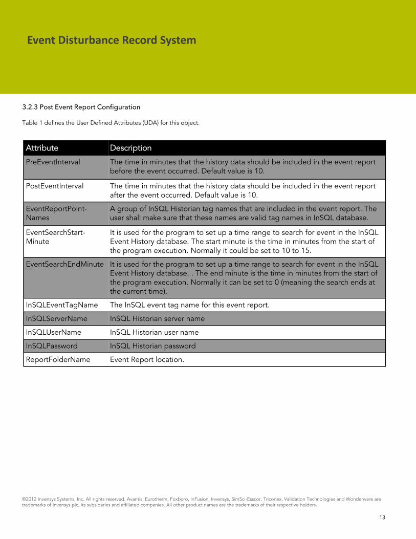
3.2.3 Post Event Report Configuration Table 1 defines the User Defined Attributes (UDA) for this object.

Attribute Description

PreEventInterval The time in minutes that the history data should be included in the event report before the event occurred. Default value is 10.

PostEventInterval The time in minutes that the history data should be included in the event report after the event occurred. Default value is 10.

EventReportPoint-Names

A group of InSQL Historian tag names that are included in the event report. The user shall make sure that these names are valid tag names in InSQL database.

EventSearchStart-Minute

It is used for the program to set up a time range to search for event in the InSQL Event History database. The start minute is the time in minutes from the start of the program execution. Normally it could be set to 10 to 15.

EventSearchEndMinute It is used for the program to set up a time range to search for event in the InSQL Event History database. . The end minute is the time in minutes from the start of the program execution. Normally it can be set to 0 (meaning the search ends at the current time).

InSQLEventTagName The InSQL event tag name for this event report.

InSQLServerName InSQL Historian server name

InSQLUserName InSQL Historian user name

InSQLPassword InSQL Historian password

ReportFolderName Event Report location.


13

©2012 Invensys Systems, Inc. All rights reserved. Avantis, Eurotherm, Foxboro, InFusion, Invensys, SimSci-Esscor, Triconex, Validation Technologies and Wonderware are trademarks of Invensys plc, its subsidaries and affiliated companies. All other product names are the trademarks of their respective holders.

what’s inside - invensysiom.invensys.com/en/pdflibrary/whitepaper_loadsheddingand... · load...

Documents