wenting zhou, weichen wu, nathan palmer, emily mower, noah daniels, lenore cowen, anselm blumer...
TRANSCRIPT
Wenting Zhou, Weichen Wu, Nathan Palmer, Emily Mower, Noah
Daniels, Lenore Cowen, Anselm Blumer
Tufts Universityhttp://camda.cs.tufts.edu
Microarray Data Analysis of Adenocarcinoma Patients’ Survival Using ADC and K-Medians Clustering

Overview Goals Introduction Explanation of ADC and NSM Explanation of MVR, K-Medians,
and Hierarchical Clustering Results Conclusions
Goals
Start with a classification of patients into high-risk and low-risk clusters
Obtain a small subset of genes that still leads to good clusters
These genes may be biologically significant One can use statistical or machine learning
techniques on the reduced set that would have led to overfitting on the original set
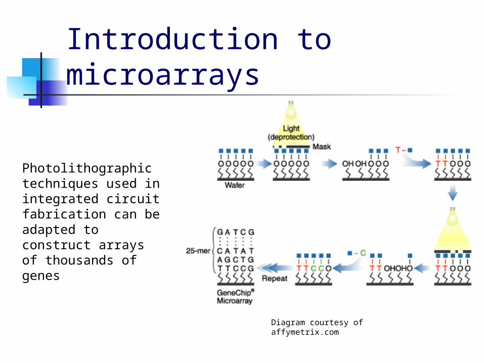
Introduction to microarrays
Photolithographic techniques used in integrated circuit fabrication can be adapted to construct arrays of thousands of genes
Diagram courtesy of affymetrix.com
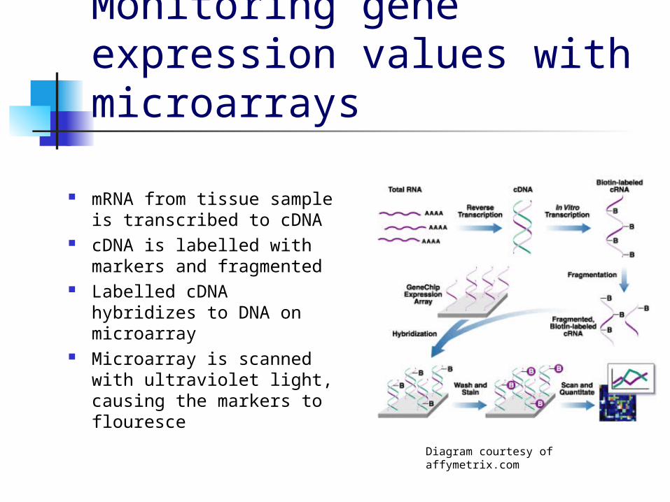
Monitoring gene expression values with microarrays
mRNA from tissue sample is transcribed to cDNA
cDNA is labelled with markers and fragmented
Labelled cDNA hybridizes to DNA on microarray
Microarray is scanned with ultraviolet light, causing the markers to flouresce
Diagram courtesy of affymetrix.com
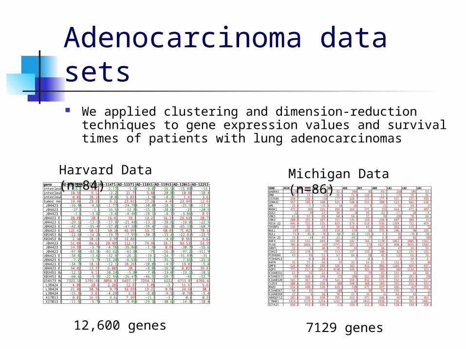
Adenocarcinoma data sets We applied clustering and dimension-reduction
techniques to gene expression values and survival times of patients with lung adenocarcinomas
GENE AD10 AD2 AD3 AD5 AD6 AD7 AD8 L01 L02 L04GABRA3 170 59.7 80 92.4 104 88 69.7 230 105 53.7OMD 69.4 18.1 26 96.9 72.8 138.6 11.1 176 78.1 36.7GS3686 250.7 146.8 150 177.8 228.7 115.5 177.8 511.3 233.9 393.6SEMA3C 957.1 186.8 340.2 515.8 540.8 616.6 380.5 523.9 602.7 160.5GML 25.4 -7.7 -16.3 18 26 9 21 32 24.3 27MKNK1 471.2 309 225.7 296.6 264.1 371.9 291 664.2 471.6 407.3OGG1 -52 -99 23.5 48.5 -10 49.2 -62.5 -17.1 20 -4.4VRK1 42.8 57.9 69.4 60.4 56.4 37.2 99 295 78.1 94.2VRK2 200.9 151.5 207.6 151.5 145.9 149.2 238.8 607.2 300.7 411RES4-22 846.4 722.8 515.1 819.1 674.4 618.9 936.2 1388.1 732.1 959.1SH3BP2 134.7 55.3 63.7 56.3 122.6 49.2 139.3 362.5 115.5 52NULL 147 131.2 107 118.9 174 92 175.9 396.9 90 185.3NULL -71.4 -85.4 -78.3 -80.7 -85.2 -135.3 4.1 46 -76.4 -50.2RES4-25 19.6 -44 49.2 22.2 -69.2 17 6.8 60 81 105RNF4 953.2 552.1 609.4 708.2 582.7 768.1 1130.1 1062.6 1005.8 1561.9PLAB 703.6 2068.7 447 2771.2 327.1 179 1427.8 460.4 3691.9 1583.4ARNTL 22.2 -22 30.8 75.5 32 57 28.2 47 34.8 34.3CDH23 222.2 178.3 99 111.6 157.1 133.2 340.2 325 131.9 181.5PCDHGB4 43.5 69 53.4 67.6 66.8 60 45.8 125 66.8 76.4PCDHGA12 -7 -0.8 28.4 4.2 3 -0.6 6.8 1 10.4 2.3H4FM 95.5 75.1 68.5 57 35.5 54.5 55.1 152.6 71.1 88GMFB 526.9 391.8 288.9 326.1 383.1 416.4 806.9 1286.3 669.6 437.3AQP3 777.5 517.9 1053.2 4190.3 449.5 421.9 709.9 687 1194.1 413.8KIAA0316 62.3 52 24.8 43.8 31 39 45.8 162.6 44 48.5KIAA0317 149 328.6 199.4 172 288 321.4 238.8 314.7 201.8 298KIAA0320 565.7 467.2 378 522.1 558.9 432.1 571.7 592.4 493.8 517.2CLOCK 400.6 259.7 238.5 400 340.5 360.3 189.1 365.3 252.6 433.8MADD 554.6 480.9 528.7 618.6 530 471.1 597.3 486.3 427 393.6KIAA0367 68.5 65 16 108 32 98 95.8 195.1 52.8 15KIAA0368 22.2 4 10.8 70.2 23.5 35.5 41 84.6 43 31ARHGEF12 281.6 355.7 650.7 795.5 412.5 371.9 246.8 437 375.8 454.9CTNND1 1018.2 1579.4 1254.4 1293.3 1220 1053.2 1098.5 738.6 703.6 3401.2SCYA21 658.2 419.8 319.3 172 358.5 315.2 426.1 510.5 190.8 350.6
gene AD-043T2-A7-1AD-111T2-A8-1AD-114T1-A9-1 *AD-115T1-A12-1 *AD-118t1-A13-1AD-119t3-A195-8AD-120t1-A226-8 *AD-122t3-A197-8interleukin 2 -18.6 9.12 -2.175 -1.54 -9.07 -16.58 -15.895 -14.5interleukin 10 10.54 9.12 -2.21 21.75 3.08 -20.09 10.88 -10.48interleukin 4 0.01 10.18 -0.06 5.835 -1.98 -8.39 1.61 3.61tumor necrosis factor receptor superfamily, member 619.44 29.29 6.32 23.815 17.26 4.49 23.845 12.67 J04423 E coli bioB gene biotin synthetase (-5, -M, -3 represent transcript regions 5 prime, Middle, and 3 prime respectively) -16.98 -4.68 -1.775 -24.785 -10.09 -18.92 -21.98 -17.52 J04423 E coli bioB gene biotin synthetase (-5, -M, -3 represent transcript regions 5 prime, Middle, and 3 prime respectively) -27.5 -1.5 -16.53 -12.89 -15.15 -20.09 -29 -20.54 J04423 E coli bioB gene biotin synthetase (-5, -M, -3 represent transcript regions 5 prime, Middle, and 3 prime respectively) -1.6 -3.62 -3.61 -4.485 -18.19 -8.39 -3.865 0.59J04423 E coli bioC protein (-5 and -3 represent transcript regions 5 prime and 3 prime respectively)38.88 20.8 16.41 19.5 13.21 16.19 23.635 28.78J04423 E coli bioC protein (-5 and -3 represent transcript regions 5 prime and 3 prime respectively)-29.12 -13.18 -17.97 -21.445 -13.13 -38.82 -19.01 -22.55J04423 E coli bioD gene dethiobiotin synthetase (-5 and -3 represent transcript regions 5 prime and 3 prime respectively)-42.87 -35.47 -57.02 -47.205 -39.47 -56.38 -65.195 -68.78J04423 E coli bioD gene dethiobiotin synthetase (-5 and -3 represent transcript regions 5 prime and 3 prime respectively)121.62 50.53 59.36 46.995 53.71 68.85 71.025 78.18X03453 Bacteriophage P1 cre recombinase protein (-5 and -3 represent transcript regions 5 prime and 3 prime respectively)-22.64 -14.24 -19.73 -7.555 -30.35 -15.41 -22.815 -22.55X03453 Bacteriophage P1 cre recombinase protein (-5 and -3 represent transcript regions 5 prime and 3 prime respectively)2.44 10.18 2.99 12.885 -3 -4.87 0.965 4.62 J04423 E coli bioB gene biotin synthetase (-5, -M, -3 represent transcript regions 5 prime, Middle, and 3 prime respectively) 51.04 86.63 29.485 112.72 74.96 19.71 93.535 54.99 J04423 E coli bioB gene biotin synthetase (-5, -M, -3 represent transcript regions 5 prime, Middle, and 3 prime respectively) 14.59 -5.74 -4.765 -35.865 -1.98 0.98 -30.79 -35.62 J04423 E coli bioB gene biotin synthetase (-5, -M, -3 represent transcript regions 5 prime, Middle, and 3 prime respectively) -97.84 -43.96 -65.625 -61.04 -79 -56.38 -97.25 -111.96J04423 E coli bioC protein (-5 and -3 represent transcript regions 5 prime and 3 prime respectively)-38.82 -3.62 -32.87 -26.21 -19.2 -24.77 -31.695 -31.6J04423 E coli bioC protein (-5 and -3 represent transcript regions 5 prime and 3 prime respectively)-7.27 -5.74 -11.285 -6.535 -11.1 -35.31 -7.655 -25.56J04423 E coli bioD gene dethiobiotin synthetase (-5 and -3 represent transcript regions 5 prime and 3 prime respectively)-34.78 10.18 -12.12 18.265 -10.09 -4.87 19.03 -5.45J04423 E coli bioD gene dethiobiotin synthetase (-5 and -3 represent transcript regions 5 prime and 3 prime respectively)34.02 13.37 6.805 20.2 -8.06 -16.58 8.025 39.87X03453 Bacteriophage P1 cre recombinase protein (-5 and -3 represent transcript regions 5 prime and 3 prime respectively)-12.13 9.12 -10.245 -5.04 -7.05 -13.07 -13.15 -18.52X03453 Bacteriophage P1 cre recombinase protein (-5 and -3 represent transcript regions 5 prime and 3 prime respectively)-60.66 -9.99 -22.565 -26.475 -46.57 -58.73 -46 -52.71U14573 Human Alu-Sq subfamily consensus sequence.7322.58 5795.86 8056.02 6437.37 7254.32 6222 6715.07 6766.43 L38424 B subtilis dapB, jojF, jojG genes corresponding to nucleotides 1358-3197 of L38424 (-5, -M, -3 represent transcript regions 5 prime, Middle, and 3 prime respectively) 4.06 20.8 2.285 12.87 1.06 -3.7 11.67 5.63 L38424 B subtilis dapB, jojF, jojG genes corresponding to nucleotides 1358-3197 of L38424 (-5, -M, -3 represent transcript regions 5 prime, Middle, and 3 prime respectively) 21.06 30.36 9.79 32.835 13.21 0.98 24.68 30.8 L38424 B subtilis dapB, jojF, jojG genes corresponding to nucleotides 1358-3197 of L38424 (-5, -M, -3 represent transcript regions 5 prime, Middle, and 3 prime respectively) -15.36 3.81 -4.295 3.38 -6.03 -9.56 -0.745 -5.45 X17013 B subtilis lys gene for diaminopimelate decarboxylase corresponding to nucleotides 350-1345 of X17013 (-5, -M, -3 represent transcript regions 5 prime, Middle, and 3 prime respectively) 0.01 16.55 4.62 7.395 -11.1 -3.7 0.6 0.59 X17013 B subtilis lys gene for diaminopimelate decarboxylase corresponding to nucleotides 350-1345 of X17013 (-5, -M, -3 represent transcript regions 5 prime, Middle, and 3 prime respectively) -11.32 -5.74 -11.15 -9.455 -23.26 -30.63 -14.36 -10.48
Harvard Data (n=84)
Michigan Data (n=86)
12,600 genes 7129 genes
Overview Goals Introduction Explanation of ADC and NSM Explanation of MVR, K-Medians,
and Hierarchical Clustering Results Conclusions
ADC and NSM Overview We use Approximate Distance
Clustering maps (Cowen, 1997) to project the data into one or two dimensions so we can use very simple clustering techniques.
Then we use Nearest Shrunken Mean (Tibshirani, 1999) to reduce the number of genes used to predict the clusters.
We evaluate using leave-one-out crossvalidation and log-rank tests
Approximate Distance Clustering (ADC, Cowen 1997) Approximate Distance Clustering is a
method that reduces the dimensionality of the data.
This is done by calculating the distance from each datapoint to a subset of the data, which is called a witness set.
A different witness set is used for each desired dimension
A simple clustering technique is used on the projected data
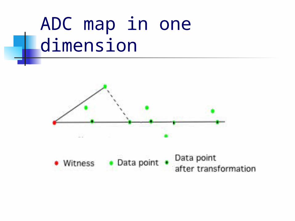
ADC map in one dimension
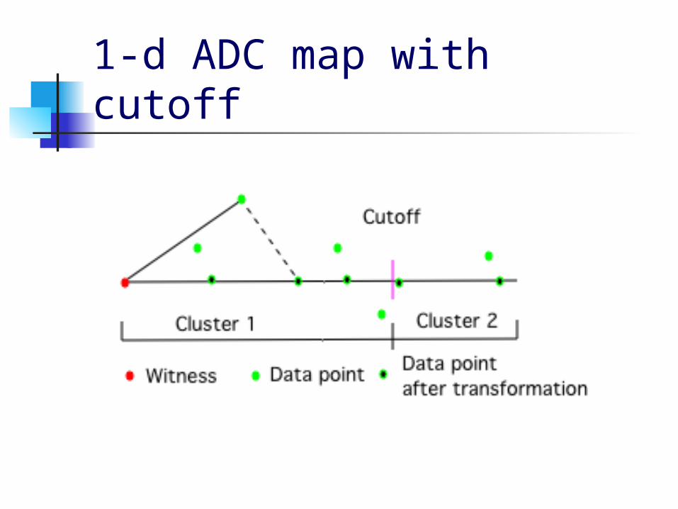
1-d ADC map with cutoff
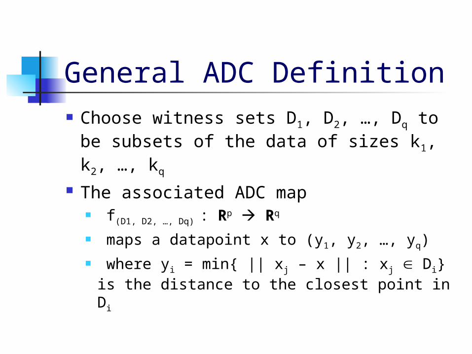
General ADC Definition Choose witness sets D1, D2, …, Dq to
be subsets of the data of sizes k1, k2, …, kq
The associated ADC map f(D1, D2, …, Dq) : Rp Rq maps a datapoint x to (y1, y2, …, yq) where yi = min{ || xj – x || : xj Di} is
the distance to the closest point in Di
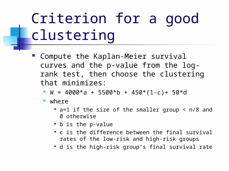
Criterion for a good clustering Compute the Kaplan-Meier survival curves
and the p-value from the log-rank test, then choose the clustering that minimizes:
W = 4000*a + 5500*b + 450*(1-c)+ 50*d where
a=1 if the size of the smaller group < n/8 and 0 otherwise
b is the p-value c is the difference between the final survival rates of
the low-risk and high-risk groups d is the high-risk group’s final survival rate
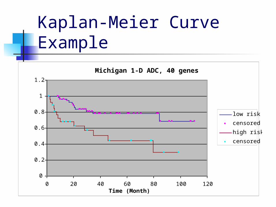
Kaplan-Meier Curve Example
Michigan 1-D ADC, 40 genes
0
0.2
0.4
0.6
0.8
1
1.2
0 20 40 60 80 100 120Time (Month)
Survival Rate
low risk
censored
high risk
censored
Nearest Shrunken Mean (NSM) Gene Reduction (Tibshirani,1999)
NSM eliminates genes with cluster means close to the overall mean.
NSM shrinks the cluster means toward the overall mean by an amount proportional to the within-class standard deviations for each gene.
If the cluster means all reach the overall mean, that gene can be eliminated.
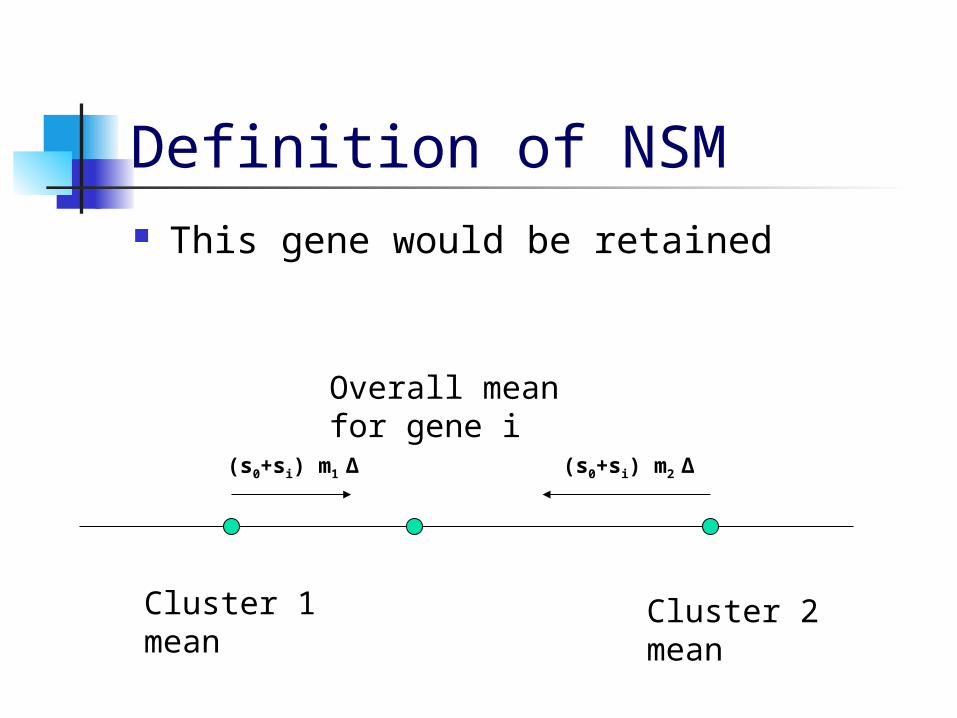
Definition of NSM This gene would be retained
Overall meanfor gene i
Cluster 1mean
Cluster 2mean
(s0+si) m1 ∆ (s0+si) m2 ∆
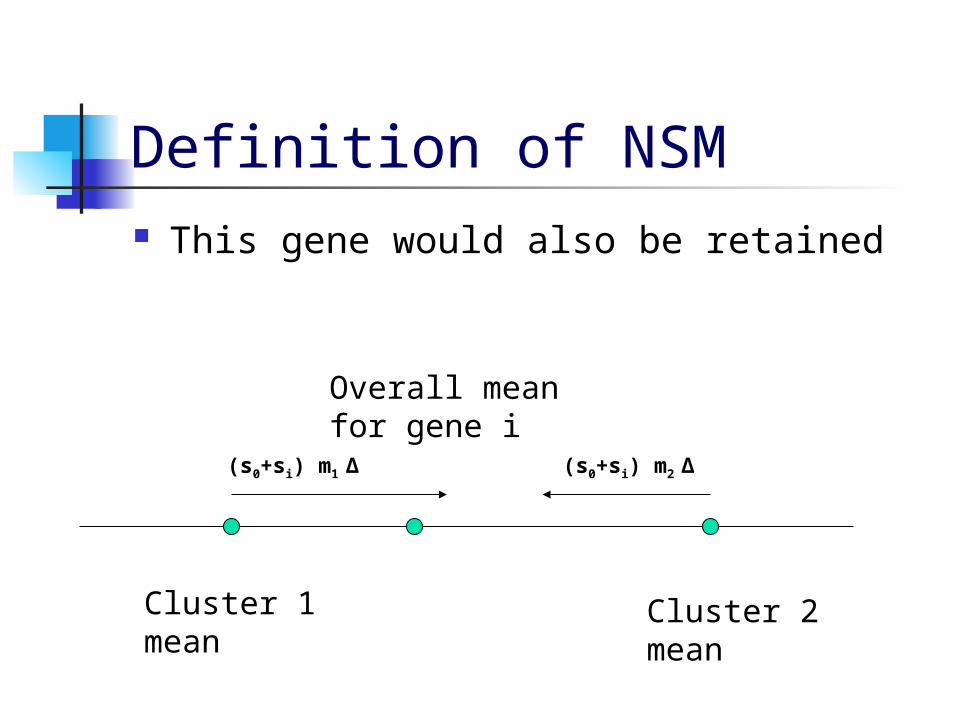
Definition of NSM This gene would also be retained
Overall meanfor gene i
Cluster 1mean
Cluster 2mean
(s0+si) m1 ∆ (s0+si) m2 ∆
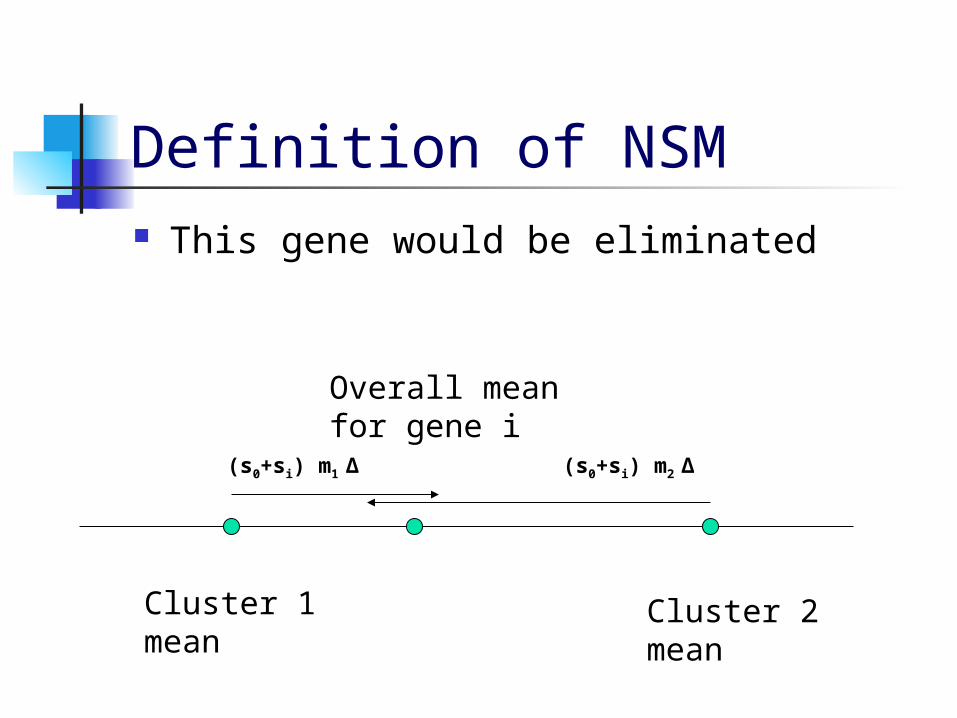
Definition of NSM This gene would be eliminated
Overall meanfor gene i
Cluster 1mean
Cluster 2mean
(s0+si) m1 ∆ (s0+si) m2 ∆
Overview Goals Introduction Explanation of ADC and NSM Explanation of MVR, K-Medians,
and Hierarchical Clustering Results Conclusions
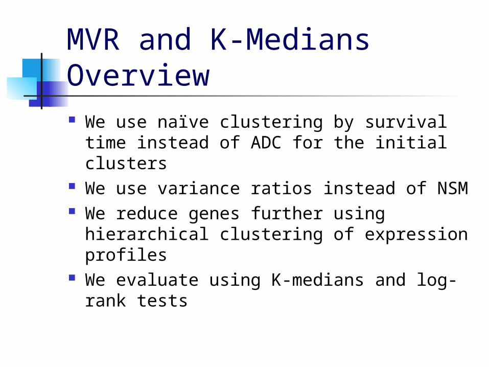
MVR and K-Medians Overview We use naïve clustering by survival time
instead of ADC for the initial clusters We use variance ratios instead of NSM We reduce genes further using
hierarchical clustering of expression profiles
We evaluate using K-medians and log-rank tests
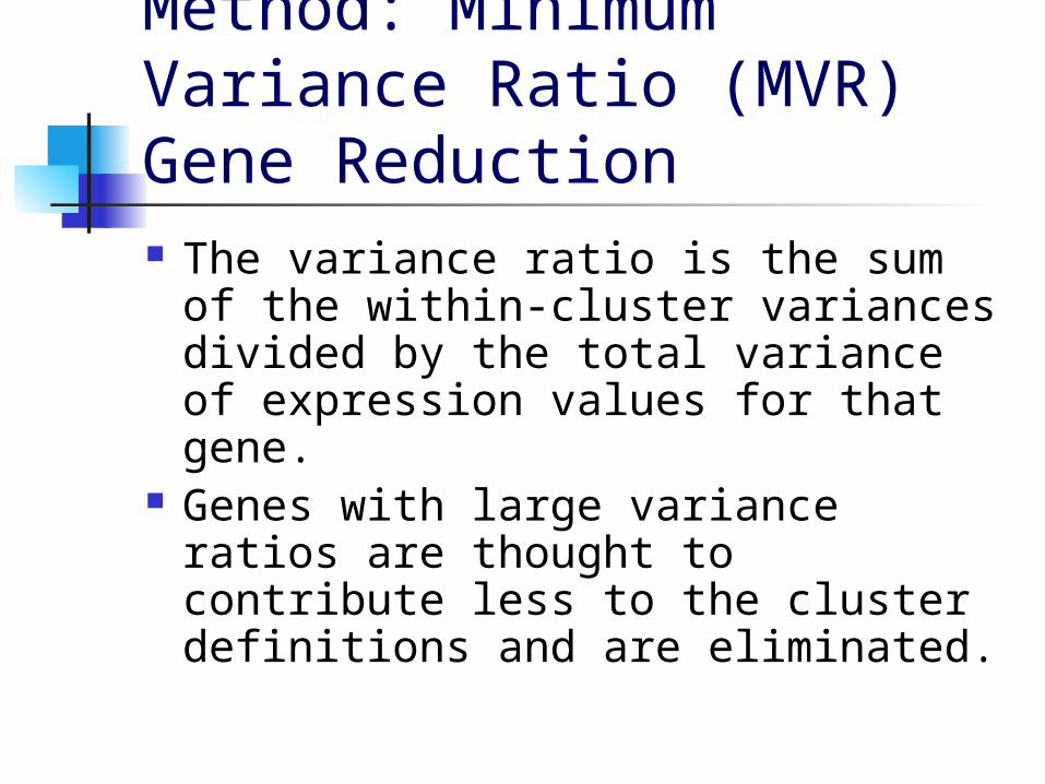
Method: Minimum Variance Ratio (MVR) Gene Reduction The variance ratio is the sum of
the within-cluster variances divided by the total variance of expression values for that gene.
Genes with large variance ratios are thought to contribute less to the cluster definitions and are eliminated.
Hierarchical Clustering of Genes Different genes may have similar
expression profiles Eliminating similar genes may lead to a
smaller set of genes that still leads to a good separation into high-risk and low-risk clusters
Hierarchically cluster the genes until the desired number of clusters is obtained, then select one gene from each cluster
K-Medians Clustering This unsupervised clustering method
finds the K datapoints that are the best cluster centers
In this paper we use K=2 so it is possible to find the optimal clustering by trying all possible pairs of points as cluster centers.
The quality of the clustering is calculated as the total distance of data points to their cluster centers
Overview Goals Introduction Explanation of ADC and NSM Explanation of MVR, K-Medians,
and Hierarchical Clustering Results Conclusions
Experimental Results The following tables give the results obtained
when using the W criterion to select the best ADC witnesses and cutoffs, then reducing the set of probesets with NSM.
The p-values were obtained from leave-one-out crossvalidation on the reduced set of probesets.
The values for STCC were obtained by following the same procedure but substituting clusters formed from the 50% or 60% highest risk patients for the ADC clusters.
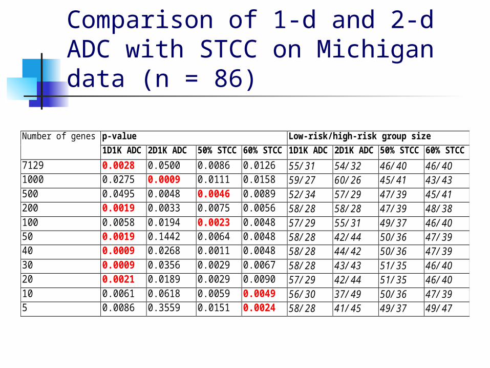
Comparison of 1-d and 2-d ADC with STCC on Michigan data (n = 86)
p-value Low-risk/high-risk group sizeNumber of genes
1D1K ADC 2D1K ADC 50% STCC 60% STCC 1D1K ADC 2D1K ADC 50% STCC 60% STCC
7129 0.0028 0.0500 0.0086 0.0126 55/31 54/32 46/40 46/401000 0.0275 0.0009 0.0111 0.0158 59/27 60/26 45/41 43/43500 0.0495 0.0048 0.0046 0.0089 52/34 57/29 47/39 45/41200 0.0019 0.0033 0.0075 0.0056 58/28 58/28 47/39 48/38100 0.0058 0.0194 0.0023 0.0048 57/29 55/31 49/37 46/4050 0.0019 0.1442 0.0064 0.0048 58/28 42/44 50/36 47/3940 0.0009 0.0268 0.0011 0.0048 58/28 44/42 50/36 47/3930 0.0009 0.0356 0.0029 0.0067 58/28 43/43 51/35 46/4020 0.0021 0.0189 0.0029 0.0090 57/29 42/44 51/35 46/4010 0.0061 0.0618 0.0059 0.0049 56/30 37/49 50/36 47/395 0.0086 0.3559 0.0151 0.0024 58/28 41/45 49/37 49/47
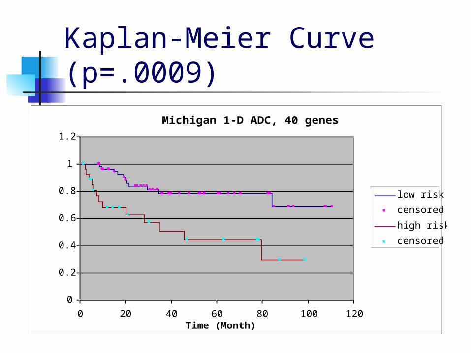
Kaplan-Meier Curve (p=.0009)
Michigan 1-D ADC, 40 genes
0
0.2
0.4
0.6
0.8
1
1.2
0 20 40 60 80 100 120Time (Month)
Survival Rate
low risk
censored
high risk
censored
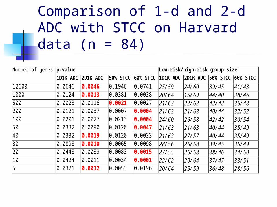
Comparison of 1-d and 2-d ADC with STCC on Harvard data (n = 84)
p-value Low-risk/high-risk group sizeNumber of genes
1D1K ADC 2D1K ADC 50% STCC 60% STCC 1D1K ADC 2D1K ADC 50% STCC 60% STCC
12600 0.0646 0.0046 0.1946 0.0741 25/59 24/60 39/45 41/431000 0.0124 0.0013 0.0381 0.0038 20/64 15/69 44/40 38/46500 0.0023 0.0116 0.0021 0.0027 21/63 22/62 42/42 36/48200 0.0121 0.0037 0.0007 0.0004 21/63 21/63 40/44 32/52100 0.0201 0.0027 0.0213 0.0004 24/60 26/58 42/42 30/5450 0.0332 0.0090 0.0120 0.0047 21/63 21/63 40/44 35/4940 0.0332 0.0019 0.0120 0.0033 21/63 27/57 40/44 35/4930 0.0898 0.0010 0.0065 0.0098 28/56 26/58 39/45 35/4920 0.0448 0.0039 0.0083 0.0015 27/55 26/58 38/46 34/5010 0.0424 0.0011 0.0034 0.0001 22/62 20/64 37/47 33/515 0.0321 0.0032 0.0053 0.0196 20/64 25/59 36/48 28/56
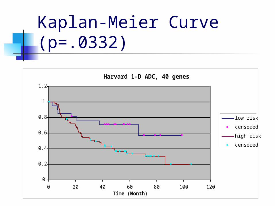
Kaplan-Meier Curve (p=.0332)
Harvard 1-D ADC, 40 genes
0
0.2
0.4
0.6
0.8
1
1.2
0 20 40 60 80 100 120Time (Month)
Survival Rate
low risk
censored
high risk
censored
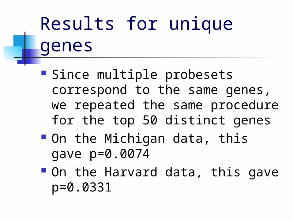
Results for unique genes Since multiple probesets
correspond to the same genes, we repeated the same procedure for the top 50 distinct genes
On the Michigan data, this gave p=0.0074
On the Harvard data, this gave p=0.0331
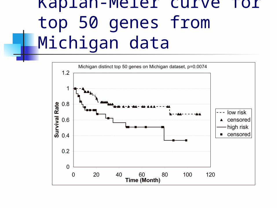
Kaplan-Meier curve for top 50 genes from Michigan data
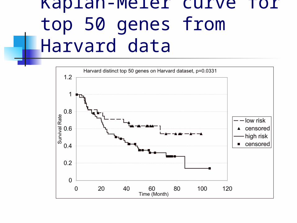
Kaplan-Meier curve for top 50 genes from Harvard data
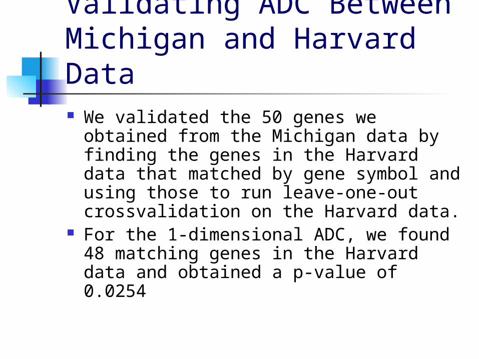
Validating ADC Between Michigan and Harvard Data We validated the 50 genes we obtained
from the Michigan data by finding the genes in the Harvard data that matched by gene symbol and using those to run leave-one-out crossvalidation on the Harvard data.
For the 1-dimensional ADC, we found 48 matching genes in the Harvard data and obtained a p-value of 0.0254
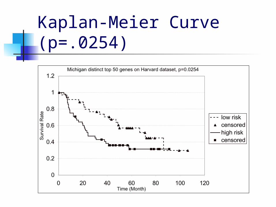
Kaplan-Meier Curve (p=.0254)
Validating ADC Between Validating ADC Between Michigan and Harvard Michigan and Harvard DataData We validated the 50 genes we obtained We validated the 50 genes we obtained
from the Harvard data by finding the from the Harvard data by finding the genes in the Michigan data that genes in the Michigan data that matched by gene symbol and using matched by gene symbol and using those to run leave-one-out those to run leave-one-out crossvalidation on the Michigan data. crossvalidation on the Michigan data.
For the 1-dimensional ADC, we found 42 For the 1-dimensional ADC, we found 42 matching genes in the Michigan data matching genes in the Michigan data and obtained a p-value of 0.0307and obtained a p-value of 0.0307
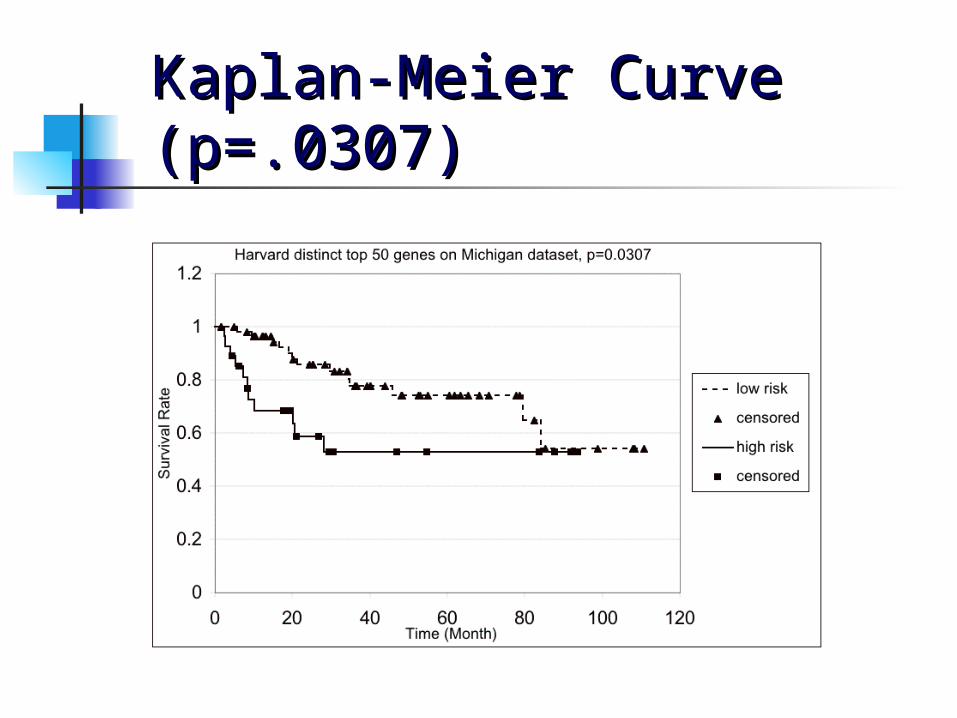
Kaplan-Meier Curve Kaplan-Meier Curve (p=.0307)(p=.0307)
Some cancer-related genes found on our top-50 list, but not found in the Michigan top-50
SPARCL1 (also known as MAST9 or hevin) - down regulation of SPARCL1 also occurs in prostate and colon carcinomas, suggesting that SPARCL1 inactivation is a common event not only in NSCLCs but also in other tumors of epithelial origin.
CD74 - well-known for expression in cancers PRDX1 - linked to tumor prevention PFN2 - seen as increasing in gastric cancer tissues SFTPC - responsible for morphology of the lung; a
mutation causes chronic lung disease HLA-DRA (HLA-A) - lack of expression causes cancers
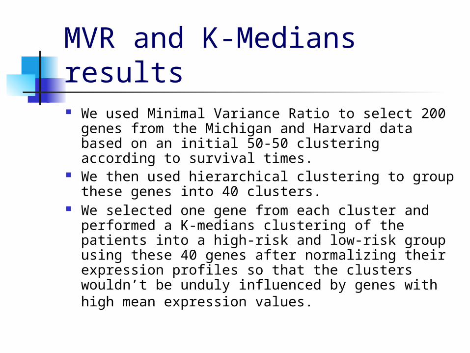
MVR and K-Medians results We used Minimal Variance Ratio to select 200
genes from the Michigan and Harvard data based on an initial 50-50 clustering according to survival times.
We then used hierarchical clustering to group these genes into 40 clusters.
We selected one gene from each cluster and performed a K-medians clustering of the patients into a high-risk and low-risk group using these 40 genes after normalizing their expression profiles so that the clusters wouldn’t be unduly influenced by genes with high mean expression values.
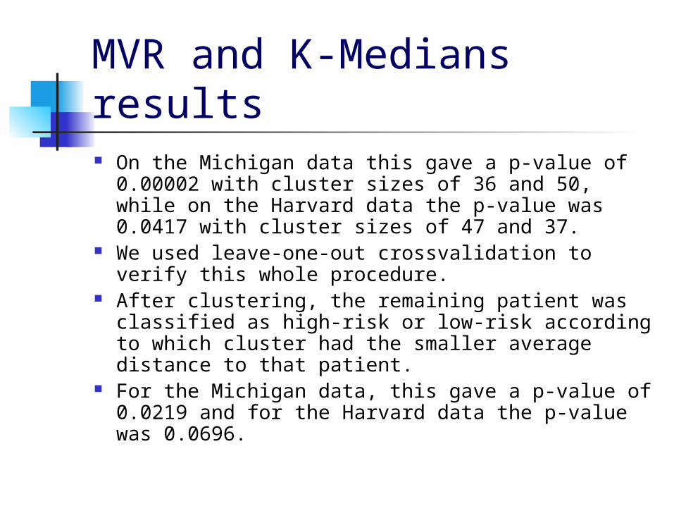
MVR and K-Medians results On the Michigan data this gave a p-value of
0.00002 with cluster sizes of 36 and 50, while on the Harvard data the p-value was 0.0417 with cluster sizes of 47 and 37.
We used leave-one-out crossvalidation to verify this whole procedure.
After clustering, the remaining patient was classified as high-risk or low-risk according to which cluster had the smaller average distance to that patient.
For the Michigan data, this gave a p-value of 0.0219 and for the Harvard data the p-value was 0.0696.
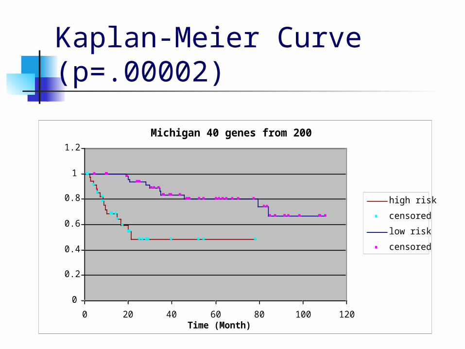
Kaplan-Meier Curve (p=.00002)
Michigan 40 genes from 200
0
0.2
0.4
0.6
0.8
1
1.2
0 20 40 60 80 100 120Time (Month)
Survival Rate
high risk
censored
low risk
censored

Kaplan-Meier Curve (p=.0417)
Harvard 40 genes from 200
0
0.2
0.4
0.6
0.8
1
1.2
0 20 40 60 80 100 120Time (Month)
Survival Rate
low risk
censored
high risk
censored
Conclusion Combinations of simple techniques
yield small sets of genes with high predictive power
Different techniques give different sets of genes
ADC - NSM was often superior to MVR - K-medians - Hierarchical Clustering, but the latter was surprisingly good

Conclusion
The good news:
Much more research remains to be done
Visit http://camda.cs.tufts.edu
Thank you