week 4 ergodic random processes, power spectrum ...users.ece. random processes, power spectrum...

EE4601Communication Systems

Week 4Ergodic Random Processes, Power Spectrum

Linear Systems

0 c2011, Georgia Institute of Technology (lect4 1)

Ergodic Random Processes

An ergodic random process is one where time averages are equal to ensembleaverages. Hence, for all g(X) and X

E[g(X)] =

g(X)pX(t)(x)dx

= limT

1

2T

T

Tg[X(t)]dt

= < g[X(t)] >

For a random process to be ergodic, it must be strictly stationary. However, notall strictly stationary random processes are ergodic.

A random process is ergodic in the mean if

< X(t) >= X

and ergodic in the autocorrelation if

< X(t)X(t+ ) >= XX()

0 c2011, Georgia Institute of Technology (lect4 2)

Example (contd)

Recall the random process

X(t) = A cos(2fct+)

where A and fc are constants, and is a uniformly distributed random phase.

p() =

1/(2) , 0 2

0 , elsewhere

The time average mean of X(t) is

< X(t) >= limT

1

2T

T

TA cos(2fct+ )dt = 0

In this example X(t) =< X(t) >, so the random process X(t) is ergodic in themean.

N.B. Make sure you understand the difference between the time average andensemble average.

0 c2011, Georgia Institute of Technology (lect4 3)

Example (contd)

The time average autocorrelation of X(t) is

< X(t)X(t+ ) > = limT

1

2T

T

TA2 cos(2fct+ 2fc + ) cos(2fct+ )dt

= limT

A2

4T

T

T[cos(2fc) + cos(4fct+ 2fc + 2)] dt

=A2

2cos(2fc)

The random process X(t) is ergodic in the autocorrelation.

It follows that the random process X(t) in this example is ergodic in the meanand autocorrelation.

0 c2011, Georgia Institute of Technology (lect4 4)

Example

Consider the random process shown below.

X (t) = a P = 1/4

P = 1/4

X (t) = 0 P = 1/2

X (t) = -a

1 1

22

3 3

0 c2011, Georgia Institute of Technology (lect4 5)

Example (contd)

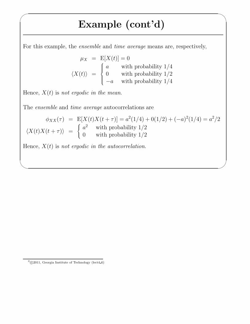
For this example, the ensemble and time average means are, respectively,

X = E[X(t)] = 0

X(t) =

a with probability 1/40 with probability 1/2

a with probability 1/4

Hence, X(t) is not ergodic in the mean.

The ensemble and time average autocorrelations are

XX() = E[X(t)X(t+ )] = a2(1/4) + 0(1/2) + (a)2(1/4) = a2/2

X(t)X(t + ) =

a2 with probability 1/20 with probability 1/2

Hence, X(t) is not ergodic in the autocorrelation.

0 c2011, Georgia Institute of Technology (lect4 6)

Example (contd)

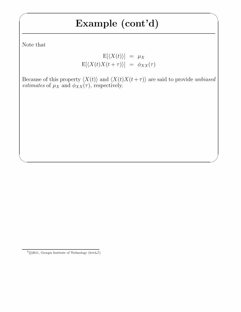
Note that

E[X(t)] = X

E[X(t)X(t+ )] = XX()

Because of this property X(t) and X(t)X(t+ ) are said to provide unbiasedestimates of X and XX(), respectively.

0 c2011, Georgia Institute of Technology (lect4 7)

Power Spectral Density

The power spectral density (psd) of a random process X(t) is the Fourier trans-form of its autocorrelation function, i.e.,

XX(f) = =

XX()e

j2fd

XX() =

XX(f)e

j2fdf .

We have seen that XX() is real and even. Therefore, XX(f) = XX(f)

meaning that XX(f) is also real and even.

The total power (ac + dc), P , in a random process X(t) is

P = E[X2(t)] = XX(0) =

XX(f)df

a famous result known as Parsevals theorem.

0 c2011, Georgia Institute of Technology (lect4 8)

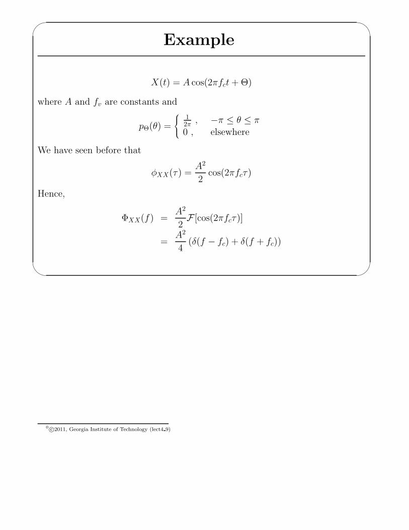
Example

X(t) = A cos(2fct+)

where A and fv are constants and

p() =

12

,

0 , elsewhere

We have seen before that

XX() =A2

2cos(2fc)

Hence,

XX(f) =A2

2F [cos(2fc)]

=A2

4((f fc) + (f + fc))

0 c2011, Georgia Institute of Technology (lect4 9)

Properties of XX(f )

1. XX(0) = XX()d

2. 0+0 XX(f)df = dc power

3. XX(0) =XX(f)df = total power

4. XX(f) 0 for all f . Power is never negative.

5. XX(f) = XX(f) (even function) if X(t) is a real random process.

6. XX(f) is always real.

0 c2011, Georgia Institute of Technology (lect4 10)

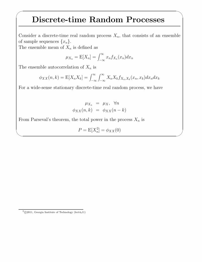
Discrete-time Random Processes

Consider a discrete-time real random process Xn, that consists of an ensembleof sample sequences {xn}.The ensemble mean of Xn is defined as

Xn = E[Xn] =

xnfXn(xn)dxn

The ensemble autocorrelation of Xn is

XX(n, k) = E[XnXk] =

XnXkfXn,Xk(xn, xk)dxndxk

For a wide-sense stationary discrete-time real random process, we have

Xn = X , n

XX(n, k) = XX(n k)

From Parsevals theorem, the total power in the process Xn is

P = E[X2n] = XX(0)

0 c2011, Georgia Institute of Technology (lect4 11)

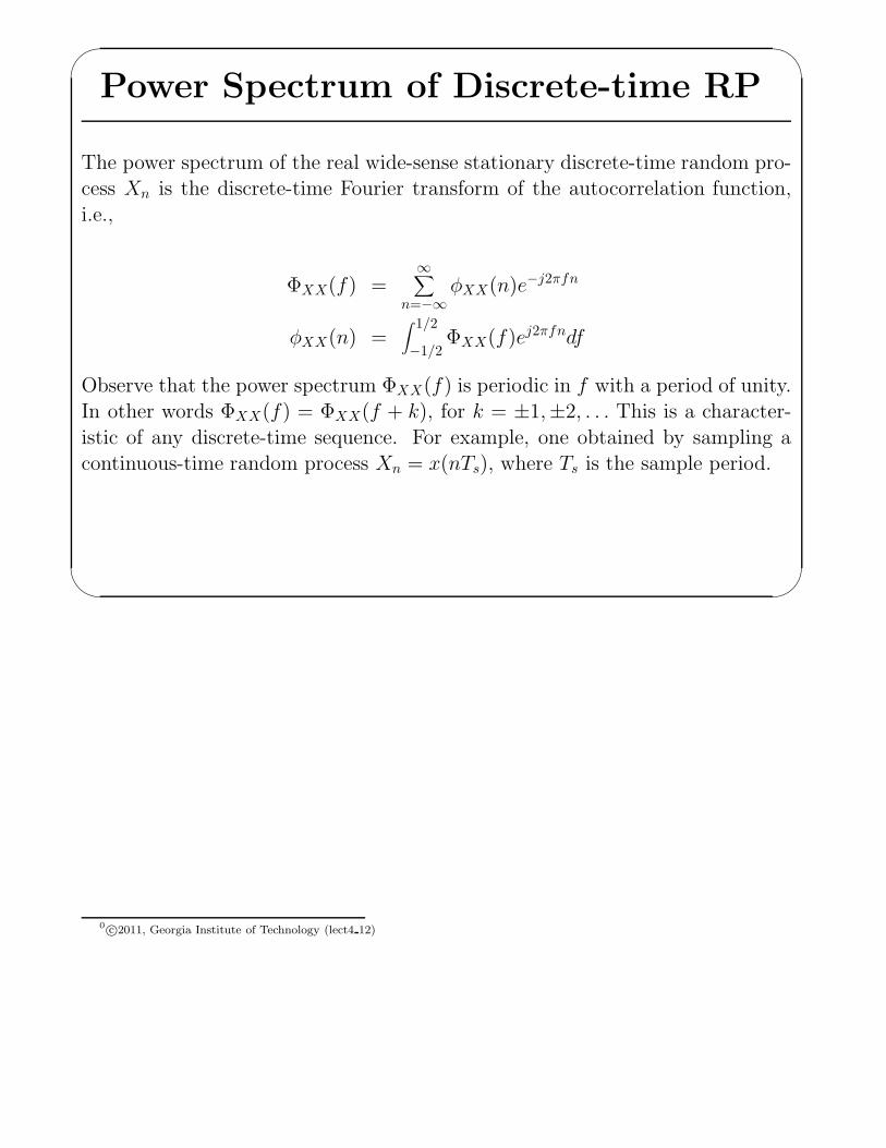
Power Spectrum of Discrete-time RP

The power spectrum of the real wide-sense stationary discrete-time random pro-cess Xn is the discrete-time Fourier transform of the autocorrelation function,

i.e.,

XX(f) =

n=XX(n)e

j2fn

XX(n) = 1/2

1/2XX(f)e

j2fndf

Observe that the power spectrum XX(f) is periodic in f with a period of unity.In other words XX(f) = XX(f + k), for k = 1,2, . . . This is a character-

istic of any discrete-time sequence. For example, one obtained by sampling acontinuous-time random process Xn = x(nTs), where Ts is the sample period.

0 c2011, Georgia Institute of Technology (lect4 12)

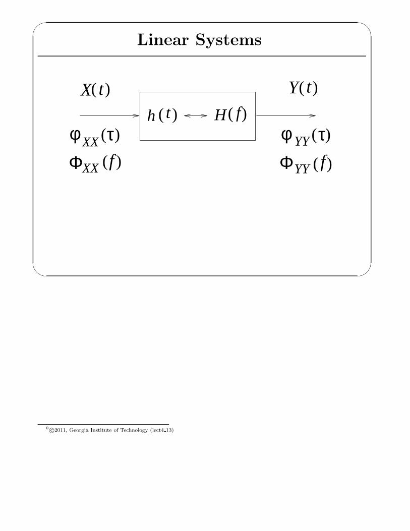
Linear Systems

Yt t

XX

XX

YY

YY

f

t( )h H( )fX( ) ( )

( )

( )

( )f( )

0 c2011, Georgia Institute of Technology (lect4 13)

Linear Systems

Suppose that the input to the linear system h(t) is a wide sense stationary ran-dom process X(t), with mean X and autocorrelation XX().

The input and output waveforms are related by the convolution integral

Y (t) =

h()X(t )d .

Hence,Y (f) = H(f)X(f) .

The output mean is

Y =

h()E[X(t )]d = X

h()d = XH(0) .

This is just the mean (dc component) of the input signal multiplied by the dcgain of the filter.

0 c2011, Georgia Institute of Technology (lect4 14)

Linear Systems

The output autocorrelation is

Y Y () = E[Y (t)Y (t+ )]

= E[

h()X(t )d

h()X(t+ )d

]

=

h()h()E [X(t )X(t+ )] dd

=

h()h()XX( + )dd

=

h()

h()XX( + )dd

={

h()XX( + )d

}

h()

= h() XX() h() .

Taking transforms, the output psd is

Y Y (f) = H(f)XX(f)H(f)

= |H(f)|2XX(f) .

0 c2011, Georgia Institute of Technology (lect4 15)

Cross-correlation and Cross-covariance

If X(t) and Y (t) are each wide sense stationary and jointly wide sense stationary,then

XY (t, t+ ) = E[X(t)Y (t+ )] = XY ()

XY (t, t+ ) = XY () = XY () xy

The crosscorrelation function XY () has the following properties.

1. XY () = Y X()

2. |XY ()| 12[XX(0) + Y Y (0)]

3. |XY ()|2 XX(0)Y Y (0) if X(t) and Y (t) have zero mean.

0 c2010, Georgia Institute of Technology (lect4 17)

Example

Consider the linear system shown in the previous example. The crosscorrelationbetween the input process X(t) and the output process Y (t) is

Y X() = E[Y (t)X(t+ )]

= E[

h()X(t )dX(t+ )

]

=

h()E [X(t )X(t+ )] d

=

h()XX( + )d

= h() XX()

The cross power spectral density is

Y X(f) = H(f)XX(f)

Note also that

Y X() = XY ()

0 c2011, Georgia Institute of Technology (lect4 17)

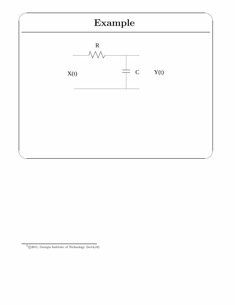
Example

R

CX(t) Y(t)

0 c2011, Georgia Institute of Technology (lect4 18)

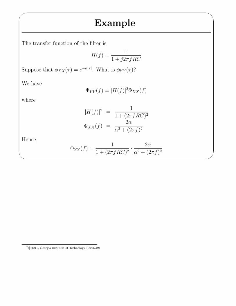
Example

The transfer function of the filter is

H(f) =1

1 + j2fRC

Suppose that XX() = e| |. What is Y Y ()?

We haveY Y (f) = |H(f)|

2XX(f)

where

|H(f)|2 =1

1 + (2fRC)2

XX(f) =2

2 + (2f)2

Hence,

Y Y (f) =1

1 + (2fRC)2

2

2 + (2f)2

0 c2011, Georgia Institute of Technology (lect4 19)

Example

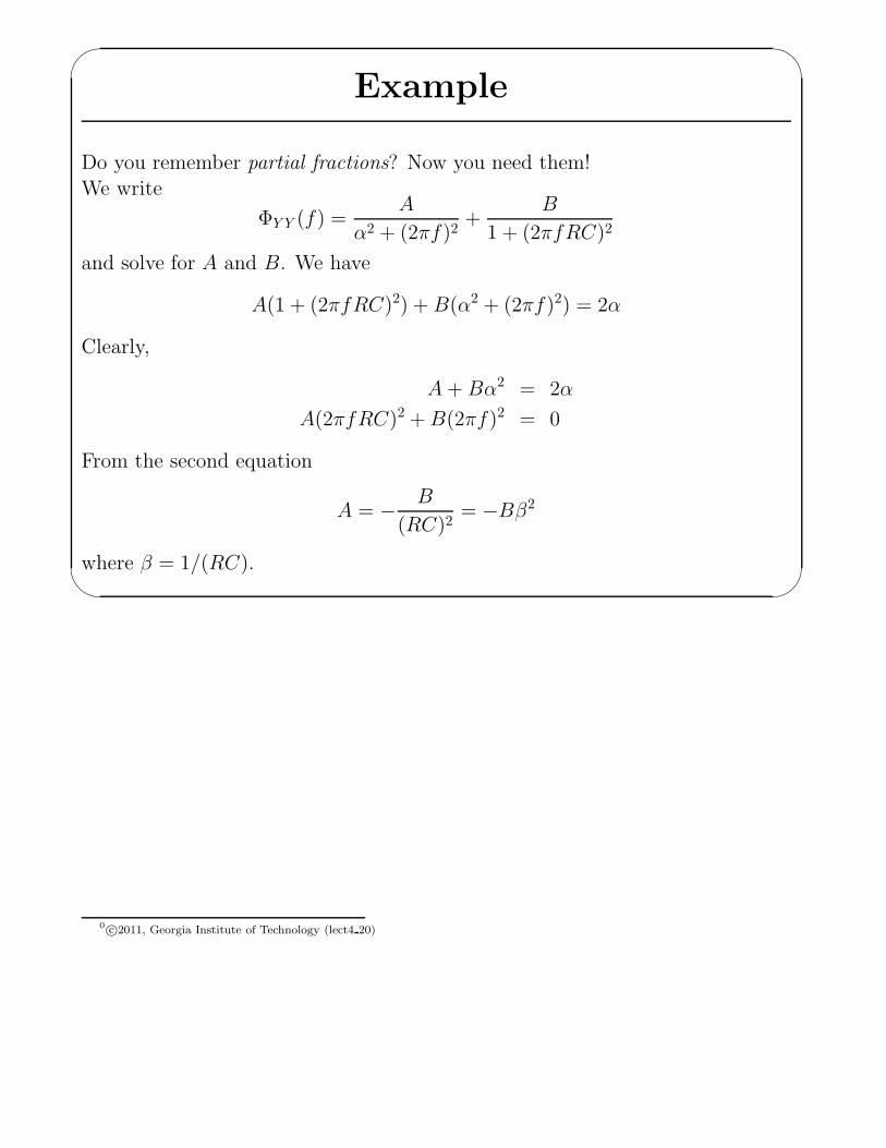
Do you remember partial fractions? Now you need them!We write

Y Y (f) =A

2 + (2f)2+

B

1 + (2fRC)2

and solve for A and B. We have

A(1 + (2fRC)2) + B(2 + (2f)2) = 2

Clearly,

A+ B2 = 2

A(2fRC)2 +B(2f)2 = 0

From the second equation

A = B

(RC)2= B2

where = 1/(RC).

0 c2011, Georgia Institute of Technology (lect4 20)

Example

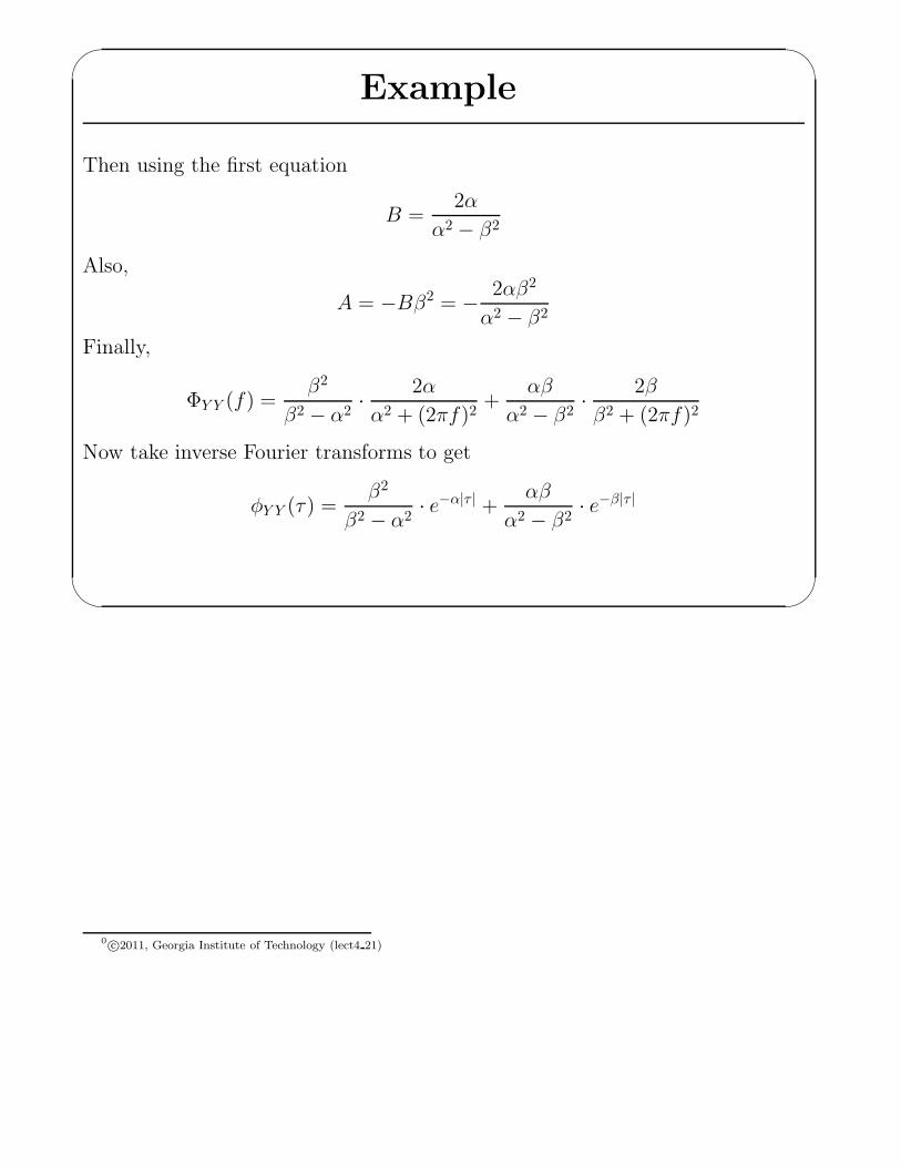
Then using the first equation

B =2

2 2

Also,

A = B2 = 22

2 2

Finally,

Y Y (f) =2

2 2

2

2 + (2f)2+

2 2

2

2 + (2f)2

Now take inverse Fourier transforms to get

Y Y () =2

2 2 e| | +

2 2 e| |

0 c2011, Georgia Institute of Technology (lect4 21)

Discrete-time Random Processes

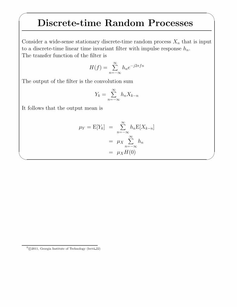
Consider a wide-sense stationary discrete-time random process Xn that is inputto a discrete-time linear time invariant filter with impulse response hn.The transfer function of the filter is

H(f) =

n=hne

j2fn

The output of the filter is the convolution sum

Yk =

n=hnXkn

It follows that the output mean is

Y = E[Yk] =

n=hnE[Xkn]

= X

n=hn

= XH(0)

0 c2011, Georgia Institute of Technology (lect4 22)

Discrete-time Random Processes

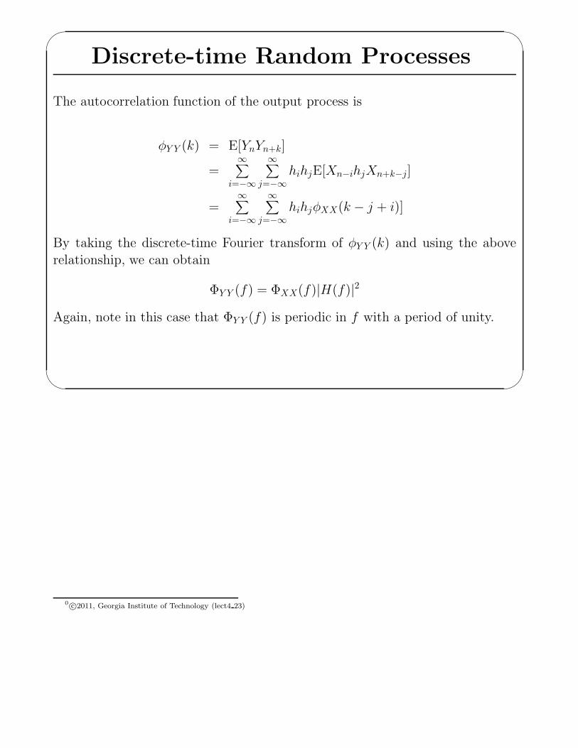
The autocorrelation function of the output process is

Y Y (k) = E[YnYn+k]

=

i=

j=

hihjE[XnihjXn+kj]

=

i=

j=

hihjXX(k j + i)]

By taking the discrete-time Fourier transform of Y Y (k) and using the above

relationship, we can obtain

Y Y (f) = XX(f)|H(f)|2