The views expressed in this report are solely those of the author.No responsibility for them should be attributed to the Bank of Canada.

November 1994

WEALTH, DISPOSABLE INCOMEAND CONSUMPTION:

Some Evidence for Canada

byR. Tiff Macklem

0713–7931ISBN 0-662-22503-1

Printed in Canada on recycled paper

CONTENTS

ACKNOWLEDGMENTS ......................................................................................v

ABSTRACT ......................................................................................................... vii

RÉSUMÉ ............................................................................................................ viii

1 INTRODUCTION ............................................................................................1

2 MEASURING WEALTH .................................................................................5

2.1 Human wealth .........................................................................................6

2.1.1 A time series model for net income and

the real interest rate ......................................................................7

2.2 Computing the cumulative growth factors ............................................12

2.3 Non-human wealth ................................................................................18

3 IS WEALTH USEFUL IN EXPLAINING CONSUMPTION? .....................23

3.1 Long-run analysis ..................................................................................24

3.2 Dynamic consumption functions ...........................................................32

4 CONCLUSION ...............................................................................................45

APPENDIX 1: The data.......................................................................................47

APPENDIX 2: Closed-form solution for the cumulative

growth factors ............................................................................57

APPENDIX 3: Wealth and its components

(per capita in constant 1986 dollars)...........................................59

BIBLIOGRAPHY .................................................................................................63

v

ACKNOWLEDGMENTS

I am grateful for many helpful suggestions and comments from mycolleagues at the Bank of Canada, particularly Robert Amano,Jean-François Fillion, Doug Hostland, Steve Poloz and David Rose. I amalso grateful for useful suggestions from participants of the 1993 Meetingsof the Canadian Economics Association especially Charles Beach andHuntley Schaller, and for valuable assistance from Chris Lavigne andPhillipe Karam. I gratefully acknowledge the use of Bruce Hansen’s Gausscode for his structural stability tests for I(1) processes, and the use ofsubroutines programmed in RATS by Simon van Norden and RobertAmano, subroutines that perform cointegration and unit root tests, rollingChow tests, recursive estimation and residual-based diagnostic tests. Anyerrors or omissions are solely my responsibility.

vii

ABSTRACT

The author develops a measure of aggregate private sector wealth inCanada and examines its ability to explain aggregate consumption of non-durables and services. This wealth measure includes financial, physicaland human wealth.

The author measures human wealth as the expected present valueof aggregate labour income, net of government expenditures, based on adiscrete state-space approximation of an estimated bivariate vector autore-gression for the real interest rate and the growth rate of labour income, netof government expenditures. His general approach to measuring financialand physical (non-human) wealth is to consolidate the assets and liabilitiesof the various sectors of the economy so as to measure the net worth of theultimate owners of private-sector wealth – households. To the extent possi-ble, the author measures non-human wealth at market value.

The relationship between consumption and wealth is explored as ameans both of gauging the usefulness of the wealth measures developed inthis report and of improving on empirical consumption models forCanada. The principal empirical finding is that both wealth and disposableincome are important determinants of consumption. Including wealth inthe consumption function is particularly helpful in explaining the con-sumption boom of the late 1980s.

viii

RÉSUMÉ

Dans le présent rapport, l’auteur élabore une mesure de la richesse globaledu secteur privé au Canada et examine sa capacité d’expliquer la consom-mation globale de biens non durables et de services. Cette mesure englobela richesse financière, la richesse physique et la richesse humaine.

L’auteur définit la richesse humaine comme la valeur actuelle antici-pée du revenu global du travail, nette des dépenses publiques. Cettemesure est basée sur une approximation discrète d’espace-état d’une auto-régression vectorielle à deux variables, estimée pour le taux d’intérêt réelet le taux de croissance du revenu du travail net des dépenses publiques.L’approche générale utilisée par l’auteur pour mesurer la richesse finan-cière et la richesse physique (non humaine) consiste à regrouper l’actif et lepassif des divers secteurs de l’économie de façon à obtenir une estimationde la situation nette des détenteurs ultimes de la richesse du secteur privé,à savoir les ménages. Dans la mesure du possible, l’auteur mesure larichesse non humaine à la valeur du marché.

L’auteur cherche à déterminer la relation entre la consommation etla richesse afin de pouvoir évaluer l’utilité des mesures de la richesse éla-borées dans le présent rapport et d’améliorer les modèles empiriques deconsommation au Canada. Le principal résultat empirique auquel il par-vient est que tant la richesse que le revenu disponible constituent desdéterminants importants de la consommation. L’inclusion de la richessedans la fonction de consommation est particulièrement utile pour expli-quer l’essor de la consommation à la fin des années 80.

1

1 INTRODUCTION

Empirical research on consumption behaviour over the past 15 or so yearshas been strongly influenced by two papers, both published in 1978. Hall(1978) examined the stochastic implications of the permanent incomehypothesis, and Davidson et al. (1978) developed dynamic econometricmodels for aggregate consumption based on an error-correction (EC)specification.

Hall’s innovation was to exploit the restrictions implied by the first-order conditions of a representative consumer’s intertemporal optimiza-tion problem. The attractive feature of this approach is that the resultingEuler equations do not require the specification of all future variables rele-vant to the household’s consumption decisions, so the difficulties associ-ated with measuring wealth and obtaining closed-form relationshipsbetween consumption and wealth can be largely avoided.

These advantages are, however, achieved at some cost. While theestimation of Euler equations allows the empirical researcher to examinewhether consumers adjust optimally between adjacent periods, it provideslittle direct evidence on the determinants of consumption or on how vari-ous random disturbances or policy changes are transmitted to consump-tion. Consequently, the Euler equation approach to modellingconsumption is not particularly well-suited to policy analysis and forecast-ing. In addition, the stochastic permanent income model also suffers thepractical problem that it is frequently rejected by the data (see, for example,Flavin 1981, Hayashi 1982, Nelson 1987, and Wirjanto 1991). These rejec-tions are often interpreted as evidence that some consumers face bindingliquidity constraints (see Hall and Mishkin 1982, Flavin 1985, Zeldes 1989,and Campbell and Mankiw 1990).

Partly as a result of these limitations, policy makers and practition-ers in general have largely turned to the more eclectic EC consumptionmodel proposed by Davidson et al. (1978). The EC model is not usuallyderived from the micro foundations of optimizing behaviour, but is pro-posed as a robust empirical relationship between macro aggregates that is

2

formulated using both the cointegration analysis of Engle and Granger(1987) and the principles of dynamic econometric modelling as outlined inHendry and Richard (1982). Error-correction consumption models havebeen estimated for a wide range of countries – see Davidson et al. (1978)and Davidson and Hendry (1981) for the United Kingdom, Harnett (1988)for the United States, Sawyer (1991) for Canada, Rossi and Schiantarelli(1982) for Italy, Steel (1987) for Belgium, and Thury (1989) for Austria.

The standard EC model follows a long tradition in macroeconomicsof specifying a static or long-run relationship between consumption anddisposable income, and then augments this long-run consumption func-tion with additional variables aimed at explaining short-run deviationsfrom the long-run trend. Some researchers have also included the realinterest rate in the long-run consumption function (see Davidson andHendry 1981 and Sawyer 1991), in part to capture wealth effects. Measuresof liquid assets have also been included (Hendry and von Ungern-Sternberg 1981 and Patterson 1991) for the same reason. To a large degree,however, EC models have ignored the implication of the life cycle-permanent income hypothesis that consumption is determined by wealthor its flow equivalent, permanent income. This report attempts to redressthis situation.

This report has two main goals: to develop a measure of aggregateprivate sector wealth in Canada that includes financial, physical andhuman wealth, and to examine the ability of this wealth measure to explainaggregate consumption. The relationship between consumption andwealth is explored both as a means of gauging the usefulness of the wealthmeasures developed in this report and to improve upon empirical con-sumption models for Canada. By augmenting the standard EC consump-tion model with a comprehensive measure of wealth, this study goes partway towards bridging the gap between life cycle–permanent income con-sumption equations, and the more empirically motivated EC consumptionmodels based on disposable income.

Many important economic questions are connected with the behav-iour of wealth. These include the effects of tax policies on savings, the

3

impact of fluctuations in the prices of equity, bonds and housing on aggre-gate demand, and the consequences of changes in the level of foreignindebtedness. Comprehensive measures of wealth that include bothhuman and non-human wealth have been previously constructed forCanada at an annual frequency by Irvine (1980) and Beach, Boadway andBruce (1988). The more recent Beach, Boadway and Bruce study providesannual estimates of human and non-human wealth from 1964 to 1981 foreach of 10 age groups. Human wealth is constructed by taking the presentvalue of the projected after-tax earnings of each age group based on a timetrend and their life-cycle earnings profile. Non-human wealth is con-structed as the sum of the capitalized flow of capital income and the accu-mulated present value of tax-sheltered savings. Aggregate human wealthand non-human wealth are obtained by summing across age cohorts.

At a minimum, the current study provides alternative measures ofhuman and non-human wealth that extend from 1963 through to 1993 at aquarterly frequency. Relative to the earlier work by Irvine and Beach,Boadway and Bruce, the construction of human wealth takes a more aggre-gated approach, which allows for greater recognition of the joint statisticalproperties of innovations in income and interest rates. Human wealth iscomputed as the expected present value of aggregate labour income net ofgovernment expenditures based on an estimated bivariate vector autore-gression (VAR) for the real interest rate and the growth rate of labourincome net of government expenditures. Owing to the non-linear nature ofthe present-value formula, the estimated VAR is approximated as a dis-crete-value finite-state Markov chain, thereby permitting expectations tobe computed as a weighted sum over possible outcomes instead of as anintractable integral. Non-human wealth in the current study is based onactual stock data obtained largely from the national balance sheet accountsand adjusted to obtain market values, rather than on cumulated capitaland savings flows, as in Beach, Boadway and Bruce.

The ability of the new wealth measures to explain consumption isexplored in the context of a general consumption equation that includes

4

both disposable income and wealth. Implicit in this approach is the pre-sumption that the stock of wealth is exogenous to the portfolio-allocationproblem so that the composition of wealth does not influence the con-sumption-savings decision.1 The empirical analysis begins by examiningthe long-run relationship between consumption, wealth and disposableincome using standard tests for cointegration, and provides asymptoticallyefficient estimates of the long-run propensities to consume out of wealthand disposable income using two alternative estimation procedures. Thislong-run analysis is complemented by estimating dynamic EC models forconsumption that include wealth.

The principal finding is that wealth is a significant determinant ofconsumption, particularly in the long run, but disposable income contin-ues to exert an important influence on consumption in both the short runand the long run. The influence of disposable income may be interpreted asevidence of liquidity constraints, but it could also be proxying in part forwealth itself. There is also some evidence that consumption responds dif-ferently to different components of wealth. This may reflect the differentstochastic behaviour of alternative assets, the importance of consumer het-erogeneity, or the absence of separability between the portfolio-allocationand consumption-savings decisions.

1. The alternative is to model the portfolio-allocation and consumption-savings decisionsin an integrated framework as in Poloz (1986).

5

2 MEASURING WEALTH

In a competitive economy with perfect capital markets the representativeconsumer’s wealth is the sum of his financial and physical assets net of lia-bilities (non-human wealth) plus the expected discounted value of his cur-rent and expected future after-tax labour income (human wealth). In anopen economy, non-human wealth will generally include both domesticand foreign assets net of liabilities. Summing across consumers and divid-ing by the population yields aggregate per capita real wealth. If we defineall aggregate variables in real per capita terms, real per capita wealth (W)

can be written as:

(2.1)

where A is net domestic and foreign physical and financial assets, isdomestic holdings of government debt, L is labour income, T is taxes net oftransfers, r is the real interest (or discount) rate, and is the expectationsoperator conditioned on information available at time t.

If we add the assumptions of intergenerational altruism and lumpsum taxes, wealth is characterized by the well-known Ricardian equiva-lence proposition. For a given path for government expenditures and theforeign debt, wealth is invariant to the timing of taxes and the size of thegovernment debt. Domestically held government debt nets out of wealth,since rational consumers realize that the value of the government debt theyhold is offset by future tax liabilities. This can be demonstrated by combin-ing (2.1) with the government’s budget constraint. The government’s life-time budget constraint requires that the present value of taxes is sufficientto pay for the present value of government expenditures plus any out-standing government debt:

Wt At Dtd

Lt Tt–( ) Et1

1 r t j++--------------------

Lt i+ Tt i+–( )j 1=

i

∏i 1=

∞

∑+ + +=

Dd

Et

6

(2.2)

where G is real government expenditures on goods and services and isthe government debt held by foreigners. Substituting (2.2) into (2.1) yieldsaggregate wealth as a function of government expenditures and foreignholdings of government debt:

(2.3)

The measurement of wealth developed in this study adopts the def-inition of wealth given in (2.3). While (2.1) and (2.3) are equivalent, (2.3)provides a more convenient basis for measurement because it allows us toignore difficult issues regarding the timing of future taxes and deficits.Wealth depends on real government expenditures and not on how they arefinanced.2

2.1 Human wealth

According to the definition of wealth given in (2.3), human wealth is thepresent discounted value of current and future labour income net of gov-ernment expenditures. If we let and denote its growth rate by x,human wealth can be written as the product of current labour income netof government expenditures, and a term that captures the effects ofexpected future growth:

2. Admittedly, this representation of wealth does not address several real-world features.In particular, consumers and governments typically cannot borrow at the same interestrates, taxes are not lump sum, and some consumers may have finite horizons. The test willbe whether (2.3) provides an empirically useful measure of wealth.

Tt Et1

1 r t j++--------------------

Tt i+j 1=

i

∏i 1=

∞

∑+

= Dtd

Dtf

Gt Et1

1 r t j++--------------------

Gt i+j 1=

i

∏i 1=

∞

∑+ + +

Df

Wt At Dtf

– Lt Gt–( )+=

E+ t1

1 r t j++--------------------

Lt i+ Gt i+–( )j 1=

i

∏i 1=

∞

∑

X L G–=

7

(2.4)

where H is human wealth and represents the term in the outer squarebrackets. The problematic aspect of measuring human wealth is that thecumulative growth factor is not directly observable, because it dependson expectations.

One approach to measuring would be to develop a fully articu-lated macro model and then invoke the rational expectations hypothesis.This approach would be very ambitious. A more modest approach, and theone pursued in this study, is to model the behaviour of variables overwhich expectations must be taken using time-series techniques and thenuse the resulting time-series model to compute expectations of the future.This approach is implemented by estimating a bivariate VAR to character-ize the joint distribution of the growth rate of labour income net of govern-ment expenditures (hereafter, net income) and the real interest rate. Theestimated bivariate VAR is then approximated as a discrete-valued finite-state vector Markov chain and this approximated system is used to com-pute the expected discounted value of future net income growth.

2.1.1 A time series model for net income and the real interest rate

The first step is to define net income and the interest rate and to examinetheir time-series properties. All the variables used in this study togetherwith the raw data sources are described in Appendix 1, but the mostimportant details deserve some comment.

In an effort to get a more complete measure of aggregate labourincome, the published labour income series is augmented to include labourincome in the farming and unincorporated business sectors. It is assumedthat the share of labour in these two categories is the same as for the overalleconomy.

Government expenditure on goods and services is measured as thereported quarterly government expenditure series less the fraction of the

Ht Xt 1 Et

1 xt j++

1 r t j++--------------------

j 1=

i

∏i 1=

∞

∑+ XtΓt≡=

Γ

Γ

Γ

8

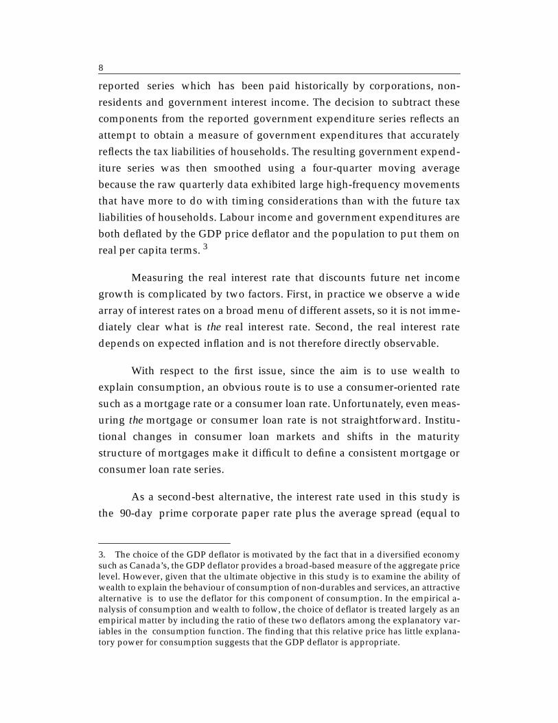
reported series which has been paid historically by corporations, non-residents and government interest income. The decision to subtract thesecomponents from the reported government expenditure series reflects anattempt to obtain a measure of government expenditures that accuratelyreflects the tax liabilities of households. The resulting government expend-iture series was then smoothed using a four-quarter moving averagebecause the raw quarterly data exhibited large high-frequency movementsthat have more to do with timing considerations than with the future taxliabilities of households. Labour income and government expenditures areboth deflated by the GDP price deflator and the population to put them onreal per capita terms. 3

Measuring the real interest rate that discounts future net incomegrowth is complicated by two factors. First, in practice we observe a widearray of interest rates on a broad menu of different assets, so it is not imme-diately clear what is the real interest rate. Second, the real interest ratedepends on expected inflation and is not therefore directly observable.

With respect to the first issue, since the aim is to use wealth toexplain consumption, an obvious route is to use a consumer-oriented ratesuch as a mortgage rate or a consumer loan rate. Unfortunately, even meas-uring the mortgage or consumer loan rate is not straightforward. Institu-tional changes in consumer loan markets and shifts in the maturitystructure of mortgages make it difficult to define a consistent mortgage orconsumer loan rate series.

As a second-best alternative, the interest rate used in this study isthe 90-day prime corporate paper rate plus the average spread (equal to

3. The choice of the GDP deflator is motivated by the fact that in a diversified economysuch as Canada’s, the GDP deflator provides a broad-based measure of the aggregate pricelevel. However, given that the ultimate objective in this study is to examine the ability ofwealth to explain the behaviour of consumption of non-durables and services, an attractivealternative is to use the deflator for this component of consumption. In the empirical a-nalysis of consumption and wealth to follow, the choice of deflator is treated largely as anempirical matter by including the ratio of these two deflators among the explanatory var-iables in the consumption function. The finding that this relative price has little explana-tory power for consumption suggests that the GDP deflator is appropriate.

9

2.3 percentage points) between the mortgage rate and the prime corporatepaper rate. This nominal interest rate is converted to a real rate by subtract-ing expected inflation. Consistent with the measurement of real incomeand the other components of wealth, inflation itself is measured using theGDP deflator. Expected inflation is proxied by a two-period moving aver-age of past inflation. This proxy is motivated by the fact that, over the sam-ple in question, GDP inflation is well-described by a second-orderautoregressive, AR(2), process with approximately equal coefficients thatsum to unity.4

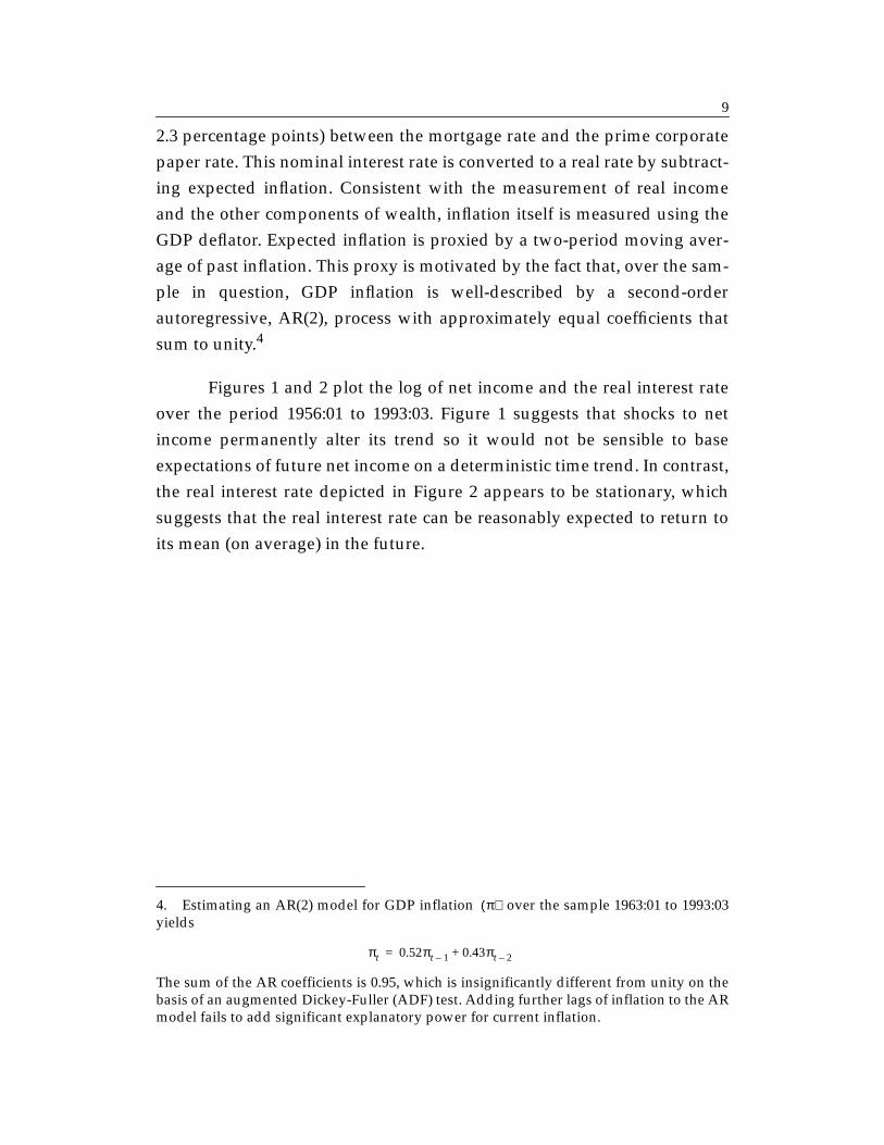
Figures 1 and 2 plot the log of net income and the real interest rateover the period 1956:01 to 1993:03. Figure 1 suggests that shocks to netincome permanently alter its trend so it would not be sensible to baseexpectations of future net income on a deterministic time trend. In contrast,the real interest rate depicted in Figure 2 appears to be stationary, whichsuggests that the real interest rate can be reasonably expected to return toits mean (on average) in the future.

4. Estimating an AR(2) model for GDP inflation over the sample 1963:01 to 1993:03yields

The sum of the AR coefficients is 0.95, which is insignificantly different from unity on thebasis of an augmented Dickey-Fuller (ADF) test. Adding further lags of inflation to the ARmodel fails to add significant explanatory power for current inflation.

π( )

πt 0.52πt 1– 0.43πt 2–+=

10

1960 1965 1970 1975 1980 1985 19907.3

7.4

7.5

7.6

7.7

7.8

7.9

8.0

8.1

Figure 1Real per capita labour income net

of government expenditures(in logs; quarterly rates)

1960 1965 1970 1975 1980 1985 1990–0.01

0.00

0.01

0.02

0.03

0.04

Figure 2The real interest rate

(quarterly rates)

11

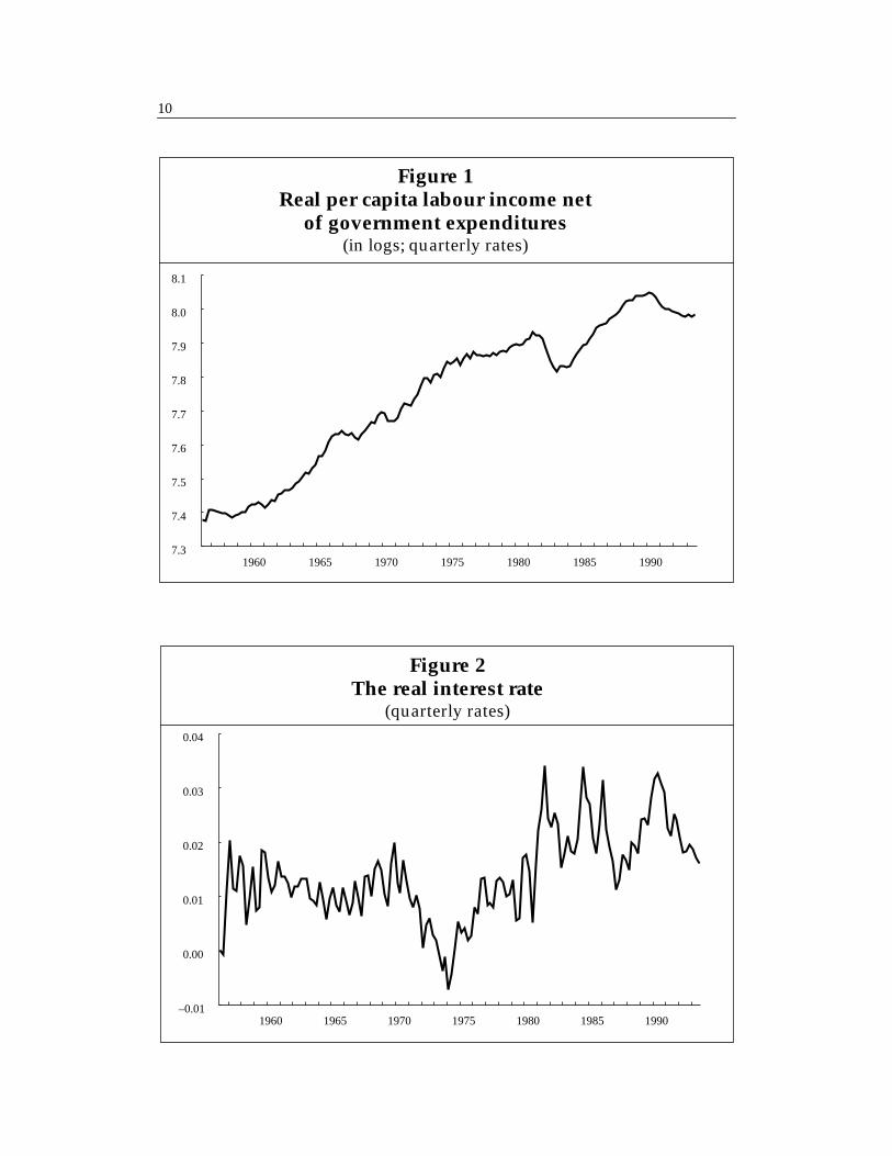
The time-series properties of net income and the real interest rateare investigated more formally using two popular tests for unit roots – theADF test advocated by Dickey and Fuller (1979) and Said and Dickey(1984), and the non-parametric test proposed by Phillips and Perron (1988).The test results are reported in Table 1 and are largely consistent with theinferences made on the basis of Figures 1 and 2. The ADF test and thePhillips-Perron (PP) test both fail to reject the null of a unit root in the logof net income but convincingly reject this null in the case of its first differ-ence. This suggests that the trend in net income is indeed stochastic andthat the growth rate of net income is a stationary process.

Table 1Tests for unit roots –

augmented Dickey-Fuller (ADF) andPhillips-Perron (PP) tests

Sample: 1956:03–1993:03

Variables ADF lagsADF

t–ratioPP

t–ratio5%

critical

log of net income 3 –1.66 –2.21 –3.43

log of net income 1 –6.45 –11.22 –3.43

real interest rate 2 –2.52 –5.32 –3.43

Note: All tests are conducted with a time trend included in the unit-root re-gression. In the case of the ADF test, the number of lagged first differ-ences of the dependent variable to include on the right-hand side waschosen following the selection procedure advocated by Hall (1989).This involves sequentially reducing the number of lags included untilthe t-statistic on the highest-order lag included is significantly differentfrom zero. The lag selection began with four lags and used a 10 per centlevel for the t-test. For the PP test, the number of lags used in the non-parametric correction for serial dependence is set to the square root ofthe number of observations used, following the suggestion of Andrews(1991). The critical values for the ADF and PP statistics are the sameand are computed for the actual number of observations available,based on the response surface estimates given in MacKinnon (1991).

∆

12

In the case of the real interest rate, the evidence is not as clear, but onbalance it appears to favour stationarity. The more powerful PP test rejectsthe null of a unit root at the 5 per cent level, while the reported ADF t-ratiodoes not. However, the ADF test in this case is very sensitive to the numberof lagged first differences that are included in the regression. Based onHall’s (1989) selection procedure, two lags were included yielding an ADFt-ratio of –2.54.5 When only one lag is included, the ADF t-ratio fallsto –4.12, which then rejects the null of a unit root at the 5 per cent level.

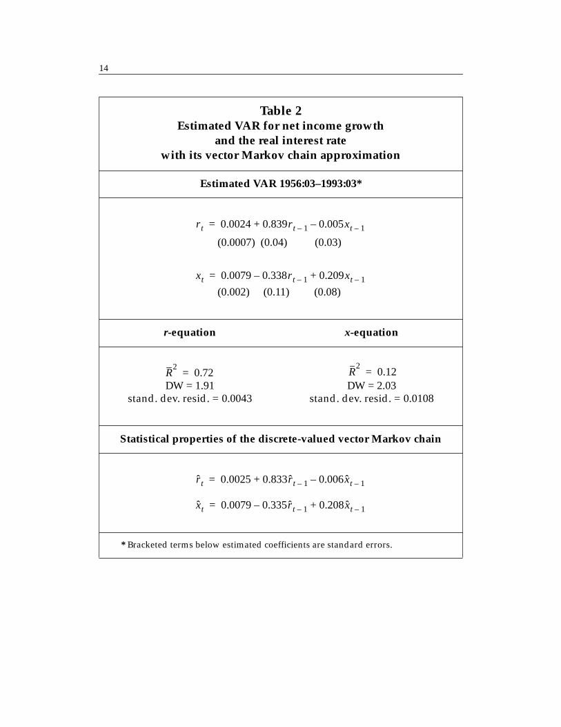
The joint distribution of net income growth and the real interest rateis estimated using a VAR. Owing to computational constraints associatedwith the finite-state Markov chain approximation to be discussed below,the VAR is restricted to be of first order. Fortunately, this constraint doesnot appear to be too serious, since the first-order model captures most ofthe predictive content of past income growth and real interest rates. Theestimated VAR together with some basic diagnostics are reported in thetop panel of Table 2. Both net income growth and the real interest rateexhibit positive persistence, with the interest rate being the more seriallydependent of the two. The coefficient on the lagged real interest rate in thenet income growth equation is significantly negative, consistent with theconventional view that raising real interest rates dampens economicactivity.

2.2 Computing the cumulative growth factors

The VAR can be used to forecast net income growth and the real interestrate, thereby providing an estimate of their expected future path. This,however, is not sufficient for the measurement of human wealth, since thecumulative growth factor is a non-linear function of net income growthand the real interest rate. The expected value of a non-linear function is notthe function of the expectation, so we cannot simply replace andin (2.4) with their j-period ahead forecasts from the VAR and then drop the

5. See the notes accompanying Table 1 for a short description of Hall’s (1989) lag-lengthselection procedure.

Γ

xt j+ r t j+

13

expectation operator. Instead, the expectation in (2.4) must be evaluateddirectly.

This is accomplished by approximating the continuous-valued VARas a discrete-valued finite-state vector Markov chain. If net income growth,the real interest rate and their joint distribution are made to be discrete,expectations may be solved as a probability weighted sum rather than asan intractable integral. The approximation procedure is due to Tauchen(1986) and it is implemented by means of 25-point grids for net incomegrowth and the real interest rate. The finite-state system therefore has

states, and the transition matrix describing the dynamics of thesystem is . The statistical properties of the discrete-valued systemare summarized in the bottom panel of Table 2. The circumflex on anddistinguishes the series of discrete values from the true series of continu-ous values. From a comparison of the upper and lower panels of Table 2, itis apparent that the finite-state vector Markov chain closely mimics the sta-tistical properties of the VAR.

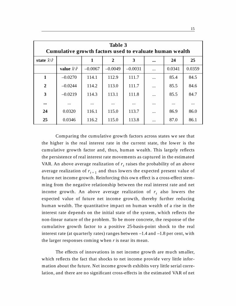
With the approximated system, the cumulative growth factors canbe computed directly for every state of the system. The explicit solution for

is given in Appendix 2, and a sample of the results is provided in Table 3.The values for and in the second column and row respectively are thediscrete values that net income growth and the real interest rate (bothmeasured at quarterly rates) can take on. For example, suppose, is instate 3 and is in state 24. The net income growth is –2.19 per cent at quar-terly rates, the discount rate is 3.41 per cent at quarterly rates, and thecumulative growth factor is 85.5. If the level of net income was, say,$3,000 at quarterly rates, then real per capita human wealth would be$3,000 x 85.5 = $256,500.

252

625=

625 625×x r

Γ

Γx r

x

r

14

Table 2Estimated VAR for net income growth

and the real interest ratewith its vector Markov chain approximation

Estimated VAR 1956:03–1993:03*

(0.0007) (0.04) (0.03)

(0.002) (0.11) (0.08)

r-equation x-equation

DW = 1.91stand. dev. resid. = 0.0043

DW = 2.03stand. dev. resid. = 0.0108

Statistical properties of the discrete-valued vector Markov chain

* Bracketed terms below estimated coefficients are standard errors.

r t 0.0024 0.839r t 1– 0.005xt 1––+=

xt 0.0079 0.338r t 1– 0.209xt 1–+–=

R2

0.72= R2

0.12=

r t 0.0025 0.833r t 1– 0.006xt 1––+=

xt 0.0079 0.335r t 1– 0.208xt 1–+–=

15

Comparing the cumulative growth factors across states we see thatthe higher is the real interest rate in the current state, the lower is thecumulative growth factor and, thus, human wealth. This largely reflectsthe persistence of real interest rate movements as captured in the estimatedVAR. An above average realization of raises the probability of an aboveaverage realization of and thus lowers the expected present value offuture net income growth. Reinforcing this own effect is a cross-effect stem-ming from the negative relationship between the real interest rate and netincome growth. An above average realization of also lowers theexpected value of future net income growth, thereby further reducinghuman wealth. The quantitative impact on human wealth of a rise in theinterest rate depends on the initial state of the system, which reflects thenon-linear nature of the problem. To be more concrete, the response of thecumulative growth factor to a positive 25-basis-point shock to the realinterest rate (at quarterly rates) ranges between –1.4 and –1.8 per cent, withthe larger responses coming when r is near its mean.

The effects of innovations in net income growth are much smaller,which reflects the fact that shocks to net income provide very little infor-mation about the future. Net income growth exhibits very little serial corre-lation, and there are no significant cross-effects in the estimated VAR of net

Table 3Cumulative growth factors used to evaluate human wealth

state 1 2 3 ... 24 25

value –0.0067 –0.0049 –0.0031 ... 0.0341 0.0359

1 –0.0270 114.1 112.9 111.7 ... 85.4 84.5

2 –0.0244 114.2 113.0 111.7 ... 85.5 84.6

3 –0.0219 114.3 113.1 111.8 ... 85.5 84.7

... ... ... ... ... ... ... ...

24 0.0320 116.1 115.0 113.7 ... 86.9 86.0

25 0.0346 116.2 115.0 113.8 ... 87.0 86.1

x\ r

x\ r

r t

r t 1+

r t

16

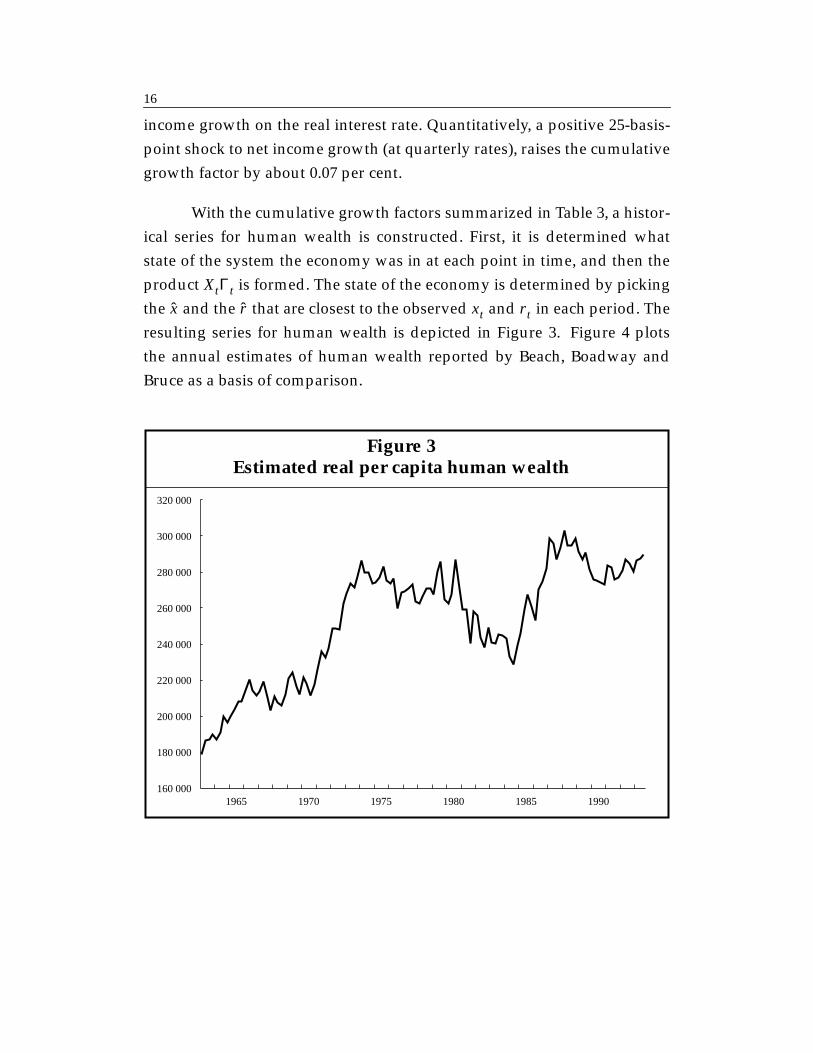
income growth on the real interest rate. Quantitatively, a positive 25-basis-point shock to net income growth (at quarterly rates), raises the cumulativegrowth factor by about 0.07 per cent.

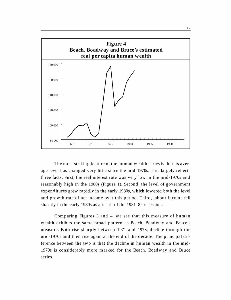
With the cumulative growth factors summarized in Table 3, a histor-ical series for human wealth is constructed. First, it is determined whatstate of the system the economy was in at each point in time, and then theproduct is formed. The state of the economy is determined by pickingthe and the that are closest to the observed and in each period. Theresulting series for human wealth is depicted in Figure 3. Figure 4 plotsthe annual estimates of human wealth reported by Beach, Boadway andBruce as a basis of comparison.

XtΓt

x r xt r t

Figure 3Estimated real per capita human wealth

1965 1970 1975 1980 1985 1990160 000

180 000

200 000

220 000

240 000

260 000

280 000

300 000

320 000

17

The most striking feature of the human wealth series is that its aver-age level has changed very little since the mid-1970s. This largely reflectsthree facts. First, the real interest rate was very low in the mid-1970s andreasonably high in the 1980s (Figure 1). Second, the level of governmentexpenditures grew rapidly in the early 1980s, which lowered both the leveland growth rate of net income over this period. Third, labour income fellsharply in the early 1980s as a result of the 1981–82 recession.

Comparing Figures 3 and 4, we see that this measure of humanwealth exhibits the same broad pattern as Beach, Boadway and Bruce’smeasure. Both rise sharply between 1971 and 1973, decline through themid-1970s and then rise again at the end of the decade. The principal dif-ference between the two is that the decline in human wealth in the mid-1970s is considerably more marked for the Beach, Boadway and Bruceseries.

1965 1970 1975 1980 1985 199080 000

100 000

120 000

140 000

160 000

180 000

Figure 4Beach, Boadway and Bruce’s estimated

real per capita human wealth

18

In the second half of the 1980s human wealth grew very rapidlyowing to the combination of strong growth in net income (Figure 1) andfalling real interest rates (Figure 2). This growth slowed as the decadeended and reversed somewhat in the 1990–91 recession.

2.3 Non-human wealth

In principle, measuring non-human wealth is relatively straightforward.The main task is to assemble the data and in some cases make adjustmentsto obtain market-value measures. The general approach to measuring non-human wealth is to consolidate carefully the assets and liabilities of thevarious sectors of the economy in an effort to “see through” the financialstructure of the economy and to measure only the net worth of the ultimateowners of private-sector wealth – households. This “balance sheet”approach is implemented using quarterly national accounts data and bycombining annual data from the national balance sheet accounts withquarterly data from the financial flow accounts. Unfortunately, the annualstock data and the quarterly flow data do not match up in the sense thatyear-to-year changes in the stock do not equal the sum of the flows overthe year, so an adjustment was made to reconcile the stock-flow series.6

From these consistent stock-flow data, the components of non-humanwealth are constructed on a real per capita basis through division by theGDP price deflator and the population. The construction of these variablesis described in detail in Appendix 1, but an overview is provided below.

Government debt held by foreigners is the sum of treasurybills and federal, provincial and municipal government bonds held bynon-residents. Net domestic and foreign assets are defined to be thesum of non-financial and financial assets held by persons and unincorpo-rated businesses, less the liabilities of this sector, plus the value of theCanada and Quebec Pension plans, and less the value of domestically heldoutstanding government debt. Non-financial assets include residential and

6. More specifically, the difference between the four-quarter cumulated flow and theyear-end stock is allocated to each of the four quarters in proportion to the size of the flowin each quarter.

Dtf( )

A( )

19

non-residential structures, machinery and equipment, consumer durables,inventories and land. Financial assets are defined as the sum of currencyand deposits, corporate bonds, life insurance and pensions, foreign invest-ments and equity. The principal liabilities of persons and unincorporatedbusinesses are consumer and mortgage loans and other loans.

To understand the construction of net assets, it is important to dis-tinguish between the components of and their sum. This point is wellillustrated by the treatment of deposits and government debt. Deposits area component of , which implies that this variable includes inside money.This, however, should not be the case, since inside money should be offsetby consumer and business loans. Consumer and business loans are a liabil-ity to consumers, either directly or indirectly through their equity holdingsin firms. In the case of government debt, includes the government debtheld directly by persons and unincorporated businesses, and then sub-tracts the total outstanding stock of domestically held government debt. Asa result, both the government debt held directly by households and thegovernment debt held by firms (and thus indirectly by households throughtheir equity holdings) net out.

In the case of the three largest components of non-human wealth,adjustments are made to improve the quality of the market valuation ofthese assets. Equity in the national balance sheet accounts is measured at“current” value, which is defined as the sum of book value and cumulatedretained earnings. To obtain a market-value measure, the current value ofequity reported in the national balance sheet accounts is replaced with ameasure of the book value of equity that is scaled by the growth rate of theTSE 300 composite stock price index. Bonds are reported in the nationalbalance sheet accounts at book value. In the case of treasury bills, this is nota serious problem, since book and market values do not differ substantiallyfor these short-term bonds. In the case of federal, provincial and municipalbonds with a longer term to maturity, the book value series reported in thenational balance sheet accounts is replaced with a market value serieswhich is constructed by multiplying the original book value series by amarket price index that is constructed using Rose and Selody’s (1985)

A

A

A

20

present-value model. In the case of corporate bonds, no comparable mar-ket adjustment was made, since holdings of corporate bonds by personsand unincorporated businesses is relatively small. Housing is measured atmarket value by multiplying the constant dollar stock of housing by themultiple listings housing price index.

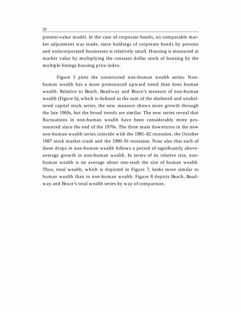
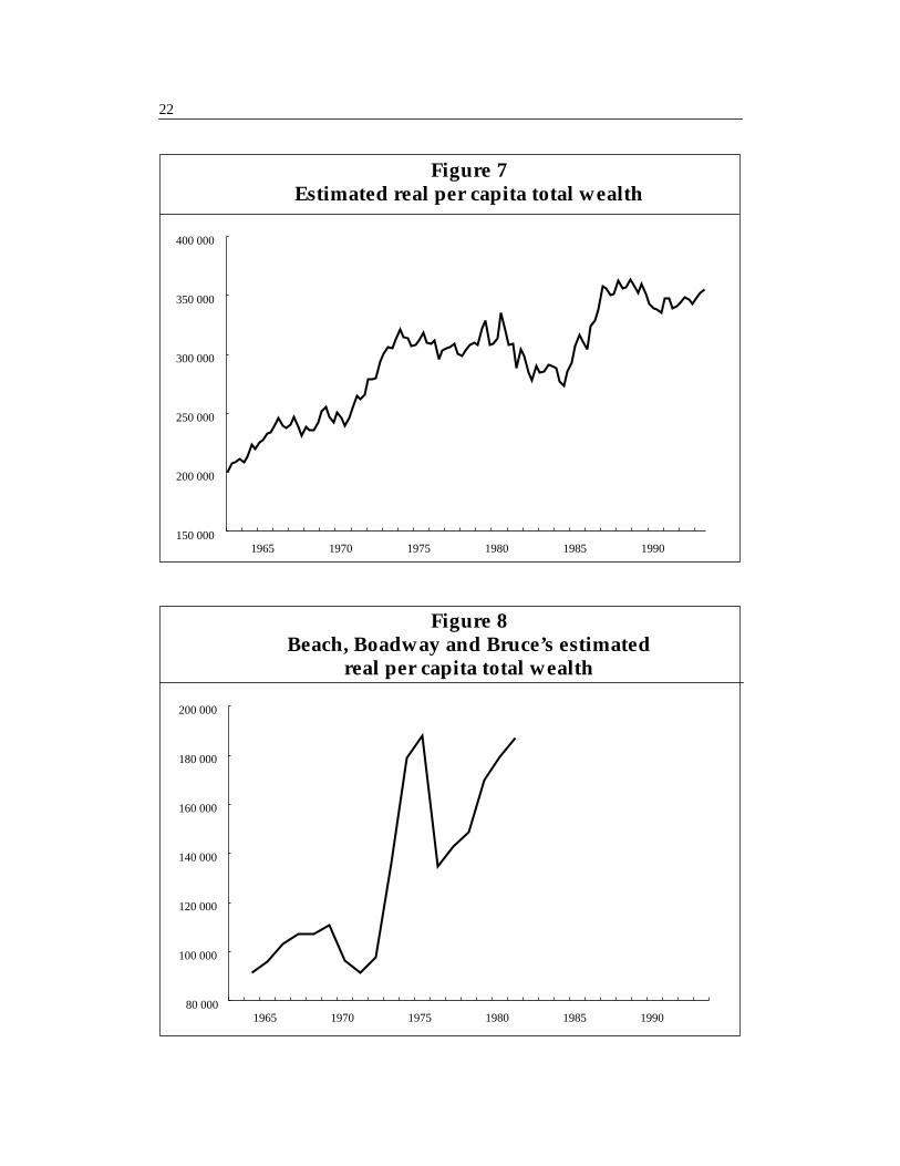
Figure 5 plots the constructed non-human wealth series. Non-human wealth has a more pronounced upward trend than does humanwealth. Relative to Beach, Boadway and Bruce’s measure of non-humanwealth (Figure 6), which is defined as the sum of the sheltered and unshel-tered capital stock series, the new measure shows more growth throughthe late 1960s, but the broad trends are similar. The new series reveal thatfluctuations in non-human wealth have been considerably more pro-nounced since the end of the 1970s. The three main downturns in the newnon-human wealth series coincide with the 1981–82 recession, the October1987 stock market crash and the 1990–91 recession. Note also that each ofthese drops in non-human wealth follows a period of significantly above-average growth in non-human wealth. In terms of its relative size, non-human wealth is on average about one-sixth the size of human wealth.Thus, total wealth, which is depicted in Figure 7, looks more similar tohuman wealth than to non-human wealth. Figure 8 depicts Beach, Boad-way and Bruce’s total wealth series by way of comparison.

21

1965 1970 1975 1980 1985 19906 000

8 000

10 000

12 000

14 000

16 000

18 000

Figure 5Estimated real per capita non-human wealth

Figure 6Beach, Boadway and Bruce’s estimated

real per capita non-human wealth

1965 1970 1975 1980 1985 199010 000

20 000

30 000

40 000

50 000

60 000

70 000

80 000

excluding equity

22

1965 1970 1975 1980 1985 1990150 000

200 000

250 000

300 000

350 000

400 000

1965 1970 1975 1980 1985 199080 000

100 000

120 000

140 000

160 000

180 000

200 000

Figure 7Estimated real per capita total wealth

Figure 8Beach, Boadway and Bruce’s estimated

real per capita total wealth

23

3 IS WEALTH USEFUL IN EXPLAININGCONSUMPTION?

Reliable measures of aggregate human and non-human wealth are poten-tially useful for addressing a broad range of macro issues, but perhapstheir most obvious application is in determining consumption and savings.Specifically, one might ask, is measured wealth useful in explaining thetime-series behaviour of aggregate consumption?

An alternative model with a long tradition in macroeconomics is theKeynesian consumption function that specifies consumption as a functionof disposable income. The usefulness of wealth in explaining consumptionis therefore evaluated relative to this alternative over both long and shorthorizons. The long-run analysis examines the relationship between con-sumption, wealth and disposable income using static linear regressionsand standard tests for cointegration. This long-run analysis then serves as aprecursor for the estimation of EC consumption equations designed toexplain the short-run dynamics of consumption around its long-run trend.

At the outset it is worth stressing that this approach to assessing theusefulness of wealth is relatively stringent, since the disposable-incomeand wealth-based consumption functions may be (nearly) observationallyequivalent. If innovations in disposable income are permanent or at leastvery persistent, then most of the information regarding their future path,and thus the information embodied in human wealth, is contained in thecurrent observations of disposable income. Indeed, using Monte Carlo sim-ulations, Davidson and Hendry (1981) have shown that Hall’s (1978) ran-dom-walk model and the EC models developed by Davidson et al. (1978)and Hendry and von Ungern-Sternberg (1981) are nearly equivalent.

Moreover, at a theoretical level, both Campbell (1987) andMitchener (1984) have demonstrated that a cointegrating relationshipbetween consumption and disposable income is consistent with the lifecycle–permanent income model. The results below cannot, therefore, beviewed as definitive tests of the permanent income model. Rather, theyaddress the more modest question: Does measured wealth provide

24

significant explanatory power for consumption beyond the informationalready contained in disposable income?

3.1 Long-run analysis

Unit root and cointegration tests are used to examine the long-run relation-ship between consumption, wealth and disposable income. Three basiccointegrating relationships are considered: a long-run Keynesian con-sumption function, a wealth-based consumption function, and a hybridmodel that includes both disposable income and wealth. All three alterna-tives are specified in log-linear form:

(3.1)

(3.2)

(3.3)

where c is the log of real per capita consumption on non-durables and serv-ices, y is real per capita disposable income, p is the price of consumption ofnon-durables and services relative to the price of GDP, and w is the log ofreal per capita total wealth. Disposable income, like wealth, is measured inreal terms by deflating by means of the GDP deflator. In order to permithuman and non-human wealth to have different effects on consumptionand to minimize the impact of any level errors in the measurement ofeither component of wealth, versions of (3.2) and (3.3) are also considered,with human wealth (h) and non-human wealth (k) entered separately.

All the variables are measured at a quarterly frequency and are sea-sonally adjusted (see Appendix 1 for details). Table 4 reports the results ofunit root tests. For c, y, w, h, and p the ADF and PP tests provide no evi-dence against the null of a unit root, but reject the null of a unit root in thefirst-differences of these variables. This suggests that these variables are allintegrated of order one, that is, they are I(1), and it is appropriate toexamine the possibility that they are cointegrated. Non-human wealth, in

ct α0 α1yt α2pt υt+ + +=

ct γ0 γ1wt γ2pt νt+ + +=

ct δ0 δ1yt δ2wt δ3pt ϑt+ + + +=

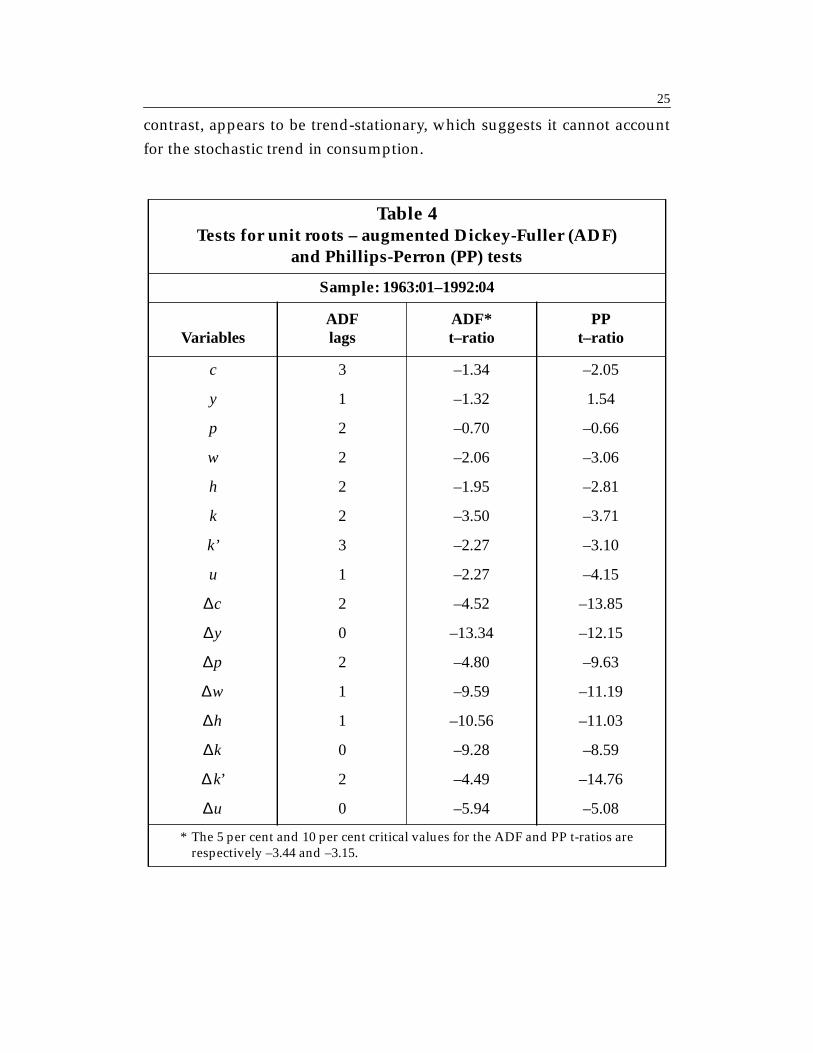
25

contrast, appears to be trend-stationary, which suggests it cannot accountfor the stochastic trend in consumption.

Table 4Tests for unit roots – augmented Dickey-Fuller (ADF)

and Phillips-Perron (PP) tests

Sample: 1963:01–1992:04

VariablesADFlags

ADF*t–ratio

PPt–ratio

c 3 –1.34 –2.05

y 1 –1.32 1.54

p 2 –0.70 –0.66

w 2 –2.06 –3.06

h 2 –1.95 –2.81

k 2 –3.50 –3.71

k’ 3 –2.27 –3.10

u 1 –2.27 –4.15

2 –4.52 –13.85

0 –13.34 –12.15

2 –4.80 –9.63

1 –9.59 –11.19

1 –10.56 –11.03

0 –9.28 –8.59

k’ 2 –4.49 –14.76

0 –5.94 –5.08

* The 5 per cent and 10 per cent critical values for the ADF and PP t-ratios arerespectively –3.44 and –3.15.

∆c

∆y

∆p

∆w

∆h

∆k

∆

∆u

26

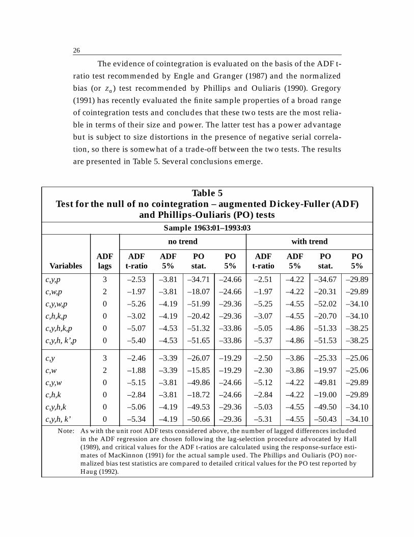
The evidence of cointegration is evaluated on the basis of the ADF t-ratio test recommended by Engle and Granger (1987) and the normalizedbias (or ) test recommended by Phillips and Ouliaris (1990). Gregory(1991) has recently evaluated the finite sample properties of a broad rangeof cointegration tests and concludes that these two tests are the most relia-ble in terms of their size and power. The latter test has a power advantagebut is subject to size distortions in the presence of negative serial correla-tion, so there is somewhat of a trade-off between the two tests. The resultsare presented in Table 5. Several conclusions emerge.

Table 5Test for the null of no cointegration – augmented Dickey-Fuller (ADF)

and Phillips-Ouliaris (PO) testsSample 1963:01–1993:03

no trend with trend

VariablesADFlags

ADFt-ratio

ADF5%

POstat.

PO5%

ADFt-ratio

ADF5%

POstat.

PO5%

c,y,p 3 –2.53 –3.81 –34.71 –24.66 –2.51 –4.22 –34.67 –29.89

c,w,p 2 –1.97 –3.81 –18.07 –24.66 –1.97 –4.22 –20.31 –29.89

c,y,w,p 0 –5.26 –4.19 –51.99 –29.36 –5.25 –4.55 –52.02 –34.10

c,h,k,p 0 –3.02 –4.19 –20.42 –29.36 –3.07 –4.55 –20.70 –34.10

c,y,h,k,p 0 –5.07 –4.53 –51.32 –33.86 –5.05 –4.86 –51.33 –38.25

c,y,h, k’,p 0 –5.40 –4.53 –51.65 –33.86 –5.37 –4.86 –51.53 –38.25

c,y 3 –2.46 –3.39 –26.07 –19.29 –2.50 –3.86 –25.33 –25.06

c,w 2 –1.88 –3.39 –15.85 –19.29 –2.30 –3.86 –19.97 –25.06

c,y,w 0 –5.15 –3.81 –49.86 –24.66 –5.12 –4.22 –49.81 –29.89

c,h,k 0 –2.84 –3.81 –18.72 –24.66 –2.84 –4.22 –19.00 –29.89

c,y,h,k 0 –5.06 –4.19 –49.53 –29.36 –5.03 –4.55 –49.50 –34.10

c,y,h, k’ 0 –5.34 –4.19 –50.66 –29.36 –5.31 –4.55 –50.43 –34.10Note: As with the unit root ADF tests considered above, the number of lagged differences included

in the ADF regression are chosen following the lag-selection procedure advocated by Hall(1989), and critical values for the ADF t-ratios are calculated using the response-surface esti-mates of MacKinnon (1991) for the actual sample used. The Phillips and Ouliaris (PO) nor-malized bias test statistics are compared to detailed critical values for the PO test reported byHaug (1992).

Zα

27

First, there is little evidence that consumption is cointegrated witheither total wealth or its human and non-human components – both theADF test and the Phillips-Ouliaris (PO) test fail to reject the null of nocointegration at even a 10 per cent level.

Second, the evidence that consumption is cointegrated with dispos-able income is mixed. The ADF tests fails to reject the null of no cointegra-tion at a 10 per cent level, while the PO test rejects the same null at the 5 percent level.

Third, when disposable income and either total wealth or humanand non-human wealth are included in the cointegrating vector, there ismore convincing evidence of cointegration. Both the ADF and PO statisticsreject the null of no cointegration at the 5 per cent level in all the long-runregressions that include wealth, and for the PO statistic this null is alsorejected at the 1 per cent level. The one caveat is that the ADF statistics aresomewhat sensitive to the number of lagged differences that are includedin the ADF regression, but this problem should be minimized through useof the lag-length selection procedure advocated by Hall (1989).

A fourth finding is that the relative price of consumption p plays aminor role in the cointegration results. The lower panel of Table 5 reportsthe results when p is omitted from the cointegrating vector, and the test sta-tistics change very little. Overall, the results suggest that both disposableincome and wealth are important long-run determinants of consumption,while the relative price of consumption is not. An examination of thecointegrating vector itself bolsters this conclusion.

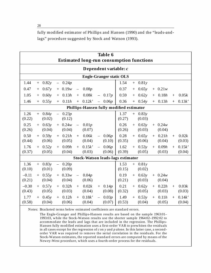
Table 6 reports the estimated long-run coefficients on disposableincome, wealth and the relative price of consumption. The top panel of thetable reports the Engle-Granger static ordinary least squares (OLS) esti-mates on which the Table 5 cointegration tests are based. These parameterestimates, while super-consistent (Engle and Granger 1987), are not effi-cient, and their distributions are unknown. To obtain more efficient esti-mates and perform valid inference on the long-run parameters, thecointegrating parameters are also estimated by means of the prewhitened

28

fully modified estimator of Phillips and Hansen (1990) and the “leads-and-lags” procedure suggested by Stock and Watson (1993).

Table 6Estimated long-run consumption functions

Dependent variable: c

Engle-Granger static OLS

1.44 + 0.82y – 0.24p 1.54 + 0.81y

0.47 + 0.67y + 0.19w – 0.08p 0.37 + 0.65y + 0.21w

1.05 + 0.60y + 0.13h + 0.08k – 0.17p 0.59 + 0.62y + 0.18h + 0.05k

1.46 + 0.55y + 0.11h + 0.12k’ – 0.06p 0.36 + 0.54y + 0.13h + 0.13k’

Phillips-Hansen fully modified estimator

1.26(0.22)

+ 0.84y(0.02)

– 0.23p(0.12)

1.37(0.27)

+ 0.83y(0.03)

0.25(0.26)

+ 0.63y(0.04)

+ 0.24w(0.04)

– 0.01p(0.07)

0.26(0.26)

+ 0.63y(0.03)

+ 0.24w(0.04)

0.50(0.44)

+ 0.59y(0.06)

+ 0.21h(0.05)

+ 0.06k(0.04)

– 0.06p(0.10)

0.28(0.35)

+ 0.65y(0.06)

+ 0.21h(0.04)

+ 0.02k(0.03)

1.76(0.37)

+ 0.52y(0.05)

+ 0.09h(0.04)

+ 0.15k’(0.03)

– 0.06p(0.06)

1.62(0.39)

+ 0.53y(0.05)

+ 0.09h(0.03)

+ 0.15k’(0.04)

Stock-Watson leads-lags estimator

1.36(0.10)

+ 0.83y(0.01)

– 0.20p(0.09)

1.53(0.15)

+ 0.81y(0.02)

–0.11(0.21)

+ 0.55y(0.04)

+ 0.33w(0.04)

– 0.04p(0.06)

0.19(0.21)

+ 0.63y(0.03)

+ 0.24w(0.04)

–0.30(0.43)

+ 0.57y(0.05)

+ 0.32h(0.03)

+ 0.02k(0.04)

+ 0.14p(0.08)

0.21(0.32)

+ 0.62y(0.05)

+ 0.22h(0.03)

+ 0.03k(0.03)

1.77(0.58)

+ 0.45y(0.04)

+ 0.12h(0.06)

+ 0.18k’(0.04)

– 0.03p(0.07)

1.49(0.53)

+ 0.53y(0.04)

+ 0.11h(0.05)

+ 0.14k’(0.04)

Notes: Bracketed terms below estimated coefficients are standard errors.The Engle-Granger and Phillips-Hansen results are based on the sample 1963:01–1993:03, while the Stock-Watson results use the shorter sample 1964:02–1992:02 toaccommodate the leads and lags that are included in the regression. The Phillips-Hansen fully modified estimation uses a first-order VAR to prewhiten the residualsin all cases except for the regression of c on y and p alone. In this latter case, a second-order VAR was required to remove the serial correlation in the residuals. For theStock-Watson estimates, the reported standard errors are computed by means of theNewey-West procedure, which uses a fourth-order process for the residuals.

29

Both estimators correct for the endogeneity bias that is likely to bepresent in this application, given that the right-hand-side variables areunlikely to be strictly exogenous, and both have the same asymptotic dis-tributions. In all but one case, the Phillips-Hansen estimator uses residualsthat are prewhitened with a VAR(1) to correct for serial correlation, sincethe first-order VAR is sufficient to capture most of the serial correlation inthe residuals. The exception is the regression of c on y and p, whichrequired a second-order VAR.

The Stock-Watson procedure is implemented using leads and lags offour quarters, and the reported standard errors are based on the Neweyand West (1987) procedure, since there is evidence of serially correlatedresiduals. Four features of the results stand out.

First, the estimates for which valid standard errors are reportedindicate that both disposable income and wealth are significant determi-nants of trend movements in consumption at any reasonable level ofsignificance.7

Second, while including wealth among the right-hand-side varia-bles reduces the coefficient on disposable income considerably, disposableincome remains an important determinant of consumption. In the simpleKeynesian model, the coefficient on disposable income is always slightlyabove 0.80; when wealth is added, this coefficient ranges from 0.45 to 0.65.

Third, almost all the explanatory power of wealth is coming fromthe human wealth component – the coefficient on non-human wealth (k)while positive, is small and within a standard error of zero. This finding isconsistent with the evidence that non-human wealth is I(0), and cannottherefore explain the stochastic trend in consumption. Consumers,cognizant of the fact that fluctuations in non-human wealth are temporary

7. In contrast, Beach, Boadway and Bruce’s measures of total, human and non-humanwealth were not found to be significant determinants of consumption of non-durables andservices when they were added to a Keynesian consumption function estimated on annualdata from 1964 to 1981 – the frequency and sample for which Beach, Boadway and Bruce’swealth measures are available.

30

shocks, view fluctuations in non-human wealth as transitory income andtherefore absorb them through savings.

This latter finding deserves more scrutiny. Disaggregating non-human wealth into its principal components reveals that fluctuations innon-human wealth are dominated by changes in equity prices. Equitycomprises about one-quarter of non-human wealth on average and is byfar its most volatile component. Note, in particular, the sharp drop in non-human wealth following the October 1987 stock market crash (Figure 5).

This importance of equity for the stochastic behaviour of total non-human wealth suggests at least two interpretations of the weak link fromnon-human wealth to consumption. Consumers may view much of thevolatility in equity prices as short-run in nature, and therefore “seethrough” fluctuations in equity prices when making consumptiondecisions.

Alternatively, aggregate consumption may respond very little tochanges in equity prices simply because a majority of people do not holdequity. Mankiw and Zeldes (1990) point out that only about one-fourth ofAmerican households own stocks. Moreover, they find that the consump-tion of stockholders in the United States is in fact more highly correlatedwith stock returns than is the consumption of non-stockholders. AssumingCanadian households are similar to their American counterparts, the lowcorrelation between consumption and non-human wealth may reflect thesedistributional issues.

To test the possibility that the weak link between non-human wealthand consumption stems largely from equity, an alternative measure of non-human wealth (k’) that does not include equity is constructed. In contrastto total non-human wealth, this alternative variable appears to be I(1), bothon the basis of a simple inspection of the series (see Figure 5) and more for-mal tests. As reported in Table 4, ADF and PP tests on k’ fail to reject thenull of a unit root at the 10 per cent level, although the PP statistic is close.Cointegration tests reported in Table 5 suggest that consumption iscointegrated with y, h and k’, but the more interesting results are the

31

cointegrating parameters reported in Table 6. Note that when k’ is substi-tuted for k, non-human wealth has significant explanatory power for con-sumption based on the Phillips-Hansen and Stock-Watson estimates, andall three estimation techniques produce very similar coefficient estimates.Moreover, when the value of equity is entered separately with the con-sumption function including y, h and k’, it has a negative coefficient that isstatistically indistinguishable from zero. The suggestion is that once werestrict attention to assets such as housing, currency and deposits, whichhave less variable returns and are more widely held, fluctuations in bothhuman and non-human wealth have important effects on consumption.

A fourth noteworthy result in Table 6 is that while the coefficient onthe relative price of consumption is typically negatively signed asexpected, it is only significant in the Keynesian consumption function.Moreover, even in the Keynesian consumption function, the coefficient onthe relative price variable is significantly below that on disposable income(which is nominal disposable income deflated by the GDP deflator). Thissuggests that the GDP deflator is preferred empirically in both theKeynesian and wealth-based consumption functions.

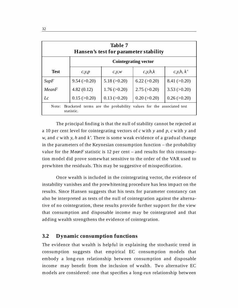
The above inferences all assume that the long-run parametersreported in Table 6 are constant, but if in fact they are changing throughtime, these inferences are invalid. In order to test for this type ofmisspecification, Hansen’s (1992) tests for parameter non-constancy for I(1)processes are applied to the three most interesting long-run equations.Hansen proposes three tests – SupF, MeanF and Lc – which all share the nullof parameter constancy but differ in their alternatives. SupF tests for astructural break of unknown timing and is therefore appropriate for deter-mining if there has been a swift shift in regime, while MeanF and Lc modelthe parameters as a martingale under the alternative, so change is viewedas a gradual process. The test statistics together with their probability val-ues are reported in Table 7 and refer to the Phillips-Hansen parameter esti-mates reported in Table 6.

32

The principal finding is that the null of stability cannot be rejected ata 10 per cent level for cointegrating vectors of c with y and p, c with y andw, and c with y, h and k’. There is some weak evidence of a gradual changein the parameters of the Keynesian consumption function – the probabilityvalue for the MeanF statistic is 12 per cent – and results for this consump-tion model did prove somewhat sensitive to the order of the VAR used toprewhiten the residuals. This may be suggestive of misspecification.

Once wealth is included in the cointegrating vector, the evidence ofinstability vanishes and the prewhitening procedure has less impact on theresults. Since Hansen suggests that his tests for parameter constancy canalso be interpreted as tests of the null of cointegration against the alterna-tive of no cointegration, these results provide further support for the viewthat consumption and disposable income may be cointegrated and thatadding wealth strengthens the evidence of cointegration.

3.2 Dynamic consumption functions

The evidence that wealth is helpful in explaining the stochastic trend inconsumption suggests that empirical EC consumption models thatembody a long-run relationship between consumption and disposableincome may benefit from the inclusion of wealth. Two alternative ECmodels are considered: one that specifies a long-run relationship between

Table 7Hansen’s test for parameter stability

Cointegrating vector

Test c,y,p c,y,w c,y,h,k c,y,h, k’

SupF 9.54 (>0.20) 5.18 (>0.20) 6.22 (>0.20) 8.41 (>0.20)

MeanF 4.82 (0.12) 1.76 (>0.20) 2.75 (>0.20) 3.53 (>0.20)

Lc 0.15 (>0.20) 0.13 (>0.20) 0.20 (>0.20) 0.26 (>0.20)

Note: Bracketed terms are the probability values for the associated teststatistic.

33

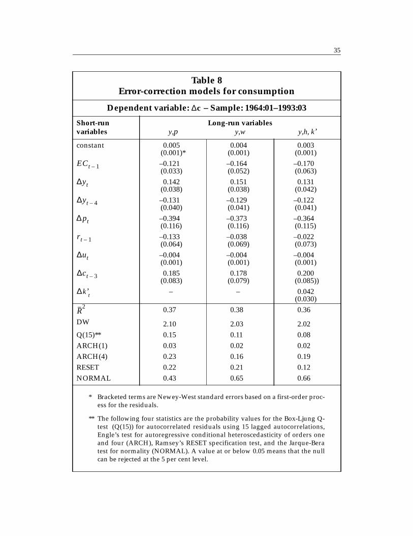
consumption, disposable income and total wealth, and a second that entershuman wealth and non-human wealth (excluding equity) separately. As abasis of comparison, a traditional EC model that excludes wealth is alsoestimated.

The dependent variable in all the dynamic equations is the first dif-ference of consumption, and it depends on the first lag of the OLS esti-mates of the residual in the long-run consumption function – the EC term –and the current and lagged first differences of the long-run determinants ofconsumption. The coefficient on the EC term should be significantly lessthan zero if c is cointegrated with its long-run explanatory variables. Addi-tional variables can also be included in the dynamic equation if these vari-ables are thought to exert a short-run influence on consumption.

Empirical studies over the past decade and a half have furnished anexpansive and colourful menu of would-be regressors that are likely tocontribute to short-run fluctuations in consumption around its long-runtrend. The present analysis, however, confines the specification search totwo of the most popular explanatory variables: the real interest rate andthe unemployment rate or its first difference.

The interest rate is typically included to capture both the wealtheffect associated with revaluations of human and non-human wealth (sincewealth is not usually included in the regression) and the intertemporalsubstitution effect associated with fluctuations in the relative price of cur-rent versus future consumption. In principle, the sign of the interest rateeffect is ambiguous, but the usual presumption is that it is negative. Theextended EC models considered here that include wealth provide theopportunity to separate the revaluation effect from the intertemporal sub-stitution effect. The unemployment rate is generally thought to proxyeither liquidity effects or uncertainty and its expected sign is thereforenegative.

In order to ensure that the impact of these short-run variables is infact confined to the short run, they should be I(0). The real interest rate andthe unemployment rate are therefore pretested for stationarity. Evidence

34

supporting the stationarity of the real interest rate was discussed above inthe measurement of wealth and is presented in Table 1. The results fromADF and PP unit root tests on the unemployment rate and its firstdifference are reported in Table 4. The null of a unit root in the first differ-ence of the unemployment rate is convincingly rejected, but the ADF andPP tests give conflicting results in the case of the level of the unemploy-ment rate, so both u and are considered.

The estimation of the dynamic consumption function began withfourth-order lags on all right-hand-side dynamic variables and was thensequentially simplified with the aim of producing a parsimonious equationwith sensible economic properties, reasonable fit and well-behaved residu-als. The estimated final-form dynamic equations are reported in Table 8.

The impact of including wealth in the EC model is best discussedwith reference to the standard EC model in which the long-run behaviourof consumption is determined by disposable income alone. Results for thismodel are presented in the second column of Table 8; several features arenoteworthy.

The EC term is negatively signed and significant at the 1 per centlevel, which is consistent with evidence of cointegration. The estimatedcoefficients on the first difference of the relative price of consumption, thereal interest rate and the change in the unemployment rate are all nega-tively signed as expected and significant at the 5 per cent level. The statisti-cal significance of the coefficients on the third lag of the dependent variableand the fourth lag of the first difference of disposable income is difficult tointerpret but is consistent with rejections of Hall’s (1978) random walkmodel. Finally, the residual diagnostics reported at the bottom of Table 8suggest that autoregressive conditional heteroscedasticity is a feature ofthe residuals. Accordingly, heteroscedastic-consistent standard errors arereported based on the Newey-West procedure.

∆u

35

Table 8Error-correction models for consumption

Dependent variable: – Sample: 1964:01–1993:03

Short-run Long-run variablesvariables y,p y,w y,h, k’

constant 0.005(0.001)*

0.004(0.001)

0.003(0.001)

–0.121(0.033)

–0.164(0.052)

–0.170(0.063)

0.142(0.038)

0.151(0.038)

0.131(0.042)

–0.131(0.040)

–0.129(0.041)

–0.122(0.041)

–0.394(0.116)

–0.373(0.116)

–0.364(0.115)

–0.133(0.064)

–0.038(0.069)

–0.022(0.073)

–0.004(0.001)

–0.004(0.001)

–0.004(0.001)

0.185(0.083)

0.178(0.079)

0.200(0.085))

k’t – – 0.042(0.030)

0.37 0.38 0.36

DW 2.10 2.03 2.02Q(15)** 0.15 0.11 0.08ARCH(1) 0.03 0.02 0.02ARCH(4) 0.23 0.16 0.19RESET 0.22 0.21 0.12NORMAL 0.43 0.65 0.66

* Bracketed terms are Newey-West standard errors based on a first-order proc-ess for the residuals.

** The following four statistics are the probability values for the Box-Ljung Q-test (Q(15)) for autocorrelated residuals using 15 lagged autocorrelations,Engle’s test for autoregressive conditional heteroscedasticity of orders oneand four (ARCH), Ramsey’s RESET specification test, and the Jarque-Beratest for normality (NORMAL). A value at or below 0.05 means that the nullcan be rejected at the 5 per cent level.

∆c

ECt 1–

∆yt

∆yt 4–

∆ pt

r t 1–

∆ut

∆ct 3–

∆

R2

36

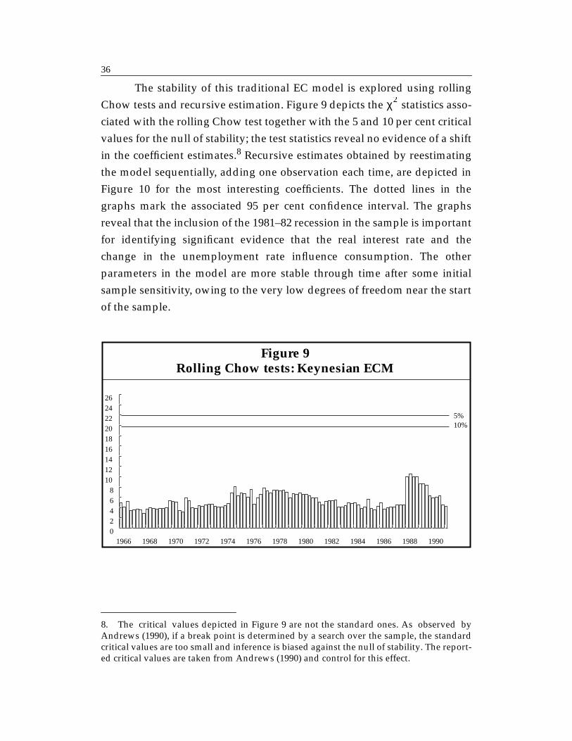
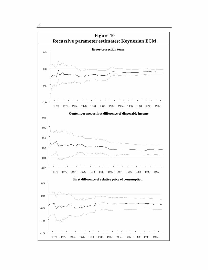
The stability of this traditional EC model is explored using rollingChow tests and recursive estimation. Figure 9 depicts the statistics asso-ciated with the rolling Chow test together with the 5 and 10 per cent criticalvalues for the null of stability; the test statistics reveal no evidence of a shiftin the coefficient estimates.8 Recursive estimates obtained by reestimatingthe model sequentially, adding one observation each time, are depicted inFigure 10 for the most interesting coefficients. The dotted lines in thegraphs mark the associated 95 per cent confidence interval. The graphsreveal that the inclusion of the 1981–82 recession in the sample is importantfor identifying significant evidence that the real interest rate and thechange in the unemployment rate influence consumption. The otherparameters in the model are more stable through time after some initialsample sensitivity, owing to the very low degrees of freedom near the startof the sample.

8. The critical values depicted in Figure 9 are not the standard ones. As observed byAndrews (1990), if a break point is determined by a search over the sample, the standardcritical values are too small and inference is biased against the null of stability. The report-ed critical values are taken from Andrews (1990) and control for this effect.

χ2

Figure 9Rolling Chow tests: Keynesian ECM

1966 1968 1970 1972 1974 1976 1978 1980 1982 1984 1986 1988 199002468

101214161820222426

5%10%

37

38

First difference of relative price of consumption

Error-correction term

1970 1972 1974 1976 1978 1980 1982 1984 1986 1988 1990 1992–1.0

–0.5

0.0

0.5

1970 1972 1974 1976 1978 1980 1982 1984 1986 1988 1990 1992–0.2

0.0

0.2

0.4

0.6

0.8

1970 1972 1974 1976 1978 1980 1982 1984 1986 1988 1990 1992–1.5

–1.0

–0.5

0.0

0.5

Figure 10Recursive parameter estimates: Keynesian ECM

Contemporaneous first difference of disposable income

39

The second-column results in Table 8 present an estimated ECmodel that is based on a long-run consumption function that includes bothdisposable income and total wealth. The most noticeable feature of thisdynamic consumption function is that the EC term is larger in magnitude;this is consistent with the stronger evidence of cointegration reported inTable 5 when wealth is included.

A second feature of the EC model that includes wealth is that thecoefficient on the real interest rate is about a third as large as in the Keyne-sian model, and is now no longer significantly different from zero at

1970 1972 1974 1976 1978 1980 1982 1984 1986 1988 1990 1992–1.5

–1.0

–0.5

0.0

0.5

1.0

1.5

1970 1972 1974 1976 1978 1980 1982 1984 1986 1988 1990 1992–0.020

–0.015

–0.010

–0.005

0.000

0.005

0.010

0.015

Figure 10 (continued)

First difference of real interest rate

First difference of unemployment rate

40

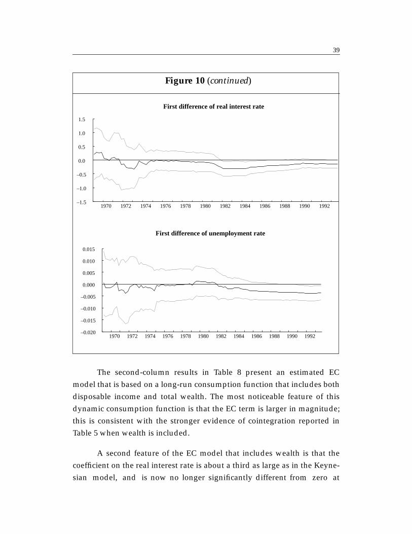
conventional levels. Presumably this reduced interest rate effect reflects thefact that the inclusion of wealth in the equation absorbs the wealth effect ofinterest rate changes, leaving only the pure substitution effect to be pickedup by the coefficient on the real interest rate. The point estimates thereforesuggest that most of the interest rate effect in the Keynesian equation isdue to the wealth effect.

Third, note that the coefficient on the first difference of the relativeprice of consumption is virtually unaffected by the inclusion of wealth, sowhile relative price effects are captured by wealth in the long run, the rela-tive price of consumption has significant dynamic effects on consumption.Finally, the third column of Table 8 considers the impact of substitutingtotal wealth in the cointegrating vector for human wealth and non-humanwealth (excluding equity) entered separately. The impact of this substitu-tion is relatively minor; the coefficient on the real interest rate falls margin-ally and there is a small dynamic effect of changes in non-human wealth.

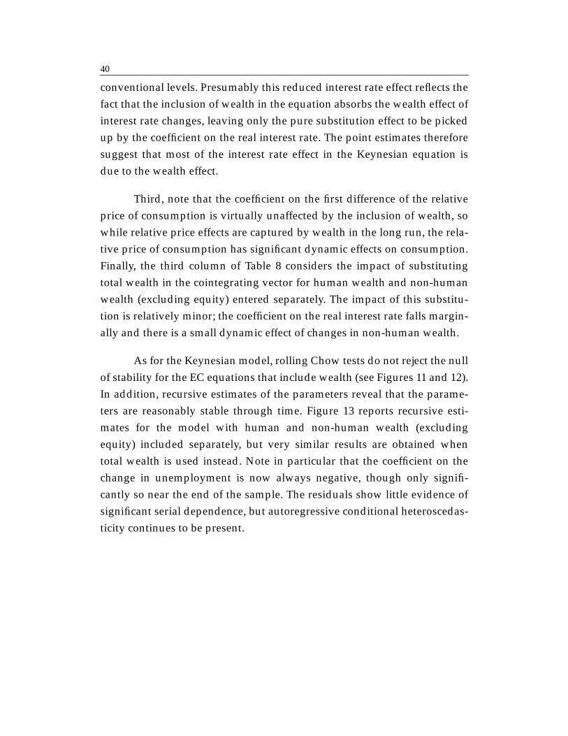
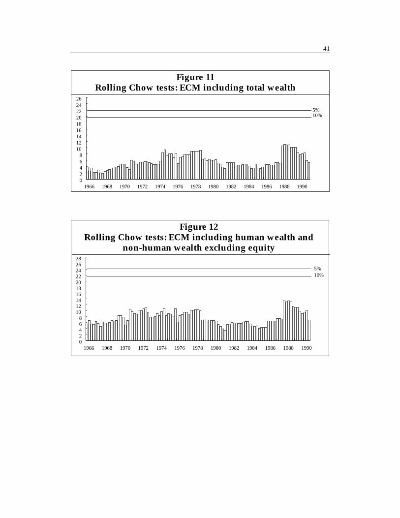
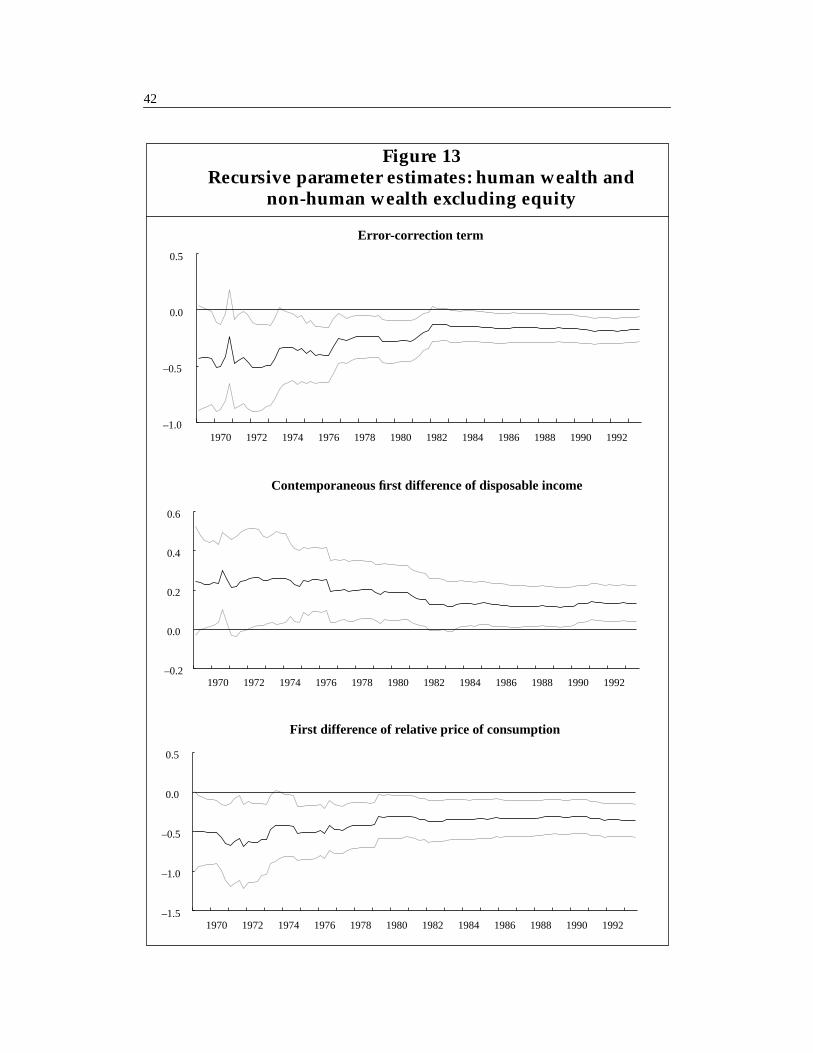
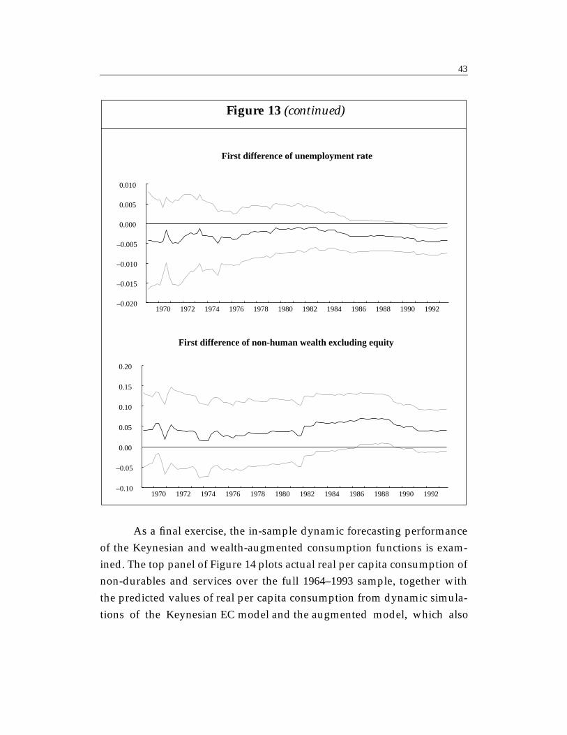
As for the Keynesian model, rolling Chow tests do not reject the nullof stability for the EC equations that include wealth (see Figures 11 and 12).In addition, recursive estimates of the parameters reveal that the parame-ters are reasonably stable through time. Figure 13 reports recursive esti-mates for the model with human and non-human wealth (excludingequity) included separately, but very similar results are obtained whentotal wealth is used instead. Note in particular that the coefficient on thechange in unemployment is now always negative, though only signifi-cantly so near the end of the sample. The residuals show little evidence ofsignificant serial dependence, but autoregressive conditional heteroscedas-ticity continues to be present.

41

Figure 11Rolling Chow tests: ECM including total wealth

1966 1968 1970 1972 1974 1976 1978 1980 1982 1984 1986 1988 199002468

101214161820222426

5%10%

1966 1968 1970 1972 1974 1976 1978 1980 1982 1984 1986 1988 199002468

10121416182022242628

Figure 12Rolling Chow tests: ECM including human wealth and

non-human wealth excluding equity

5%10%

42

1970 1972 1974 1976 1978 1980 1982 1984 1986 1988 1990 1992–0.2

0.0

0.2

0.4

0.6

1970 1972 1974 1976 1978 1980 1982 1984 1986 1988 1990 1992–1.5

–1.0

–0.5

0.0

0.5

Figure 13Recursive parameter estimates: human wealth and

non-human wealth excluding equity

Contemporaneous first difference of disposable income

First difference of relative price of consumption

1970 1972 1974 1976 1978 1980 1982 1984 1986 1988 1990 1992–1.0

–0.5

0.0

0.5

Error-correction term

43

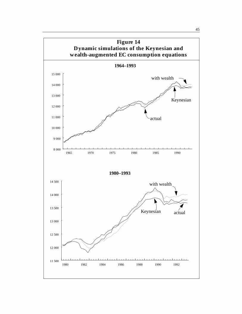
As a final exercise, the in-sample dynamic forecasting performanceof the Keynesian and wealth-augmented consumption functions is exam-ined. The top panel of Figure 14 plots actual real per capita consumption ofnon-durables and services over the full 1964–1993 sample, together withthe predicted values of real per capita consumption from dynamic simula-tions of the Keynesian EC model and the augmented model, which also

1970 1972 1974 1976 1978 1980 1982 1984 1986 1988 1990 1992–0.020

–0.015

–0.010

–0.005

0.000

0.005

0.010

1970 1972 1974 1976 1978 1980 1982 1984 1986 1988 1990 1992–0.10

–0.05

0.00

0.05

0.10

0.15

0.20

First difference of unemployment rate

First difference of non-human wealth excluding equity

Figure 13 (continued)

44

45

1965 1970 1975 1980 1985 19908 000

9 000

10 000

11 000

12 000

13 000

14 000

15 000

1980 1982 1984 1986 1988 1990 199211 500

12 000

12 500

13 000

13 500

14 000

14 500

Figure 14Dynamic simulations of the Keynesian and

wealth-augmented EC consumption equations

1964–1993

1980–1993

actual

Keynesian

with wealth

actualKeynesian

with wealth

46

includes human wealth and non-human wealth (excluding equity).9 Thelower panel of Figure 14 focusses attention on the two most recent businesscycles, reporting dynamic simulations starting in 1980.

The graphs reveal that both EC models track the broad movementsin consumption reasonably well. Prior to the 1980s, the Keynesian ECequation and wealth-augmented model have very similar dynamic fore-casts, but in the 1980s there are some more marked differences. Althoughboth equations underpredict the decline in consumption experienced dur-ing the 1981–82 recession, the equation including wealth explains a consid-erably larger proportion of the observed peak-to-trough decline – 85 percent as compared with only 51 per cent for the Keynesian equation. Theequation including wealth also tracks observed consumption more closelyin the latter half of the 1980s.

Strong growth in both human wealth and non-human wealthexcluding equity through the 1987–88 period results in a considerablyhigher predicted level of consumption by the start of 1989, when wealth isincluded. As a result, the wealth-augmented model does a much better jobof explaining the consumption boom in the late 1980s. This is consistentwith the view that rising asset values, particularly housing prices, fuelledhigh levels of consumption over this period.

Looking at the most recent recession, we see that neither equationcan account for the magnitude of the fall in consumption through 1990 –both equations predict about half the observed decline. For the period fol-lowing the recession, both equations predict little consumption growththrough 1991 and 1992, with a slight pickup in 1993. While actual con-sumption growth remained weak in 1993, the tempting conclusion is thatstronger consumption growth is just around the corner.

9. The dynamic simulations (not shown) for the model using total wealth are very similarthough marginally inferior to those with human and non-human wealth (excluding equity)entered separately.

47

4 CONCLUSION

The wealth measure developed in this study has significant explanatorypower for consumption over and above the information already containedin current disposable income. This suggests that expected future income isan important determinant of consumption for at least some households. Atthe same time, disposable income remains an important determinant ofconsumption in both the short and the long run. One interpretation of thisfinding is that a significant proportion of households are liquidity con-strained and therefore consume out of disposable income. An alternativeinterpretation is that wealth is measured with error, and this error is corre-lated with disposable income. Unfortunately, the results presented in thisstudy cannot be used to discriminate between these two alternatives.

A second finding is that fluctuations in equity prices have no signif-icant impact on aggregate consumption of non-durables and services. Ameasure of non-human wealth that includes equity is found to have littleexplanatory power for consumption in either the long or the short run,while a measure that excludes equity is a significant long-run determinantof consumption. This finding may reflect the fact that most consumers sim-ply do not hold equity or that a large proportion of the changes in equityprices are viewed as transitory.

Estimates of dynamic EC consumption functions suggest that thenegative effect of interest rates on consumption in a traditional Keynesianconsumption function is due principally to the effect of interest rates onhuman wealth. When wealth is included among the regressors, the coeffi-cient on the real interest rate remains negative, owing presumably to anintertemporal substitution effect, but this effect is not significant.

For policy makers and practitioners, the most convincing evidencethat wealth is an important determinant of consumption is probably that itis helpful in explaining both the severity of the 1981–82 recession andconsumption boom of the late 1980s, both of which appear anomalousbased on a traditional EC consumption equation that does not includewealth. While future work will no doubt improve empirical consumption

48

functions further, by augmenting a standard EC consumption model withwealth, this analysis succeeds both in placing empirical consumption mod-els for Canada on a firmer theoretical foundation and in improving ourability to explain observed consumption behaviour.

On a broader level, the usefulness of wealth explaining consump-tion suggests that the measures of wealth developed in this report may beuseful in other applications. These include the impact of public policy onconsumption and saving, and the effect of fluctuations in asset prices onaggregate demand and inflation.

The evidence that aggregate consumption and saving respond dif-ferently to different components of non-human wealth also suggests thatdistributional issues deserve more attention. In principle, heterogeneity inconsumer portfolios could be addressed by disaggregating consumers intovarious groups, but this approach is hampered by the lack of adequatedata. An alternative is to disaggregate non-human wealth into its principalcomponents and examine the sensitivity of these individual components toaggregate consumption.

Evidence that consumption is influenced by the composition ofwealth may also indicate that adjustment costs associated with portfolioallocation differ across assets. In the absence of separation between theportfolio-choice and consumption-savings problems, an integratedapproach to modelling wealth allocation and consumption behaviour isappropriate. These and other extensions, however, are left for future work.

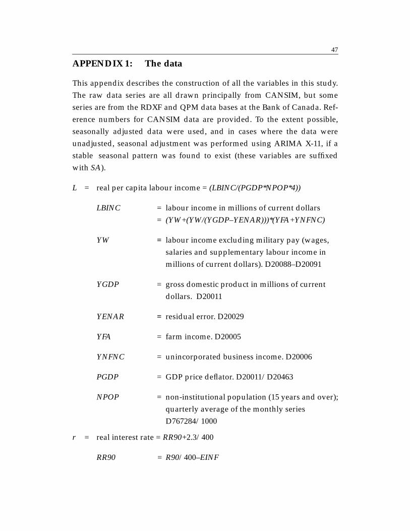
47

APPENDIX 1: The data

This appendix describes the construction of all the variables in this study.The raw data series are all drawn principally from CANSIM, but someseries are from the RDXF and QPM data bases at the Bank of Canada. Ref-erence numbers for CANSIM data are provided. To the extent possible,seasonally adjusted data were used, and in cases where the data wereunadjusted, seasonal adjustment was performed using ARIMA X-11, if astable seasonal pattern was found to exist (these variables are suffixedwith SA).

L = real per capita labour income = (LBINC/(PGDP*NPOP*4))

LBINC = labour income in millions of current dollars= (YW+(YW/(YGDP–YENAR)))*(YFA+YNFNC)

YW = labour income excluding military pay (wages,salaries and supplementary labour income inmillions of current dollars). D20088–D20091

YGDP = gross domestic product in millions of currentdollars. D20011

YENAR = residual error. D20029

YFA = farm income. D20005

YNFNC = unincorporated business income. D20006

PGDP = GDP price deflator. D20011/D20463

NPOP = non-institutional population (15 years and over);quarterly average of the monthly seriesD767284/1000

r = real interest rate = RR90+2.3/400

RR90 = R90/400–EINF

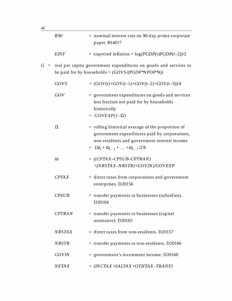
48

R90 = nominal interest rate on 90-day prime corporatepaper. B14017

EINF = expected inflation = log(PGDP(t)PGDP(t–2))/2

G = real per capita government expenditures on goods and services tobe paid for by households = (GOVS/(PGDP*NPOP*4))

GOVS = (GOV(t)+GOV(t–1)+GOV(t–2)+GOV(t–3))/4

GOV = government expenditures on goods and servicesless fraction not paid for by householdshistorically

=

= rolling historical average of the proportion ofgovernment expenditures paid by corporations,non-residents and government interest income

=

= ((CPTAX–CPSUB–CPTRAN)

+(NRSTAX–NRSTR)+GOVIN)/GOVEXP

CPTAX = direct taxes from corporations and governmententerprises. D20156

CPSUB = transfer payments to businesses (subsidies).D20164

CPTRAN = transfer payments to businesses (capitalassistance). D20165

NRSTAX = direct taxes from non-residents. D20157

NRSTR = transfer payments to non-residents. D20166

GOVIN = government’s investment income. D20160

NETAX = (INCTAX+SALTAX+OTHTAX–TRANF)

GOVEXP(1–Ω)

Ω

ωt ωt 1– … +ωt 7–+ +( ) 8⁄

ω

49

TAX = taxes net of transfers= (NETAX/(PGDP*NPOP*4))

INCTAX = direct taxes from persons. D20155

SALTAX = indirect taxes. D20158

OTHTAX = other current transfers from persons. D20159

TRANF = transfer payments to persons. D20163

GOVEXP = current expenditure on goods and services.D20162

A = net domestic foreign assets excluding government debt

= (NETWORTHSA/PGDP*NPOP)

NETWORTHSA = net worth at market value= HOUSESA+FINAQ1SA+EQUITQSA

+HDEBTQSA–HLIABQSA+CQPPQSA

–DDEBTQSA

HOUSESA = non-financial assets of persons andunincorporated businesses. Includes totalconsumer durables and residential structures.

= RSTRUCSA+KDUR

RSTRUC = residential structures = (PMLS/100) * KRC

PMLS = multiple homes listing price index. RDXF database = PMLS

KRC = stock of housing in constant 1986 dollars.QPM data base = KRC

RSTRUCSA = residential structures

50

KDUR = total stock of consumer durables (includesmotor vehicles, household durables andmiscellaneous durables)

= (KMV*PCMV)+(KDHSHD*PHSHD)

+ (KDMISC*PCDMIS)

KMV = stock of motor vehicles held by consumersKMV = 16 734.82 [1960:4]set KMV = 0.933*KMV [t–1]+(D20490/4)

PCMV = price of consumer motor vehicles and parts= (D20115/D20490)

KDHSHD = stock of household durables held by consumersKDHSHD = 9 237.448 [1960:4]set KDHSHD = 0.944*KDHSHD [t–1]

+(D20491/4)

PHSHD = price of consumer household durables= (D20116/D20491)

KDMISC = stock of durables excluding motor vehicles andparts, and household durables held byconsumersKDMISC = 3 539.846 [1960:4]set KDMISC = 0.944*KDMISC [t–1]

+(D20492/4)

PCDMIS = price of other consumer durables= (D20117/D20492)

FINAQ1SA = financial assets of persons and unincorporatedbusinesses (seasonally adjusted). Includescurrency and deposits, consumer credit, otherCanadian bonds (short- and long-term), lifeinsurance and pensions, foreign investments,mortgages and other financial assets.

51

= FINAQ_CD+FINAQ_CC+FINAQ_OBDS

+ FINAQ_LP + FINAQ_FI+FINAQ_OF

+ FINAQ_M

FINAQ_CD = currency and deposits.D160006+D160007+D160008,D150032+D150033+D150034

FINAQ_CC = consumer credit. D160010, D150048

FINAQ_OBDS = other bonds (short- and long-term).D160016+D160022, D150036+D150065

FINAQ_LP = life insurance and pensions. D160023,D150066

FINAQ_FI = foreign investments. D160028, D150068

FINAQ_OF = other financial assets. D160029, D150049

FINAQ_M = mortgages. D160017, D150128

EQUITYQ = market value of equity held by persons andunincorporated businesses

= EQUITYQ(t–1)*TSE_Q(t)/TSE_Q(t–1)

+ (BEQUITY(t)–BEQUITY(t–1))

TSE = TSE300 composite stock price index. B4237

BEQUITY = book value of equity held by persons andunincorporated businesses

= EQUITQ–(YCR/4)*(EQUITQ/TEQUITQ)

EQUITQ = “current” value of shares held by persons andunincorporated businesses. Current value ismeasured as the sum of book value andcumulated retained earnings. D160027, D150067

52

TEQUITQ = total outstanding stock of equity. D162906,D151988

YCR = retained earnings. D20068

HDEBT = book value of government debt held by personsand unincorporated businesses

= HTBQ+HGBQ+HPBQ+HMBQ

HDEBTQ = market value of government debt held bypersons and unincorporated businesses

= HTBQ+PBQ*(HDEBT–HTBQ)

H_BQ = holdings of treasury bills (T), Government ofCanada bonds (G), provincial bonds (P) andmunicipal bonds (M) by persons andunincorporated businesses.D160015, D150035; D160019, D150062;D160020, D150063; D160021, D150064

HLIABQ = total liabilities of persons and unincorporatedbusinesses. Includes consumer credit, tradepayables, bank loans, other loans, finance andother short-term paper, other Canadian bonds,and mortgages. D160031, D150050

NNWPFIQ = net worth of public financial institutions lesstheir holdings of government debt

= NWPFIQ–PFIGBQ–PFIPBQ–PFIMBQ

– PFITBQ

PFI_BQ = holdings of treasury bills (T), government ofCanada bonds (G), provincial bonds (P) andmunicipal bonds (M) by public financialinstitutions.D161975, D151326; D161979, D151330;D161980, D151331; D161981, D151332

53

CPPQ = Canada Pension Plan. D162590, D151760

QPPQ = Quebec Pension Plan. D162660, D151784

CQPPQ = aggregated Canada and Quebec pension plans= (CPPQ+QPPQ)

DDEBTQ = domestically held government debt at marketvalue

= TBILL–FORTBQ+PBG*(OTHDEBT

–FORGBQ–FORPBQ–FORMBQ)

TBILL = net teasury bills outstanding at book value= TTBQ–GTBQ–PGTBQ–PFITBQ–GETBQ

–BCTBQ

TTBQ = total outstanding stock of treasury bills.D162894, D151976

_TBQ = holdings of treasury bills by the federalgovernment (G), provincial governments (PG),public financial institutions (PFI), governmententerprises (GE) and the Bank of Canada (BC).D162185, D151482; D162255, D151544; D161975,D151326; D160155, D150147; D160435, D150350

OTHDEBT = net other debt outstanding at book value= TGBQ+TPBQ+TMBQ–GGBQ–GPBQ–GMBQ

–PGBQ–PPBQ–PMBQ–PFIGBQ–PFIPBQ

–PFIMBQ–GEGBQ–GEPBQ–BCGBQ

T_BQ = total outstanding stock of federal governmentbonds (G), provincial government bonds (P) andmunicipal government bonds (M).D162898, D151980; D162899, D151981;D162900, D151982

54

G_BQ = federal government holdings of federal govern-ment bonds (G), provincial government bonds(P) and municipal government bonds (M).D162189, D151486; D162190, D151487; D162191,D151488

P_BQ = provincial government holdings of federalgovernment bonds (G), provincial governmentbonds (P) and municipal government bonds (M).D162259, D151548; D162260, D151549; D162261,D151550

PFI_BQ = holdings by public financial institutions offederal government bonds (G), provincialgovernment bonds (P) and municipalgovernment bonds (M).D161979, D151330; D161980, D151331;D161981, D151332

GE_BQ = holdings by government enterprises of federalgovernment bonds (G), provincial governmentbonds (P) and municipal government bonds (M).D160159, D150151; D160160, D150152; D160161,D150153

BCGBQ = Bank of Canada’s holdings of federalgovernment bonds. D160439, D150353

PBG = bond price index constructed following Roseand Selody (1985)

= RAC/RG_Q+((1–RAC)/RG_Q)

exp[–RG_Q* (1–RATAX)*19.6]

RG = average yield to maturity on 3–5 yearGovernment of Canada bonds. B14010

RG_Q = quarterly average of the monthly series RG

55

RAC = average coupon rate= RAC(t–1) if (DIFDEBT+1/19.6) < 0= RAC(t–1)*((DEBT(t–1)/DEBT(t))–1/19.6)

+RG*(((DEBT(t)–DEBT(t–1))/DEBT(t))+1/19.6)

otherwise

RATAX = average tax rate = INCTAX/LBINC

DIFDEBT = (DEBT(t)–DEBT(t–1))/(DEBT(t–1)

+DEBT(t))/2+1/19.6

FDEBTQ = foreign debt at market value= (FORTBQ+PBG*(FORGBQ

+FORPBQ+FORMBQ))

FOR_BQ = rest of the world – Government of Canadatreasury bills (T), federal government bonds (G),provincial government bonds (P) and municipalgovernment bonds (M).D162745, D151811; D162749, D151814; D162750,D151815; D162751, D151816

c = log of real per capita consumption of non-durables and services= log [(CON–CDUR)/NPOP]

CON = real total consumption. D20488

CDUR = real consumption of durables. D20489

y = log of real per capita disposable income = log [YDP/PGDP/NPOP]

YDP = current dollar disposable income. D20111

56

p = relative price of non-durables and services= log [((CON$ – CDUR$)/(CON – CDUR))/PGDP]

CON$ = total consumption in current dollars. D20113

CDUR$ = consumption of durables in current dollars.D20114

u = unemployment rate. Statistics Canada, Labour Force Division.(LFSA601/LFSA101)*100

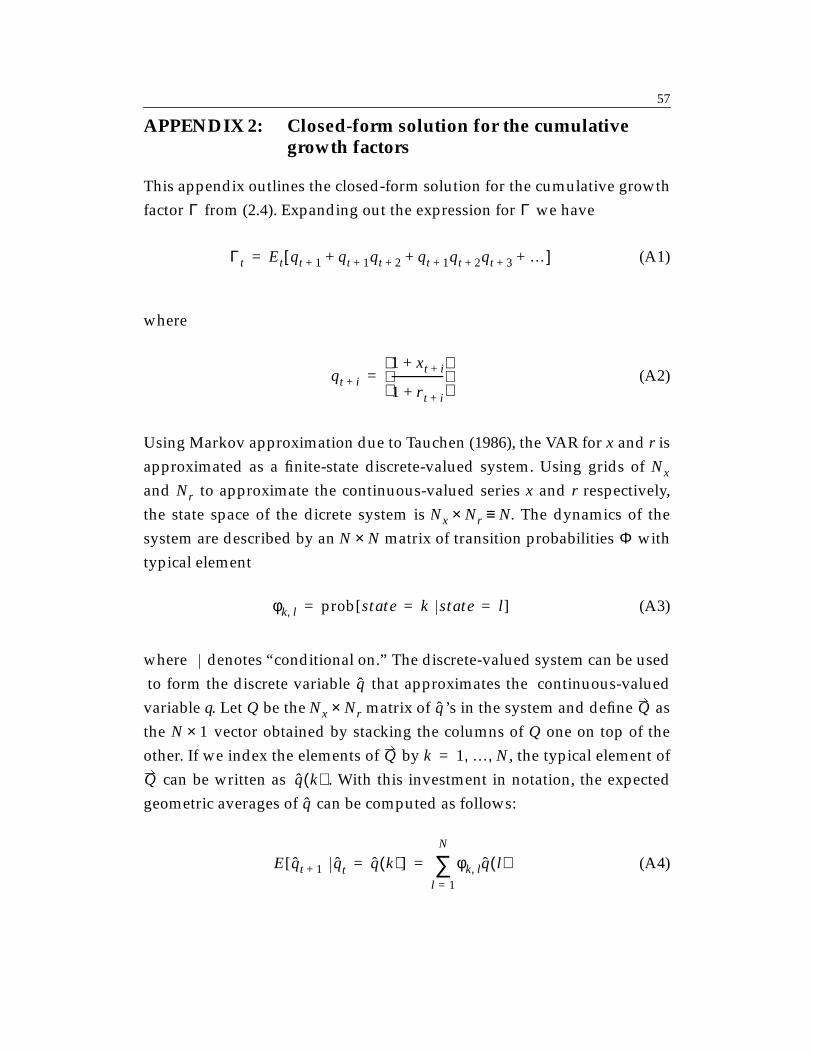
57

APPENDIX 2: Closed-form solution for the cumulativegrowth factors

This appendix outlines the closed-form solution for the cumulative growthfactor from (2.4). Expanding out the expression for we have

(A1)

where

(A2)

Using Markov approximation due to Tauchen (1986), the VAR for x and r isapproximated as a finite-state discrete-valued system. Using grids ofand to approximate the continuous-valued series x and r respectively,the state space of the dicrete system is . The dynamics of thesystem are described by an matrix of transition probabilities withtypical element

(A3)

where denotes “conditional on.” The discrete-valued system can be usedto form the discrete variable that approximates the continuous-valuedvariable q. Let Q be the matrix of ’s in the system and define asthe vector obtained by stacking the columns of Q one on top of theother. If we index the elements of by , the typical element of

can be written as . With this investment in notation, the expectedgeometric averages of can be computed as follows:

(A4)

Γ Γ

Γt Et qt 1+ qt 1+ qt 2+ qt 1+ qt 2+ qt 3+ …+ + +[ ]=

qt i+

1 xt i++

1 r t i++-------------------

=

Nx

Nr

Nx Nr× N≡N N× Φ

φk l, prob[state k state l ]= = =

q

Nx Nr× q Q

N 1×Q k 1 … N, ,=

Q q k( )q

E[ qt 1+ qt q k( )] φk l, q l( )l 1=

N

∑= =

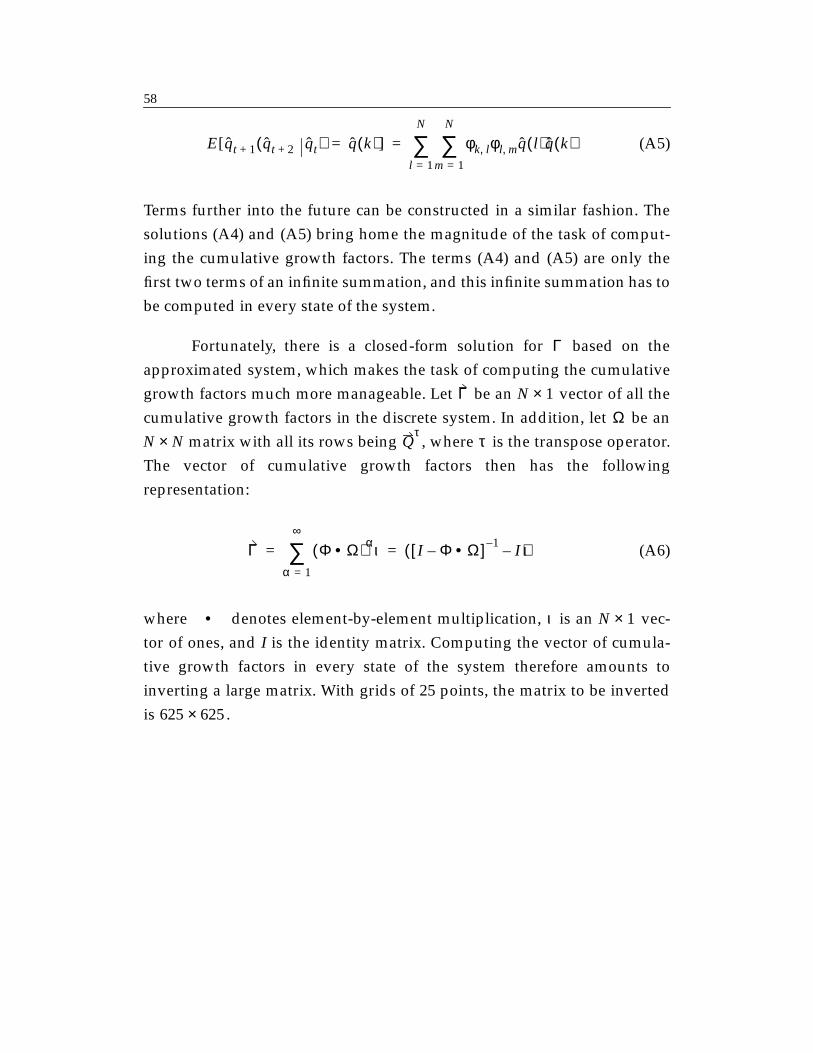
58

(A5)

Terms further into the future can be constructed in a similar fashion. Thesolutions (A4) and (A5) bring home the magnitude of the task of comput-ing the cumulative growth factors. The terms (A4) and (A5) are only thefirst two terms of an infinite summation, and this infinite summation has tobe computed in every state of the system.

Fortunately, there is a closed-form solution for based on theapproximated system, which makes the task of computing the cumulativegrowth factors much more manageable. Let be an vector of all thecumulative growth factors in the discrete system. In addition, let be an

matrix with all its rows being , where is the transpose operator.The vector of cumulative growth factors then has the followingrepresentation:

(A6)

where denotes element-by-element multiplication, is an vec-tor of ones, and I is the identity matrix. Computing the vector of cumula-tive growth factors in every state of the system therefore amounts toinverting a large matrix. With grids of 25 points, the matrix to be invertedis .

E[ qt 1+ qt 2+ qt( ) q k( )] φk l, φl m, q l( )q k( )m 1=

N

∑l 1=

N

∑= =

Γ

Γ N 1×Ω

N N× Qτ

τ

Γ Φ Ω•( )αια 1=

∞

∑ I Φ Ω•–[ ] 1–I–( )ι= =

• ι N 1×

625 625×

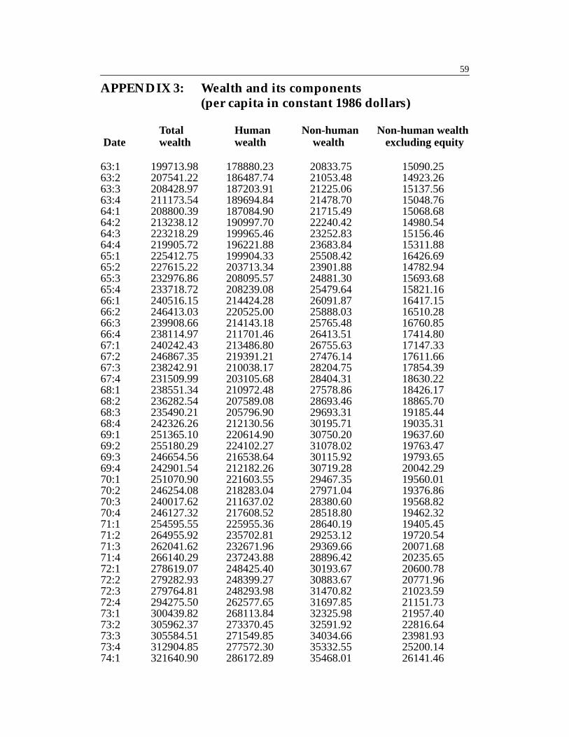
59

APPENDIX 3: Wealth and its components(per capita in constant 1986 dollars)

Total Human Non-human Non-human wealth Date wealth wealth wealth excluding equity

63:1 199713.98 178880.23 20833.75 15090.2563:2 207541.22 186487.74 21053.48 14923.2663:3 208428.97 187203.91 21225.06 15137.5663:4 211173.54 189694.84 21478.70 15048.7664:1 208800.39 187084.90 21715.49 15068.6864:2 213238.12 190997.70 22240.42 14980.5464:3 223218.29 199965.46 23252.83 15156.4664:4 219905.72 196221.88 23683.84 15311.8865:1 225412.75 199904.33 25508.42 16426.6965:2 227615.22 203713.34 23901.88 14782.9465:3 232976.86 208095.57 24881.30 15693.6865:4 233718.72 208239.08 25479.64 15821.1666:1 240516.15 214424.28 26091.87 16417.1566:2 246413.03 220525.00 25888.03 16510.2866:3 239908.66 214143.18 25765.48 16760.8566:4 238114.97 211701.46 26413.51 17414.8067:1 240242.43 213486.80 26755.63 17147.3367:2 246867.35 219391.21 27476.14 17611.6667:3 238242.91 210038.17 28204.75 17854.3967:4 231509.99 203105.68 28404.31 18630.2268:1 238551.34 210972.48 27578.86 18426.1768:2 236282.54 207589.08 28693.46 18865.7068:3 235490.21 205796.90 29693.31 19185.4468:4 242326.26 212130.56 30195.71 19035.3169:1 251365.10 220614.90 30750.20 19637.6069:2 255180.29 224102.27 31078.02 19763.4769:3 246654.56 216538.64 30115.92 19793.6569:4 242901.54 212182.26 30719.28 20042.2970:1 251070.90 221603.55 29467.35 19560.0170:2 246254.08 218283.04 27971.04 19376.8670:3 240017.62 211637.02 28380.60 19568.8270:4 246127.32 217608.52 28518.80 19462.3271:1 254595.55 225955.36 28640.19 19405.4571:2 264955.92 235702.81 29253.12 19720.5471:3 262041.62 232671.96 29369.66 20071.6871:4 266140.29 237243.88 28896.42 20235.6572:1 278619.07 248425.40 30193.67 20600.7872:2 279282.93 248399.27 30883.67 20771.9672:3 279764.81 248293.98 31470.82 21023.5972:4 294275.50 262577.65 31697.85 21151.7373:1 300439.82 268113.84 32325.98 21957.4073:2 305962.37 273370.45 32591.92 22816.6473:3 305584.51 271549.85 34034.66 23981.9373:4 312904.85 277572.30 35332.55 25200.1474:1 321640.90 286172.89 35468.01 26141.46

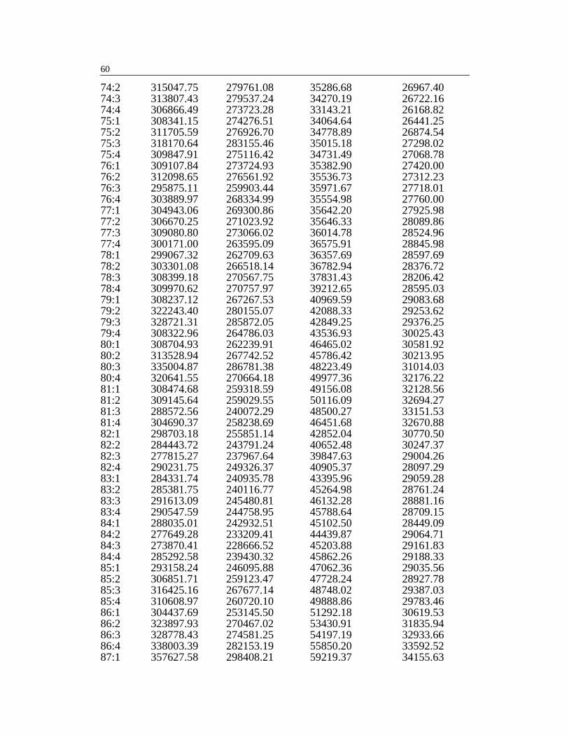
60

74:2 315047.75 279761.08 35286.68 26967.4074:3 313807.43 279537.24 34270.19 26722.1674:4 306866.49 273723.28 33143.21 26168.8275:1 308341.15 274276.51 34064.64 26441.2575:2 311705.59 276926.70 34778.89 26874.5475:3 318170.64 283155.46 35015.18 27298.0275:4 309847.91 275116.42 34731.49 27068.7876:1 309107.84 273724.93 35382.90 27420.0076:2 312098.65 276561.92 35536.73 27312.2376:3 295875.11 259903.44 35971.67 27718.0176:4 303889.97 268334.99 35554.98 27760.0077:1 304943.06 269300.86 35642.20 27925.9877:2 306670.25 271023.92 35646.33 28089.8677:3 309080.80 273066.02 36014.78 28524.9677:4 300171.00 263595.09 36575.91 28845.9878:1 299067.32 262709.63 36357.69 28597.6978:2 303301.08 266518.14 36782.94 28376.7278:3 308399.18 270567.75 37831.43 28206.4278:4 309970.62 270757.97 39212.65 28595.0379:1 308237.12 267267.53 40969.59 29083.6879:2 322243.40 280155.07 42088.33 29253.6279:3 328721.31 285872.05 42849.25 29376.2579:4 308322.96 264786.03 43536.93 30025.4380:1 308704.93 262239.91 46465.02 30581.9280:2 313528.94 267742.52 45786.42 30213.9580:3 335004.87 286781.38 48223.49 31014.0380:4 320641.55 270664.18 49977.36 32176.2281:1 308474.68 259318.59 49156.08 32128.5681:2 309145.64 259029.55 50116.09 32694.2781:3 288572.56 240072.29 48500.27 33151.5381:4 304690.37 258238.69 46451.68 32670.8882:1 298703.18 255851.14 42852.04 30770.5082:2 284443.72 243791.24 40652.48 30247.3782:3 277815.27 237967.64 39847.63 29004.2682:4 290231.75 249326.37 40905.37 28097.2983:1 284331.74 240935.78 43395.96 29059.2883:2 285381.75 240116.77 45264.98 28761.2483:3 291613.09 245480.81 46132.28 28881.1683:4 290547.59 244758.95 45788.64 28709.1584:1 288035.01 242932.51 45102.50 28449.0984:2 277649.28 233209.41 44439.87 29064.7184:3 273870.41 228666.52 45203.88 29161.8384:4 285292.58 239430.32 45862.26 29188.3385:1 293158.24 246095.88 47062.36 29035.5685:2 306851.71 259123.47 47728.24 28927.7885:3 316425.16 267677.14 48748.02 29387.0385:4 310608.97 260720.10 49888.86 29783.4686:1 304437.69 253145.50 51292.18 30619.5386:2 323897.93 270467.02 53430.91 31835.9486:3 328778.43 274581.25 54197.19 32933.6686:4 338003.39 282153.19 55850.20 33592.5287:1 357627.58 298408.21 59219.37 34155.63

61

87:2 356297.31 295864.21 60433.10 34653.2187:3 350484.23 287102.30 63381.92 35340.3987:4 351493.12 293623.24 57869.88 36140.6888:1 362271.41 303096.20 59175.21 37361.8988:2 355871.15 294741.20 61129.95 38568.6088:3 356962.94 294831.17 62131.77 39711.0388:4 363093.31 298708.11 64385.20 41362.4489:1 359172.46 291311.83 67860.63 44095.7589:2 352292.81 286731.84 65560.97 41708.2289:3 359725.54 290878.09 68847.45 43323.6889:4 351797.83 281352.02 70445.81 44452.8890:1 343077.84 275980.88 67096.96 43556.1690:2 339563.46 275123.85 64439.62 42423.7390:3 337919.27 274018.82 63900.45 42930.0690:4 335291.15 273184.94 62106.21 41894.6591:1 347347.21 283589.50 63757.71 42359.8991:2 347803.07 282722.90 65080.17 43293.5591:3 339077.59 275786.95 63290.64 41652.1691:4 340602.75 277153.79 63448.96 40976.9592:1 343385.90 280678.60 62707.30 40417.5492:2 348329.90 286640.59 61689.32 40394.8492:3 346892.35 284791.78 62100.56 40694.7392:4 342518.68 280058.66 62460.01 40948.4693:1 348262.22 286535.98 61726.24 39918.6493:2 351924.72 287575.41 64349.30 39866.6993:3 354835.65 289673.15 65162.50 39539.28

63

BIBLIOGRAPHY

Andrews, D. W. K. 1990. “Tests for Parameter Instability and StructuralChange with Unknown Change Point.” Discussion Paper No. 943.Cowles Foundation for Research in Economics, Yale University,New Haven.

––––––––––. 1991. “Heteroskedasticity and Autocorrelation ConsistentCovariance Matrix Estimation.” Econometrica 59:817–58.

Beach, C. M., R. W. Boadway and N. Bruce. 1988. “Taxation and Savings inCanada.” Technical paper prepared for the Economic Council ofCanada.

Campbell, J. Y. 1987. “Does Saving Anticipate Declining Labor Income?:An Alternative Test of the Permanent Income Hypothesis.”Econometrica 55:1249–73.

Campbell, J. Y. and N. G. Mankiw. 1990. “Permanent Income, CurrentIncome, and Consumption.” Journal of Business & Economic Statistics

8:265–79.

Davidson, J. E. H. and D. F. Hendry. 1981. “Interpreting EconometricEvidence: The Behaviour of Consumers’ Expenditure in the UK.”European Economic Review 16:177–92.

Davidson, J. E. H., D. F. Hendry, F. Srba and S. Yeo. 1978. “EconometricModelling of the Aggregate Time-Series Relationship Between Con-sumers’ Expenditure and Income in the United Kingdom.” The

Economic Journal 88:661–92.

Dickey, D. A. and W. A. Fuller. 1979. “Distribution of the Estimators forAutoregressive Time Series with a Unit Root.” Journal of the Ameri-

can Statistical Association 74:427–31.

Engle, R. F. and C. W. J. Granger. 1987. “Co-integration and Error Correc-tion: Representation, Estimation and Testing.” Econometrica 55:251–76.

64

Flavin, M. A. 1981. “The Adjustment of Consumption to ChangingExpectations About Future Income.” Journal of Political Economy 89:974–1009.

––––––––––. 1985. “Excess Sensitivity of Consumption to Current Income:Liquidity Constraints or Myopia?” Canadian Journal of Economics 18:117–36.

Gregory, A. W. 1991. “Testing for Cointegration in Linear QuadraticModels.” Working Paper 811. Queen’s University, Kingston (ON).

Hall, A. 1989. “Testing for a Unit Root in the Presence of Moving AverageErrors.” Biometrika 76:49–56.

Hall, R. E. 1978. “Stochastic Implications of the Life Cycle–PermanentIncome Hypothesis: Theory and Evidence.” Journal of Political

Economy 86:971–87.

Hall, R. E. and F. S. Mishkin. 1982. “The Sensitivity of Consumption toTransitory Income: Estimates from Panel Data on Households.”Econometrica 50:461–81.

Hansen, B. E. 1992. “Tests for Parameter Instability in Regressions with I(1)Processes.” Journal of Business & Economic Statistics 10:321–35.

Harnett, I. R. 1988. “An Error Correction Model of U.S. ConsumptionExpenditures.” Discussion Paper No. 34. Bank of England, London.

Haug, A. A. 1992. “Critical Values for the -Phillips-Ouliaris Test forCointegration.” Oxford Bulletin of Economics and Statistics 54:473–80.

Hayashi, F. 1982. “The Permanent Income Hypothesis: Estimation andTesting by Instrumental Variables.” Journal of Political Economy

90:895–916.

Hendry, D. F. and J. F. Richard. 1982. “On the Formulation of EmpiricalModels in Dynamic Econometrics.” Journal of Econometrics 20:3–33.

Zα

65

Hendry, D. F. and T. von Ungern-Sternberg. 1981. “Liquidity and InflationEffects on Consumer’s Expenditure.” In Essays in the Theory and

Measurement of Consumer Behaviour, edited by A. Deaton, 237–60.Cambridge (England): Cambridge University Press.

Irvine, I. J. 1980. “The Distribution of Income and Wealth in Canada in aLifecycle Framework.” Canadian Journal of Economics 13:455–74.

Jarque, C. M. and A. K. Bera. 1980. “Efficient Test for Normality, Homo-scedasticity and Serial Independence of Regression Residuals.”Economics Letters 6:255–59.

MacKinnon, J. G. 1991. “Critical Values for Cointegration Tests.” In Long-

Run Economic Relationships: Readings in Cointegration, edited byR. F. Engle and C. W. J. Granger, 267–76. New York: Oxford Univer-sity Press.

Macklem, R. T. 1991. “A Flexible, Forward-Looking Measure of Wealth.”Working Paper 91–5. Bank of Canada, Ottawa.

Mankiw, N. G. and S. P. Zeldes. 1990. “The Consumption of Stockholdersand Non-Stockholders.” Working Paper 3402. National Bureau ofEconomic Research, Cambridge (MA).

Michener, Ron. 1984. “Permanent Income in General Equilibrium.” Journal

of Monetary Economics 13:297–305.

Nelson, C. R. 1987. “A Reappraisal of Recent Tests of the PermanentIncome Hypothesis.” Journal of Political Economy 95:641–46.

Newey, W. K. and K. D. West. 1987. “A Simple, Positive Semi-Definite Het-eroscedasticity and Autocorrelation Consistent Covariance Matrix.”Econometrica 55:703–8.

Patterson, K. D. 1991. “An Error Correction System for Integrated Con-sumption and Portfolio Allocation Decisions.” Economics Letters

35:111–16.

66

Perron, P. 1991. “Test Consistency with Varying Sampling Frequency.”Econometric Theory 7:341–68.

Phillips, P. C. B. and B. E. Hansen. 1990. “Statistical Inference in Instrumen-tal Variables Regression with I(1) Processes.” Review of Economic

Studies 57:99-125.

Phillips, P. C. B. and S. Ouliaris. 1990. “Asymptotic Properties of ResidualBased Tests for Cointegration.” Econometrica 58:165–93.

Phillips, P. C. B. and P. Perron. 1988. “Testing for a Unit Root in Time SeriesRegression.” Biometrika 75:335–46.

Poloz, S. S. 1986. An Integrated Model of the Portfolio Behaviour of the Canadian

Household Sector: 1968–1983. Technical Report No. 41. Ottawa: Bankof Canada.

Rose, D. E. and J. G. Selody. 1985. The Structure of the Small Annual Model.Technical Report No. 40. Ottawa: Bank of Canada.

Rossi, N. and F. Schiantarelli. 1982. “Modelling Consumers’ Expenditure:Italy, 1965–1977.” European Economic Review 17:371–91.

Said, S. E. and D. A. Dickey. 1984. “Testing for Unit Roots inAutoregressive-Moving Average Models of Unknown Order.”Biometrika 71:599–608.

Sawyer, J. A. 1991. “Trends, Unit Roots, Cointegration, and Error Correc-tion Mechanisms: A Literature Summary and an ECM ConsumptionFunction.” Technical Study 91–1. Institute for Policy Analysis,University of Toronto.

Schwert, G. W. 1987. “Effects of Model Specification on Tests for Unit Rootsin Macroeconomic Data.” Journal of Monetary Economics 20:73–103.

Steel, M. F. J. 1987. “Testing for Exogeneity: An Application to ConsumerBehaviour.” European Economic Review 31:1443–63.

67

Stock, J. H. and M. W. Watson. 1993. “A Simple Estimator of CointegratingVectors in Higher Order Integrated Systems.” Econometrica 61:783–820.

Tauchen, G. 1986. “Finite State Markov-Chain Approximations to Univari-ate and Vector Autoregressions.” Economics Letters 20:177–81.

Thury, G. 1989. “Dynamic Specification of Consumer Expenditure on Non-Durables and Services in Austria.” Empirica 16:67–83.

Wirjanto, T. S. 1991. “Testing the Permanent Income Hypothesis: TheEvidence from Canadian Data. Canadian Journal of Economics 24:563–77.

Zeldes, S. P. 1989. “Consumption and Liquidity Constraints: An EmpiricalInvestigation.” Journal of Political Economy 97:305–46.