weakly supervised scale-invariant learning of …fergus/papers/fergus_ijcv.pdfweakly supervised...

Weakly Supervised Scale-Invariant Learning of Models for VisualRecognition

R. Fergus1 P. Perona2 A. Zisserman1

1 Dept. of Engineering Science 2 Dept. of Electrical EngineeringUniversity of Oxford California Institute of TechnologyParks Road, Oxford MC 136-93, Pasadena

OX1 3PJ, U.K. CA 91125, U.S.A.

{fergus,az}@robots.ox.ac.uk [email protected]

July 19, 2005

Abstract

We investigate a method for learning object categories in a weakly supervised manner. Given a set of

images known to contain the target category from a similar viewpoint, learning is translation and scale-

invariant; does not require alignment or correspondence between the training images, and is robust

to clutter and occlusion. Category models are probabilistic constellations of parts, and their parame-

ters are estimated by maximizing the likelihood of the training data. The appearance of the parts, as

well as their mutual position, relative scale and probability of detection are explicitly described in the

model. Recognition takes place in two stages. First, a feature-finder identifies promising locations for the

model’s parts. Second, the category model is used to compare the likelihood that the observed features

are generated by the category model, or are generated by background clutter. The flexible nature of the

model is demonstrated by results over six diverse object categories including geometrically constrained

categories (e.g. faces, cars) and flexible objects (such as animals).

1

Motorbikes Airplanes Faces Cars (Side) Cars (Rear) Spotted Cats

Caltech

Background

Google

Background

Figure 1: Some sample images from the datasets. Note the large variation in scale in, for ex-ample, the cars (rear) database. These datasets are from both http://www.vision.caltech.edu/html-files/archive.html and http://www.robots.ox.ac.uk/∼vgg/data/, except for the Cars (Side) from(http://l2r.cs.uiuc.edu/∼cogcomp/index research.html) and Spotted Cats from the Corel Image library. A Power-point presentation of the figures in this paper can be found at http://www.robots.ox.ac.uk/∼vgg/presentations.html

2

1 Introduction

Representation, detection and learning are the main issues that need to be tackled in designing a visual

system for recognizing object categories. The first challenge is coming up with models that can capture

the ‘essence’ of a category, i.e. what is common to the objects that belong to it, and yet are flexible

enough to accommodate object variability (e.g. presence/absence of distinctive parts such as mustache

and glasses, variability in overall shape, changing appearance due to lighting conditions, viewpoint etc).

The challenge of detection is defining metrics and inventing algorithms that are suitable for matching

models to images efficiently in the presence of occlusion and clutter. Learning is the ultimate challenge.

If we wish to be able to design visual systems that can recognize, say, 10,000 object categories, then

effortless learning is a crucial step. This means that those training steps that require a human operator

(e.g. collection of good quality training exemplars of the category; elimination of clutter; correspondence

and scale normalization of the training examples) should be reduced to a minimum or eliminated.

In this paper we develop and discuss a probabilistic model for an object category which can be learnt

from a set of training images of instances of that category, requiring only weak supervision. The model

represents a single visual aspect of the object category (e.g. the side view of a car) and accommodates

intra-category variability. The training images are required to contain a single instance of the category

with a common visual aspect and orientation. These requirements are the extent of the weak supervision.

The instances do not need to be aligned (e.g. centred) or scale normalized or put in correspondence, and

the images may contain clutter (i.e. foreground segmentation is not required).

Object recognition dates back to the origin of the computer vision field. However, for the most part

the emphasis has been on efficiently recognizing single 2D or 3D object instances (e.g. a particular sta-

pler) [28] rather than an object category (all types of staplers) under unrestricted viewpoints. A number

of successful approaches — geometric alignment, geometric hashing, appearance manifolds etc — have

been developed with objects being represented by their wireframe outline or internal appearance, and

viewpoint mappings ranging from 2D transformations (e.g. affinities), through parallel projection (affine

cameras) to the full generality of perspective projection. This progress is covered in text books such

as [16].

3

However, the emphasis in this paper is not on viewpoint invariance, indeed learning is restricted to

scale and translation invariance, but on modelling and learning intra-category variability. A number of

recent papers have also tackled this problem. A key issue is how to represent an object category. One

popular approach is to model categories as a collection of features, or parts, each part having a distinctive

appearance and (in most cases) spatial position [2, 3, 4, 5, 7, 10, 19, 21, 25, 33, 34, 37, 38, 43]. Different

authors vary widely on the details: the number of parts they envisage (from a few to thousands of parts),

how these parts are detected and represented, how their position is represented, whether the variability

in part appearance and position is represented explicitly or is implicit in the details of the matching

algorithm. The issue of learning is perhaps the least well understood. Most authors rely on manual steps

to eliminate background clutter and normalize the pose of the training examples. Recognition can also

proceed by an exhaustive search over image position and scale [24, 32, 34, 36, 38, 39].

We focus our attention on the probabilistic approach proposed by Burl et al. [5] which models objects

as random constellations of parts. This approach presents several advantages: the model explicitly ac-

counts for shape variations and for the randomness in the presence/absence of features due to occlusion

and detector errors. It accounts explicitly for image clutter. It yields principled and efficient detection

methods. Weber et al. [42, 43] proposed a maximum likelihood weakly supervised learning algorithm for

the “constellation model” which successfully learns object categories in a translation invariant manner

from cluttered data with minimal human intervention. We propose here four substantial improvements

to the constellation model and to its maximum likelihood learning algorithm. First, while Burl et al.

and Weber et al. model explicitly shape variability, they do not model the variability of appearance. We

extend their model to take this aspect into account. Second, appearance here is learnt simultaneously

with shape, whereas in their work the appearance of a part is fixed before shape learning. Third, they

use correlation to detect their parts. We substitute their front end with an interest operator, which detects

regions and their scale in the manner of [27, 30]. Fourth, Weber et al. did not experiment extensively

with scale-invariant learning, most of their training sets are collected in such a way that the scale is ap-

proximately normalized. We extend their learning algorithm so that new object categories may be learnt

efficiently, without supervision, from training sets where the object examples have large variability in

scale. A final contribution is experimenting with a number of new image datasets to validate the overall

4

approach over several object categories. Examples images from these datasets are shown in Figure 1.

The aim of this paper is to describe our probabilistic object model and learning algorithm in sufficient

detail to make implementation possible, as well as giving an insight into its design. In section 2 we give

the structure of the model and describe our region detector. In section 3 we show how to estimate

the parameters of our model, given a set of training images. Section 4 describes the use of the model in

recognition. Our approach is then tested on a wide variety of data in section 5. Experiments investigating

our algorithm’s operation are also performed, including the sensitivity of parameter settings and the

importance of different components within the model. Finally, conclusions are drawn in section 6.

2 Model structure

Our approach to modeling object categories follows on from the work of Burl et al. and Weber et al.

[5, 40, 42, 43]. An object model consists of a number of parts. Each part has an appearance, relative

scale and can be occluded or not. Each part has a certain probability of being erroneously detected in the

background clutter. Shape is represented by the mutual position of the parts. The entire model is gener-

ative and probabilistic, so appearance, scale, shape and occlusion are all modeled by probability density

functions, which here are Gaussians. The model is scale and translation invariant in both learning and

recognition. The process of learning an object category is one of first detecting regions and their scales,

and then estimating the parameters of the above densities from these regions, such that the model gives

a maximum-likelihood description of the training data. Recognition is performed on a query image by

again first detecting regions and their scales, and then evaluating the regions using the model parameters

estimated in the learning. Note that parts refer to the model, while features refer to detections in the

image.

The model is best explained by first considering recognition. Assume, we have learnt a generative

object category model, with P parts and parameters θfg. We also assume that all non-object images can

be modeled by a background with a single, fixed, set of parameters θbg. We are then presented with a new

image and we must decide if it contains an instance of our object category or not. In this query image we

have identified N interesting features with locations X, scales S, and appearances A. We now make a

decision as to the presence/absence of the object by comparing the ratio of category posterior densities,

5

R, to a threshold T :

R =p(Object|X,S,A)

p(No object|X,S,A)=

p(X,S,A|Object) p(Object)p(X,S,A|No object) p(No object) ≈

p(X,S,A| θfg) p(Object)p(X,S,A|θbg) p(No object) (1)

The last expression is an approximation since we represent the category with its (imperfect) model,

parameterized by θ. The ratio of the priors may be estimated from the training set or set by hand (usually

to 1).

Since our model only has P (typically 3-7) parts but there are N (up to 30) features in the image, we

use an indexing variable h (as introduced in [5]) which we call a hypothesis. h is a vector of length P ,

where each entry is between 0 and N which allocates a particular feature to a model part. The unallocated

features are assumed to be part of the background, with 0 indicating the part is unavailable (e.g. because

of occlusion). The set H is all valid allocations of features to the parts; consequently |H| is O(N P ).

Computing R in (1) requires the calculation of the ratio of the two likelihood functions. In order to do

this, the likelihoods are factored as follows:

p(X,S,A| θfg) =∑

h∈H

p(X,S,A,h| θfg) =∑

h∈H

p(A|X,S,h, θfg)︸︷︷︸

Appearance

p(X|S,h, θfg)︸︷︷︸

Shape

p(S|h, θfg)︸︷︷︸

Rel. Scale

p(h|θfg)︸︷︷︸

Other

(2)

We now look at each of the likelihood terms and derive their actual form. The likelihood terms model

not only the properties of the features assigned to the models parts (the foreground) but also the statistics

of features in the background of the image (those not picked out by the hypothesis). Therefore it will

be helpful to define the following notation: d = sign(h) (which is a binary vector giving the state of

occlusion for each part, i.e. dp = 1 if part p is present and dp = 0 if absent), nfg = sum(d) (the number

of foreground features under the current hypothesis) and nbg = N − nfg (the number of background

features).

If we believe no object to be present, then all features in the image belong to the background. Thus we

only have one possible hypothesis: h0 = 0, the null hypothesis. So the likelihood in this case becomes:

p(X,S,A| θbg) = p(A|X,S,h0, θbg)p(X|S,h0, θbg)p(S|h0, θbg)p(h0|θbg) (3)

As we will see below, p(X,S,A| θbg) is a constant for a given image. This simplifies the computation of

the likelihood ratio in (1), since p(X,S,A| θbg) can be moved inside the summation over all hypotheses

in (2), to cancel with the foreground terms.

6

2.1 Appearance

Here we describe the form of p(A|X,S,h, θ) which is the appearance term of the object likelihood.

We simplify the expression to p(A|h, θ) since given the detected features, we assume their appearance

and location to be independent. Each feature’s appearance is represented as a point in an appearance

space, defined below. Each part p has a Gaussian density within this space, with mean and covariance

parameters θappfg,p = {cp, Vp} which is independent of other parts’ densities. The background model has

fixed parameters θappbg = {cbg, Vbg}. Both Vp and Vbg are assumed to be diagonal. The appearance density

is computed over all features: each feature selected by the hypothesis is evaluated under the appropriate

part density while all features not selected by the hypothesis are evaluated under the background density:

p(A|h, θfg) =P∏

p=1

G(A(hp)|cp, Vp)dp

N∏

j=1,j\h

G(A(j)|cbg, Vbg) (4)

where G is the Gaussian distribution. A(hp) is the appearance of the feature picked by hp. If no object

is present, then all features are evaluated under the background density:

p(A|h0, θbg) =N∏

j=1

G(A(j)|cbg, Vbg) (5)

As p(A|h0, θbg) is a constant and so is not dependent on h, so we can cancel terms between (4) and (5)

when computing the likelihood ratio in (1):

p(A|h, θfg)

p(A|h, θbg)=

P∏

p=1

(G(A(hp)|cp, Vp)

G(A(hp)|cbg, Vbg)

)dp

(6)

So the appearance of each feature in the hypothesis is evaluated under foreground and background den-

sities and the ratio taken. If the part is occluded, the ratio is 1 (dp = 0).

This term is an addition to the previous incarnations of the constellation model in Weber et al. and

Burl et al. [5, 43].

2.2 Shape

Here we describe the form of p(X|S,h, θ) which is the shape term of the object likelihood. The shape

of the object is represented by a joint Gaussian density of the locations of features within a hypothesis,

once they have been transformed into a scale and translation-invariant space. This representation allows

7

the modeling of both inter and intra part variability: interactions between the parts (both attractive and

repulsive) as well as uncertainty in location of the part itself.

Translation invariance is achieved by using the location of the feature assigned to the first non-

occluded part as a landmark. We then model the shape of the remaining features in the hypothesis

relative to this landmark feature. Scale invariance is achieved by using the scale of the landmark part

to normalize the locations of the other features in the constellation. This approach avoids an exhaustive

search over scale that other methods use. If the index of the first non-occluded part is l, then the landmark

feature’s location is X(hl) and its scale is S(hl).

X(h) is a 2P vector holding the x and y coordinates of each feature in hypothesis h, i.e.

X(h) = {xh1, . . . , xhP

, yh1, . . . , yhP

} . To obtain translation invariance, we subtract the location of the

landmark from X(h): X∗(h) = {xh1

− xhl, . . . , xhP

− xhl, yh1

− yhl, . . . , yhP

− yhl}. A scale invariant

representation is obtained by dividing through by S(hl): X∗∗(h) = X∗(h)

S(hl). Note that ∗ indicates a repre-

sentation that is translation invariant, while ∗∗ denotes a representation that is both scale and translation

invariant.

We model X∗∗(h) with a Gaussian density which has parameters θshapefg = {µ, Σ}. Since any of the P

parts can act as the landmark, µ, Σ consist of a set of P µl’s and Σl’s to evaluate X∗∗(h) with. However,

the set members are equivalent to one another since changing landmark just involves a translation of µ

and the equivalent transformation of Σ (a referral of variances between the old and new landmark), due

to the properties of Gaussian distributions.

Due to translation invariance, µl is a 2(P − 1) vector (x and y coordinates of the non-landmark

parts). Correspondingly, Σl is a 2(P − 1) by 2(P − 1) matrix. Note that, unlike appearance whose

covariance matrices Vp, Vbg are diagonal, Σl is a full matrix. All features not included in the hypothesis

are considered as arising from the background. The model for the background assumes features to

be spread uniformly over the image (which has area α), with locations independent of the foreground

locations. We also assume that the landmark feature can occur anywhere in the image, so its location is

modeled by a uniform density of 1/α.

p(X|S,h, θfg) =

(1

αG(X∗∗(h)|µl, Σl)

)(1

α

)nbg

(7)

If a part is occluded then we marginalize it out, which for a Gaussian entails deleting the appropriate

8

dimensions from the mean and covariance matrix. See [40] for more details.

If no object is present, then all detections are in the background and are consequently modeled by a

uniform distribution:

p(X|S,h0, θbg) =

(1

α

)N

(8)

Again, this is a constant, so we can cancel between (7) and (8) for the likelihood ratio in (1) to give:

p(X|S,h, θfg)

p(X|S,h0, θbg)= G(X∗∗(h)|µl, Σl) αnfg−1 (9)

This term is similar in nature to the shape term in [43], with the additional use of scale information

from the features to obtain scale-invariance. Leung et. al. [26] proposed an affine invariant shape repre-

sentation by the use of three model parts as a basis, transforming density of the remaining model parts

into a Dryden-Mardia density [29]. The complex nature of this density restricts its use to recognition,

hence learning must be performed manually. A requirement of our weakly supervised learning scheme is

that the transformed shape density is Gaussian, thus we are restricted to using one landmark only. In our

case, a feature only gives location and scale (i.e. not orientation), therefore we are currently restricted to

scale and translation invariance.

2.3 Relative scale

Here we describe the form of p(S|h, θ) which is the relative scale term of the object likelihood. This

term has the same structure as the shape term. The scale of parts relative to the scale of the landmark

feature is modeled by a Gaussian density in log space which has parameters θscalefg = {t, U}. Again, since

the landmark feature could belong to any of the P parts, these parameters are really a set of equivalent

tl, Ul’s. The parts are assumed to be independent of one another, thus Ul is a diagonal (P −1) by (P −1)

matrix, with tl being a (P − 1) vector. The background model assumes a uniform distribution over scale

(within a range r).

p(S|h, θfg) =

(1

rG(log S

∗(h)|tl, Ul)

)(1

r

)nbg

(10)

If the object is not present, all detections are modeled by the uniform distribution:

p(S|h0, θbg) =

(1

r

)N

(11)

9

Thus the ratio of likelihood becomes:

p(S|h, θfg)

p(S|h0, θbg)= G(log S

∗(h)|tl, Ul) rnfg−1 (12)

This term is an addition to the previous incarnations of the Constellation model of Weber et al. and

Burl et al. [5, 43].

2.4 Occlusion and Statistics of the feature finder

p(h|θfg) = pPoiss(nbg|M)1

nCr(N,nfg)p(d|D) (13)

The first term models the number of features in the background, using a Poisson distribution, which has

a mean M . The second is a book-keeping term for the hypothesis variable: we are picking nfg features

from a total of N and since we have no bias toward particular features, all combinations are equally

likely thus it is a constant for all h. The last term is a joint distribution on the occlusions of model parts.

It is a multinomial density (of size 2P ), modeling all possible occlusion patterns d, having a parameter,

D. This joint distribution allows the modeling of correlations in occlusion: nearby parts are more often

occluded together than far apart things. In the null case, we only have only possible hypothesis, h0, so

the only term from (13) that remains is the Poisson which now has to account for all features belonging

to the background:

p(h0|θbg) = pPoiss(N |M) (14)

Thus the ratio becomes:

p(h|θfg)

p(h|θbg)=

pPoiss(nbg|M)

pPoiss(N |M)

1nCr(N,nfg)

p(d|D) (15)

These terms were introduced by Weber et al. [43].

2.5 Model structure summary

The model encompasses many of the properties of an object, all in a probabilistic way, so this model

can represent both geometrically constrained objects (where the shape density would have a small co-

variance) and objects with distinctive appearance but lacking geometric form (the appearance densities

would be tight, but the shape density would now be looser). Some additional assumptions inherent in our

10

chosen model structure include: given a set of detected features, their appearance and location are inde-

pendent; the foreground features’ appearances are independent to one another; the background features’

are independent to the foreground and each other.

An important limitation of the model, as presented, is that we can only model one aspect of the

object. While this is a major limitation, many objects often appear in a distinctive pose (e.g. faces from

the front) thus single aspect recognition is still a worthwhile problem. More importantly, our approach

can be extended to multiple aspects by using a mixture of constellation models, in the manner of Weber

et al. [41].

Using (6),(9),(12) and (15) we can write the likelihood ratio from (1) as:

p(X,S,A|θfg)

p(X,S,A|θbg)=

∑

h∈H

p(X,S,A,h|θfg)

p(X,S,A,h0|θbg)(16)

=∑

h∈H

P∏

p=1

(G(A(hp)|cp, Vp)

G(A(hp)|cbg, Vbg)

)dp G(X∗∗(h)|µl, Σl) G(log S∗(h)|tl, Ul) (αr)nfg−1 pPoiss(nbg|M)p(d|D)

pPoiss(N |M) nCr(N,nfg)

The intuition is that the majority of the hypotheses will be low scoring as they will be picking up features

from background clutter on the image but hopefully a few features will genuinely be part of the object

and hypotheses using these will score highly. However, we must be able to locate features over many

different instances of the object and over a range of scales in order for this approach to work.

2.6 Feature detection

Features are found using the detector of Kadir and Brady [22]1. This method finds regions that are salient

over both location and scale. For each point in the image a histogram P (I) is made of the intensities

in a circular region of radius (scale) s. The entropy H(s) of this histogram is then calculated and the

local maxima of H(s) are candidate scales for the region. The saliency of each of these candidates is

measured by H dPds

(with appropriate normalization for scale [22, 27]).

This gives a 3-D saliency map (over x,y and s). Regions of high saliency are clustered over both

location and scale, with a bias toward clusters of large scale, since they tend to be more stable between

object instances. The centroids of the clusters then provide the features for learning and recognition,

their coordinates within the saliency map defining the centre and radius of each feature.1An implementation of this feature detector is available at http://www.robots.ox.ac.uk/∼timork/salscale.html

11

A good example illustrating the saliency principle is that of a bright circle on a dark background. If

the scale is too small then only the white circle is seen, and there is no extrema in entropy. There is an

entropy extrema when the scale is slightly larger than the radius of the bright circle, and thereafter the

entropy decreases as the scale increases.

In practice this method gives stable identification of features over a variety of sizes and copes well

with intra-category variability. The saliency measure is designed to be invariant to scaling, although

experimental tests show that this is not entirely the case due to aliasing and other effects. Note, only

monochrome information is used to detect and represent features. The performance of the algorithm is

dependent on finding good features from which to learn a model. The effect of different feature detector

settings is investigated in Section 5.

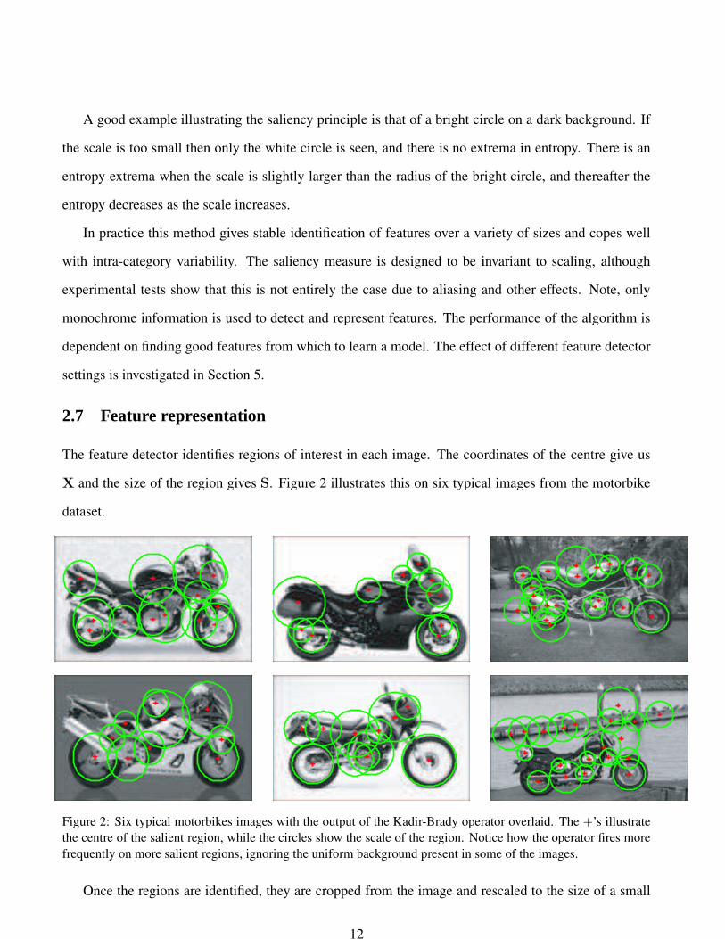
2.7 Feature representation

The feature detector identifies regions of interest in each image. The coordinates of the centre give us

X and the size of the region gives S. Figure 2 illustrates this on six typical images from the motorbike

dataset.

Figure 2: Six typical motorbikes images with the output of the Kadir-Brady operator overlaid. The +’s illustratethe centre of the salient region, while the circles show the scale of the region. Notice how the operator fires morefrequently on more salient regions, ignoring the uniform background present in some of the images.

Once the regions are identified, they are cropped from the image and rescaled to the size of a small

12

k × k patch (typically 11 ≤ k ≤ 21 pixels). Thus, each patch exists in a k2 dimensional space. Since

the appearance densities of the model must also exist in this space, we must somehow reduce the di-

mensionality of each patch whilst retaining its distinctiveness, since a 100+-dimensional Gaussian is

unmanageable from a numerical point of view and also the number of parameters involved (2k2 per

model part) are too many to be estimated.

This is done by using principal component analysis (PCA). We utilise three variants:

1. Intensity based PCA. The k × k patches are normalised to have zero mean and unit variance. This

is to remove the effects of lighting variation. They are then projected into a fixed PCA basis in the

intensity space of k × k patches, having l basis vectors. As used in Fergus et al. [14].

2. Gradient based PCA. Inspired by the performance of PCA-SIFT in region matching [23], we take

the x and y gradients of the k × k patch. The derivatives are computed by symmetric finite dif-

ference (cropping to avoid edge effects). The magnitude of the gradients within the patch is then

normalised to be 1, removing lighting variations. Note that we do not perform any orientation

normalization as in [23]. The outcome is a vector of length 2k2, with the first k elements repre-

senting the x derivative, and the second k the y derivatives. The normalized gradient-patch is then

projected into a fixed PCA basis of l dimensions.

3. Gradient based PCA with energy and residual. As for 2 but with two additional measurements

made for each gradient-patch: its unnormalized energy and the residual between the reconstructed

gradient-patch using the PCA basis and the original gradient-patch. Each region is thus represented

by a vector of length l + 2. The last two dimensions act as a crude interest measure of the region,

while the remaining dimensions actually represent its appearance.

Thus the appearance of each region is represented by a vector of PCA coefficients of length l or l + 2.

Combining the vectors from all regions we obtain A for an image.

The PCA basis is computed from patches extracted using all Kadir and Brady regions found on all

the training images of Motorbikes; Faces; Airplanes; Cars (Rear); Leopards and Caltech background.

Note that this basis is used for all object categories. We assume that the covariance terms between

components will be zero, thus Vp (the covariance of a part’s appearance) is diagonal in nature. Alternative

13

representations such as ICA and Fisher’s linear discriminant were also tried, but in experiments they were

shown to be inferior.

We have now computed X, S, and A for use in learning or recognition. For a typical image, this

takes 10-15 seconds (all timings given are for a 2 Ghz machine), mainly due to the unoptimized feature

detector. Optimization should reduce this to a few seconds.

3 Learning

In a weakly supervised learning scenario, one is presented with a collection of images containing ex-

amples of the objects amongst clutter. However the position and scale of the object with each image

is unknown; no correspondence between exemplars is given; parts of the object may be missing or oc-

cluded. The challenge is to make sense of this profusion of data. Weber et al.[43, 40] approached the

problem of weakly supervised learning of object categories in clutter as a maximum likelihood esti-

mation. For this purpose they derived an EM algorithm for the constellation model. We follow their

approach in deriving an EM algorithm to estimate the parameters of our improved model.

The task of learning is to estimate the parameters θfg = {µ, Σ, c, V,M,D, t, U} of the model dis-

cussed above. The goal is to find the parameters θML which best explain the data X,S,A from all

the training images, that is maximize the likelihood: θML = arg maxθ

p(X,S,A| θfg). Note that the

parameters of the background, θbg, are constant during learning.

Learning is carried out using the expectation-maximization (EM) algorithm [8] which iteratively

converges, from some random initial value of θfg to a maximum (which might be a local one).

We now look at each stage in the learning procedure, giving practical details of its implementation

and performance, using the motorbike dataset as an example. We assume that X,S,A have already been

extracted from the images, examples of which are shown in Figure 2. In this example, we are using the

gradient based PCA representation, with k = 11 and l = 15.

3.1 Initialization

Initially we have no knowledge about the structure of the object to be learnt so we are forced to initialize

the model parameters randomly. However, the model which has a large number of parameters, must be

14

initialized sensibly to ensure that the parameters will converge to a reasonable maximum. For shape, the

means are set randomly over the area of the image and the covariances to be large enough so that all

hypotheses have a roughly equal weighting, so avoiding a bias toward nearby points. The appearance

densities are initialised to zero mean, plus a small random perturbation, while the variances are set to

be large. The same initialization settings are used in all experiments. In Figure 3 we show three typical

model initializations of the shape term (the appearance term is hard to visualize due to the large number

of dimensions).

-150 -100 -50 0 50 100 150

150

100

50

0

-50

-100

-150

0.9

0.9

0.9

0.9

0.9

0.9

0.90.9

0.9

0.9

0.9

0.9

-150 -100 -50 0 50 100 150

150

100

50

0

-50

-100

-150

0.90.9

0.9

0.9

0.9

0.9

-150 -100 -50 0 50 100 150

150

100

50

0

-50

-100

-150

Figure 3: Three typical initializations for a 6 part motorbike shape model. The circles represent the variance ofeach part at 1 standard deviation (the inter-part covariance terms, which cannot easily be shown, are set to zero)with the mean being the centre of the circles. The probability of each part being present is shown just to the left ofthe mean. The average image size is indicated by the black box. As the images are resized to a constant width andtheir aspect ratio is unknown, we ensure that tall images are not penalised by allowing the initialization of some ofthe parts to lie outside the mean image box. Axis units are pixels. The variances here are referred to the centroidof the model.

3.2 EM update equations

The algorithm has two stages: (i) the E-step in which, given the current value of θfg at iteration k, θkfg,

some sufficient statistics are computed and (ii) the M-step where we compute the parameters for the next

iteration, θk+1fg using these sufficient statistics.

We now give the equations for both the E-step and M-step. The E-step requires us to compute the

posterior density of the hidden variables, which in our case are the hypotheses. This is calculated using

the joint:

p(h|X,S,A, θkfg) =

p(X,S,A,h| θkfg)

∑

h∈H p(X,S,A,h| θkfg)

=

p(X,S,A,h| θkfg

)

p(X,S,A,h0| θbg)

∑

h∈H

p(X,S,A,h| θkfg

)

p(X,S,A,h0| θbg)

(17)

15

We divide through by p(X,S,A,h0| θbg) as it is easier to compute the joint ratio rather than the joint

directly. We then calculate the following sufficient statistics for each image, i from which we have

previously extracted Xi,Ai,Si: E[X∗∗i], E[X∗∗i

X∗∗iT ], E[Ai

p], E[AipA

ip

T], E[S∗i], E[S∗i

S∗iT ], E[ni],

E[Di] where the expectation is taken with respect to the posterior, p(h|X,S,A, θkfg), for example:

E[X∗∗i] =∑

h∈H

p(h|Xi,Si,Ai, θkfg) X

∗∗i(h) (18)

Note that for simplicity we have not considered the case of missing data. The extensions to the above

rules for dealing with this may be found in [40]. The general principle is to condition on the features that

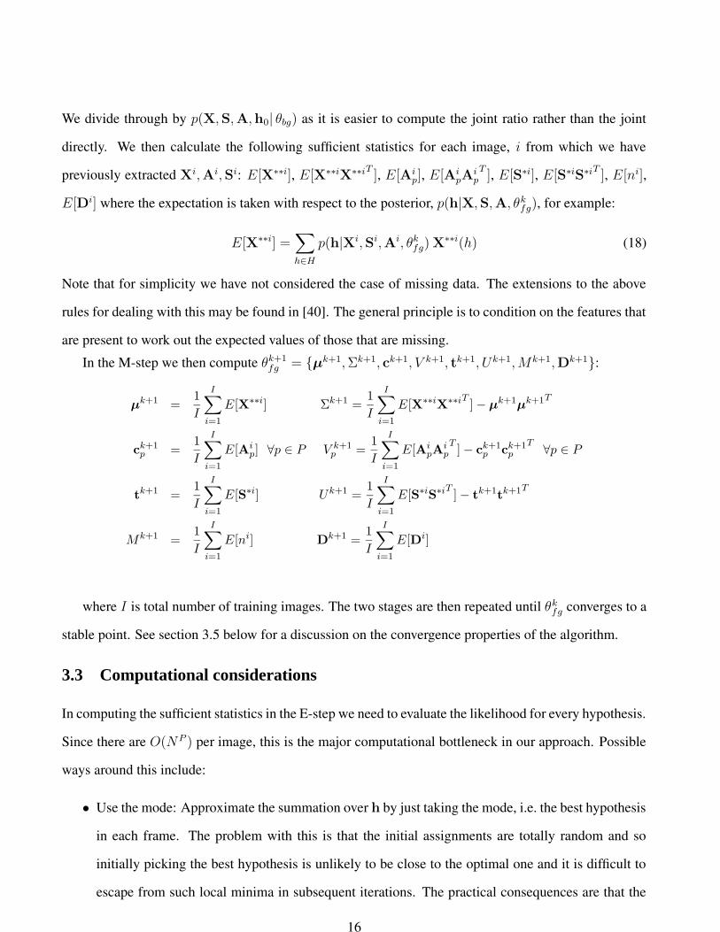
are present to work out the expected values of those that are missing.In the M-step we then compute θk+1

fg = {µk+1, Σk+1, ck+1, V k+1, tk+1, Uk+1,Mk+1,Dk+1}:

µk+1 =

1

I

I∑

i=1

E[X∗∗i] Σk+1 =1

I

I∑

i=1

E[X∗∗iX

∗∗iT ] − µk+1

µk+1T

ck+1p =

1

I

I∑

i=1

E[Aip] ∀p ∈ P V k+1

p =1

I

I∑

i=1

E[AipA

ip

T] − c

k+1p c

k+1p

T∀p ∈ P

tk+1 =

1

I

I∑

i=1

E[S∗i] Uk+1 =1

I

I∑

i=1

E[S∗iS∗iT ] − t

k+1tk+1T

Mk+1 =1

I

I∑

i=1

E[ni] Dk+1 =

1

I

I∑

i=1

E[Di]

where I is total number of training images. The two stages are then repeated until θkfg converges to a

stable point. See section 3.5 below for a discussion on the convergence properties of the algorithm.

3.3 Computational considerations

In computing the sufficient statistics in the E-step we need to evaluate the likelihood for every hypothesis.

Since there are O(NP ) per image, this is the major computational bottleneck in our approach. Possible

ways around this include:

• Use the mode: Approximate the summation over h by just taking the mode, i.e. the best hypothesis

in each frame. The problem with this is that the initial assignments are totally random and so

initially picking the best hypothesis is unlikely to be close to the optimal one and it is difficult to

escape from such local minima in subsequent iterations. The practical consequences are that the

16

model is more prone to numerical explosions (probabilities go to zero somewhere); or the models

converge to bad local maxima. See Figure 8(b) for an example of the latter.

• Sample hypotheses: While sampling methods could be used to evaluate the marginalization in the

E-step [20], the imposition of constraints (e.g. see Section 3.6) on possible hypotheses introduces

complications. These constraints mean that it would be more difficult to move through the space

of possible hypotheses, since many proposed moves would not be valid, increasing the chances of

hitting local minima. For this reason, we prefer more direct computation methods.

• Reduce the dependencies: The cause of our problems is assuming that the location of all parts is

dependent on one another. A simpler dependency structure could be adopted, conditioning on a

single landmark part, for example. This would reduce the O(N P ) problem to O(N 2P ). This is

investigated in [13].

• Efficient search methods: Only very small portion of the hypotheses have a high probability thus

we can accurately approximate the summation over all hypotheses by just considering this subset.

By utilizing various heuristics, specific to our application, we can efficiently compute the few

hypotheses contributing much of the probability mass. The details of this are now investigated in

Section 3.4.

3.4 Efficient search methods

Computing the very small portion of the hypotheses that have a high probability enables the learning

procedure to run in a reasonable time.

A tree structure is used to search the space of all possible hypotheses. The leaves of the tree are

complete hypotheses with each level representing a part: moving down the tree, features are allocated to

parts until a complete hypothesis is formed. At a node within the tree, an upper-bound on the probability

of remaining, unallocated parts can be computed enabling us to employ the A∗ algorithm [17, 18]. This

allows the efficient exploration of the tree, resulting in the guaranteed discovery of the best hypothesis.

This can be removed from the tree and the search continued until the next best hypothesis is found. In

this manner, we can extract the hypotheses ordered by likelihood. Figure 4(a) shows a toy example of

17

this process.

If q parts have been allocated, the upper bound on the probability for the remaining P − q parts

is easily computed thanks to the form of the densities in the model. Given the occlusion states of the

unallocated parts, the upper bound is a constant, thus it becomes a case of finding the maximum upper

bound for each of the 2P−q possible states.

A binary heap stores the list of open branches on the tree, having log n access time. Conditional

densities for each part (i.e. conditioning on previously allocated parts) are pre-computed to minimize the

computation necessary at each branch. Details of the A∗ search can be found in [15].

For each image, we compute all hypotheses until they become less than some threshold (e−15) smaller

than the best hypothesis. Figure 4(b) shows how the number of hypotheses varies for a given likelihood.

This threshold was chosen to ensure that the learning progressed within a reasonable time while evaluat-

ing as many hypotheses as possible. Additionally, space search methods are used to prune the branches

XX X

X0 X X1 X X2 X X3 X

01 X 21 X 31 X

21 0 21 3

Level 0: No parts allocated

Level 1: First part allocated

Level 2: First and second

parts allocated

Level 3: All parts allocated

Valid hypotheses

N = 3 detections

P = 3 parts

A=0

B=24

T=24

A=1

B=15

T=16

A=5

B=15

T=20

A=1

B=15

T=16

A=2

B=15

T=17

A=6

B=9

T=15

A=7

B=9

T=16

A=10

B=9

T=19

A=16

B=0

T=16

A=11

B=0

T=11

(a)

0 5 10 15 20 25 30 35 40 450

1

2

3

4

5

6x 104

Threshold (log10

)

Hyp

oth

esis

co

mp

ute

d

Iteration 1Iteration 5Iteration 40

(b)

0 5 10 15 20 25 30 35 40 450

1

2

3

4

5

6

7

Threshold (log10

)

Tim

e p

er

ima

ge

(se

cs)

Iteration 5Iteration 40Iteration 1

(c)

Figure 4: (a) Illustration of A∗ search process for a 3 part toy model and an image with 3 regions. As the tree isdescended, regions are allocated to parts, with the leaves of the tree constituting complete hypotheses. The score(T) of each node in the tree is a sum of the likelihood of the allocated features (A) and an upper-bound on thelikelihood of the remaining, unallocated features (B). The list of open nodes is stored in a binary heap, with thenode with the highest overall value (T) being the one opened next. By repeatedly removing complete nodes fromthe tree, the hypotheses can be extracted in order of likelihood. (b) A graph showing how the number of hypothesesevaluated increases as the likelihood drops below that of the best hypothesis on a typical motorbike model. Thevertical line shows the value of the threshold used in experiments. The three curves correspond to different stagesof learning: red – at the beginning when the model variances are large; green – in the middle and blue – when themodel variances are large (see Fig. 6(c) for evolution of model during learning). Note that as the model variancesdecrease, the number of hypotheses evaluted descreases. (c) As for (b), but the y-axis is evaluation time per image.

18

explored at each new node in the tree. At a given level of the tree, the joint density of the shape term

allows the density of location of the current part to be computed by conditioning on the previously al-

located parts. Only a subset of the N detections need be evaluated by this density: we assume that we

can neglect detections if their probability is worse than having all remaining parts be missing. Since the

occlusion probabilities are constant for a given learning iteration, this gives a threshold which truncates

the density. If the covariance of the density is small, only the best few detections need to be evaluated,

enabling significant numbers of hypotheses to be ignored.

Despite using these efficient methods, learning a P = 6–7 part model with N = 20–30 features per

image (a practical maximum), using 400 training images, takes around 24 hours to run. This equates to

spending 3-4 seconds per image, on average, at each iteration (given a total running time of 24 hours, with

400 training images and 50 EM iterations). It should be noted that learning only needs to be performed

once per category, due to the good convergence properties as discussed in section 3.5.

It is worth noting that just finding the best hypothesis (the mode), is not that much quicker than

taking the small subset of high scoring hypotheses (see Figure 4(c)), since a reasonable portion of the

tree structure must be explored before a complete hypothesis is found. This provides another justification

for summing over multiple hypotheses rather than just taking the best.

3.5 Convergence

Table 1 illustrates how the number of parameters in the model grows with the number of parts, (assuming

l = 15). Despite the large number of parameters in the model, its convergence properties are respectable.

Parts 2 3 4 5 6 7# parameters 77 123 177 243 329 451

Table 1: Relationship between number of parameters and number of parts in model

Figure 5 shows the convergence properties and classification performance of 15 models started from

different initial conditions but with identical data. Note that while the models converge at different rates

and to different points in parameter space (see the different shape models for each run in Figure 5(c)),the

ROC curves of test set performance are very similar, the standard deviation at equal-error rate being 0.6%.

Figure 6(a) shows the shape model evolving throughout the learning process for a typical learning run.

19

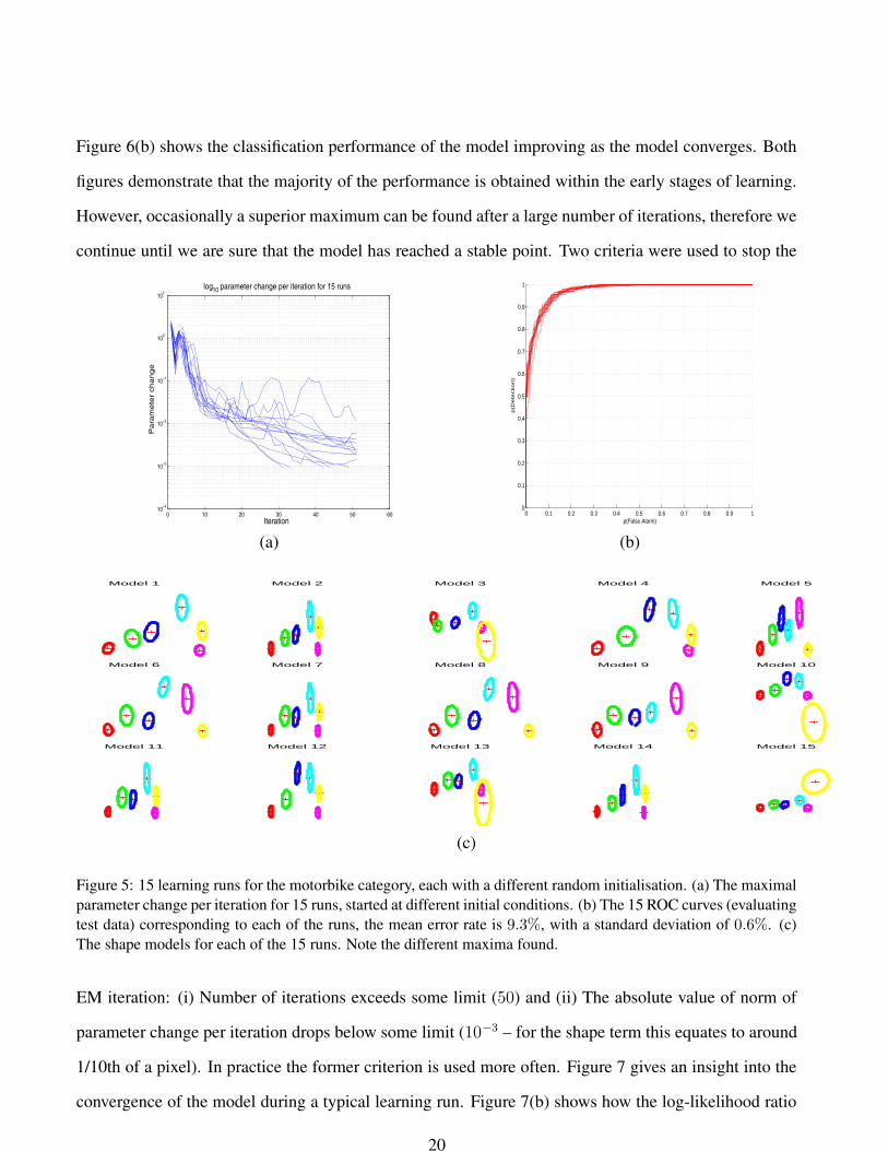
Figure 6(b) shows the classification performance of the model improving as the model converges. Both

figures demonstrate that the majority of the performance is obtained within the early stages of learning.

However, occasionally a superior maximum can be found after a large number of iterations, therefore we

continue until we are sure that the model has reached a stable point. Two criteria were used to stop the

0 10 20 30 40 50 6010

−4

10−3

10−2

10−1

100

101

Iteration

Pa

ram

ete

r ch

an

ge

log10 parameter change per iteration for 15 runs

(a)

0 0.1 0.2 0.3 0.4 0.5 0.6 0.7 0.8 0.9 10

0.1

0.2

0.3

0.4

0.5

0.6

0.7

0.8

0.9

1

p(False Alarm)p(D

ete

ction)

(b)

Model 1 Model 2 Model 3 Model 4 Model 5



(c)

Figure 5: 15 learning runs for the motorbike category, each with a different random initialisation. (a) The maximalparameter change per iteration for 15 runs, started at different initial conditions. (b) The 15 ROC curves (evaluatingtest data) corresponding to each of the runs, the mean error rate is 9.3%, with a standard deviation of 0.6%. (c)The shape models for each of the 15 runs. Note the different maxima found.

EM iteration: (i) Number of iterations exceeds some limit (50) and (ii) The absolute value of norm of

parameter change per iteration drops below some limit (10−3 – for the shape term this equates to around

1/10th of a pixel). In practice the former criterion is used more often. Figure 7 gives an insight into the

convergence of the model during a typical learning run. Figure 7(b) shows how the log-likelihood ratio

20

Start Model Iteration: 1 Iteration: 2 Iteration: 3

Iteration: 4 Iteration: 5 Iteration: 6 Iteration: 7

Iteration: 8 Iteration: 9 Iteration: 10 Final Model

(a)

0 5 10 15 20 25 30 35 40 450

0.05

0.1

0.15

0.2

0.25

0.3

0.35

0.4

0.45

0.5

Iteration

Err

or

rate

(%

)

TrainTest

0.87

0.991

1

0.9

0.42

(b)

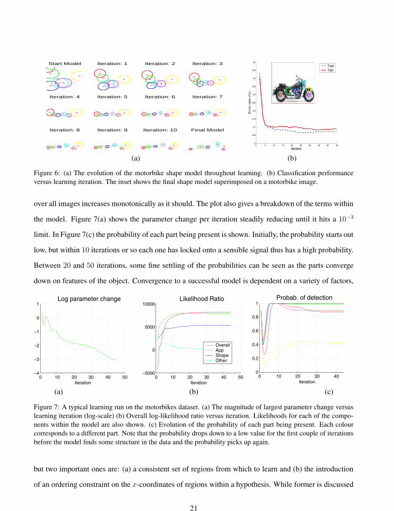
Figure 6: (a) The evolution of the motorbike shape model throughout learning. (b) Classification performanceversus learning iteration. The inset shows the final shape model superimposed on a motorbike image.

over all images increases monotonically as it should. The plot also gives a breakdown of the terms within

the model. Figure 7(a) shows the parameter change per iteration steadily reducing until it hits a 10−3

limit. In Figure 7(c) the probability of each part being present is shown. Initially, the probability starts out

low, but within 10 iterations or so each one has locked onto a sensible signal thus has a high probability.

Between 20 and 50 iterations, some fine settling of the probabilities can be seen as the parts converge

down on features of the object. Convergence to a successful model is dependent on a variety of factors,

0 10 20 30 400

0.2

0.4

0.6

0.8

1Probab. of detection

0 10 20 30 40 50−5000

0

5000

10000Likelihood Ratio

Iteration

0 10 20 30 40 50−4

−3

−2

−1

0

1Log parameter change

Iteration

OverallAppShapeOther

Iteration

(a) (b) (c)

Figure 7: A typical learning run on the motorbikes dataset. (a) The magnitude of largest parameter change versuslearning iteration (log-scale) (b) Overall log-likelihood ratio versus iteration. Likelihoods for each of the compo-nents within the model are also shown. (c) Evolution of the probability of each part being present. Each colourcorresponds to a different part. Note that the probability drops down to a low value for the first couple of iterationsbefore the model finds some structure in the data and the probability picks up again.

but two important ones are: (a) a consistent set of regions from which to learn and (b) the introduction

of an ordering constraint on the x-coordinates of regions within a hypothesis. While former is discussed

21

in more detail in Section 5.3.1, we now elaborate on the latter. To aid both convergence and speed, an

ordering constraint is placed on the x-coordinates of features allocated to parts: the features selected

must have a monotonically-increasing x-coordinate. This reduces the total number of hypotheses by P !

but unfortunately imposes an artificial constraint upon the shape of the object. If the object happens to

be orientated vertically then this constraint can exclude the best hypothesis. Clearly in this scenario,

imposing a constraint on the y-coordinate ordering would resolve the problem but it is not clear how to

choose such an appropriate constraint automatically, other than learning models with different ordering

constraints and picking the one with the highest likelihood. See Figure 8(a) for an example of a model

learnt without this constraint.

0.99

0.99

0.99

0.99

0.98

0.99

(a)

0.014

0.0092

110.981

(b)

0.87

0.99 1

1

0.9

0.42

(c)

Figure 8: (a) A motorbike shape model learnt using no ordering constraint on regions with hypotheses. Note thelarge overlapping distributions due to permutations of nearby features. The model is also P ! slower to learn thatthose with ordering constraints imposed. (b) A motorbike shape model learnt just using the best hypothesis ineach frame. A poor local maximum has been found with two parts being redundant, having a low probability ofoccurrence. (c) The shape model obtained if the an ordering constraint on the x-coordinates of the hypothesis isimposed.

3.6 Background model

Since the model is a generative one, the background images are not used in learning except for one

instance: the appearance model has a distribution in appearance space modeling background features.

Estimating this from foreground data proved inaccurate so the parameters were estimated from a set of

background images and not updated within the EM iteration.

3.7 Final model

In Figure 9 we show a complete model, from one of the 15 training runs on the motorbike dataset. It

is pleasing to see that a sensible spatial structure has been picked out and that the appearance samples

correspond to distinctive parts of the motorbike. In Figure 10 the appearance density of the model is

22

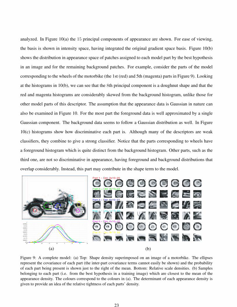
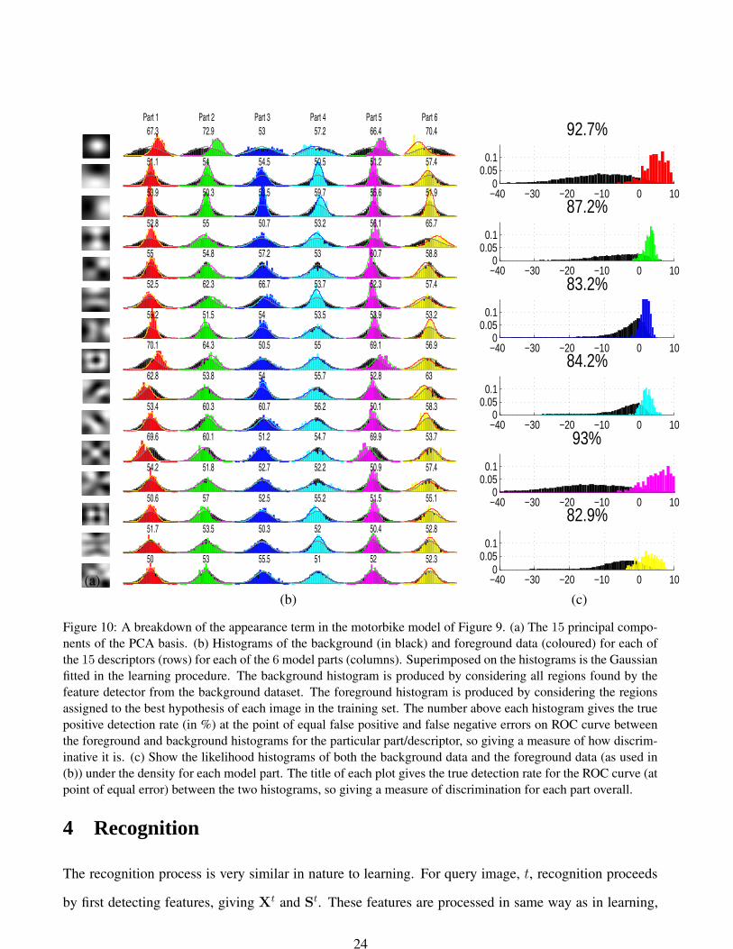
analyzed. In Figure 10(a) the 15 principal components of appearance are shown. For ease of viewing,

the basis is shown in intensity space, having integrated the original gradient space basis. Figure 10(b)

shows the distribution in appearance space of patches assigned to each model part by the best hypothesis

in an image and for the remaining background patches. For example, consider the parts of the model

corresponding to the wheels of the motorbike (the 1st (red) and 5th (magenta) parts in Figure 9). Looking

at the histograms in 10(b), we can see that the 8th principal component is a doughnut shape and that the

red and magenta histograms are considerably skewed from the background histogram, unlike those for

other model parts of this descriptor. The assumption that the appearance data is Gaussian in nature can

also be examined in Figure 10. For the most part the foreground data is well approximated by a single

Gaussian component. The background data seems to follow a Gaussian distribution as well. In Figure

10(c) histograms show how discriminative each part is. Although many of the descriptors are weak

classifiers, they combine to give a strong classifier. Notice that the parts corresponding to wheels have

a foreground histogram which is quite distinct from the background histogram. Other parts, such as the

third one, are not so discriminative in appearance, having foreground and background distributions that

overlap considerably. Instead, this part may contribute in the shape term to the model.

0.87

0.991

1

0.9

0.42

-4 -3 -2 -1 0 1 2 3 4

0.05

0.1

0.15

0.2

0.25

0.3

0.35

0.4

0.45

0

(a)

Part 1 − Det: 2x10−25

Part 2 − Det: 8x10−22

Part 3 − Det: 6x10−21

Part 4 − Det: 1x10−20

Part 5 − Det: 2x10−26

Part 6 − Det: 6x10−22

(b)

Figure 9: A complete model: (a) Top: Shape density superimposed on an image of a motorbike. The ellipsesrepresent the covariance of each part (the inter-part covariance terms cannot easily be shown) and the probabilityof each part being present is shown just to the right of the mean. Bottom: Relative scale densities. (b) Samplesbelonging to each part (i.e. from the best hypothesis in a training image) which are closest to the mean of theappearance density. The colours correspond to the colours in (a). The determinant of each appearance density isgiven to provide an idea of the relative tightness of each parts’ density.

23

(a)

Part 1

67.3

51.1

53.9

52.8

55

52.5

59.2

70.1

62.8

53.4

69.6

54.2

50.6

51.7

50

Part 2

72.9

54

50.3

55

54.8

62.3

51.5

64.3

53.8

60.3

60.1

51.8

57

53.5

53

Part 3

53

54.5

53.5

50.7

57.2

66.7

54

50.5

54

60.7

51.2

52.7

52.5

50.3

55.5

Part 4

57.2

50.5

59.7

53.2

53

53.7

53.5

55

55.7

56.2

54.7

52.2

55.2

52

51

Part 5

66.4

51.2

55.6

56.1

60.7

52.3

53.9

69.1

52.8

50.1

69.9

50.9

51.5

50.4

52

Part 6

70.4

57.4

51.9

65.7

58.8

57.4

53.2

56.9

63

58.3

53.7

57.4

55.1

52.8

52.3

(b)

−40 −30 −20 −10 0 100

0.050.1

92.7%

−40 −30 −20 −10 0 100

0.050.1

87.2%

−40 −30 −20 −10 0 100

0.050.1

83.2%

−40 −30 −20 −10 0 100

0.050.1

84.2%

−40 −30 −20 −10 0 100

0.050.1

93%

−40 −30 −20 −10 0 100

0.050.1

82.9%

(c)

Figure 10: A breakdown of the appearance term in the motorbike model of Figure 9. (a) The 15 principal compo-nents of the PCA basis. (b) Histograms of the background (in black) and foreground data (coloured) for each ofthe 15 descriptors (rows) for each of the 6 model parts (columns). Superimposed on the histograms is the Gaussianfitted in the learning procedure. The background histogram is produced by considering all regions found by thefeature detector from the background dataset. The foreground histogram is produced by considering the regionsassigned to the best hypothesis of each image in the training set. The number above each histogram gives the truepositive detection rate (in %) at the point of equal false positive and false negative errors on ROC curve betweenthe foreground and background histograms for the particular part/descriptor, so giving a measure of how discrim-inative it is. (c) Show the likelihood histograms of both the background data and the foreground data (as used in(b)) under the density for each model part. The title of each plot gives the true detection rate for the ROC curve (atpoint of equal error) between the two histograms, so giving a measure of discrimination for each part overall.

4 Recognition

The recognition process is very similar in nature to learning. For query image, t, recognition proceeds

by first detecting features, giving Xt and S

t. These features are processed in same way as in learning,

24

giving A.

Once Xt, At and S

t have been obtained we then compute the likelihood ratio using (1). To determine

if an object is in the image, we should, according to (2) sum over all hypotheses. However, in practice

the best results are obtained by just selecting the best one, since the background images typically contain

many low-scoring hypotheses, which if combined can give a false alarm. The likelihood ratio, assuming

we take the ratio of the priors in (1) to be 1, is the same as the ratio of posteriors, R. This is then

compared to a threshold to make the object present/absent decision. This threshold is determined from

the training set to give the desired balance between false positives and false negatives.

If we wish to localize the object within the image, the best hypothesis is found and a bounding box

around it formed at its location. We then sum over all hypotheses which are within this box. If the total

is greater than the threshold then an instance of the object is placed at the centroid of the box and all

features within the box are deleted. The next best hypothesis is then found and the process repeated until

the sum of hypotheses within the box falls below the threshold. This procedure allows the localization

of multiple object instances within the image.

The same efficient search methods described in section 3.4 are used in the recognition process to

find the single best hypothesis. However, recognition is faster as the covariances are tight (as compared

with the initial values in the learning process) so the vast majority of hypotheses may safely be ignored.

However the large N and P mean the process still takes around 2–3 seconds per image to perform the

search, in addition to the 10 seconds/image needed to extract the features.

5 Results

A variety of experiments are carried out on a number of different datasets, each one being a different cat-

egory. Since the model only handles a single viewpoint, the datasets consist of images that are flipped so

that all instances face in a similar direction, although there is still variability in location and scale within

the images. Additional experiments are performed which are of an investigative nature, to elucidate the

properties of our model and include baseline methods.

For each experiment, the dataset are split randomly into two separate sets of equal size. The model

is then trained on the first and tested on the second. In recognition, the models are tested in both classi-

25

Correct Correct INCORRECT Correct Correct

Correct Correct Correct Correct Correct


Correct Correct Correct INCORRECT INCORRECT

Correct INCORRECT Correct Correct Correct

(a)

Correct INCORRECT Correct Correct Correct

Correct Correct Correct Correct INCORRECT

Correct Correct INCORRECT Correct Correct

Correct Correct Correct INCORRECT Correct


(b)

Figure 11: (a) The motorbike model from Fig. 9 evaluating a set of query images. The pink dots are featuresfound on each image and the coloured circles indicate the features of the best hypothesis in the image. The size ofthe circles indicates the scale of feature. The outcome of the classification is marked above each image, incorrectclassifications being highlighted in red. (b) The model evaluating query images consisting of scenes around Caltech– the negative test set.

fication and localisation roles.

In classification, where the task is to determine the presence or abscene of the object within the

image, the performance is evaluated by plotting receiver-operating characteristic (ROC) curves. To ease

comparisons we use a single point on the curve to summarize its performance, namely the point of equal

error (i.e. p(True positive)=1-p(False positive)) when testing against one of two background datasets.

For example a figure of 9% means that 91% of the foreground images are correctly classified but 9% of

the background images were incorrectly classified (i.e. thought to be foreground). While the number of

foreground test images varied between experiments, depending on the number of images available for

each category, the foreground and background sets are always of equal size.

In localisation, where the task is to place a bounding box around the object within the image, the

performance is evaluated using recall-precision curves (RPC)2 , since the concept of a true negative is

less clear in this application. To be considered a correct detection, the area of overlap, ao between the

estimated bounding box B and the ground truth bounding box, Bgt must exceed 0.5 according to the2Recall is defined as the number of true positives over total positives in the data set, and precision is the number of true

positives over the sum of false positives and true positives.

26

criterion:

ao =area(B ∩ Bgt)

area(B ∪ Bgt)(19)

When evaluating the UIUC dataset, we adopt the same criterion as used in [2]. The experiments use

identical parameters for all categories. Images were scaled to 300 pixels in width, regions extracted at

scales between 10 and 30 pixels in radius. The gradient-based PCA with additional energy and residual

terms is used, with parameters: k = 21, l = 15. In learning, we use P = 6 and N = 20. N was increased

to 30 in recognition.

5.1 Datasets

Six diverse datasets were used in the experiments: motorbikes, airplanes, spotted cats, faces, cars (rear)

and cars (side). Examples from these datasets can be seen in Figure 1. The datasets of motorbikes,

airplanes, cars (rear), faces and cluttered scenes around Caltech (used as the negative test set) are avail-

able from our websites [11]. Two additional background datasets were used. The first is collected from

Google’s image search using the keyword “things”, resulting in a highly diverse collection of images.

The second is a set of empty road scenes for use as a realistic background test set for the cars (rear)

dataset. The cars (side) dataset is the UIUC dataset [1]. The spotted cat dataset, obtained from the Corel

database, is only 100 images originally, so another 100 were added by reflecting the original images,

making 200 in total. Amongst the datasets, only the motorbikes, airplanes and cars (rear) contained any

meaningful scale variation. All images from the datasets are converted to grayscale as colour is not used

in our experiments. Table 2 gives the size of training set used for each dataset in the experiments.

5.2 Experiments

Figures 12-14 show models and test images with a mix of correct and incorrect classifications for four

of the datasets. Notice how each model captures the essence, be it in appearance or shape or both, of the

object. The face and motorbike datasets have tight shape models, but some of the parts have a highly

variable appearance. For these parts any feature in that location will do regardless of what it looks like

(hence the probability of detection is 1). Conversely, the spotted cat dataset has a loose shape model,

but a highly distinctive appearance for each patch. In this instance, the model is just looking for patches

27

of spotty fur, regardless of their location. The differing nature of these examples illustrate the flexible

nature of the model.

The majority of errors are a result of the object receiving insufficient coverage from the feature detec-

tor. This happens for a number of reasons. One possibility is that, when a threshold is imposed on N (for

the sake of speed), many features on the object are removed. Alternatively, the feature detector seems to

perform badly when the object is much darker than the background (see examples in Figure 12). Finally,

the clustering of salient points into features, within the feature detector, is somewhat temperamental and

can result in parts of the object being missed. Table 3 shows a confusion table between the different

Dataset Total size of dataset (a) (b) (c)Motorbikes 800 3.3 3.3 6.0

Faces 435 10.6 8.3 10.1Airplanes 800 6.7 6.3 6.5

Spotted Cats 200 12.0 11.0 11.0Cars (Rear) 800 12.3 9.2 9.3

Table 2: Classification results on five datasets. (a) is the error rate(%) at the point of equal-error on an ROC curvefor a scale-variant model, testing against the Caltech background dataset (with the exception of Cars (rear) whichuses empty road scenes as the background test set). (b) is the same as (a) except that a scale-invariant model isused. (c) is the same as (b), except that the Google background dataset was used in testing.

categories, using the models evaluated in Table 2. Despite being inherently generative, the models can

distinguish between the categories well. The cars rear model seems to be somewhat weak, with many

car images being claimed by the airplane model.

Recognised categoryQuery image A C F S M

(A)irplane 88.8 6.0 0.3 0.7 4.2(C)ars (Rear) 19.7 67.0 0.8 3.3 9.2

(F)ace 2.8 1.4 86.2 2.3 7.3(S)potted Cats 3.0 1.0 3.0 76.0 17.0(M)otorbike 1.3 0.0 0.0 1.0 97.7

Table 3: Confusion table between the four categories. Each row gives a breakdown of how a query image of agiven category is classified (in %). No clutter dataset was used, rather images belonging to each category acted asnegative examples for models trained for the other categories. The optimum would be 100% on the diagonal withzero elsewhere.

Detection performance on the five datasets are shown in Figure 16. The predicted bounding box was

produced by taking the bounding box around the regions of the best hypothesis and then enlarging it by

28

0 0.5 1 1.5 2 2.5 3 3.5

−2

−1.5

−1

−0.5

0

0.5

1

1

1

1

1

1

Part 1 − Det: 8x10−28

Part 2 − Det: 6x10−29

Part 3 − Det: 6x10−26

Part 4 − Det: 3x10−28

Part 5 − Det: 6x10−28

Part 6 − Det: 7x10−27



Correct Correct Correct INCORRECT Correct

Correct INCORRECT Correct Correct


INCORRECT

Figure 12: A typical face model with 6 parts with a mix of correct and incorrect detections.

−0.5 0 0.5 1 1.5 2 2.5 3 3.5 4 4.5

−2

−1.5

−1

−0.5

0

0.5

1

1.5

2

11

1

11

1

Part 1 − Det: 2e−32






Correct INCORRECT Correct Correct

Correct

Correct Correct

Correct Correct

INCORRECT Correct Correct Correct

Correct Correct

INCORRECT

Figure 13: A typical spotted cat model with 6 parts. Note the loose shape model but distinctive “spotted fur”appearance.

29

0 1 2 3 4 5

−2

−1.5

−1

−0.5

0

0.5

1

1.5

2

2.5

1 1

11

1 1







CorrectINCORRECT

Correct CorrectCorrect

Correct

Correct

Correct Correct

INCORRECT Correct

Correct

Correct

Correct

Correct

INCORRECT

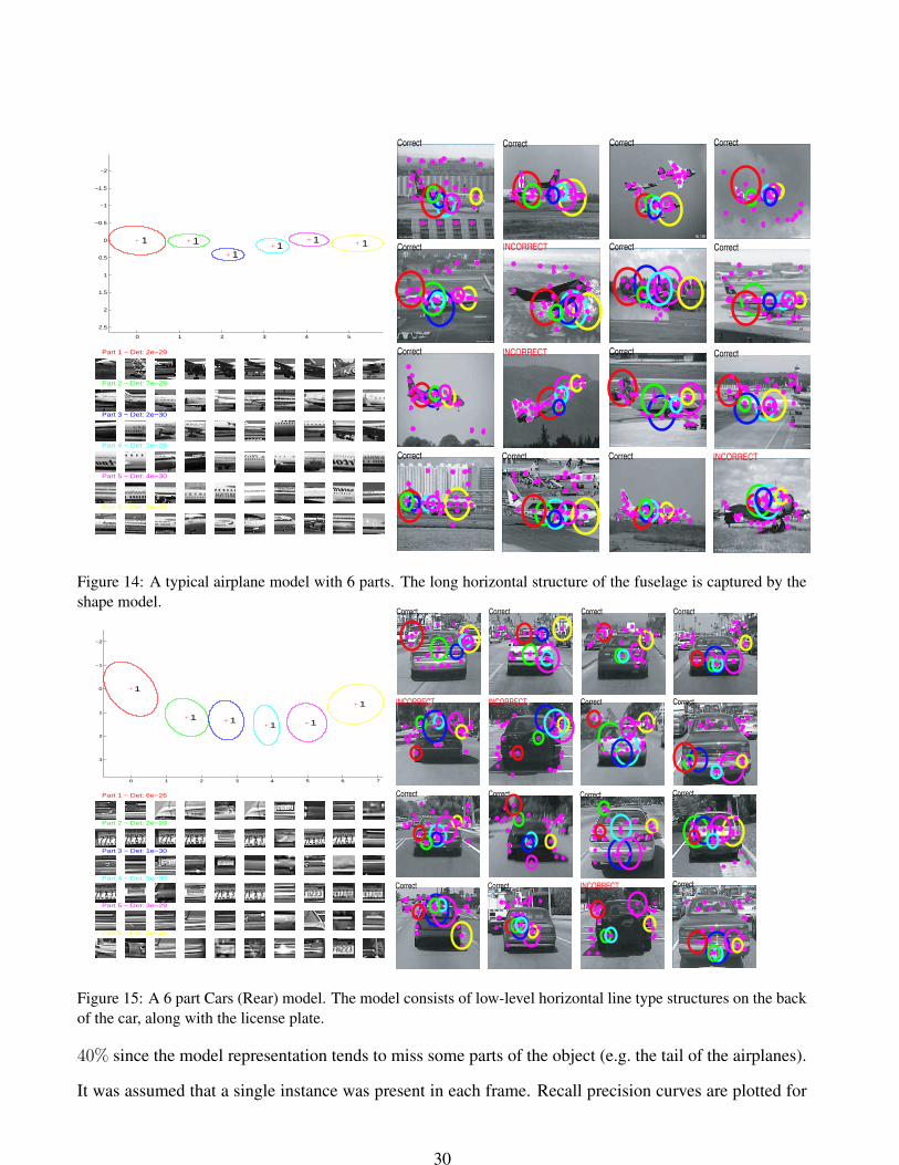
Figure 14: A typical airplane model with 6 parts. The long horizontal structure of the fuselage is captured by theshape model.

0 1 2 3 4 5 6 7

−2

−1

0

1

2

3

1

1 11 1

1







Correct

Correct

Correct Correct Correct Correct

INCORRECT INCORRECT Correct Correct

Correct Correct

Correct Correct

Correct

INCORRECT

Figure 15: A 6 part Cars (Rear) model. The model consists of low-level horizontal line type structures on the backof the car, along with the license plate.

40% since the model representation tends to miss some parts of the object (e.g. the tail of the airplanes).

It was assumed that a single instance was present in each frame. Recall precision curves are plotted for

30

0 0.1 0.2 0.3 0.4 0.5 0.6 0.7 0.8 0.9 10

0.1

0.2

0.3

0.4

0.5

0.6

0.7

0.8

0.9

1

Recall

Pre

scis

ion

Motorbikes

Scale invariant modelBaselineScale variant model

0 0.1 0.2 0.3 0.4 0.5 0.6 0.7 0.8 0.9 10

0.1

0.2

0.3

0.4

0.5

0.6

0.7

0.8

0.9

1

RecallP

rescis

ion

Airplanes


0 0.1 0.2 0.3 0.4 0.5 0.6 0.7 0.8 0.9 10

0.1

0.2

0.3

0.4

0.5

0.6

0.7

0.8

0.9

1

Recall

Pre

scis

ion

Faces


0 0.1 0.2 0.3 0.4 0.5 0.6 0.7 0.8 0.9 10

0.1

0.2

0.3

0.4

0.5

0.6

0.7

0.8

0.9

1

Recall

Pre

scis

ion

Cars Rear


0 0.1 0.2 0.3 0.4 0.5 0.6 0.7 0.8 0.9 10

0.1

0.2

0.3

0.4

0.5

0.6

0.7

0.8

0.9

1

Recall

Pre

scis

ion

Spotted Cats


PortionDataset inside box

Motorbikes 97.2Faces 57.9

Airplanes 78.9Spotted Cats 65.3Cars (Rear) 55.3

Figure 16: Recall-precision curves evaluating the localisation ability of the models for each of the five datasets.The fixed scale model is shown in blue; the scale-invariant model in red and a crude baseline in green. With theexception of cars rear, the fixed scale model preforms better than the scale-invariant one due to the lack of scalevariation in the data. The table lists the portion of regions lying within the ground truth bounding box of the objectfor each dataset. This is a crude measure for the difficulty of each category.

the fixed scale model; the scale-invariant model and a crude baseline, using the criterion in (19). The

baseline consists of assuming the object occupies the whole image and using the likelihood ratios for

each image from the scale-invariant model. Hence the baseline gives an indication of the total area the

objects occupy within the dataset. For example, the motorbikes tend to fill most of the frame so the

baseline beats two model variants. Another baseline measure is given in Figure 16(f) where we specify

the portion of regions inside the ground truth bounding box of the object. It is interesting to note that the

fixed-scale models beat the scale-invariant models since in many of the datasets the scale variation is not

that large and the scale-invariant model is making predictions within a larger space. The exception to this

is the cars (rear) dataset, where the scale variation is larger and the scale-invariant model outperforms

the scale variant one.

Using the cars (side) dataset, the ability of the model to perform multiple-instance localization is

tested. The training images were flipped to face in the same direction, but the test examples contained

31

cars of both orientations. Given the symmetry of the object, the right-facing model had little problem

picking out left-facing test examples. The model and test examples are shown in Figure 17, while the

recall precision curve comparing to Agarwal and Roth [2] is shown in Figure 25(a).

0 10 20 30 40 50 60 70

−30

−20

−10

0

10

20

0.94

0.74

0.9

0.860.89

0.7

0.91

Part 1 − Det: 4x10−12

Part 2 − Det: 1x10−12

Part 3 − Det: 6x10−12

Part 4 − Det: 9x10−12

Part 5 − Det: 1x10−11

Part 6 − Det: 5x10−13

Part 7 − Det: 4x10−12

Figure 17: The UIUC Cars (Side) dataset. The task here is to localize the object instance(s) within the image. Onthe left, we show the 7 part model. On the right, examples are shown from the test set, with correct localizationshighlighted in green, while false alarms are shown in red.

5.2.1 Baseline experiments

To put the performance of the model in context, we apply a variety of baseline methods to the datasets:

• Orientation histograms: The gradients of the whole image are computed and thresholded to remove

areas of very low gradient magnitude. An 8 bin histogram is computed of the orientations within

the gradient image, with weighting according to the magnitude of the gradient. Each image is thus

represented as by an 8-vector. The classifier consists of a single Gaussian density for both the

foreground and background class, modeling the mean and variance of the 8 histogram bins. The

parameters of these 8 dimensional densities are estimated from the training data. A query image

is evaluated by computing the likelihood ratio of the images’ 8-vector under the foreground and

background Gaussian models.

32

• Mean feature: The arithmetic mean of A in each image is computed, giving a 17-vector for each

image. The classifier consists of a single Gaussian density for both the foreground and background

class. The parameters of these 17 dimensional densities are estimated from the training data. A

query image is evaluated by computing the likelihood ratio of the images’ 17-vector under the

foreground and background Gaussian models. This baseline method is designed to reveal the

discriminative power of feature detector itself.

• PCA: Each image is resized to a 21x21 patch. After appropriate normalisation, it is then projected

into a 25 dimensional PCA basis (precomputed and the same for all categories). The classifier

consists of a single Gaussian density for both the foreground and background class, modeling the

coefficients of each basis vector. The parameters of these 25 dimensional densities are estimated

from the training data. A query image is evaluated by computing the likelihood ratio of the images’

25-vector under the foreground and background Gaussian models.

In Figures 18(a)-(e), we show ROC curves for the three baseline methods and the constellation model on

the five datasets in a classification task. The high performance of the baseline methods shows that the

datasets are not all that difficult. Nevertheless, the constellation model is only beaten in one case - cars

(rear) - by the PCA baseline. In Figure 18(f) we compare the performance in a multi-class setting by

giving the mean diagonal of a confusion table over the five categories for each of the approaches, with

the constellation model beating the baselines.

5.3 Analysis of performance

We look at the model working under various different conditions such as altering the number of model

parts; contaminating the training data, and removing terms from the model.

5.3.1 Changing scale of features

If the scale range of the saliency operator is changed, the set of regions extracted also changes, resulting

in a different model being learnt. Figure 19 shows the effects of altering the feature scale on the face

dataset. Figures 19(a) & (b) show a model using regions extracted using a hand selected scale range of

5-12 pixels in radius. The model picks out the eyes as well as the hairline. The standard scale range of

33

0 0.1 0.2 0.3 0.4 0.5 0.6 0.7 0.8 0.9 10

0.1

0.2

0.3

0.4

0.5

0.6

0.7

0.8

0.9

1

p(False Alarm)

p(D

ete

ction)

Motorbikes

Constellation modelPCAMean featureOrientation histogram

(a)

0 0.1 0.2 0.3 0.4 0.5 0.6 0.7 0.8 0.9 10

0.1

0.2

0.3

0.4

0.5

0.6

0.7

0.8

0.9

1

p(False Alarm)

p(D

ete

ction)

Airplanes


(b)

0 0.1 0.2 0.3 0.4 0.5 0.6 0.7 0.8 0.9 10

0.1

0.2

0.3

0.4

0.5

0.6

0.7

0.8

0.9

1

p(False Alarm)

p(D

ete

ction)

Cars Rear


(c)

0 0.1 0.2 0.3 0.4 0.5 0.6 0.7 0.8 0.9 10

0.1

0.2

0.3

0.4

0.5

0.6

0.7

0.8

0.9

1

p(False Alarm)

p(D

ete

ction)

Faces


(d)

0 0.1 0.2 0.3 0.4 0.5 0.6 0.7 0.8 0.9 10

0.1

0.2

0.3

0.4

0.5

0.6

0.7

0.8

0.9

1

p(False Alarm)

p(D

ete

ction)

Leopards


(e)

% on MeanApproach diagonal

Constellation model 83.1PCA 77.3

Mean feature 78.8Orientation histogram 58.8

Figure 18: ROC curves of the baseline experiments on the five datasets (a)–(e). The red curve is the constellationmodel while the green, blue and magenta curves are PCA; the mean feature and orientation histogram baselinesrespectively. The constellation model beats the baselines in all cases except for the cars rear dataset. (f) The tablegives the mean diagonal of a confusion table across all five datasets for the 4 different approaches.

10-30 pixels in radius results in a model shown in Figures 19(c) & (d). The eyes are no longer picked up

by the model, which relies entirely on the hairline. Both the models have similar error rates however of

8.3% for the generic scale setting and 10.1% for the hand-tuned one.

This illustrates that while the output of the feature detector varies depending on the settings used,

the ability of the learning algorithm to find consistency within whatever feature set it is given makes the

algorithm as a whole less sensitive to the performance of the feature detector.

5.3.2 Feature Representation

We now investigate different methods of representing the appearance of the regions within an image.

In Section 5.2 we used a 15 dimensional gradient-based PCA approach with two additional dimensions

34

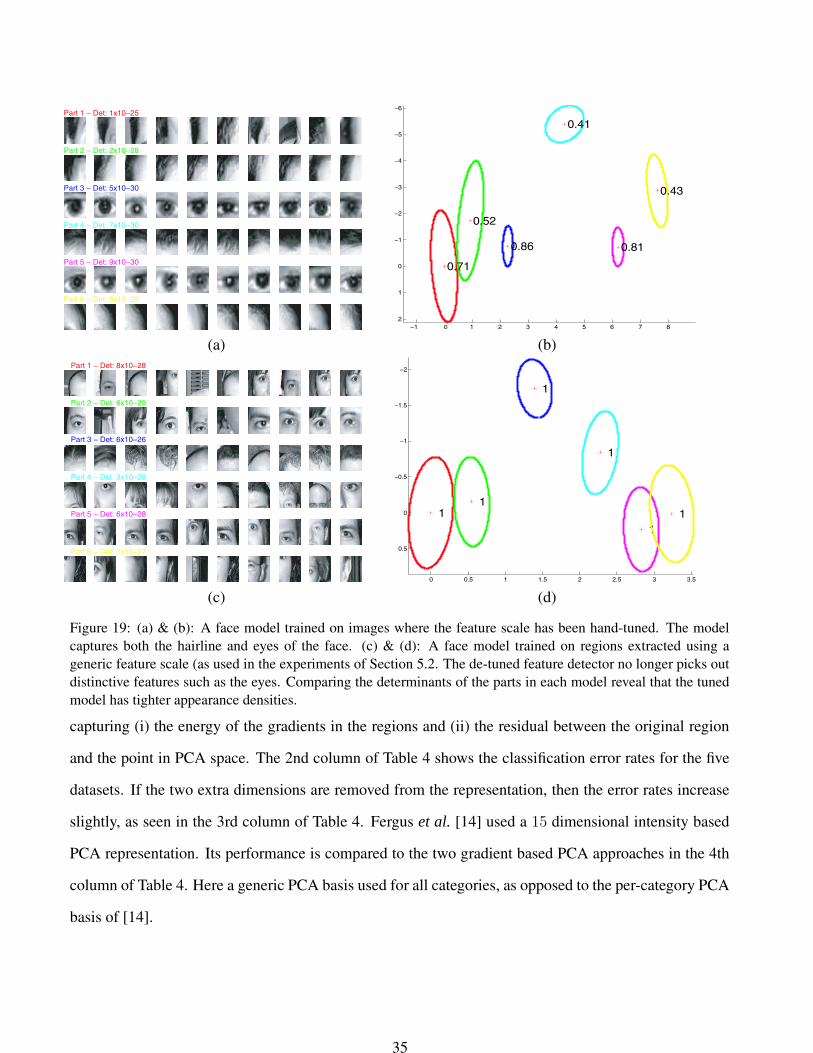
Part 1 − Det: 1x10−25

Part 2 − Det: 2x10−28

Part 3 − Det: 5x10−30

Part 4 − Det: 7x10−30

Part 5 − Det: 9x10−30

Part 6 − Det: 8x10−29

(a)−1 0 1 2 3 4 5 6 7 8

−6

−5

−4

−3

−2

−1

0

1

2

0.71

0.52

0.86

0.41

0.81

0.43

(b)Part 1 − Det: 8x10−28

Part 2 − Det: 6x10−29

Part 3 − Det: 6x10−26

Part 4 − Det: 3x10−28

Part 5 − Det: 6x10−28

Part 6 − Det: 7x10−27

(c)0 0.5 1 1.5 2 2.5 3 3.5

−2

−1.5

−1

−0.5

0

0.5

1

1

1

1

1

1

(d)

Figure 19: (a) & (b): A face model trained on images where the feature scale has been hand-tuned. The modelcaptures both the hairline and eyes of the face. (c) & (d): A face model trained on regions extracted using ageneric feature scale (as used in the experiments of Section 5.2. The de-tuned feature detector no longer picks outdistinctive features such as the eyes. Comparing the determinants of the parts in each model reveal that the tunedmodel has tighter appearance densities.

capturing (i) the energy of the gradients in the regions and (ii) the residual between the original region

and the point in PCA space. The 2nd column of Table 4 shows the classification error rates for the five

datasets. If the two extra dimensions are removed from the representation, then the error rates increase

slightly, as seen in the 3rd column of Table 4. Fergus et al. [14] used a 15 dimensional intensity based

PCA representation. Its performance is compared to the two gradient based PCA approaches in the 4th

column of Table 4. Here a generic PCA basis used for all categories, as opposed to the per-category PCA

basis of [14].

35

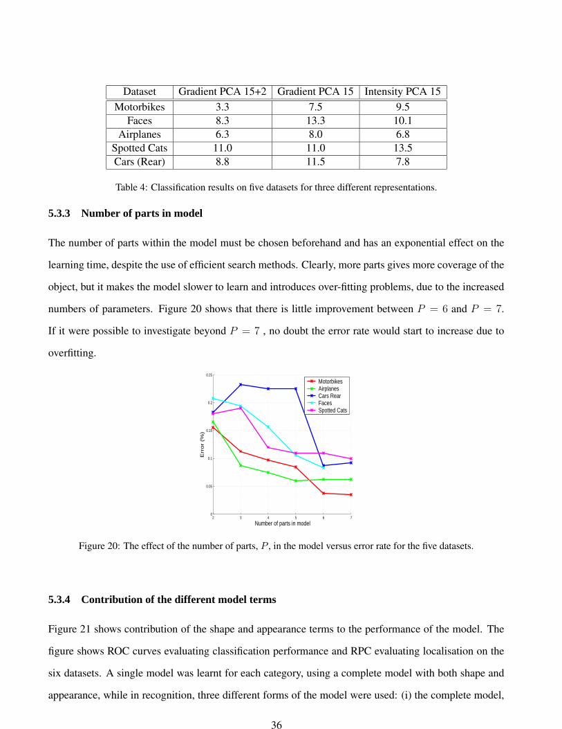
Dataset Gradient PCA 15+2 Gradient PCA 15 Intensity PCA 15Motorbikes 3.3 7.5 9.5

Faces 8.3 13.3 10.1Airplanes 6.3 8.0 6.8

Spotted Cats 11.0 11.0 13.5Cars (Rear) 8.8 11.5 7.8

Table 4: Classification results on five datasets for three different representations.

5.3.3 Number of parts in model

The number of parts within the model must be chosen beforehand and has an exponential effect on the

learning time, despite the use of efficient search methods. Clearly, more parts gives more coverage of the

object, but it makes the model slower to learn and introduces over-fitting problems, due to the increased

numbers of parameters. Figure 20 shows that there is little improvement between P = 6 and P = 7.

If it were possible to investigate beyond P = 7 , no doubt the error rate would start to increase due to

overfitting.

2 3 4 5 6 70

0.05

0.1

0.15

0.2

0.25

Number of parts in model

Err

or

(%)

MotorbikesAirplanesCars RearFacesSpotted Cats

Figure 20: The effect of the number of parts, P , in the model versus error rate for the five datasets.

5.3.4 Contribution of the different model terms

Figure 21 shows contribution of the shape and appearance terms to the performance of the model. The

figure shows ROC curves evaluating classification performance and RPC evaluating localisation on the

six datasets. A single model was learnt for each category, using a complete model with both shape and

appearance, while in recognition, three different forms of the model were used: (i) the complete model,

36

(ii) the complete model, but ignoring the appearance term and (iii) the complete model, but ignoring the

shape term. Across all six datasets, it is noticeable that the appearance term appears to be more important

than the shape for classification. Only in the case of airplanes did the shape-only model perform well.

Indeed, for cars (rear) the removal of the shape term actually improves the performance slightly. This

is due to the ordering constraint imposed on the shape which in this case may be removing the best

hypothesis from each frame. However, when the task is localisation, the shape-only model outperforms

the appearance only one. In some cases the difference is dramatic, e.g. airplanes and cars (side).

When learning was performed with degraded models, the use of the appearance component alone

produced a model with a performance close to that of the full model. However, when using only the

shape component, the models frequently did not converge to a meaningful model, resulting in chance

level classification performance.

5.3.5 Over-fitting

The large number of parameters in the model, as shown in table 1, means that a large number of images

are needed in training to avoid over-fitting the training data. Figure 22 shows that around 250 images are

needed in training for the model to generalize well. Surprisingly, a relatively small number of training

examples is sufficient for the in-sample error and out-of-sample error curves to converge. The use of

priors in learning can dramatically reduce the training requirement on the number of images, down to

just a handful or even one. See Fei-Fei et al. [9] for a Bayesian extension to the constellation model,

incorporating such priors in learning.

5.3.6 Contamination of the training set

Collecting hundreds of images of a given category of sufficient quality is a laborious time-consuming job.

Being able to learn from datasets where some of the images consist only of clutter or are of insufficient

quality is a useful property since it simplifies the task of building a training set. In Figure 23 we show the

results of deliberately introducing background images into a training set. It is pleasing to note that for

most of the datasets, the drop in performance is small even with 50% background images in the training

set. The model handles this level of contamination by interpreting the background images as ones where

all the model parts are occluded. Notice that the graph bottoms out at around 20%–30% correct when

37

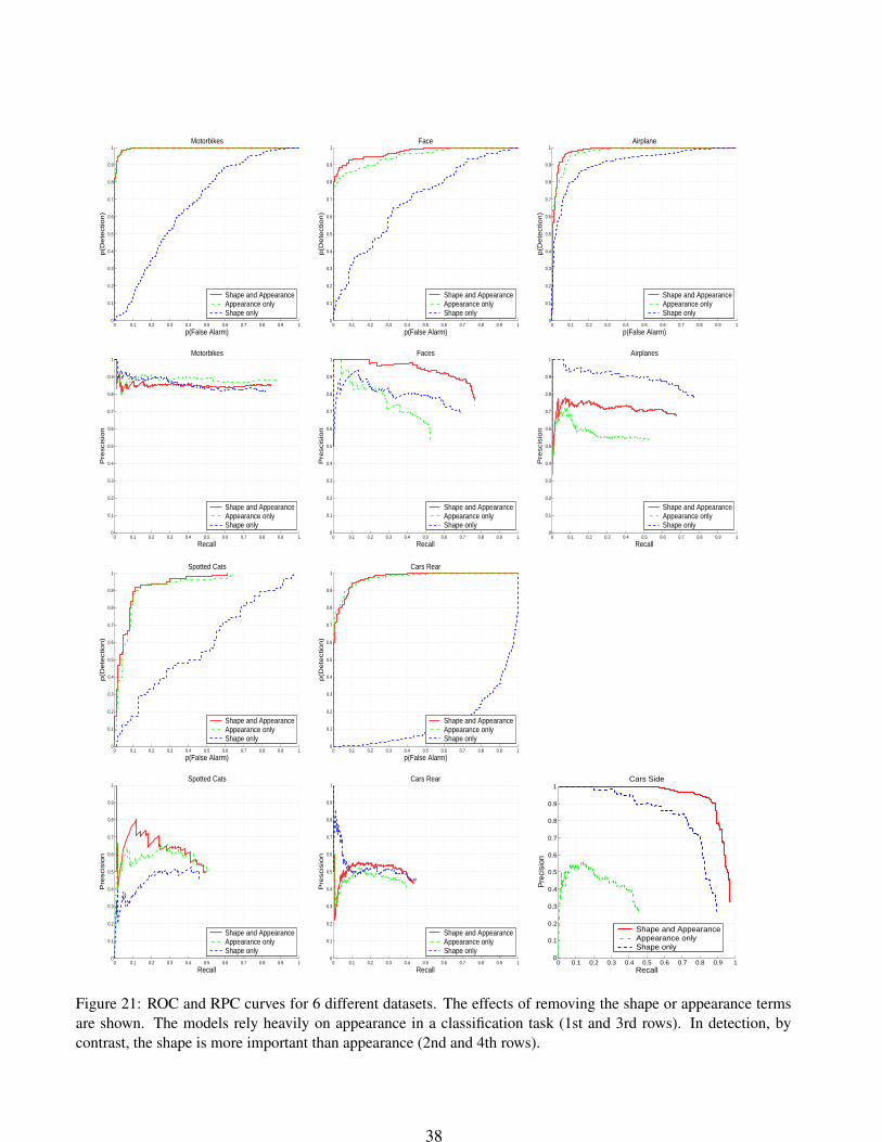
0 0.1 0.2 0.3 0.4 0.5 0.6 0.7 0.8 0.9 10

0.1

0.2

0.3

0.4

0.5

0.6

0.7

0.8

0.9

1

p(D

ete

ctio

n)

p(False Alarm)

Motorbikes

Shape and AppearanceAppearance onlyShape only

0 0.1 0.2 0.3 0.4 0.5 0.6 0.7 0.8 0.9 10

0.1

0.2

0.3

0.4

0.5

0.6

0.7

0.8

0.9

1

p(D

ete

ctio

n)

p(False Alarm)

Face


0 0.1 0.2 0.3 0.4 0.5 0.6 0.7 0.8 0.9 10

0.1

0.2

0.3

0.4

0.5

0.6

0.7

0.8

0.9

1

p(D

ete

ctio

n)

p(False Alarm)

Airplane


0 0.1 0.2 0.3 0.4 0.5 0.6 0.7 0.8 0.9 10

0.1

0.2

0.3

0.4

0.5

0.6

0.7

0.8

0.9

1

Recall

Pre

scis

ion

Motorbikes


0 0.1 0.2 0.3 0.4 0.5 0.6 0.7 0.8 0.9 10

0.1

0.2

0.3

0.4

0.5

0.6

0.7

0.8

0.9

1

Recall

Pre

scis

ion

Faces


0 0.1 0.2 0.3 0.4 0.5 0.6 0.7 0.8 0.9 10

0.1

0.2

0.3

0.4

0.5

0.6

0.7

0.8

0.9

1

RecallP

rescis

ion

Airplanes


0 0.1 0.2 0.3 0.4 0.5 0.6 0.7 0.8 0.9 10

0.1

0.2

0.3

0.4

0.5

0.6

0.7

0.8

0.9

1

p(D

ete

ctio

n)

p(False Alarm)

Spotted Cats


0 0.1 0.2 0.3 0.4 0.5 0.6 0.7 0.8 0.9 10

0.1

0.2

0.3

0.4

0.5

0.6

0.7

0.8

0.9

1

p(D

ete

ctio

n)

p(False Alarm)

Cars Rear


0 0.1 0.2 0.3 0.4 0.5 0.6 0.7 0.8 0.9 10

0.1

0.2

0.3

0.4

0.5

0.6

0.7

0.8

0.9

1

Recall

Pre

scis

ion

Spotted Cats


0 0.1 0.2 0.3 0.4 0.5 0.6 0.7 0.8 0.9 10

0.1

0.2

0.3

0.4

0.5

0.6

0.7

0.8

0.9

1

Recall

Pre

scis

ion

Cars Rear


0 0.1 0.2 0.3 0.4 0.5 0.6 0.7 0.8 0.9 10

0.1

0.2

0.3

0.4

0.5

0.6

0.7

0.8

0.9

1

Pre

cisi

on

Recall

Cars Side


Figure 21: ROC and RPC curves for 6 different datasets. The effects of removing the shape or appearance termsare shown. The models rely heavily on appearance in a classification task (1st and 3rd rows). In detection, bycontrast, the shape is more important than appearance (2nd and 4th rows).

38

0 1 2 3 4 5 6 7 8 90

5

10

15

20

25

30

35

40

45

50

log2 (# training images)

RO

C E

qual E

rror

Rate

(%

)

3 parts

(a)

0 1 2 3 4 5 6 7 8 90

5

10

15

20

25

30

35

40

45

50


RO

C E

qual E

rror

Rate

(%

)

4 parts

(b)

0 1 2 3 4 5 6 7 8 90

5

10

15

20

25

30

35

40

45

50


RO

C E

qual E

rror

Rate

(%

)

5 parts

(c)

0 1 2 3 4 5 6 7 8 90

5

10

15

20

25

30

35

40

45

50


RO

C E

qual E

rror

Rate

(%

)

6 parts

(d)

Figure 22: (a)-(d) The training (red) and test (blue dot-dashed) errors versus the number of training images for themotorbike dataset with models having (a) 3 parts, (b) 4 parts, (c) 5 parts, (d) 6 parts. Note the log scale on thex-axis. The curves converge to the Bayes’ error once the number of training images is 256. The error bars showtwo standard deviations on performance, computed from 10 runs for 2–64 training images and 5 runs for 128–400images.

the training set is entirely background images, while one would have expected 50% correct. This implies

that the background images contain some structure that is being learnt by the model, implying that our

assumptions about the nature of the background are not strictly true. In [12], the problem of learning

from contaminated data is investigated in more depth.

5.3.7 Sampling from the model

Since our models are generative in nature we can sample from them. However, we are not able to di-

rectly sample back into pixel-space since the use of PCA for appearance introduces a non-probabilistic

39

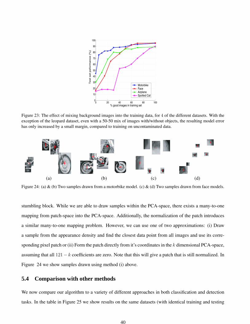
0 20 40 60 80 1000

10

20

30

40

50

60

70

80

90

100

% good images in training set

Test se

t pefo

rma

nce (

%)

MotorbikeFaceAirplaneSpotted Cat

Figure 23: The effect of mixing background images into the training data, for 4 of the different datasets. With theexception of the leopard dataset, even with a 50-50 mix of images with/without objects, the resulting model errorhas only increased by a small margin, compared to training on uncontaminated data.

(a) (b) (c) (d)Figure 24: (a) & (b) Two samples drawn from a motorbike model. (c) & (d) Two samples drawn from face models.

stumbling block. While we are able to draw samples within the PCA-space, there exists a many-to-one

mapping from patch-space into the PCA-space. Additionally, the normalization of the patch introduces

a similar many-to-one mapping problem. However, we can use one of two approximations: (i) Draw

a sample from the appearance density and find the closest data point from all images and use its corre-

sponding pixel patch or (ii) Form the patch directly from it’s coordinates in the k dimensional PCA-space,

assuming that all 121− k coefficients are zero. Note that this will give a patch that is still normalized. In

Figure 24 we show samples drawn using method (i) above.

5.4 Comparison with other methods

We now compare our algorithm to a variety of different approaches in both classification and detection

tasks. In the table in Figure 25 we show results on the same datasets (with identical training and testing

40

images) for the following algorithms: an earlier incarnation of the constellation model by Weber et al.

[43, 40]; the region-based discriminative SVM-based method of Opelt et al. [31]; the bag-of-words pLSA

approach of Sivic et al. [35] and the Hough space voting scheme of Leibe et al. [25]. The table also lists

the supervision required in training. The performance of the model can be seen to be comparable to the

other approaches, beating the other methods in the majority of cases. Although the method of Leibe et al.

[25] achieves better performance, it requires the manual segmentation of the objects within the training

images and has only been applied to a subset of the categories.

Figure 25 shows a recall-precision curve comparing the algorithm to Agarwal and Roth [2], with our

algorithm showing a distinct improvement. The superior performance of Leibe et al. [25] on this dataset

may be explained by the use of a validation scheme in their approach, which helps to eliminate false

positives.

Method Ours Weber [43, 40] Opelt [31] Sivic [35] Leibe [25]Supervision I I I N I,SMotorbikes 3.3 16.0 7.8 15.4 6.0

Faces 8.3 6.0 6.5 5.3 -Airplanes 6.3 32.0 11.1 3.4 -

Spotted Cats 11.0 - - - -Cars Rear 8.8 - 8.9 21.4 6.1Cars Side 11.5 - 17.0 - 3.0

Figure 25: Comparison to other methods [2, 25, 31, 35, 40, 43]. The diagram on the left shows the RPC for [2] andour algorithm on the cars (side) dataset. On the right the table gives ROC equal error rates (except for the car (side)dataset where it is a recall-precision equal error) on a number of datasets. The second row shows the supervisionrequired in training for each method: N - None; I - Image labels and flipping to give consistent viewpoint; S -Object segmentation.

6 Conclusions and Further work

We have proposed an improved learning scheme for the ‘constellation model’ which is scale-invariant

and where shape and appearance are learnt simultaneously. We tested an implementation of such a

scheme on six diverse datasets. We find that learning is robust with respect to clutter, scale variation and

inter-object variability. Given exemplars of a similar pose, no futher human intervention is required to

segment, normalize or otherwise preprocess the training data.

We have compared directly to the previous work on the constellation model of Weber et al. and shown

41

an improvement in performance (see Figure 25). We feel that the key improvement is that appearance

and shape are learnt simultaneously, giving a cleaner learning scheme that avoids the reliance of first

obtaining a good appearance model before the shape can be learnt. In the scheme of Weber et al. , the

clustering procedure to form a codebook of possibly useful features is a vital step. Examination of cases

where the approach fails reveals that the codebook consists of a large number of generic features such as

orientated edges which are not discriminative.

We have also compared to a wide variety of other approaches and baseline methods and shown the

our approach compares favorably with them. The baseline methods reveal the limitations of our datasets

and therefore harder datasets should be adopted.

We find that when our algorithm fails to detect the presence of an object, the most frequent cause

of this false-reject error is that an insufficient number of features were detected by the front-end feature

finder. It is clear that better feature finders as well as a more diverse array of features (e.g. sections of

contours) should be employed.

Other observations: (a) the system works well both on artificial (cars, planes, motorcycles) and nat-

ural (faces,cats) data; (b) while this paper uses many categories, it is clear that now we need to push

forward with experiments involving hundreds of categories; (c) colour was not exploited and for some

categories this may be important; (d) for classification, the appearance of parts seems more useful than

their relative location, therefore some simplification of the shape term might reduce the computational

complexity of both learning and recognition, as well as reducing the number of parameters in the model

(see [6, 13] for an investigation of this point); (e) we have made a number of design choices (size of

patches, Gaussian distributions, parameterizations etc. ) which were guided by common sense and need

to be validated experimentally; (f) we find that our method is parsimonious in the number of training ex-

amples that are needed to train a model of a given complexity. However, it would be clearly advantageous

to further reduce this number [9].

A serious drawback of the current approach is that it is limited to a single viewpoint. Extensions

to multiple views would be an important addition to the model. One approach is to use a mixture of

constellation models in the manner of Weber et al. [41], each mixture component handling a separate

view.

42

There are two other areas where improvements will be very beneficial. The first is in a further

generalization of the model structure to have a multi-modal appearance density with a single shape

distribution. This will allow more complex appearances to be represented, for example faces with and

without sunglasses. Second, we have built in scale-invariance, but greater invariance should also be

possible. This would enable learning and recognition from images with much larger viewpoint variation.

For example, similarity invariance can be achieved in recognition by searching over rotations.

Acknowledgments

Timor Kadir for advice on the feature detector. D. Roth for providing the Cars (Side) dataset. Funding

was provided by National Science Foundation Engineering Research Center for Neuromorphic Systems

Engineering, the UK EPSRC, EC Project CogViSys and PASCAL Network of Excellence.

References

[1] S. Agarwal, A. Awan, and D. Roth. Uiuc car dataset. http://l2r.cs.uiuc.edu/ cogcomp/Data/Car/,

2002.

[2] S. Agarwal and D. Roth. Learning a sparse representation for object detection. In Proceedings of

the European Conference on Computer Vision, pages 113–130, 2002.

[3] Y. Amit and D. Geman. A computational model for visual selection. Neural Computation,

11(7):1691–1715, 1999.

[4] E. Borenstein. and S. Ullman. Class-specific, top-down segmentation. In Proceedings of the Euro-

pean Conference on Computer Vision, pages 109–124, 2002.

[5] M. Burl, M. Weber, and P. Perona. A probabilistic approach to object recognition using local

photometry and global geometry. In Proceedings of the European Conference on Computer Vision,

pages 628–641, 1998.

43

[6] D. Crandall, P. Felzenszwalb, and D. Huttenlocher. Spatial priors for part-based recognition us-

ing statistical models. In Proceedings of the IEEE Conference on Computer Vision and Pattern

Recognition, San Diego, volume 1, pages 10–17, 2005.

[7] G. Csurka, C. Bray, C. Dance, and L. Fan. Visual categorization with bags of keypoints. In

Workshop on Statistical Learning in Computer Vision, ECCV, pages 1–22, 2004.

[8] A. Dempster, N. Laird, and D. Rubin. Maximum likelihood from incomplete data via the EM

algorithm. JRSS B, 39:1–38, 1976.

[9] L. Fei-Fei, R. Fergus, and P. Perona. A Bayesian approach to unsupervised one-shot learning of

object categories. In Proceedings of the 9th International Conference on Computer Vision, Nice,

France, pages 1134–1141, October 2003.

[10] P. Felzenszwalb and D. Huttenlocher. Pictorial structures for object recognition. In Proceedings of

the IEEE Conference on Computer Vision and Pattern Recognition, pages 2066–2073, 2000.

[11] R. Fergus and P. Perona. Caltech object category datasets. http://www.vision.caltech.edu/html-

files/archive.html, 2003.

[12] R. Fergus, P. Perona, and A. Zisserman. A visual category filter for google images. In Proceedings

of the 8th European Conference on Computer Vision, Prague, Czech Republic, pages 242–256.

Springer-Verlag, May 2004.

[13] R. Fergus, P. Perona, and A. Zisserman. A sparse object category model for efficient learning and

exhaustive recognition. In Proceedings of the IEEE Conference on Computer Vision and Pattern

Recognition, San Diego, volume 1, pages 380–387, 2005.

[14] R. Fergus, P. Perona, and P. Zisserman. Object class recognition by unsupervised scale-invariant

learning. In Proceedings of the IEEE Conference on Computer Vision and Pattern Recognition,

2003.

[15] R. Fergus, M. Weber, and P. Perona. Efficient methods for object recognition using the constellation

model. Technical report, California Institute of Technology, 2001.

44

[16] D. A. Forsyth and J. Ponce. Computer Vision: A modern approach. Prentice Hall, 2002.

[17] W. E. L. Grimson and T. Lozano-Perez. Localizing overlapping parts by searching the interpretation

tree. IEEE Transactions on Pattern Analysis and Machine Intelligence, 9(4):469–482, 1987.

[18] P. Hart, N. Nilsson, and B. Raphael. A formal basis for the determination of minimum cost paths.

IEEE Transactions on SSC, 4:100–107, 1968.

[19] B. Heisele, T. Serre, M. Pontil, T. Vetter, and T. Poggio. Categorization by learning and combin-

ing object parts. In Advances in Neural Information Processing Systems 14, Vancouver, Canada,

volume 2, pages 1239–1245, 2002.

[20] M. Jerrum and A. Sinclair. The Markov chain Monte Carlo method. In D. S. Hochbaum, editor,

Approximation Algorithms for NP-hard Problems. PWS Publishing, Boston, 1997.

[21] F. Jurie and C. Schmid. Scale-invariant shape features for recognition of object categories. In

Proceedings of the IEEE Conference on Computer Vision and Pattern Recognition, Washington,

DC, pages 90–96, 2004.

[22] T. Kadir and M. Brady. Scale, saliency and image description. International Journal of Computer

Vision, 45(2):83–105, 2001.

[23] Y. Ke and R. Sukthankar. PCA-SIFT: A more distinctive representation for local image descriptors.

In Proceedings of the IEEE Conference on Computer Vision and Pattern Recognition, Washington,

DC, June 2004.

[24] Y. LeCun, F. Huang, and L. Bottou. Learning methods for generic object recognition with invari-

ance to pose and lighting. In Proceedings of the IEEE Conference on Computer Vision and Pattern

Recognition, Washington, DC. IEEE Press, 2004.

[25] B. Leibe, A. Leonardis, and B. Schiele. Combined object categorization and segmentation with an

implicit shape model. In Workshop on Statistical Learning in Computer Vision, ECCV, 2004.

[26] T. Leung, M. Burl, and P. Perona. Probabilistic affine invariants for recognition. In Proceedings of

the IEEE Conference on Computer Vision and Pattern Recognition, pages 678–684, 1998.

45

[27] T. Lindeberg. Feature detection with automatic scale selection. International Journal of Computer

Vision, 30(2):77–116, 1998.

[28] D. G. Lowe. Perceptual Organization and Visual Recognition. Kluwer Academic Publishers, 1985.

[29] K.V. Mardia and I.L. Dryden. “Shape Distributions for Landmark Data”. Adv. Appl. Prob., 21:742–

755, 1989.

[30] K. Mikolajczyk and C. Schmid. Indexing based on scale invariant interest points. In Proceedings of

the 8th International Conference on Computer Vision, Vancouver, Canada, pages 525–531, 2001.

[31] A. Opelt, A. Fussenegger, and P. Auer. Weak hypotheses and boosting for generic object detection

and recognition. In Proceedings of the 8th European Conference on Computer Vision, Prague,

Czech Republic, 2004.

[32] H. Rowley, S. Baluja, and T. Kanade. Neural network-based face detection. IEEE Transactions on

Pattern Analysis and Machine Intelligence, 20(1):23–38, Jan 1998.

[33] C. Schmid. Constructing models for content-based image retrieval. In Proceedings of the IEEE

Conference on Computer Vision and Pattern Recognition, volume 2, pages 39–45, 2001.

[34] H. Schneiderman and T. Kanade. A statistical approach to 3D object detection applied to faces and

cars. In Proc. Computer Vision and Pattern Recognition, pages 746–751, 2000.

[35] J. Sivic, B. Russell, A. Efros, A. Zisserman, and W. Freeman. Discovering object categories in

image collections. Technical Report A. I. Memo 2005-005, Massachusetts Institute of Technology,

2005.

[36] K. Sung and T. Poggio. Example-based learning for view-based human face detection. IEEE

Transactions on Pattern Analysis and Machine Intelligence, 20(1):39–51, Jan 1998.

[37] J. Thureson and S. Carlsson. Appearance based qualitative image description for object class recog-

nition. In Proceedings of the 8th European Conference on Computer Vision, Prague, Czech Repub-

lic, pages 518–529, 2004.

46

[38] A. Torralba, K. P. Murphy, and W. T. Freeman. Sharing features: efficient boosting procedures

for multiclass object detection. In Proceedings of the IEEE Conference on Computer Vision and

Pattern Recognition, Washington, DC, pages 762–769, 2004.

[39] P. Viola and M. Jones. Rapid object detection using a boosted cascade of simple features. In

Proceedings of the IEEE Conference on Computer Vision and Pattern Recognition, pages 511–518,

2001.

[40] M. Weber. Unsupervised Learning of Models for Object Recognition. PhD thesis, California

Institute of Technology, Pasadena, CA, 2000.

[41] M. Weber, W. Einhauser, M. Welling, and P. Perona. Viewpoint-invariant learning and detection

of human heads. In Proc. 4th IEEE Int. Conf. Autom. Face and Gesture Recog., FG2000, pages

20–27, March 2000.

[42] M. Weber, M. Welling, and P. Perona. Towards automatic discovery of object categories. In

Proceedings of the IEEE Conference on Computer Vision and Pattern Recognition, pages 101–109,

June 2000.

[43] M. Weber, M. Welling, and P. Perona. Unsupervised learning of models for recognition. In Pro-

ceedings of the European Conference on Computer Vision, pages 18–32, 2000.

47

weakly supervised scale-invariant learning of …fergus/papers/fergus_ijcv.pdfweakly supervised...

Documents