Weak and Strong Forms of Purchasing Power Parity

in the Long-Run

by Svetoslav Ivanov and Mischka Moechtar

May 2012

Introduction: This project is to test purchasing power parity of the US dollar against other foreign currencies. We performed a variety of tests using time-series regression: Augmented Dickey Fuller for stationarity, Engle Granger for cointegration, and vector error correction to find the number of cointegrating vectors between the time series using the Johansen test. We tested the purchasing power parity for the exchange rate between the US dollar and the Japanese yen, the British pound and the Canadian dollar from 1976 to 2012.

Theory: An exchange rate is the rate at which one currency can be exchanged for another. Exchange rates are determined in the foreign exchange market. Thus, economists predict that movements in exchange rates should reflect changes in the relative demand for and supply of the two currencies. Assuming supplies unchanged, if demand for US dollar goes up in relation to euro, the value of the dollar should rise: more euros should be exchanged for each dollar than before. In this case the US dollar appreciated, while the euro depreciated. Exchange rates are used to buy something in a market where the local currency is used as the conventional medium of exchange. This line of reasoning suggests that the international demand for a particular currency might depend on the underlying demand for the goods, services, and assets sold in markets using that currency. Because the currency of a particular country is most often used in markets where that country’s products are sold, the demand for the goods, services, and assets produced by a country might be a good proxy for the demand for its currency, i.e. we will observe the relationship between price levels of two different countries with respect to their exchange rates.

The theory of purchasing power parity is based on the notion that the exchange rate depends on relative price levels. Purchasing power parity states that the nominal exchange rate between two currencies should be equal to the ratio of aggregate price levels between the two countries, so that a unit of currency of one currency will have the same purchasing power in a foreign country. The mathematical expression we use to derive purchasing power parity implies that PUS = EPf, or E = PUS/pf, where E is the exchange rate in dollars per foreign currency, PUS is the dollar price of a basket of goods, and Pf is the foreign price for a basket of goods. This brings us to the concept of the law of one price, where we assume the goods and services of two different countries are sold with the same purchasing power. Therefore the exchange rate can be linked to the different price levels of two countries. If PPP holds then the price of an internationally traded good should be the same anywhere in the world once that price is expressed in a common currency since people could make a riskless profit by shipping the goods from locations where the price is low to locations where the price is high. There is only one exchange rate between any pair of currencies, and if PPP holds broadly, that same exchange rate must balance the relative prices of all the commodities. Thus, when PPP is considered as a theory of the exchange rate a very broad market basket of commodities must be used rather than just one commodity. Most testing of PPP is done with price indexes rather than with the price of individual goods and services. The general idea is that a unit of currency should be able to buy the same basket of goods in one country as the equivalent amount of foreign currency, at the going exchange rate can buy in a foreign country, so that there is parity in the purchasing power of the unit of currency across two economies.

We transformed our variables exchange rate with respect to the United States and the consumer price index level to logs. The exchange rates are expressed as the amount of foreign currency needed to exchange for each US$1. We will be testing long-run PPP employing bivariate tests, such as the ADF (augmented Dickey-Fuller) and Johansen’s maximum likelihood methods. A price index tells how much a particular market basket costs now relative to how much it cost in a chosen base year (= 2005). The market basket typically varies considerably across countries; each country chooses a basket that represents the composition of its output or consumption. In addition, there is no information about the absolute level of prices in the country, merely about how prices have changed since the base year. For this reason, we cannot compare CPI values of the United States with that of the UK. Because of this indeterminacy in absolute level of prices, a normalization constant was added to

the PPP relationship, such that: 𝐸𝑡 = 𝜆 𝑃𝑈𝑆

𝑃𝑓 In logarithmic terms, this leads to the

following equation:

ln𝐸𝑡 = 𝛼 + 𝛽(𝑙𝑛𝑃𝑡𝑈𝑆 − 𝑙𝑛𝑃𝑡𝑓),

All the equations are written with the exchange rate as the dependent variable and the two countries’ price level difference as independent variables. We assume the shocks to the exchange rate must not affect inflation rate in either country. Under pure floating rates, the central bank commits itself to a monetary policy based solely on internal considerations such as its desired inflation rate and the exchange rate adapts itself to maintain PPP. In our study, all four countries have floating exchange rate. Otherwise, if the exchange rate is pegged, the money supply of a particular country will be endogenously driven to establish the inflation rate at a level consistent with the US$ inflation and the desired rate of change of the exchange rate. In order to test PPP, we chose a time interval of a month from 1976 to 2012 and chose to use consumer price index. We prefer to use larger range for the dataset because it is likely there are delays in the response of exchange rates to price differentials. The high frequency nature of our data yields more data points thus we can assume most asymptotic properties of the distributions. The most common price indexes are the consumer price index (CPI), the producer price index (PPI), and the price deflator for GDP (PGDP). CPI focuses on a market basket that is typical of the purchases of urban consumers. The PPI is an index of the prices of industrial goods often bought by large industrial firms. The PGDP covers all goods and services produced in the economy. We chose the CPI because it is more representative of the entire economy’s prices, despite being composed of some non-tradable goods, i.e. services. Are exchange rates nonstationary? Exchange rates and prices are certainly nonstationary variables. Cointegration is when two nonstationary variables may move together through time so that some linear combination of them is stationary. The application to PPP is that exchange rate and price levels of the two countries may gravitate towards a long-run PPP equilibrium, while all three variables themselves move in nonstationary ways. The long run equilibrium “cointegrating regression” is a stochastic version, which imposes a linear relation among the logs of the two variables. The error term represents the deviation in any period from the long run equilibrium PPP. It is this error that must be stationary if the variables are cointegrated. The error correction term is the residual from the cointegrating regression and represents how far the log of the exchange rate was above or below its long-run equilibrium value in the previous period.

The tests used to check for weak PPP are: The Augmented Dickey Fuller test: dfuller performs the augmented Dickey-Fuller test that a variable follows a unit-root process. The null hypothesis is that the variable contains a unit root, and the alternative is that the variable was generated by a stationary process. You may optionally exclude the constant, include a trend term, and include lagged values of the difference of the variable in the regression. Taken from the Stata documentation. The Engle-Granger test: This method is testing for the existence of a long-run relationship between two non-stationary processes. The idea is that the two have the same stochastic trend, which causes them to have a relationship in the long-run. It is an error correction test. It checks whether the residuals of a regression are stationary. If the are we can assume long run convergence. Johansen test: This is error correction based test that tries to calculate the number of non-zero eigenvectors of the cointegration matrix, thus finding the rank of the matrix and through that the number of cointegrating vectors in the system.

Data: We use data compiled and published by the International Monetary Fund (IMF) and the source is the International Financial Statistics (IFS). Our data set consists of the monthly values of consumer price indexes (CPI) and exchange rates of four countries: USA, UK, Japan, Canada. The exchange rates are all in terms of local currency to one US dollar and for base year for CPI we take 2005 (we assume that CPI = 100 in year 2005). The consumer price index (CPI) measures changes (with respect to a chosen base year) in the price level of a basket of consumer goods and a bundle of services by households.

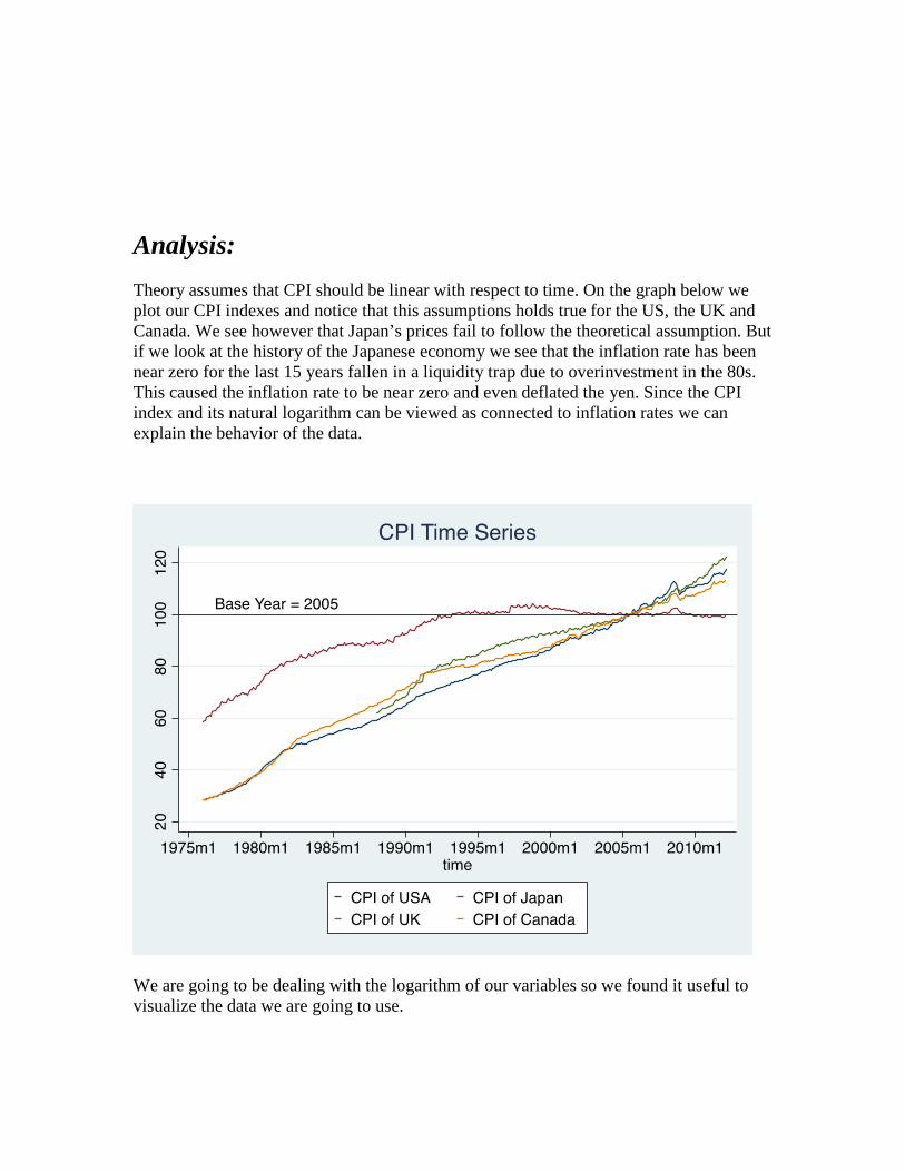
Analysis: Theory assumes that CPI should be linear with respect to time. On the graph below we plot our CPI indexes and notice that this assumptions holds true for the US, the UK and Canada. We see however that Japan’s prices fail to follow the theoretical assumption. But if we look at the history of the Japanese economy we see that the inflation rate has been near zero for the last 15 years fallen in a liquidity trap due to overinvestment in the 80s. This caused the inflation rate to be near zero and even deflated the yen. Since the CPI index and its natural logarithm can be viewed as connected to inflation rates we can explain the behavior of the data.

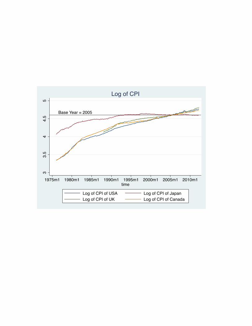
We are going to be dealing with the logarithm of our variables so we found it useful to visualize the data we are going to use.

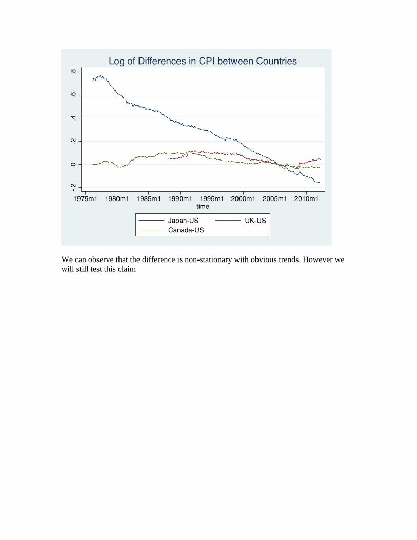
We can observe that the difference is non-stationary with obvious trends. However we will still test this claim

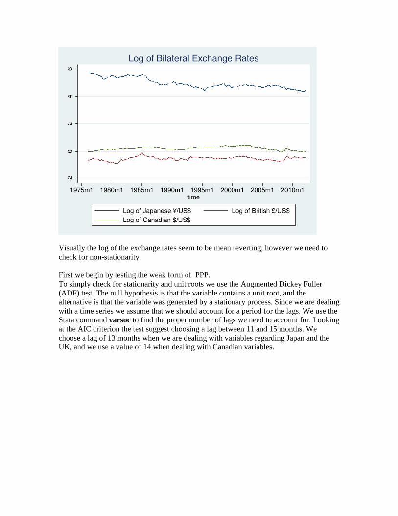
Visually the log of the exchange rates seem to be mean reverting, however we need to check for non-stationarity. First we begin by testing the weak form of PPP. To simply check for stationarity and unit roots we use the Augmented Dickey Fuller (ADF) test. The null hypothesis is that the variable contains a unit root, and the alternative is that the variable was generated by a stationary process. Since we are dealing with a time series we assume that we should account for a period for the lags. We use the Stata command varsoc to find the proper number of lags we need to account for. Looking at the AIC criterion the test suggest choosing a lag between 11 and 15 months. We choose a lag of 13 months when we are dealing with variables regarding Japan and the UK, and we use a value of 14 when dealing with Canadian variables.

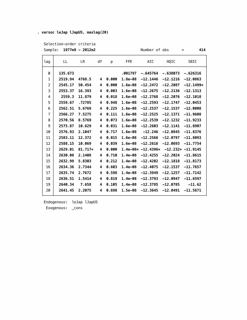
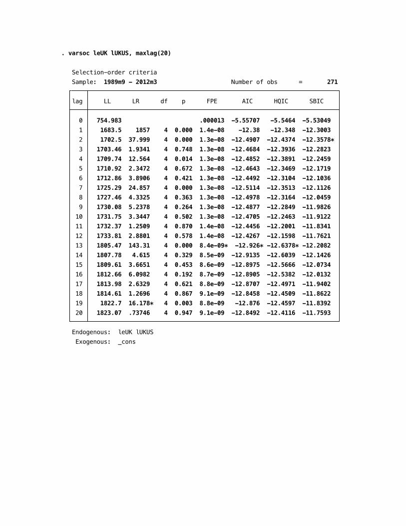
Note that we assume that theory suggests exchange rates take a long time to adjust/change (approximately a year or so) that is why we choose the max lags to be 20. Once we have chosen the number of lags we should account for we are free to proceed with the chosen ADF test.

We see from the ADF that we fail to reject the null hypothesis that there are no unit roots over all of the countries in our sample. Thus it is plausible to assume cointegration. This means that long term convergence to PPP is possible. Another method we use to check for cointegration between a pair of currencies is the Engle-Granger test:

We cannot reject the null hypothesis of no unit roots thus an assumption of non-stationarity is plausible.

We cannot reject the null hypothesis of no unit roots thus an assumption of non-stationarity is plausible.

We cannot reject the null hypothesis of no unit roots thus an assumption of non-stationarity is plausible.

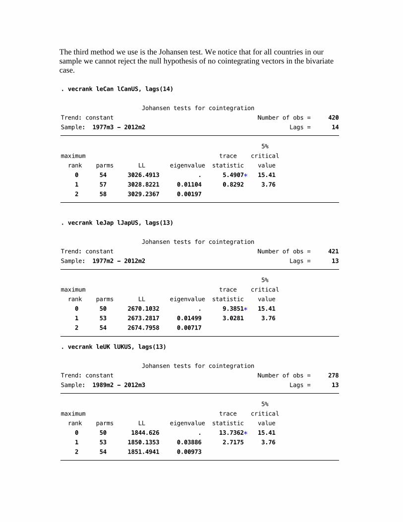
The third method we use is the Johansen test. We notice that for all countries in our sample we cannot reject the null hypothesis of no cointegrating vectors in the bivariate case.

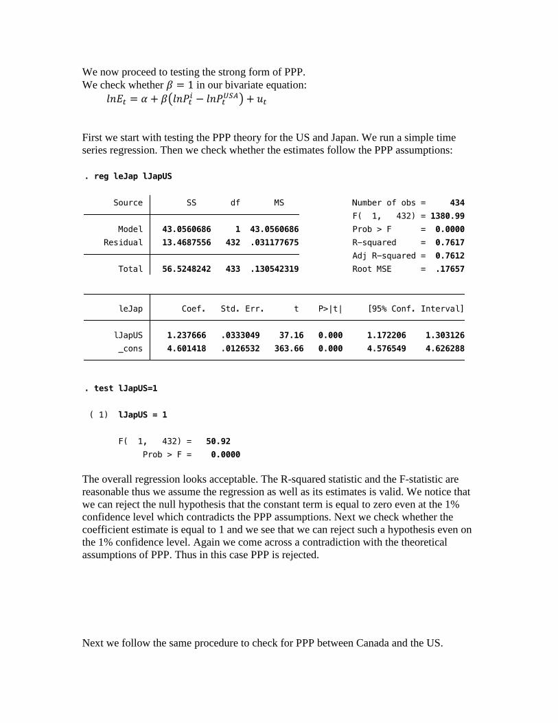
We now proceed to testing the strong form of PPP. We check whether 𝛽 = 1 in our bivariate equation: 𝑙𝑛𝐸𝑡 = 𝛼 + 𝛽�𝑙𝑛𝑃𝑡𝑖 − 𝑙𝑛𝑃𝑡𝑈𝑆𝐴� + 𝑢𝑡 First we start with testing the PPP theory for the US and Japan. We run a simple time series regression. Then we check whether the estimates follow the PPP assumptions:

The overall regression looks acceptable. The R-squared statistic and the F-statistic are reasonable thus we assume the regression as well as its estimates is valid. We notice that we can reject the null hypothesis that the constant term is equal to zero even at the 1% confidence level which contradicts the PPP assumptions. Next we check whether the coefficient estimate is equal to 1 and we see that we can reject such a hypothesis even on the 1% confidence level. Again we come across a contradiction with the theoretical assumptions of PPP. Thus in this case PPP is rejected. Next we follow the same procedure to check for PPP between Canada and the US.

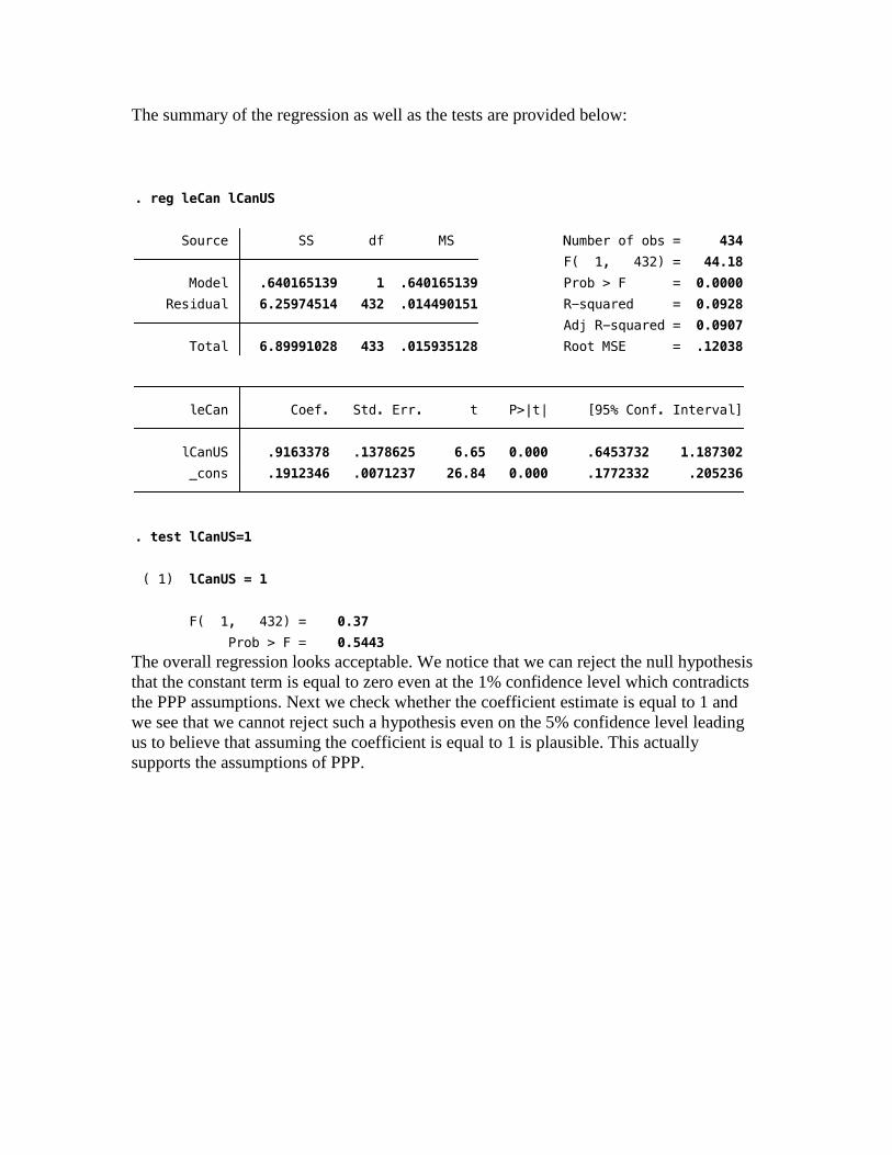
The summary of the regression as well as the tests are provided below:

The overall regression looks acceptable. We notice that we can reject the null hypothesis that the constant term is equal to zero even at the 1% confidence level which contradicts the PPP assumptions. Next we check whether the coefficient estimate is equal to 1 and we see that we cannot reject such a hypothesis even on the 5% confidence level leading us to believe that assuming the coefficient is equal to 1 is plausible. This actually supports the assumptions of PPP.

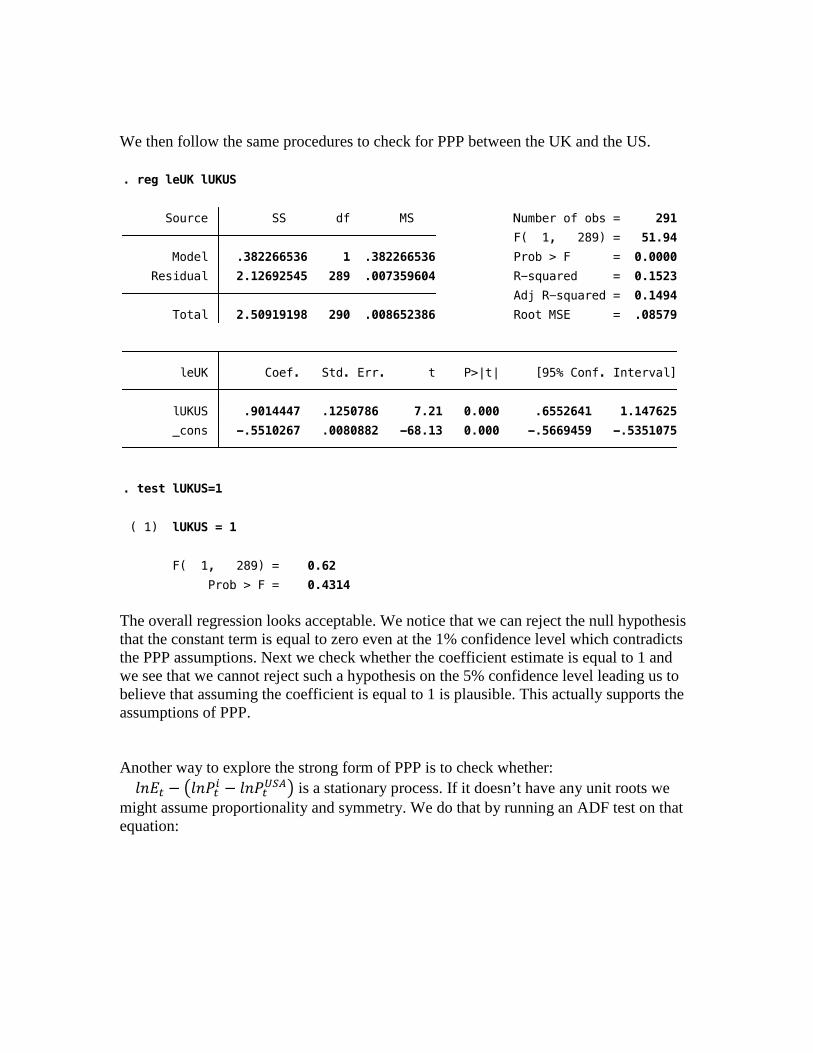
We then follow the same procedures to check for PPP between the UK and the US.

The overall regression looks acceptable. We notice that we can reject the null hypothesis that the constant term is equal to zero even at the 1% confidence level which contradicts the PPP assumptions. Next we check whether the coefficient estimate is equal to 1 and we see that we cannot reject such a hypothesis on the 5% confidence level leading us to believe that assuming the coefficient is equal to 1 is plausible. This actually supports the assumptions of PPP. Another way to explore the strong form of PPP is to check whether: 𝑙𝑛𝐸𝑡 − �𝑙𝑛𝑃𝑡𝑖 − 𝑙𝑛𝑃𝑡𝑈𝑆𝐴� is a stationary process. If it doesn’t have any unit roots we might assume proportionality and symmetry. We do that by running an ADF test on that equation:

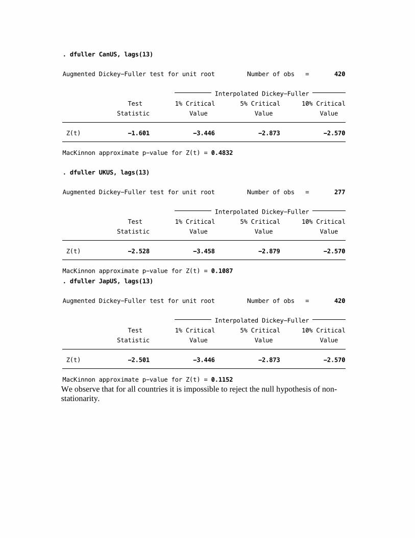
We observe that for all countries it is impossible to reject the null hypothesis of non-stationarity.

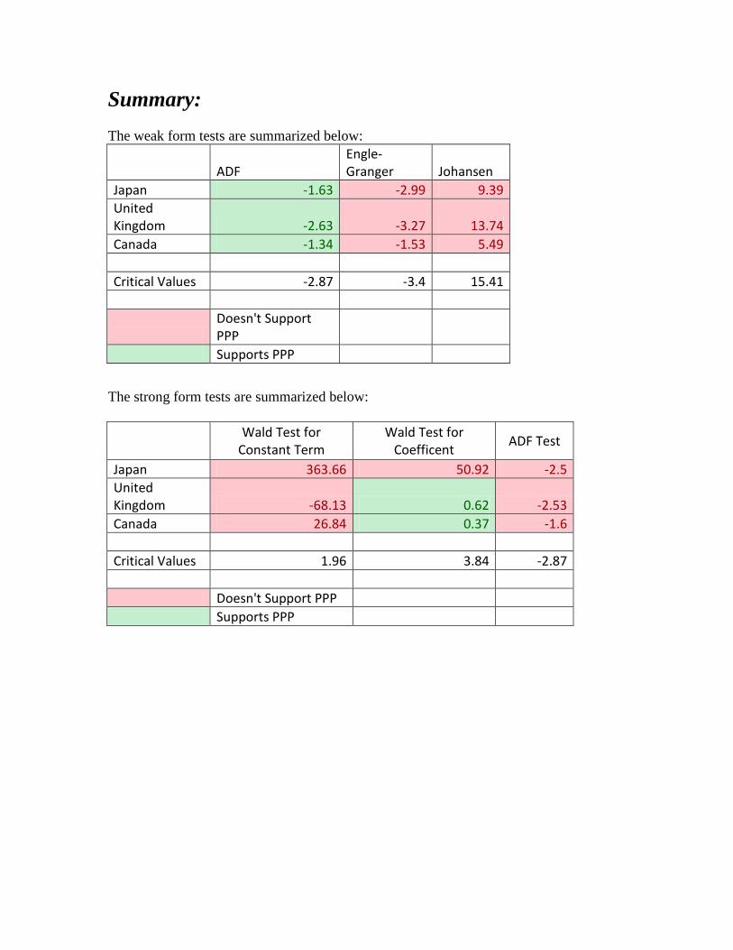
Summary: The weak form tests are summarized below:

ADF Engle-Granger Johansen

Japan -1.63 -2.99 9.39 United Kingdom -2.63 -3.27 13.74 Canada -1.34 -1.53 5.49 Critical Values -2.87 -3.4 15.41

Doesn't Support PPP

Supports PPP

The strong form tests are summarized below:

Wald Test for

Constant Term Wald Test for

Coefficent ADF Test

Japan 363.66 50.92 -2.5 United Kingdom -68.13 0.62 -2.53 Canada 26.84 0.37 -1.6 Critical Values 1.96 3.84 -2.87 Doesn't Support PPP Supports PPP

Conclusion: Purchasing power parity has been one of the more puzzling concepts in economics ever since the theory was first introduced by Prof Cassel in the early 20th century. In this project we try to find evidence of both the weak and the strong form of PPP. We find very little support for the weak form of PPP. The tests in favor of the doctrine are very weak in nature and thus non-conclusive. We find enough evidence to firmly reject the strong form for all of the countries in our sample. There is absolutely no evidence for symmetry or proportionality in our cointegration tests. Some have suggested that deviation from the PPP norm could be cause by interaction between the real exchange rates and real domestic interest rates. This is suggested by Johansen and Juselius (1990b). Other reasons for inconsistencies with the PPP theory might include level of output, GDP growth, money supply, etc. Diebold and Rudebusch (1989) and Shea (1991) are among of the articles dealing with such factors. We also must account for the fact that there is rarely perfect mobility between economic entities. Transaction costs (taxes tariffs, etc.) might also lead to inefficiencies that in turn should cause deviation from the PPP doctrine. A better and more detailed price indicator will be helpful in further exploring the theory.