Waveforms for the Massive MIMO Downlink: Amplifier Efficiency, Distortion and

Performance

Christopher Mollén, Erik G. Larsson and Thomas Eriksson

Linköping University Post Print

N.B.: When citing this work, cite the original article.

©2016 IEEE. Personal use of this material is permitted. However, permission to reprint/republish this material for advertising or promotional purposes or for creating new collective works for resale or redistribution to servers or lists, or to reuse any copyrighted component of this work in other works must be obtained from the IEEE.

Christopher Mollén, Erik G. Larsson and Thomas Eriksson, Waveforms for the Massive MIMO Downlink: Amplifier Efficiency, Distortion and Performance, 2016, IEEE Transactions on Communications, 99, 1-1. http://dx.doi.org/10.1109/TCOMM.2016.2557781 Postprint available at: Linköping University Electronic Press

http://urn.kb.se/resolve?urn=urn:nbn:se:liu:diva-130514

1

Waveforms for the Massive MIMO Downlink:Amplifier Efficiency, Distortion and Performance

Christopher Mollen, Erik G. Larsson and Thomas Eriksson

Abstract—In massive MIMO, most precoders result in downlinksignals that suffer from high PAR, independently of modulationorder and whether single-carrier or OFDM transmission is used.The high PAR lowers the power efficiency of the base stationamplifiers. To increase power efficiency, low-PAR precoders havebeen proposed. In this article, we compare different transmissionmethods for massive MIMO in terms of the power consumedby the amplifiers. It is found that: 1) OFDM and single-carriertransmission have the same performance over a hardened massiveMIMO channel and 2) when the higher amplifier power efficiencyof low-PAR precoding is taken into account, conventional andlow-PAR precoders lead to approximately the same power con-sumption. Since downlink signals with low PAR allow for simplerand cheaper hardware, than signals with high PAR, therefore, theresults suggest that low-PAR precoding with either single-carrieror OFDM transmission should be used in a massive MIMO basestation.

Index Terms—low-PAR precoding, massive MIMO, multiuserprecoding, out-of-band radiation, peak-to-average ratio, poweramplifier, power consumption.

I. INTRODUCTION

W IRELESS massive MIMO (Multiple-Input Multiple-Output) systems, initially conceived in [2] and popularly

described in [3], simultaneously serve tens of users with basestations equipped with tens or hundreds of antennas usingmultiuser precoding. Compared to classical multiuser MIMO,order-of-magnitude improvements are obtained in spectraland energy efficiency [4], [5]. For these reasons, massiveMIMO is expected to be a key component of future wirelesscommunications infrastructure [3], [6].

This work compares different multiuser precoding techniquesfor the massive MIMO downlink. Under a total radiated powerconstraint, optimal multiuser MIMO precoding is a rather well-understood topic, see, e.g., [7], [8], as is linear (and necessarilysuboptimal) precoding, see, e.g., [9] and the survey [10]. Itis also known that, for massive MIMO specifically, linearprecoding is close to optimal under a total-radiated powerconstraint [5]. There are also numerous results on precodingunder per-antenna power constraints [11]–[13].

In practice, massive MIMO precoders optimized subject toa total radiated power constraint yield transmit signals with

C. Mollen and E. Larsson are with the Communication Systems Division,Dept. of Electrical Eng. (ISY), Linkoping University, Linkoping, Sweden, andT. Eriksson is with the Dept. of Signals and Systems, Chalmers University ofTechnology, Gothenburg, Sweden.

The research leading to these results has received funding from the Euro-pean Union Seventh Framework Programme under grant agreement numberICT-619086 (MAMMOET), the Swedish Research Council (Vetenskapsradet)and ELLIIT.

Parts of this work were presented at the European Wireless conference 2014[1].

NormalizedFInstantaneousFPowerF|x(t)|2/E[|x(t)|]2 [dB]

-2 0 2 4 6 8 10 12

CC

DF

10-8

10-6

10-4

10-2

100

single-carrierFzero-forcing,F4-QAM

OFDMFzero-forcing,FGauss

low-PARFprecoding

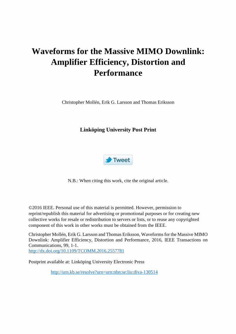
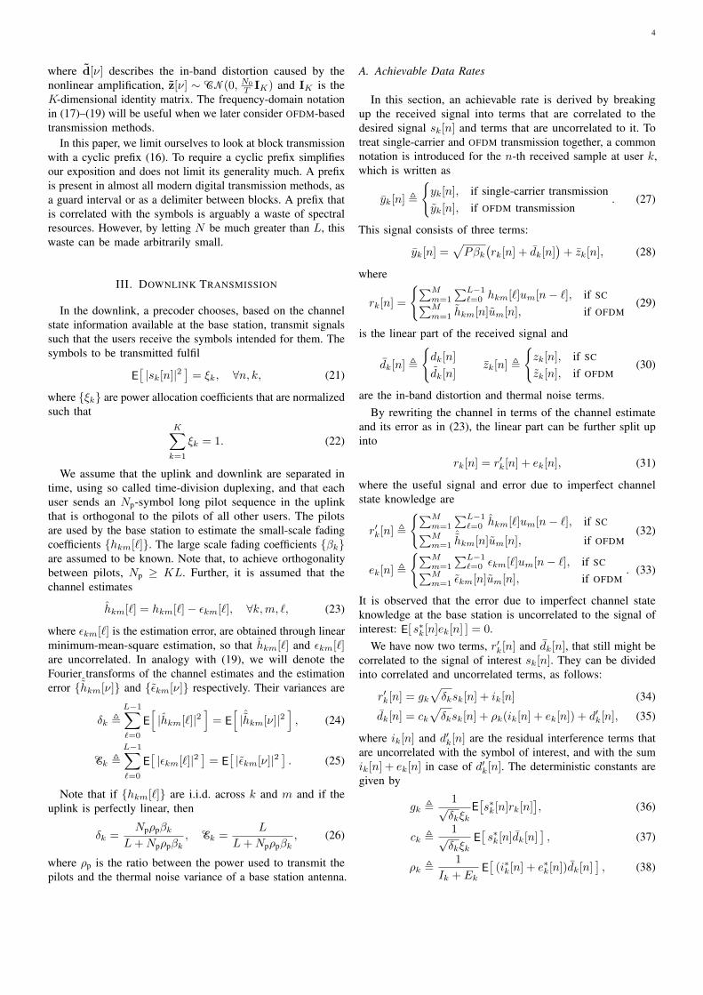
Fig. 1. The complimentary cumulative distribution of the amplitudes ofdifferent massive MIMO downlink signals that have been pulse shaped by a root-raised cosine filter, roll-off 0.22. Single-carrier and OFDM transmission havevery similar distributions for the linear precoders described in Section III-B3for any modulation order, cf. [15]. The low-PAR precoding technique is theone described in [16] and in Section III-C1. The system has 100 base stationantennas, 10 single-antenna users and the channel is i.i.d. Rayleigh fadingwith 4 taps.

high peak-to-average ratio (PAR), regardless of whether single-carrier or orthogonal frequency-division multiplexing (OFDM)transmission and of whether a low or a high modulation orderis used, see Figure 1. To avoid heavy signal distortion andout-of-band radiation, transmission of such signals requiresthat the power amplifiers are backed off and operated at apoint, where their transfer characteristics are sufficiently linear[14]. The higher the signal PAR is, the more backoff is needed;and the higher the backoff is, the lower the power efficiencyof the amplifier will be. Against this background, precodersthat yield signals with low PAR would be desirable.

The possibility to perform low-PAR precoding is a uniqueopportunity offered by the massive MIMO channel—signalpeaks can be reduced because the massive MIMO downlinkchannel has a large nullspace and any additional signaltransmitted in the nullspace does not affect what the usersreceive. In particular, PAR-reducing signals from the channelnullspace can be added to the downlink signal so that theemitted signals have low PAR [3], [17]. A few low-PARprecoders for massive MIMO have been proposed in theliterature [16]–[18]. In [17], the discrete-time downlink signalswere constrained to have constant envelopes.1 There it wasestimated that, in typical massive MIMO scenarios, 1–2 dBextra radiated power is required to achieve the same sum-rateas without an envelope constraint. While some extra radiatedpower is required by low-PAR precoders, it was argued in [17]

1Note that the precoder in [17] can transmit symbols from any generalinput constellation and is compatible with both single-carrier transmission andOFDM—the received signals do not have to have constant envelopes, only thedownlink signal emitted from each base station antenna has constant envelope.

2

that the overall power consumption still should decrease dueto the increased amplifier efficiency.

Another unique feature of the massive MIMO downlinkchannel is that certain types of hardware-induced distortiontend to average out when observed at the receivers [19]. Ourstudy confirms that the variance of the in-band distortion causedby nonlinear base station amplifiers does decrease with thenumber of base station antennas.

Because the amount of power dissipation from the amplifiersdepends on the amplitude distribution of the transmit signals,and because different transmit signals considered for massiveMIMO systems have widely different amplitude distributions(widely different PAR), it is important to evaluate their per-formance in terms of the amount of power consumed by theamplifiers rather in terms of the amount of power that isradiated. The paper at hand compares precoders with differentamplitude distributions in terms of amplifier power consumptionand quantifies the benefits of low-PAR precoding for the massiveMIMO downlink, taking into account in-band distortion andout-of-band radiation stemming from amplifier nonlinearitiesand imperfect channel state information due to pilot-basedchannel estimation. To the best knowledge of the authors, acomprehensive comparison, where amplifier efficiency anddistortion are functions of the specific input signal rather thansimplified functions of PAR, has not been done before. Thedifference between OFDM and single-carrier transmission isalso investigated. The main technical contribution of the paperis a comprehensive end-to-end modeling of massive MIMOdownlink transmission, which is treated in continuous timein order to capture the effects of nonlinear amplification, theassociated capacity bound, and the estimations of the powerconsumption for relevant amplifier models. All conclusions aresummarized in Section V.

We stress that the effect of amplifier nonlinearities onwireless signals have also been studied by others [14], [20],and for MIMO specifically in [21]. In relation to this literature,the novel aspects of our work include: (i) a specific focus onthe massive MIMO downlink channel, which facilitates low-PARprecoding; (ii) a classification and comparison of precoderscommonly considered for massive MIMO; (iii) an estimate ofthe amplifier power consumption of low-PAR precoding incomparison to that of other standard precoders.

II. SYSTEM MODEL

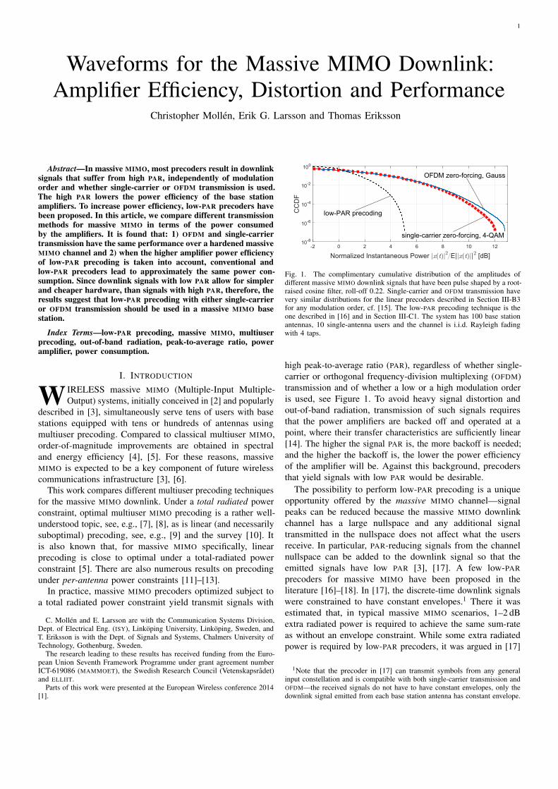
The downlink shown in Figure 2(a) is studied. The basestation is equipped with M antennas and it serves K single-antenna users over a frequency-selective channel. All signalsare modeled in complex baseband.

We let sk[n] be the n-th symbol that is to be transmitted touser k and collectively denote all the n-th symbols by s[n] ,(s1[n], . . . , sK [n]). The base station precodes the symbols toproduce the discrete-time signals {um[n]}, where um[n] is theprecoded signal of antenna m. These signals are scaled suchthat

M∑m=1

E[|um[n]|2

]= 1, ∀n (1)

Precoder

u1[n]p(τ) P

uM[n]cont. channel

{H[ℓ]}

PUser k

yk[n]p*(−τ)s[n]

u1(t)

uM(t)

x1(t)

xM(t)p(τ)

βkh

k1(τ)

βkhkM(τ)

yk(t)

(a) The continuous-time model of the downlink.

Precoder

u1[n]

uM[n]disc. channel

{H[ℓ]}

User k

yk[n]s[n]

P

P

dk[n]+zk[n]

βkhk1[n]

βkhkM[n]

(b) The equivalent discrete-time model of the downlink.

Fig. 2. The downlink of a massive MIMO system.

and pulse shaped by a filter with impulse response p(τ) intothe continuous-time transmit signals

um(t) ,∑n

um[n]p(t− nT ), (2)

where T is the symbol period. After pulse shape filtering, thetransmit signal um(t) has a bandwidth smaller or equal to thebandwidth B of the pulse p(τ). The bandwidth B is the widthof the interval, over which the spectrum of p(τ) is non-zero.For example, if a root-raised cosine filter of period T withroll-off σ were used, then BT = 1 + σ.

The continuous-time signal um(t) is then amplified totransmit power by an amplifier that, in general, is nonlinear.The amplified signal is given by

xm(t) = g( |um(t)|√

b

)ej(arg um(t)+Φ(|um(t)|/

√b)), (3)

where g(|um(t)|) is the AM-AM conversion and Φ(|um(t)|)the AM-PM conversion2, see for example [15]. For now, theconversions g(u) and Φ(u) are generic functions. Later in ouranalysis however, appropriate assumptions will be made tospecify them. The factor b is the backoff that has to be done toavoid nonlinear amplification and distortion. By backing off thesignal power to a suitable operating point, the signal amplitudewill stay in a region with sufficiently linear amplification mostof the time, see [15]. In this article, all backoffs are given indB relative to the backoff of the 1-dB compression point—thepoint, where the output signal is 1 dB weaker than what itwould have been if the amplification were perfectly linear. Thesignals are amplified so that

limt0→∞

M∑m=1

E

[1

t0

t0/2∫−t0/2

|xm(t)|2dt

]= P, (4)

where P is the transmitted power of the base station.The nonlinear relation in (3) generally widens the spectrum

2The acronyms in the terms AM-AM and AM-PM conversion stand for thefact that these functions describe how the modulation of the amplitude affectsthe Amplitude Modulation and Phase Modulation of the amplified signal.

3

0 0.5 1 1.5 2−70

−60

−50

−40

−30

−20

−10

0

10

Pow

erqS

pect

ralqD

ensi

tyq[d

B]

Frequency fT

PAOoperationOatO1dBOcompression

10 dBOback-off

InOband RightOband

low-PAROprecodedOsingle-carrier

Maximum-ratioOprecodedOOFDM

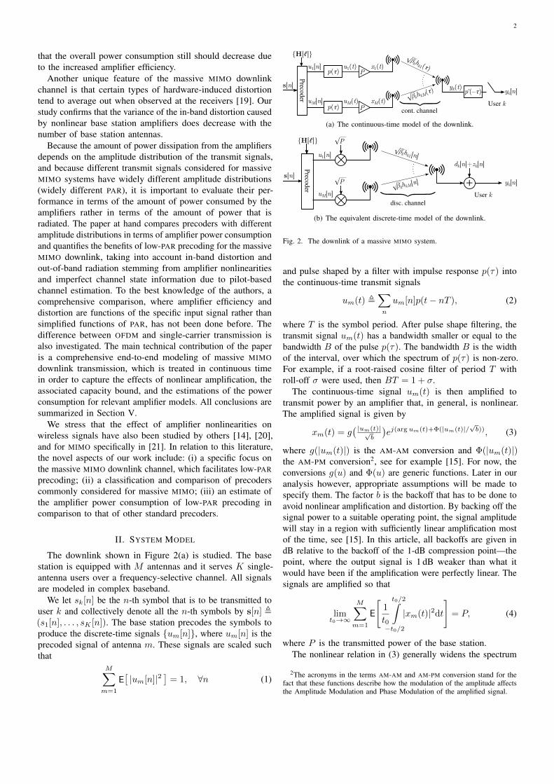
Fig. 3. The power spectral densities after amplification of two signal typeswith the PA operating at the 1 dB compression point (upper two curves) andwell below saturation (lower two curves). The signals are from the system laterdescribed in Table I, where the bandwidth of the pulse p(τ) is BT = 1.22.

of the amplified signal, i.e. the power of the signal is no longerconfined to the bandwidth B of the pulse p(τ). The poweroutside the ideal bandwidth is called out-of-band radiation andis quantified by the adjacent channel leakage ratio (ACLR),which is defined in terms of the power P[−B/2,B/2] of xm(t)in the useful band and the powers P[−3B/2,−B/2], P[B/2,3B/2]

in the immediately adjacent bands:

ACLR , max

(P[−3B/2,−B/2]

P[−B/2,B/2],P[B/2,3B/2]

P[−B/2,B/2]

), (5)

where

PB ,∫f∈B

Sx(f)df. (6)

and Sx(f) is the power spectral density of xm(t). In Figure 3,four power spectral densities of different amplified signals areshown to illustrate the out-of-band radiation. Half the in-bandspectrum is shown together with the whole right band.

This signal is broadcast over the channel, whose small-scalefading impulse response from antenna m to user k is hkm(τ)and large-scale fading coefficient to user k is βk. Specifically,user k receives the signal

yk(t) =√βk

M∑m=1

(hkm(τ) ? xm(τ)

)(t) + zk(t), (7)

where zk(t) is a stationary white Gaussian stochastic processwith spectral height N0 that models the thermal noise of theuser equipment. The received signal is passed through a filtermatched to the pulse p(τ) and sampled to produce the discrete-time received signal

yk[n] ,(p∗(−τ) ? yk(τ)

)(nT ). (8)

In analyzing this system, we will look into an equivalentdiscrete-time system, see Figure 2(b). In order to do that, thedistortion produced by the nonlinear amplifier has to be treatedseparately, since the nonlinearity widens the spectrum and isnot accurately described by symbol-rate sampling. The small-scale fading coefficients of the discrete-time impulse responseof the channel, including the pulse-shaping and matched filter,between antenna m and user k are denoted

hkm[`] , T(p(τ) ? hkm(τ) ? p∗(−τ)

)(`T ). (9)

For these channel coefficients, we assume that

E[h∗km[`]hkm[`′] ] = 0, ∀` 6= `′, (10)

L−1∑`=0

E[|hkm[`]|2

]= 1, ∀k,m, (11)

and that hkm[`] is zero for integers ` /∈ [0, L−1], where L isthe number of channel taps.

The n-th received sample at user k is then given by

yk[n] =√Pβk

( M∑m=1

L−1∑`=0

hkm[`]um[n−`] + dk[n])+ zk[n],

(12)

where the noise sample zk[n] ,(p∗(−τ) ? zk(τ)

)(nT ). To

make zk[n] ∼ CN(0, N0/T ) i.i.d., it is assumed that p(τ) is aroot-Nyquist pulse of period T and signal energy 1/T . The termdk[n] describes the in-band distortion—the part of the distortionthat can be seen in the received samples yk[n]—caused by thenonlinear amplification of the transmit signal. It is given bydk[n] ,

1√P

M∑m=1

((xm(t)−

√Pum(t)

)? hkm(τ) ? p∗(−τ)

)(nT ). (13)

By introducing the following vectors

u[n] , (u1[n], . . . , uM [n])T y[n] , (y1[n], . . . , yK [n])T

d[n] , (d1[n], . . . , dK [n])T z[n] , (z1[n], . . . , zK [n])T

and matrices

H[`],

h11[`] · · · h1M [`]...

. . ....

hK1[`] · · · hKM [`]

B,diag(β1, . . . , βK), (14)

the received signals can be written as

y[n] =√PB

12

(L−1∑`=0

H[`]u[n− `] + d[n])+ z[n]. (15)

If the transmission were done in a block of N symbols peruser, and a cyclic prefix were used in front of the blocks, i.e.

u[n] = u[N + n], for n = −L+ 1, . . . ,−1, (16)

where n = 0 is the time instant when the first symbol is receivedat the users, then the received signal in (15) is easily given inthe frequency domain. If the discrete Fourier transforms of thetransmit signals, received signals and channel are denoted by

u[ν] ,N−1∑n=0

e−j2πnν/Nu[n], (17)

y[ν] ,N−1∑n=0

e−j2πnν/Ny[n], (18)

H[ν] ,L−1∑`=0

e−j2π`ν/NH[`], (19)

then the received signal at frequency index ν is given by

y[ν] =√PB

12

(H[ν]u[ν] + d[ν]

)+ z[ν], (20)

4

where d[ν] describes the in-band distortion caused by thenonlinear amplification, z[ν] ∼ CN(0, N0

T IK) and IK is theK-dimensional identity matrix. The frequency-domain notationin (17)–(19) will be useful when we later consider OFDM-basedtransmission methods.

In this paper, we limit ourselves to look at block transmissionwith a cyclic prefix (16). To require a cyclic prefix simplifiesour exposition and does not limit its generality much. A prefixis present in almost all modern digital transmission methods, asa guard interval or as a delimiter between blocks. A prefix thatis correlated with the symbols is arguably a waste of spectralresources. However, by letting N be much greater than L, thiswaste can be made arbitrarily small.

III. DOWNLINK TRANSMISSION

In the downlink, a precoder chooses, based on the channelstate information available at the base station, transmit signalssuch that the users receive the symbols intended for them. Thesymbols to be transmitted fulfil

E[|sk[n]|2

]= ξk, ∀n, k, (21)

where {ξk} are power allocation coefficients that are normalizedsuch that

K∑k=1

ξk = 1. (22)

We assume that the uplink and downlink are separated intime, using so called time-division duplexing, and that eachuser sends an Np-symbol long pilot sequence in the uplinkthat is orthogonal to the pilots of all other users. The pilotsare used by the base station to estimate the small-scale fadingcoefficients {hkm[`]}. The large scale fading coefficients {βk}are assumed to be known. Note that, to achieve orthogonalitybetween pilots, Np ≥ KL. Further, it is assumed that thechannel estimates

hkm[`] = hkm[`]− εkm[`], ∀k,m, `, (23)

where εkm[`] is the estimation error, are obtained through linearminimum-mean-square estimation, so that hkm[`] and εkm[`]are uncorrelated. In analogy with (19), we will denote theFourier transforms of the channel estimates and the estimationerror {ˆhkm[ν]} and {εkm[ν]} respectively. Their variances are

δk ,L−1∑`=0

E[|hkm[`]|2

]= E

[|ˆhkm[ν]|2

], (24)

Ek ,L−1∑`=0

E[|εkm[`]|2

]= E

[|εkm[ν]|2

]. (25)

Note that if {hkm[`]} are i.i.d. across k and m and if theuplink is perfectly linear, then

δk =Npρpβk

L+Npρpβk, Ek =

L

L+Npρpβk, (26)

where ρp is the ratio between the power used to transmit thepilots and the thermal noise variance of a base station antenna.

A. Achievable Data Rates

In this section, an achievable rate is derived by breakingup the received signal into terms that are correlated to thedesired signal sk[n] and terms that are uncorrelated to it. Totreat single-carrier and OFDM transmission together, a commonnotation is introduced for the n-th received sample at user k,which is written as

yk[n] ,

{yk[n], if single-carrier transmissionyk[n], if OFDM transmission

. (27)

This signal consists of three terms:

yk[n] =√Pβk

(rk[n] + dk[n]

)+ zk[n], (28)

where

rk[n] =

{∑Mm=1

∑L−1`=0 hkm[`]um[n− `], if SC∑M

m=1 hkm[n]um[n], if OFDM(29)

is the linear part of the received signal and

dk[n] ,

{dk[n]

dk[n]zk[n] ,

{zk[n], if SC

zk[n], if OFDM(30)

are the in-band distortion and thermal noise terms.By rewriting the channel in terms of the channel estimate

and its error as in (23), the linear part can be further split upinto

rk[n] = r′k[n] + ek[n], (31)

where the useful signal and error due to imperfect channelstate knowledge are

r′k[n] ,

{∑Mm=1

∑L−1`=0 hkm[`]um[n− `], if SC∑M

m=1ˆhkm[n]um[n], if OFDM

(32)

ek[n] ,

{∑Mm=1

∑L−1`=0 εkm[`]um[n− `], if SC∑M

m=1 εkm[n]um[n], if OFDM. (33)

It is observed that the error due to imperfect channel stateknowledge at the base station is uncorrelated to the signal ofinterest: E[ s∗k[n]ek[n] ] = 0.

We have now two terms, r′k[n] and dk[n], that still might becorrelated to the signal of interest sk[n]. They can be dividedinto correlated and uncorrelated terms, as follows:

r′k[n] = gk√

δksk[n] + ik[n] (34)

dk[n] = ck√δksk[n] + ρk(ik[n] + ek[n]) + d′k[n], (35)

where ik[n] and d′k[n] are the residual interference terms thatare uncorrelated with the symbol of interest, and with the sumik[n] + ek[n] in case of d′k[n]. The deterministic constants aregiven by

gk ,1√δkξk

E[s∗k[n]rk[n]

], (36)

ck ,1√δkξk

E[s∗k[n]dk[n]

], (37)

ρk ,1

Ik + EkE[(i∗k[n] + e∗k[n])dk[n]

], (38)

5

where the channel error and interference variances are

Ek , E[|ek[n]|2

], (39)

Ik , E[|ik[n]|2

]. (40)

We note that, when (26) holds, Ek = Ek. The factors gk andck are normalized by

√δk so that they do not depend on the

estimation error δk. This normalization will later allow us tosee the impact of the channel estimation error on the SINR.The fact that gk does not depend on δk is seen by expandinggk as is done in (84) in the Appendix. The interference ik[n]is uncorrelated with sk[n] because

E[ s∗k[n]ik[n] ] = E[s∗k[n](rk[n]− gkδ

12

k sk[n])]

= E[s∗k[n]rk[n]

]− gkδ

12

k ξk = 0. (41)

That d′k[n] is uncorrelated with both sk[n] and ik[n]+ek[n] canbe shown in the same way. The factor ck should be interpretedas the amount of amplitude that the nonlinear amplification“contributes” to the amplitude of the signal of interest. Usually,in a real-world system, this is a negative contribution in thesense that |gk + ck| < |gk|. It should therefore be seen as theamount of amplitude lost (in what is usually called clipping).Similarly, the other correlation ρk is the amount of interferencethat is clipped by the nonlinear amplification.

The whole received signal can thus be given as the sum ofthe following terms

yk[n] =√Pβk

(√δk(gk+ck)sk[n]

+ (1 + ρk)(ik[n] + ek[n]) + d′k[n])+ zk[n] (42)

A lower bound3 on the capacity of the downlink channel touser k is given by [22], [23]

Rk, log2 (1 + SINRk) , (43)

where the signal-to-interference-and-noise ratio (SINR) is givenby

SINRk =|E[ y∗k[n]sk[n] ] |2/ξk

E[ |yk[n]|2 ]− |E[ y∗k[n]sk[n] ] |2/ξk. (44)

Note that the capacity bound in (43) makes no assumptionon Gaussianity of the interference terms. Further, it is not afunction of the data symbols, only their second-order statistics.

To evaluate the expectations, we denote the variance of thein-band distortion

Dk , E[|d′k[n]|2

]. (45)

With this new notation, the two expectations in (44) can bewritten as follows.

|E[ y∗k[n]sk[n] ] |2/ξk = δkξkPβk|gk + ck|2 (46)

E[|yk[n]|2

]= Pβk(δkξk|gk+ck|2

+ (Ik+Ek)|1+ρk|2+Dk)+N0

T (47)

3This analysis is general and does not make any assumption on Gaussianityof the transmit signals. In the computation of the capacity bound, however,a Gaussian distribution is used as one of the permissible distributions; itsinsertion into the expression for the mutual information yields a lower boundon capacity.

This simplifies (44), which becomes

SINRk =δkξkPβk|gk + ck|2

Pβk

((Ik+Ek)|1+ρk|2+Dk

)+N0

T

. (48)

From (48), the two consequences of nonlinear amplificationcan be seen: (i) in-band distortion with variance Dk and (ii)signal clipping by ck, a reduction of the signal amplitude thatresults in a power-loss.

We also see that the variance δk is the fraction between thepower that would have been received if the channel estimateswere perfect and the actually received power. It can thus beseen as a measure of how much power that is lost due toimperfect channel state information at the base station.

The bound (43) is an achievable rate of a system thatuses a given precoder and where the detector uses (36) as achannel estimate and treats the error terms in (42) as additionaluncorrelated Gaussian noise. This detector has proven to beclose to the optimal detector in environments, where themassive MIMO channel hardens.

B. Linear Precoding Techniques

With knowledge of the channel, the base station can precodethe symbols in such a way that the gain gk is large and theinterference Ik small.

1) OFDM-Transmission: In OFDM transmission, the pre-coder is defined in the frequency domain. The time domaintransmit signals are obtained from the inverse Fourier transform

u[n] ,N−1∑ν=0

ej2πnν/N u[ν] (49)

of the precoded signals

u[ν] = W[ν]s[ν], ν = 1, . . . , N−1 (50)

where W[ν] is a precoding matrix for frequency ν. Theprecoding is linear, because the precoding matrix does notdepend on the symbols, only on the channel.

To ensure that (1) is fulfilled, it is required that

E[‖W[ν]‖2F

]= K, ∀ν. (51)

2) Single-Carrier Transmission: The transmit signals ofsingle-carrier transmission are given by the cyclic convolution

u[n] =

N−1∑`=0

W[`]s[n− `], (52)

where the indices are taken modulo N . The impulse responseof the precoder is given in terms of its frequency domaincounterpart:

W[`] ,N−1∑ν=0

ej2πν`/NW[ν]. (53)

3) Conventional Precoders: In this paper, three conventionalprecoders are studied. They will be given as functions of thechannel estimates {H[`]} (a sequence of matrices defined in

6

terms of {hkm[`]} in the same way as H[`] is defined in (14)in terms of {hkm[`]}) and its Fourier transform

ˆH[ν] ,N−1∑`=0

H[`]e−j2πν`/N . (54)

a) Maximum-Ratio Precoding: Maximum-ratio precodingis the precoder that maximizes the gain gk and the receivedpower of the desired signal. It is given by

W[ν] = αMRˆH

H[ν], for MR, (55)

where αMR is a power normalization factor that is chosen suchthat (51) holds. For maximum-ratio precoding

α2MR =

1

M∑K

k=1 δk. (56)

While it maximizes the received power of the transmission,interference Ik 6= 0 is still present in the received signal. Intypical scenarios with favorable propagation, maximum-ratioprecoding suppresses this interference increasingly well withhigher number of base station antennas and in the limit ofinfinitely many antennas, the interference becomes negligiblein comparison to the received power [2]. For maximum-ratioprecoding and an i.i.d. Rayleigh fading channel, both withsingle-carrier and OFDM transmission, the array gain andinterference terms are [5]

gk =√M, Ik = δk, for MR.

Because the precoding weights of antenna m only depend onthe channel coefficients {hkm[`]} of that antenna, maximum-ratio precoding can be implemented in a distributed fashion,where the precoding is done locally at each antenna.

Note that this definition of maximum-ratio precoding makesit equivalent to time-reversal precoding for single-carriertransmission, see for example [24].

b) Zero-Forcing Precoding: The zero-forcing precoder isgiven by

W[ν] = αZFˆH

H[ν]

( ˆH[ν] ˆHH[ν]

)−1, for ZF, (57)

where αZF is a power normalization factor that is chosen suchthat (51) holds. For zero-forcing precoding

αZF =M −K∑K

k=11δk

, (58)

in the derivation of which we used the fact [25] that

E[∥∥HH[ν]

(H[ν]HH[ν]

)−1∥∥2] = E[tr(H[ν]HH[ν]

)−1]

(59)

=K

M −K. (60)

The zero-forcing precoder nulls the interference Ik at the costof a lower gain gk compared to maximum-ratio precoding. Forzero-forcing precoding and an i.i.d. Rayleigh fading channel,both with single-carrier and OFDM transmission, the gain andinterference terms are [5]

gk =√M −K, Ik = 0, for ZF.

c) Regularized Zero-Forcing Precoding: Regularized zero-forcing precoding aims at maximizing the received SINR (48).In the limit of an infinite number of antennas, the optimallinear precoder is given by [26]

W[ν] = αRZFˆH

H[ν]

( ˆH[ν] ˆHH[ν]+ρIK

)−1, for RZF, (61)

where αRZF is a power normalization factor that is chosen suchthat (51) holds. For regularized zero-forcing, the factor αRZFis not known in closed form but it can easily be determinednumerically as

α2RZF =

K

E[∥∥ ˆHH

[ν]( ˆH[ν] ˆH

H[ν]+ρIK

)−1∥∥2] . (62)

The factor ρ ∈ R+ is a system parameter, which depends onthe ratio PT/N0 and on the path losses {βk} of the users.The regularized zero-forcing precoder balances the interferencesuppression of zero-forcing and array gain of maximum-ratioprecoding [10] by changing the parameter ρ. How to findthe optimal parameter ρ is described in [26] and later inSection IV-B.

The interference Ik and gain gk of regularized zero-forcingdepend on the parameter ρ and no closed-form expressionfor them is known. However, when the transmit power P islow compared to the noise variance N0/T , then a large ρis optimal and the interference and array gain are close tothe ones of maximum-ratio precoding. And when the transmitpower relative the noise variance is high, a small ρ is optimaland the interference and array gain are close to the ones ofzero-forcing.

C. Low-PAR Precoding Techniques

A low-PAR precoder produces transmit signals whose en-velope varies little above the average envelope amplitude, i.e.signals with low PAR. Generally, the cost of the loweringPAR is a reduced gain gk or an increased interference Ik ascompared to conventional precoding techniques, where theenvelope of the transmit signals is not constrained. We studytwo low-PAR precoders: the discrete-time constant-envelopeprecoder, originally proposed in [27] and extended in [16],[17], and the PAR-aware precoder proposed in [18].

1) Discrete-Time Constant-Envelope Precoding: Thediscrete-time constant-envelope precoder produces transmitsignals that have constant-envelope when viewed in discretetime, i.e.

|um[n]| = 1√M

, ∀n,m. (63)

It does so by minimizing the difference between the receivednoise-free signal and the desired symbols under a fixed modulusconstraint. Given any symbol vector s[n], the single-carriertransmit signal {um[n]} is obtained as the solution to:

argmin{|um[n]|=M−1/2}

N−1∑n=0

∥∥∥∥∥L−1∑`=0

H[`]u[n−`]−√γs[n]

∥∥∥∥∥2

, (64)

where γ ∈ R+ is a system parameter that is chosen to maximizethe system performance. Intuitively, a small γ makes the

7

interference Ik small, but the gain gk small too. On the otherhand, a large γ makes the gain large but also makes it hard toproduce the desired symbol at each user, which results in anexcessive amount of interference. In Section IV-B, it will beshown how the parameter γ is chosen such that the data rateis maximized.

The optimization problem in (64) can be approximatelysolved at a low computational complexity by cyclic optimiza-tion: minimizing the norm with respect to one um[n] at a time,while keeping the other variables fixed. Such a solver is notmuch heavier in terms of computations than the zero-forcingprecoder [16].

2) PAR-Aware Precoding [18]: The PAR-aware precoderoffers the possibility to balance the PAR reduction and thedegradation of gain and interference variance. Given anysymbol vector s[n], the single-carrier transmit signals are givenas the solution to the following optimization problem

{u′[n]} , argmin{u′[n]}

(λmax{‖u′[n]‖∞}

+

N−1∑n=0

∥∥∥∥L−1∑`=0

H[`]u[n−`]− s[n]

∥∥∥∥2), (65)

which is normalized to unit power to give the transmit signals

u[n] =u′[n]√

E[‖u′[n]‖2

] . (66)

The regularizing parameter λ is used to control how much thePAR shall be reduced by penalizing the transmit signal withthe largest envelope. An efficient solver to the optimizationproblem in (65) is presented in [18] for the case, in which thetransmit signal has a cyclic prefix.

3) OFDM Transmission: OFDM transmission in connectionwith discrete-time constant-envelope precoding and PAR-awareprecoding can be done with the same algorithms as for single-carrier transmission. Instead of precoding the symbols {s[n]}directly, the base station would precode their inverse Fouriertransform

s[n] ,1√N

N−1∑ν=0

ej2πνn/Ns[ν]. (67)

The convolutions in (64) and (65) should then be seen as cyclic,i.e. the indices should be taken modulo N .

D. Power Allocation among Users

The power allocation {ξk} between users has to be decidedaccording to a chosen criterion, for example that all users shallbe served with the same data rate. This “egalitarian” criterionis used in this paper and is given by the max-min problem:

{ξk} = argmax{ξk}: eq.(22)

mink

SINRk, (68)

where SINRk is given in (48). Note that out of all the termsin (48), apart from ξk itself, only the clipping ck, in-banddistortion Dk and the correlation ρk might depend on ξk. Thatgk and Ik do not depend on {ξk}, can be seen from (86) and(91) in the Appendix. Extensive simulations over Rayleigh

fading channels indicate that only Dk depends on the powerallocation ξk and that this dependence is linear.

To solve (68), a first-order approximation of the dependenceon ξk is made. The in-band distortion is assumed to be:

Dk = D′ + δkξkD′′, (69)

where D′ and D′′ are non-negative constants. This correspondsto assuming that the in-band distortion consists of two parts.One part D′ that is radiated isotropically from the base stationand one part D′′ that is beamformed in the same way as theuseful signal. To compute the coefficients D′ and D′′, a MonteCarlo simulation was used, where the in-band distortion wasmeasured for different values of δkξk. The coefficients D′ andD′′ were chosen as the least-squares solution to the fitting ofthe data to the model. To give a measure of the accuracy ofthe model, the relative mean-square-error was computed:

RELMSE =

∑i

(Di − (D′ + δiξiD

′′))2∑

i D2i

, (70)

where the index i runs over all samples that were randomlygenerated. For example, in the simulation of a single-carriersystem with 100 antennas using maximum-ratio precodingand a 4-tap channel, this normalized mean-square-error wassmaller than 0.55 % for all backoffs for 10 users and smallerthan 0.03 % for 50 users. The error of the modeled distortionvariance is thus small compared to the magnitude of the actualdistortion variance.

For the {ξk} that solve (68), there is a common SINR suchthat SINRk = SINR, for all k, because (48) is an increasingfunction in ξk. Rearranging (48) gives the power allocation

ξk = SINRPβk((Ik + Ek)|1 + ρk|2 +D′) + N0

T

δkPβk(|gk + ck|2 −D′′SINR). (71)

Because the power allocations sum to one (22),

SINR

K∑k=1

Pβk((Ik + Ek)|1 + ρk|2 +D′) + N0

T

δkPβk(|gk + ck|2 −D′′SINR)= 1, (72)

the common SINR can be found by solving this equation. Theoptimal power allocations are thus given by (71), where SINR

is the largest solution to (72).Note that, if D′′ = 0, (72) can be solved explicitly, which

gives an expression for SINR and the optimal power allocation

ξk =

1δkβk|gk+ck|2 (Pβk((Ik + Ek)|1 + ρk|2 +D′) +N0/T )∑K

k′=1Pβk′ ((Ik′+Ek′ )|1+ρk′ |2+D′)+N0/T

δk′βk′ |gk′+ck′ |2.

(73)

When (26) holds, δk+Ek = 1. Therefore for maximum-ratioprecoding, this power allocation becomes

ξMRk =

Pβk(|1 + ρk|2 +D′) +N0/T

βkδk∑K

k′=1Pβk′ (|1+ρk′ |2+D′)+N0/T

βk′δk′

, ∀k, (74)

and, for zero-forcing precoding, it becomes

ξZFk =

Pβk(Ek|1 + ρk|2 +D′) +N0/T

βkδk∑K

k′=1Pβk′ (Ek′ |1+ρk′ |2+D′)+N0/T

βk′δk′

, ∀k. (75)

These two expressions (74) and (75) are equivalent to the

8

−20 −10 0 10 20−160

−140

−120

−100

−80

−60

−40

−20

0

Sample Index ℓ

Tap

Ene

rgy

E[|wmk[ℓ]|2]

[dB

]M=10

M=12

M=1

5

M=2

5M

=50

M=1

00

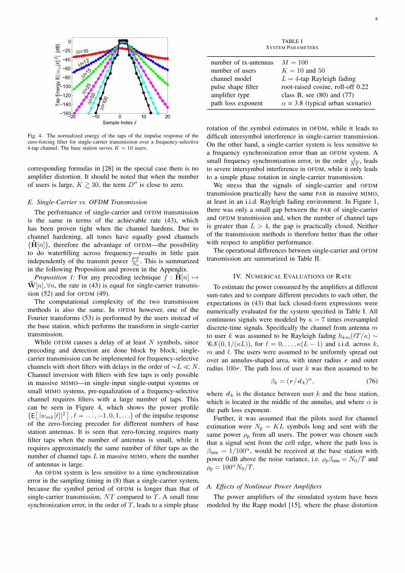
Fig. 4. The normalized energy of the taps of the impulse response of thezero-forcing filter for single-carrier transmission over a frequency-selective4-tap channel. The base station serves K = 10 users.

corresponding formulas in [28] in the special case there is noamplifier distortion. It should be noted that when the numberof users is large, K & 30, the term D′′ is close to zero.

E. Single-Carrier vs. OFDM Transmission

The performance of single-carrier and OFDM transmissionis the same in terms of the achievable rate (43), whichhas been proven tight when the channel hardens. Due tochannel hardening, all tones have equally good channels{H[n]}, therefore the advantage of OFDM—the possibilityto do waterfilling across frequency—results in little gainindependently of the transmit power PT

N0. This is summarized

in the following Proposition and proven in the Appendix.Proposition 1: For any precoding technique f : ˆH[n] 7→

W[n],∀n, the rate in (43) is equal for single-carrier transmis-sion (52) and for OFDM (49).

The computational complexity of the two transmissionmethods is also the same. In OFDM however, one of theFourier transforms (53) is performed by the users instead ofthe base station, which performs the transform in single-carriertransmission.

While OFDM causes a delay of at least N symbols, sinceprecoding and detection are done block by block, single-carrier transmission can be implemented for frequency-selectivechannels with short filters with delays in the order of ∼L � N .Channel inversion with filters with few taps is only possiblein massive MIMO—in single-input single-output systems orsmall MIMO systems, pre-equalization of a frequency-selectivechannel requires filters with a large number of taps. Thiscan be seen in Figure 4, which shows the power profile{E

[|wmk[`]|2

], ` = . . . ,−1, 0, 1, . . .} of the impulse response

of the zero-forcing precoder for different numbers of basestation antennas. It is seen that zero-forcing requires manyfilter taps when the number of antennas is small, while itrequires approximately the same number of filter taps as thenumber of channel taps L in massive MIMO, where the numberof antennas is large.

An OFDM system is less sensitive to a time synchronizationerror in the sampling timing in (8) than a single-carrier system,because the symbol period of OFDM is longer than that ofsingle-carrier transmission, NT compared to T . A small timesynchronization error, in the order of T , leads to a simple phase

TABLE ISYSTEM PARAMETERS

number of tx-antennas M = 100number of users K = 10 and 50channel model L = 4-tap Rayleigh fadingpulse shape filter root-raised cosine, roll-off 0.22amplifier type class B, see (80) and (77)path loss exponent α = 3.8 (typical urban scenario)

rotation of the symbol estimates in OFDM, while it leads todifficult intersymbol interference in single-carrier transmission.On the other hand, a single-carrier system is less sensitive toa frequency synchronization error than an OFDM system. Asmall frequency synchronization error, in the order 1

NT , leadsto severe intersymbol interference in OFDM, while it only leadsto a simple phase rotation in single-carrier transmission.

We stress that the signals of single-carrier and OFDMtransmission practically have the same PAR in massive MIMO,at least in an i.i.d. Rayleigh fading environment. In Figure 1,there was only a small gap between the PAR of single-carrierand OFDM transmission and, when the number of channel tapsis greater than L > 4, the gap is practically closed. Neitherof the transmission methods is therefore better than the otherwith respect to amplifier performance.

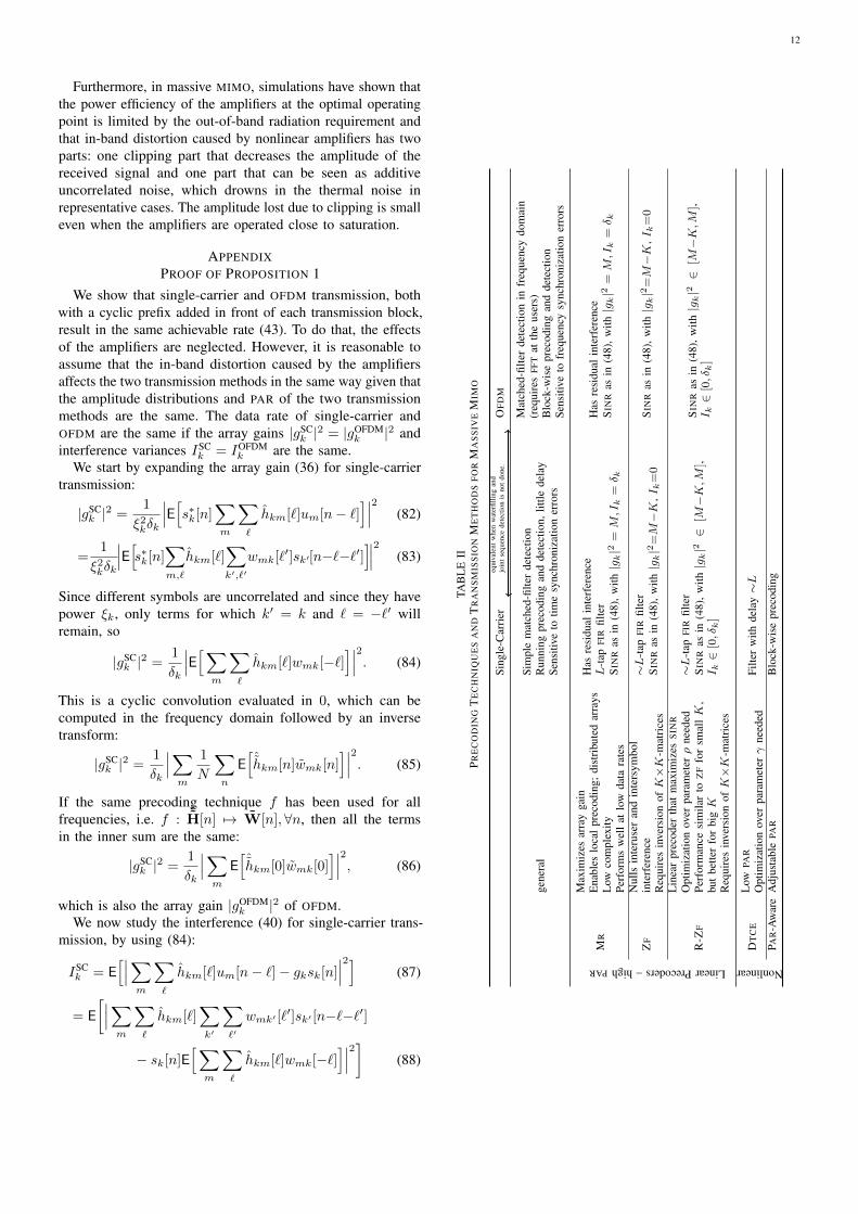
The operational differences between single-carrier and OFDMtransmission are summarized in Table II.

IV. NUMERICAL EVALUATIONS OF RATE

To estimate the power consumed by the amplifiers at differentsum-rates and to compare different precoders to each other, theexpectations in (43) that lack closed-form expressions werenumerically evaluated for the system specified in Table I. Allcontinuous signals were modeled by κ = 7 times oversampleddiscrete-time signals. Specifically the channel from antenna mto user k was assumed to be Rayleigh fading hkm(`T/κ) ∼CN(0, 1/(κL)), for ` = 0, . . . , κ(L − 1) and i.i.d. across k,m and `. The users were assumed to be uniformly spread outover an annulus-shaped area, with inner radius r and outerradius 100r. The path loss of user k was then assumed to be

βk = (r/dk)α, (76)

where dk is the distance between user k and the base station,which is located in the middle of the annulus, and where α isthe path loss exponent.

Further, it was assumed that the pilots used for channelestimation were Np = KL symbols long and sent with thesame power ρp from all users. The power was chosen suchthat a signal sent from the cell edge, where the path loss isβmin = 1/100α, would be received at the base station withpower 0 dB above the noise variance, i.e. ρpβmin = N0/T andρp = 100αN0/T .

A. Effects of Nonlinear Power Amplifiers

The power amplifiers of the simulated system have beenmodeled by the Rapp model [15], where the phase distortion

9

Power1Efficiency1η [a]0 20 40 60 80

Clip

ping

1Pow

er-

Loss

1ck1

[dB

]

-0.4

-0.3

-0.2

-0.1

0

201dB 141dB 101dB

5.21dB

2.21dB

0.21dB

-1.81dB

DTCE1PrecodingMaximum-Ratio1PrecodingZero-Forcing1Precoding

(a) The fraction of power lost due to clipping

Power5Efficiency5η [%]0 20 40 60 80

PA

5In-B

and5

Dis

tort

ion5

Dk

[dB

]

-80

-60

-40

-20

205dB

175dB

145dB

105dB

75dB5.25dB

35dB05dB

-1.8dB

(b) The variance of the received in-band distortion

Power1Efficiency1η [%]0 20 40 60 80

AC

LR1[d

B]

-90

-80

-70

-60

-50

-40

-30

-20

-10

201dB

141dB

101dB

5.21dB

2.21dB-1.81dB

(c) The amount of out-of-band radiation

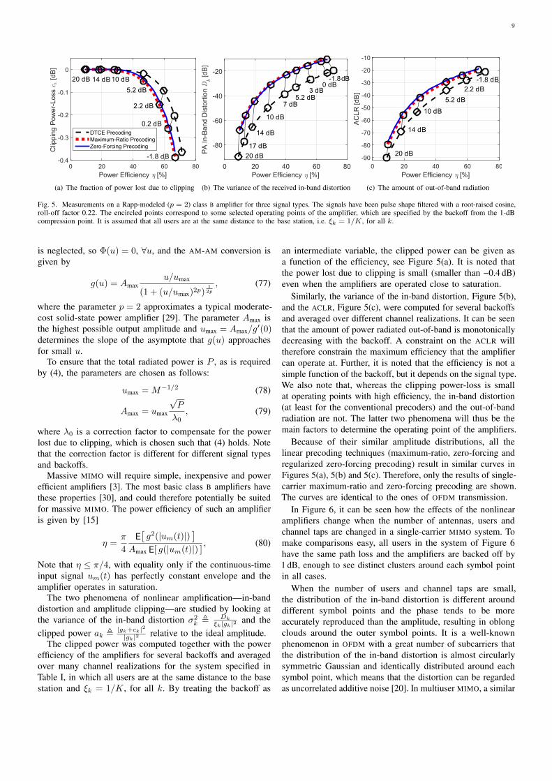
Fig. 5. Measurements on a Rapp-modeled (p = 2) class B amplifier for three signal types. The signals have been pulse shape filtered with a root-raised cosine,roll-off factor 0.22. The encircled points correspond to some selected operating points of the amplifier, which are specified by the backoff from the 1-dBcompression point. It is assumed that all users are at the same distance to the base station, i.e. ξk = 1/K, for all k.

is neglected, so Φ(u) = 0, ∀u, and the AM-AM conversion isgiven by

g(u) = Amaxu/umax

(1 + (u/umax)2p)12p

, (77)

where the parameter p = 2 approximates a typical moderate-cost solid-state power amplifier [29]. The parameter Amax isthe highest possible output amplitude and umax = Amax/g

′(0)determines the slope of the asymptote that g(u) approachesfor small u.

To ensure that the total radiated power is P , as is requiredby (4), the parameters are chosen as follows:

umax = M−1/2 (78)

Amax = umax

√P

λ0, (79)

where λ0 is a correction factor to compensate for the powerlost due to clipping, which is chosen such that (4) holds. Notethat the correction factor is different for different signal typesand backoffs.

Massive MIMO will require simple, inexpensive and powerefficient amplifiers [3]. The most basic class B amplifiers havethese properties [30], and could therefore potentially be suitedfor massive MIMO. The power efficiency of such an amplifieris given by [15]

η =π

4

E[g2(|um(t)|)

]Amax E[ g(|um(t)|) ]

, (80)

Note that η ≤ π/4, with equality only if the continuous-timeinput signal um(t) has perfectly constant envelope and theamplifier operates in saturation.

The two phenomena of nonlinear amplification—in-banddistortion and amplitude clipping—are studied by looking atthe variance of the in-band distortion σ2

k , Dk

ξk|gk|2 and theclipped power ak , |gk+ck|2

|gk|2 relative to the ideal amplitude.The clipped power was computed together with the power

efficiency of the amplifiers for several backoffs and averagedover many channel realizations for the system specified inTable I, in which all users are at the same distance to the basestation and ξk = 1/K, for all k. By treating the backoff as

an intermediate variable, the clipped power can be given asa function of the efficiency, see Figure 5(a). It is noted thatthe power lost due to clipping is small (smaller than −0.4 dB)even when the amplifiers are operated close to saturation.

Similarly, the variance of the in-band distortion, Figure 5(b),and the ACLR, Figure 5(c), were computed for several backoffsand averaged over different channel realizations. It can be seenthat the amount of power radiated out-of-band is monotonicallydecreasing with the backoff. A constraint on the ACLR willtherefore constrain the maximum efficiency that the amplifiercan operate at. Further, it is noted that the efficiency is not asimple function of the backoff, but it depends on the signal type.We also note that, whereas the clipping power-loss is smallat operating points with high efficiency, the in-band distortion(at least for the conventional precoders) and the out-of-bandradiation are not. The latter two phenomena will thus be themain factors to determine the operating point of the amplifiers.

Because of their similar amplitude distributions, all thelinear precoding techniques (maximum-ratio, zero-forcing andregularized zero-forcing precoding) result in similar curves inFigures 5(a), 5(b) and 5(c). Therefore, only the results of single-carrier maximum-ratio and zero-forcing precoding are shown.The curves are identical to the ones of OFDM transmission.

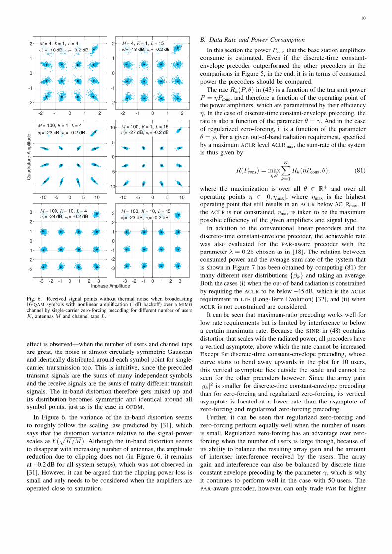
In Figure 6, it can be seen how the effects of the nonlinearamplifiers change when the number of antennas, users andchannel taps are changed in a single-carrier MIMO system. Tomake comparisons easy, all users in the system of Figure 6have the same path loss and the amplifiers are backed off by1 dB, enough to see distinct clusters around each symbol pointin all cases.

When the number of users and channel taps are small,the distribution of the in-band distortion is different arounddifferent symbol points and the phase tends to be moreaccurately reproduced than the amplitude, resulting in oblongclouds around the outer symbol points. It is a well-knownphenomenon in OFDM with a great number of subcarriers thatthe distribution of the in-band distortion is almost circularlysymmetric Gaussian and identically distributed around eachsymbol point, which means that the distortion can be regardedas uncorrelated additive noise [20]. In multiuser MIMO, a similar

10

-2 -1 0 1 2

-2

-1

0

1

2 M = 4, K = 1, L = 4σ 2 = -18 dB, a = -0.2 dB

-2 -1 0 1 2

-2

-1

0

1

2 M = 4, K = 1, L = 15σ 2= -18 dB, a = -0.2 dB

-10 -5 0 5 10

Qua

drat

ure

Ampl

itude

M = 100, K = 1, L = 4σ2= -23 dB, a = -0.2 dB

-10 -5 0 5 10

-10

-5

0

5

10 M = 100, K = 1, L = 15σ2= -27 dB, a = -0.2 dB

-3 -2 -1 0 1 2 3

-3

-2

-1

0

1

2

3 M = 100, K = 10, L = 4σ 2= -24 dB, a = -0.2 dB

Inphase Amplitude-2 0 2

-3

-2

-1

0

1

2

3

-3 -1 1 3

M = 100, K = 10, L = 15σ2= -23 dB, a = -0.2 dB

k k kk

k k k k

k k k k

Fig. 6. Received signal points without thermal noise when broadcasting16-QAM symbols with nonlinear amplification (1 dB backoff) over a MIMOchannel by single-carrier zero-forcing precoding for different number of usersK, antennas M and channel taps L.

effect is observed—when the number of users and channel tapsare great, the noise is almost circularly symmetric Gaussianand identically distributed around each symbol point for single-carrier transmission too. This is intuitive, since the precodedtransmit signals are the sums of many independent symbolsand the receive signals are the sums of many different transmitsignals. The in-band distortion therefore gets mixed up andits distribution becomes symmetric and identical around allsymbol points, just as is the case in OFDM.

In Figure 6, the variance of the in-band distortion seemsto roughly follow the scaling law predicted by [31], whichsays that the distortion variance relative to the signal powerscales as O(

√K/M). Although the in-band distortion seems

to disappear with increasing number of antennas, the amplitudereduction due to clipping does not (in Figure 6, it remainsat −0.2 dB for all system setups), which was not observed in[31]. However, it can be argued that the clipping power-loss issmall and only needs to be considered when the amplifiers areoperated close to saturation.

B. Data Rate and Power Consumption

In this section the power Pcons that the base station amplifiersconsume is estimated. Even if the discrete-time constant-envelope precoder outperformed the other precoders in thecomparisons in Figure 5, in the end, it is in terms of consumedpower the precoders should be compared.

The rate Rk(P, θ) in (43) is a function of the transmit powerP = ηPcons, and therefore a function of the operating point ofthe power amplifiers, which are parametrized by their efficiencyη. In the case of discrete-time constant-envelope precoding, therate is also a function of the parameter θ = γ. And in the caseof regularized zero-forcing, it is a function of the parameterθ = ρ. For a given out-of-band radiation requirement, specifiedby a maximum ACLR level ACLRmax, the sum-rate of the systemis thus given by

R(Pcons) = maxη,θ

K∑k=1

Rk(ηPcons, θ), (81)

where the maximization is over all θ ∈ R+ and over alloperating points η ∈ [0, ηmax], where ηmax is the highestoperating point that still results in an ACLR below ACLRmax. Ifthe ACLR is not constrained, ηmax is taken to be the maximumpossible efficiency of the given amplifiers and signal type.

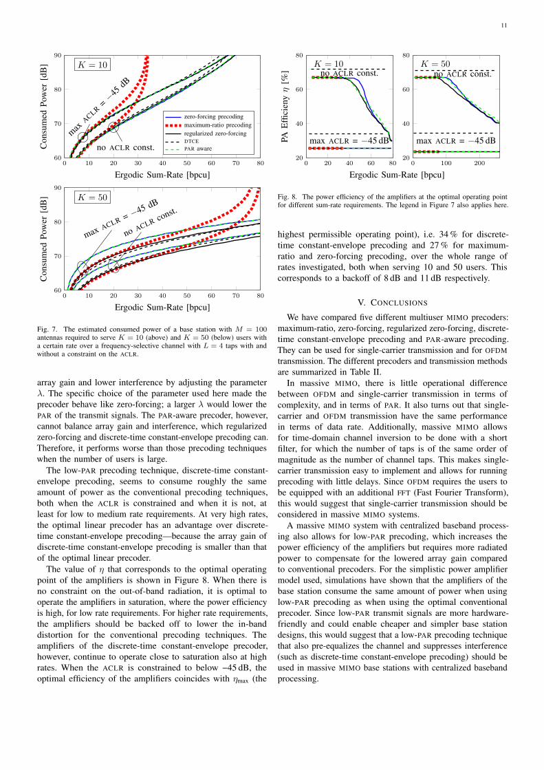
In addition to the conventional linear precoders and thediscrete-time constant-envelope precoder, the achievable ratewas also evaluated for the PAR-aware precoder with theparameter λ = 0.25 chosen as in [18]. The relation betweenconsumed power and the average sum-rate of the system thatis shown in Figure 7 has been obtained by computing (81) formany different user distributions {βk} and taking an average.Both the cases (i) when the out-of-band radiation is constrainedby requiring the ACLR to be below −45 dB, which is the ACLRrequirement in LTE (Long-Term Evolution) [32], and (ii) whenACLR is not constrained are considered.

It can be seen that maximum-ratio precoding works well forlow rate requirements but is limited by interference to belowa certain maximum rate. Because the SINR in (48) containsdistortion that scales with the radiated power, all precoders havea vertical asymptote, above which the rate cannot be increased.Except for discrete-time constant-envelope precoding, whosecurve starts to bend away upwards in the plot for 10 users,this vertical asymptote lies outside the scale and cannot beseen for the other precoders however. Since the array gain|gk|2 is smaller for discrete-time constant-envelope precodingthan for zero-forcing and regularized zero-forcing, its verticalasymptote is located at a lower rate than the asymptote ofzero-forcing and regularized zero-forcing precoding.

Further, it can be seen that regularized zero-forcing andzero-forcing perform equally well when the number of usersis small. Regularized zero-forcing has an advantage over zero-forcing when the number of users is large though, because ofits ability to balance the resulting array gain and the amountof interuser interference received by the users. The arraygain and interference can also be balanced by discrete-timeconstant-envelope precoding by the parameter γ, which is whyit continues to perform well in the case with 50 users. ThePAR-aware precoder, however, can only trade PAR for higher

11

0 10 20 30 40 50 60 70 8060

70

80

90

no ACLR const.

maxACLR

=−45

dB

K = 10

Ergodic Sum-Rate [bpcu]

Con

sum

edPo

wer

[dB

]

zero-forcing precodingmaximum-ratio precodingregularized zero-forcingDTCEPAR aware

0 10 20 30 40 50 60 70 8060

70

80

90

no ACLR const.

max ACLR = −45 dBK = 50

Ergodic Sum-Rate [bpcu]

Con

sum

edPo

wer

[dB

]

Fig. 7. The estimated consumed power of a base station with M = 100antennas required to serve K = 10 (above) and K = 50 (below) users witha certain rate over a frequency-selective channel with L = 4 taps with andwithout a constraint on the ACLR.

array gain and lower interference by adjusting the parameterλ. The specific choice of the parameter used here made theprecoder behave like zero-forcing; a larger λ would lower thePAR of the transmit signals. The PAR-aware precoder, however,cannot balance array gain and interference, which regularizedzero-forcing and discrete-time constant-envelope precoding can.Therefore, it performs worse than those precoding techniqueswhen the number of users is large.

The low-PAR precoding technique, discrete-time constant-envelope precoding, seems to consume roughly the sameamount of power as the conventional precoding techniques,both when the ACLR is constrained and when it is not, atleast for low to medium rate requirements. At very high rates,the optimal linear precoder has an advantage over discrete-time constant-envelope precoding—because the array gain ofdiscrete-time constant-envelope precoding is smaller than thatof the optimal linear precoder.

The value of η that corresponds to the optimal operatingpoint of the amplifiers is shown in Figure 8. When there isno constraint on the out-of-band radiation, it is optimal tooperate the amplifiers in saturation, where the power efficiencyis high, for low rate requirements. For higher rate requirements,the amplifiers should be backed off to lower the in-banddistortion for the conventional precoding techniques. Theamplifiers of the discrete-time constant-envelope precoder,however, continue to operate close to saturation also at highrates. When the ACLR is constrained to below −45 dB, theoptimal efficiency of the amplifiers coincides with ηmax (the

0 20 40 60 8020

40

60

80

no ACLR const.

max ACLR = −45 dB

K = 10

Ergodic Sum-Rate [bpcu]

PAE

ffici

enyη

[%]

0 100 20020

40

60

80

no ACLR const.

max ACLR = −45 dB

K = 50

Fig. 8. The power efficiency of the amplifiers at the optimal operating pointfor different sum-rate requirements. The legend in Figure 7 also applies here.

highest permissible operating point), i.e. 34 % for discrete-time constant-envelope precoding and 27 % for maximum-ratio and zero-forcing precoding, over the whole range ofrates investigated, both when serving 10 and 50 users. Thiscorresponds to a backoff of 8 dB and 11 dB respectively.

V. CONCLUSIONS

We have compared five different multiuser MIMO precoders:maximum-ratio, zero-forcing, regularized zero-forcing, discrete-time constant-envelope precoding and PAR-aware precoding.They can be used for single-carrier transmission and for OFDMtransmission. The different precoders and transmission methodsare summarized in Table II.

In massive MIMO, there is little operational differencebetween OFDM and single-carrier transmission in terms ofcomplexity, and in terms of PAR. It also turns out that single-carrier and OFDM transmission have the same performancein terms of data rate. Additionally, massive MIMO allowsfor time-domain channel inversion to be done with a shortfilter, for which the number of taps is of the same order ofmagnitude as the number of channel taps. This makes single-carrier transmission easy to implement and allows for runningprecoding with little delays. Since OFDM requires the users tobe equipped with an additional FFT (Fast Fourier Transform),this would suggest that single-carrier transmission should beconsidered in massive MIMO systems.

A massive MIMO system with centralized baseband process-ing also allows for low-PAR precoding, which increases thepower efficiency of the amplifiers but requires more radiatedpower to compensate for the lowered array gain comparedto conventional precoders. For the simplistic power amplifiermodel used, simulations have shown that the amplifiers of thebase station consume the same amount of power when usinglow-PAR precoding as when using the optimal conventionalprecoder. Since low-PAR transmit signals are more hardware-friendly and could enable cheaper and simpler base stationdesigns, this would suggest that a low-PAR precoding techniquethat also pre-equalizes the channel and suppresses interference(such as discrete-time constant-envelope precoding) should beused in massive MIMO base stations with centralized basebandprocessing.

12

Furthermore, in massive MIMO, simulations have shown thatthe power efficiency of the amplifiers at the optimal operatingpoint is limited by the out-of-band radiation requirement andthat in-band distortion caused by nonlinear amplifiers has twoparts: one clipping part that decreases the amplitude of thereceived signal and one part that can be seen as additiveuncorrelated noise, which drowns in the thermal noise inrepresentative cases. The amplitude lost due to clipping is smalleven when the amplifiers are operated close to saturation.

APPENDIXPROOF OF PROPOSITION 1

We show that single-carrier and OFDM transmission, bothwith a cyclic prefix added in front of each transmission block,result in the same achievable rate (43). To do that, the effectsof the amplifiers are neglected. However, it is reasonable toassume that the in-band distortion caused by the amplifiersaffects the two transmission methods in the same way given thatthe amplitude distributions and PAR of the two transmissionmethods are the same. The data rate of single-carrier andOFDM are the same if the array gains |gSC

k |2 = |gOFDMk |2 and

interference variances ISCk = IOFDM

k are the same.We start by expanding the array gain (36) for single-carrier

transmission:

|gSCk |2 =

1

ξ2kδk

∣∣∣E[s∗k[n]∑m

∑`

hkm[`]um[n− `]]∣∣∣2 (82)

=1

ξ2kδk

∣∣∣E[s∗k[n]∑m,`

hkm[`]∑k′,`′

wmk[`′]sk′[n−`−`′]

]∣∣∣2 (83)

Since different symbols are uncorrelated and since they havepower ξk, only terms for which k′ = k and ` = −`′ willremain, so

|gSCk |2 =

1

δk

∣∣∣E[∑m

∑`

hkm[`]wmk[−`]]∣∣∣2. (84)

This is a cyclic convolution evaluated in 0, which can becomputed in the frequency domain followed by an inversetransform:

|gSCk |2 =

1

δk

∣∣∣∑m

1

N

∑n

E[ˆhkm[n]wmk[n]

]∣∣∣2. (85)

If the same precoding technique f has been used for allfrequencies, i.e. f : ˆH[n] 7→ W[n],∀n, then all the termsin the inner sum are the same:

|gSCk |2 =

1

δk

∣∣∣∑m

E[ˆhkm[0]wmk[0]

]∣∣∣2, (86)

which is also the array gain |gOFDMk |2 of OFDM.

We now study the interference (40) for single-carrier trans-mission, by using (84):

ISCk = E

[∣∣∣∑m

∑`

hkm[`]um[n− `]− gksk[n]∣∣∣2] (87)

= E

[∣∣∣∑m

∑`

hkm[`]∑k′

∑`′

wmk′ [`′]sk′ [n−`−`′]

− sk[n]E[∑

m

∑`

hkm[`]wmk[−`]]∣∣∣2] (88)

TAB

LE

IIP

RE

CO

DIN

GT

EC

HN

IQU

ES

AN

DT

RA

NS

MIS

SIO

NM

ET

HO

DS

FO

RM

AS

SIV

EM

IMO

Sing

le-C

arri

erO

FD

M

gene

ral

Sim

ple

mat

ched

-filte

rde

tect

ion

Run

ning

prec

odin

gan

dde

tect

ion,

little

dela

ySe

nsiti

veto

time

sync

hron

izat

ion

erro

rs

Mat

ched

-filte

rde

tect

ion

infr

eque

ncy

dom

ain

(req

uire

sFF

Tat

the

user

s)B

lock

-wis

epr

ecod

ing

and

dete

ctio

nSe

nsiti

veto

freq

uenc

ysy

nchr

oniz

atio

ner

rors

LinearPrecoders–highPAR

MR

Max

imiz

esar

ray

gain

Ena

bles

loca

lpr

ecod

ing;

dist

ribu

ted

arra

ysL

owco

mpl

exity

Perf

orm

sw

ell

atlo

wda

tara

tes

Has

resi

dual

inte

rfer

ence

L-t

apFI

Rfil

ter

SIN

Ras

in(4

8),w

ith|g

k|2

=M

,Ik=

δ k

Has

resi

dual

inte

rfer

ence

SIN

Ras

in(4

8),w

ith|g

k|2

=M

,Ik=

δ k

ZF

Nul

lsin

teru

ser

and

inte

rsym

bol

inte

rfer

ence

Req

uire

sin

vers

ion

ofK×K

-mat

rice

s

∼L

-tap

FIR

filte

rS

INR

asin

(48)

,with

|gk|2=M

−K

,Ik=0

SIN

Ras

in(4

8),w

ith|g

k|2=M

−K

,Ik=0

R-Z

F

Lin

ear

prec

oder

that

max

imiz

esS

INR

Opt

imiz

atio

nov

erpa

ram

eter

ρne

eded

Perf

orm

ance

sim

ilar

toZ

Ffo

rsm

allK

,bu

tbe

tter

for

bigK

Req

uire

sin

vers

ion

ofK×K

-mat

rice

s

∼L

-tap

FIR

filte

rS

INR

asin

(48)

,w

ith|g

k|2

∈[M

−K,M

],I k

∈[0,δ

k]

SIN

Ras

in(4

8),

with

|gk|2

∈[M

−K,M

],I k

∈[0,δ

k]

Nonlinear

DT

CE

Low

PAR

Opt

imiz

atio

nov

erpa

ram

eter

γne

eded

Filte

rw

ithde

lay∼L

PAR

-Aw

are

Adj

usta

ble

PAR

Blo

ck-w

ise

prec

odin

gequi

vale

ntw

hen

wat

erfil

ling

and

join

tse

quen

cede

tect

ion

isno

tdo

ne.

13

= E

[∣∣∣sk[n](∑m,`

hkm[`]wmk[−`]−E[∑m,`

hkm[`]wmk[−`]])

+∑∑

(k′,n′)6=(k,0)

sk′ [n′]∑m

∑`

hkm[`]wmk′ [n′ − `]∣∣∣2] (89)

Since different symbols are uncorrelated and since they havepower ξk, the square is expanded into the following.

ISCk =

∑k′

∑n′

ξk′E[∣∣∣∑

m

∑`

hkm[`]wmk′ [n′ − `]∣∣∣2]

− ξk

∣∣∣E[∑m

∑`

hkm[`]wmk[−`]]∣∣∣2 (90)

The two terms are cyclic convolutions in n′ and 0 respectivelyand can be computed in the frequency domain. Along the sameline of reasoning as in (86), the interference variance is givenby ISC

k =∑k′

ξk′E[∣∣∑

m

ˆhkm[0]wmk′ [0]

∣∣2]−ξk

∣∣∣E[∑m

ˆhkm[0]wmk[0]

]∣∣∣2,(91)

which is precisely the interference variance IOFDMk of OFDM

at tone 0, or at any other tone.That the rate (43) is the same for single-carrier and OFDM

transmission was proven, in a different way, for the specialcase maximum-ratio precoding in [24].

REFERENCES

[1] C. Mollen, E. G. Larsson, and T. Eriksson, “On the impact of PA-inducedin-band distortion in massive MIMO,” The Proceedings of the EuropeanWireless Conference, May 2014.

[2] T. L. Marzetta, “Noncooperative cellular wireless with unlimited numbersof base station antennas,” IEEE Transactions on Wireless Communica-tions, vol. 9, no. 11, pp. 3590–3600, Oct. 2010.

[3] E. G. Larsson, O. Edfors, F. Tufvesson, and T. L. Marzetta, “MassiveMIMO for next generation wireless systems,” IEEE CommunicationsMagazine, vol. 52, no. 2, pp. 186–195, Feb. 2014.

[4] H. Q. Ngo, E. G. Larsson, and T. L. Marzetta, “Energy and spectralefficiency of very large multiuser MIMO systems,” IEEE Transactionson Communications, vol. 61, no. 4, pp. 1436–1449, Feb. 2013.

[5] H. Yang and T. L. Marzetta, “Performance of conjugate and zero-forcingbeamforming in large-scale antenna systems,” IEEE Journal on SelectedAreas in Communications, vol. 31, no. 2, pp. 172–179, Feb. 2013.

[6] J. Hoydis, K. Hosseini, S. t. Brink, and M. Debbah, “Making smart useof excess antennas: Massive MIMO, small cells, and TDD,” Bell LabsTechnical Journal, vol. 18, no. 2, pp. 5–21, Sep. 2013.

[7] G. Caire and S. Shamai, “On the achievable throughput of a multiantennaGaussian broadcast channel,” IEEE Transactions on Information Theory,vol. 49, no. 7, pp. 1691–1706, Jul. 2003.

[8] A. Goldsmith, S. A. Jafar, N. Jindal, and S. Vishwanath, “Capacity limitsof MIMO channels,” IEEE Journal on Selected Areas in Communications,vol. 21, no. 5, pp. 684–702, Jun. 2003.

[9] M. Joham, W. Utschick, and J. A. Nossek, “Linear transmit processingin MIMO communications systems,” IEEE Transactions on SignalProcessing, vol. 53, no. 8, pp. 2700–2712, Aug. 2005.

[10] E. Bjornson, M. Bengtsson, and B. Ottersten, “Optimal multiuser transmitbeamforming: A difficult problem with a simple solution structure,” IEEESignal Processing Magazine, vol. 31, no. 4, pp. 142–148, Jul. 2014.

[11] M. Vu, “MISO capacity with per-antenna power constraint,” IEEETransactions on Communications, vol. 59, no. 5, pp. 1268–1274, Mar.2011.

[12] ——, “MIMO capacity with per-antenna power constraint,” in Proc.IEEE Global Telecommunications Conference, Dec. 2011, pp. 1–5.

[13] W. Yu and T. Lan, “Transmitter optimization for the multi-antennadownlink with per-antenna power constraints,” IEEE Transactions onSignal Processing, vol. 55, no. 6, pp. 2646–2660, Jun. 2007.

[14] H. Hemesi, A. Abdipour, and A. Mohammadi, “Analytical modeling ofMIMO-OFDM system in the presence of nonlinear power amplifier withmemory,” IEEE Transactions on Communications, vol. 61, no. 1, pp.155–163, Nov. 2013.

[15] H. Ochiai, “An analysis of band-limited communication systems fromamplifier efficiency and distortion perspective,” IEEE Transactions onCommunications, vol. 61, no. 4, pp. 1460–1472, Feb. 2013.

[16] S. Mohammed and E. G. Larsson, “Constant-envelope multi-user pre-coding for frequency-selective massive MIMO systems,” IEEE WirelessCommunications Letters, vol. 2, no. 5, pp. 547–550, Oct. 2013.

[17] ——, “Per-antenna constant envelope precoding for large multi-userMIMO systems,” IEEE Transactions on Communications, vol. 61, no. 3,pp. 1059–1071, Mar. 2013.

[18] C. Studer and E. G. Larsson, “PAR-aware large-scale multi-user MIMO-OFDM downlink,” IEEE Journal on Selected Areas in Communications,vol. 31, no. 2, pp. 303–313, Feb. 2013.

[19] E. Bjornson, J. Hoydis, M. Kountouris, and M. Debbah, “Massive MIMOsystems with non-ideal hardware: Energy efficiency, estimation, andcapacity limits,” IEEE Transactions on Information Theory, vol. 60,no. 11, pp. 7112–7139, Nov. 2014.

[20] E. Costa, M. Midrio, and S. Pupolin, “Impact of amplifier nonlinearitieson OFDM transmission system performance,” IEEE CommunicationsLetters, vol. 3, no. 2, pp. 37–39, Feb. 1999.

[21] J. Qi and S. Aıssa, “Analysis and compensation of power amplifiernonlinearity in MIMO transmit diversity systems,” IEEE Transactionson Vehicular Technology, vol. 59, no. 6, pp. 2921–2931, May 2010.

[22] M. Medard, “The effect upon channel capacity in wireless commu-nications of perfect and imperfect knowledge of the channel,” IEEETransactions on Information Theory, vol. 46, no. 3, pp. 933–946, May2000.

[23] B. Hassibi and B. M. Hochwald, “How much training is needed inmultiple-antenna wireless links?” IEEE Transactions on InformationTheory, vol. 49, no. 4, pp. 951–963, Apr. 2003.

[24] A. Pitarokoilis, S. K. Mohammed, and E. G. Larsson, “On the optimalityof single-carrier transmission in large-scale antenna systems,” IEEEWireless Communications Letters, vol. 1, no. 4, pp. 276–279, Apr. 2012.

[25] A. M. Tulino and S. Verdu, Random Matrix Theory and WirelessCommunications. Now Publishers Inc., 2004, vol. 1.

[26] L. Sanguinetti, E. Bjornson, M. Debbah, and A. L. Moustakas, “Optimallinear precoding in multi-user MIMO systems: A large system analysis,”in The Proceedings of the IEEE Global Communications Conference,Dec. 2014, pp. 3922–3927.

[27] S. Mohammed and E. G. Larsson, “Single-user beamforming in large-scale MISO systems with per-antenna constant-envelope constraints: Thedoughnut channel,” IEEE Transactions on Wireless Communications,vol. 11, no. 11, pp. 3992–4005, Sep. 2012.

[28] H. Yang and T. L. Marzetta, “A macro cellular wireless network withuniformly high user throughputs,” in The Proceedings of the VehicularTechnology Conference, Sep. 2014, pp. 1–5.

[29] N. Benvenuto, R. Dinis, D. Falconer, and S. Tomasin, “Single carriermodulation with nonlinear frequency domain equalization: An idea whosetime has come—again,” Proceedings of the IEEE, vol. 98, no. 1, pp.69–96, 2010.

[30] F. H. Raab, P. Asbeck, S. Cripps, P. B. Kenington, Z. B. Popovic,N. Pothecary, J. F. Sevic, and N. O. Sokal, “Power amplifiers andtransmitters for RF and microwave,” IEEE Transactions on MicrowaveTheory and Techniques, vol. 50, no. 3, pp. 814–826, Mar. 2002.

[31] E. Bjornson, M. Matthaiou, and M. Debbah, “Massive MIMO witharbitrary non-ideal arrays: Hardware scaling laws and circuit-awaredesign,” ArXiv E-Print, Sep. 2014, arXiv:1409.0875 [cs.IT].

[32] 3GPP TS36.141 3rd Generation Partnership Project; Technical Specifica-tion Group Radio Access Network; Evolved Universal Terrestrial RadioAccess (E-UTRA); Base Station (BS) Conformance Testing (Release 10),3GPP Std., Rev. V10.2.0, 2011.

14

Christopher Mollen received his M.Sc. degree fromLinkoping University, Sweden, in 2013, where heis currently pursuing his the Ph.D. degree with theDepartment of Electrical Engineering, Division forCommunication Systems. His research interest is low-complexity hardware implementations of massiveMIMO base stations, including low-PAR precoding,one-bit ADCs, and nonlinear amplifiers. Prior to hisPh.D. studies, he worked as an Intern at Ericsson inKista, Sweden, and in Shanghai, China. From 2015to 2016, he visited the University of Texas at Austin

as a Fulbright Scholar.

Erik G. Larsson received his Ph.D. degree fromUppsala University, Sweden, in 2002. Since 2007,he is Professor in the Department of ElectricalEngineering (ISY) at Linkoping University (LiU)in Linkoping, Sweden. He has previously beenAssociate Professor (Docent) at the Royal Instituteof Technology (KTH) in Stockholm, Sweden, andan Assistant Professor with the University of Floridaand the George Washington University, USA. In thespring of 2015 he was a Visiting Fellow at PrincetonUniversity, USA, for four months.

His main professional interests are within the areas of wireless communi-cations and signal processing. He has authored some 120 journal papers onthese topics, co-authored the textbook entitled Space-Time Block Coding forWireless Communications (Cambridge Univ. Press, 2003) and holds 15 issuedand several pending patents on wireless technology.

He received the IEEE Signal Processing Magazine Best Column Awardtwice, in 2012 and 2014, and the IEEE ComSoc Stephen O. Rice Prizein Communications Theory in 2015. He served as Associate Editor forseveral major journals, including the IEEE Transactions on Communications(2010–2014) and IEEE Transactions on Signal Processing (2006–2010). Heserves as chair of the IEEE Signal Processing Society SPCOM technicalcommittee in 2015–2016 and he served as chair of the steering committee forthe IEEE Wireless Communications Letters from 2014 to 2015. He was theGeneral Chair of the Asilomar Conference on Signals, Systems and Computersin 2015, and Technical Chair in 2012. He is a Fellow of the IEEE.

Thomas Eriksson received the Ph.D. degree ininformation theory from Chalmers University ofTechnology, Gothenburg, Sweden, in 1996. From1990 to 1996, he was with Chalmers University ofTechnology. In 1997 and 1998, he was with AT&TLabs-Research, Murray Hill, NJ, USA. In 1998 and1999, he was with Ericsson Radio Systems AB, Kista,Sweden. Since 1999, he has been with ChalmersUniversity of Technology, where he is currently aProfessor of communication systems. Furthermore,he was a Guest Professor with Yonsei University,

South Korea, from 2003 to 2004. He has authored or co-authored over 200journal and conference papers, and holds eight patents.

He is leading the research efforts on hardware-constrained communicationswith Chalmers University of Technology.

His research interests include communication, data compression, andmodeling and compensation of nonideal hardware components (e.g., amplifiers,oscillators, and modulators in communication transmitters and receivers,including massive MIMO). He is currently the Vice Head of the Departmentof Signals and Systems with the Chalmers University of Technology, wherehe is responsible for undergraduate and master’s education.