watershed modeling system - university of texas at …1 introduction chapter 1 introduction this...
TRANSCRIPT

Watershed Modeling System
WMS v7.0
TUTORIALS


WMS 7.0 Tutorials
Copyright © 2002 Brigham Young University - Environmental Modeling Research Laboratory
All Rights Reserved
Unauthorized duplication of the WMS software or documentation is strictly prohibited.
THE BRIGHAM YOUNG UNIVERSITY ENVIRONMENTAL MODELING RESEARCH LABORATORY MAKES NO WARRANTIES EITHER EXPRESS OR IMPLIED REGARDING THE PROGRAM WMS AND ITS FITNESS FOR ANY PARTICULAR PURPOSE OR THE VALIDITY OF THE INFORMATION CONTAINED IN THIS USER'S MANUAL
The software WMS is a product of the Environmental Modeling Research Laboratory of Brigham Young University. For more information about this software and related products, contact the EMRL at:
Environmental Modeling Research Laboratory Rm. 242, Clyde Building Brigham Young University Provo, Utah 84602 Tel.: (801) 422-2812 e-mail: [email protected] WWW: http://www.emrl.byu.edu/wms.html
For technical support, contact your WMS reseller.

TABLE OF CONTENTS
1 INTRODUCTION....................................................................................................................................................... 1-1 1.1 SUGGESTED ORDER OF COMPLETION ...........................................................................................................1-1 1.2 TUTORIAL FILES................................................................................................................................................1-2 1.3 STARTING OVER................................................................................................................................................1-2 1.4 GETTING AROUND THE WMS INTERFACE ..................................................................................................1-2
2 IMAGES ....................................................................................................................................................................... 2-1 2.1 OBJECTIVES ........................................................................................................................................................2-1 2.2 GEOTIFF FILES ...................................................................................................................................................2-2 2.3 WORLD FILES.....................................................................................................................................................2-4 2.4 REGISTERING SCANNED IMAGES.....................................................................................................................2-4 2.5 AERIAL PHOTOGRAPHS....................................................................................................................................2-8 2.6 CONCLUSION ....................................................................................................................................................2-12
3 BASIC FEATURE OBJECTS .................................................................................................................................. 3-1 3.1 OBJECTIVES ........................................................................................................................................................3-1 3.2 CREATING AND EDITING FEATURE OBJECTS...............................................................................................3-2 3.3 USING SHAPE FILES TO CREATE FEATURE OBJECTS.................................................................................3-7 3.4 CREATING FEATURE OBJECTS USING BACKGROUND IMAGES...................................................................3-9 3.5 MORE FEATURE OBJECTS FROM IMAGES....................................................................................................3-12 3.6 DISPLAY OPTIONS...........................................................................................................................................3-13 3.7 CONCLUSION ....................................................................................................................................................3-14
4 ADVANCED FEATURE OBJECTS........................................................................................................................ 4-1 4.1 OBJECTIVES ........................................................................................................................................................4-1 4.2 CREATING A WATERSHED FROM SCRATCH WITH FEATURE OBJECTS...................................................4-2 4.3 CLEANING...........................................................................................................................................................4-5 4.4 FEATURE OBJECTS FROM CAD DATA.........................................................................................................4-13 4.5 CONCLUSIONS...................................................................................................................................................4-15
5 DEM BASICS ............................................................................................................................................................. 5-1 5.1 OBJECTIVES ........................................................................................................................................................5-1 5.2 GETTING DEMS FROM THE INTERNET .........................................................................................................5-2 5.3 MERGING DEMS.................................................................................................................................................5-7 5.4 TRIMMING DEMS...............................................................................................................................................5-8 5.5 DISPLAYING DEMS............................................................................................................................................5-9 5.6 CONCLUSION ....................................................................................................................................................5-11
6 DEM DELINEATION................................................................................................................................................. 6-1 6.1 OBJECTIVES ........................................................................................................................................................6-1 6.2 IMPORTING DEM DATA...................................................................................................................................6-2 6.3 COMPUTING FLOW DATA AND ACCUMULATIONS.....................................................................................6-3 6.4 DELINEATING WATERSHEDS FROM DEMS...................................................................................................6-4

vi WMS Tutorials
6.5 CREATING SUB-BASINS.....................................................................................................................................6-6 6.6 ADDING A STREAM ARC AND REDEFINING BASINS....................................................................................6-9 6.7 DISPLAYING DEMS..........................................................................................................................................6-13 6.8 CONCLUSIONS...................................................................................................................................................6-15
7 EDITING DEMS.......................................................................................................................................................... 7-1 7.1 OBJECTIVES ........................................................................................................................................................7-1 7.2 RUNNING TOPAZ AND BASIN DELINEATION ..............................................................................................7-2 7.3 DEM FILL COMMAND ......................................................................................................................................7-3 7.4 EDITING FLOW DIRECTIONS ...........................................................................................................................7-6 7.5 EDITING ELEVATIONS TO CREATE STREAMS............................................................................................7-11 7.6 EDITING ELEVATIONS USING FEATURE ARCS............................................................................................7-16 7.7 COMPUTING A STORAGE CAPACITY CURVE..............................................................................................7-19 7.8 HYDROGRAPH ROUTING ................................................................................................................................7-19
8 USING TRIANGULATED IRREGULAR NETWORKS....................................................................................... 8-1 8.1 OBJECTIVES ........................................................................................................................................................8-1 8.2 IMPORTING SURVEY DATA .............................................................................................................................8-2 8.3 DIGITIZING DATA .............................................................................................................................................8-2 8.4 TRIANGULATION ...............................................................................................................................................8-3 8.5 AUTOMATED TIN EDITING.............................................................................................................................8-3 8.6 MANUAL TIN EDITING.....................................................................................................................................8-6 8.7 CREATING A TIN USING A CONCEPTUAL MODEL ....................................................................................8-12 8.8 CONVERT TO DEM..........................................................................................................................................8-16 8.9 EXPORTING DATA TO CAD..........................................................................................................................8-18
9 HEC-1 INTERFACE................................................................................................................................................... 9-1 9.1 OBJECTIVES ........................................................................................................................................................9-1 9.2 DELINEATING THE WATERSHED ...................................................................................................................9-2 9.3 SINGLE BASIN ANALYSIS.................................................................................................................................9-7 9.4 COMPUTING THE CN USING LAND USE AND SOILS DATA ......................................................................9-11 9.5 ADDING SUB-BASINS AND ROUTING............................................................................................................9-13 9.6 MODELING A RESERVOIR IN HEC-1..............................................................................................................9-18 9.7 REVIEWING OUTPUT ......................................................................................................................................9-22 9.8 CONCLUSION ....................................................................................................................................................9-22
10 RATIONAL METHOD INTERFACE...............................................................................................................10-1 10.1 READING IN TERRAIN DATA.........................................................................................................................10-1 10.2 RUNNING A RATIONAL METHOD SIMULATION........................................................................................10-2 10.3 ADDING A DETENTION BASIN....................................................................................................................10-10 10.4 CONCLUSIONS.................................................................................................................................................10-11
11 NATIONAL FLOOD FREQUENCY PROGRAM (NFF) INTERFACE.......................................................11-1 11.1 OPENING THE DRAINAGE BASIN ..................................................................................................................11-1 11.2 PREPARE THE BASIN FOR USE WITH NFF...................................................................................................11-2 11.3 CALCULATING PERCENTAGE OF LAKE COVER..........................................................................................11-3 11.4 RUNNING NFF ..................................................................................................................................................11-6 11.5 UTILIZING AN NFF REGION COVERAGE ......................................................................................................11-8 11.6 CONCLUSIONS.................................................................................................................................................11-12
12 TIME OF CONCENTRATION CALCULATIONS AND COMPUTING A COMPOSITE CN..............12-1 12.1 READING A TIN FILE ......................................................................................................................................12-2

Table of Contents vii
12.2 DEFINING FLOW PATH ARCS........................................................................................................................12-3 12.3 ASSIGNING EQUATIONS TO TIME COMPUTATION ARCS.........................................................................12-6 12.4 USING THE TIME COMPUTATION ARCS TO COMPUTE TIME OF CONCENTRATION FOR A TR-55 SIMULATION...................................................................................................................................................................12-8 12.5 USING THE TIME COMPUTATION ARCS TO COMPUTE THE TRAVEL TIME BETWEEN OUTLET POINTS 12-11 12.6 COMPUTING A COMPOSITE CURVE NUMBER...........................................................................................12-11 12.7 MORE TR-55...................................................................................................................................................12-14 12.8 CONCLUSIONS.................................................................................................................................................12-15
13 HEC-RAS ANALYSIS ........................................................................................................................................13-1 13.1 OBJECTIVES ......................................................................................................................................................13-1 13.2 PREPARING THE CONCEPTUAL MODEL .....................................................................................................13-1 13.3 CREATING THE NETWORK SCHEMATIC...................................................................................................13-10 13.4 CREATING THE GEOMETRY IMPORT FILE ...............................................................................................13-12 13.5 USING HEC-RAS............................................................................................................................................13-13 13.6 POST -PROCESSING..........................................................................................................................................13-16
14 FLOODPLAIN DELINEATION........................................................................................................................14-1 14.1 OBJECTIVES ......................................................................................................................................................14-1 14.2 FLOODPLAIN DELINEATION OPTIONS........................................................................................................14-2 14.3 CREATING A SCATTER POINT FILE .............................................................................................................14-4 14.4 CREATING SCATTER POINTS WITH THE CHANNEL CALCULATOR .......................................................14-7 14.5 DELINEATION FROM HEC-RAS DATA......................................................................................................14-12 14.6 CREATING A FLOOD EXTENT COVERAGE.................................................................................................14-17 14.7 CREATING A FLOOD DEPTH COVERAGE ...................................................................................................14-18 14.8 CONCLUSIONS.................................................................................................................................................14-18
15 STOCHASTIC MODELING USING HEC-1 AND HEC-RAS .....................................................................15-1 15.1 OBJECTIVES ......................................................................................................................................................15-1 15.2 OPENING THE HEC-1 AND HEC-RAS MODELS..........................................................................................15-1 15.3 RUNNING THE STOCHASTIC MODEL ...........................................................................................................15-4 15.4 VIEWING THE RESULTS..................................................................................................................................15-7
16 STORM DRAIN: RATIONAL DESIGN..........................................................................................................16-1 16.1 OBJECTIVES ......................................................................................................................................................16-1 16.2 DEFINING RUNOFF COEFFICIENTS................................................................................................................16-2 16.3 DEFINING THE DRAINAGE AREA..................................................................................................................16-3 16.4 IMPORTING THE PIPE NETWORK.................................................................................................................16-8 16.5 LINKING NODES AND ASSIGNING ELEVATIONS........................................................................................16-13 16.6 SAVING THE SIMULATION AND RUNNING STORM DRAIN ....................................................................16-14
17 STORM DRAIN: HYDROGRAPHIC DESIGN..............................................................................................17-1 17.1 OBJECTIVES ......................................................................................................................................................17-2 17.2 DEVELOPING THE SURFACE DRAINAGE COVERAGE .................................................................................17-2 17.3 RUNNING A RATIONAL ANALYSIS...............................................................................................................17-6 17.4 CREATING THE PIPE NETWORK...................................................................................................................17-8 17.5 SAVING THE SIMULATION AND RUNNING STORM DRAIN ....................................................................17-13
18 HSPF INTERFACE.............................................................................................................................................18-1 18.1 OPENING THE WATERSHED AND INITIALIZING THE HSPF MODEL .....................................................18-1 18.2 IMPORTING LAND USE AND SEGMENTING THE WATERSHED ................................................................18-3
viii WMS Tutorials
18.3 AGGREGATING SEGMENTS.............................................................................................................................18-5 18.4 DEFINING LAND SEGMENT PARAMETERS ..................................................................................................18-6 18.5 DEFINING REACH SEGMENT PARAMETERS..............................................................................................18-10 18.6 CREATING MASS LINKS ................................................................................................................................18-12 18.7 SAVING AND RUNNING HSPF SIMULATION .............................................................................................18-13
19 HEC-RAS MANAGING CROSS SECTIONS................................................................................................19-1 19.1 OBJECTIVES ......................................................................................................................................................19-1 19.2 CREATING A CONCEPTUAL RIVER MODEL ................................................................................................19-2 19.3 CONVERTING A DEM TO A TIN....................................................................................................................19-4 19.4 EXTRACTING CROSS SECTIONS.....................................................................................................................19-5 19.5 MERGING CROSS SECTIONS.............................................................................................................................19-6 19.6 RUNNING HEC-RAS......................................................................................................................................19-11 19.7 FLOODPLAIN DELINEATION .......................................................................................................................19-14
1 Introduction
CHAPTER 1
Introduction
This document contains tutorials for the Watershed Modeling System (WMS). Each tutorial provides training on a specific component of WMS. Since the WMS interface contains a large number of options and commands, you are strongly encouraged to complete the tutorials before attempting to use WMS on a routine basis.
In addition to this document, the WMS Help File also describes the WMS interface. Typically, the most effective approach to learning WMS is to complete the tutorials and use the help file when encountering a portion of WMS that is unclear.
1.1 Suggested Order of Completion
This first tutorial allows you to open the interface and get familiar with the the WMS Interface in general. Chapters 2-8 cover the basic data structures used in WMS (images, GIS vector data or feature objects, DEMs, and TINs) and how watersheds can be delineated to set up hydrologic models from them. Beginning with chapter 9 the various interfaces to hydrologic and hydraulic models are covered and you can choose (see the table of contents) from among them which ones you wish to work on first.
The tutorial for the public domain version of WMS and for the 2-D modeling capabilities are treated in separate documents.

1-2 WMS Tutorials
1.2 Tutorial Files
Each tutorial has one or more files that have been prepared for you to use. You are instructed at various points to open these files. The default installation of WMS copies all of these files into a directory named “tutorial”. Further, the files for each chapter are organized by directory within the tutorial directory. For example, if you install WMS at “C:\WMS70” then all of the files for this first tutorial will be found in “C:\WMS70\tutorial\ch1”, and all of the files for the second tutorial will be found in “C:\WMS70\tutorial\ch2”, and so on for the remaining chapters.
1.3 Starting Over
It is suggested that you start WMS new at the beginning of each tutorial. If you continue from one tutorial to another without quitting, then data, display options, and other WMS settings may not be in sync with the tutorial instructions causing the exercise to become confusing.
1.4 Getting Around the WMS Interface
The WMS Help file has a section on some of the basic elements of the WMS graphical user interface (GUI). In this tutorial we will refer you to that information and let you take a self-guided tour in order to get familiar with GUI.
1.4.1 Quick Tour
If you haven’t yet taken the quick tour, do so now. If you have then you can skip on to the next section.
1. Start WMS
2. Select Help | WMS Help
3. Follow the links through the Quick Tour to completion
4. Close the Help file when you are finished
1.4.2 Self-Guided Tour
The WMS Help file contains some basic information for some of the important elements of the GUI. In this section you should review these help pages and then practice, on your own so that you understand how the interface works.

Introduction 1-3
1. Start WMS if you are not continuing from the previous section
2. Select Help | WMS Help
3. Select the link near the bottom of the opening page that says, “Getting around the WMS Interface.”
4. Review these sections and then close the help file.
5. Select File | Open
6. Open the file named trailmt.dem.
7. Select File | Open
8. Open the file named trailmt.tif.
As a minimum be sure that you are comfortable with the following operations within the WMS interface (if you have questions refer back to the Getting around the WMS Interface page within the WMS Help File):
• Switching Modules
• Switching tools
• Zooming, , panning, framing the image, and rotating in 3D. When you are finished use the plan view macro to make sure you are back in plan view before trying other things.
• Using the display options, contour options, and other macros
• Turning objects on and off and accessing menus from the Data Tree window.
• Turning objects on and off and changing display options.
• Contour options.
• Saving a project file.
If time permits continue exploring the different elements of the interface and/or reviewing the information within the WMS Help file.

2 Images
CHAPTER 2
Images
Images are an important part of most projects developed by WMS. An image is comprised of a number of pixels (picture elements), each with its own color. The resolution, or size, of the pixels will determine the amount of area and detail represented in the image. Images are used in WMS to derive data such as roads, streams, confluences, land use, soils, etc. as well as providing a base map or “backdrop” to your watershed. In order to make use of images they must be georeferenced. Georeferencing an image defines appropriate x and y coordinates so that distances and areas computed from the image will be accurate. Because images are commonly used in GIS programs like WMS, data developers often store the georeferencing information as either part of the image file (a geotiff file for example), or in a separate file commonly referred to as a “world” file.
2.1 Objectives
In this workshop you will learn the primary ways that images are imported and georeferenced, or registered by WMS.
1. Learn how to use geotiff files
2. Understand what resampling an image means
3. Learn how to use world files.
4. Learn how to register scanned images

2-2 WMS Tutorials
5. Learn what a WMS image file is and how to save one
6. Learn how to use aerial photographs
2.2 Geotiff Files
Geotiff images are files that store georeferencing information. This means that you do not have to specify coordinates when you read in the image – it is done for you automatically. Geotiff images are available in different resolutions. In this part of the tutorial you will open three different resolutions for a topographic map of the same area. In the first part you will actually see how you can tile multiple images together.
2.2.1 USGS 1:24000 Quadrangle Maps
1. Switch to the Map module .
2. Select Images | Import…
3. Open “trailmountain.tif”. This is a 1:24000 resolution TIF image.
4. Expand the Map Data folder in the Data Tree by clicking on the plus sign to the left of the folder icon.
5. Right-click on the trailmountain.tif icon in the Data Tree window and choose the Crop Collar… command.
6. Choose the Zoom tool .
7. Single-click on the image to zoom in.
8. Keep zooming in until the display of the image is clear.
9. Select the Frame Image macro .
10. Select Images | Import…
11. Open “marysvalecanyon.tif”. This is an adjacent 1:24000 map image.
12. Right-click on the marysvalecanyon.tif icon in the Data Tree window and choose the Crop Collar… command.
13. Select Images | Import…
14. Open “josephspeak.tif”. This is an adjacent 1:24000 map image.

Images 2-3
15. Right-click on the josephspeak.tif icon in the Data Tree window and choose the Crop Collar… command.
16. Select Images | Import…
17. Open “redridge.tif”. This is an adjacent 1:24000 map image.
18. Right-click on the redridge.tif icon in the Data Tree window and choose the Crop Collar… command.
19. Try zooming in and see if you can see where the map seams are (hopefully you will have some difficulty, but if you look close enough you may be able to tell).
20. Select the Frame Image macro .
21. Turn off the display of all four images by selecting the check marks in the boxes to the left of each image file icon in the Data Tree window.
22. Select Images | Import…
23. Open “richfield100.tif”
24. Crop the collar of this image by right-clicking on it’s icon in the Data Tree window and choosing Crop Collar….
This is a 1:100,000 resolution TIF image for the same area as trailmountain.tif
1. Zoom in on the image with the Zoom tool
2. Turn off the display of richfield100.tif from the Data Tree
3. Select Images | Import…
4. Open “richfield250a.tif”
5. Crop the collar of this image by right-clicking on it’s icon in the Data Tree window and choosing Crop Collar….
This is a 1:250000 resolution TIF image for the same area as trailmountain.tif
1. Zoom in on the image with the Zoom tool .
When you zoomed in on the three images, you may have noticed that as the map scale increased, the map showed less detail. 1:24000 maps cover far less area than 1:100000 or 1:250000 maps, so they can show much more detail. It would take thirty-two 1:24000 maps to cover the same area that is covered by

2-4 WMS Tutorials
one 1:100000 map. If you need a great amount of detail for your watershed, you may want to use the 1:24000 maps. However, if your watershed is very large, this size of map will provide too much detail. It will be difficult to see 'the big picture' of your watershed.
2.2.2 Manual Resampling
You can see that each .tif image covers a different sized area. When you zoom in on a portion of the image, it is resampled, or redrawn. If you find that zooming in or panning is taking an excessively long time, you may want to change the resample option to manual. You can do this by selecting the Display menu and choosing the Manual Resample option. Then, when you want to resample the image, choose the Resample command from the Display menu.
2.3 World Files
Many .tif image files do not contain georeferencing information. Some organizations distribute world files containing the georeferencing information along with the tif files. These world files usually have the same name as the corresponding .tif file, but with the extension .tfw (for jpeg files the extension is .jgw). If you download a world file and are asked to supply a name for it, follow this naming convention. Use the following procedure to open a tif image and its corresponding georeferencing information in WMS:
1. Delete all of the images one at a time by selecting them and choosing the <Delete> key, or by right-clicking and choosing the Delete command.
2. Select Images | Import…
3. Open “richfield250b.tif”
Because there is a world file named richfield250b.tfw the image is automatically registered. If a world file for a tiff image is not named with the .tfw (or for a jpeg it is not .jgw) then you would have the option of importing the world file from within the registration dialog.
2.4 Registering Scanned Images
Sometimes you will not be able to obtain a geotiff image or an image with a world file. In this case, you will need to register the image manually. To do this, you will need to know the coordinates of three points on the image. These coordinates can be in either the UTM system or the geographic system. Before you scan your paper image, you will want to mark the three points you
Images 2-5
have selected with a '+' so that you can easily find the points when you register the image in WMS.
We will use a part of a soils file as a “scanned image” that will be used later to develop a soils coverage and then later to compute composite curve number.
1. Delete richfield250b.tif from the Data Tree
2. Select Images | Import…
3. Open “soils.tif.”
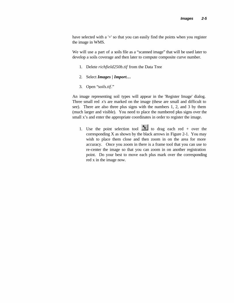
An image representing soil types will appear in the 'Register Image' dialog. Three small red x's are marked on the image (these are small and difficult to see). There are also three plus signs with the numbers 1, 2, and 3 by them (much larger and visible). You need to place the numbered plus signs over the small x’s and enter the appropriate coordinates in order to register the image.
1. Use the point selection tool to drag each red + over the corresponding X as shown by the black arrows in Figure 2-1. You may wish to place them close and then zoom in on the area for more accuracy. Once you zoom in there is a frame tool that you can use to re-center the image so that you can zoom in on another registration point. Do your best to move each plus mark over the corresponding red x in the image now.

2-6 WMS Tutorials
Figure 2-1: Moving + Marks in Registration Dialog
2.4.1 Conversion Calculator
We want to register images using the UTM x and y coordinates of each point, but we only know the latitude and longitude of the registration points. You can use the Convert Point… dialog to access the single point coordinate conversion dialog so that you can enter your coordinates in decimal degrees or degrees/minutes/seconds and convert to UTM (or any other) coordinates.
1. Choose the Convert Point… button from the Point #1 area on the Register Image dialog.

Images 2-7
2. Select Geographic NAD 83(US) from the Convert From: Horizontal System: drop down box.
3. Select UTM NAD 83(US) from the Convert To: Horizontal System: drop down box.
4. Set the Horizontal Units field to Meters
5. Select UTM Zone 12 114W to 108W from the Convert To: UTM Zone drop down box.
6. Set the Vertical System to Local and the Units field is Meters.
7. Find the latitude and longitude for Point 1 in Table 2-1.
8. Enter the appropriate Degrees, Minutes, and Seconds values for Point 1 in the edit boxes.
9. Choose the Convert button.
10. Select OK to exit the dialog.
The appropriate UTM x and y coordinates should appear in the X and Y edit boxes under Point 1 in the Register Image dialog.
1. Follow the same steps to convert the latitude and longitude coordinates of Points 2 and 3 to UTM coordinates (the settings in the conversion dialog should remain the same so that you only need to enter the coordinates for points 2 and 3).
2. Select OK on the Register Image dialog.
If the image appears distorted or crooked, you may have entered the coordinates incorrectly or placed the + marks inaccurately.
Table 2-1: Latitude and Longitude for Soils.tif
Point Longitude Latitude 1 112°28'55" W 38°41'06" N 2 112°28'38" W 38°34'36" N 3 112°19'49" W 38°34'34" N
1. Select File | New
2. Select OK to clear everything.

2-8 WMS Tutorials
2.5 Aerial Photographs
It is often useful to use aeria l photographs as background images in WMS. http://terraserver.microsoft.com has a large selection of satellite photos, aerial photographs, and images for locations throughout the United States. The aerial photographs from the TerraServer come with world files, simplifying the image registration process.
2.5.1 Download an Aerial Photograph from the Terraserver
To demonstrate TerraServer, we will download an aerial photograph of part of the Clear Creek watershed in Richfield, Utah.
If you are unable to connect to the internet at this point, or if you have difficulties obtaining the file(s) you can skip ahead to section 2.5.2 below and use the ClearCreek.jpg and ClearCreek.jgw files previously downloaded.
1. Go to http://terraserver.microsoft.com.
2. Type Joseph, UT in the Search TerraServer edit box shown in Figure 2-2.
Figure 2-2: Search TerraServer Edit Box and GO button
1. Choose GO (see Figure 2-2).
2. Choose the Topo Map 7/1/1980 for Joseph, Utah, United States as shown in Figure 2-3.

Images 2-9
Even though we are searching for an aerial photo, we will look at the topographic map, as it is easier to find specific features on.
Figure 2-3: Topo Map Image Link
1. Click on the 64 meter zoom bar, as shown in Figure 2-4.
Figure 2-4: 64-meter Zoom Bar
1. Click on the location as indicated by the X in the lower left of Figure 2-5 to zoom in.

2-10 WMS Tutorials
Figure 2-5: Zoom Location
1. Click on the South arrow, as shown in Figure 2-6, to pan to the South.
Figure 2-6: Pan South Arrow
1. Switch to the Aerial Photo view using the drop-down box as shown in Figure 2-7.

Images 2-11
Figure 2-7: View Drop-down Box
1. Choose the Download link as shown in Figure 2-8.
Figure 2-8: Download Link
You will be taken to a screen with your aerial photo and instructions for downloading both the image and the world file. Follow the instructions to save your image and the corresponding GIS World Coordinates file. To save the image file you will right-click on the image and save it. To save the world file follow the link on the lower-left side of the page. IMPORTANT: The world file must be saved as a text file and not an html file (the default). Be sure to change the file type to a text file when saving the world file.
Note that you should assign the image a name with a .jpg extension and the world file the same name, but with a *.jgw extension. If your browser appends any other extension to the file names, be sure to change them (it might put a .txt no matter what on the world file).
2.5.2 Import the Aerial Photograph Image
1. Switch to the Map module , if needed
2. Delete soilsreg.img from the Data Tree
3. Select Images | Import…
4. Select Jpeg image file (*.jpg, *.jpeg) from the Files of type drop-down box

2-12 WMS Tutorials
5. Open your downloaded file, or if you were unsuccessful then open “ClearCreek.jpg”
If you successfully downloaded the world file and it is named ClearCreek.jgw (note that when saving it may put a .txt extension on the file anyway) then it will open in WMS and be registered. If your world file has some other name, or does not end with .jgw then you can import it using the following three commands (skip these commands if it is already registered in WMS)
6. Choose the Import World File button on the Register Image dialog.
7. Open your downloaded world file (you might have to look for files with a .txt extension).
8. Select OK on the Register Image dialog.
You have successfully opened an aerial photograph and registered it in WMS.
2.6 Conclusion
In this tutorial, you were taught how to import several types of images into WMS. You learned how to georeference images and how to save the georeferenced images. In particular, you should know:
1. How to use geotiff files
2. What resampling an image means
3. How to use world files.
4. How to register scanned images
5. What a WMS image file is and how to save one
6. How to use aerial photographs

3 Basic Feature Objects
CHAPTER 3
Basic Feature Objects
Feature objects are points, lines, and polygons organized in coverages by different attribute sets such as drainage features, land use, soils, time travel paths, cross sections, etc. A synonymous word for coverage would be a layer (AutoCAD), theme (Arc View), or level (Micro Station). Simply put, a coverage contains points, lines, or polygons that have the same attribute set. For example, you don’t want to store land use polygons in the same coverage or layer as drainage basin or soil polygons.
The primary coverage in WMS is the drainage coverage, which holds drainage boundary polygons, stream lines, and outlet nodes. Most of the other coverages are secondary to the drainage coverage and are used to “map” other hydrologic parameters such as travel time or curve numbers. Feature objects are equivalent to GIS vector data and so importing from GIS databases is one important way to create coverages in WMS. Another important method for creating feature object coverages is to digitize directly from the screen, using a georeferenced image in the background as a guide.
3.1 Objectives
In this workshop you will learn the basics for creating and importing feature objects and managing different coverages. This includes the following:
1. Creating and editing feature objects
2. Feature object attributes

3-2 WMS Tutorials
3. Creating coverages and specifying attribute sets
4. Basic importing of shapefiles
5. Using images to create feature objects
6. Managing multiple coverages
3.2 Creating and Editing Feature Objects
The Terrain Data, Drainage, and Map modules are where the feature objects are created and manipulated. All feature objects are made from a set of points and the lines connecting the points. There are three main types of feature objects: points, arcs, and polygons. The following steps will teach you how to create and edit the different types of feature objects.
1. Switch to the Map module .
2. Select File | Open…
3. Open “FeatureObjects.img”
3.2.1 Creating Feature Arcs
1. Find the portion of the image labeled Vertices, Nodes, and Arcs.
2. Choose the Create Feature Arc tool
3. Single-click on the point labeled 1.
4. Double-click on point 2 to end the arc.
While you are creating a feature arc, you can hit Esc to cancel, Backspace to back up one vertex, Enter or single-click to make a vertex, and double-click to end the arc. When WMS creates an arc, each end is a node and all points in the middle are vertices.
1. Single-click at point 3, directly on top of the arc you just made.
Notice how WMS automatically links the new arc to the existing arc and creates a node at the point of intersection.
1. Double-click at point 4 to end the arc.
2. Single-click at point 5.

Basic Feature Objects 3-3
3. Double-click at point 6.
3.2.2 Snapping Arcs
Oftentimes you will have two arcs very close to each other that should share a common node, but do not. WMS has an option to snap these nodes together.
1. Find the portion of the image labeled Vertices, Nodes, and Arcs.
2. Choose the Select Feature Point/Node tool
3. Click on the node labeled 5.
4. Select Feature Objects | Clean…
5. Make sure the Snap selected nodes option is checked
6. Select OK
If you look down at the bottom of the WMS screen, you will notice the help window is prompting you to select a snapping point.
7. Click on the main arc near the point labeled 7.
WMS will not snap the arcs together because no vertex exists at the point you selected. To be able to snap the two arcs together, you must insert a vertex at this point.
3.2.3 Inserting Vertices
1. Choose the Create Feature Vertex tool .
2. Single-click on the arc where it is labeled 7.
A vertex is inserted here just as if you had clicked here when creating the arc originally. Now you can snap the two arcs together.
3. Choose the Select Feature Point/Node tool .
4. Click on the node labeled 5.
5. Select Feature Objects | Clean.
6. Make sure the Snap selected nodes option is checked.

3-4 WMS Tutorials
7. Select OK.
8. Select the vertex you just created.
WMS snaps the two arcs together and changes the vertex at point 7 to a node.
3.2.4 Deleting a Portion of an Arc
Now that the main arc you created has two nodes along its length, you can delete the center portion only.
1. Choose the Select Feature Arc tool
2. Select the portion of the arc between nodes 3 and 7
3. Select the Delete key to delete the arc
4. Choose the Create Feature Arc tool
5. Click on the node labeled 3
6. Double-click on the node labeled 7 to re-form the arc.
3.2.5 Converting Vertices to Nodes
WMS uses vertices and nodes for different purposes. Sometimes you will need to change a vertex to a node or a node to a vertex.
1. Choose the Create Feature Vertex tool .
2. Click on the arc somewhere between nodes 3 and 7.
3. Choose the Select Feature Vertex tool .
4. Select the vertex you just made.
5. Select Feature Objects | Vertex <-> Node
You should now see a red node at this location.
3.2.6 Converting Nodes to Vertices
Just as you can change vertices to nodes, you can change nodes to vertices.

Basic Feature Objects 3-5
1. Choose the Select Feature Point/Node tool .
2. Click on the node you just converted.
3. Select Feature Objects | Vertex <-> Node .
You can see that the node has been changed back to a vertex.
3.2.7 Building Polygons
Find the portion of the image labeled Polygons.
1. Choose the Create Feature Arc tool .
2. Single-click at the point labeled 1 on polygon A.
3. Single-click on points 2 through 10.
4. Single-click on point 1 again to end.
5. Trace polygon B in the same manner.
You should now have two closed loops made out of the arcs just created. They are not polygons at this time – they are still just arcs.
6. Select Feature Objects | Build Polygon
7. Select OK to use all the arcs.
The two polygons should now be drawn with a thick line instead of the thinner arc lines. Polygons are built from their constituent arcs.
3.2.8 Assigning Attributes
Each of the nodes, arcs, and polygons you created were created with default properties or attributes. WMS allows you to change the attributes of feature objects.
1. While holding the Shift key (multi-select) down select all 5 arc sections in the Vertices, Nodes, and Arcs portion of the image.
2. Select Feature Objects | Attributes…
A dialog will come up allowing you to choose whether you want the arcs to have the Generic, Stream, Lake, or Ridge attribute.

3-6 WMS Tutorials
3. Select the Stream option.
4. Select OK
The arcs should now be colored blue. Each arc portion should have a small blue arrow on it. These arrows show the way the stream you have created flows. The original direction you created the arc determines the way the stream flows now. Stream arcs should always be created from downstream to upstream. You should also be able to see that the lower node on the arc looks different now. WMS has automatically changed it to a drainage outlet instead of a generic node.
5. Choose the Select Feature Point/Node tool .
6. Double click on the lower node (now an outlet) .
A dialog comes up showing that the node now has the Drainage outlet attribute.
7. Select OK.
Just as you can change the attributes of arcs and nodes, you can change the attributes of polygons.
8. Choose the Select Feature Polygon tool .
9. Double-click anywhere inside Polygon A in the Polygons portion of the image.
10. Select the Drainage boundary type.
11. Select OK.
Polygon A should now be drawn in a thick colored line instead of a black one.
12. Double-click anywhere inside Polygon B.
13. Select the Lake/Reservoir type.
14. Select OK.
Polygon B should now be drawn in light blue.

Basic Feature Objects 3-7
3.3 Using Shape Files to Create Feature Objects
One of the most important features of WMS is the ability to automatically create feature objects using shapefiles. We will now import a streams shapefile and a basins shapefile and convert them to streams and basins.
1. Select File | New
2. Confirm that you want to clear all data
3. Switch to the GIS module .
You will import shapefile data differently depending on whether the computer you are working on has ArcInfo installed on it or not. For this tutorial, the two ways are basically equivalent. However, if you have ArcInfo installed, you have access to more data types and display options. First, you will import a shapefile without ArcInfo.
3.3.1 Without ArcInfo
1. Select Data | Add Shapefile Data.
2. Open “streams.shp”
In order for the shapefile to work correctly, streams.dbf and streams.shx must be located in the same directory as streams.shp. This is true for all shapefiles.
1. Choose the Select Shapes tool
2. Draw a box around all the shapes to select them all.
3. Select Mapping | Shapes -> Feature Objects.
This is the GIS to Feature Objects Wizard. It is used to map shapefile data to feature objects in WMS.
1. Choose Next.
The spreadsheet that is presented next shows each shapefile attribute in bold letters. In this file, you should see DRAINTYPE, LENGTH, SLOPE, etc. in bold letters. Underneath each attribute is a dropdown box containing the WMS attributes you can choose to map the shapefile attributes to.
1. Select Drainage Arc type from the dropdown box below DRAINTYPE.

3-8 WMS Tutorials
2. Select Stream length from the dropdown box below LENGTH.
3. Select Stream slope from the dropdown box below SLOPE.
4. Select Not mapped from the dropdown box below DMANNINGS.
This attribute cannot be mapped because there is not a corresponding WMS attribute available to map it to.
1. Select Stream basin id from the dropdown box below BASINID.
You can scroll through the mapping spreadsheet to see the value that is assigned to each attribute for each shape.
1. Choose Next.
2. Choose Finish.
You have now imported a shapefile containing streams and basins, converted all the shapes to WMS feature objects, and mapped data from the original shapefile to WMS attributes.
3.3.2 With ArcView
If you have ArcView (or ArcGIS) installed on your computer, you can choose to import shapefiles using ArcObjects capabilities. If you do not have ArcView then skip to the next section.
1. Select File | New.
2. Select OK to clear everything.
3. Select Data | Enable Arc Objects.
If the computer you are working on does not have ArcInfo installed, the Data menu will not change. If ArcInfo is installed, the previously dimmed menu items should become undimmed.
1. Select Data | Add Data .
2. If Data | Add Data is dimmed, skip to section 3.4.
3. Open “streams.shp”
In order for the shapefile to work correctly, streams.dbf and streams.shx must be located in the same directory as streams.shp. This is true for all shapefiles.

Basic Feature Objects 3-9
1. Choose the Select Features tool
2. Draw a box around all the shapes
3. Select Mapping | ArcObjects->Feature Objects.
4. This is the same GIS to Feature Objects Wizard you used in section 3.3.1. When you are finished mapping shapefile data to WMS attributes, choose Next, then Finish.
3.4 Creating Feature Objects Using Background Images
Another important feature of WMS is the ability to create feature objects using background images as guides. For instance, you may have a soil use map you want to read into WMS. The following procedure explains how this is done.
3.4.1 The Data Tree Window
First, you will need to create a new coverage by utilizing the Data Tree window on the right hand side of the WMS main window.
When in the Map module, the Data Tree displays the current coverages, and allows users to manage the coverages.
1. Select File | New.
2. Select OK to clear everything.
3. Switch to the Map module , if necessary
In the data tree window, you should see a folder entitled Map Data .
1. Click the + sign next to the Map Data folder.
Now you should see the default coverage listed (always a Drainage coverage when beginning a new project). From the Data Tree, you can manage the default coverage, make new coverages, delete coverages, edit coverage properties, and change the active coverage.
1. Right-click on the one existing coverage in the Data Tree
2. Select Rename
3. Enter PracticeDrainage for the new coverage name
3-10 WMS Tutorials
4. Right-click on the Map Data folder
5. Select New coverage
6. From the Coverage type dropdown box, select Soil Type
7. Notice that the Coverage name is automatically changed to Soil Type.
8. Select OK.
9. Click on the PracticeDrainage coverage.
You can see that this coverage shows up in color and bold, while the Soil Type drainage is in gray and regular font. This means that the PracticeDrainage coverage is the active coverage.
1. Select the Soil Type coverage to make it active.
2. Uncheck the box next to the PracticeDrainage coverage.
Now the PracticeDrainage coverage is not visible. Turn this coverage back on to make it visible again.
3.4.2 Reading in Images
Now that you have added a soil type coverage, you can read in the soils image.
1. Select Images | Import…
2. Open “soils.img”
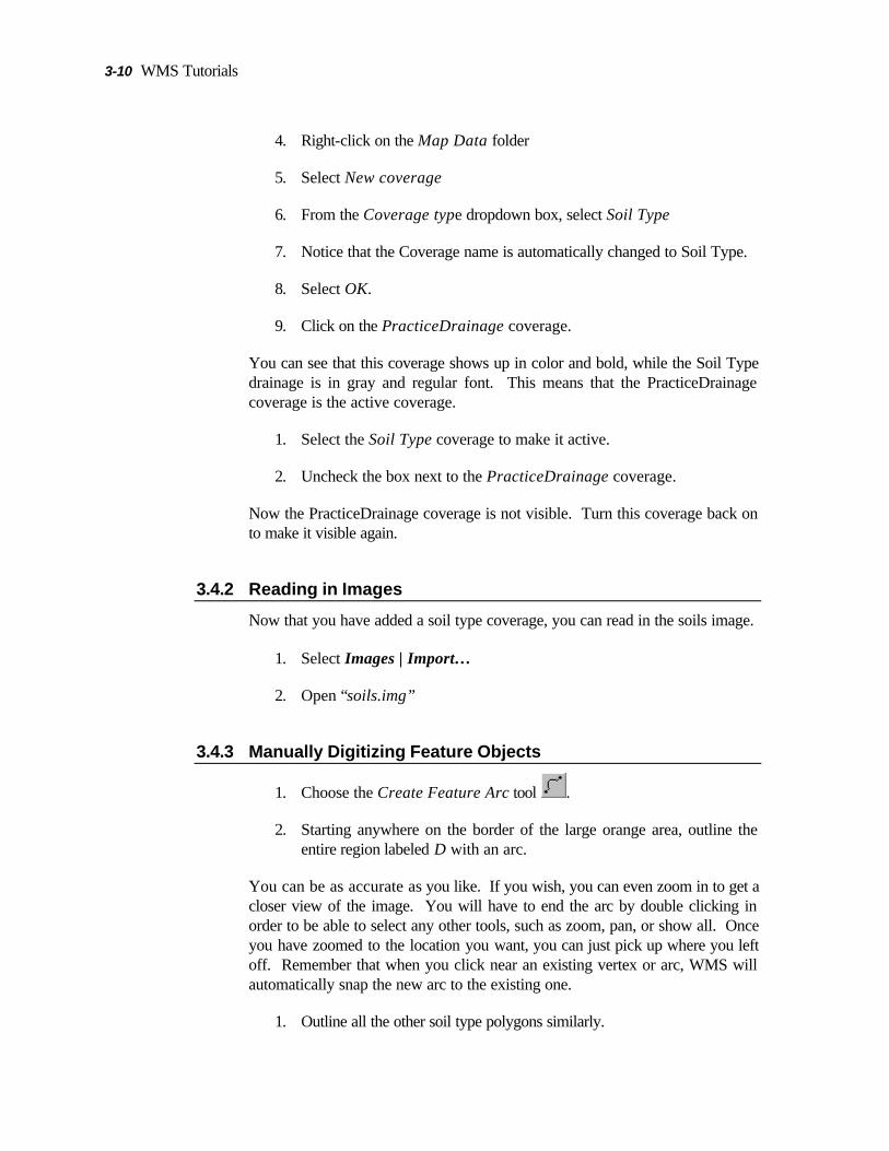
3.4.3 Manually Digitizing Feature Objects
1. Choose the Create Feature Arc tool .
2. Starting anywhere on the border of the large orange area, outline the entire region labeled D with an arc.
You can be as accurate as you like. If you wish, you can even zoom in to get a closer view of the image. You will have to end the arc by double clicking in order to be able to select any other tools, such as zoom, pan, or show all. Once you have zoomed to the location you want, you can just pick up where you left off. Remember that when you click near an existing vertex or arc, WMS will automatically snap the new arc to the existing one.
1. Outline all the other soil type polygons similarly.
Basic Feature Objects 3-11
2. Select Feature Objects | Build Polygon.
3. Select OK to use all the arcs.
Check to make sure that each soil use polygon is completely outlined. If one or more polygons do not build correctly, check to be sure that the arcs surrounding the polygons are completely closed.
3.4.4 Assigning Feature Polygon Attributes
Now that you have created the soil use polygons, you will need to assign the soil use attributes to the correct polygons.
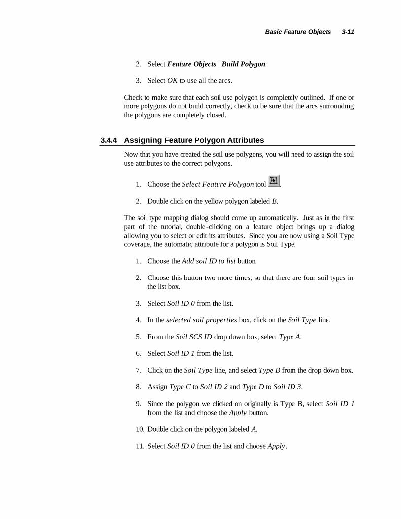
1. Choose the Select Feature Polygon tool .
2. Double click on the yellow polygon labeled B.
The soil type mapping dialog should come up automatically. Just as in the first part of the tutorial, double-clicking on a feature object brings up a dialog allowing you to select or edit its attributes. Since you are now using a Soil Type coverage, the automatic attribute for a polygon is Soil Type.
1. Choose the Add soil ID to list button.
2. Choose this button two more times, so that there are four soil types in the list box.
3. Select Soil ID 0 from the list.
4. In the selected soil properties box, click on the Soil Type line.
5. From the Soil SCS ID drop down box, select Type A.
6. Select Soil ID 1 from the list.
7. Click on the Soil Type line, and select Type B from the drop down box.
8. Assign Type C to Soil ID 2 and Type D to Soil ID 3.
9. Since the polygon we clicked on originally is Type B, select Soil ID 1 from the list and choose the Apply button.
10. Double click on the polygon labeled A.
11. Select Soil ID 0 from the list and choose Apply.
3-12 WMS Tutorials
12. Assign Soil ID 2 to all the polygons labeled C and Soil ID 3 to all the polygons labeled D.
13. Make sure each polygon has the proper Soil ID assigned by double clicking on each and checking the soil type in the Selected Soil Properties box.
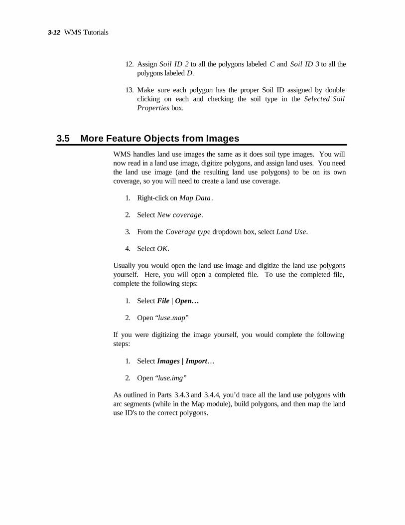
3.5 More Feature Objects from Images
WMS handles land use images the same as it does soil type images. You will now read in a land use image, digitize polygons, and assign land uses. You need the land use image (and the resulting land use polygons) to be on its own coverage, so you will need to create a land use coverage.
1. Right-click on Map Data .
2. Select New coverage.
3. From the Coverage type dropdown box, select Land Use.
4. Select OK.
Usually you would open the land use image and digitize the land use polygons yourself. Here, you will open a completed file. To use the completed file, complete the following steps:
1. Select File | Open…
2. Open “luse.map”
If you were digitizing the image yourself, you would complete the following steps:
1. Select Images | Import…
2. Open “luse.img”
As outlined in Parts 3.4.3 and 3.4.4, you’d trace all the land use polygons with arc segments (while in the Map module), build polygons, and then map the land use ID's to the correct polygons.

Basic Feature Objects 3-13
3.6 Display Options
WMS has many display options to help you tailor the look of your project to your needs. You can change options such as polygon colors, presence of nodes and vertices, and legends using the Display Options command.
1. Activate the Soil Type coverage by single-clicking on its name in the Data Tree
2. Select Display | Display Options…
3. On the Map tab, check the Color Fill Polygons box
4. Uncheck the Points/Nodes and Vertices boxes
5. Choose the Soil Type Display Options button
6. Select the first Soil ID listed in the list box and click on the color square to the right.
7. Choose a new color from the color palette.
8. Change the colors of the other soil groups uses if you desire
9. Select OK
10. Choose the General tab
11. Check the Soil Type Legend box
12. Select OK once again to exit the Display Options dialog.
You can continue to explore the display options if you wish. If you wanted to assign new colors to the land uses, you would need to make the land use coverage active before going back into the Display Options dialog.
3.6.1 Managing Coverages
Using the Data Tree window, you can choose to hide and/or show coverages and designate which coverage is the active coverage.
1. From the Data Tree window, toggle off the check boxes for the Drainage and the Soil Type coverages.
2. Click on the Land Use coverage so it will be active.

3-14 WMS Tutorials
Now only the land use coverage will be visible on the screen. The other coverages still exist; they simply will not show on the screen until you turn their visibility back on.
3.7 Conclusion
In this workshop you should have learned the basics for creating and importing feature objects and managing different coverages. Both these concepts are central to your understanding of WMS. You should now be able to:
1. Create and edit feature objects
2. Set feature object attributes
3. Create coverages and specify coverage attribute sets
4. Import shapefiles
5. Use images to create feature objects
6. Manage multiple coverages
4 Advanced Feature Objects
CHAPTER 4
Advanced Feature Objects
In the previous workshop you learned how feature points, lines, and polygons are created and organized into coverages. In this workshop you will continue to learn about the creation and editing of feature objects, with a focus on creating drainage coverages, the primary coverage used by WMS to develop watershed models.
4.1 Objectives
In this workshop you will learn the basics for creating and importing feature objects and managing different coverages. This includes the following:
1. Using feature object drainage coverages for watershed delineation
2. Advanced feature object editing functions
3. Assigning appropriate feature object attributes
4. Importing and editing feature objects from DXF data
This tutorial demonstrates how feature objects alone can be used to define hydrologic models. Feature objects may be digitized on-screen using a registered image, or imported as a shape file from an Arc/Info or ArcView layer. Using the drainage coverage type, features can be converted to streams, outlets, and basins to represent the watershed being modeled.

4-2 WMS Tutorials
4.2 Creating a Watershed from Scratch with Feature Objects
By using a combination of stream arcs, outlet nodes, and basin polygons, you can develop an entire watershed even without the use of a digital terrain model. The watershed can be to scale or a schematic. Of course, if it were not to scale, polygon areas and stream lengths would not be valid for your hydrologic model.
In this section of the tutorial you will create the Aspen Grove watershed from an image of a scanned paper map with clearly marked streams and basin boundaries.
1. Switch to the Map module .
2. Select File | Open…
3. Open “aspentrc.img”
You should see a portion of a USGS quad map with basin boundaries outlined in red and the stream network in black.
4.2.1 Creating Basin Boundaries
We will begin by creating the basin boundaries, but it does not matter whether the basins or streams are created first.
1. Choose the Create Arcs tool .
2. Select Feature Objects | Attributes…
3. Make sure that the arc type is Generic and Select OK.
4. Beginning at the outlet point (lower right) trace out the entire watershed boundary. You do not need to follow every detail; take as much time as you want. End by double-clicking near the same point where you began.
5. Now create each of the other three sub-basin boundary arcs on the interior of the watershed. Begin by clicking on a point near the junction in the center of the watershed and ending by double-clicking near the intersection of the arc previously created for the exterior boundary.

Advanced Feature Objects 4-3
4.2.2 Creating the Stream Network
The stream network is created in much the same way the basin boundaries were. The only thing to note is that in the upper basin the basin boundary comes very close to the stream. You will need to zoom in on this region in order to avoid conflicts with the snapping tolerance.
1. Select Feature Objects | Attributes…
2. Choose the Stream feature arc type.
3. Select OK.
4. Create the main channel from the outlet of the watershed to the outlet point for the two upper basins. Begin by clicking near enough to the boundary arc at the outlet so that it snaps to it and end by double - clicking on the basin junction point.
5. Create the two branches of the lower basin by clicking on a point near the stream arc just created and double -clicking at the most upstream point of the branches in the image.
NOTE: As you create new vertices on stream arcs you should always do so from downstream to upstream.
1. Choose the Zoom tool .
2. Zoom in on the region shown in Figure 4-1.
Figure 4-1: Junction of Main Channel in Aspen Grove Watershed.
1. Choose the Create Arcs tool .

4-4 WMS Tutorials
2. Create the initial portion of each portion of the stream by clicking on the junction point (intersection of red boundary lines in the image) and going as far upstream as is possible on the zoomed image. End by double -clicking.
You needed to zoom in order to avoid conflicts with the auto-snapping feature. If you do click too close to an existing arc you will get a message that the stream is illegal and you will need to try again.
You can end the stream at one location and then continue defining after zooming out by beginning at the point where you left off.
1. Select Display | View | Previous View
2. Finish defining each branch. Begin the branch by clicking near the point you left off with and ending by double clicking at the terminal point of the stream.
In order to define separate basins at the junction point you will need to convert the node at the junction to an outlet node.
1. Choose the Select Feature Point/Node tool
2. Select the junction point in the center of the watershed corresponding to the intersection of the streams and the sub-basin boundary arcs that you just created.
3. Select Feature Objects | Attributes…
4. Change the attribute to Drainage outlet.
5. Select OK.
4.2.3 Building Polygons
At this point the watershed boundaries are only arcs. In order for them to become polygons you must create the polygon topology.
1. Choose the Select Polygon tool .
2. Select Feature Objects | Attributes.
3. Change the attribute to Drainage boundary. Select OK.
4. Choose the Select Feature Line Branch tool .

Advanced Feature Objects 4-5
5. Select Edit | Select All.
6. While holding down the Shift key, select the southern-most stream arc. This un-selects the stream arcs and leaves the remainder selected for use in polygon generation.
7. Select Feature Objects | Build Polygon.
4.2.4 Updating Geometric Parameters
1. Select Display | Display Options…
2. Turn on the Color fill polygons option.
3. Select OK.
In order to transfer the basin area and stream lengths, and to compute them in appropriate units for hydrologic modeling you need to compute the basin data. This will make it possible to use the polygon area in any of the hydrologic modeling interfaces.
1. Select Feature Objects | Compute Basin Data… This command computes areas, perimeters, and centroids for each of the sub-basins and assigns these values to the hydrologic modeling tree.
2. In the Units Dialog select the Current Coordinates… button.
3. Make sure the Horizontal and Vertical units are Meters (the base units were UTM meters).
4. Select OK.
5. Set the Basin Areas units to Square miles.
6. Set the Distances units to Feet.
7. Select OK to compute the sub-basin data.
4.3 Cleaning
Since you changed some display settings in the last part of the tutorial, you need to completely exit out of WMS and restart the program before continuing.
1. Switch to the Map module

4-6 WMS Tutorials
2. Select File | Open.
3. Open “streams.img”
For this file to open properly, richfield250a.tif must be located in the same folder as streams.img.
1. Choose the Zoom tool .
2. Using the zoom tool, draw the zoom window shown in Figure 4-2.
Figure 4-2: Zoom Window
3. As explained in the previous section, digitize the streams and lakes shown in Figure 4-3. Start at the junction the red arrow points to. When you come to a lake, simply trace a stream straight through it.

Advanced Feature Objects 4-7
Figure 4-3: Stream Network and Beginning Junction
4.3.1 Turning Off Image Display
You can now turn off the image by completing the following steps.
1. Expand the Map Data folder in the Data Tree if necessary
2. Toggle the visibility check box next to the “streams.img” image off
4.3.2 Importing a Shapefile
1. Select File | Open
2. Open “basins.shp”
3. Select OK
There are some problems with this set of basins and streams. For example, none of the basin junctions meet up with the corresponding stream junctions. Fixing problems like these is called 'cleaning' and is demonstrated in the following steps.
1. Choose the Zoom tool .
2. Zoom in on the main outlet (at the bottom of the watershed). You will have to get quite close.
4-8 WMS Tutorials
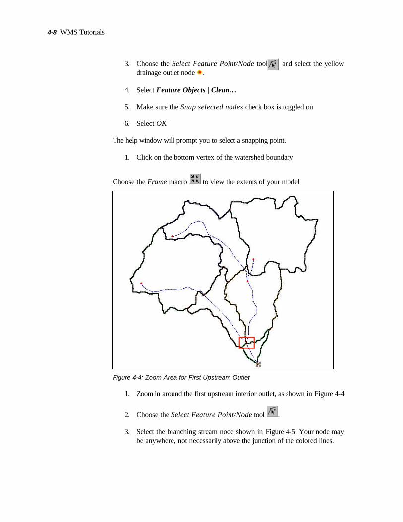
3. Choose the Select Feature Point/Node tool and select the yellow drainage outlet node .
4. Select Feature Objects | Clean…
5. Make sure the Snap selected nodes check box is toggled on
6. Select OK
The help window will prompt you to select a snapping point.
1. Click on the bottom vertex of the watershed boundary
Choose the Frame macro to view the extents of your model
Figure 4-4: Zoom Area for First Upstream Outlet
1. Zoom in around the first upstream interior outlet, as shown in Figure 4-4
2. Choose the Select Feature Point/Node tool .
3. Select the branching stream node shown in Figure 4-5 Your node may be anywhere, not necessarily above the junction of the colored lines.

Advanced Feature Objects 4-9
Figure 4-5: Branching Stream Node
1. Select Feature Objects | Clean…
2. Make sure the Snap selected nodes checkbox is selected.
3. Select OK.
4. Select the junction of the three basins as the snapping point by clicking on it.
This node also needs to be changed to a drainage outlet.
1. Choose the Select Feature Point/Node tool .
2. Select the node.
3. Select Feature Objects | Attributes…
4. Select the Drainage outlet radio button.
5. Select OK.
6. Use the Frame macro to zoom out.
7. Zoom in around the left stream branch and basin junctions, as shown in Figure 4-6.

4-10 WMS Tutorials
Figure 4-6: Left Stream Branch Zoom Area
1. Choose the Select Feature Arc tool .
Figure 4-7: Arcs to Clean
1. Select the stream arc and the basin arc it crosses
2. Select Feature Objects | Clean…
3. Make sure the Intersect selected arcs check box is selected
4. Select OK
The two arcs are intersected and a node is placed at the intersection point. As before, this node needs to be an outlet.

Advanced Feature Objects 4-11
1. Choose the Select Feature Point/Node tool
2. Select the node
3. Select Feature Objects | Attributes…
4. Select the Drainage outlet radio button
5. Select OK
6. Use the Frame macro to zoom out
Zoom in around the right stream branch and basin junctions as shown in
7. Figure 4-8
Figure 4-8: Zoom Area for Right Stream Branch
1. Choose the Select Feature Arc tool .
2. Select the right branch of the stream arc and the basin arc it crosses as shown in Figure 4-9.

4-12 WMS Tutorials
Figure 4-9: Stream Branches and Basin Arcs to Clean
1. Select Feature Objects | Clean…
2. Make sure the Intersect selected arcs check box is selected.
3. Select OK.
The two arcs are intersected and a node is placed at the intersection point. As before, this node needs to be an outlet.
1. Choose the Select Feature Point/Node tool .
2. Select the node.
3. Select Feature Objects | Attributes…
4. Select the Drainage outlet radio button.
5. Select OK.
6. Choose the Select Feature Arc tool .
7. Select the left branch of the stream arc and the basin arc it crosses as shown in Figure 4-9.
8. Select Feature Objects | Clean...
9. Make sure the Intersect selected arcs check box is selected.
10. Select OK.

Advanced Feature Objects 4-13
The two arcs are intersected and a node is placed at the intersection point. As before, this node needs to be an outlet.
1. Choose the Select Feature Point/Node tool .
2. Select the node.
3. Select Feature Objects | Attributes…
4. Select the Drainage outlet radio button.
5. Select OK.
6. Use the Frame macro to zoom out.
The set of streams and basins is now cleaned and ready to be used in hydrologic analysis.
4.4 Feature Objects from CAD Data
You may have CAD data available. DWG and DXF data can be automatically converted to feature objects in WMS.
1. Select File | New
2. Switch to the Map module
3. Select File | Open…
4. Open “af.dwg”
5. Select CAD | CAD -> Feature Objects
The dialog that opens shows a check mark for each layer that will be converted to feature objects. We will convert all layers and accept the default coverage type (which should be Drainage) and name (which should be CAD layers).
6. Select OK
7. Select OK to accept the coverage type and name.
8. Select CAD | Display Options…
9. Toggle off the check box at the top labeled Display CAD data

4-14 WMS Tutorials
10. Select OK
Because these lines were created in AutoCAD we can’t be sure (and in most cases they won’t) that the streams are created using the WMS conventions for direction. In order to fix any such problems you can use the Reorder Streams command. By selecting the most downstream node in a stream network and invoking the Reorder Streams command, you tell WMS to ensure that all arcs are ordered downstream to upstream from the selected point.
1. Choose the Select Feature Point/Node tool
2. Select the left-most node in the interior of the basin (the left-most node on the portion that forms a network inside of the arcs forming a boundary).
3. Select Feature Objects | Reorder Streams
4. Choose the Select Feature Line Branch tool
5. Select the arc attached to the left-most node (the node that was just used to reorder streams).
6. Select Feature Objects | Attributes…
7. Select the Stream type and Select OK.
Each stream now flows the proper direction, toward the one drainage outlet at the left of the stream network. This outlet needs to be snapped to the basin boundary.
1. Choose the Select Feature Point/Node tool
2. Select the drainage outlet
3. Select Feature Objects | Clean…
4. Make sure Snap selected nodes is checked.
5. Select OK.
6. Choose the node on the basin boundary closest to the drainage outlet.
7. Select Feature Objects | Build Polygon.
8. Select OK.

Advanced Feature Objects 4-15
This set of streams and basins is now properly ordered and connected and is ready to be used for hydrologic analysis.
4.5 Conclusions
In this workshop you should have learned how to do the following:
1. Use feature object drainage coverages for watershed delineation
2. Advanced feature object editing
3. Assign appropriate feature object attributes
4. Import and edit feature objects from DXF data

5 DEM Basics
CHAPTER 5
DEM Basics
Digital Elevation Models (DEMs) are the most commonly available digital elevation source and therefore an important part of using WMS for watershed characterization. A DEM is a rigid data structure that contains a two-dimensional array of elevations where the spacing between elevations is constant in the x and y directions. In the US DEMs are downloadable from the internet at 30-meter (1:24,000 map series) and 90-meter (1:250000 map series). The USGS has recently deployed the National Elevation Dataset which is a continuous elevation map at 30-meter resolution. Blocks of 100 MB or less can be downloaded for free from the NED website.
The Arc/Info ASCII grid format is common throughout the GIS world and is common outside the US. The basics of downloading, importing, editing, and displaying DEMs will be demonstrated in this workshop. Actually using the DEM for watershed delineation is the subject of the next workshop.
5.1 Objectives
In this workshop you will learn the basics of importing, viewing and preparing DEMs for automated watershed delineation. This includes the following:
1. Importing USGS DEMs from different formats
2. Tiling multiple DEMs together
3. Editing DEM elevations

5-2 WMS Tutorials
4. Setting DEM display options
5.2 Getting DEMs from the Internet
In this part of the tutorial, you will learn how to download DEM data from WebMET, The Meteorological Resource Center, at http://www.webgis.com, from GeoCommunity/GIS Data Depot at http://www.gisdatadepot.com or http://www.geocomm.com, and from the National Elevation Data website at http://gisdata.usgs.net/ned/. Instead of book-marking all these sites, you can bookmark http://www.emrl.byu.edu/gsda. This site contains links to many sites where you can get DEM data.
If you do not have an internet connection you can still work through this tutorial, using the files which have been downloaded already and placed in the tutorials directories, or you may want to skip ahead to section 5.3 now.
5.2.1 WebMET
WebMET provides old style DEMs – 7.5 minute USGS quad DEMs.
1. Go to www.webgis.com
2. Select the United States (7.5m) link in the Terrain Data area
3. Click on Utah (UT)
4. Choose the List Counties Alphabetically link found underneath the map
5. Select Sevier County
6. Scroll down until you see Trail Mountain
7. Select the Trail Mountain link
8. Your browser should allow you to save the file to your computer. Choose a spot to save it in
9. Unzip the file using WinZip or another unzipping utility. The unzipped file should have a .dem extension
You are now able to use this DEM directly in WMS. If you are not connected to the internet or you were unsuccessful downloading the Trail Mountain DEM then you can use the file (trailmountain.dem) included with the tutorial data.

DEM Basics 5-3
1. In WMS, switch to the Terrain Data module
2. Select File | Open…
3. Open the *.dem file you just unzipped
4. Select OK
WMS should read in the DEM, and it should look similar to other .dem files you have read in.
5.2.2 GeoCommunity/GIS Data Depot
The GeoCommunity/GIS Data Depot website provides the new style SDTS DEMs. If you want to learn more about the SDTS style of DEMs, the GIS Data Depot has an article you can read at http://data.geocomm.com/sdts/ (Aug 8, 2002). You will be asked to create a GeoCommunity account in order to download data from this website.
1. Go to www.gisdatadepot.com
2. From the list of topics on the left column, click on USGS DEMs or scroll down until you see the heading USGS DEMs on the main page
3. Scroll down to DOWNLOAD DEM DATA HERE and click on the link
4. Scroll down and select Utah
5. Select Sevier County
6. Select Digital Elevation Models (DEM) – 24K
7. Scroll down to Trail Mountain, UT (38112e4) and click on the green download button
8. Log in or create a GeoCommunity account
9. Select the 1666653.DEM.SDTS.TAR.GZ (30 meter) link.
10. Save the file on your computer. If you are unsuccessful doing this you will find the downloaded file included and unzipped with the WMS tutorial data. It has been unzipped into the trailmtnsdtsdem directory.
11. Use an unzipping utility such as Winzip to unzip the downloaded file.
If you wish, you can try to open up this DEM in WMS.

5-4 WMS Tutorials
1. Select File | New
2. Select OK to clear everything.
3. Switch to the Terrain Data module .
4. Select File | Open…
5. Open any one of the .ddf files you just unzipped. It does not matter which of the several .ddf files you pick, WMS will automatically determine which files contain the necessary data.
6. Select OK
WMS should read in the DEM, and it should similar to other .dem files you have read in. If you are interested in experimenting with a DEM that has a higher resolution you can load the 10-meter DEM for the Trail Mountain quadrangle. You will find the downloaded (or you can download for yourself) 10 meter SDTS DEM in the 1699603.DEM.SDTS.TAR.GZ file.
5.2.3 USGS National Elevation Dataset
The USGS National Elevation Dataset (NED) provides continuous 1:24,000-scaled DEM data for all of the contiguous US and 1:63,360-scale DEM data for Alaska. To access this data, complete the following steps:
1. Go to http://seamless.usgs.gov, then click on the View and Order Data Sets button. (You could also go to http://www.emrl.byu.edu/gsda and click on DEM, then click on OBTAIN DEM DATA, then click on the CLICK HERE to obtain 1:24,000 (30m) DEM data from the National Elevation Database.)
2. Choose the Find tool (the binoculars) and type in Richfield
3. Click the Find String button
4. Scroll down to number 6 (Richfield, Sevier, Utah) and click on it
5. Turn on the Streams and Waterbodies Layers and click Refresh Map. You may have to scroll the legend on the right side of the map down so you can see the Refresh Map button.
6. Use the Zoom tool to zoom in around the area shown in Figure 5-1

DEM Basics 5-5
Figure 5-1: Zoom Window
1. Use the Zoom tool to zoom in again around the area shown in Figure 5-2
Figure 5-2: Zoom Window
1. Under the Download section, choose the Download Area tool
2. Make the rectangle shown in Figure 5-3. An order confirmation page should come up.

5-6 WMS Tutorials
Figure 5-3: Download Selection Window
1. Select the Modify Data Request button.
2. Uncheck the 1/3” NED, the NLCD, and the SRTM options.
3. Select GridFloat from the Data Format drop down box next to NED - National Elevation Dataset.
4. Select the Save Changes & Return to Summary button.
5. Select the Download link when the request summary page displays again. Save the .zip file to a location where you can unzip it.
6. Use WinZip, or any unzipping utility to unzip the file that you download. If you were not successful downloading the DEM data you can use the richfieldNED.zip file found with the tutorial data, which has been unzipped into the NED directory.
If you wish, you can try to open up this DEM in WMS.
1. Select File | New
2. Select OK to clear everything
3. Switch to the Terrain Data module .
4. Select File | Open…
5. Open “demfloat.hdr” (this is one of the files you just unzipped, or you can open it from the NED subdirectory).

DEM Basics 5-7
6. Select OK
WMS should read in the DEM, and it should be similar to other DEM files you have read in.
5.2.4 Arc/Info ASCII Grid Format DEMs
Many agencies manage their data with Arc/Info software, so you will often need GIS data in the ASCII grid format so that it can be used in WMS.
1. Select File | New
2. Select OK to clear everything
3. Select File | Open…
4. Open “ArcInfoDEM.asc”
5. Select OK
The Arc/Info grid is read in just as any other DEM.
5.3 Merging DEMs
The area you are studying may lie across two or more DEM quads. WMS is able to merge multiple DEM files that span quad sheets. To see how this works, complete the following steps:
1. Select File | New
2. Select OK to clear everything
3. Select File | Open…
4. Find and multi-select josephpeak.dem, redridge.dem, marysvalecanyon.dem, and trailmountain.dem.
5. Choose Open
You will be taken to the Importing USGS DEMs manager. The area covered by the DEM you have selected will be colored in a box near the center of the dialog. The boundaries of your DEM area will show up in the four edit boxes.
By multi-selecting the DEMs you want, you can read in all the quads you need at the same time. WMS is able to read in an unlimited number of DEMs at a time (unless your computer runs out of memory). You can read in multiple
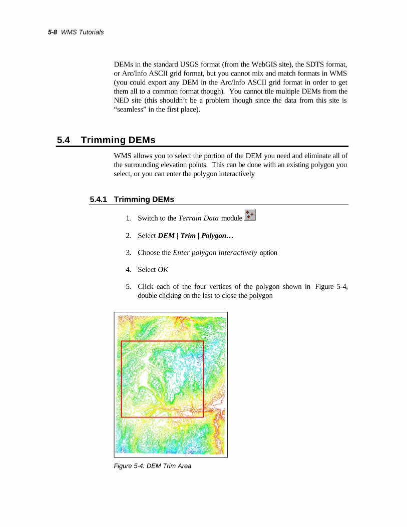
5-8 WMS Tutorials
DEMs in the standard USGS format (from the WebGIS site), the SDTS format, or Arc/Info ASCII grid format, but you cannot mix and match formats in WMS (you could export any DEM in the Arc/Info ASCII grid format in order to get them all to a common format though). You cannot tile multiple DEMs from the NED site (this shouldn’t be a problem though since the data from this site is “seamless” in the first place).
5.4 Trimming DEMs
WMS allows you to select the portion of the DEM you need and eliminate all of the surrounding elevation points. This can be done with an existing polygon you select, or you can enter the polygon interactively
5.4.1 Trimming DEMs
1. Switch to the Terrain Data module
2. Select DEM | Trim | Polygon…
3. Choose the Enter polygon interactively option
4. Select OK
5. Click each of the four vertices of the polygon shown in Figure 5-4, double clicking on the last to close the polygon
Figure 5-4: DEM Trim Area

DEM Basics 5-9
5.5 Displaying DEMs
5.5.1 Contour Options
WMS has several options for displaying DEMs. First, you can change the contour display options by following these steps:
1. Select Display | Display Options…
2. Select the DEM tab and choose the Contours… button. Make sure you are on the DEM tab, not the TIN tab
3. Under Contour Interval, change the number of contours in the edit box to 10
4. Select OK twice
You can see that there are fewer contours and they are spread farther out now.
1. Select Display | Display Options…
2. Select the DEM tab and choose the Contours button
3. Under Contour Method, select the Color fill between contours radio button
This option will 'color in' the contours.
1. Under Bold and Label check the Display Legend checkbox
2. Select OK twice
You can go back into the Contour options dialog and explore more of the contour display options if you wish.
5.5.2 Point Display Step
Next you will explore the point display step option:
1. Select Display | Display Options…
2. Select the DEM tab
3. Change the number in the Point display step edit box to 4
4. Select OK

5-10 WMS Tutorials
You can see that the display is not as smooth now.
1. Select Display | Display Options…
2. Select the DEM tab
3. Change the Point display step to 12
4. Select OK
5. Change the Point display step back to 2
Raising the point display step will allow your DEM display to refresh faster, especially if your computer is slow. However, this will also result in less accuracy when you start using the DEM for hydrologic computations.
5.5.3 Hill Shade and Light Angle
Now you will explore the hill shade and light angle options:
1. Select Display | Shade
The DEM is now shaded and it is easy to visualize the elevations.
1. Select Display | Light Angle
2. Click on one of the black or gray sections of the globe
3. Select OK
4. Select Display | Shade
Changing the light angle changes the way the shading option displays the DEM. You can play around with the light angle to accentuate the elevations that are most important for you to see.
5.5.4 Views
Many times it is easier to see the DEM elevations from another view other than the straight overhead birds' eye view.
1. Select Display | View-Oblique View. (Alternatively, you can also
select the Perspective View macro .)

DEM Basics 5-11
It is now much easier to see the changes in elevation on the DEM. If the elevation relief cannot be seen clearly, you can change the Z-magnification to accentuate the elevation relief.
1. Select Display | View-Z Magnification
2. Enter 3 in the edit box.
3. Select OK
The image will redraw on its' own. You will be able to see the elevation relief better now.
5.6 Conclusion
DEM data for the United States is found in several places on the internet. Data is available for most areas of the U.S. and some parts of other countries. DEM data is very useful for delineating watersheds in WMS.
In this workshop you should have learned how to do the following:
1. Importing USGS DEMs from different formats
2. Tiling multiple DEMs together and editing DEM elevations
3. Setting DEM display options


6 DEM Delineation
CHAPTER 6
DEM Delineation
Watershed delineation from DEMs is straightforward and relatively simple, providing the project area is not entirely flat or completely dominated by man-made structures (you can’t expect the DEM method to work if there is no relief in the DEM elevations themselves).
Because some DEMs do not contain enough resolution to accurately incorporate roadways, canals, and other man-made structures in the delineation, you may need to alter the delineation either by using additional stream arcs, or by editing the elevations. This process, including how to alter delineations when necessary is the subject of this workshop.
6.1 Objectives
In this workshop you will learn the basics of importing, viewing and preparing DEMs for automated watershed delineation. This includes the following:
1. Computing flow paths and flow accumulations
2. Delineating watersheds from DEMs
3. Delineating sub-basins within a watershed
4. Using feature line streams to modify delineations

6-2 WMS Tutorials
6.2 Importing DEM Data
The first step in delineating a watershed is to import one or more DEMs.
To read in a set of eight 30-meter DEMs from the 1:24000 series, complete the following steps:
1. Select File | Open…
2. Open “covefort.dem”
3. From the Importing USGS DEMs dialog, add the following seven DEMs just as you did in the previous tutorial:
4. josephpeak.dem
5. marysvalecanyon.dem
6. mountbelknap.dep
7. mountbrigham.dem
8. polemountain.dem
9. redridge.dem
10. trailmountain.dem
11. Enter a thinning factor of 3 in the Thinning factor edit field
Thinning the resolution of the DEMs will reduce the density of elevation points so that your computer will process the DEM data faster. The resolution of points in the 30-meter DEMs is too dense for the purposes of this tutorial, so you will not lose any accuracy by thinning.
1. Select OK
6.2.1 Trimming the DEM
1. Select DEM | Trim | Polygon…
2. Select the Enter Polygon Interactively option
3. Select OK
4. Trace around the area formed by the polygon shown in Figure 6-1
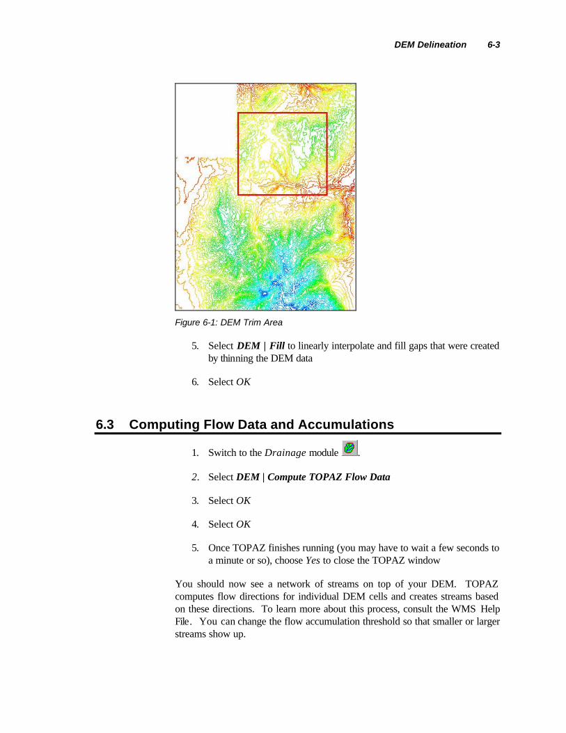
DEM Delineation 6-3
Figure 6-1: DEM Trim Area
5. Select DEM | Fill to linearly interpolate and fill gaps that were created by thinning the DEM data
6. Select OK
6.3 Computing Flow Data and Accumulations
1. Switch to the Drainage module .
2. Select DEM | Compute TOPAZ Flow Data
3. Select OK
4. Select OK
5. Once TOPAZ finishes running (you may have to wait a few seconds to a minute or so), choose Yes to close the TOPAZ window
You should now see a network of streams on top of your DEM. TOPAZ computes flow directions for individual DEM cells and creates streams based on these directions. To learn more about this process, consult the WMS Help File. You can change the flow accumulation threshold so that smaller or larger streams show up.

6-4 WMS Tutorials
1. Choose the Frame macro
2. Select Display | Display Options…
3. Select the DEM tab
4. Change the Min Accumulation For Display to 0.2 and Select OK
You should now see a more detailed network of streams.
1. Select Display | Display Options…
2. Select the DEM tab
3. Change the Min Accumulation For Display to 1.5 and Select OK
You should now see only a few large stream branches.
6.3.1 Drawing Flow Paths
WMS can draw a flow path from any point on a watershed to the eventual outlet.
1. Choose the Flow Path tool
2. Click on any portion of the DEM and see the resulting flow path
3. After you have drawn a few flow paths, choose the Refresh tool to clean up the image.
6.4 Delineating Watersheds from DEMs
WMS uses the data computed by TOPAZ to delineate watershed basins.
6.4.1 Creating the Basin Outlet
1. Zoom in around the area shown in Figure 6-2.

DEM Delineation 6-5
Figure 6-2: DEM Zoom Area
1. Choose the Create Outlet Point tool
2. Place the node just upstream of the branch junction shown in Figure 6-3
Figure 6-3: Drainage Outlet Location
1. Choose the Frame macro
2. Select DEM | DEM -> Stream Arcs

6-6 WMS Tutorials
3. Turn on both the Display stream feature arc creation option and the Use feature points to create streams options
4. Set the Threshold value to 0.3
5. Select OK.
By creating a point on a lower stream branch, you defined a watershed outlet. WMS then used the flow direction and accumulation data from TOPAZ to convert the TOPAZ streams into stream feature arcs.
6.4.2 Defining a Basin
These stream feature arcs computed by TOPAZ can now be used to define basins.
1. Select DEM | Define Basins
Now that the basins have been delineated, you can convert them to feature polygons and compute the basin data.
1. Select DEM | Basins->Polygons
2. Select DEM | Compute Basin Data…
3. Select OK on the Units dialog
4. Select Display | Display Options…
5. Select the Drainage Data tab
6. Check the Show Units, Basin Areas, and Basin Slopes options
7. Select OK.
Using DEM data, you have delineated a watershed and stream network. Because the DEM contains elevation data, your model can be used to compute data such as slopes, stream lengths, areas, etc. It is not just a schematic of the watershed.
6.5 Creating Sub-Basins
In previous watershed models you have looked at, each watershed was divided into several smaller sub-basins. You will learn how to create these interior sub-basins in this part of the tutorial. You should always finish delineating the major
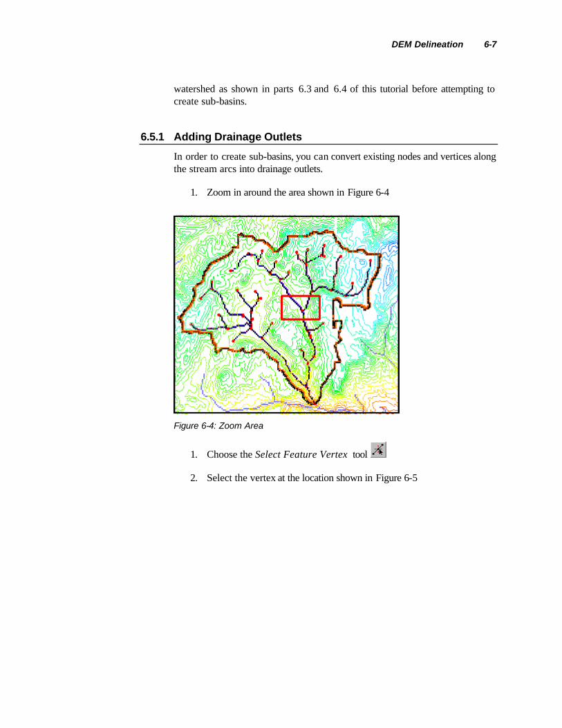
DEM Delineation 6-7
watershed as shown in parts 6.3 and 6.4 of this tutorial before attempting to create sub-basins.
6.5.1 Adding Drainage Outlets
In order to create sub-basins, you can convert existing nodes and vertices along the stream arcs into drainage outlets.
1. Zoom in around the area shown in Figure 6-4
Figure 6-4: Zoom Area
1. Choose the Select Feature Vertex tool
2. Select the vertex at the location shown in Figure 6-5
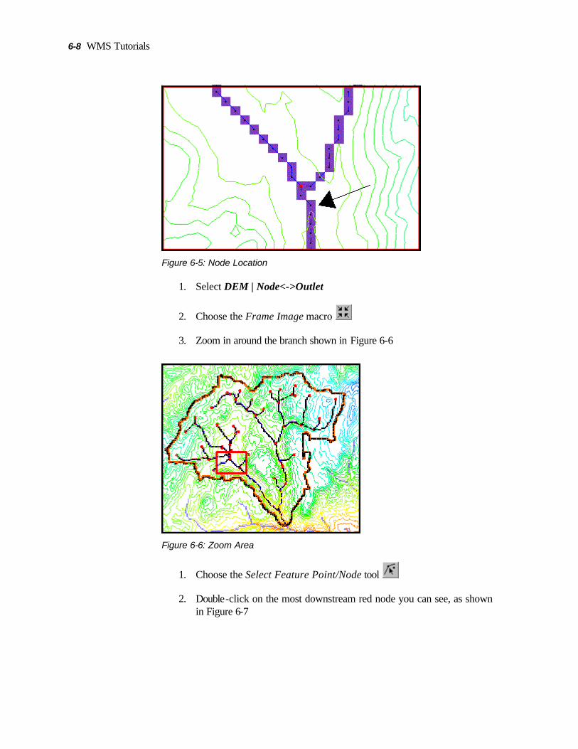
6-8 WMS Tutorials
Figure 6-5: Node Location
1. Select DEM | Node<->Outlet
2. Choose the Frame Image macro
3. Zoom in around the branch shown in Figure 6-6
Figure 6-6: Zoom Area
1. Choose the Select Feature Point/Node tool
2. Double-click on the most downstream red node you can see, as shown in Figure 6-7

DEM Delineation 6-9
Figure 6-7: Change the indicated node to an outlet.
3. Select the Drainage outlet option
4. Select OK
5. Select the Frame Image macro
6.5.2 Defining Sub-Basins
1. Select DEM | Define Basins
2. Select DEM | Basins->Polygons
3. Select DEM | Compute Basin Data…
4. Select OK
Notice that on the left basin, where you changed the existing node to an outlet, the basin was divided into two smaller sub-basins automatically. On the right basin, where you added an outlet below the stream junction, only one basin was created.
6.6 Adding a Stream Arc and Redefining Basins
Sometimes you will need to add stream arcs to your basin to represent man-made objects such as roads. Roads often disrupt the natural flow of watersheds and water collects along roads just as it collects in a stream. This

6-10 WMS Tutorials
collected water needs to be "added" into your watershed in order to properly model the real-life situation.
1. Select File | Open…
2. Open “richfield250a.tif”
3. Switch to the Map module
4. Choose the Zoom tool
5. Zoom in along the road as shown in Figure 6-8.
Figure 6-8: Road Zoom Area
1. Choose the Create Feature Arc tool
2. Select Feature Objects | Attributes…
3. Select the Streams option.
4. Select OK
5. Create the arcs as shown in Figure 6-9. Begin the first arc by clicking somewhere on the existing stream arc. Then continue the arc along the roadway to the left. Begin the second arc at the same beginning point of the first arc and continue along the road to the right.

DEM Delineation 6-11
Make sure both arcs are created so that the existing drainage outlet is downstream. Both stream arcs should empty into the stream above the existing outlet. Also, to avoid creating basins on the south side of the highway, draw each arc on the north side of the flow accumulation lines. You are creating the stream arcs along the road to show that the water collected by the road drains into the same area the main watershed drains into.
Figure 6-9: Roadway Collection Stream Arcs
You may want to analyze the flow along the road as part of the flow in the original basin.
1. Switch to the Drainage module
2. Select DEM | Define Basins
3. Select DEM | Basins->Polygons
4. Select DEM | Compute Basin Data…
You can see that the drainage along the road has now been diverted into the original basin. Your basins should look something like Figure 6-10.

6-12 WMS Tutorials
Figure 6-10: New Basins from Road Stream Arcs
Now you will change the node where the new streams enter the original stream to be an outlet. Basins will be created for the new stream arcs and the original stream.
1. Choose the Select Nodes tool
2. Select the node on the original stream that was created when you made the road stream arcs
3. Select DEM | Node<->Outlet
4. Select DEM | Define Basins
5. Select DEM | Basins->Polygons
6. Select DEM | Compute Basin Data…
7. Select OK
If you want to combine everything into one basin again, you can change the outlet back to a node and redefine basins.

DEM Delineation 6-13
6.7 Displaying DEMs
WMS has several options for displaying DEMs.
6.7.1 Move Basin Labels
You may want to move the basin labels displaying the area, slope, etc. to more convenient locations on the image.
1. Choose the Move basin label tool
2. Click on any area in the basin you just selected and drag the mouse to a location outside the basin before letting go of the mouse button
An arrow will be drawn from where you let go of the mouse to where you started it.
6.7.2 Changing Text Attributes
1. Select Display | Display Options…
2. Choose the Drainage Data tab
3. Select the color box next to Data text color
You can change the text attributes, such as color, font, and fill behind color in this dialog box.
1. Once you are done, Select OK to both dialogs
6.7.3 Color Filling Basins
WMS also allows you to fill in each basin with a different color. This is useful when you do not need the background image to show up.
1. Select the Frame Image macro
2. Select Display | Display Options…
3. Choose the Map tab
4. Check the Color fill polygons option
5. Select OK

6-14 WMS Tutorials
6.7.4 Turning Displays Off
When you are finished using the elevation data, you may want to turn the DEM contours and extra streams displays off.
1. Select Display | Display Options…
2. Choose the DEM tab.
3. Uncheck the Flow accumulation and DEM Contours options.
4. Select OK
6.7.5 Smoothing Boundaries
If you zoom in near the boundary of one of your basins, you will see that the boundary lines are not smooth. WMS allows you to redistribute vertices to smooth these boundaries.
1. Switch to the Map module
2. Choose the Select Feature Arcs tool
3. Select Edit | Select All
4. Select Feature Objects | Redistribute…
5. Select the Use Cubic Spline option
6. Enter 100 in the Spacing edit box
7. Select OK
When you zoom in on the basin boundaries now, they should be much smoother.
6.7.6 Shading
As you learned in the last tutorial, WMS has several options for shading DEMs.
1. Select Display | Shade
This time the basin boundaries should show up in color on the shaded image. Remember that you can change the light angle and shading options to achieve different effects.

DEM Delineation 6-15
6.8 Conclusions
In this workshop you should have learned how to use DEMs data in WMS. This includes the following:
1. Computing flow paths and flow accumulations
2. Delineating watersheds from DEMs
3. Delineating sub-basins within a watershed
4. Using feature line streams to modify delineations

7 Editing DEMs
CHAPTER 7
Editing DEMs
Some terrain features, including man-made features such as roads, canals, reservoirs, dams, or dikes and levees, may not be well represented if the resolution of the DEM is coarse. Evaluating future changes in terrain may also be desirable. It is possible to edit DEM elevations and flow directions in order to include these features in the surface representation.
Storage capacity curves can be computed based on a DEM and then used for reservoir routing in the Detention Basin calculator.
7.1 Objectives
In this tutorial you will learn how to edit DEMs for more accurate surface representation and drainage analysis by completing the following steps:
1. Delineating a basin using TOPAZ flow accumulations and directions
2. Filling gaps of data
3. Editing flow directions
4. Editing elevations to create streams
5. Editing elevations using feature arcs
6. Computing a storage capacity curve for a reservoir/basin

7-2 WMS Tutorials
7. Routing an input hydrograph through a reservoir/basin
7.2 Running TOPAZ and Basin Delineation
Using the flow accumulations and flow directions that TOPAZ outputs for each DEM cell makes basin delineation very simple.
7.2.1 Open DEMs
1. Select File | Open…
2. Open “mvcanyon.dem”and “trailmount.dem”
3. Select Open
4. Select OK
7.2.2 Run TOPAZ
1. Switch to the Drainage module
2. Select DEM | Compute TOPAZ Flow Data…
3. Select OK
4. Select OK
5. Select Close once TOPAZ finishes running (you may have to wait a few seconds to a minute or so)
6. Select Display | Display Options…
7. Change the Minimum Accumulation For Display to 0.06 mi2
8. Select OK
9. Zoom in to the top middle section of the DEM as shown in Figure 7-1

Editing DEMs 7-3
Figure 7-1: Zoom in to the rectangle on the DEM
7.2.3 Basin Delineation
1. Select the Create Outlet Point tool
2. Click anywhere on the DEM to create an outlet
3. Select OK if you get a message telling you that the outlet is not located in a flow accumulation cell
4. Enter an X-value of 379589.5 and a Y-value of 4271008.5 in the Edit Window at the top of the screen to edit the outlet location
5. Select DEM | Delineate Basins Wizard
6. Select OK
7. Select OK
7.3 DEM Fill Command
The delineation of this basin, shown in Figure 7-2 looks a little bit suspicious. First of all, the upper-right edge of the basin boundary is linear and flat. This usually indicates that the basin actually continues further, but was not properly delineated for some reason. The other noticeable item is the gap in the flow accumulation cells. It looks like the stream does not totally connect. This is indicative of gaps in our data. The DEM Fill command is useful for filling gaps in DEM data. We will identify the cause of the delineation error, use the DEM

7-4 WMS Tutorials
Fill command, recompute flow accumulations and directions, and delineate the correct basin.
Figure 7-2: Delineation errors
7.3.1 Basin Delineation Errors
1. Select Display | Display Options…
2. Toggle No Data Cells on
3. Select OK
4. There are some No Data cells that interfere with the basin delineation as shown in Figure 7-3
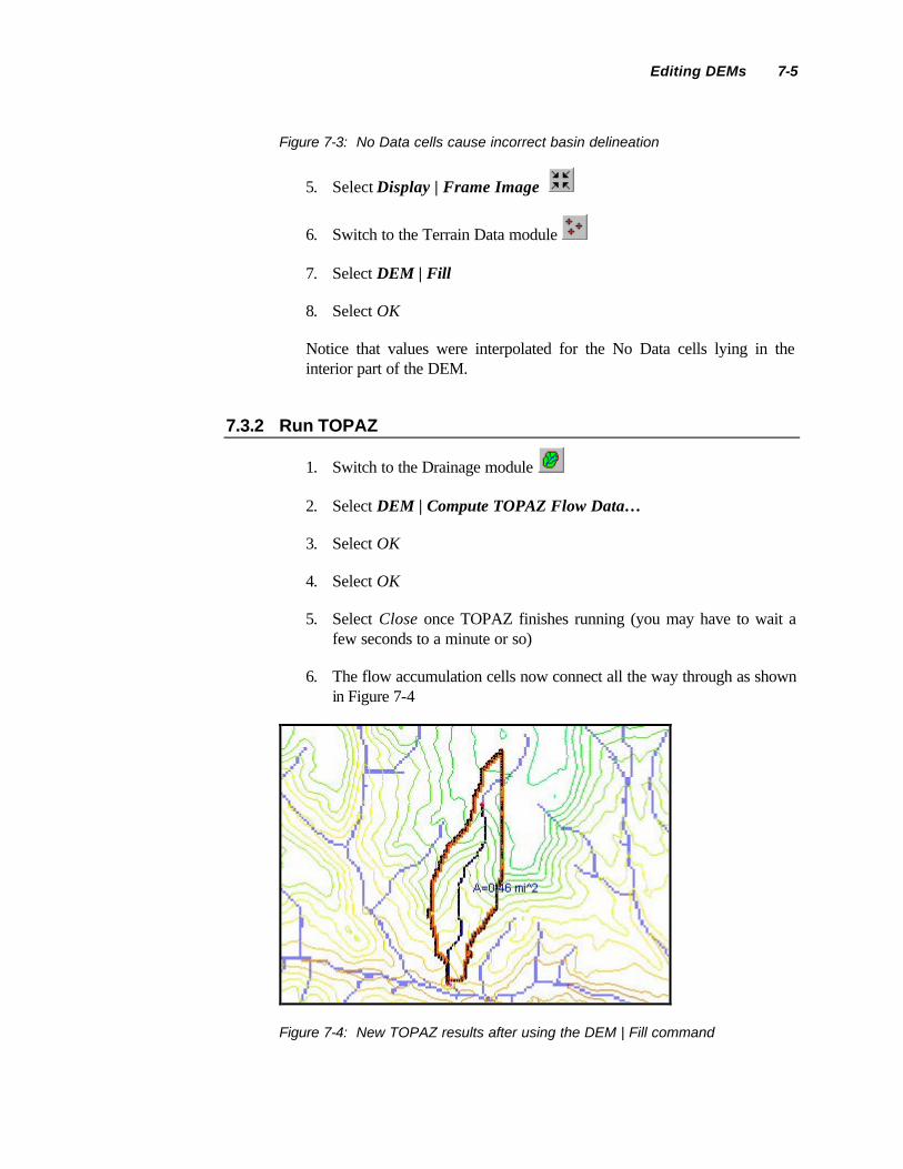
Editing DEMs 7-5
Figure 7-3: No Data cells cause incorrect basin delineation
5. Select Display | Frame Image
6. Switch to the Terrain Data module
7. Select DEM | Fill
8. Select OK
Notice that values were interpolated for the No Data cells lying in the interior part of the DEM.
7.3.2 Run TOPAZ
1. Switch to the Drainage module
2. Select DEM | Compute TOPAZ Flow Data…
3. Select OK
4. Select OK
5. Select Close once TOPAZ finishes running (you may have to wait a few seconds to a minute or so)
6. The flow accumulation cells now connect all the way through as shown in Figure 7-4
Figure 7-4: New TOPAZ results after using the DEM | Fill command

7-6 WMS Tutorials
7.3.3 Basin Delineation
1. Select DEM | Delineate Basins Wizard
2. If prompted, select OK to delete all existing feature data and recreate it using the new basin delineation
3. Select OK
4. Select OK
Figure 7-5 shows the corrected basin delineation.
Figure 7-5: Final basin delineation
7.4 Editing Flow Directions
Flow directions can be inaccurate due to imprecision in the DEM. The flow direction in each DEM cell can be manually edited in order to improve accuracy in basin delineation.
7.4.1 Open DEM
1. Select File | New

Editing DEMs 7-7
2. Select OK
3. Select File | Open…
4. Open “trailmount.dem”
5. Select OK
7.4.2 Open Image
1. Select File | Open…
2. Open “trailmountain.TIF”
3. Zoom in to the area in the rectangle of the DEM as shown in Figure 7-6
Figure 7-6: Zoom in to rectangle
7.4.3 Run TOPAZ
1. Switch to the Drainage module
2. Select DEM | Compute TOPAZ Flow Data…

7-8 WMS Tutorials
3. Select OK
4. Select OK
5. Select Close once TOPAZ finishes running (you may have to wait a few seconds to a minute or so)
Notice that the flow accumulations show a stream that differs from the stream shown in the background image in Figure 7-7.
Figure 7-7: Stream path differences
7.4.4 Edit Flow Directions
Correct the flow directions for each of the numbered DEM cells in Figure 7-8.

Editing DEMs 7-9
Figure 7-8: Edit flow directions for the numbered DEM cells
1. Use the Select DEM points tool and double-click on a numbered cell
This will bring up the DEM Point Attributes dialog shown in Figure 7-9.
Figure 7-9: DEM Point Attributes dialog

7-10 WMS Tutorials
2. Change the flow direction according to Table 7-1
Table 7-1: New flow directions
DEM Cell New Flow Direction
1
2
3
4
3. Select OK
4. Toggle the Compute flow accumulations on ONLY after the last flow direction has been edited
5. Select OK
6. Repeat Step 1-5 for all remaining numbered DEM cells in Figure 1-8
It is possible to edit the flow direction for multiple DEM cells at once using the DEM | Point Attributes command in the Map module
7.4.5 Delineate Basin
1. Use the Create outlet point tool to create an outlet point as shown in Figure 7-10

Editing DEMs 7-11
Figure 7-10: Outlet location
2. Select DEM | Delineate Basins Wizard
3. Select OK
4. Select OK
7.5 Editing Elevations to Create Streams
Stream arcs on a DEM are generally created based on flow directions and flow accumulations. DEM elevations do not always represent the channel elevation of a stream, but might actually be the bank elevation. This can cause streams that have unnatural profiles with drastically varying slopes. We will smooth the stream cell profiles to be more representative of a natural sloping channel.
7.5.1 Editing Elevations Using Stream Arcs
1. Switch to the Terrain Data module
2. Select Display | Display Options…
3. Toggle Stream, Flow Accumulation, Color Fill Drainage Basins, and Fill Basin Boundary Only off
4. On the Map tab change the Points/Nodes and Vertices Radius to 2
5. Select OK
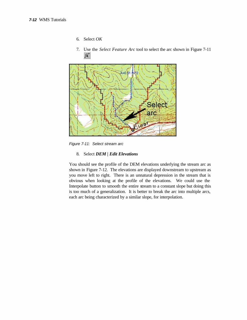
7-12 WMS Tutorials
6. Select OK
7. Use the Select Feature Arc tool to select the arc shown in Figure 7-11
Figure 7-11: Select stream arc
8. Select DEM | Edit Elevations
You should see the profile of the DEM elevations underlying the stream arc as shown in Figure 7-12. The elevations are displayed downstream to upstream as you move left to right. There is an unnatural depression in the stream that is obvious when looking at the profile of the elevations. We could use the Interpolate button to smooth the entire stream to a constant slope but doing this is too much of a generalization. It is better to break the arc into multiple arcs, each arc being characterized by a similar slope, for interpolation.
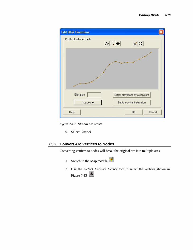
Editing DEMs 7-13
Figure 7-12: Stream arc profile
9. Select Cancel
7.5.2 Convert Arc Vertices to Nodes
Converting vertices to nodes will break the original arc into multiple arcs.
1. Switch to the Map module
2. Use the Select Feature Vertex tool to select the vertices shown in
Figure 7-13

7-14 WMS Tutorials
Figure 7-13: Changing vertices to nodes
3. Select Feature Objects | Vertex <-> Node
7.5.3 Interpolate Elevations
1. Switch to the Terrain Data module
2. Use the Select Feature Arc tool to select the first numbered arc in
Figure 7-14
Figure 7-14: Interpolation arcs
3. Select DEM | Edit Elevations
4. Select the Interpolate button
5. Select OK

Editing DEMs 7-15
6. Repeat the same process for each of the numbered arcs
7.5.4 Convert Arc Nodes to Vertices
Convert the nodes that were created in Section 7.5.2 back to vertices in order to offset the entire arc at once.
1. Switch to the Map module
2. Use the Select Feature Point/Node tool to select the nodes that were
converted from vertices using Figure 7-13
3. Select Feature Objects | Vertex <-> Node
7.5.5 Offset Elevations
Offsetting the elevations of smoothed cells along the stream arc will make a definite stream in the DEM.
1. Switch to the Terrain Data module
2. Use the Select Feature Arc tool to select the original arc shown in
Figure 7-11
3. Select DEM | Edit Elevations
4. Select the Offset elevations by a constant button
5. Enter -2
6. Select OK
7. Select OK
7.5.6 Run TOPAZ
1. Switch to the Drainage module
2. Select DEM | Compute TOPAZ Flow Data…
3. Select OK
4. Select OK
7-16 WMS Tutorials
5. Select Close once TOPAZ finishes running (you may have to wait a few seconds to a minute or so)
7.5.7 Edit Flow Directions
1. Select Display | Display Options…
2. Toggle Flow Accumulation on
3. Select OK
4. Repeat steps in Section 7.4.4 to edit flow directions
7.5.8 Delineate Basin
1. Select DEM | Delineate Basins Wizard
2. If prompted, select OK to delete all existing feature data and recreate it using the new basin delineation
3. Select OK
4. Select OK
7.6 Editing Elevations Using Feature Arcs
DEM cell elevations can be edited to more accurately model the terrain or to reflect man made structures such as roads, dikes or levees, dams, reservoirs, or detention basins. This makes creating a terrain model very versatile and allows you to evaluate a number of different scenarios.
7.6.1 Prepare to Edit Elevations
1. Zoom in around the outlet
2. Switch to the Map module
3. Expand the Map Data folder in the data tree
4. Hide “trailmountain.tif” by toggling its visibility checkbox off
5. Select Display | Contour Options…

Editing DEMs 7-17
6. For the Contour Interval change the Number of contours to 100
7. Select OK
8. Switch to the Terrain Data module
7.6.2 Edit Elevations Using an Generic Arc
1. Use the Create Feature Arc tool to strike an arc as shown in Figure
7-15
Figure 7-15: Feature arc location
2. Select the arc with the Select Feature Arc tool
3. Select DEM | Edit Elevations…
4. Select the Interpolate button
5. Use the Select Point tool to edit the elevation point in the middle of the
profile
6. Select OK when you see the error message about rerunning TOPAZ
The DEM cell represented by the selected profile point is highlighted in the main graphics window

7-18 WMS Tutorials
7. Make sure that the selected profile point corresponds to the DEM cell contains the outlet
8. Drag the selected profile point down approximately to its original elevation, which is represented by the dotted red line in Figure 7-16
Figure 7-16: Editing DEM elevations
9. Select OK and notice the updated contours
We have effectively edited the DEM elevations to represent a small basin/reservoir created by the fill where the road crosses over the drainage point.
7.6.3 Run TOPAZ
1. Switch to the Drainage module
2. Select DEM | Compute TOPAZ Flow Data…
3. Select OK
4. Select OK
Editing DEMs 7-19
5. Select Close once TOPAZ finishes running (you may have to wait a few seconds to a minute or so)
7.6.4 Edit Flow Directions
Repeat the steps in Section 7.4.4 to correct the flow directions again
7.6.5 Delineate Basin
1. Select DEM | Delineate Basins Wizard
2. If prompted, select OK to delete all existing feature data and recreate it using the new basin delineation
3. Select OK
4. Select OK
7.7 Computing a Storage Capacity Curve
A storage capacity curve can be computed based on DEM elevations for any outlet.
1. Use the Select Nodes tool to select the outlet point
2. Select DEM | Create Reservoir
3. Enter 1973 m for the Water Surface Elevation
4. Select OK
The output storage capacity curve will be in English units of acre-ft vs. ft.
7.8 Hydrograph Routing
An input hydrograph can be routed through any reservoir or basin on a DEM by using the storage capacity and elevation discharge curves that are defined in the Detention Basin calculator.
7.8.1 Open an Input Hydrograph
1. Switch to the Hydrologic Modeling module
7-20 WMS Tutorials
2. Use the Select Outlet tool to select the outlet
3. Select Hydrographs | New Hydrographs | From File…
4. Open “hydro.txt”
5. Leave the default settings because this is a tab delimited file. Select Next
6. In the File preview spreadsheet, map the first column type to Time and the second column type to Flow
7. Select Finish
8. Use the Select Hydrograph tool to select the hydrograph
9. Select Display | Open Hydrograph Plot to view the input hydrograph
7.8.2 Elevation Discharge Curve
1. Select Calculators | Detention Basins…
2. Select the Define… button for the Elevation Discharge Curve
3. Choose Discharge structures
4. Select the Add Outlet button
5. Enter 3.14 ft2 for Outlet area
6. Enter 6450.5 ft for Outlet elevation
7. Enter 6448.5 ft for Base elevation
8. Select OK
7.8.3 Compute the Routed Output Hydrograph
1. Select the Compute Outflow Hydrograph button
2. Select OK
3. Select Display | Open Hydrograph Plot to view both the input hydrograph and the routed hydrograph

8 Using Triangulated Irregular Networks
CHAPTER 8
Using Triangulated Irregular Networks
Triangulated Irregular Networks (TINs) are constructed from a scattered set of x y z vertices. They can be used for visualization, as background elevations maps for generating new TINs or DEMs, or to perform basin delineation and drainage analysis. WMS has powerful tools for importing and manipulating this type of terrain data.
8.1 Objectives
The following topics will be covered in this tutorial:
1. Importing survey data
2. Digitizing data
3. Triangulation
4. Automated TIN editing
5. Manual TIN editing
6. Creating a TIN using a conceptual model
7. Converting a TIN to a DEM
8. Exporting data to CAD

8-2 WMS Tutorials
8.2 Importing Survey Data
1. Switch to the Terrain Data module
2. Select File | Open…
3. Open “trailmountain.tif”
4. Select File | Open…
5. Open “surveytm.txt”
6. Leave the default settings. This is a tab delimited file exported from Excel. Select Next
7. For WMS data type choose Survey Data
8. In the File preview spreadsheet, map the first, second, and third column types to X, Y, and Z, respectively.
9. Select Finish
10. Select Display | Display Options…
11. Toggle Unlocked Vertices on
12. Select OK
13. Zoom in around the vertices
8.3 Digitizing Data
1. Select TIN | TIN Options…
2. Choose Digitizing mode
3. Select OK
4. Select the Add Vertices tool from the TIN toolbar (make sure you do not select the Create Feature Point tool from the Feature Objects toolbar—it looks the same as the Add Vertices tool).
5. Enter a Z value of 6800 ft in the edit window at the top of the screen

Using Triangulated Irregular Networks 8-3
6. Digitize the 6800 ft contour by using the background image to add vertices
7. Select TIN | TIN Options…
8. Choose Non-digitizing mode
9. Select OK
8.4 Triangulation
In order to edit the TIN according to the steps in this tutorial we will delete the existing data and read in a TIN file before we triangulate the data.
1. Expand the Terrain Data folder in the Data Tree
2. Right-click on the “surveytm” TIN and select Delete
3. Select File | Open…
4. Open “digitizetm.tin”
5. Zoom in around the vertices
6. Select TIN | Triangle | Triangulate
8.5 Automated TIN Editing
WMS has automated methods of editing TINs so that they provide a representation of terrain that is useful for drainage analysis. These methods include selecting thin boundary triangles, transforming data, and eliminating flat triangles and pits. Thin boundary triangles are an unwanted result of triangulating the data because they do not necessarily represent the terrain. Data transformations are especially useful for converting elevations between feet and meters. Flat triangles need to be eliminated for drainage analysis. Inaccurate basin delineation can result from pits because water flows into the pits rather than to the actual outlet.
8.5.1 Thin Boundary Triangles
1. Select TIN | Triangle | Check Long/Thin Triangles…
2. Choose the Select thin boundary triangles only option

8-4 WMS Tutorials
3. Select OK
4. Use the DELETE button or select Edit | Delete
5. Select OK
8.5.2 Transformations
Run the cursor over the TIN and notice that the z values in the help strip at the bottom of the WMS window are in feet.
1. Select TIN | Vertex | Transform…
2. Enter 0.3048 for the Z Scale value to scale the elevations in feet to meters
3. Toggle the Frame image after transformation option off
4. Select OK
Run the cursor over the TIN and notice that the z values in the help strip have changed to meters.
8.5.3 Flat Triangles
1. Select Display | Display Options…
2. Toggle Flat Triangles on
3. Select OK
4. Select TIN | Triangle | Remove Flat Triangles
8.5.4 Pits
1. Select Display | Display Options…
2. Toggle Pits on
3. Select OK
4. Select TIN | Vertex | Smooth Pits
Some pits may remain even after using this command.

Using Triangulated Irregular Networks 8-5
8.5.5 Delineate Basin
1. Zoom in to the rectangle shown around Pit 1 in Figure 8-1
Figure 8-1: Remaining pits
2. Select TIN Vertices tool . Then, double-click on the TIN vertex shown in Figure 8-2 and change the type from Generic to Drainage outlet

8-6 WMS Tutorials
Figure 8-2: Outlet location
3. Select OK
4. Switch to the Drainage module
5. Select Display | Display Options…
6. Toggle Drainage Basin Boundaries on and change the color to yellow so that they are more visible
7. Select OK
8. Select TIN | Define Basins
9. Use the Flow Path tool to draw flow paths
Figure 8-3: Flow paths
In Figure 8-3 notice that most flow paths flow into Pit 1. This does not allow the flow to make it to the designated outlet point and results in inaccurate basin delineation. Also notice the false dams that have been created from the triangulation. False dams generally occur where a triangle edge lies perpendicular to the stream
8.6 Manual TIN Editing
Manual methods of editing TINs include inserting breaklines, swapping triangle edges, inserting or deleting vertices, and editing vertex elevation and location. Breaklines are useful along streams and ridges by forcing triangle edges to lie along the breakline during triangulation. Swapping triangle edges can eliminate
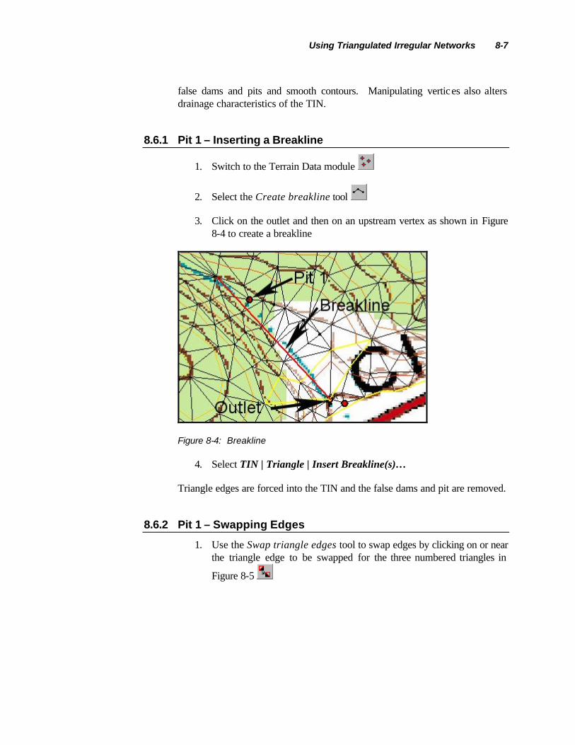
Using Triangulated Irregular Networks 8-7
false dams and pits and smooth contours. Manipulating vertices also alters drainage characteristics of the TIN.
8.6.1 Pit 1 – Inserting a Breakline
1. Switch to the Terrain Data module
2. Select the Create breakline tool
3. Click on the outlet and then on an upstream vertex as shown in Figure 8-4 to create a breakline
Figure 8-4: Breakline
4. Select TIN | Triangle | Insert Breakline(s)…
Triangle edges are forced into the TIN and the false dams and pit are removed.
8.6.2 Pit 1 – Swapping Edges
1. Use the Swap triangle edges tool to swap edges by clicking on or near the triangle edge to be swapped for the three numbered triangles in
Figure 8-5

8-8 WMS Tutorials
Figure 8-5: Jagged contours
Figure 8-6 shows the smooth contours after swapping edges.
Figure 8-6: Contours after swapping edges
2. Zoom out so that you can see the entire TIN
3. Switch to the Drainage module
4. Select TIN | Define Basins
8.6.3 Pit 2 – Inserting a Breakline
1. Zoom in on Pit 2 as shown in Figure 8-7

Using Triangulated Irregular Networks 8-9
Figure 8-7: Pit 2
2. Switch to the Terrain Data module
5. Select the Create breakline tool
6. Create a breakline as shown in Figure 8-8
Figure 8-8: Pit 2 breakline
7. Select TIN | Triangle | Insert Breakline(s)…
3. Zoom out so that you can see the entire TIN

8-10 WMS Tutorials
4. Switch to the Drainage module
8. Select TIN | Define Basins
8.6.4 Pit 3 – Swapping Edges
1. Zoom in on Pit 3 as shown in Figure 8-9
Figure 8-9: Pit 3
2. Use the Swap triangle edges tool to swap edges by clicking on or near the triangle edge to be swapped for the three numbered triangles in
Figure 8-10 and Figure 8-11

Using Triangulated Irregular Networks 8-11
Figure 8-10: Pit 2 swap edges
Figure 8-11: Pit 2 swap edges
3. Zoom out so that you can see the entire TIN
4. Select TIN | Define Basins
8.6.5 Pit 4 – Swapping Edges
1. Zoom in on Pit 4 as shown in Figure 8-12
Figure 8-12: Pit 4
2. Switch to the Terrain Data module

8-12 WMS Tutorials
3. Use the Swap triangle edges tool to swap edges by clicking on or near
the triangle edge shown in Figure 8-13
Figure 8-13: Pit 4 swap edge
When we swap edge 1, a flat triangle is created. Fixing the flat triangle will remove both the flat triangle and the pit.
4. Select TIN | Triangle | Remove Flat Triangles
8.6.6 Delineate Basin
1. Zoom out so that you can see the entire TIN
2. Switch to the Drainage module
3. Select TIN | Define Basins
4. Select TIN | Refine Boundaries
5. Select TIN | Compute Basin Data…
6. Select OK
8.7 Creating a TIN Using a Conceptual Model
A conceptual model built using feature object data can be used to create a TIN. This is important since an arbitrary triangulation of scattered data points may not produce a TIN that is suitable for drainage analysis (i.e. triangle edges enforced along streams and ridges). If you have a set of scattered data points it may be a good idea to triangulate them and then treat them as a background elevation map for creating a new TIN using a conceptual model.

Using Triangulated Irregular Networks 8-13
8.7.1 Open Files
1. Select File | New
2. Select OK
3. Select File | Open…
4. Open “trailmountain.tif”
5. Select File | Open…
6. Open “digitizetm.tin”
7. Zoom in around the x y z data
8.7.2 Triangulation
1. Switch to the Terrain Data module
2. Select Display | Display Options…
3. Toggle Flat Triangles and Pits off
4. Select OK
5. Select TIN | Triangle | Triangulate
8.7.3 Thin Boundary Triangles
1. Select TIN | Triangle | Check Long/Thin Triangles…
2. Choose the Select thin boundary triangles only option
3. Select OK
4. Use the DELETE button or select Edit | Delete
5. Select OK
8.7.4 Creating Feature Arcs for a Conceptual Model
1. Select Display | Display Options…

8-14 WMS Tutorials
2. On the TIN tab toggle Unlocked Vertices and Triangles off
3. On the TIN Drainage tab toggle Drainage Basin Boundaries off
4. Select OK
5. Switch to the Map module
6. Expand the Map Data folder in the Data Tree if necessary
7. Right-click on the “General” coverage and select Properties…
8. Change the Coverage Type to Drainage
9. Select OK
10. Select the Create Feature Arc tool
11. Select Feature Objects | Attributes…
12. Make sure the current feature arc type is set to Generic and select OK
13. Use the Create Feature Arc tool to create an arc that begins and ends at the outlet and follows along the inside edge of the TIN boundary as shown in Figure 8-14
Figure 8-14: Creating an arc along the TIN boundary
Using Triangulated Irregular Networks 8-15
14. Use the Create Feature Arc tool to create an arc starting at the outlet that follows the stream on the background image as shown in Figure 8-14. Make sure you create the arc from downstream to upstream.
15. Use the Select Feature Arc tool to select the arc along the stream
16. Select Feature Objects | Attributes…
17. Choose a Feature Arc Type of Stream
18. Select OK
19. Use the Select Feature Arc tool to select the arc along the TIN
boundary
20. Select Feature Objects | Build Polygon
8.7.5 Redistribute Vertices
The size of the triangles created during triangulation depends on the spacing between vertices.
1. Select Edit | Select All to select all feature arcs
2. Select Feature Objects | Redistribute…
3. Enter a Spacing of 60
4. Select OK
8.7.6 Create TIN
1. Select Display | Display Options…
2. On the TIN tab toggle Triangles on
3. Select OK
4. Select Feature Objects | Create TIN…
5. Select No
6. Toggle the Display triangulation process option on

8-16 WMS Tutorials
7. Select OK
The existing TIN is replaced with a new TIN that was created using the feature arcs that are part of the conceptual model.
8.7.7 Flat Triangles and Pits
1. Switch to the Terrain Data module
2. Select Display | Display Options…
3. Toggle Flat Triangles and Pits on
4. Select OK
5. Select TIN | Vertex | Smooth Pits
8.7.8 Basin Delineation
1. Switch to the Drainage module
2. Select TIN | Define Basins
3. Select TIN | Refine Boundaries
4. Select TIN | Compute Basin Data…
5. Select OK
8.8 Convert to DEM
1. Switch to the Terrain Data module
2. Select TIN | Conversion | TIN->DEM…
3. Enter a cell width and cell height of 10
4. Select OK
5. Select Yes
6. Switch to the Map module

Using Triangulated Irregular Networks 8-17
7. Expand the Map Data folder in the Data Tree and hide the display of “trailmountain.TIF” by toggling the visibility checkbox off
8. Switch to the Drainage module
9. Zoom in around the DEM contours
10. Select DEM | Compute TOPAZ Flow Data…
11. Select OK
12. Select OK
13. Select Close once TOPAZ finishes running (you may have to wait a few seconds to a minute or so)
14. Select Display | Display Options…
15. On the DEM tab change the Minimum Accumulation For Display to 0.005 mi2
16. Select OK
17. Select the Create Outlet Point tool
18. Create an outlet as shown in Figure 8-15
Figure 8-15: DEM outlet
19. Select DEM | Delineate Basins Wizard

8-18 WMS Tutorials
20. Select OK
21. Select OK
22. A new drainage boundary is created using the DEM data. The basin data for this drainage basin is computed.
8.9 Exporting Data to CAD
Data that is visible on the screen can be converted to CAD data and then saved for use in CAD programs.
1. Switch to the Map module
2. Select CAD | Data -> CAD
In order to view only the newly created CAD data we will hide all other data.
3. Hide the Map Data folder in the Data Tree by toggling its visibility checkbox off
4. Switch to the Terrain Data module and hide the Terrain Data folder in
the Data Tree
5. Select Display | Display Options…
6. On the DEM tab toggle Color Fill Drainage Basins and Fill Basin Boundary Only off
7. Select OK
8. Switch to the Map module
9. Select CAD | Display Options…
10. In the Visibility column toggle the “Drainage_arcs” off
11. Select Apply. Notice the CAD data that disappears when selecting this button.
12. Select Cancel
13. Select File | Save As…
14. For Save as type choose the DWG files (*.dwg) filter

Using Triangulated Irregular Networks 8-19
15. Select Save

9 HEC-1 Interface
CHAPTER 9
HEC-1 Interface
WMS has a graphical interface to HEC-1. Geometric attributes such as areas, lengths, and slopes are computed automatically from the digital watershed. Parameters such as loss rates, base flow, unit hydrograph method, and routing data are entered through a series of interactive dialog boxes. Once the parameters needed to define an HEC-1 model have been entered, an input file with the proper format for HEC-1 can be written automatically. Since only parts of the HEC-1 input file are defined in this tutorial, you are encouraged to explore the different available options of each dialog, being sure to select the given method and values before exiting the dialog.
The US Army Corps of Engineers now supports HMS rather than HEC-1, but the hydrologic calculations for the options within HEC-1 have not changed. Results between the two models will be identical.
9.1 Objectives
As a review you will delineate a watershed from a DEM. You will then develop a simple, single basin model using the delineated watershed to derive many of the parameters. Land use and soil shape files (downloaded from the internet) will be used to develop a SCS curve number (CN) value. After establishing the initial HEC-1 model other variations will be developed, including defining multiple basins with reach routing and including a reservoir with storage routing.

9-2 WMS Tutorials
9.2 Delineating the Watershed
Since the land use, soil type, and DEM data for our watershed all originate in the Geographic coordinate system, we will begin by opening them together and converting them to UTM coordinates. The land use and soil type data were downloaded from the EPA website. The DEM data used for this watershed were previously downloaded from the National Elevation Dataset as was demonstrated in the DEM basics tutorial.
1. Select File | Open…
2. Select NED GRIDFLOAT Header (*.hdr) from the Files of type list of file filters
3. Find and open “67845267.HDR”
4. Select OK
5. When prompted if you want to convert the current coordinates select No
9.2.1 Create Land Use and Soil Coverages
1. Switch to the Map module
2. If it is not expanded yet, expand the Map Data folder in the Data Tree window by clicking on the plus mark next to the folder icon
3. Right click on the Map Data folder at the top of the Data Tree
4. Select New Coverage
5. Change the Coverage type to Land Use
6. Select OK
7. Create a new coverage once again and set its Coverage type to Soil Type
9.2.2 Open the Soils Data
1. Make sure the Soil Type coverage is active in the Data Tree
2. Switch to the GIS module
HEC-1 Interface 9-3
3. Select Data | Add Shapefile Data…
4. Open “statsgo.shp”
5. Expand the GIS Layers folder in the Data Tree
6. Right click on statsgo.shp layer in the Data Tree
7. Select Open Attribute Table
Notice that the table has three fields named AREA, PERIMETER, and MUID
8. Select OK
9.2.3 Join Soils Database File Table to Shapefile Table
1. Right click on statsgo.shp in the Data Tree
2. Select Join Table to Layer…
3. Open “statsgoc.dbf”
4. Ensure that Shapefile Join Field and Table Join Field are both set to MUID
5. Change the Table Data Field to HYDGRP
6. Select OK
7. Right click on statsgo.shp in the Data Tree
8. Select Open Attribute Table
Notice that the HYDGRP field is now a part of the shapefile.
9. Select OK
9.2.4 Convert Soil Shapefile Data to Feature Objects
1. Choose the Select Shapes tool
2. Draw a selection box around the DEM extents
3. Select Mapping | Shapes -> Feature Objects
4. Select Next

9-4 WMS Tutorials
This window shows all of the attribute fields in the soils shape file. Because this file was derived from a standard NRCS statsgo file you will notice that the hydrologic soil groups field is named HYDGRP and so WMS will automatically map this to be the soil type. If the attribute field were named anything other than HYDGRP then you would have to manually map it using the drop down list in the spread sheet.
5. Make sure the HYDGRP field is mapped to the SCS soil type attribute
6. Select Next
7. Select Finish
8. Clear the selected polygons by single-clicking somewhere beyond the extents of the shapefile polygons
9. Hide the statsgo.shp file by toggling off its check box in the Data Tree
9.2.5 Open the Land Use Data
1. Switch to the Map module
2. Select the Land Use coverage in the Data Tree to designate it as the active coverage
3. Switch to the GIS module
4. Select Data | Add Shapefile Data…
5. Open “l_richut.shp”
6. Choose the Select Shapes tool
7. Draw a selection box around the DEM extents
8. Select Mapping | Shapes -> Feature Objects
9. Select Next
10. Make sure the LUCODE field is mapped to the Land use attribute
11. Select Next
12. Select Finish

HEC-1 Interface 9-5
13. Hide the l_richut.shp file by toggling off its check box in the Data Tree
9.2.6 Convert/Set the Coordinate System of the Data
1. Select Edit | Coordinate Conversion…
2. Toggle the Edit project coordinate system option on
3. In the Convert From… tab define the Horizontal System to be Geographic NAD 83 (US)
4. Set the Vertical Units to Meters
5. In the Convert To… tab define the Horizontal System to be UTM NAD 83 (US). Zone 12 will automatically be set.
6. Make sure the Horizontal and Vertical Units are Meters
7. Select OK to convert the data
8. Switch to the Map module
9. Since we won’t be using them until later, hide the Land Use and Soil Type coverages by toggling off their check boxes in the Data Tree
10. Select the Drainage coverage from the Data Tree to make sure it is the active coverage
9.2.7 Delineate the Watershed
1. Select the Drainage module
2. Select the Frame macro
3. Select DEM | Compute Topaz Flow Data…
4. Select OK
5. Select OK in the Units dialog
6. Select Close once TOPAZ finishes running (you may have to wait a few seconds to a minute or so)
7. Select the Zoom tool

9-6 WMS Tutorials
8. Zoom in by dragging a box as illustrated in Figure 9-1
Figure 9-1: Zoom in on the area bounded by the rectangle above
9. Select the Create outlet point tool
10. Create a new outlet point where the tributary you just zoomed in on separates from the main stream as illustrated by the arrow in Figure 9-1. Make certain that the outlet point is on the tributary and not part of the main stream. Also, the outlet needs to be inside one of the flow accumulation (blue) cells. WMS will move the outlet to the nearest flow accumulation cell if you do not click right in one of the flow accumulations cells.
11. Select the Frame macro
12. Select DEM | Delineate Basins Wizard
13. Select OK
14. Select OK
You have now completed the delineation of a single watershed. In order to make the view clearer for defining the hydrologic model you can turn off many of the DEM and other display options.
15. Select the Display Options macro

HEC-1 Interface 9-7
16. On the DEM tab toggle off the display for Watershed, Stream, Flow Accumulation, and DEM Contours
17. On the Map tab toggle off the display of Vertices
18. Select OK
9.3 Single Basin Analysis
The first simulation will be defined for a single basin. You will need to enter the global, or Job Control parameters as well as the rainfall event, loss method, and unit hydrograph method.
9.3.1 Setting Up the Job Control
Most of the parameters required for a HEC-1 model are defined for basins, outlets, and reaches. However, there are many “global” parameters that control the overall simulation and are not specific to any basin or reach in the model. These parameters are defined in the WMS interface using the Job Control dialog.
1. Select the Hydrologic Modeling module
2. HEC-1 should be the default model, but if it is not select it from the drop down list of models found in the Edit Window
3. Select HEC-1 | Job Control…
4. The first three lines are for comments/identification at the top of the HEC-1 input file. The first line already has information indicating that the input file is generated by WMS (you can change this if you want). Enter Clear Creek Tributary Watershed for the second ID line. Enter your name and current date in the third line.
5. Leave the Day, Month, and Field years alone
HEC-1 allows you to enter a date, but almost always you are simulating some kind of hypothetical or design storm and not an actual storm. If you change the simulation date you will need to be careful to make sure the storm date is in synch, but if you leave it alone then there will not be a problem.
6. Enter 5 (minutes) for the Computation time interval, and 300 for the Number of hydrograph ordinates. Leave the starting time at 0.

9-8 WMS Tutorials
A HEC-1 simulation will run for a length of time equal to the time step multiplied by the number of ordinates. If you are simulating a 24-hr storm but only run the simulation for 12 hours you will not capture the full hydrograph. Conversely if you run a 24-hr simulation for 96-hrs you are probably going to have a lot of runoff ordinates equal to 0 at the end. In this case we are running the simulation for 1500 minutes (slightly more than 24 hours) with an ordinate on the hydrograph being computed for every 5 minutes.
7. Set the computation units to English (this should be the default)
Setting the computation units DOES NOT cause any units conversion to take place. You are simply telling HEC-1 that you will provide input units in English units (sq. miles for area, inches for rain, feet/miles for length) and expect results of computation to be in English units (cfs). If you specify Metric then you must insure that input units are metric (sq. kilometers, mm for rain, meters/kilometers for lengh) and results will be in metric (cms).
8. Select OK
For now we will leave the other Job Control settings at their default values.
9.3.2 Setting up the Basin Data Parameters
In the first simulation you will treat the entire watershed as a single basin.
1. Select the Select Basin tool
2. Double-click on the brown basin icon labeled 1B. Double-clicking on a basin or outlet icon always brings up the parameter editor dialog for the current model (in this case HEC-1)
3. Select the Basin Data button
4. Notice that the area has been calculated (in this case in sq. mile s because we are performing calculations in English units)
5. Change the name to CCTrib. HEC-1 will only use the first SIX characters so do not use names longer than six characters for basins or outlets.
6. Select OK
7. Select the Precipitation button
8. Select the Basin Average option
9. Enter 1.8 (inches) for the Average precipitation depth

HEC-1 Interface 9-9
10. Select the Define Series button
In order to simulate a rainfall event you must enter both a rainfall depth and a temporal distribution. The SCS uses standard time distributions for different areas of the U.S. These series have been created and stored in a file that you can import. You could also define your own series according to an actual storm, or a design storm from a regulating agency.
1. Select the Import button
2. Find and open the file named “scstabs.xys”. You may need to change the Files of type filter to All Files (*.*) in order to see the file.
3. In the Selected Curve drop down list select the typeII-24hour curve
4. Select OK
5. Select OK
6. Select the Loss Method button
7. Enter a Curve Number (CRVNBR field) of 70. We will compute a CN value from actual land use and soil files later.
8. Select OK
9. Select the Unit Hydrograph Method button
10. Make sure the SCS dimensionless option is chosen (it is the default)
11. Select the Compute Parameters - Basin Data button
12. Set the Computation Type to Compute Lag Time (the default)
13. Set the Method drop down list to SCS Method (near the bottom of the list)
14. Select OK to update the computed lag time for the SCS dimensionless method
15. Select OK
16. Select Done
You now have all of the parameters set to run a single basin analysis.

9-10 WMS Tutorials
9.3.3 Running HEC-1
Whenever you run a HEC-1 simulation WMS will first save a standard HEC-1 input file. You will also be prompted for the name of an output file and a solutions file. The output file is the standard text output file generated by HEC-1 and the solution file is a plot file that contains the hydrographs formatted in a way that makes it easy for WMS to read and plot (it is actually the HEC-1 TAPE22 file).
1. Select HEC-1 | Run Simulation…
2. Change the text in the Prefix for all files field to be CCTrib
3. Select the Update All Prefixes button
4. Select OK
5. Select Close once HEC-1 finishes running (you may have to wait a few seconds to a minute or so)
The solutions will automatically be read in and you should see a small hydrograph plot up and to the right of the Basin icon (now labeled as CCTrib).
1. Double-click on the hydrograph icon.
A plot window will appear with the hydrograph. You will see that the hydrograph suddenly stops at 1500 minutes (the duration of the simulation as established in the Job Control dialog), but the simulation obviously has not run to completion.
1. Close the plot window by selecting the X in the upper right corner of the window
2. Select Hydrographs | Delete All
3. Select HEC-1 | Job Control…
4. Set the Number of hydrograph ordinates to be 400
5. Select OK
6. Select HEC-1 | Run Simulation…
7. Select OK (you can le t it overwrite the other files)
8. Select Close once HEC-1 finishes running (you may have to wait a few seconds to a minute or so)

HEC-1 Interface 9-11
9. Double-click on the hydrograph icon
You now have a completed HEC-1 simulation for a single basin and the resulting hydrograph should look something like the solution shown in Figure 9-2.
0
50
100
150
200
250
300
350
400
450
500
0 250 500 750 1000 1250 1500 1750 2000
Flow vs. TimePEAK: 488.18; TIME OF PEAK: 890min.; VOLUME: 12598963.35
Flo
w (
cfs)
Time
Index 1, CCTrib
Figure 9-2: Solution hydrograph for HEC-1 simulation
1. Close the hydrograph window by selecting the X in the upper right of the window
9.4 Computing the CN Using Land Use and Soils Data
In the initial simulation you just estimated a CN, but with access to the internet it is simple to compute a composite CN based on digital land use and soils files. This was demonstrated in more detail in the Advanced Feature Objects tutorial, but you will go through the steps here as a review.
9.4.1 Computing a Composite CN
In addition to the digital land use and soils file that overlap the watershed you must have a table defined that identifies CN values for each of the four different hydrologic soil groups (A, B, C, D). This is described in detail at the gsda website (http://emrl.byu.edu/gsda), and in the advanced feature objects tutorial. For this tutorial you will read in an existing file (you can examine it in a text editor if you wish) and compute the CN numbers.

9-12 WMS Tutorials
1. Select the Hydrologic Modeling module
2. Select Calculators | Compute GIS Attributes…
3. Select the Import button to load the mapping table
4. Select OK to overwrite the current definition
5. Find and open the file named “scsland.tbl”
6. Select OK to compute the CN from the land use and soils layers
You should find that CN computed from the land use and soils digital data is about 72 or 73. While there is still some “judgment” required in setting up the mapping table, there is a lot more justification for this value than the one previously estimated.
9.4.2 Run HEC-1
You can now run another simulation to compare the results with the modified CN value.
1. Select HEC-1 | Run Simulation…
2. Select OK (it is fine to overwrite the existing files, but you can change the file names if you want)
3. Select Close once HEC-1 finishes running (you may have to wait a few seconds to a minute or so)
4. Double-click on the hydrograph icon to plot both the old and the new hydrograph in a plot window
With the increased CN value you should see that the resulting hydrograph peaks higher (more runoff). The peak should be about 600 cfs rather than the 500 cfs that was generated with a CN value of 70.
1. Close the hydrograph window by selecting the X in the upper right corner of the window.
2. Select Hydrographs | Delete All

HEC-1 Interface 9-13
9.5 Adding Sub-basins and Routing
You will now subdivide the watershed into two upper basins and one lower basin and define routing for the reaches that connect the upper basins to the watershed outlet.
9.5.1 Delineating the sub-basin
1. Select the Drainage module
2. Select the Zoom tool
3. Create a zoom box around the region identified by a box in Figure 9-3
Figure 9-3: Zoom in on the area indicated by the rectangle.
1. Select Display | Display Options…
2. On the Map tab toggle on Vertices
3. Select OK
4. Select the Select Vertex tool
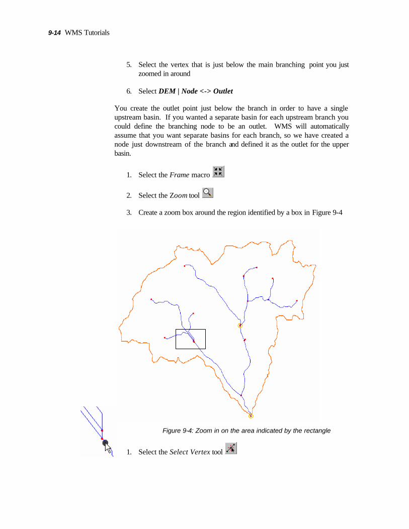
9-14 WMS Tutorials
5. Select the vertex that is just below the main branching point you just zoomed in around
6. Select DEM | Node <-> Outlet
You create the outlet point just below the branch in order to have a single upstream basin. If you wanted a separate basin for each upstream branch you could define the branching node to be an outlet. WMS will automatically assume that you want separate basins for each branch, so we have created a node just downstream of the branch and defined it as the outlet for the upper basin.
1. Select the Frame macro
2. Select the Zoom tool
3. Create a zoom box around the region identified by a box in Figure 9-4
Figure 9-4: Zoom in on the area indicated by the rectangle
1. Select the Select Vertex tool

HEC-1 Interface 9-15
2. Select the vertex that is just below the feature node where the streams branch
3. Select DEM | Node <-> Outlet
4. Select the Frame macro
5. Select DEM | Delineate Basins Wizard
6. Select OK to delete and recreate feature data
7. Select OK
8. Select OK
9.5.2 Updating the Basin Parameters
You will have to recompute the CN values and define precipitation and lag time for the basins.
1. Select the Hydrologic Modeling module
2. Select Calculators | Compute GIS Attributes…
3. Select OK and the CN values will be updated for all basins (they are actually very similar in this case because of the dominant soil polygon that covers the watershed)
4. Select the Select Basin tool
5. Double-click on the upper right basin icon to bring up the Edit HEC-1 Parameters dialog
6. Select the Basin Data button
7. Change the Name to Right
8. Select OK
9. Move the Edit HEC-1 Parameters dialog out of the way, if necessary, and click on the upper left basin icon to edit parameters for the upper left basin
10. Select the Basin Data button
11. Change the Name to Left

9-16 WMS Tutorials
12. Select OK
13. Move the Edit HEC-1 Parameters dialog out of the way, if necessary, and click on the lower basin icon to edit parameters for the lower basin
14. Select the Basin Data button
15. Change the Name to CCTrib
16. Select OK
17. Select Done
18. Select Edit | Select All to select all basins
19. Select HEC-1 | Edit Parameters… to edit parameters for all basins at once
20. Select the Precipitation button
21. Select the Basin Average option
22. Set the Average Precipitation to be 1.8
23. Select the Define Series button
24. Choose the typeII-24hour curve in the Selected Curve drop down list
25. Select OK
26. Select OK
27. Select the Unit Hydrograph Method button
28. Make sure the SCS dimensionless option is chosen (it is the default)
29. Select the Compute Parameters – Basin Data button
30. Select CCTrib in the Basin window so that it is highlighted
31. Select the Method to be SCS Method (near the bottom of the list)
32. Select Left in the Basin window so that it is highlighted
33. Select the Method to be SCS Method (near the bottom of the list)
34. Select Right in the Basin window so that it is highlighted
35. Select the Method to be SCS Method (near the bottom of the list)

HEC-1 Interface 9-17
36. Select OK
37. Select OK
38. Select Done
9.5.3 Setting up the Routing Parameters
If you were to run HEC-1 now (you can if you want) you would see that the hydrographs from the upper basins would be combined with the lower basin hydrograph at the watershed outlet without any lag or attenuation because you haven’t yet set the routing parameters. You will now define a routing method, which will instruct HEC-1 to compute lag and attenuation on the upper basin hydrographs before adding them to the lower hydrograph.
Routing for a reach is always defined at the upstream outlet of the reach in WMS.
1. Select the Select Outlet tool
2. Double-click on the outlet (the yellow circle icon) of the upper right basin
3. Select the Routing Data button
4. Select the Muskingum-Cunge method for routing
5. Set the width (WD) field to be 5 (five feet wide)
6. Set the side slope value (Z) to be 1 (1:1 side slope)
7. Set the Manning’s roughness (N) to be 0.05 (this is kind of rough but we want to exaggerate the routing effects for this tutorial)
8. Select OK
9. Select Done
10. Double-click on the outlet of the upper left basin
11. Select the Routing Data button
12. Select the Muskingum-Cunge method for routing
13. Set the width (WD) field to be 5

9-18 WMS Tutorials
14. Set the side slope value (Z) to be 1
15. Set the Manning’s roughness (N) to be 0.05
16. Select OK
17. Select Done
9.5.4 Running HEC-1
You now have everything defined to run a three basin HEC-1 analysis that includes routing the upper basins through the reaches connecting them to the watershed outlet.
1. Select HEC-1 | Run Simulation…
2. Change the name in the Prefix for all files field to Routing
3. Select the Update All Prefixes button
4. Select OK
5. Select Close once HEC-1 finishes running (you may have to wait a few seconds to a minute or so)
6. While holding the <SHIFT> key down select all of the hydrograph icons, double-clicking on the last one so that all hydrographs are drawn in the same plot window
7. Close the plot window by selecting the X in the upper right corner
9.6 Modeling a Reservoir in HEC-1
There is an existing small reservoir at the outlet of the upper left basin. It has a storage capacity of 1000 ac-ft at the spillway level and 1540 ac-ft at the dam crest.
9.6.1 Defining a Reservoir in Combination with Routing
One of the routing methods available in HEC-1 is Storage routing, which can be used to define reservoir routing. However, in this case we are already using Muskingum-Cunge routing to move the hydrograph through the reach connecting the upper left basin to the watershed outlet so we must define the outlet as a reservoir so that we can route the hydrograph through the reservoir before routing it downstream.

HEC-1 Interface 9-19
1. Select the Select Outlet tool
2. Select the outlet of the upper left basin
3. Select Tree | Add Reservoir
9.6.2 Setting up the Reservoir Routing Parameters
In order to define reservoir routing with HEC-1 you must define elevation vs. storage (storage capacity curve) and elevation vs. discharge rating curves. You can enter values directly, or enter hydraulic structures and compute the values, but in this tutorial you will enter the values directly. You will use the same elevation values for both curves (this is common, but not a requirement in HEC-1).
For this example we want to have no outflow until the elevation in the reservoir reaches the spillway. Since HEC-1 linear interpolates between consecutive points on the elevation-discharge and elevation-volume curves we will “trick” it by entering two points on the curves at essentially the same elevation (6821.99 and 6822) with the first having no outflow and the second having the discharge over the spillway (640 cfs) as defined for this dam.
1. Double-click on the reservoir outlet point (it is now represented as a triangle since you have defined a reservoir at this location)
2. Select the Reservoir Data button
3. Change the Reservoir name to Tcreek
4. Set the Type of storage routing to Reservoir
5. Select the Define button to the right of the reservoir option
6. On the right side of this dialog you will define the Volume or storage capacity data. Choose the Known Volume option.
7. Toggle on the check boxes for SV (Volumes) and SE (Elevations)
8. Select the Define button to the right of the SV option
You will define separate XY series for Volumes, Elevations, and Discharges using the WMS XY Series editor.
1. Select New
2. Change the name of the new curve to Volume

9-20 WMS Tutorials
3. In the first seven edit fields enter the values 0, 200, 410, 650, 1000, 1000, 1540 (acre-ft of volume)
4. Select the 8th through 20th edit fields and select the <DELETE> key so that the values are blank rather than zero. You can select them all at once (the way you do in a spreadsheet since this dialog behaves like a spreadsheet) by clicking in the top and while holding the mouse button down dragging to the last, or you can select one at a time.
Figure 9-5: The XY Series editor for inputting volumes.
1. Select OK
2. Select the Define button to the right of the SE option
3. Select New
4. Change the name of the new curve to Elevation
5. In the first seven entry fields enter the following values: 6803, 6808, 6813, 6818, 6821.99, 6822, 6825 (feet of elevation)
6. Set the 8th through 20th fields blank instead of zero as with the volume series
7. Select OK
8. On the left side of this dialog you will define the Outflow or elevation - discharge data. Choose the Known Outflow option.
9. Toggle on the check boxes for SQ (Discharges) and SE (Elevations)
10. Select the Define button to the right of the SQ option

HEC-1 Interface 9-21
11. Select New
12. Change the name of the new curve to Discharge
13. In the first seven entry fields enter the following values: 0, 0, 0, 0, 640, 640, 7000 (cubic feet per second of flow). There is no outflow until the water reaches the spillway.
14. Set the 8th through 20th fields blank instead of zero as with the volume series
15. Select OK
16. Select the Define button to the right of the SE option
This time rather than creating a new curve you will select the elevation curve previously defined for the storage capacity curve.
1. Select the Elevation curve from the Selected Curve drop down list
2. Select OK
If you would like you may plot either the elevation-discharge or the elevation-volume curves by selecting the Plot SQ-SE or Plot SV-SE buttons. This will bring the curve into a plot window that you can export, print, or control the same way you can a hydrograph or any other plot in a plot window.
1. Select OK
The last thing you need to input to define reservoir routing is the initial conditions of the reservoir. The initial condition can be defined as an elevation, a discharge, or a volume (with the data you just entered HEC-1 can determine the initial condition of the other two based on the one you enter). For this example we will set the initial condition to an elevation four feet below the top of the spillway (the spillway corresponds to elevation 6822).
1. Under the Initial Condition Type select the ELEV option
2. Set the RSVRIC (reservoir initial condition) to be 6818
3. Select OK
4. Select Done
9.6.3 Running HEC-1
You are now ready to save and run the HEC-1 file with the defined reservoir.

9-22 WMS Tutorials
1. Select HEC-1 | Run Simulation…
2. Change the name in the Prefix for all files field to Reservoir
3. Select the Update all prefixes button
4. Select OK
5. Select Close once HEC-1 finishes running (you may have to wait a few seconds to a minute or so)
6. After HEC-1 runs you can open any (or multiple within the same plot window by holding down the <SHIFT> key to multi-select) of the hydrographs by double-clicking on the corresponding icon.
7. Close all plot windows before moving on
9.7 Reviewing Output
It should be emphasized here that while WMS makes it easy to set up a HEC-1 model and compute a result, it is not a substitute for understanding the basic theory and equations used in HEC-1. You are encouraged to read the HEC-1 manual found in the documents directory distributed with WMS and other texts on hydrologic modeling. You are also encouraged to review the HEC-1 output file that is generated with each simulation in order to glean more understanding about how your model is working.
1. Select File | Edit File…
2. Find and open the file named “reservoir.out”
3. Select OK to open the file with Notepad
4. Scroll through this file and examine what information HEC-1 saves to the output file. If you have errors running HEC-1 simulations you may often find the answer to the problem within the *.out output file.
9.8 Conclusion
This concludes the tutorial on defining HEC-1 files and displaying hydrographs. The concepts learned include the following:
• Entering job control parameters

HEC-1 Interface 9-23
• Defining basin parameters such as loss rates, precipitation, and hydrograph methodology for a single watershed or a multiple basin analysis
• Defining routing parameters
• Routing a hydrograph through a reservoir
• Saving HEC-1 input files
• Reading hydrograph results


10 Rational Method Interface
CHAPTER 10
Rational Method Interface
The Rational Method is one of the simplest and best known methods routinely applied in urban hydrology. Peak flows are computed from the simple equation:
kCiAQ =
where:
Q - Peak flow
k - conversion factor
C - Runoff coefficient
i - Rainfall intensity
A - Area
In this tutorial you will learn how to solve problems using a digital terrain model and the Rational Method.
10.1 Reading in Terrain Data
The terrain model used in this tutorial is a TIN for a small portion of a city. The elevation data was obtained by digitizing a contour map.
1. Select File | Open…
2. Find and open “afrational.tin”.

10-2 WMS Tutorials
3. Select the Drainage module .
4. Select TIN | Compute Basin Data.
5. The Model Units should be feet. Set the Parameter Units to be Acres for Basin Areas and Feet for Distances.
6. Select OK.
10.2 Running a Rational Method Simulation
The areas computed from the TIN can now be used in setting up a Rational Method simulation of the urban development. Each of the outlet points represents an inlet to a storm drain.
1. Select the Hydrologic Modeling module .
2. Select Rational to be the current model from the drop down list of models in the Edit Window.
3. Double-click the basin icon for the basin labeled “Upper” in Figure 10-1.
The Rational Method dialog should appear. While this dialog is up you can continue to interact with the menus, tools, and windows of WMS. As you select different basins, the current parameters will be updated in the dialog.
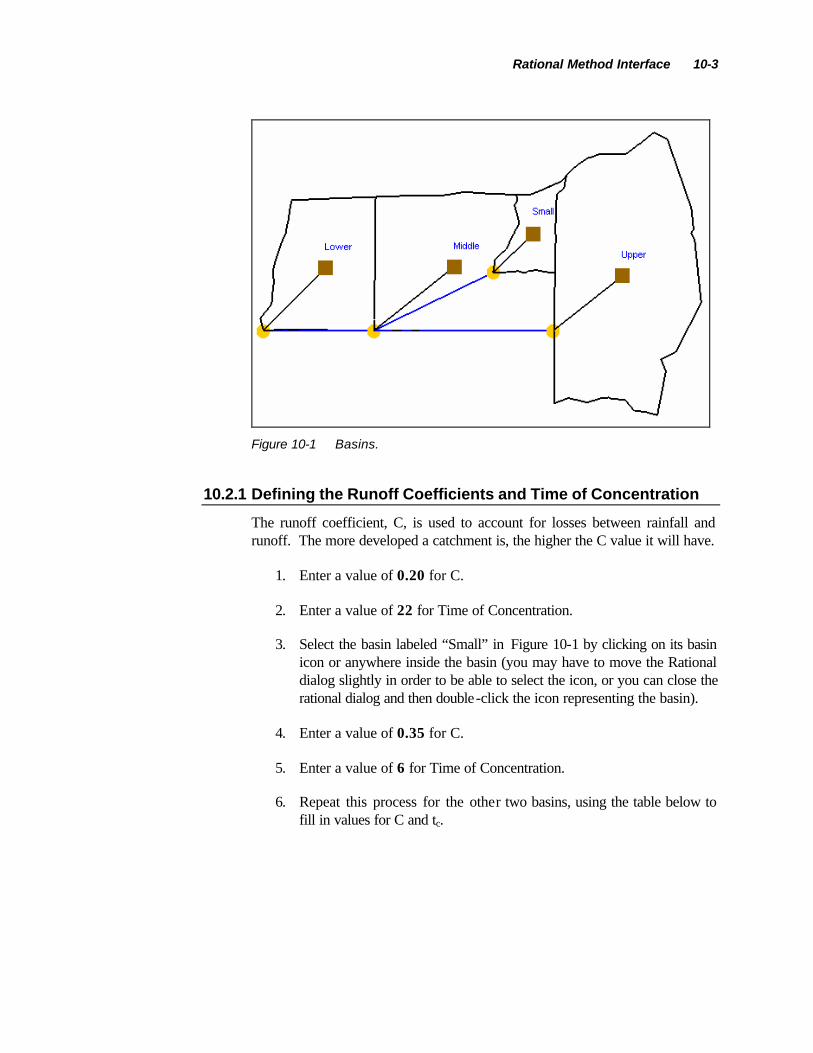
Rational Method Interface 10-3
Figure 10-1 Basins.
10.2.1 Defining the Runoff Coefficients and Time of Concentration
The runoff coefficient, C, is used to account for losses between rainfall and runoff. The more developed a catchment is, the higher the C value it will have.
1. Enter a value of 0.20 for C.
2. Enter a value of 22 for Time of Concentration.
3. Select the basin labeled “Small” in Figure 10-1 by clicking on its basin icon or anywhere inside the basin (you may have to move the Rational dialog slightly in order to be able to select the icon, or you can close the rational dialog and then double-click the icon representing the basin).
4. Enter a value of 0.35 for C.
5. Enter a value of 6 for Time of Concentration.
6. Repeat this process for the other two basins, using the table below to fill in values for C and tc.

10-4 WMS Tutorials
Basin Name Runoff Coefficient C Time of Concentration tc
Upper .2 22 Small .35 6 Middle .4 18 Lower .4 11
7. When you are finished entering the parameters choose Done on the Rational Method dialog.
A runoff coefficient coverage could be used to automatically map C values and basin data or a time computation coverage could be employed to determine Tc values, but they can also be computed/estimated separately and entered as demonstrated here.
10.2.2 Defining the Rainfall Intensity (i)
As part of the WMS interface to the Rational Method you can compute IDF curves using either HYDRO-35, NOAA, or user defined data. For this tutorial we will use HYDRO-35 data and a recurrence interval of 10 years.
1. Double-click the icon for the “Upper” catchment.
2. Select the IDF Curves… button from the Basin section of the Rational Method dialog.
3. Make sure the HYDRO-35 Data (Eastern US) radio group button is selected and select the Define Data button.
4. Enter the following values to define IDF curves using HYDRO-35
Time (min) Depth (in)
2 yr. 5 min. .47 2 yr. 15 min. .97 2 yr. 60 min 1.72 100 yr. 5 min. .81 100 yr. 15 min. 1.75 100 yr. 60 min. 3.60
1. Select the OK button after correctly entering the rainfall values.
The IDF curves for the 2, 5, 10, 25, 50, and 100 year recurrence intervals will be drawn, and values listed for selected times given in the windows on the right of the IDF Computation dialog.
1. From the text window in the upper right hand part of the dialog click on the line of data for the 10-yr recurrence interval as shown in Figure 10-2.

Rational Method Interface 10-5
Figure 10-2 IDF Computation Dialog with the 10-yr Recurrence Interval
Selected.
The rainfall intensity is determined from the selected interval by using the previously defined value for time of concentration.
1. Compute i by selecting the Intensity button.
2. Select the Done button. The value of i computed using the IDF-Computation dialog will be placed in the edit field for this basin.
3. Note also that the input for this basin is complete and a value for runoff Q has been computed. A summary of the rational equation and results is in the upper right window of the dialog.
The HYDRO-35 data only needs to be entered once (unless different data is to be used for different basins), so the rainfall intensity for the remaining basins can be defined using the following steps.
1. Select the icon for “Small”.
2. Select the IDF Curves button.
3. Select the line of text for the 10-yr recurrence interval.
4. Select the Intensity button.

10-6 WMS Tutorials
5. Select Done.
6. Repeat these steps for the Middle and Lower basins.
7. When you are finished entering the parameters choose Done on the Rational Method dialog.
10.2.3 Defining Hydrographs
As the data entry for each basin is completed, a peak flow (Q) is computed and listed in the text display window. The Rational Method equation does not produce a hydrograph. However, several different unit-dimensionless hydrographs can be used to distribute the peak flow through time to create a runoff hydrograph.
1. Double-click the basin labeled “Upper” in Figure 10-1.
2. Select the Define Hydrographs… button.
3. Select the Rational method hydrograph from the drop down list.
4. Select Done to compute the hydrograph.
5. Select Done for the Rational Method dialog.
6. Double-click on the small hydrograph box to the upper right of the basin icon to open up a plot window with the hydrograph.
You should see the hydrograph displayed in a plot window as shown in Figure 10-3.

Rational Method Interface 10-7
Figure 10-3 Rational Method Hydrograph for a Basin.
1. When you are finished viewing the hydrograph close the plot window by selecting the X in the upper right corner of the window.
10.2.4 Defining Rainfall Intensities at the Outlet to Compute Runoff Hydrographs
WMS can determine composite rational method parameters at the outlet for computing hydrographs. The time of concentration at an outlet point is defined as the longest flow time from upstream basins (times of concentration) combined with any lag times from channels. The area is the cumulative upstream area, and the runoff coefficient is determined as an area weighted value from the upstream basins. With the time of concentration at the outlet defined you will need to determine the appropriate rainfall intensity. In order for WMS to compute peak flows and hydrographs at outlets you will need to define the travel time between outlets and the intensities for the time of concentration at each outlet.
1. Select the Select Outlet tool .
2. Double-click the outlet icon of Upper as shown in Figure 10-1 (be sure to select the circular outlet icon and not the square basin icon).
You will note in the Outlet portion of the Rational Method dialog that information upstream from this outlet has been aggregated (in the case though there is just one basin upstream). The longest flow time is listed for the time of

10-8 WMS Tutorials
concentration, a cumulative area, and a weighted C value as shown in Figure 10-4.
Figure 10-4 Outlet Information for a Rational Method Simulation..
1. Enter a value of 5 minutes for the Routing lag time.
2. Select the IDF Curves… button.
3. Select the line of text for the 10-yr-recurrence interval.
4. Select Done.
5. Select the outlet icon of Small.
6. Enter a value of 3 minutes for the Routing lag time.
7. Select the IDF Curves… button.
8. Select the line of text for the 10-yr-recurrence interval.
9. Select Done.
10. Select the next downstream outlet (the outlet icon of Middle).
Note that for this outlet the upstream areas are summed, the C valued weighted, and the longest travel path computed from the upstream basin Tc’s and travel times between outlets determined.
1. Enter a value of 4 minutes for the Routing lag time.
2. Select the IDF Curves… button.
3. Select the line of text for the 10-yr-recurrence interval.
4. Select Done.

Rational Method Interface 10-9
The last or bottom-most outlet does not need to have a Routing lag time defined since the hydrograph accumulations will occur at this point, but you will still need to define the rainfall intensity.
1. Select the bottom-most outlet point.
2. Select the IDF Curves… button.
3. Select the line of text for the 10-yr-recurrence interval.
4. Select Done.
5. Select the Define Hydrographs… button.
6. Choose the Traditional method.
7. Choose the Rational Method hydrograph option.
8. Select Done.
9. Select Done in the Rational Method dialog also.
10. Double-click on the hydrograph icon for the most downstream outlet.
11. Close the hydrograph plot window when you are done viewing by selecting the X in the upper right corner of the window.
10.2.5 Combining Runoff from Multiple Basins
Besides the traditional method of computing peak flows and hydrographs for multiple sub-basins within a watershed, WMS will also allow you to lag hydrographs computed for basins and add at outlets in order to produce downstream peak flows and hydrographs.
1. Double-click on the downstream-most outlet point (outlet of the Lower basin).
2. Select the Define Hydrographs… button.
3. Choose the Route by summing method.
4. Choose the Rational method hydrograph option.
5. Select Done.
6. Select Done.
7. Double-click the hydrograph icon for the bottom-most outlet.

10-10 WMS Tutorials
You can now see the difference between these two methods as both hydrographs are plotted in the window.
1. Close the hydrograph plot window when you are done viewing by selecting the X in the upper right corner of the window.
10.3 Adding a Detention Basin
If you compute runoff using the route by summing method then you can route hydrographs through detention basin structures defined at any of the outlet locations.
1. Double-click the outlet that defines the Small catchment in Figure 10-1.
2. Select the Define Reservoir button.
You will now define a hypothetical detention basin for the Small catchment from approximate geometric parameters. WMS can compute a storage capacity curve for a rectangular basin. You could also enter a pre-computed storage capacity curve.
1. Select the Define… button in the Storage Capacity box.
2. Select the Known Geometry option.
3. Enter 200 feet for Length.
4. Enter 300 feet for Width
5. Enter a Depth of 30 feet.
6. Enter a Side slope of 2
7. Leave the Base elevation at 0.0 (It will be assumed on-grade at the outlet location).
8. Select OK.
You will now define a standpipe and spillway (weir) for outlet structures and WMS will compute the elevation-discharge relationship automatically. In addition to standpipes and weirs you can define low-level outlets, or you can enter a pre-computed elevation-discharge relationship.
1. Select the Define… button in the Elevation Discharge box.
2. Select the Discharge Structures option.

Rational Method Interface 10-11
3. Select the Add Standpipe button.
4. Set the Pipe diameter to 4 feet.
5. Set the Standpipe elevation to 15 feet.
6. Select the Add Weir button.
7. Set the Weir width to 20 feet.
8. Set the Weir elevation to 25 feet.
9. Select OK.
10. Select OK.
You have now defined a detention facility that has a standpipe and a spillway for control structures. The incoming hydrograph to this outlet point will be routed through the detention facility before being routed downstream and combined with the hydrographs of other basins.
1. Select the bottom-most outlet point.
2. Select the Define Hydrographs… button.
3. Choose the Route by summing method.
4. Choose the Universal hydrograph method.
5. Select Done.
6. Select Done.
7. Double-click on the hydrograph box for the bottom-most outlet.
10.4 Conclusions
In this tutorial you have learned some of the options available for using the rational method in WMS. You will want to continue experimenting with the different options so that you can become familiar with all the capabilities in WMS for doing Rational Method simulations.


11 National Flood Frequency Program (NFF) Interface
CHAPTER 11
National Flood Frequency Program (NFF) Interface
The National Flood Frequency program, developed by the USGS, provides a quick and easy way of estimating peak flows for ungaged watersheds. This data can be used in the design of culverts, flood-control structures, and flood-plain management. It utilizes regression equations that have been developed for each state. Most regression equations are functions of parameters such as area, slope, and runoff distance that are automatically computed by WMS when delineating a watershed.
In this tutorial you will compute peak flows for a watershed in Florida. An important part of runoff prediction in this region is the percent coverage of water bodies and so this is reflected in many of Florida’s equation. There is not a direct calculation method available in WMS to determine the percentage of water-covered area in a watershed, but you will learn how you can use GIS overlay tools to compute percentages for any land use type within a watershed. This same method could be applied for equations in other states that require a percentage of water body coverage, or forested areas, or some other land use or soil formation that can be obtained from a shapefile or other GIS layer useable by WMS.
11.1 Opening the Drainage Basin
First we will open a WMS Project file (*.wpr) that contains a DEM that was previously downloaded from the Internet. A single watershed basin has been delineated from the DEM data and converted to feature objects.
11-2 WMS Tutorials
Switch to the Drainage module
Select the File | Open…
Open “NFF_FL.wpr”
11.2 Prepare the Basin for Use with NFF
We will now use WMS to calculate the basin area, basin slope, and other parameters that can be used in conjunction with NFF.
1. Select DEM | Compute Basin Data
2. Select the Current Coordinates button
3. Set the Horizontal and Vertical units to Meters
4. Select OK
5. Set the Basin Areas to Square miles.
6. Set the Distances to Feet.
7. Select OK to compute the parameters
In order to see the parameters that will be used with the NFF program, you can turn them on for display.
1. Select Display | Display Options…
2. Select the Drainage Data tab
3. Check the display toggle for Basin slopes (Areas should already be on)
4. Select OK
Basin attributes are displayed at the centroid of the basin. In order to see the parameters more clearly, turn off the display of the DEM
5. If needed, expand the Terrain Data folder in the Data Tree
6. From the Data Tree, toggle off the check box for the DEM
Your screen should now look like Figure 11-1

NFF Program Interface 11-3
Figure 11-1: Drainage Basin with parameters computed
11.3 Calculating Percentage of Lake Cover
The regression equation for Region B of Florida includes a parameter (LK) to defined the ratio of the area of lakes in the basin to the total basin area (as a percent). We will use the Compute Coverage Overlay calculator in WMS to calculate the percentage of lake cover in our drainage basin. The only other parameter in the regression equation for Region B of Florida is drainage area (DA), something that is automatically computed using the Compute Basin Data command.
11.3.1 Opening the Land Use Coverage
In order to compute the percentage of lake cover in our watershed, we will read in some land use data from a typical USGS land use file. Each polygon in the coverage is assigned a land use code that corresponds to a land use type. For this land use coverage, the codes for water bodies (lakes, reservoirs, wetlands) include 52, 53, 61, and 62. We will look for these codes to determine the value for LK.
1. Switch to the Map module
2. Right-click on the Map Data folder in the Data Tree
3. Select New Coverage

11-4 WMS Tutorials
4. Change the Coverage type to Land Use
5. Select OK
6. Switch to the GIS module
7. Select Data | Add Shapefile Data…
8. Open “valdosta.shp”
This land use shapefile was obtained from www.webgis.com, but the EPA and other websites contain similar information. Alternatively, we could have digitized land use polygons from an image, as is discussed in Chapter 3 of the tutorials.
9. Choose the Select Shapes tool
10. Drag a selection box around the drainage basin polygon
11. Select Mapping | Shapes -> Feature Objects
12. Select Next
13. The LUCODE with the land use ID is automatically mapped so you can continue by selecting Next
14. Select Finish
15. Hide valdosta.shp by toggling off its check box in the Data Tree (you may need to expand the GIS Data folder to see it)
Only the portion of the shapefile that was selected will be used to create polygons in the Land Use coverage. The following figure displays the resulting land use polygons and their respective land use codes. This land use classification is consistent among all of the USGS land use data, were codes from 10-19 are urban, 20-29 agricultural, etc. A complete listing of code values can be found in the on line help file.

NFF Program Interface 11-5
Figure 11-2: Land use codes used in Valdosta.shp.
11.3.2 Using the Compute Coverage Overlay Calculator
1. Switch to the Hydrologic Modeling module
2. Select Calculators | Compute Coverage Overlay…
3. Make sure that Drainage is chosen as the Input Coverage
4. Make sure that Land Use is set as the Overlay Coverage
5. Select the Compute button
According to the USGS land use classification, code values in the 50’s and 60’s represent water bodie s. To obtain the value for LK, we sum together the computed overlay percentages for Land Uses 52, 53, 61, and 62, as shown in Figure 11-3.

11-6 WMS Tutorials
Figure 11-3: Summing the percentages of the codes representing water cover
The Coverage Overlay command can be used in a similar fashion to determine the percentage of forested areas (codes in the 40’s), or any other classification type in a land use file, or a soil file.
1. Select Done.
11.4 Running NFF
The geometric data computed from the DEM has automatically been stored with the NFF data. You can now run a simulation, using the derived data.
1. Make sure that the Model combo box is set to NFF
2. Select the Select Basin tool
3. Double-click on the basin icon for Basin 1B
4. Choose Florida from the list of states
5. Highlight Region B from the list of Regional regression equations
6. Select the Selectà button to move Region B to the Selected Equations window
7. Enter 10.8 for the Lake Area variable (you may have to scroll the Variable Values window in order to see the Lake Area variable)
8. Select the Compute Results button

NFF Program Interface 11-7
The peak Q values are displayed in the window at the bottom of the dialog.
11.4.1 Exporting the Flow Data
Once flow data is computed it may be exported to a text file in the format shown in the window, along with pertinent information used in computing the peak flow values.
1. Select the Export button.
2. Locate a directory, and define a name for the file.
3. Select Save
The exported file can be viewed using any word processor, or inserted into a separate report document.
11.4.2 Generating a Hydrograph
The NFF program provides a way to determine an “average” hydrograph based on the computed peak flow and a basin lag time. A dimensionless hydrograph is used to define a basin hydrograph for the watershed based on the computed peak flow.
1. Scroll down in the Results window if necessary, and select the line of text corresponding to Q50
2. Select the Compute Hydrograph button.
3. Select the Compute Lag Time – Basin Data button.
4. Change the Method combo box to the Custom Method (the very last one in the list)
5. Select OK
The computed lag time in minutes is shown in the lag time edit field.
1. Select OK.
2. Select the Done button
A hydrograph icon will appear next to the basin icon for Basin 1B. You can examine the hydrograph in more detail:
1. Select the Select Hydrograph tool

11-8 WMS Tutorials
2. Double-click on the hydrograph icon
The hydrograph is displayed in the Graphics window.
3. Close the hydrograph plot window by clicking on the X in the upper right corner of the window
11.4.3 Saving and Reading Simulations
You may wish to save this NFF simulation containing a state, selected regions, and defined variables. If you are running a demo version of WMS you should skip this step.
1. Select the NFF | Save Simulation…
2. Save the simulation to your computer
The simulation may then be restored at a later date using the Read Simulation command in the NFF menu.
3. Select File | New
4. Switch to the Hydrologic Modeling module
5. Select NFF | Read Simulation…
6. Open the NFF file that you saved previously
7. Double-click on the icon for Basin 1B
Notice that although a simple tree network now represents your watershed, all of the needed variables computed previously (basin area, lake cover) is included in the NFF dialog.
8. Select Done
11.5 Utilizing an NFF Region Coverage
The NFF Region coverage type allows WMS to automatically determine which regression equations to use for an NFF simulation. Additionally, if a drainage basin overlaps multiple NFF regions, the NFF Region coverage automates the calculations for the percentage of the watershed in each region.
You will now use an NFF Region coverage to automatically assign the region for an NFF simulation. This coverage was digitized from an image that displays

NFF Program Interface 11-9
the NFF regions of Florida. This image was obtained from the NFF documentation and you could make a similar map by scanning (or capturing if electronic) a map of the regions to create an image file, registering the image to a recognized coordinate system, digitizing the polygons (most states have less than 10 regions so it would take only a few minutes to digitize), and assigning the state and region. Details on how to scan images and create polygons by digitizing are given in the tutorials on images and feature objects. The USGS website for NFF has images available in the state by state documentation of the equations that can be saved directly and then registered in WMS. In this example we will read in an image that has already been registered and polygons that were digitized from the image.
1. Select File | New
2. Select OK
3. Switch to the Map module
4. Select File | Open…
5. Open “NFFmap_FL.jpg”
If the images is opened into the registration dialog do the next three steps, otherwise skip them.
6. Select the Import World File button
7. Open “NFFmap_FL.jgw”
8. Select OK
The image is registered using the three cross hairs with latitude and longitude values and the coordinate system converted to UTM NAD 27 Zone 17 in order to overlay with the DEM and Land Use Data. For more details about how to use WMS to register an image, see the tutorial on Images.
11.5.1 Assigning Regions to Feature Polygons
We see from the image that Florida has three regions: A, B, and C. You will now open a WMS .map file that contains these three polygons in an NFF Region coverage. In the interest of time the polygons have already been digitized (see the tutorial on feature objects for more information about digitizing/building polygons), but the assignment of attributes (state/region) has been left for you to do.
1. Select File | Open…
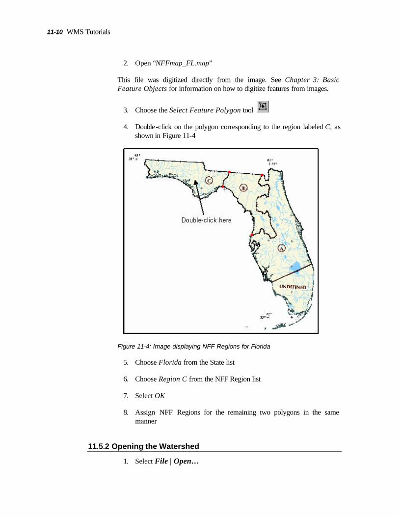
11-10 WMS Tutorials
2. Open “NFFmap_FL.map”
This file was digitized directly from the image. See Chapter 3: Basic Feature Objects for information on how to digitize features from images.
3. Choose the Select Feature Polygon tool
4. Double-click on the polygon corresponding to the region labeled C, as shown in Figure 11-4
Figure 11-4: Image displaying NFF Regions for Florida
5. Choose Florida from the State list
6. Choose Region C from the NFF Region list
7. Select OK
8. Assign NFF Regions for the remaining two polygons in the same manner
11.5.2 Opening the Watershed
1. Select File | Open…

NFF Program Interface 11-11
2. Open “NFF_FL.wpr”
At this point, the study area appears as a small polygon. You will zoom in to better distinguish the area.
3. Choose the Zoom tool
4. Zoom in on the region indicated in Figure 11-5
Figure 11-5: Zoom in on the watershed.
5. Select Display | Display Options…
6. Choose the DEM tab
7. Toggle off the check box for displaying DEM Contours
8. Select OK
9. Select Feature Objects | Compute Basin Data…
10. Select the Current Coordinates button
11. Make sure the Horizontal and Vertical units are set to Meters
12. Select OK twice

11-12 WMS Tutorials
11.5.3 Running NFF
1. Switch to the Hydrologic Modeling module
2. Make sure Model combo box is set to NFF
3. Choose the Select Basin tool
4. Double-click on the icon for Basin 1B
5. Select Yes
Notice that the regression equation is automatically selected. Also, if our basin had overlapped with another NFF region, the areas and percentages of overlap for each region would also have been calculated.
6. Enter 10.8 for the Lake Area variable
7. Select the Compute Results button
8. Select Done
As you can see, the NFF Region coverage allows WMS to automatically load the appropriate regression equation(s) when we open the NFF dialog. Now, this might not save us a great deal of time if we are only running the simulation once for a single basin. However, if we plan to study many different basins on a regular basis, then creating an NFF Region coverage for our state would prove to be very efficient.
11.6 Conclusions
In this tutorial, we have discussed the following concepts in conjunction with setting up an NFF simulation:
1. How to calculate important parameters with the Compute Basin Data command
2. How to use the Compute Coverage Overlay calculator to compute areas of overlap between our drainage basin and any other coverage type
3. How to use an NFF Region coverage to automatically determine which equations should be used and to compute any areas of NFF region overlap

NFF Program Interface 11-13

12 Time of Concentration Calculations and Computing a Composite CN
CHAPTER 12
Time of Concentration Calculations and Computing a Composite CN
Estimated Time: 30 minutes.
Travel times (time of concentration, lag time, and travel time along a routing reach) are critical to performing analysis with any of the hydrologic models. In this tutorial you will learn about the two different ways WMS can be used to compute time of concentration for a TR-55 simulation (lag times are computed in the same way):
• Runoff distances and slopes for each basin are automatically computed whenever you create watershed models from TINs or DEMS and compute basin data. These values can then be used in one of several available equations in WMS to compute lag time or time of concentration.
• If you want to have a little more control (and documentation) over the lag time or time of concentration, you will use a time computation coverage to define critical flow paths. Time computation coverages contain flow path arc(s) for each sub-basin. An equation to estimate travel time is assigned to each arc and the time of concentration (or lag time) is the sum of the travel times of all arcs within a basin. Lengths are taken from the length of the arc and slopes derived if a TIN or DEM are present.
In this tutorial you will compute the time of concentration for the two sub-basins and the travel time between outlet points in the watershed shown below. You

12-2 WMS Tutorials
will use the TR-55 library of equations, but you could just as easily use one of the other pre-defined equations, or enter your own equation.
A=0.10 mi^2 A=0.12 mi^2
Figure 12-1 American Fork Watershed
Many hydrologic models, including TR-55, use a composite curve number to account for losses. A composite curve number is computed for each basin by overlaying land use and soil type polygons.
12.1 Reading a TIN File
You will first read in a TIN that has already been processed and used to delineate two sub-basins. The TIN serves the same purpose as a drainage coverage combined with a DEM.
1. Switch to the Drainage Delineation module
2. Select File | Open…
3. Open “aftr55.tin”
4. Select TIN | Compute Basin Data…
5. Select the Current Coordinates button
6. Make sure that the Horizontal and Vertical units are set to U.S. Survey Feet
7. Select OK
8. Select Square miles for Basin Areas, and Feet for Distances

Time of Concentration Calculations and Computing a Composite CN 12-3
9. Select OK
10. Select Display | Display Options…
11. Choose the TIN tab
12. Toggle off the check box for Triangles
13. Choose the TIN Drainage tab
14. Toggle on the box for displaying Drainage Basin Boundaries
15. Select OK
Your display should now show the basin boundaries and stream network.
12.2 Defining Flow Path Arcs
Flow paths can automatically be traced across a TIN (or DEM with flow directions computed) using the flowpath tool. You can take advantage of this functionality in WMS to set up your flow path segments.
1. Select the Map module
2. Expand the Map Data folder in the Data Tree
3. Right-click on the General coverage in the Data Tree
4. Select Properties… from the pop-up menu
5. Set the Coverage type to Time Computation
6. Select OK
7. Select the Create Feature Points tool
8. Create feature points at the two locations marked by an X in the figure below. Be sure that there is one point inside of each basin boundary.

12-4 WMS Tutorials
A=0.10 mi^2 A=0.12 mi^2
x
x
Figure 12-2: Starting Locations for Time of Concentration Arcs.
These points represent the furthest point from the outlet for their respective basins. Now feature arcs will be created from these points to the outlet by following the flow path.
1. Select the Select Feature Point/Node tool
2. Select both feature points just created (use the <SHIFT> key to multi-select)
3. Select Feature Objects | Node->Flow Arcs
4. Choose the Create multiple arcs option
5. Select OK
The Create multiple arcs option will cause WMS to break the flow path arcs once they enter the stream defined on the TIN. The TR-55 method (others are similar as well) uses three different flow segments to compute time of concentration: sheet flow (up to 300 feet), shallow concentrated flow, and open channel flow. Since WMS will automatically break the arcs between overland and channel flow, two of three segments will already be defined. You will need to separate the sheet flow from the shallow concentrated flow before setting up the equations.
1. Select the Select Feature Vertex tool
2. The figure below identifies locations approximately 200-300 feet downstream from the beginning of the flow path arc. Select one of these vertices.
3. Select Feature Objects | Vertex<->Node

Time of Concentration Calculations and Computing a Composite CN 12-5
4. Repeat for the other flow arc (alternatively you could multi-select the two vertices and convert them to nodes at the same time).
Figure 12-3: Locations to Break Sheet Flow Segments.
You should now have three arc segments for each basin. These arcs will be used to compute a time of concentration for the TR-55 analysis. However, we will also want to compute a travel time for the flow from the upper basin to the lower basin. This will require a flow path segment between the upstream outlet and the lower outlet. The flow path arcs from the lower basin already include flow for part of this distance, but there remains a segment for which no flow path arc exists.
1. Select Feature Objects | Streams->Flow Arcs
This will create an arc that joins the outlet of the upper basin with the flow path segment already created for the lower basin. Where the flow path segments meet the arc from the lower basin is split into two. This will leave four arcs to define time of concentration for the lower basin (two will actually be in the stream). The arc just created, while in the lower basin, will not be used when computing time of concentration.
You have used the Node->Flow Arcs and Streams->Flow Arcs commands to automatically generate the flow path segments from flow on a TIN. Similarly, arcs could have been created from flow on a DEM with flow directions, or they
could be created manually using the create arc tool . When defining arcs manually you must keep in mind that just like stream arcs in the drainage coverage, direction is important. Time computation arcs should be defined from downstream to upstream.

12-6 WMS Tutorials
12.3 Assigning Equations to Time Computation Arcs
With the flow path segments defined you are now ready to assign equations that will be used to determine a travel time for the arc. Use the following figure as a guide while defining the equations.
87
6
54
3
2
1
Figure 12-4: Time Computation Arcs.
1. Choose the Select Feature Arc tool
2. Double-click on the arc labeled 1
By default the arc will be a TR-55 sheet flow equation arc, so all you need to do is define the overland manning’s roughness coefficient and the 2yr-24hr rainfall. Length and slope will already be defaulted from the selected arc.
1. Click on the n Mannings line in the Variables text window
2. Enter a value of 0.24 in the Variable value edit window
3. Click on the rainfall line in the Variables text window
4. Enter a value of 1.1
You should notice in the Instructions/Results window that you are told what variables need to be defined before a travel time can be computed. Once you have entered all the necessary values, this same window reports the travel time for this arc. In this way, you can compute travel time for any arc segment no matter what the application is.
1. Select OK

Time of Concentration Calculations and Computing a Composite CN 12-7
2. Repeat the previous steps for the arc labeled 4. Use a Manning’s roughness of 0.15 and a rainfall value of 1.1
3. Select OK
You have now defined equations for the overland sheet flow segments in each basin and are ready to define the next two arc segments as shallow concentrated flow.
1. Double-click on the arc labeled 2
2. Change the equation type to TR-55 shallow conc eqn
3. Click on the Paved line in the Variables text window
4. Enter no in the Variable value edit window
5. Select OK
6. Repeat for the arc labeled 5, using the same arc type. In this case set the Paved value to yes
The remaining arcs will be defined as open channel flow arcs.
1. Double-click on the arc labeled 3
2. Change the arc type to TR-55 Open channel eqn
3. Click on the Manning’s n line
4. Enter a value 0.016 in the Variable value edit window
5. Select the hydraulic radius line in the Variables window
6. Select the Hydraulic Radius button to open up the channel calculator so that the hydraulic radius can be computed from rough estimates
7. Change the Channel type to Rectangular
8. Enter a Longitudinal slope of 0.0015
9. Enter a Channel width of 3.0
10. Choose the Enter depth option
11. Enter a depth of 0.33 (an approximated depth since we do not know what the flow is at this point)

12-8 WMS Tutorials
12. Select the Calculate button
13. Select OK for both dialogs
You have now defined the necessary parameters for computing travel time using the TR-55 open channel flow (Manning’s) equation. Repeat for the arcs labeled 6, 7, and 8 using the following values:
Arc Manning’s N Hydraulic Radius 6 0.016 0.35 7 0.016 0.41 8 0.016 0.38
If you wish you can continue to experiment with the channel calculator to compute the hydraulic radius rather than entering the given values.
You now have defined equations and variable values for each flow path segment. You can change these equations, variables, add new flow path segments, etc. in order to determine the best flow paths and most appropriate equations for each basin. In other words, this process is subjective and it may take a few iterations to get the best value.
12.4 Using the Time Computation Arcs to Compute Time of Concentration for a TR-55 Simulation
Before assigning time of concentrations to each basin you need to decide which model you want to use. For this tutorial you will be running TR-55, but but the same time computation tools you learn in this tutorial could be used for any of the supported WMS models (such as in the TR-20 basin data dialog, the HEC-1 Unit Hydrograph method dialog, and the Rational Method dialog).
1. Select the Hydrologic Modeling module
2. Change the Model drop-down list to TR-55
3. Select TR-55 | New Simulation
4. Select TR-55 | Run Simulation…
5. Select the Select Basin tool while the TR-55 dialog is still open
6. Select the upper basin
7. Enter a Rainfall value of 1.5
8. Change the Rainfall distribution to Type II

Time of Concentration Calculations and Computing a Composite CN 12-9
9. Select the Compute Tc – Map Data button. You will see the three time computation arcs that are in the basin
10. You can create a detailed report as a text file if you want by selecting the Export Data or Copy to Clipboard buttons
11. Select Done
12. The sum of the travel times for these arcs will be used as the time of concentration for this basin
Note that you could bring up the time computation attributes dialog and change the equation or any of the equation variables by selecting the Edit Arcs button. Now you will set up the TR-55 basin data for the lower basin.
As a comparison you will now compute the time of concentration using the pre-computed runoff distance and slope parameters and one of the equations defined in WMS. To see the values that WMS has computed you will need to modify the display options.
1. Select the Done button to close the TR-55 dialog
2. Select Display | Display Options…
3. Choose the Drainage Data tab
4. Toggle on Max flow distance and Max flow slope
5. Select OK.
Notice that the longest flow path distance within a basin is displayed for each basin as well as the slope along that flow path. These are the variables that will be used in a separate equation to determine the time of concentration.
1. Double-click the upper basin icon to run TR-55 once again
2. Select the Compute TC - Basin Data button
In the Basin Time Computation dialog you can pick from one of several lag time or time of concentration equations that are pre-programmed in WMS (see WMS Help, topic: Overview of Basin Data Equations) for a complete description of these equations). You can also create your own equation from the computed variables, or parameters that you define yourself. In this tutorial we will use the Kerby equation for time of concentration, but you may wish to experiment on your own with some of the other equations or by making your own.

12-10 WMS Tutorials
1. Select the Compute Time of Concentration option from the Computation type drop-down box
2. Choose the Kerby method for overland flow equation in the drop-down list of equations. Notice that all variables needed for this equation are defined and so the time of concentration is reported in the text window at the top of the dialog
3. Select OK to close the Basin Time Computation dialog
You should notice that the time of concentration is very nearly the same as before (.57 hours).
At this point you might be wondering why you would ever want to create a time computation coverage and go through the effort of defining travel time arcs and assign equations to each if the same value can be determined using the parameters already computed from a TIN or DEM?
1. Select the Compute TC - Basin Data button again
2. Select the Kirpich method for overland flow on bare earth equation
3. Select OK
You should now set the time of concentration back to the one originally computed by the flow arc method. To do this:
1. Select the Compute Tc – Map Data button
2. Select Done
The lesson here is the equations using Basin Data work great if you are confident the equation represents the same kind of land surface you are dealing with. If not, you are likely better off to define equations along separate flow path segments using the Map Data. Of course, in either case you can customize the equations to suit your own needs.
1. Select the lower basin from the graphics window
2. Enter a Rainfall value of 1.5
3. Change the Rainfall distribution to Type II
4. Select the Compute Tc – Map Data button
This time you will notice that there are more than three arcs. This is because one of the flow path arcs (the one labeled 8 above) will be used to compute travel time between outlets but still is within the lower basin. Notice that WMS

Time of Concentration Calculations and Computing a Composite CN 12-11
defaults its status to inactive. WMS will try to make the best choice of arcs that are used for time of concentration for a basin, but at times you may need to set the active/inactive status on your own.
1. Select Done
12.5 Using the Time Computation Arcs to Compute the Travel Time Between Outlet Points
Besides using time computation arcs for computing time of concentration or lag time for a basin, you can also use them to compute the routing travel time of a channel.
1. Choose the Select Outlet tool while the TR-55 dialog is still open
2. Select the upstream outlet (the outlet to the upper basin)
3. Select the Compute travel time… button in the TR-55 dialog
4. Make sure that both of the downstream arcs are active (The active status in the dialog is turned on for both)
5. Note the time of concentration for these arcs
6. Select Done
7. The time of concentration from the arcs should now appear in the Travel time box.
8. Select Done to close the TR-55 dialog
12.6 Computing a Composite Curve Number
In this part of the workshop, you will learn how to overlay land use and soil coverages on your delineated watershed in order to derive a curve number (CN).
1. Select the Map module
2. Select File | Open
3. Open “luse.jpg”

12-12 WMS Tutorials
This file is an image of land use regions for an area. You can either digitize the polygons as demonstrated in the basic feature objects tutorial or read in a prepared file that has this already done for you. To open the map file:
4. Open “luse.map”
12.6.1 Land Use Table
Now you need to create a land use table with ID's and CN's for each type of land use on your map. To create the table, complete the following steps:
1. Choose the Select Feature Polygon tool
2. Double-click on the area labeled 11
You can see from the WMS landuse ID section of the dialog box that the three land use ID's have already been added.
1. Make sure the Display SCS CN's check box is selected
2. In the Selected land use properties box, select the Land name line
3. In the Land Name edit box, type Residential
4. In the Selected land use properties box, select the SCS Soil Type A CN: line
5. In the Type A CN Value edit box, type 61
6. Repeat for Type B, C, and D, using values of 75, 83, and 87
7. In the WMS landuse ID box, select Land ID 13
8. Enter the appropriate land names and Type CN's from the table below
9. Repeat this procedure for the other landuse ID's
10. Choose Close to exit the dialog (you don’t want to choose apply or the last ID you are editing, 22, will be applied to the polygon you selected to open this dialog in the first place, 11)

Time of Concentration Calculations and Computing a Composite CN 12-13
Table 12-1: Landuses and CN's
ID Name Type A
CN Type B
CN Type C
CN Type D
CN 11 Residential 61 75 83 87 13 Industrial 81 88 91 93 22 Orchards, Groves, Vineyards, Nursuries 36 60 73 79
12.6.2 Computing Composite Curve Numbers
In order to compute composite curve numbers, WMS needs to know which type of soil underlies each area of land. You will need to create a soil type coverage, create soil type polygons, and enter soil type data in the same manner as for land use. For this tutorial, this has already been done for you. You will need to read in this file:
1. Select File | Open…
2. Open “soils.map”
3. Make sure the Select Feature Polygon tool is still the active tool
4. Select Feature Objects | Attributes…
5. Select Soil ID 0 from the WMS soil ID list
You will note that a soil with ID is automatically assigned to be Type A. Similar ID =1 is B, 2 is C, and 3 is D.
6. Select Close
7. Select Display | Display Options…
8. Toggle on Color Fill Polygons
9. Switch to the General tab
10. Toggle on Soil Type Legend
11. Select OK
Now it is easy to see which soil types are assigned to which polygons.
12. Select Display | Display Options…
13. Toggle off Color Fill Polygons
14. Select OK
12-14 WMS Tutorials
15. Switch to the Hydrologic Modeling module
16. Select Calculators | Compute GIS Attributes…
17. Make sure the SCS Curve Numbers option is selected in the Computation section of the dialog
18. Specify to Use a Soil type coverage for determining soil type
19. Select your soil type coverage name (“Soil Type”) from the Soil type coverage name: drop down list
20. Specify to Use a Land use coverage for determining land use
21. Select your land use coverage name (“Land Use”) from the Land use coverage name: drop down list
12.6.3 Importing Land Use and Soil Type Tables
You may have your land use and soil type tables stored in data files. Instead of manually assigning the data as you have here, you would read these tables in from this dialog using the Import button.
Whether you have manually created tables or read them in from files, you should see the land use ID's, CN's for each soil type, and land use descriptions in the window of the Mapping section.
1. Select OK to compute the composite CN's
The composite CN for each basin should now be displayed at the centroid of each basin.
12.7 More TR-55
While you were entering the data for each of the two basins you may have noticed that instructions are given in the TR-55 data window to let you know what must be entered before a peak Q can be determined. Once you enter all of the data the peak Q is computed and displayed in this same window. You can also get help for anything listed in this window.
1. Select the Select Basin tool with the TR-55 dialog still open
2. Select the upper basin
3. Select the line in the TR-55 data window where the peak Q is displayed

Time of Concentration Calculations and Computing a Composite CN 12-15
Notice that the TR-55 equation for computing peak flow is displayed in the help window. You can get help for missing data as well.
1. Change the Time of concentration to 0.0 and click somewhere else to update the dialog
2. Select the line in the TR-55 data window that instructs you to define a time of concentration
Now you are told the units for time of concentration as well as the available options for determining it in the TR-55 help window.
1. Reenter the time of concentration by typing in the appropriate value, or if you can’t remember use the Compute Tc – Map Data button again
2. Select the Compute Hydrograph(s) button
3. Select Done to close the TR-55 dialog
4. Choose the Select Hydrograph tool
5. Double-click on the hydrograph icon that is displayed by the upper basin to view the hydrograph in a separate window
12.8 Conclusions
This completes the tutorial on using the time computation coverage to compute time of concentration and travel times and the land use and soil coverages to compute a composite CN value. In the process you have also learned about the TR-55 interface.


13 HEC-RAS Analysis
CHAPTER 13
HEC-RAS Analysis
HEC-RAS was developed by the U.S. Army Corps of Engineers Hydrologic Engineering Center. HEC-RAS performs a step backwater curve analysis for either steady state or transient conditions to determine water surface elevations and velocities.
13.1 Objectives
In this tutorial, you will learn how to use the WMS River tools to construct a HEC-RAS steady flow model. This includes the following:
• Building the conceptual model
• Mapping the conceptual data to a hydraulic model representation
• Running the simulation within HEC-RAS
• Viewing results in WMS
13.2 Preparing the Conceptual Model
The first step to creating a HEC-RAS model is to create a conceptual model which defines the river reaches (layout and attributes), the position of cross-sections on those reaches (orientation and station values), bank locations, and

13-2 WMS Tutorials
material zones. The conceptual model will be used to create a network
schematic inside the River Hydraulic module .
We will create the conceptual model from a USGS quad map as well as scattered bathymetric (elevation) data in the form of a TIN.
1. Select File | Open…
2. Open “wmsras.img”
3. Select File | Open
4. Open “wmsras.tin”
The TIN clutters the screen, yet we want to know where it is so we don’t create our conceptual model outside the domain of our bathymetric data. To better see the image, we will turn off the display of TIN triangles, vertices, and contours, and turn on the TIN boundary. To do this:
5. Select the Display Options button
6. Select the TIN tab
7. Uncheck the Unlocked vertices toggle box (it may already be unchecked)
8. Uncheck the Triangles toggle box
9. Uncheck the TIN Contours toggle box
10. Make sure the Boundaries box is checked
11. Select OK
13.2.1 Creating the Coverages
We need to create a centerline coverage for our reaches and a cross-section coverage for our cross-sections. These will form the core of our conceptual model.
1. Switch to the Map module
2. Expand the Map Data folder in the Data Tree.

HEC-RAS Analysis 13-3
3. Right-click on the Map Data folder within the Data Tree and choose New Coverage
4. Set its coverage type to 1D-Hyd Centerline
5. Select OK
6. Create another new coverage and set its coverage type to 1D-Hyd Cross Section
7. Select OK
8. Activate the centerline coverage by single-clicking on its name in the Data Tree
13.2.2 Creating the Centerline and Bank Arcs
Centerline arcs are used to define the locations and lengths of the study reaches and assign their attributes. We will have a centerline following the main channel as well as the tributary on the west. As the flows below the reservoir in the tributary on the East of the Leith Creek are small, we will disregard that reach in our simulation. To create the centerline arcs:
1. Select the Create Feature Arc tool
2. Following the pattern in Figure 13-1, create the centerline of the main channel from upstream to downstream (HEC-RAS views a river in this direction and it will ultimately help define what is the left bank and right bank characteristics) by clicking points on the centerline one at a time. Double-click the last point to indicate that it is the end of the centerline.
Figure 13-1: Creating the Centerline arcs

13-4 WMS Tutorials
1. Create the arc for the west tributary, upstream to downstream, by clicking points on the centerline. Create the last point where the tributary meets the main channel by double-clicking on the main channel centerline. This splits the centerline of the main channel into two reaches.
This defines the centerline for the model in this simulation. It will consist of two reaches in the main channel (divided by the tributary), and one reach in the west tributary.
Bank arcs are used to define the locations of the banks and the over-bank distances. The next step is to create bank arcs along both sides of each centerline arc. To create the bank arcs:
1. Select the Create Feature Arc tool
2. Create new arcs where you estimate the bank locations to be, based upon contours/colors (roughly follow the green area around the centerline arcs) on the background image. Use Figure 13-2 as a guide.
Figure 13-2: Placement of Bank arcs
1. Choose the Select Feature Arc tool

HEC-RAS Analysis 13-5
2. Select all of the bank arcs (hold the <Shift> key down while selecting in order to multi-select arcs)
3. Select Feature Objects | Attributes…
4. Change the Arc Type to Bank
5. Select OK
The background image is no longer necessary. To turn it off:
1. Uncheck the toggle box next to the wmsras.img line in the Data Tree
13.2.3 Naming the Centerline Arcs
Reaches are stream sections where the flow rates and other hydraulic conditions are assumed to be constant. A river can be comprised of one or more reaches, but only one flow path. HEC-RAS has the ability to model multiple rivers (flow paths). To assign names to our rivers and reaches:
1. Double-click the uppermost reach in the main channel
2. Make sure the Arc type is set to Centerline
3. Select OK
4. Enter Leith Creek for the River Name
5. Enter Upper Main for the Reach Name
6. Select OK
7. Repeat steps 1 to 4 for each reach in the map as shown in Figure 13-3. (Note: For the Lower Main reach you can choose Leith Creek from the river name combo box instead of typing it in).

13-6 WMS Tutorials
Figure 13-3: River and Reach Names
13.2.4 Creating Land Use / Materials Coverage
One of the properties HEC-RAS uses is roughness values. We will designate materials to different areas of our model. Later we will assign each material a roughness value. The material zones are stored in WMS as coverage type Area Property . To load the materials data:
1. Select File | Open…
2. Open the file “Materials.map”
3. Select Edit | Materials…
4. Click the New button 5 times in order to create 5 new material types
5. Rename the materials as shown below in Figure 13-4

HEC-RAS Analysis 13-7
Figure 13-4: materials for use in the Area Property coverage
1. If you wish, you may set the color and pattern to better match the descriptions.
2. Select OK to close the Materials Data dialog
3. Make sure the newly created Area Property coverage “materials” is active in the Data Tree
4. Right click on the Materials layer and choose Properties…
5. Change the Coverage type from General to Area Property .
6. Select OK
Now that you’ve defined all the materials, you will assign a material type to each polygon in the “materials” coverage. To better distinguish the material polygons, we will hide the image
7. Select the Select Feature Polygon tool
8. Select the polygon that defines the river area (see Figure 13-5)
9. Select Feature Objects | Attributes…
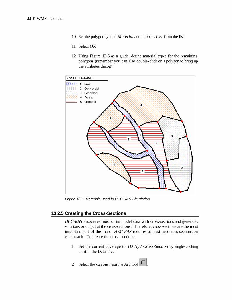
13-8 WMS Tutorials
10. Set the polygon type to Material and choose river from the list
11. Select OK
12. Using Figure 13-5 as a guide, define material types for the remaining polygons (remember you can also double-click on a polygon to bring up the attributes dialog)
Figure 13-5: Materials used in HEC-RAS Simulation
13.2.5 Creating the Cross-Sections
HEC-RAS associates most of its model data with cross-sections and generates solutions or output at the cross-sections. Therefore, cross-sections are the most important part of the map. HEC-RAS requires at least two cross-sections on each reach. To create the cross-sections:
1. Set the current coverage to 1D Hyd Cross-Section by single-clicking on it in the Data Tree
2. Select the Create Feature Arc tool .

HEC-RAS Analysis 13-9
3. Create at least two cross-sections on each reach by clicking a point on one side of the reach then double -clicking a point on the other side of the reach as shown in Figure 13-6
Figure 13-6: Cross-section coverage
13.2.6 Extracting Cross-Sections
In the cross-section coverage, all arcs are cross-section arcs. Their position and orientation define the location of the cross-sections in the system, but as of yet, they do not have any data assigned. We want to assign elevation data, materials, and point property locations to the cross-sections. This information will be extracted from the TIN, the area property coverage, and the centerline coverage. To extract this data:
1. Select River Tools | Extract Cross Section…
2. WMS will extract an elevation point at every triangle edge along the cross-section arc. The default extraction settings are to use the Centerline coverage to generate point properties and the Area Property coverage to define material zones.
3. Select OK

13-10 WMS Tutorials
4. When WMS prompts you for filename and location for saving the cross-section database, enter the name xsecs and select Save
Each cross-section arc now stores a link to a cross-section database record which contains xyz data, materials properties, bank locations, and thalweg locations. To view and edit the information at a cross-section:
5. Choose on the Select Feature Arc tool
6. Double click on any cross-section. This brings up the River Cross Section Attributes dialog
7. Make sure that the reach name is assigned correctly
8. Click on the Assign Xsec button. This brings up the Assign Cross Section Profile dialog, which is used to view the current cross section shape and select a different cross-section from a cross-section database if desired
9. Click on the Edit button. This brings up the Cross-Section Attributes dialog. This dialog can be used to view and/or edit the cross-section
10. Click on the Line Props tab to view the materials that are assigned to the cross-section
11. Click on the Point Props tab to view the locations of the left bank, right bank, and thalweg
12. Select Cancel until all the dialogs are closed
For this tutorial we will use the cross sections as extracted from the TIN, but often for a project you will need to edit a cross section, or merge surveyed cross sections and other editing procedures. This is the topic of a separate tutorial and therefore is not covered in detail here.
13.3 Creating the Network Schematic
WMS interacts with HEC-RAS using a HEC-GeoRAS geometry file. This file contains the cross-sectional data used by HEC-RAS in addition to three dimensional georeferencing data. To create this geometry file the conceptual model must be converted to a network schematic diagram in the River Module. To convert the conceptual model to a network schematic:
1. Make sure you are still in the Map module
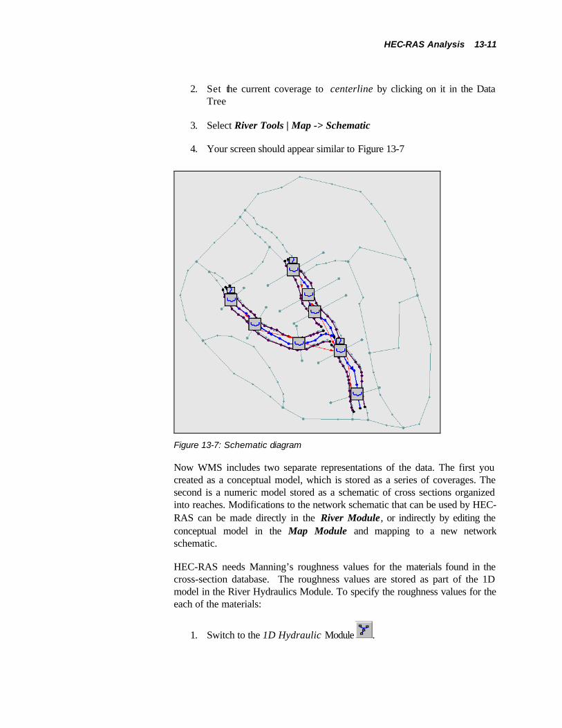
HEC-RAS Analysis 13-11
2. Set the current coverage to centerline by clicking on it in the Data Tree
3. Select River Tools | Map -> Schematic
4. Your screen should appear similar to Figure 13-7
Figure 13-7: Schematic diagram
Now WMS includes two separate representations of the data. The first you created as a conceptual model, which is stored as a series of coverages. The second is a numeric model stored as a schematic of cross sections organized into reaches. Modifications to the network schematic that can be used by HEC-RAS can be made directly in the River Module, or indirectly by editing the conceptual model in the Map Module and mapping to a new network schematic.
HEC-RAS needs Manning’s roughness values for the materials found in the cross-section database. The roughness values are stored as part of the 1D model in the River Hydraulics Module. To specify the roughness values for the each of the materials:
1. Switch to the 1D Hydraulic Module .

13-12 WMS Tutorials
2. Select HEC-RAS | Material Properties
3. Enter the roughness values for each material as shown in Figure 13-8
Figure 13-8: HEC-RAS Material Properties Dialog
1. Select OK
Now we need to tell HEC-RAS which set of line properties in the database should be used as material types. To do this:
2. Select HEC-RAS | Model Control
3. Select the line property name that stores the roughness values for the cross-section database. In this case, the line property is named Materials which came from our Area Property coverage Materials
4. Select OK
13.4 Creating the Geometry Import File
Now that the model has been setup, we need to create the geometry file. To create this file:
1. Select HEC-RAS | Export GIS File...
2. Name the file hecras.geo

HEC-RAS Analysis 13-13
3. Select Save
After saving out the GIS file, WMS automatically opens the HEC-RAS application, loads the GIS file, and creates a new HEC-RAS project named “hecras.prj .”
13.5 Using HEC-RAS
Within HEC-RAS, we will setup and run the simulation and then export the results for post-processing in WMS. The setup will include entering junction lengths, specifying flow values, and assigning river boundary conditions.
1. Select Edit | Geometric Data…
2. Select OK to the message that the view extents need to be increased
3. Select View | Set Schematic Plot Extents…
4. Select the Set to Computed Extents button
5. Select OK
Your screen should appear like Figure 13-9below:
Figure 13-9: The Geometric Editor in HEC-RAS.

13-14 WMS Tutorials
In the case that an excessive number of points are extracted from the cross-section arcs, HEC-RAS has a tool that will filter points that are too close together to run an analysis. Since there are many data editing tools available within HEC-RAS in addition to the filtering tool, we simply make you aware of such tools and suggest that you browse the HEC-RAS user’s manual for more information.
First, we will enter junction lengths in the Geometric Data Editor.
1. Left-click on the node (junction) that joins the West Tributary and Upper Main reaches.
2. Select Edit Junction… from the pop-up menu
The Junction Length value should be entered as the distance stretching across the junction between adjacent cross-sections. We will measure these lengths with the Measure Tool in WMS.
3. Activate the WMS window
4. Switch to the Map module
5. Choose the Measure Tool
6. As shown in the example in [fig] below, trace out the distance along the centerline arc between the most downstream cross section arc on the West Tributary reach and the most upstream cross section arc on the Lower Main reach

HEC-RAS Analysis 13-15
Figure 13-10: Measuring Junction Lengths.
7. Revert back to the HEC-RAS Junction Data dialog
8. Enter the measured length in the Junction Length field corresponding to the “To: West Tributary – West Tributary” line
9. Repeat this step to measure and enter the Junction Length between the most downstream cross section arc on the Upper Main reach and the most upstream cross section arc on the Lower Main reach
10. Once you have finished entering both lengths, select OK
11. Select File | Exit Geometry Data Editor
The next step is to define the flow and boundary conditions for our reaches. To define this information:
1. Select Edit | Steady Flow Data
2. For Profile 1 (PF 1), enter 4000 for Upper Main; enter 5000 for Lower Main; enter 1000 for West Tributary
3. Click on the Reach Boundary Conditions button

13-16 WMS Tutorials
For our analysis we are going to have HEC-RAS compute normal depths at the boundaries of our model. To do this:
1. For each of the blank boxes in the spreadsheet, select the box and click on the Normal Depth button. Enter the following values for the slopes of each reach: 0.003 for the upper reach, 0.001 for the lower reach, and 0.005 for the tributary.
2. Select OK
3. Click the Apply Data button
4. Select File | Exit Flow Data Editor
We are now ready to run the steady flow analysis. We first need to set an option to set flow distribution locations so that velocity profiles will be computed. To set this option and perform the analysis:
1. Select Run | Steady Flow Analysis from the menu
2. Select Options | Flow Distribution Locations
3. Change the Global subsections to 3 in each of the three fields (LOB, Channel, and ROB)
4. Select OK
5. Click the Compute button. This runs the 1D analysis
6. Close the Steady Flow Analysis Dialog
7. Exit out of the HEC-RAS program
13.6 Post-Processing
Now that HEC-RAS has computed water surface elevations, we can read the solution into WMS. The water surface elevations are read in as 2D Scatter Points and can be used to perform a floodplain delineation. To read the solution:
1. In WMS, make sure you are in the 1D Hydraulic module
2. Select HEC-RAS | Read Solution…
3. Open “hecras.prj”
4. In the Data Tree, expand the 2D Scatter Data folder

HEC-RAS Analysis 13-17
Notice that a new scatter point file has been read into WMS. These points contain the water surface elevations computed by HEC-RAS. Since we used 7 cross-sections in our model, we only have 7 scatter points with which to perform the floodplain delineation. In order to achieve a more accurate floodplain delineation, however, WMS has a tool that interpolates scatter points along centerline and cross-section arcs.
1. Switch to the Map module
2. Select the 1D-Hyd Centerline coverage from the Data Tree
3. Select River Tools | Interpolate Water Surface Elevations…
4. Note that hecras is selected as the Scatter dataset. In this case, it is the only scatter dataset available. But if you had multiple datasets, you could specify which one to use for the interpolation.
5. Choose At a specified spacing for the Create a data point option
6. Enter 60 for the spacing
7. Select OK
8. Select the 1D-Hyd Cross Section coverage from the Data Tree
9. Select River Tools | Interpolate Water Surface Elevations…
10. Select OK
11. Switch to the Terrain Data module
12. Select Flood | Delineate…
13. Toggle on the Search radius check box and enter 1000 for the radius
14. Toggle on the Quadrants check box
15. Enter 4 for the number of stages in a quadrant
16. Select OK
17. WMS now computes two new datasets corresponding to floodplain depths and water surface elevations (river bed elevation + flood depth)
18. Expand the folder named New tin in the Data Tree
19. Expand the folder named W.S. (FLOOD) in the Data Tree

13-18 WMS Tutorials
20. Select the data set named W.S. Elev-PF 1 (FLOOD)
21. Select Display | Display Options…
22. Choose the TIN tab
23. Toggle on TIN Contours and choose the Contours button
24. Choose the Color fill between contours option
25. Select OK twice to exit both dialogs
These color-filled contours represent the varying water surface elevations in the computed floodplain. For more information and practice on flood plain delineation, see the chapter entitled Floodplain Delineation. A second HEC-RAS tutorial where surveyed cross sections are used can be found in chapter 19
Figure 13-11: Resulting TIN from the Floodplain Delineation

14 Floodplain Delineation
CHAPTER 14
Floodplain Delineation
This tutorial demonstrates how to perform a floodplain delineation with WMS. Before WMS can delineate a floodplain, users must provide it with an elevation TIN (Triangulated Irregular Network) and a scatter point data set with river stage values. TIN elevations might be obtained from survey data, or by converting DEM (Digital Elevation Model) points to TIN vertices. River stage files can be assembled manually, or read in from a HEC-RAS project file.
14.1 Objectives
This tutorial will familiarize you with how to delineate a floodplain based on 1) water surface elevations for a river and 2) a TIN, which represents the topography for the area. The tutorial will teach you how to:
• Experiment with the various Floodplain Delineation options, including input data, search radius, flow path, and quadrants
• Perform floodplain delineations with water surface elevations acquired by the following techniques:
1. Manually entered in a scatter point file
2. Approximated with the Channel Calculator in WMS
3. Computed with HEC-RAS
• Use a Flood Barrier coverage to restrict flood waters

14-2 WMS Tutorials
• Generate flood depth, impact, and extent coverages
14.2 Floodplain Delineation Options
You can choose from several different delineation options, which in turn affect how the floodplain is computed. Options include Search Radius, Flow Path, and Quadrants.
The Search radius determines how many TIN vertices are taken into account when performing the delineation. The Max search radius is the maximum distance that WMS will “look” from each scatter point to determine the intersection between the water surface and the land elevations. One method for choosing a value for the maximum search radius is to increase the radius until the floodplain extents no longer change.
The Flow path option ensures that the interpolated values for the floodplain are hydraulically connected.
The Quadrants option makes sure that water level data for interpolation is selected from all directions surrounding the point of interpolation rather than in just one direction (quadrant). In general, it is best to turn on the Quadrants option when computing a floodplain.
Users may want to run several floodplain delineations with varied options in order to see how the floodplain changes. Optimal settings for the delineation options vary with model geometry. For more details on these delineation options, refer to the WMS help file.
To experiment with some of the delineation options, we will open a TIN and a scatter point set. The TIN contains the land surface elevations and the scatter set contains water surface elevations.
1. Select File | Open…
2. Open “flood.tin”
In order to simplify the screen, we will turn off the display of TIN vertices and triangles.
3. Select Display | Display Options…
4. Choose the TIN tab
5. Toggle off the check box for Unlocked Vertices (it may already be off)

Floodplain Delineation 14-3
6. Toggle off the check box for Triangles
7. Select OK
8. Select File | Open…
9. Open “samplescatter.wpr”
10. Expand the Terrain Data folder in the Data Tree.
11. Expand the Land TIN in the Data Tree, this way you will be able to see the water surface elevation solution data sets.
12. Select Flood | Delineate…
13. Enter 100 for the Max search radius
14. Enter sr100 for the solution name
15. Select OK
16. We will now change the Search radius and re-calculate a floodplain
17. Select Flood | Delineate…
18. Increase the Max search radius to 500
19. Change the solution name to sr500
20. Select OK to delineate a new floodplain
21. Examine the flood depth solution by expanding the sr100 (FLOOD) solution folder and selecting the sr100_fd data set.
22. Viewing the other flood depth solution reveals a significant difference between the two floodplain delineations. The floodplain extends quite a bit further for the 500 search radius than for the 100 search radius.
23. Delineate two additional floodplains using Max search radii of 1000 and 2000
24. Expand their solutions in the Data Tree window and select the correspond flood depth data sets (sr1000_fd and sr2000_fd)
You’ll notice that there is very little difference between the floodplains delineated with search radius values of 1000 and 2000. Therefore, we can use a value of 1000 since we have found that increasing the radius doesn’t change the delineation appreciably.

14-4 WMS Tutorials
Now, we will experiment with using different Flow path values.
25. Select Flood | Delineate…
26. Enter 1000 for the Max search radius
27. Toggle on the Flow path check box
28. Enter 500 for the Max flow distance
29. Rename the solution as fp500
30. Select OK
31. Delineate two additional floodplains by using Max flow path values of 1500 and 3000 and examine their solution sets.
Once again, since there is little variation in these latter two delineation. Therefore, we might leave our Flow path value at 1500. As a note, when the TIN includes an area of unusually high elevations near the river (such as a levee), it is a good idea to use the Flow paths option.
Experiment further with the display options until you get a feel for how they change the floodplain delineation.
14.3 Creating a Scatter Point File
A scatter file, similar to the one you opened in the previous section, can be created with any text editor or spreadsheet application. The required input for the file are (x, y) coordinates for each data point, and a corresponding data set (in this case, the data set would be water surface elevation values for each coordinate). Each coordinate may be associated with more than one data value. Figure 1-5 shows the file format for a 2D scatter point file:
ID X Y “dataset 1” “dataset 2” … 1 2343 32322 34.3 45.7 … 2 2348 32318 33.9 45.4 … 3 2350 32316 33.5 45.0 … etc
Figure 14-1: File format for 2D scatter point file
1. Select File | New
2. Select OK

Floodplain Delineation 14-5
For this tutorial, the scatter file has been created for you. We will open it with a text editor to view how it is set up:
3. Select File | Edit File…
4. Open “wse.txt”
5. Select OK to open the file with Notepad
The datasets for the water surface elevations are named “WSE1” and “WSE2.” The WSE1 data set might represent current water levels, and WSE2 might represent expected levels given future developments, such as a proposed levee.
6. Close Notepad
14.3.1 Open the Scatter Point Data
1. Select Flood | Read Stage File…
2. Open “wse.txt”
3. Select File | Open…
4. Open “flood.tin”
14.3.2 Delineate the Floodplain
1. Select Flood | Delineate…
2. Choose WSE1 from the Select stage data set list
3. Change the Max search radius to 1500
4. Toggle off the Flow path check box
5. Change the Number of stages in a quadrant to 3
6. Select OK
7. This will begin the delineation process for the first set of water surface elevations. When WMS finishes, delineate a new floodplain based on the second set of elevations:
8. Select Flood | Delineate…
9. Choose WSE2 from the Select stage data set list

14-6 WMS Tutorials
10. Select OK
14.3.3 Creating a Flood Impact Map
WMS can use two separate floodplain delineations to generate a Flood Impact coverage.
A Flood Impact coverage shows the difference between two flood depth or water level sets. The differences are divided into ranges or classes. Using the floodplains delineated in the previous steps, you will create a Flood Impact coverage in order to investigate the difference in flooding with and without the proposed levee.
1. Select Flood | Conversion | Flood -> Impact Map…
2. Choose WSE1_fd in the Original data set combo box
3. Choose WSE2_fd in the Modified data set combo box
4. Toggle on the Create no impact polygons check box
5. Select OK to accept the default classes, ranges, attributes, and names
6. Select Yes to create the coverage
7. This new data set is calculated as WSE1_fd – WSE2_fd indicating that all values in the second data set were subtracted from their corresponding values in the first data set.
8. Switch to the Map module
9. Choose the Select Feature Polygon tool
10. Double-click on any one of the polygons
11. The dialog that opens shows the amount of change from the original data set to the modified data set, as well as the impact class ID and name.
Besides creating a tabular data file as described above, scatter point sets can also be created interactively with the tools in WMS, or opened from a HEC-RAS solution file. The following sections demonstrate these two methods for constructing scatter point data to be used in a floodplain delineation.

Floodplain Delineation 14-7
14.4 Creating Scatter Points with the Channel Calculator
Users can interactively create scatter points in the 2D Scatter Point module and enter a water surface elevation for each point. This section will demonstrate this method. To begin, we will clear all data from WMS and begin afresh.
1. Select File | New
2. Select OK when asked if you are sure you want to clear everything
WMS has a tool that allows us to interactively create scatter points and assign a data value to each point. The values for water surface elevations might be obtained by digitizing from a background image, or from another source. You can also use a cross section coverage in conjunction with the channel calculator to create scatter points with calculated depths along a river centerline.
For this example, we will use the Channel Calculator to compute water depths for various cross-sections in our channels and create a scatter point at each cross-section arc. The water surface elevation will be equal to the water depth computed by the Channel Calculator plus the ground elevation (given by the TIN).
We will begin by opening a MAP file containing a Cross Section coverage. This coverage contains several cross-section arcs along our stream reaches.
14.4.1 Open the Cross-section Arcs and River Centerlines
1. Select File | Open…
2. Open the file named “flood.tin”
3. Select File | Open…
4. Open “cross_section.map”
5. Make sure you are in the Map module
6. Right click on the Map Data folder in the Data Tree and select New Coverage from the pop-up menu
7. Change the Coverage type to 1D-Hyd Centerline
8. Select OK
9. Select File | Open…
10. Open “reaches.shp”

14-8 WMS Tutorials
11. Select OK
12. Select the Cross-Section coverage from the Data Tree window so that it will be the active coverage.
14.4.2 Define Manning’s Roughness Values for Cross Sections
13. Choose the Select Feature Arc tool
14. Select Feature Objects | Attributes…
This dialog displays the cross-section elevations and allows you to edit the cross-section stations and/or elevations, and to assign Manning’s roughness values. We will increase the Z scale to better distinguish the elevations:
15. Change the Z scale to 25:1
16. Choose Cross section 1 from the list of Cross Sections
17. Select the Edit multiple n values button
18. Enter a value of 0.03
19. Select OK
20. Select OK when asked if you want to change all Manning’s n values
21. Repeat the above steps to assign Manning’s n values to the remaining cross-sections as shown in the following table
Cross Section Name
Manning’s n
Cross section 2 .023 Cross section 3 .033 Cross section 4 .026 Cross section 5 .031 Cross section 6 .027
1. Select OK to close the Attributes dialog when you have finished defining all Manning’s n values
14.4.3 Using the Channel Calculator to Compute Depths
The Channel Calculator is a good tool for approximating channel flows or flow depths. Given a flow rate, the Calculator can compute a flow depth, and vice versa. As we calculate flow depths, we need to jot down the depth values so we can recall them later when we create the 2D scatter points.

Floodplain Delineation 14-9
1. Switch to the Hydrologic Tree module
2. Select Calculators | Channels…
3. Change the Channel Type to Cross Section
4. Make sure that Cross section 1 is selected from the Cross section list
5. Change the Units to Metric
6. Enter a value of 0.002 for Longitudinal slope. This is an estimate for the ground slope in the vicinity of Cross section 1.
7. Enter a value of 450 for the flow
8. Select the Calculate button
9. Select the Create Stage Point button
10. Choose Cross section 2 from the Cross Section list
11. Repeat the previous steps to compute Depths and create a stage point for this and all remaining cross-sections. The following table provides Flow and Longitudinal slope values for use with each cross-section.
Cross Section Flow (cms) Slope Cross section 1 450 .0020 Cross section 2 450 . 0015 Cross section 3 300 . 0019 Cross section 4 300 . 0006 Cross section 5 150 . 0087 Cross section 6 150 . 0037
The Channel Calculator can also be used to generate a rating curve
1. Select the Compute Curves… button
The default is to create a rating curve for the entered flow vs. depth, but you can also create curves for all of the other options listed. Further, you can enter a depth in the Channel Calculator and compute Depth on the Y Axis vs. any of the listed options (Flow would replace the Depth option for the X Axis)
2. Select OK
You can right-click in the rating curve plot window to export the data to a spreadsheet if you want.
3. When you are done viewing the rating curve plot, close the plot window by selecting the X in the upper right corner of the window

14-10 WMS Tutorials
4. Select OK to close the Channel Calculator
14.4.4 Interpolating Stages along the Centerline
You should now have a scatter point created with a computed water surface elevation at each cross section where it intersects the centerline as shown in Figure 14-2. In order for the flood delineation to work better we want to interpolate values along the centerline.
Figure 14-2: Labels for each cross section.
1. Switch to the Map module
2. Make sure the 1D-Hyd Centerline coverage is active in the Data Tree (this should also activate the River Tools menu in the Model drop-down list).
3. Select River Tools | Interpolate Water Surface Elevations…
4. Set the Create a data point field to At a specified spacing
5. Enter 30 for the spacing

Floodplain Delineation 14-11
You should see many scatter points added along the centerline arcs, resulting in a view similar to that in Figure 14-3 (the symbol for scatter points may be different).
Figure 14-3: View of interpolated scatter points.
If your scatter points didn’t interpolate as shown above, the most probable reason is that the original scatter points were not placed close enough to the Centerline arc. In order to continue, delete the scatter point set and either try creating the points again, or open the sample scatter point set contained in “samplescatter.wpr”.
14.4.5 Delineate the Floodplain
1. Switch to the Terrain Data module
2. Select Flood | Delineate…

14-12 WMS Tutorials
3. Change the Max search radius to 1000
4. Toggle on the Flow path option and enter a Max flow path value of 1000
5. Select OK
6. Turn on the display of the Flood plain contours to view the results
We have finished delineating a floodplain based on the water elevations that we calculated on our own. The next section will describe how to open a set of scatter points that were entered into a text file.
14.5 Delineation from HEC-RAS Data
14.5.1 Reading the HEC-RAS solution
In this section, we will use water surface elevations computed as a result of a separate tutorial that builds a HEC-RAS project. First, we will read a WMS project file that contains a TIN and then import a HEC-RAS solution from a model developed from the TIN:
1. Select File | New
2. Select OK
3. Select the Terrain Data module
4. Select File | Open…
5. Open “flood.wpr”
6. To simplify the display, we will hide some elements of the model
7. Expand the Terrain Data folder from the Data Tree
8. From the Data Tree, hide the TIN by toggling off its check box
9. Select Display | Display Options…
10. Choose the River tab
11. Toggle off the River Hydraulic Schematic check box
12. Select OK
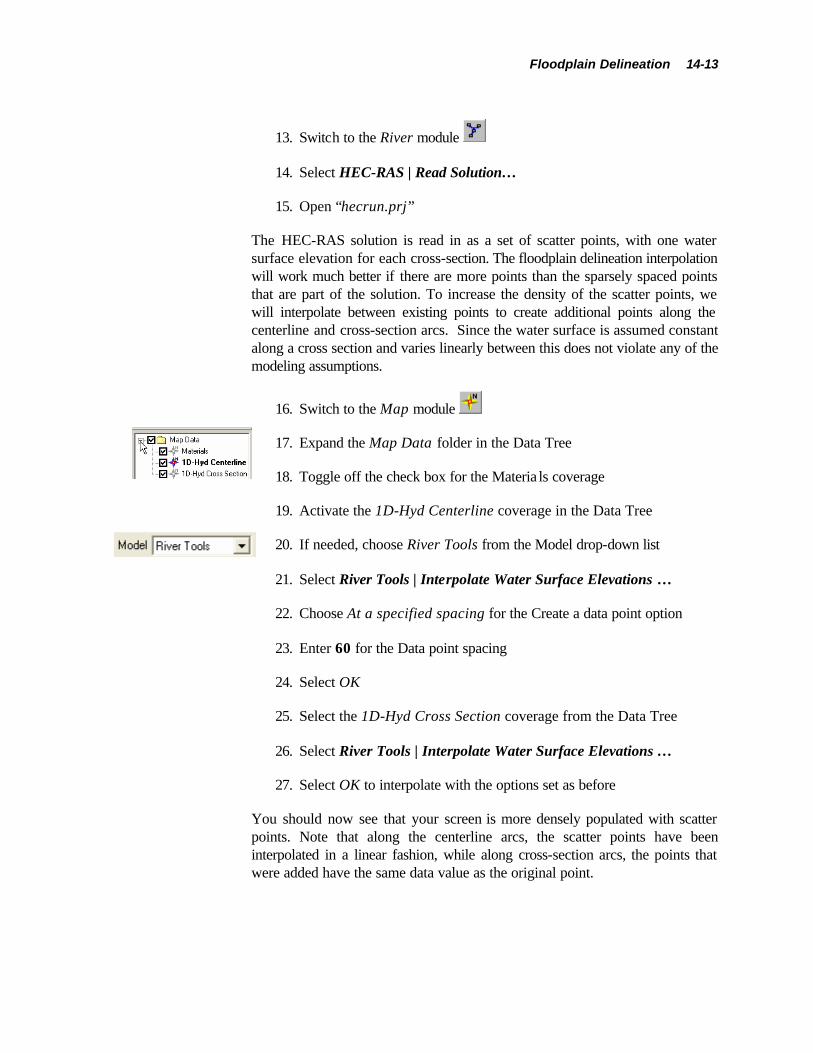
Floodplain Delineation 14-13
13. Switch to the River module
14. Select HEC-RAS | Read Solution…
15. Open “hecrun.prj”
The HEC-RAS solution is read in as a set of scatter points, with one water surface elevation for each cross-section. The floodplain delineation interpolation will work much better if there are more points than the sparsely spaced points that are part of the solution. To increase the density of the scatter points, we will interpolate between existing points to create additional points along the centerline and cross-section arcs. Since the water surface is assumed constant along a cross section and varies linearly between this does not violate any of the modeling assumptions.
16. Switch to the Map module
17. Expand the Map Data folder in the Data Tree
18. Toggle off the check box for the Materia ls coverage
19. Activate the 1D-Hyd Centerline coverage in the Data Tree
20. If needed, choose River Tools from the Model drop-down list
21. Select River Tools | Interpolate Water Surface Elevations …
22. Choose At a specified spacing for the Create a data point option
23. Enter 60 for the Data point spacing
24. Select OK
25. Select the 1D-Hyd Cross Section coverage from the Data Tree
26. Select River Tools | Interpolate Water Surface Elevations …
27. Select OK to interpolate with the options set as before
You should now see that your screen is more densely populated with scatter points. Note that along the centerline arcs, the scatter points have been interpolated in a linear fashion, while along cross-section arcs, the points that were added have the same data value as the original point.

14-14 WMS Tutorials
14.5.2 Using a Flood Barrier Coverage
WMS allows users to “confine” a delineation from the given elevation data by creating a flood barrier coverage. Arcs representing ridges or levees (existing or proposed) may be created in the model, and these in turn alter the floodplain delineation by restricting interpolation of the floodplain so that values on the “dry” side of the levee are not interpolated. In this tutorial, a map file of arcs representing a proposed levee will be used to demonstrate the effects of incorporating a flood barrier coverage.
1. Select File | Open…
2. Open the file named “levee.map”
Two new coverages are now added to the Map Data folder in the Data Tree. The coverage entitled proposed levee is a Flood Barrier coverage and breakline is a General coverage.
3. Verify that proposed levee is the active coverage in the Data Tree
4. Select the Zoom tool
5. Zoom in around the proposed levee as shown in Figure 14-4. The proposed levee is located along the west bank of the tributary stream.
Figure 14-4: Zoom in on the arc representing the levee
Contouring of floodplain data sets in WMS is based on TIN vertices. Therefore, it is important to make any necessary changes to the TIN before performing

Floodplain Delineation 14-15
floodplain delineation, especially if comparisons are to be made between different scenarios.
The flood extent is contoured to midpoints on triangle edges between flooded and dry areas.It is therefore recommended that a breakline be created on the “river side” of the flood barrier coverage in order to improve the visualization of the delineated floodplain. This breakline and the flood barrier are then forced into the TIN, effectively confining the flood contours between the two.
You will now force the flood barrier and breakline arcs into the TIN. The breakline is located immediately to the east of the flood barrier (you probably can’t see it unless you zoom in closely around the flood barrier arc).
To better distinguish the proposed levee and breakline arcs, hide the 1D-Hyd Centerline coverage.
1. Toggle off the check box for 1D-Hyd Centerline in the Data Tree
2. Choose the Select Feature Arc tool
3. Select the flood barrier arc
4. Select Feature Objects | Arcs -> Breaklines
5. When prompted, choose Use all arcs as breaklines
6. Select OK
7. At the next prompt, choose Interpolate Z values from existing TIN
8. Select OK
9. Activate the breakline coverage by selecting it from the Data Tree
10. Click on the Select Feature Arc tool
11. Select the breakline arc
12. Select Feature Objects | Arcs -> Breaklines
13. When prompted, choose Use all arcs as breaklines
14. Select OK
15. At the next prompt, choose Interpolate Z values from existing TIN
16. Select OK

14-16 WMS Tutorials
14.5.3 Delineating the Floodplain
Now that we have added the breaklines to our TIN, we are ready to delineate the flood plain:
1. Switch to the Terrain Data module
2. Select Flood | Delineate…
3. Choose the User defined flood barrier coverage option
4. Make sure the Search radius option box is toggled on and enter 1000 for the Max search radius
5. Enter 500 for the Max flow distance
6. Make sure the Quadrants check box is toggled on
7. Enter 4 for the Number of stages in a quadrant
8. We will accept the default solution and data set names
9. Select OK
It may take a minute or two for WMS to compute the floodplain delineation
10. From the Data Tree, toggle -on the TIN’s check box to show it again
11. Select the Frame Image macro
12. Expand the folder named Land
13. Expand the folder named W.S. Elev-PF 1 (FLOOD) in the Data Tree
14. Select the data set named W.S. Elev-PF 1_fd
15. Your screen should appear similar to Figure 14-5

Floodplain Delineation 14-17
Figure 14-5: Plot of floodplain depths
These contours correspond to the water depths in the floodplain area. To view the water surface elevation data set:
16. Select the data set named W.S. Elev-PF 1_wl from the Data Tree
14.6 Creating a Flood Extent Coverage
Flood depth and water level information are stored with the TIN, but WMS allows for the creation of feature objects from this data. In floodplain delineation, it may be useful to create a flood extent coverage. This coverage defines the boundary of the flood and may be exported for use in GIS applications. To create the flood extent coverage:
1. Select Flood | Conversion | Flood -> Extent Coverage…
2. Select W.S. Elev-PF 1_fd from the Select Flood Depth Data Set list

14-18 WMS Tutorials
3. Select OK (we will accept the default inundation limit and coverage name)
The flood extent boundary is converted to feature lines and WMS will try to build a polygon enclosing the flooded area. However in this case it reaches the boundary of the TIN and so a complete polygon is not available. You could close the polygon manually be creating an arc to along the TIN boundary and then choosing to Build Polygons.
14.7 Creating a Flood Depth Coverage
The flood extent coverage essentially divides the watershed area into two parts: flooded and not flooded. However, it is often necessary to know not only if an area is flooded but also how badly it is flooded.
It is common to divide the flooded area into zones, each with a depth range. In WMS, these zones are created by making a flood depth coverage. To create a flood depth coverage:
1. Select Flood | Conversion | Flood -> Depth Map
2. Select W.S. Elev-PF 1_fd from the Select Flood Depth Data Set combo box
3. Note the ranges and attributes of the five “zones” or “flood classes”
4. Select OK
5. Select the Zoom tool
6. Zoom in to view the bottom portion of the main channel
7. Switch to the Map module
8. Click on the Select Feature Polygon tool
9. Double-click inside a few of the polygons that have been created. This will bring up the flood extent attributes, which include the average flood depth for the zone.
14.8 Conclusions
After completing this tutorial, you should be familiar with using WMS to perform floodplain delineations in conjunction with:

Floodplain Delineation 14-19
• A flood barrier coverage
• Water surface elevations computed with HEC-RAS
• User-defined water surface elevations, created either interactively, or opened with a 2D scatter point file
• Post-processing in the form of creating Flood Extent, Flood Depth, and Flood Impact maps


15 Stochastic Modeling Using HEC-1 and HEC-RAS
CHAPTER 15
Stochastic Modeling Using HEC-1 and HEC-RAS
This tutorial demonstrates how to run a stochastic model within WMS. Since a certain degree of uncertainty usually exists in the selection of input parameters, running a stochastic model helps us explore multiple model solutions for differing input values. Users can specify a range of values to be used in the stochastic model.
15.1 Objectives
In this tutorial, you will learn the basics of setting up a stochastic model that will run the HEC-1, HEC-RAS, and Floodplain Delineation models simultaneously.
1. Assign key values to parameters
2. Define the Stochastic Model characteristics
3. Run the Model
4. View the solution means and probabilities
15.2 Opening the HEC-1 and HEC-RAS Models
Working HEC-1 and HEC-RAS models have been previously prepared for use in this tutorial. We will use the Stochastic modeling features of WMS to create

15-2 WMS Tutorials
a probabilistic map of floodplain boundaries. You may choose to review the development of these models in their separate tutorials.
There is generally a high degree of uncertainty associated with hydrologic modeling parameters such as the SCS Curve Number and rainfall depth. Using WMS you can vary these parameters stochastically in order to analyze a more complete parameter space and then use the results to reflect the known uncertainty in a flood plain delineation. The Stochastic Simulation will run a specified number of simulations using randomly generated values of basin Curve Numbers and basin precipitation for each simulation. Results from the HEC-1 run are then passed to a developed HEC-RAS simulation, and finally the results from HEC-RAS are used to compute a series of flood plain boundaries from which a probability of flooding, based on model parameter uncertainty can be computed.
1. Select File | Open…
2. Open “run1.wpr”
3. Run1.wpr is a WMS project file that calls in all of the prepared input data for the HEC-1 and HEC-RAS models. Each simulation has been previously tested to ensure that they can be run successfully.
15.2.1 Preparing the HEC-RAS model
1. To begin, we will zoom in on the HEC-RAS model domain.
2. Switch to the Tree module
3. Hide all basins and outlets by un-checking the box next to the Hydrologic Tree Data folder in the Data Tree
4. Switch to the Map module
5. Expand the Map Data folder in the Data Tree by clicking its + icon
6. Hide the coverage named Drainage by un-checking its visibility box in the Data Tree
7. Select the Frame macro
8. Activate the 1D-Hyd-Centerline coverage by single-clicking on its name in the Data Tree window

Stochastic Modeling Using HEC-1 and HEC-RAS 15-3
9. Select River Tools | Map -> 1D Schematic. This step initializes the HEC-RAS river scheme in preparation for reading in the HEC-RAS solution.
10. Switch to the River module
11. Select HEC-RAS | Read Solution…
12. Open “hecrun1.prj”
When we read in a HEC-RAS project file in which the water surface profiles have been calculated, a scatter point is placed at the thalweg location of each cross-section. Each scatter point contains the value of the water surface elevation at that point in the river reach. To create additional scatter points for interpolation purposes, we need to interpolate more scatter points along both the center-line and cross-section arcs.
13. Switch to the Map module
14. Make sure the 1D-Hyd-Centerline coverage is active in the Data Tree
15. Select River Tools | Interpolate Water Surface Elevations…
16. Set the Create a data point field to At a specified spacing
17. Enter 60 for the Data point spacing
18. Select OK
19. Activate the 1D-Hyd-Cross Section coverage from the Data Tree
20. Select River Tools | Interpolate Water Surface Elevations…
21. Select OK
This same data point spacing (60) will be used to interpolate each HEC-RAS solution along the reach and the cross sections when running the stochastic simulations.
15.2.2 Preparing the HEC-1 model
1. Show the Drainage coverage by checking its box in the Data Tree
2. Switch to the Tree module

15-4 WMS Tutorials
3. Show the contents of the Hydrologic Tree Data folder by toggling on its check box
4. Select the Frame macro
We will now assign key values to the parameters that we wish to randomly vary during the Stochastic run. Key values are negative integers that we assign to a parameter in lieu of the actual value. By entering a negative value for precipitation, for example, WMS replaces the precipitation value with a feasible precipitation value at run time. This precipitation value changes for each new run. Each generated value is based on a normal distribution, and can be controlled by specifying minimum and maximum allowable values.
5. Choose the Select Basin tool
6. Multi-select the basins labeled 2B and 3B by holding the <Shift> key as you single-click on each basin icon
7. Select HEC-1 | Edit Parameters…
8. Select the Precipitation button
9. Enter a value of -1 in the Average precipitation field
10. Select OK
11. Select the Loss Method button
12. Enter a value of -2 in the CRVNBR field
13. Select OK
14. Select Done
15. Multi-select the basins labeled 4B and 1B
16. Use the method shown in the previous steps to assign an Average precipitation value of -1 and a CRVNBR value of -3 to these basins
15.3 Running the Stochastic Model
For this tutorial, we have assigned key values only to HEC-1 parameters, namely precipitation and Curve Number. However, WMS also allows key values to be assigned to Manning’s N values for the HEC-RAS model, and Search Radius for the Floodplain Delineation model.

Stochastic Modeling Using HEC-1 and HEC-RAS 15-5
15.3.1 Setting Up the Model
1. Select HEC-1 | Stochastic Modeling…
Users can choose either a Monte Carlo or Latin Hypercube approach to generating values for the stochastic model. We will use the Monte Carlo approach for this exercise. When using the Monte Carlo method, we must specify the number of simulations that we want to run. With the Latin Hypercube approach, instead of specifying a number of simulations, we enter a number of segments for each variable. The total number of simulations for a Latin hypercube run is equal to the product of the number of segments for each variable. If we have 3 variables, with 3 segments each, then a Latin Hypercube model will run 27 times. Users also specify maximum, minimum, and starting values for each stochastic variable.
2. Select the Monte Carlo option for the Simulation type
3. Enter 5 for the Number of simulations
4. We specify 5 simulations for this tutorial in the interest of time. Remember, though, that statistical studies indicate that in order for the generated values to resemble a normal distribution, one should run at least 30 simulations.
5. Choose HEC-1 from the Selected model list box
6. Toggle on the Define stochastic model check box
7. Under the Filename parameters section, select the Base filename: button
8. Browse to the folder in which the HEC-RAS project file (“hecrun1.prj”) is located and enter hecrun1 as the File name
9. Select Save
10. Select the Add variable button 3 times to add 3 variables to the table
11. Refer to Figure 15-1 and enter the values shown for each stochastic variable
Figure 15-1: Values for the Stochastic Variables table

15-6 WMS Tutorials
12. Now, we will turn on stochastic modeling for the HEC-RAS and Floodplain models:
13. Change the Selected model list box to HEC-RAS
14. Toggle on the Define stochastic model check box
15. Select the Base filename button and browse to the same path as “hecrun1.prj”
16. Enter hecrun1 as the File name and select Save
17. Change the Selected model list box to Floodplain
18. Toggle on the Define stochastic model check box
19. Select the Base filename button and browse to the same path as “hecrun1.prj”
20. Enter hecrun1 as the File name and select Save
21. Select OK to exit the Stochastic Run Parameters dialog
22. Select File | Save to save your changes
15.3.2 Running the Model
The last step in setting up the stochastic simulation is linking the output hydrographs (in this case it is a steady state simulation and so only the peak flow is used) from the HEC-1 model to the HEC-RAS input boundary condition for the appropriate rivers and reaches.
1. Select HEC-1 | Run Stochastic Model…
2. Choose 2B Basin Hydrograph from the Select a hydrograph combo box
3. Choose Leith River from the Select a river combo box
4. Choose Upper Branch from the Select a reach combo box
5. Choose 2648.528 from the Select a cross-section list box
6. Select the Assign Hydrograph BC button
7. Repeat the previous steps to link the hydrographs and cross-sections shown in Table 15-1:

Stochastic Modeling Using HEC-1 and HEC-RAS 15-7
Table 15-1: Assigning additional hydrographs to cross-sections
Hydrograph River Reach Cross-section
3B Left Fork Branch 1703.086 5C Leith River Lower
Branch 759.138
2C Leith River Lower Branch
72.889
Before we use the Stochastic Model to run Floodplain Delineation over and over again, we need to change some of the delineation options. To set these options:
8. Select the Floodplain Delineation Options button.
9. Change the Max search radius to 1500
10. Make sure the Quadrants check box is toggled on
11. Enter 3 for the Number of stages in a quadrant
12. Select OK
13. Select OK to run the Stochastic simulations
Progress for the simulations will be displayed in the Stochastic dialog. You will be able to see the values selected for the CN and precipitation for each run as well as the diagnostic information for the models. It is possible to abort prematurely by selecting the Abort button.
15.4 Viewing the Results
All solutions (HEC-1 hydrographs, HEC-RAS river stages, and Floodplain delineations) are read into WMS. Furthermore, at the completion of the stochastic run, WMS computes a dataset containing the probabilities that flooding will occur at various locations within the original TIN. This is computed by assigning to each vertex in the TIN whether it was flooded or not. At the completion of all runs contours showing 0-100 percent probability of flooding can be viewed. 100% probability would mean that flooding occurred for the entire model, 50% probability would be flooding for half of the simulations, etc. To view the results:

15-8 WMS Tutorials
1. Select Close to exit the Stochastic HEC-1 wrapper
2. Switch to the Terrain Data module
3. Select Display | Display Options…
4. Choose the TIN tab
5. Toggle on the TIN Contours check box
6. Select OK
7. From the Data Tree, expand New Tin in order to see its subfolders
8. Expand the folder named hecrun1_prob(FLOOD)
9. Select the dataset named hecrun1_prob
10. By contouring this dataset, we see the probabilities that the floodplain will arrive at different locations.
11. Now, select the dataset named hecrun1_depth
This dataset contains the average depths from all of the stochastic simulations.

16 Storm Drain: Rational Design
CHAPTER 16
Storm Drain: Rational Design
Storm Drain is a hydraulic analysis and design program for storm drain systems. Developed by the Federal Highway Administration, Storm Drain provides hydraulic engineers with a quick and accurate method of computing the capacity of an existing system, or designing a system to meet a given set of input flows. The Storm Drain interface in WMS uses the same HYDRA program that has been distributed by the FHWA as part of their HYDRAIN computer program package for the past several years.
16.1 Objectives
In this tutorial, we will set up a drainage simulation based on the Rational Method for a proposed subdivision. The objective of this tutorial is to teach you the basic steps for defining a Storm Drain input file, running the numeric model, and viewing the results. These steps include the following:
1. Define runoff coefficients
2. Define the drainage area
3. Compute flows for each basin using the Rational Method
4. Import a pipe network
5. Define the necessary parameters for the network
16-2 WMS Tutorials
6. Link nodes from the drainage network to their corresponding nodes in the pipe network
7. Assign elevations to the pipe network
8. Save the Storm Drain input file and run the simulation
9. View the solution
16.2 Defining Runoff Coefficients
16.2.1 Reading in the Subdivision Layout and Elevations
We will open a shapefile containing the geography of the proposed subdivision. Also, to help us in defining elevations and slopes for the drainage area, we will open a TIN (Triangulated Irregular Network) for the area:
1. Select File | Open…
2. Open “cougarestates.tin”
3. Switch to the Map module
4. Right-click on the Map Data folder in the Data Tree
5. Select New Coverage from the pop-up menu
6. Change the Coverage type to Runoff Coefficient
7. Select OK
8. Select File | Open…
9. Open “cougarestates.shp”
10. Select OK to import the polygon shapefile
16.2.2 Defining the Runoff Coefficients
We will turn off the display of the TIN in order to better distinguish the subdivision polygons.
1. Switch to the Terrain Data module

Storm Drain: Rational Design 16-3
2. Expand the Terrain Data folder in the Data Tree
3. Toggle the visibility check box for the “new” TIN off in the Data Tree
4. Switch to the Map module
5. Choose the Select Feature Polygon tool
6. Double-click on the lower left polygon
7. Enter a runoff coefficient of 0.6
8. Select OK
9. Assign Runoff Coefficients for the remaining polygons as shown in Figure 16-1
Figure 16-1: Assigning runoff coefficients.
16.3 Defining the Drainage Area
First, we will initialize the Storm Drain interface. Initializing Storm Drain tells WMS to make available additional features needed to build a Storm Drain model. Then we will read in pre-defined drainage boundaries and set up drainage inlets and a drainage outfall.

16-4 WMS Tutorials
16.3.1 Initializing Storm Drain
1. Change the Model drop-down box located at the top of the WMS interface to Storm Drain
2. Select Storm Drain | New Simulation
16.3.2 Creating the Drainage Coverage
1. Right-click on the Map Data folder in the Data Tree
2. Select New Coverage from the pop-up menu
3. Change Coverage type to Drainage
4. Select OK
5. Select File | Open…
6. Open “runoff.shp”
7. Click on the browse button located under the check box for opening a shapefile of arcs
8. Open “drainage.shp”
9. Select OK to import the shape file data. Figure 16-2 shows what your layout should look like.

Storm Drain: Rational Design 16-5
Figure 16-2: Drainage basins and streams for the subdivision.
Before defining nodes as storm drains/drainage outlets, we will hide the Runoff Coefficient coverage in order to simplify the screen display
1. Toggle the visibility check box for the Runoff Coefficient coverage off in the Data Tree
2. Choose the Select Feature Point/Node tool
3. Double-click on the node labeled Drainage Outlet in Figure 16-2
4. Change the Point type to Drainage Outlet and select OK
5. While holding the <SHIFT> key, select each of the nodes labeled as Storm Drains in Figure 16-3. These points correspond to manhole locations in the pipe network. Be sure to select the nodes that intersect with the basin boundary lines.

16-6 WMS Tutorials
Figure 16-3: Storm Drain node locations.
6. Select Feature Objects | Attributes…
7. Change the Point type to Storm Drain Inlet
8. Click the Properties button
9. Change the Inlet type to Curb opening in sump condition
10. Enter the dimensions shown in Table 16-1
Table 16-1: Values for the curb parameters.
Length Width of Depression Height Inlet depression 4.0 3.0 1.0 0.25
11. Select OK twice to exit both dialogs
12. Select Feature Objects | Compute Basin Data…
13. Click the Current Coordinates… button
14. Set the horizontal and vertical units as U.S. Survey Feet
15. Select OK

Storm Drain: Rational Design 16-7
16. Set Basin Areas to Acres and Distances to Feet
17. Select OK
16.3.3 Computing Runoff Coefficients
Composite runoff coefficients must be computed for each drainage area. A weighted average for each drainage area is calculated from data in the Runoff Coefficient coverage. To compute the basin runoff coefficients:
1. Switch to the Hydrologic Modeling module
2. Select Calculators | Compute GIS Attributes…
3. Set the Computation type as Runoff Coefficients
4. Select OK
Composite runoff coefficients for each drainage area are computed and displayed on the screen.
16.3.4 Entering Times of Concentration
The Time of Concentration for a basin can be calculated using a Time Computation Coverage and is discussed in more detail in another WMS tutorial. For this tutorial, however, it is assumed that the TC values have already been calculated, and we will input them manually.
1. Change the Model drop-down box (located towards the top of the WMS interface) to Rational
2. Choose the Select Basin tool
3. Double-click on the basin icon for the basin in the lower left-hand corner of the subdivision
4. Enter 14 for the Time of Concentration (minutes)
5. Select each of the remaining drainage basins and assign Time of Concentration values using Figure 16-4 as a guide

16-8 WMS Tutorials
Figure 16-4: TC values for the drainage areas.
6. Select Done to close the Rational Method dia log
We have now set up a traditional rational simulation for the Cougar Estates subdivision. The only remaining step is to define the IDF curves. This step will be included as part of the Storm Drain process. We will now import a pre-defined pipe network, assign properties to the network, and link it to the Drainage coverage.
16.4 Importing the Pipe Network
As mentioned above, we will be importing a pipe network to use in our Storm Drain simulation. This network was defined as a shapefile, and will be converted to feature objects by WMS. WMS can also open DXF files and convert them to feature objects. Alternatively, users can manually create a pipe
network using the Create Feature Arc tool .
1. Switch to the Map module
2. Right-click on the Map Data folder in the Data Tree
3. Select New Coverage

Storm Drain: Rational Design 16-9
4. Change the Coverage type to Storm Drain
5. Select OK
6. Select File | Open…
7. Open “pipenetwork.shp”
8. Select OK to import the shapefile
16.4.1 Entering Job Control Data
1. Select Storm Drain | Job Control
2. Enter Storm Drain Rational for the Title
3. Choose the English option for the Units
4. Toggle the Print Hydraulic Grade Line check box on. This tells Storm Drain to perform HGL computations for the pipe network.
5. Click on the Pipe Data Properties button
This dialog allows users to define a set of pipe properties that will be applied to all pipes in the network. In addition to assigning pipe properties on a global scale, users can define specific properties to individual pipes, or to a group of
pipes by selecting them with the Select Feature Arc tool and selecting the Attributes command from the Feature Objects menu. For this tutorial, we will simply define global pipe properties.
6. Change the Pipe type to Concrete-Smooth
When a user specifies a pipe type, WMS fills in an appropriate Manning’s n roughness value based on that pipe type. Users can also enter/edit the Manning’s n value directly in this dialog. Users can change the Manning’s n values that are assigned to the various Pipe Types. These values can be
accessed and edited by opening the Display Options dialog, choosing the Map tab, and changing the Active Coverage field to Storm Drain.
7. Enter the values displayed in Figure 16-5

16-10 WMS Tutorials
Figure 16-5: Pipe property values for the pipe network.
8. Select OK to exit the Pipe Data Properties dialog
16.4.2 Defining Rainfall Data
1. Click on the Rainfall Data button
2. Select the Run Compute IDF Curve Dialog option
3. Select OK
4. Choose the User Supplied Data option as the IDF Curve Computation
5. Click the Define Data button
6. Change the Recurrence value to 25
7. Enter the precipitation values shown in Figure 16-6
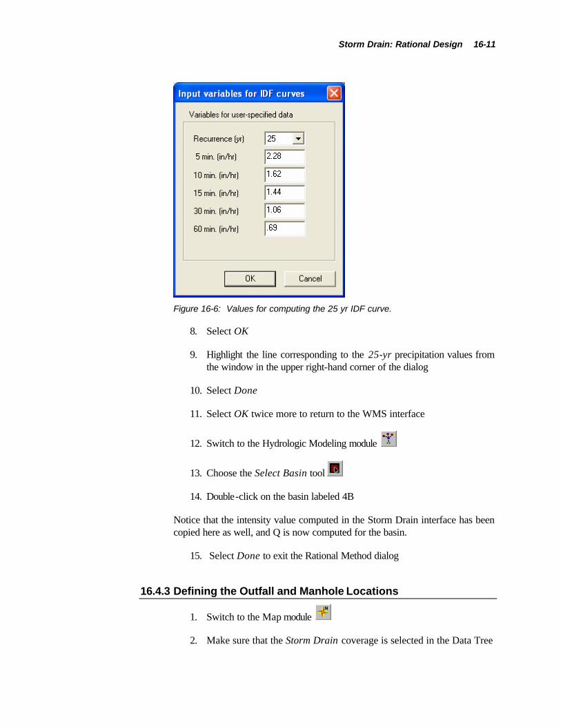
Storm Drain: Rational Design 16-11
Figure 16-6: Values for computing the 25 yr IDF curve.
8. Select OK
9. Highlight the line corresponding to the 25-yr precipitation values from the window in the upper right-hand corner of the dialog
10. Select Done
11. Select OK twice more to return to the WMS interface
12. Switch to the Hydrologic Modeling module
13. Choose the Select Basin tool
14. Double-click on the basin labeled 4B
Notice that the intensity value computed in the Storm Drain interface has been copied here as well, and Q is now computed for the basin.
15. Select Done to exit the Rational Method dialog
16.4.3 Defining the Outfall and Manhole Locations
1. Switch to the Map module
2. Make sure that the Storm Drain coverage is selected in the Data Tree

16-12 WMS Tutorials
3. Choose the Select Feature Point/Node tool
4. Double-click on the node in the lower left-hand corner of the subdivision as shown in Figure 16-7
Figure 16-7: Outfall location.
5. Change the node type to Outfall
6. Select OK
7. Multi-select the nodes indicated in Figure 16-8 by holding down the <SHIFT> key as you select each node

Storm Drain: Rational Design 16-13
Figure 16-8: Manhole locations.
8. Select Feature Objects | Attributes…
9. Change the node type to Manhole
10. Enter 4.0 as the Manhole Width
11. Change the Bench Type to Flat Bench
12. Select OK
The Pipe Drain Network is now defined
16.5 Linking Nodes and Assigning Elevations
To properly portray the relationship between the Drainage coverage and the Storm Drain coverage, we need to explicitly define links between their corresponding nodes. We also need to assign elevations to all linked nodes. Elevations can either be defined manually, or with the use of a background TIN or DEM. We will use the TIN that we opened earlier in this tutorial for assigning elevations.

16-14 WMS Tutorials
1. Select Storm Drain | Link Nodes…
2. Click the Auto Link button. This will link the storm drain inlets from the Drainage coverage to the manholes in the Storm Drain coverage. All nodes should be linked except the one node just upstream of the outfall. This node is a pipe junction and is not associated with a storm drain inlet.
3. Select OK
4. Select Storm Drain | Assign Pipe Elevations. This command automatically assigns elevations to nodes based on an underlying TIN or DEM, if one is present.
With Drainage and Storm Drain nodes linked together and elevations assigned to our pipe network, we are ready to save the Storm Drain model.
16.6 Saving the Simulation and Running Storm Drain
1. Select File | Save As…
2. Make sure the Save as type filter is set to WMS Project Files (*.wpr)
3. Enter wms_storm_rat for the File name
4. Select Save
5. Select Storm Drain | Save Simulation
6. Save the file as wms_st_r
7. Select Storm Drain | Run Simulation
8. Verify that the input file name is “wms_st_r.hda”
9. Change the output file name to “wms_st_r.lst”
The input and output file name prefixes can be up to 8 characters in length. If you enter an input file name longer than 8 characters, Storm Drain will not run. If you enter an output file name longer than 8 characters, it is truncated to 8 characters when Storm Drain writes the file. Also all directory names in the path of the input/output files cannot contain more than 8 charcters.
10. Select OK

Storm Drain: Rational Design 16-15
11. Once Storm Drain (HYDRA) has finished running, select Close
12. Select File | Edit File…
13. Open “wms_st_r.lst”
14. Select OK to open the file with Notepad
By browsing through this file , you will see all of the parameters calculated by the Storm Drain (HYDRA) model, such as recommended pipe diameters, pipe invert elevations, flows, velocities, and hydraulic grade line computations.
15. Close Notepad


17 Storm Drain: Hydrographic Design
CHAPTER 17
Storm Drain: Hydrographic Design
Storm Drain is a hydraulic analysis and design program for storm drain and sanitary sewer systems. It was developed by the Federal Highway Administration with the intent of providing hydraulic engineers a quick and accurate method of designing and analyzing storm drain, sanitary sewer, and combination systems. The Storm Drain interface in WMS uses the same HYDRA program to perform calculations that is currently part of the FHWA’s HYDRAIN suite of hydraulic programs.
This tutorial demonstrates how to use WMS to set up a Hydrographic Drainage simulation for use with Storm Drain. We will set up drainage areas and Runoff Coefficients for a subdivision, similar to the one in the previous tutorial, but this time we will also specify gutter locations in the Drainage coverage. As illustrated in this tutorial, the pipe network does not need to flow parallel or in the same direction as the over-lying drainage. However, there are some limitations in the way the drainage coverage is constructed in order to run a hydrographic analysis with Storm Drain. The most important thing is that each inflow hydrograph needs to be associated with one and only one gutter at the storm drain inlet. In other words “extra” stream arcs that are not part of the gutter leading into the inlet should be deleted.
In this analysis we will generate input hydrographs using the Rational Method calculator, but it should be emphasized that any hydrologic method that produces a hydrograph can be used, or hydrographs may be entered manually.
17-2 WMS Tutorials
17.1 Objectives
In this tutorial, we will set up a hydrographic storm drain simulation for a hypothetical subdivision. The objective of this tutorial is to teach you the basic steps for defining a Storm Drain input file for hydrographic analysis. These steps include the following:
1. Build the drainage basins and make adjustments for limitations in doing a hydrographic analysis
2. Perform a simple Rational Method analysis to generate input hydrographs
3. Digitize a small pipe network based on the surface drainage
4. Define the necessary parameters for the pipe network
5. Run Storm Drain (HYDRA)
6. View the solution
17.2 Developing the Surface Drainage Coverage
This tutorial will begin with a drainage coverage created with techniques typical to those described in earlier tutorials. In order to prepare the drainage coverage for storm drain analysis we will eliminate all of the stream arcs, except ones that lead into a given outlet (a storm drain inlet in this case). Having extra branching streams does not allow WMS to build the storm drain input file correctly. So you must decide which arc represents the primary stream (in this case a gutter) into an inlet and then delete the others.
1. Switch to the Map module
2. Select File | Open…
3. Open “sdstart.map”
17.2.1 Eliminating Unnecessary Stream Arcs and Nodes
Figure 17-1: Initial drainage coverage with unnecessary stream arcs highlighted.
shows the drainage coverage, with the extra streams highlighted. In order to prepare the drainage coverage correctly you will need to delete these stream arcs.

Storm Drain: Hydrographic Design 17-3
Figure 17-1: Initial drainage coverage with unnecessary stream arcs highlighted.
1. Select the Select Arc tool
2. While holding down the <SHIFT> key (for multi-selection) select the four arcs highlighted in Figure 17-1
3. Select the Delete Macro (or Edit | Delete)
4. Select OK
You must now delete the extra nodes that were at the intersection of the arcs just deleted and the remaining arcs so that there is just a single arc entering the storm drain inlet points.
5. Select the Select Feature Point/Node tool
6. While holding down the <SHIFT> key select the three nodes identified in Figure 17-2 (be sure to select the point to the right of the outlet at the far right and not the point that is the outlet)
Figure 17-2: Nodes that need to be converted to vertices.

17-4 WMS Tutorials
7. Select Feature Objects | Vertex <-> Node
17.2.2 Initializing Storm Drain Simulation
In order to assign the remaining stream arcs to be gutters and the outlet points as storm drain inlets we must initialize a storm drain analysis.
1. Select Storm Drain from the drop down list of models in the Edit window
2. Select Storm Drain | New Simulation
17.2.3 Assigning Stream Arcs as Gutters
1. Select the Select Arc tool
2. While holding down the <SHIFT> key, select all four stream arcs as indicated in Figure 17-3
Figure 17-3: Arcs to be selected.
3. Select Feature Objects | Attributes…
4. Select Gutter for the Feature Arc Type
5. Choose the Atts button to define the properties of the gutters
6. Set the type to Uniform Gutter (should be the default) and set the Manning’s N to 0.015, the Roadway Cross-slope to 0.02, and the width to 2.0
7. Select OK
8. Select OK
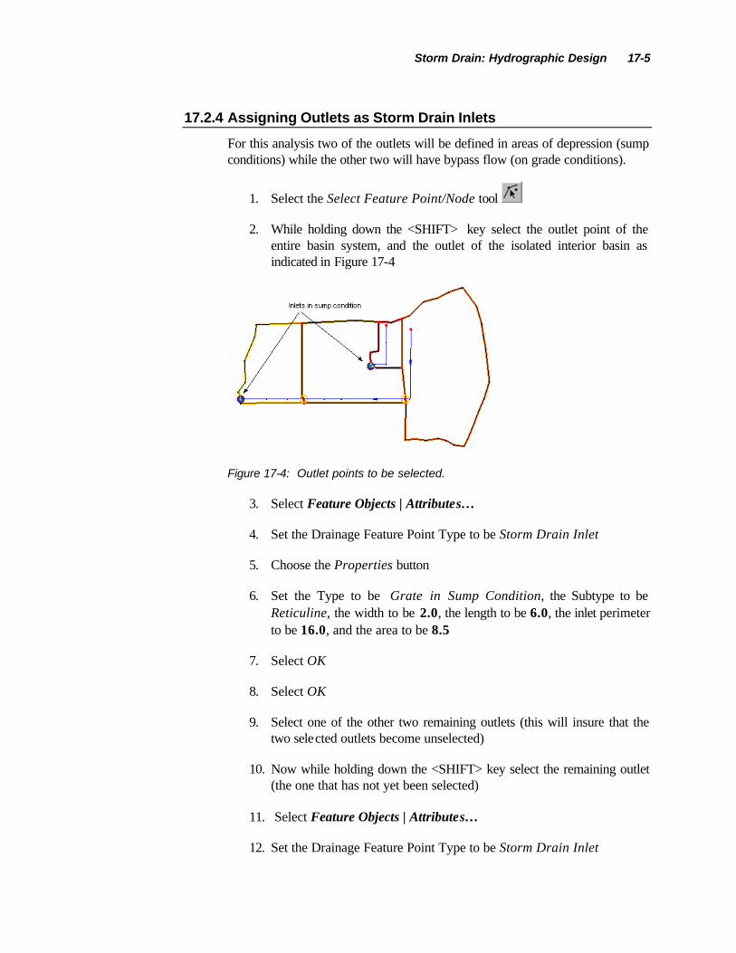
Storm Drain: Hydrographic Design 17-5
17.2.4 Assigning Outlets as Storm Drain Inlets
For this analysis two of the outlets will be defined in areas of depression (sump conditions) while the other two will have bypass flow (on grade conditions).
1. Select the Select Feature Point/Node tool
2. While holding down the <SHIFT> key select the outlet point of the entire basin system, and the outlet of the isolated interior basin as indicated in Figure 17-4
Figure 17-4: Outlet points to be selected.
3. Select Feature Objects | Attributes…
4. Set the Drainage Feature Point Type to be Storm Drain Inlet
5. Choose the Properties button
6. Set the Type to be Grate in Sump Condition, the Subtype to be Reticuline, the width to be 2.0, the length to be 6.0, the inlet perimeter to be 16.0, and the area to be 8.5
7. Select OK
8. Select OK
9. Select one of the other two remaining outlets (this will insure that the two selected outlets become unselected)
10. Now while holding down the <SHIFT> key select the remaining outlet (the one that has not yet been selected)
11. Select Feature Objects | Attributes…
12. Set the Drainage Feature Point Type to be Storm Drain Inlet

17-6 WMS Tutorials
13. Choose the Properties button
14. Set the Type to be Grate on grade, the Subtype to be Reticuline, the width to be 2.0, and the length to be 6.0
15. Select OK
16. Select OK
17. Select Feature Objects | Compute Basin Data…
18. Select OK
17.3 Running a Rational Analysis
We will perform a simple Rational analysis of this subdivision and use the Rational method hydrographs as input for the hydrographic storm drain analysis. You should remember though that any of the hydrologic analysis models in WMS can be used, or input hydrographs may be entered manually.
1. Select the Hydrologic Modeling module
2. Change the Model drop-down box located at the top of the WMS interface to Rational
17.3.1 Defining Rational Method Basin Parameters
1. Double-click on one of the basin icons using the Select Basin tool and defined the basin parameters according to Figure 17-5 and Table 17-1. Select another basin and define its parameters until all basin data is defined. For more details on defining a Rational Simulation see the tutorial on Rational method analysis.

Storm Drain: Hydrographic Design 17-7
Figure 17-5: Basin locations.
Table 17-1: Rational Method basin parameters.
Basin C I (in/hr) Tc (min) 1 .1 2.4 22 2 .15 2.7 18 3 .15 3.1 12 4 .2 3.8 7
2. Select Done in the Rational Method dialog
17.3.2 Defining Rational Method Routing Parameters
1. Define the intensity and routing time (where not dimmed) for the four confluence points connected to the basins according to Table 17-2. As with basins, reach data are entered by double -clicking on the yellow
outlet icons using the Select Outlet tool .
Table 17-2: Rational Method routing parameters.
Outlet Routing Lag (min) I (in/hr) 1 5 2.4 2 4 1.9 3 -- 1.7 4 -- 3.8
2. Select Done in the Rational Method dialog
17.3.3 Computing Hydrographs
1. Double-click on the outlet for the isolated interior basin (the outlet of basin 4 in Figure 17-5

17-8 WMS Tutorials
2. Choose the Define Hydrographs button
3. Select Done (use the default settings for the Rational hydrograph method)
4. Select Done
5. Double-click on the outlet for the entire watershed (the outlet of basin 3 in Figure 17-5)
6. Choose the Define Hydrographs button
7. Select Done (use the default settings for the Rational hydrograph method)
8. Select Done
At this point you should have hydrographs defined for the drainage coverage. These hydrographs will be used as input to the storm drain problem.
17.4 Creating the Pipe Network
You will now create a storm drain pipe network that connects the isolated interior basin to the others and exits west of the watershed outlet. You will do this by creating a Storm Drain coverage and then digitizing the storm drain pipes
using the Create Feature Arc tool .
17.4.1 Digitizing Storm Drain Pipes
1. Switch to the Map module
2. Expand the Map Data folder in the Data Tree (if it isn’t already expanded)
3. Right-click on the Map Data folder in the Data Tree window
4. Select New Coverage
5. Change the Coverage type to Storm Drain
6. Select OK
7. Select the Create Feature Arc tool

Storm Drain: Hydrographic Design 17-9
8. Beginning at point just to the left (west) of the outlet of the watershed (basin 3) begin a pipe network segment and end it by double-clicking on top of the outlet of basin 3.
9. Now complete the storm drain network by creating the pipe segments from downstream to upstream between basin 3 and basin 2, basin 2 and basin 1, and a connection from the pipe between basin 2 and basin 1 to the outlet of basin 4. Be sure that feature nodes (segment endings) are created by double-clicking to end the arc to correspond with the storm drain inlets of the drainage coverage. Your storm drain coverage should look like the one in Figure 17-6.
Figure 17-6: View of the Storm Drain coverage.
17.4.2 Entering Storm Drain Parameters
1. Select Storm Drain | Job Control
2. Set the title to: Hydrographic Storm Drain Analysis.
3. Set the Criteria Switch to 3 - Storm (Hydrographic) only
4. Set the timestep to 2
5. Set the Units to English
6. Choose the Pipe Data Properties button
7. Set the values according to Figure 17-7
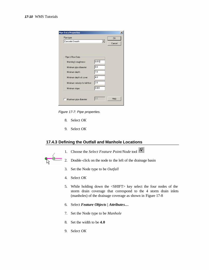
17-10 WMS Tutorials
Figure 17-7: Pipe properties.
8. Select OK
9. Select OK
17.4.3 Defining the Outfall and Manhole Locations
1. Choose the Select Feature Point/Node tool
2. Double-click on the node to the left of the drainage basin
3. Set the Node type to be Outfall
4. Select OK
5. While holding down the <SHIFT> key select the four nodes of the storm drain coverage that correspond to the 4 storm drain inlets (manholes) of the drainage coverage as shown in Figure 17-8
6. Select Feature Objects | Attributes…
7. Set the Node type to be Manhole
8. Set the width to be 4.0
9. Select OK
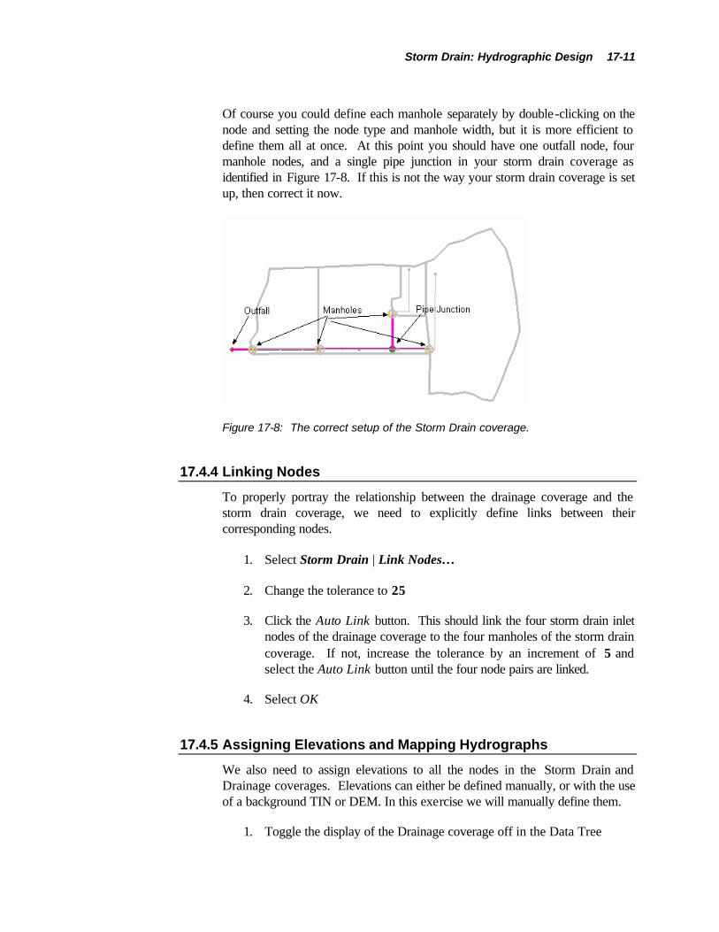
Storm Drain: Hydrographic Design 17-11
Of course you could define each manhole separately by double-clicking on the node and setting the node type and manhole width, but it is more efficient to define them all at once. At this point you should have one outfall node, four manhole nodes, and a single pipe junction in your storm drain coverage as identified in Figure 17-8. If this is not the way your storm drain coverage is set up, then correct it now.
Figure 17-8: The correct setup of the Storm Drain coverage.
17.4.4 Linking Nodes
To properly portray the relationship between the drainage coverage and the storm drain coverage, we need to explicitly define links between their corresponding nodes.
1. Select Storm Drain | Link Nodes…
2. Change the tolerance to 25
3. Click the Auto Link button. This should link the four storm drain inlet nodes of the drainage coverage to the four manholes of the storm drain coverage. If not, increase the tolerance by an increment of 5 and select the Auto Link button until the four node pairs are linked.
4. Select OK
17.4.5 Assigning Elevations and Mapping Hydrographs
We also need to assign elevations to all the nodes in the Storm Drain and Drainage coverages. Elevations can either be defined manually, or with the use of a background TIN or DEM. In this exercise we will manually define them.
1. Toggle the display of the Drainage coverage off in the Data Tree

17-12 WMS Tutorials
2. Choose the Select Feature Point/Node tool
3. Set the elevations of the nodes in the Storm Drain coverage according to the values given in Figure 17-9. To set an elevation select the node and change the elevation in the Z: edit field in the Edit window at the top of the WMS interface.
Figure 17-9: Node elevations for the storm drain pipes.
4. Toggle the Drainage coverage on and the Storm Drain coverage off in the Data Tree
5. Select the Drainage coverage in the Data Tree so that it is the active coverage
6. Set the elevations of all the nodes connected to the gutter arcs according to Figure 17-10
Figure 17-10: Node elevations for the gutters.
7. Toggle the Storm Drain coverage on in the Data Tree and select it so that it is the active coverage
8. Select Storm Drain | Map Hydrographs
With Drainage and Storm Drain nodes linked together and elevations assigned to our pipes and gutters, we are ready to save and run the Storm Drain model.

Storm Drain: Hydrographic Design 17-13
17.5 Saving the Simulation and Running Storm Drain
1. Select File | Save As…
2. Make sure the Save as type filter is set to WMS Project Files (*.wpr)
3. Enter wms_storm_hyd as the File name
4. Select Save
5. Select Storm Drain | Save Simulation
6. Save the file as “wms_st_h”
7. Select Storm Drain | Run Simulation
8. Set the input file name to “wms_st_h.hda” and that the output file name to “wms_sd_h.lst.”
The input and output file name prefixes can be up to 8 characters in length. If you enter a name longer than 8 characters, it is truncated to 8 characters when Storm Drain writes the file. Further no directory in the path to the files can be longer than 8 characters.
9. Select OK
10. Once Storm Drain (HYDRA) has finished running, select Close
11. Select File | Edit File…
12. Open “wms_sd_h.lst”
13. Select OK to open the file with Notepad
By browsing through this file, you will see all of the parameters calculated by the Storm Drain model, such as recommended pipe diameters, pipe invert elevations, flows, velocities, and hydraulic grade line computations.
14. Close Notepad


18 HSPF Interface
CHAPTER 18
HSPF Interface
This chapter demonstrates how WMS can be used to process digital elevation and land use data to develop an HSPF input (.uci) file. The graphical user interface used to define input parameters is demonstrated for a basic hydrology simulation that includes doing the following:
• Delineating watershed segment boundaries from a digital terrain model and USGS land use file.
• Defining segment parameters for a hydrologic analysis.
• Developing reach segment parameters.
• Defining precipitation time series data from standard .wdm database files.
• Entering mass links to define transformations from basin to reach.
18.1 Opening the Watershed and Initializing the HSPF Model
You will open a watershed that has been delineated from a USGS 7.5’ DEM and converted to a TIN.
1. Select File | Open.
2. Locate and choose the file named: littlecotton.wpr. This file should be in the \tutorial\CH18\ directory.

18-2 WMS Tutorials
3. Select OK.
The watershed will appear on your screen with the area displayed in the center of the basin. This indicates that the Basin Data has been computed and you are ready to set up the HSPF model. To initialize the model:
1. Switch to the Tree module .
2. Choose HSPF from the Model drop down list at the Menu bar.
3. Select HSPF | New Simulation.
4. Select HSPF | Global Options.
You will now enter the parameters to indicate that the model will simulate about 3 years of time with a time step of 1 day. You will also name the model, choose the units to use, specify output levels, and name the input/output files:
1. Enter Little Cottonwood Canyon Model in the Title field.
2. Click on the Start Time button; enter Year: 1996, Month: 1, Day: 1, Hour: 0, Minute: 0, Second: 0.0.
3. Click OK; the start date will appear to the right of the Start Time button.
4. Click on the End Time button; enter Year: 1999, Month: 7, Day: 31, Hour: 0, Minute: 0, Second: 0.0.
5. Click OK; the end date will appear to the right of the End Time button.
6. Enter 24 in the hours field under the Time step heading (leave minutes at 0).
7. Ensure that the Units flag is set to English.
8. Change the Run Flag to 1; this indicates that HSPF will interpret the data and run the simulation (0 indicates that HSPF will only interpret – error check- the data).
9. Set the OUTLEV to 10 (under Output Levels); this indicates maximum output to the Error and Warning files. Leave the SPOUT flag at 0 (this is only for Special Actions).

HSPF Interface 18-3
10. In the Files section, enter littleco in the Prefix field, then click the Update Filenames button. This names all the HSPF input/output files associated with this model to the same name.
Note : you have just indicated that you will be using a file named “littleco.wdm” for time series input and output – this file must be created and named appropriately outside of WMS (this has been done for you in this case).
11. Select OK.
The Global Options are now set for your model. You are now ready to proceed to segmenting the watershed and entering parameters for the segments.
18.2 Importing Land Use and Segmenting the Watershed
To divide this watershed into hydrologically similar segments, you will overlay a land-use data layer. You will read this data from an ArcView Shapefile:
1. Select File | Open. Make sure the \tutorial\CH18\ directory is selected.
2. Select the file named littleclanduse.shp and click Open.
3. When the Import Shapefile Data dialog appears, click on the Active Coverage Options button.
4. In the coverage properties dialog, change the coverage type to Land Use.
5. Click OK to return to the Import Shapefile Data dialog; note that the land use coverage is listed by the Active Coverage Options button.
6. Click on the Attribute Mapping button under Polygons. This will allow you to choose the database fields that correspond to WMS attributes.
7. Choose LUCODE in the Database fields window and Land Use in the Coverage attributes window, then click on the Map button. You will see a new line appear in the lower window.
Note : You may get a warning message if LUCODE and Land Use are already mapped. If you do get that warning, click OK and you will see LUCODE=> Land Use line in the lower window.

18-4 WMS Tutorials
8. Choose PERIMETER=> Basin perimeter line in the lower window and click Unmap. This attribute is recognized automatically by WMS, but is not needed in this case.
9. Choose Done.
10. Choose OK in the Import Shapefile Data dialog to read the file.
You will see the land use data polygons overlaid on the watershed. You are now ready to compute HSPF segments based on the land use polygons that fall inside the watershed.
1. Select Calculators | Compute GIS Attributes.
2. Choose HSPF Segments from the Computation drop-down list.
3. In the central section of the dialog, ensure that Land use coverage appears next to “Use a” text and that LC Land Use is the selected Land use coverage name .
4. A text file that correlates the land use id to land use attributes (name, perviousness, etc.) must be read in. Click the Import button to browse for this file. Make sure the \tutorial\CH18\ directory is selected.
5. Choose the file named littleclanduse.tbl. Click Open to read it into WMS.
6. Choose OK in the Compute GIS Attributes dialog to compute the HSPF segments.
7. Click OK when warned that Continuing will delete all HSPF segment data. (If you get that warning)
You should now see the segments computed for the watershed displayed. Each colored area represents a segment to be modeled by HSPF. To better view the segments, you will need to change some display options.
1. Switch to the Map module .
2. Click on the plus sign “+” next to Map Coverages folder in the Data Tree. (If it is minus sign “-“, proceed to the next step)
3. Click the toggle box next to LC Land Use to make it not visible.
4. Select Display | Display Options.
5. Choose the tab entitled General.

HSPF Interface 18-5
6. Toggle ON the Land use legend.
7. Click OK.
You should now see the land use legend which shows the color and title of each segment in the watershed. You may want to Pan and/or Zoom to avoid having the legend appear over the watershed.
18.3 Aggregating Segments
You will note from the display that there are several land segments in the watershed. Some are quite large, such as the Evergreen Forest Land segment, while others are rather insignificant, like Bare Exposed Rock. To make this simulation simpler, you will aggregate some of these segments and delete some others.
1. Switch to the Tree module .
2. Select the basin icon by clicking on it.
3. Select HSPF | Edit Parameters.
4. Note in the Edit Parameters dialog the list of segments in the Basin Data window. There are 8 separate segments (or land use classifications) in this watershed.
There are two ways to reduce the number of segments computed by WMS. The first is to delete one segment, then add the area of the deleted segment, manually, to another similar segment (aggregate segments). The second is to just delete the segment, then let WMS redistribute the deleted area to the remaining segments (Linear distribution).
1. Choose segment entitled Other Urban Or Build Up from the Basin Data window. Note that the area is about 35 acres – insignificant in this watershed.
2. Click the Delete button.
3. Click Yes for the message that asks if the segment is to be removed from further use.
4. Repeat steps 1, 2 and 3 for the segment entitled Bare Ground.
5. Click Done.
6. Switch to the Drainage module .

18-6 WMS Tutorials
7. Select TIN | Compute Basin Data. Click OK on the Compute Basin Data dialog to proceed. This will re-compute basin data and distribute the deleted segments’ areas to the remaining segments.
8. Now you will aggregate some segments. Switch back to the Tree module .
9. Select the basin icon by clicking on it.
10. Select HSPF | Edit Parameters. Note that there are only 6 segments listed now.
11. Choose the segment entitled Mixed Forest. Note the area of 474.94 acres; this is the area that you will add to the Evergreen Forest segment to aggregate the two segments.
12. While highlighting Mixed Forest segment, change its area to 0.0 (from 474.94).
13. Click the Delete button to delete segment 6.
14. Click Yes to confirm removing the segment.
15. Choose Evergreen Forest segment. Note the area is 12237.15 acres.
16. Enter the new Area = 12712.1 acres (12237.15 + 474.94). You have successfully aggregated two segments.
17. Aggregate segments by setting the Bare Exposed Rock segment area to 0.0, deleting it, and adding its area to the segment Mixed Tundra. The new total area will be 1444.1acres.
18. Choose Done to exit the Edit Parameters dialog.
You are now left with 4 land segments. These are the segments for which you will now input parameters and simulate with HSPF.
18.4 Defining Land Segment Parameters
You are ready to begin defining parameters for the land segments of the HSPF model. This model will be set up for purely hydrologic analysis; thus, you will be activating and inputting parameters only to the SNOW and WATER modules of HSPF. Further, to decrease the time needed to complete the tutorial, you will fully set up one segment then copy those parameters to the other 3 in the model. Do the following to complete these tasks:
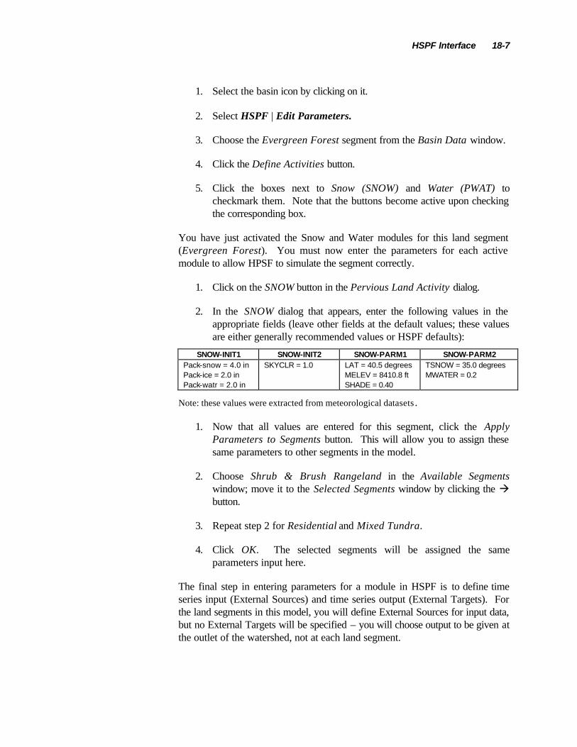
HSPF Interface 18-7
1. Select the basin icon by clicking on it.
2. Select HSPF | Edit Parameters.
3. Choose the Evergreen Forest segment from the Basin Data window.
4. Click the Define Activities button.
5. Click the boxes next to Snow (SNOW) and Water (PWAT) to checkmark them. Note that the buttons become active upon checking the corresponding box.
You have just activated the Snow and Water modules for this land segment (Evergreen Forest). You must now enter the parameters for each active module to allow HPSF to simulate the segment correctly.
1. Click on the SNOW button in the Pervious Land Activity dialog.
2. In the SNOW dialog that appears, enter the following values in the appropriate fields (leave other fields at the default values; these values are either generally recommended values or HSPF defaults):
SNOW-INIT1 SNOW-INIT2 SNOW-PARM1 SNOW-PARM2 Pack-snow = 4.0 in Pack-ice = 2.0 in Pack-watr = 2.0 in
SKYCLR = 1.0 LAT = 40.5 degrees MELEV = 8410.8 ft SHADE = 0.40
TSNOW = 35.0 degrees MWATER = 0.2
Note: these values were extracted from meteorological datasets .
1. Now that all values are entered for this segment, click the Apply Parameters to Segments button. This will allow you to assign these same parameters to other segments in the model.
2. Choose Shrub & Brush Rangeland in the Available Segments window; move it to the Selected Segments window by clicking the à button.
3. Repeat step 2 for Residential and Mixed Tundra.
4. Click OK. The selected segments will be assigned the same parameters input here.
The final step in entering parameters for a module in HSPF is to define time series input (External Sources) and time series output (External Targets). For the land segments in this model, you will define External Sources for input data, but no External Targets will be specified – you will choose output to be given at the outlet of the watershed, not at each land segment.

18-8 WMS Tutorials
1. Click on the External Sources button in the SNOW dialog. The Assign External Sources dialog will appear with a list of the datasets available in the WDM file specified for this model (littleco.wdm).
2. If there is nothing in there (and you might also get a warning message that the file is not there), Open the littleco.wdm file and click OK.
3. Assign the following datasets as sources by setting the fields to the appropriate values, then clicking the Assign button for each line. If you make a mistake, choose the incorrect line in the lower window and click Delete.
Member Name
Member subscrip
t
Units Missing Data
Transformation Quality flag
Multiplication Factor
Dataset
PREC ENGL UNDF SAME 0 0.25 3 PREC ENGL UNDF SAME 0 0.75 7 DTMPG ENGL UNDF AVER 0 1.0 14 WINMOV ENGL UNDF AVER 0 1.0 15 SOLRAD ENGL UNDF SAME 0 1.0 16 AIRTMP ENGL UNDF AVER 0 0.4 17 AIRTMP ENGL UNDF AVER 0 0.6 18
1. Since you will add other External Sources to this segment with the PWAT module input, you will not assign the External Sources to other segments yet. Click Done to return to the SNOW dialog.
2. Click OK to return to the Pervious Land Activities dialog.
You have completed the set up of the SNOW module. You will now repeat the same basic steps to set up the PWAT module for the land segments of the model.
1. Click on the PWAT button in the Pervious Land Activity dialog.
2. In the PWATER dialog that appears, enter the following values in the appropriate fields (leave other fields at the default values):
PWAT-PARM1 PWAT-PARM2 PWAT-PARM3 PWAT-PARM4
PWAT-PARM5
PWAT-STATE1
CSNOFG = On RTOPFG = On UZFG = On
LZSN = 5.0 INFILT = 0.48 LSUR = 2258.0 SLSUR = 0.25 KVARY = 0.7 AGWRC = 0.997
DEEPFR = 0.1 PETMAX = 35.0 PETMIN = 30.0
CEPSC = 0.1 UZSN = 1.0 NSUR = 0.25 INTFW = 3.0 IRC = 0.7 LZETP = 0.8
CEPS = 0.2 UZS = 1.0 LZS = 6.0 AGWS = 1.6 GWVS = 1.9

HSPF Interface 18-9
1. Now that all values are entered for this segment, click the Apply Parameters to Segments button. This will allow you to assign these same parameters to other segments in the model.
2. Choose Shrub & Brush Rangeland in the Available Segments window; move it to the Selected Segments window by clicking the à button.
3. Repeat step 2 for Residential and Mixed Tundra.
4. Click OK. The selected segments will be assigned the same parameters input here.
Now you must define the additional External Sources needed for the PWATER simulation. Most of the External Sources entered for the SNOW module are also used for the PWATER module, but there is one input series that is not yet entered.
1. Click on the External Sources button in the PWATER dialog. The Assign External Sources dialog will appear with the sources that you created for this segment in the SNOW module listed in the lower window.
2. Assign the following dataset (evapotranspiration) as a source by setting the fields to the appropriate values, then clicking the Assign button. If you make a mistake, choose the incorrect line in the lower window and click Delete.
Member Name
Member subscript
Units Missing Data
Transformation
Quality flag
Multiplication Factor
Dataset
PETINP ENGL UNDF SAME 0 1.0 23
All the External Sources needed for the simulation are now assigned to this segment. You will now copy these same External Sources to all other land segments in the model.
1. Click the Apply Sources to Segments button. This will allow you to assign these same External Sources to other segments in the model.
2. Choose Shrub & Brush Rangeland in the Available Segments window; move it to the Selected Segments window by clicking the à button.
3. Repeat step 2 for Residential and Mixed Tundra.

18-10 WMS Tutorials
4. Click OK.
5. Click Done in the Assign External Sources dialog.
6. Click OK in the PWATER dialog.
7. Click OK in the Pervious Land Activities dialog.
The Edit Parameters dialog should now be active. You have successfully set up the SNOW and PWATER modules for all land segments in the model (remember that you set up the modules explicitly for the Evergreen Forest segment and then copied the parameters to all other segments). You may want to ensure/review the set up for the other segments by choosing the segment in the Basin Data window, then clicking the Define Activities button and reviewing the SNOW and PWATER input.
Now that the land segment data is complete, you will enter data for the reach (stream) segment of the model.
1. Click Done to close the Edit Parameters dialog.
18.5 Defining Reach Segment Parameters
To simulate runoff in-stream, you will need to activate the HYDR module for the reach segment of the model. You will also need to specify the output dataset needed (a hydrograph in this case) to view the results of the simulation.
1. Double-click on the watershed outlet in the Graphics Window (this can be done while the Edit Parameters dialog is still present by only single-clicking the outlet). The Reach/Reservoir Data section of the Edit Parameters dialog will become active and display the name of the outlet chosen (Little).
2. Click on the Define Activities button.
3. Check the box to activate the Hydraulics (HYDR) module of HSPF for this reach.
4. Click the HYDR button in the Reach/Reservoir Activities dialog.
5. In the HYDR dialog that appears, enter the following values in the appropriate fields (leave other fields at the default values):
HYDR-PARM1 HYDR-PARM2 HYDR-INIT ODFVFG = 4 Length = 13.82
DeltaH = 2200.0

HSPF Interface 18-11
The next input you must enter is the FTABLE for the reach. The FTABLE is a spreadsheet-like table that contain the conveyance parameters of the reach (depth, area, volume, and outflow). This table may be calculated manually or with the help of the Channel Calculator in WMS.
1. Click on the Define FTABLE button the HYDR dialog.
2. In the FTABLE dialog that appears, enter the following values (it is possible to change the number of rows and columns in the FTABLE, but the default values will be sufficient in this case. These values are saved in a text file called ftable.txt in the CH18 directory of the tutorials. You can open this file, copy the data (use CTRL-C to copy), and paste the data to the FTABLE dialog (use CTRL-V to paste) if you wish):
Depth (ft) Area (ac) Volume (ac-ft)
Outflow (cfs)
0.0 0.0 0.0 0.0 0.25 25.99 6.393 13.876 0.5 26.828 12.995 43.954 0.75 27.666 19.807 86.269 1.0 25.50 26.828 139.241 1.25 29.340 34.059 201.950 1.5 30.181 41.499 273.794 1.75 31.019 49.150 354.355 2.0 31.858 57.009 443.334 2.25 35.211 90.540 879.902
1. Click OK to save the FTABLE.
The final task in defining the reach parameters is to specify the output you want to see from the reach and where HSPF will write the output. This is done by defining an External Target. You will specify that you want a hydrograph to be output to a dataset in the WDM (littleco.wdm) file for this reach.
1. Click on the External Targets button in the HYDR dialog.
2. Set the following fields to the specified values:
Member Name
Member subscr ip
t
Units Access
Aggregation
Multiplication Factor
Quality flag
Transformation Function
RO ENGL REPL Aggregate 1.0 0 AVER
1. Select the Use existing dataset button.
2. Click on the Select Dataset button

18-12 WMS Tutorials
3. In the Select Dataset dialog, scroll down and select dataset 20 (Flow), then click the OK button.
4. The Dataset name, type, and number should appear in the Assign External Targets dialog.
5. Click Assign to add the External Target line to the lower window.
6. Click Done.
You have now completed the input for the HYDR module in this reach. This will be the only module active for this simulation; thus, you can exit the parameter editing dialogs.
1. Click OK in the HYDR dialog.
2. Click OK in the Reach/Reservoir Activity dialog.
3. Click Done in the Edit Parameters dialog.
The input for all land and reach segments is now complete in the model. The last task before saving and running the HSPF model is to assign Mass Links.
18.6 Creating Mass Links
Mass Links control how materials (water, sediment, constituents) are transferred from land segments to reaches, and from one reach to the next. Conversions in units, such as inches/acre per day of runoff à cubic feet per second, are defined in the Mass Links also. You will enter Mass Links to transfer water from land to reach and from reach to reach for this model.
1. Select HSPF | Mass Link Editor.
2. When you enter the Mass Link Editor, it is set to begin adding/deleting mass links for PERLND segments. Set the fields to the values below:
Volume Name
Volume Group
Volume Member Name
Multiplication Factor
Target Name
Target Group
Target Member Name
PERLND PWATER PERO 0.083333333 RCHRES INFLOW IVOL
Note: 0.0833333 is the conversion for inches/acre per day à cfs.
1. Click Add Link (if you make a mistake, select the link in the window and click the Delete Link button).
2. Change the Segment Type (upper left) to IMPLND.

HSPF Interface 18-13
3. Set the fields to the values below:
Volume Name
Volume Group
Volume Member Name
Multiplication Factor
Target Name
Target Group
Target Member Name
IMPLND IWATER SURO 0.083333333 RCHRES INFLOW IVOL
1. Click Add Link.
2. Change the Segment Type (upper left) to RCHRES.
3. Set the fields to the values below:
Volume Name
Volume Group
Volume Member Name
Multiplication Factor
Target Name
Target Group
Target Member Name
RCHRES HYDR ROVOL 1.00 RCHRES INFLOW IVOL
1. Click Add Link.
The Mass Links needed for PERLND, IMPLND, and RCHRES segments are now set up. You are ready to save and run the model.
Click OK to exit the Mass Link Editor.
18.7 Saving and Running HSPF Simulation
The last step is to save and run the HSPF simulation.
1. Select HSPF | Run Simulation.
15. HSPF should run to completion. You will then be able to view the solution.


19 HEC-RAS Managing Cross Sections
CHAPTER 19
HEC-RAS - Managing Cross Sections
HEC-RAS is a 1-D river model that relies on cross section data along reaches to compute results. Cross sections can be extracted from a TIN in WMS, but the TIN does not always define the channel with enough resolution to get an accurate cross section through the channel. Tools in WMS make it possible to manage cross sections by editing their shape, defining properties, and merging multiple cross sections together. Surveyed channel cross section data can be merged with cross sections extracted from a TIN in order to develop cross sections that accurately depict both the channel and surrounding terrain.
19.1 Objectives
In this tutorial you will learn how to merge cross sections and use the data for input into a HEC-RAS model by:
1. Creating a conceptual river model
2. Converting a DEM to a TIN for background elevation data
3. Extracting cross sections
4. Merging cross sections
5. Running HEC-RAS
6. Delineating the floodplain using HEC-RAS results

19-2 WMS Tutorials
19.2 Creating a Conceptual River Model
A conceptual river model can be created by using GIS data to define centerline and bank arcs, material properties, and cross section location and geometry. Background images are also useful in creating and viewing this GIS data.
19.2.1 Open Images
1. Switch to the Map module
2. Select File | Open…
3. Open “jordannarrows.jpg”and “midvale.jpg”
19.2.2 Define Centerline and Bank Arcs
1. Select File | Open…
2. Open “river.map”
3. Zoom in close enough around a section of the feature arcs so that you can see three distinct arcs as shown in Figure 19-1
Figure 19-1: Centerline and bank arcs.
The middle arc is the centerline arc that defines the thalweg of the river reach and the outer arcs define the right and left banks.

HEC-RAS - Cross Section Management 19-3
4. Use the Select Feature Arc tool to select the middle arc
5. Select Feature Objects | Attributes… and choose Centerline
6. Select OK
7. Enter Jordan River for the River Name
8. Enter Riverton in the Reach Name
9. Select OK
10. Use the Select Feature Arc tool to select both outer arcs
11. Select Feature Objects | Attributes… and choose Bank
12. Select OK
19.2.3 Create Materials
Materials are defined on an Area Property coverage by digitizing polygons representing different materials using a background image, such as an aerial photograph, or by using land use data from a shapefile or another source. Each different material that is defined will be used later to assign roughness values to the cross sections. In this tutorial we will read in a *.map file containing material data that has already been digitized.
1. Select File | Open…
2. Open “materials.map”
3. Zoom in around the materials polygons on the Area Property coverage
4. Select Display | Display Options…
5. Toggle Color Fill Polygons on
6. Select OK
7. Select Edit | Materials… to view the material types associated with each color
8. Select Cancel

19-4 WMS Tutorials
19.3 Converting a DEM to a TIN
Cross section geometry can be extracted from a TIN in WMS. We will create a TIN by opening a DEM and converting it to a TIN. It is also possible to filter redundant DEM points out of the TIN that we create.
19.3.1 Open DEM
1. Switch to the Terrain Data module
2. Select File | Open…
3. Open “91606647.hdr”
4. Select OK
5. Select Yes to convert coordinates
6. Toggle Edit project coordinate system on
7. Set the Convert From Horizontal System to Geographic NAD 83 (US)
8. Set the Convert To Horizontal System to UTM NAD 27 (US)
9. Select OK
19.3.2 Convert to a TIN
1. Select DEM | Conversion | DEM->TIN | Filtered…
2. Select OK
3. Select Display | Display Options…
4. Toggle Triangles off and Boundaries on
5. Select OK
6. Expand the Terrain Data folder in the Data Tree
7. Hide the DEM by toggling its checkbox off

HEC-RAS - Cross Section Management 19-5
19.4 Extracting Cross Sections
It is very easy to extract cross section geometry from a TIN in WMS. This is done by creating arcs that represent the plan view of the cross sections on a 1-D Hyd Cross Section coverage.
1. Switch to the Map module
2. Select File | Open…
3. Open “xsections.map”
4. Zoom in around the cross section arcs labeled 0 - 4
5. Hide the materials polygons by toggling Area Property coverage in the Data Tree off
6. Hide the background images by toggling them off
7. Select Display | Contour Options…
8. Select the Specified interval option and enter a value of 10.0
9. Select OK
You can see that the cross section arcs are approximately as wide as the floodplain might be. They end where there is a sharp break in slope and the terrain gets relatively steep. Wider cross section arcs are generally not necessary for a HEC-RAS analysis.
10. Make sure the 1D-Hyd Cross Section coverage is active in the Data Tree
11. In the Model drop-down list at the top of the screen select River Tools
12. Select River Tools | Extract Cross Section…
13. Select OK
14. Enter xsec for the name of the new cross section database where all of the cross sections will be stored

19-6 WMS Tutorials
19.5 Merging cross sections
Any two cross sections can easily be merged in WMS. We will create a new cross section database that stores surveyed channel cross section data and merge that with the cross sections that we just extracted from the TIN. Merging cross sections will create more accurate cross section geometry data. Cross sections are merged by aligning both cross sections using reference points such as the thalweg or bank locations and then inserting points from one cross section into the other.
19.5.1 Open channel cross section data
1. Select File | Edit File…
2. Open “channel.txt”
3. Select OK to open with Notepad or choose any other text editor or spreadsheet
19.5.2 Create a new cross section database
1. Select River Tools | Manage Cross Sections…
2. Choose the New Cross Section Database… button
3. Enter channelxsec for the File name
4. Select Save
19.5.3 Define channel cross sections in the database
The current cross section database should be “channelxsec.idx” (the one that you just created).
1. Click on the Edit Cross Section Database… button
2. Click the New button to add a cross section to the database
3. Select the Edit button to edit the cross section
4. Click the Add button and enter 7 to add 7 points to the cross section
5. Select OK
6. Toggle XY off

HEC-RAS - Cross Section Management 19-7
7. Copy and paste the cross section data for Channel Section 1 from “channel.txt” (opened in Notepad) into the Cross-Section Attributes Geom Edit tab as shown in Figure 19-2. Make sure to paste the data into the first row.
Figure 19-2: Adding cross section geometry data to the database.
8. Choose the Point Props tab
9. Click the Auto Mark button to automatically define thalweg and right/left bank points. These reference points will be used to align cross sections for merging.
10. Select OK

19-8 WMS Tutorials
11. Repeat steps 2-10 to add the 4 remaining channel cross sections in “channel.txt” to the cross section database
12. Click the Save button
13. Select OK
14. Select OK
19.5.4 Align channel cross sections with extracted cross sections
1. Use the Select Feature Arc tool to select the cross section arc at the
top of the screen labeled 0
2. Select Feature Objects | Attributes…
3. Select Assign Xsec
This will allow you to view all of the extracted cross sections and assign the highlighted geometry to this cross section arc.
4. Click the Edit button
5. Select the Line Props tab to view the material properties (roughness values) that will be applied to each cross section. These can be edited if necessary.
6. Select the Merge tab
7. Select the Load Insert Cs button
8. Click on the Data Base Browse button
9. Open “channelxsec.idx”
10. Make sure that the csid number that is highlighted for the channel cross section matches the csid number of the extracted cross section that you are editing (these numbers also match the number labels displayed next to each cross section arc on the screen)
11. Select OK
You will see a profile of the surveyed cross section geometry appear in the upper left corner of the profile view of the extracted cross section geometry as shown in Figure 19-3.

HEC-RAS - Cross Section Management 19-9
Figure 19-3: Merging cross sections.
Merge cross sections using the Alignment tools shown in Figure 19-4. You can align cross sections using reference points (point properties) that are defined on both cross sections such as left end, left bank, thalweg, right bank, and right end. Enter a value for the Offset the and cross section will be offset that distance from the alignment point. Specify a distance for Step Z and use the Up and Down buttons to move the inserted cross section vertically. Do the same for Step D using the Left and Right buttons to move the cross section horizontally. The horizontal and vertical scales on the plots are useful for determining the distances to enter. (Remember that the scales are not equal and so the vertical distances are magnified)

19-10 WMS Tutorials
Figure 19-4: Alignment tools.
12. Choose Thalweg for Alignment to align the thalweg (specified as a point property) of the channel cross section with the thalweg of the extracted cross section
13. Enter a value for Step Z (try 5) and use the Down button to move the channel cross section vertically
14. Reduce the Step Z value to 1 and use the Up button to position the cross section
15. Keep reducing the Step Z value and using the Up and Down buttons until the cross sections are aligned correctly
16. Enter a value for Step D and use the Left and Right buttons if you need to move the channel cross section horizontally
The Zoom tool is useful for viewing the alignment of the cross sections close-up once you have the channel cross section located in the general area where it will be inserted.
The aligned should look similar to Figure 19-5:
Figure 19-5: Aligned cross sections.
17. For Merge select Insert All
18. Click Apply to insert the channel cross section and permanently change the extracted cross section data
19. Select OK and notice the updated extracted cross section geometry

HEC-RAS - Cross Section Management 19-11
20. Select OK
21. Select OK
22. Repeat this process (steps 1-21) for all of the cross section arcs
19.6 Running HEC-RAS
A schematic will be created using the GIS data defined in WMS and exported to HEC-RAS. Post-processing options are also available in WMS after running a HEC-RAS simulation.
19.6.1 Creating a schematic and defining roughness values
1. Make the 1D-Hyd Centerline the active coverage in the Data Tree
2. Select River Tools | Map -> 1D Schematic
3. Switch to the River module
4. Select HEC-RAS | Material Properties…
5. Enter roughness values for Agriculture, Brushland, Bare, River, and Urban as shown in Figure 19-6
Figure 19-6: Materials roughness values.
6. Select HEC-RAS | Model Control…
7. Select Materials to use them to generate roughness values

19-12 WMS Tutorials
8. Select OK
19.6.2 Running HEC-RAS
1. Select HEC-RAS | Export GIS File…
2. Enter hecras.geo and Save
This will start HEC-RAS with the geometry file exported from WMS already loaded.
3. Select Options | Unit system (US Customary/SI)…
4. Select System International (Metric System)
5. Select OK
6. Select Yes to set the project units to SI (metric)
7. Select Edit | Geometric Data…
8. Select OK on the Schematic Plot Extents error message
9. Select View | Set Schematic Plot Extents…
10. Click the Set to Computed Extents button
11. Select OK to view the geometric data. It should look similar to the data shown in Figure 19-7
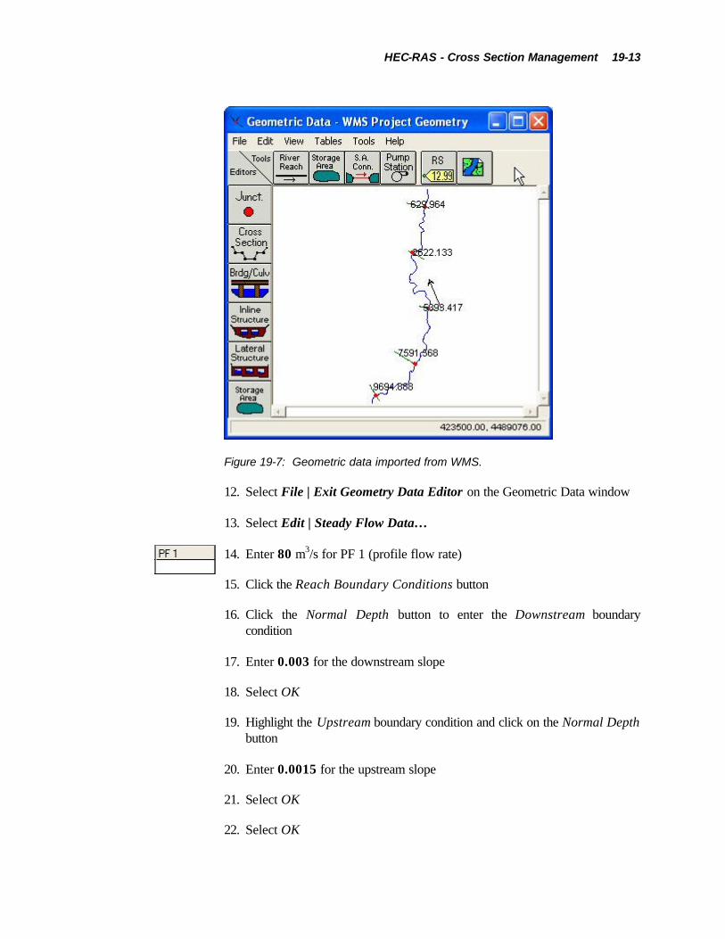
HEC-RAS - Cross Section Management 19-13
Figure 19-7: Geometric data imported from WMS.
12. Select File | Exit Geometry Data Editor on the Geometric Data window
13. Select Edit | Steady Flow Data…
14. Enter 80 m3/s for PF 1 (profile flow rate)
15. Click the Reach Boundary Conditions button
16. Click the Normal Depth button to enter the Downstream boundary condition
17. Enter 0.003 for the downstream slope
18. Select OK
19. Highlight the Upstream boundary condition and click on the Normal Depth button
20. Enter 0.0015 for the upstream slope
21. Select OK
22. Select OK
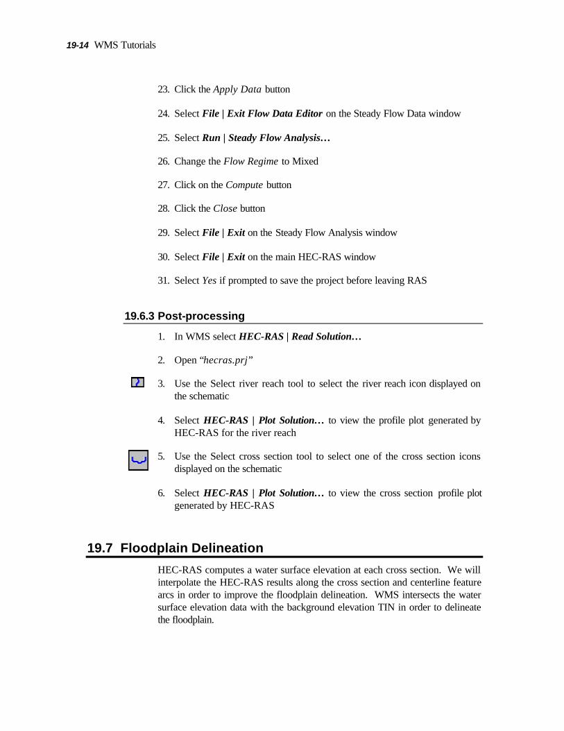
19-14 WMS Tutorials
23. Click the Apply Data button
24. Select File | Exit Flow Data Editor on the Steady Flow Data window
25. Select Run | Steady Flow Analysis…
26. Change the Flow Regime to Mixed
27. Click on the Compute button
28. Click the Close button
29. Select File | Exit on the Steady Flow Analysis window
30. Select File | Exit on the main HEC-RAS window
31. Select Yes if prompted to save the project before leaving RAS
19.6.3 Post-processing
1. In WMS select HEC-RAS | Read Solution…
2. Open “hecras.prj”
3. Use the Select river reach tool to select the river reach icon displayed on the schematic
4. Select HEC-RAS | Plot Solution… to view the profile plot generated by HEC-RAS for the river reach
5. Use the Select cross section tool to select one of the cross section icons displayed on the schematic
6. Select HEC-RAS | Plot Solution… to view the cross section profile plot generated by HEC-RAS
19.7 Floodplain Delineation
HEC-RAS computes a water surface elevation at each cross section. We will interpolate the HEC-RAS results along the cross section and centerline feature arcs in order to improve the floodplain delineation. WMS intersects the water surface elevation data with the background elevation TIN in order to delineate the floodplain.
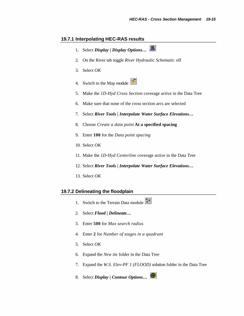
HEC-RAS - Cross Section Management 19-15
19.7.1 Interpolating HEC-RAS results
1. Select Display | Display Options…
2. On the River tab toggle River Hydraulic Schematic off
3. Select OK
4. Switch to the Map module
5. Make the 1D-Hyd Cross Section coverage active in the Data Tree
6. Make sure that none of the cross section arcs are selected
7. Select River Tools | Interpolate Water Surface Elevations…
8. Choose Create a data point At a specified spacing
9. Enter 100 for the Data point spacing
10. Select OK
11. Make the 1D-Hyd Centerline coverage active in the Data Tree
12. Select River Tools | Interpolate Water Surface Elevations…
13. Select OK
19.7.2 Delineating the floodplain
1. Switch to the Terrain Data module
2. Select Flood | Delineate…
3. Enter 500 for Max search radius
4. Enter 2 for Number of stages in a quadrant
5. Select OK
6. Expand the New tin folder in the Data Tree
7. Expand the W.S. Elev-PF 1 (FLOOD) solution folder in the Data Tree
8. Select Display | Contour Options…

19-16 WMS Tutorials
9. For Contour Interval select the Number of contours option and enter 25
10. For Contour Method select Color fill between contours and adjust the Transparency
11. Select OK
Two data sets were created by delineating the floodpla in. W.S. Elev-PF 1_fd contains flood depth values and W.S. Elev-PF 1_wl contains water surface elevations.
12. Select one of the flood delineation data sets and experiment with viewing the results. You may also want to experiment with adjusting the transparency and turn the background image on as shown in Figure 19-8.
Figure 19-8: Flood depth map.
One important thing to remember is that the HEC-RAS results came from merged cross sections, but the floodplain is delineated on the original TIN that does not include the surveyed channel cross section data. The water surface

HEC-RAS - Cross Section Management 19-17
elevations of the flood are the same, but the flood depths in the channels, where cross sections were merged, may be deeper than shown.