This article was downloaded by: [Universite Laval]On: 27 November 2014, At: 07:50Publisher: Taylor & FrancisInforma Ltd Registered in England and Wales Registered Number: 1072954 Registered office: MortimerHouse, 37-41 Mortimer Street, London W1T 3JH, UK

ISH Journal of Hydraulic EngineeringPublication details, including instructions for authors and subscription information:http://www.tandfonline.com/loi/tish20

Water quality based reliability analysis for waterdistribution networksRajesh Gupta a , Sushma Dhapade a , Soumitra Ganguly a & Pramod R. Bhave aa Department of Civil Engineering , Visvesvaraya National Institute of Technology ,Nagpur , IndiaPublished online: 13 Jul 2012.

To cite this article: Rajesh Gupta , Sushma Dhapade , Soumitra Ganguly & Pramod R. Bhave (2012) Water qualitybased reliability analysis for water distribution networks, ISH Journal of Hydraulic Engineering, 18:2, 80-89, DOI:10.1080/09715010.2012.662430

To link to this article: http://dx.doi.org/10.1080/09715010.2012.662430

PLEASE SCROLL DOWN FOR ARTICLE

Taylor & Francis makes every effort to ensure the accuracy of all the information (the “Content”) containedin the publications on our platform. However, Taylor & Francis, our agents, and our licensors make norepresentations or warranties whatsoever as to the accuracy, completeness, or suitability for any purpose ofthe Content. Any opinions and views expressed in this publication are the opinions and views of the authors,and are not the views of or endorsed by Taylor & Francis. The accuracy of the Content should not be reliedupon and should be independently verified with primary sources of information. Taylor and Francis shallnot be liable for any losses, actions, claims, proceedings, demands, costs, expenses, damages, and otherliabilities whatsoever or howsoever caused arising directly or indirectly in connection with, in relation to orarising out of the use of the Content.

This article may be used for research, teaching, and private study purposes. Any substantial or systematicreproduction, redistribution, reselling, loan, sub-licensing, systematic supply, or distribution in anyform to anyone is expressly forbidden. Terms & Conditions of access and use can be found at http://www.tandfonline.com/page/terms-and-conditions

ISH Journal of Hydraulic Engineering

Vol. 18, No. 2, June 2012, 80–89

Water quality based reliability analysis for water distribution networks

Rajesh Gupta*, Sushma Dhapade, Soumitra Ganguly and Pramod R. Bhave

Department of Civil Engineering, Visvesvaraya National Institute of Technology,Nagpur, India

(Received 7 June 2011; final version received 28 August 2011)

The research work in the past two decades on reliability analysis of water distribution networks (WDNs) isprimarily focused on assessing the reliability from the point of view of hydraulics, that is, supplying the requiredquantity of water at the desired pressure, using various qualitative and quantitative measures. A minimumdesired level of residual chlorine at consumer’s tap is needed to supply quality water. In this article, both thequality and quantity of water is taken into account to assess the reliability of a WDN using a ‘water qualityreliability factor’. The water quality reliability factor is defined as the ratio of the total quantity of desired qualityof water supplied by the network to the total quantity of desired quality of water required to be supplied in theperiod of analysis. Pipe-break and pump-failure conditions are considered as random events. Hydraulicsimulation of network under pressure-deficient conditions resulting from pipe-break and pump-failure conditionsis carried out using node flow analysis. The proposed methodology is illustrated with two example networkstaken from the literature.

Keywords: reliability; water distribution networks; water networks; water quality

1. Introduction

The basic objective of any municipal body is to supply safe water in required quantities. Although a lot of research hasbeen done to develop methodologies for reliability analysis based on the supply of an adequate quantity of water, notmuch literature has been available for water quality reliability. Presence of residual chlorine in detectable quantity atconsumer taps ensures water free from bacteriological contamination. However, because of chlorine decay and thecomplexity of water distribution networks (WDNs), it is difficult to ensure just desirable levels of chlorine residual atall times and at all locations. As a practice, higher amounts of chlorine are added at the water source so that chlorineresidual is detected even at the farthest node of the network. Because chlorine reacts with natural organic matter toform undesirable by-products, excessive dosage of chlorine is not desirable. Further, during pipe-failure conditions, theflow pattern in the network changes and residual chlorine may not be available at some of the nodes at the desiredconcentration. How best a network satisfies its objective can be indicated through its water quality reliability.

Reliability can be incorporated in the design of WDNs using either a qualitative or a quantitative criterion. A simplequalitative criterion used traditionally for incorporating reliability in optimal designs of WDNs is the provision of loop-forming links such that they carry some minimum specified discharge or are of some a minimum specified diameter.Loops ensure alternate paths to demand nodes in the event of pipe failure and thus introduce level-one topologicalredundancy. Rowell and Barnes (1982) provided reliability in WDNs by satisfying demand at each node through twoindependent paths from the source. Morgan and Goulter (1985) developed an approach in which the layout of thenetwork is optimally determined such that every node is connected by at least two links. Reliability is betterincorporated in the design of WDNs using a quantitative criterion. Kessler et al. (1990) and Ormsbee and Kessler (1990)considered reliability through the provided level of redundancy, which was defined as the number of simultaneous pipefailures a network can sustain without the supply getting affected at any node either in part or in full. They suggested anoptimisation algorithm in which at least two paths from the source to each demand node, each capable of carrying fullnodal flows, were ensured. Thus, level of redundancy provided was one. Cost of network increases with the providedlevel of redundancy. Even a level-one redundant system may be costly and not affordable. In such a case, a proper levelor reliability is required to be ensured during the design of WDNs. Several other measures of reliability—probability ofpipe breakage (Kettler and Goulter 1985), maximum node isolation probability (Goulter and Coals 1986), probability ofno-node failure (Goulter and Bouchart 1990), system and nodal reliabilities using minimum cut set (Al-Zaharani andSyed 2004; Guercio and Xu 1997; Su et al. 1987), hydraulic availability (Cullinane et al. 1992), the ratio of expectedmaximum flow to total system demand (Fujiwara and De Silva 1990), total volume deficit (Bouchart and Goulter 1991),flow entropy (Awumah et al. 1991; Tanyimboh and Templeman 1993), allowable shortage fraction (Park and Liebman1993), node, volume and network reliability factors using served demands (Agrawal et al. 2007; Gupta and Bhave 1994),capacity reliability (Tolson et al. 2004; Xu and Goulter 1998), network resilience (Devi Prasad and Park 2004)—andapproaches for their evaluation have been suggested in the past two decades (Bhave 2003).

*Corresponding author. Email: drrajeshgupta123@hotmail.com

ISSN 0971–5010 print/ISSN 2164–3040 online

� 2012 Indian Society for Hydraulics

http://dx.doi.org/10.1080/09715010.2012.662430

http://www.tandfonline.com

Dow

nloa

ded

by [

Uni

vers

ite L

aval

] at

07:

50 2

7 N

ovem

ber

2014

However, these approaches include reliability only from hydraulic considerations. Emphasis is now being provided

for supply of a desired quality of water. It is necessary to maintain free chlorine residuals throughout the distributionnetwork between minimum and maximum levels. Several models for prediction of chlorine concentration at different

nodes in a network considering decay of chlorine are developed (Boulos et al. 1995; Rossman et al. 1994). Further,

several studies for number and location of booster stations, and their optimal operations have been suggested with theobjective to minimise the total cost and/or minimise the total chlorine mass to be injected (Boccelli et al. 1998; Kang

and Lansey 2010; Munavalli and Mohan Kumar 2003; Ostfeld and Salomons 2006; Prasad et al. 2004; Tryby et al.

2002). These methodologies are useful in determining the optimal number and location of chlorine booster stations anddeciding their optimal operation schedule under normal working conditions. The present study aims to evaluate the

performance of a WDN in delivering the required quantity of water of desired quality under both normal and pipe-

failure conditions, having known number of booster stations and dose of chlorine injected at various stations. Such ananalysis would be useful in determining the need for additional stations and necessity of adjustment in dose of chlorine.

Ostfeld (2004) defined water quality reliability by the fraction of delivered quality, which is the sum of all time

periods in all simulation (Monte Carlo) runs for which the concentration (any chemical constituent) is below the

threshold concentration factor divided by the total number of simulation runs multiplied by a demand cycle. Kansaland Arora (2004) defined water quality reliability as the proportion of time the network was able to supply a desired

quality of water. Both the above parameters are based on the proportion of time that a network meets water quality.

Kansal and Arora (2004) suggested a methodology for water quality reliability analysis using two parameters—systemhydraulic reliability and system quality reliability. These hydraulic and water quality reliability parameters together

described network reliability. The major drawback in obtaining these parameters was related to modelling

methodology (Gupta et al. 2007). For different pipe-failure conditions, Kansal and Arora (2004) used two-stagemethodology. In the first stage, available nodal heads were obtained using demand-dependent analysis (nodal

outflow¼ demand) and in the second stage, supply at pressure-deficient nodes was reduced using parabolic head-

discharge relationship. This, however, violated the flow continuity relationships at demand nodes. Further, even

though the outflows at nodes were reduced, its effect in predicting chlorine concentration was not accounted for.In this paper, a new parameter and methodology for assessing water quality reliability of WDN is proposed, and

the network is modelled for pressure-deficient conditions using node flow analysis (NFA; Bhave 1981; Bhave and

Gupta 2006; Gupta and Bhave 1996b). The proposed methodology is applied to two example networks.

2. Water quality reliability parameter

An ideal reliability parameter should have some physical meaning, should be able to clearly distinguish different

network conditions and should be easy to calculate. Considering the same, a new water quality reliability parameter is

proposed that is based on the proportion of quantity of water supplied with desired quality. It takes into account bothhydraulic as well as water quality requirements. The water quality reliability parameter is defined as the ratio of the

total quantity of water supplied with desired quality in the period of analysis to the total quantity of water of the

desired quality required in the period of analysis. Thus, water quality reliability, RWQ, is

RWQ ¼

Ps

Pj bjsq

avljs tsP

s

Pj q

reqjs ts

ð1Þ

in which, qavls ¼ available discharge rate during state s; qreqs ¼ required discharge rate during state s; bjs¼ 1 or 0,

depending upon whether the water quality criteria at the demand node is satisfied or not; ts¼ time for the state;j¼ subscript denoting demand node and s¼ subscript denoting state, which is a time period in which the hydraulic

conditions of the network remains same.The available nodal flows during a state are obtained using NFA as described in the next section. The time for any

state, ts, depends on failure rates of pipes and pumps and their repair time. The pipe failure rate depends on severalfactors, which includes pipe material, length and diameter of pipe, soil conditions, previous breaks in the pipe etc. Even

though pipe breaks depend on several factors, here these are considered as a function of diameter only (Goulter and

Coals 1986; Gupta and Bhave 1994; Kettler and Goulter 1985). The break rate increases as the pipe size decreases.Further, it is assumed that 2 days are required for identifying the location of a pipe break, isolating and repairing the

pipeline and resuming water supply (Fujiwara and De Silva 1990; Gupta and Bhave 1994). Thus, time for closure, Tr,

of pipe for one repair is 2 days.Let pð yÞ be the working-condition probability and �pð yÞ be the shutdown probability of a pipe in year y. Using the

break rate N(y) km–1yr–1 for the yth year, these values for a pipe of length L km for year y can be obtained as:

�pð yÞ ¼ ½Nð yÞ � L� ð2Þ

pð yÞ ¼ 1� �pð yÞ ð3Þ

ISH Journal of Hydraulic Engineering 81

Dow

nloa

ded

by [

Uni

vers

ite L

aval

] at

07:

50 2

7 N

ovem

ber

2014

Using working condition and shut down probability and time of closure, the closure and working times (in days)per year for that condition are

Closure time ðin daysÞ per year ¼ Nð yÞ � L� Tr ð4Þ

Working time ðin daysÞ per year ¼ 365�Nð yÞ � L� Tr ð5Þ

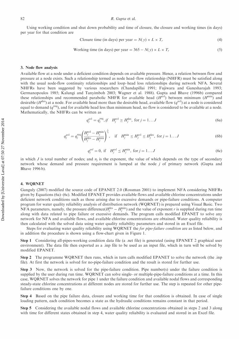
3. Node flow analysis

Available flow at a node under a deficient condition depends on available pressure. Hence, a relation between flow andpressure at a node exists. Such a relationship termed as node head–flow relationship (NHFR) must be satisfied alongwith the usual node-flow continuity relationships and loop–head loss relationships during network NFA. SeveralNHFRs have been suggested by various researchers (Chandapillai 1991; Fujiwara and Ganesharajah 1993;Germanopoulos 1985; Kalungi and Tanyimboh 2003; Wagner et al. 1988). Gupta and Bhave (1996b) comparedthese relationships and recommended parabolic NHFR for available head (Havl) between minimum (Hmin) anddesirable (Hdes) at a node. For available head more than the desirable head, available flow (qavl) at a node is consideredequal to demand (qreq), and for available head less than minimum head, no flow is considered to be available at a node.Mathematically, the NHFRs can be written as

qavlj ¼ qreqj , if Havlj � Hdes

j , for j ¼ 1. . . J ð6aÞ

qavlj ¼ qreqj

Havlj �Hmin

j

Hdesj �Hmin

j

! 1nj

, if Hminj � Havl

j � Hdesj , for j ¼ 1. . . J ð6bÞ

qavlj ¼ 0, if Havlj � Hmin

j , for j ¼ 1. . . J ð6cÞ

in which J is total number of nodes; and nj is the exponent, the value of which depends on the type of secondarynetwork whose demand and pressure requirement is lumped at the node j of primary network (Gupta andBhave 1996 b).

4. WQRNET

Ganguly (2007) modified the source code of EPANET 2.0 (Rossman 2001) to implement NFA considering NHFRsgiven by Equations (6a)–(6c). Modified EPANET provides available flows and available chlorine concentrations underdeficient network conditions such as those arising due to excessive demands or pipe-failure conditions. A computerprogram for water quality reliability analysis of distribution network (WQRNET) is prepared using Visual Basic. TwoNFA parameters, namely, the pressure differenceðHdes

j �Hminj Þ and the value of exponent r is supplied during run time

along with data related to pipe failure or excessive demands. The program calls modified EPANET to solve anynetwork for NFA and available flows, and available chlorine concentrations are obtained. Water quality reliability isthen calculated with the solved data using water quality reliability parameters and stored in an Excel file.

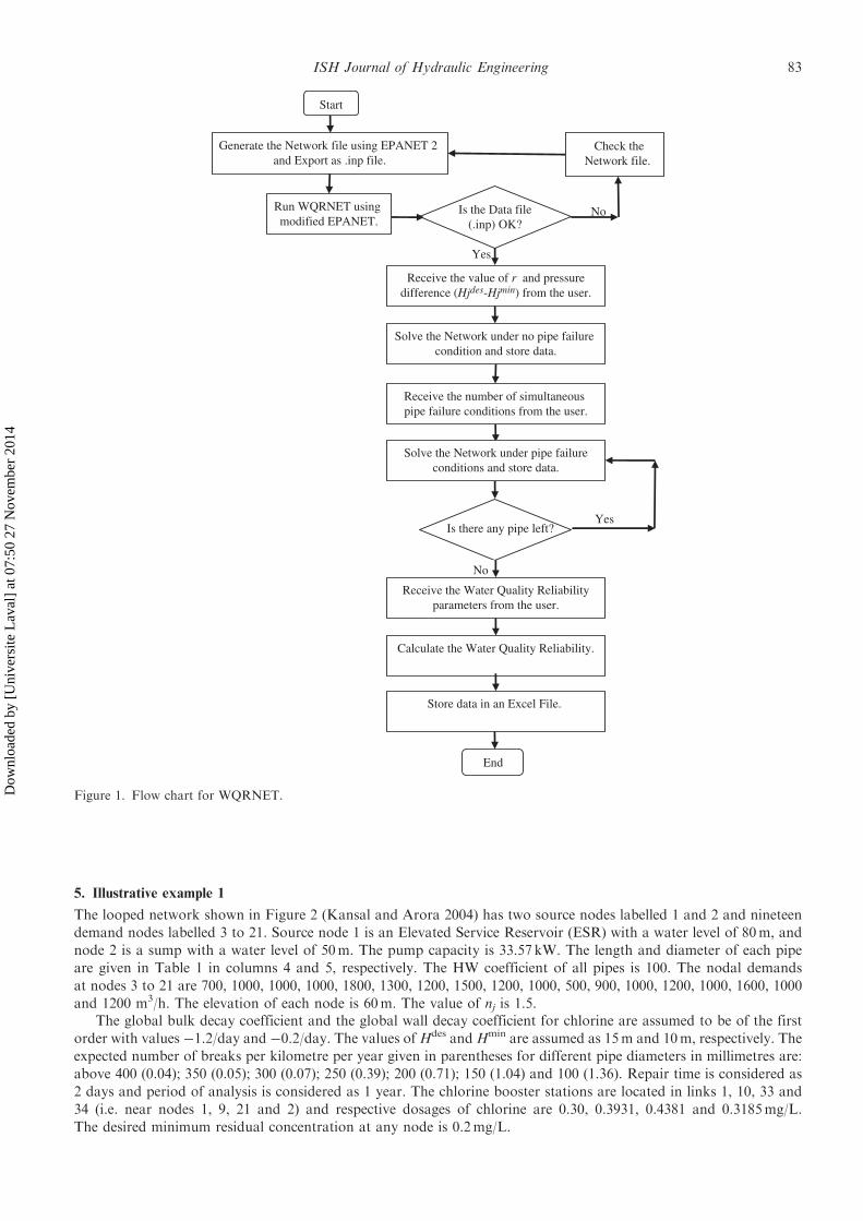
Steps for evaluating water quality reliability using WQRNET the for pipe-failure condition are as listed below, andin addition the procedure is shown using a flow-chart given in Figure 1.

Step 1 Considering all-pipes-working condition data file (a .net file) is generated (using EPANET 2 graphical userenvironment). The data file then exported as a .inp file to be used as an input file, which in turn will be solved bymodified EPANET.

Step 2 The programme WQRNET then runs, which in turn calls modified EPANET to solve the network (the .inpfile). At first the network is solved for no-pipe-failure condition and the result is stored for further use.

Step 3 Now, the network is solved for the pipe-failure condition. Pipe number(s) under the failure condition issupplied by the user during run time. WQRNET can solve single- or multiple-pipe-failure conditions at a time. In thiscase, WQRNET solves the network for pipe 1 under the failure condition and available nodal flows and correspondingsteady-state chlorine concentrations at different nodes are stored for further use. The step is repeated for other pipe-failure conditions one by one.

Step 4 Based on the pipe failure data, closure and working time for that condition is obtained. In case of singleloading pattern, each condition becomes a state as the hydraulic conditions remains constant in that period.

Step 5 Considering the available nodal flows and available chlorine concentrations obtained in steps 2 and 3 alongwith time for different states obtained in step 4, water quality reliability is evaluated and stored in an Excel file.

82 R. Gupta et al.

Dow

nloa

ded

by [

Uni

vers

ite L

aval

] at

07:

50 2

7 N

ovem

ber

2014

5. Illustrative example 1

The looped network shown in Figure 2 (Kansal and Arora 2004) has two source nodes labelled 1 and 2 and nineteen

demand nodes labelled 3 to 21. Source node 1 is an Elevated Service Reservoir (ESR) with a water level of 80m, and

node 2 is a sump with a water level of 50m. The pump capacity is 33.57 kW. The length and diameter of each pipe

are given in Table 1 in columns 4 and 5, respectively. The HW coefficient of all pipes is 100. The nodal demands

at nodes 3 to 21 are 700, 1000, 1000, 1000, 1800, 1300, 1200, 1500, 1200, 1000, 500, 900, 1000, 1200, 1000, 1600, 1000

and 1200 m3/h. The elevation of each node is 60m. The value of nj is 1.5.The global bulk decay coefficient and the global wall decay coefficient for chlorine are assumed to be of the first

order with values �1.2/day and �0.2/day. The values ofHdes andHmin are assumed as 15m and 10m, respectively. The

expected number of breaks per kilometre per year given in parentheses for different pipe diameters in millimetres are:

above 400 (0.04); 350 (0.05); 300 (0.07); 250 (0.39); 200 (0.71); 150 (1.04) and 100 (1.36). Repair time is considered as

2 days and period of analysis is considered as 1 year. The chlorine booster stations are located in links 1, 10, 33 and

34 (i.e. near nodes 1, 9, 21 and 2) and respective dosages of chlorine are 0.30, 0.3931, 0.4381 and 0.3185mg/L.

The desired minimum residual concentration at any node is 0.2mg/L.

Yes

No

Yes

Start

Generate the Network file using EPANET 2 and Export as .inp file.

Run WQRNET using modified EPANET.

Receive the value of r and pressuredifference (Hjdes-Hjmin) from the user.

Is the Data file(.inp) OK?

Solve the Network under no pipe failure condition and store data.

Check theNetwork file.

Receive the number of simultaneous pipe failure conditions from the user.

Solve the Network under pipe failureconditions and store data.

Is there any pipe left?

No

Receive the Water Quality Reliabilityparameters from the user.

Calculate the Water Quality Reliability.

Store data in an Excel File.

End

Figure 1. Flow chart for WQRNET.

ISH Journal of Hydraulic Engineering 83

Dow

nloa

ded

by [

Uni

vers

ite L

aval

] at

07:

50 2

7 N

ovem

ber

2014

5.1. Performance of the network under normal and pipe-failure conditions

NFA of WDN (Gupta and Bhave 1996 a) is carried out under no-pipe-failure and a single-pipe-failure condition.

Herein, the modified EPANET is for NFA (Ganguly 2007). Available flows and available chlorine concentration at

various nodes for no pipe failure and few single-pipe-failure conditions obtained using the proposed methodology are

also given in Tables 2 and 3, respectively. It can be observed from Table 2 that because all the demand nodes are at the

same elevation, they are receiving at least some part of the demand. There are no no-flow nodes. Kansal’s hydraulic

model (Kansal and Arora 2004) wrongly predicted many nodes as no-flow nodes. Thus, herein the hydraulic behaviour

of network under pressure-deficient condition is properly considered while estimating the available residual chlorine

concentrations. Further, it can be observed from Table 3 that there are few nodes where the residual chlorine

concentration is less than the desired concentration of 0.2mg/L. Such values are shown by bold-faced letters. This can

be observed even during the normal working condition.

OHSR

1

3

7 6

5 4

8

10 11

9

12 13

17 16 18

21 19 20

15

14

Pump

(3)

)7( )5(

(9) (10)

(13)

(19)(18)(17)(16)

(1) (2)

)6( )4(

(8)

)51( )21( )11( (14)

(20) (21) (22) (23) (24)

(25) (26)

(31)(30)(29)(28)

(27)

(32) (33)

(34)

Sump

2

Figure 2. A water distribution network as an illustrative example.

Table 1. Pipe data for the illustrative network shown in Figure 1.

Pipe Head Tail Length Diameter Availability Pipe Head Tail Length Diameter Availabilityno. node node (m) (mm) no. node node (m) (mm)(1) (2) (3) (4) (5) (6) (1) (2) (3) (4) (5) (6)

1 1 3 600 400 0.9999 18 13 12 900 250 0.99812 3 4 900 350 0.9998 19 14 13 900 350 0.99983 4 5 900 300 0.9997 20 10 15 900 300 0.99974 3 6 900 350 0.9998 21 11 16 900 250 0.99815 4 7 900 350 0.9998 22 12 17 900 250 0.99816 5 8 900 300 0.9997 23 13 17 1272 250 0.99737 5 9 1272 200 0.9951 24 13 18 900 300 0.99978 6 7 900 250 0.9981 25 15 16 900 250 0.99819 7 8 900 250 0.9981 26 17 16 900 200 0.996510 9 8 900 200 0.9965 27 18 17 900 250 0.998111 6 10 900 300 0.9997 28 15 19 900 200 0.996512 6 11 1272 250 0.9973 29 16 20 900 200 0.996513 7 11 900 250 0.9981 30 16 21 1272 200 0.995114 8 12 900 250 0.9981 31 17 21 900 200 0.996515 13 9 900 200 0.9965 32 20 19 900 200 0.996516 11 10 900 250 0.9981 33 21 20 900 200 0.996517 12 11 900 250 0.9981 34 2 14 600 400 0.9999

84 R. Gupta et al.

Dow

nloa

ded

by [

Uni

vers

ite L

aval

] at

07:

50 2

7 N

ovem

ber

2014

5.2. Reliability analysis

For calculating reliability parameters, time for different states is required. It depends on the value of pipe availability(ratio of working time to total time) and non-availability (ratio of failure time to total time) of pipe. In order to obtainthese values, we have to calculate failure probability, closure time and working time. For example, for pipe 1, thefailure probability is 0.024 breaks per year (0.04 breaks/km/year� 0.6 km, the length of the pipe), closure time per yearis 0.048 days (0.024 breaks/year� 2 days, the repair time), working time per year is 364.952 days (365 – 0.048¼ 364.952days, period of analysis), pipe availability, is 364.952� 365¼ 0.99986 and pipe non-availability, is 0.00014(1 – 0.99986). Probability of pipe working (i.e. availability) is given in Table 1.

The states with same number of shutdown pipes are grouped together to obtain the time duration for each stategroup. Two state groups 1 and 2 are considered as given in Table 4. State group 1 consists of all-pipes-workingcondition, and therefore there is only one state. The state group 2 consists of one-pipe-failure condition and thereforethere are 34 states, one for each pipe failure condition. The probability of simultaneous failure of two or more pipes isvery less and ignored. Total time for state group is sum of time of each state in that group. The time for different statesis obtained by considering the availability and unavailability of pipe. For example, for state 1 in which all pipes inworking condition is the product of availability of each pipe multiplied with 365 and is obtained as 341.15 days. Also,the time for state group becomes 341.15 days (column 2, Table 4). For state corresponding to pipe 1 failed condition,time for the state will be product of unavailability of pipe 1 with availability of other pipes multiplied by 365 and is0.04487 days. Similarly, the time for other states is obtained. Total time for state group 2 (one-pipe-failure condition) isobtained as 23.09 days. Thus, the cumulative time for these two state groups is 364.24 days out of 365 days (column 3,Table 4). Now, using the available flows, available residual concentration and time for the different states, both volumereliability (Rv) (Gupta and Bhave 1996 a) and water quality reliability parameters of the network are obtained as givenin Table 4 in columns 4 and 5, respectively.

Difference in Rv and RWQ provides an assessment of the quantity of water supplied without meeting the desiredwater quality criteria. The water quality reliability can be improved by providing additional chlorination station or byadjusting the chlorine dose.

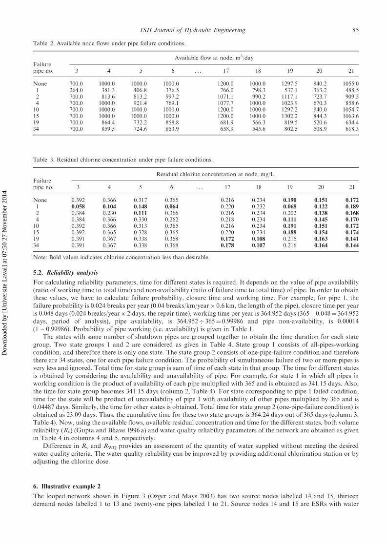
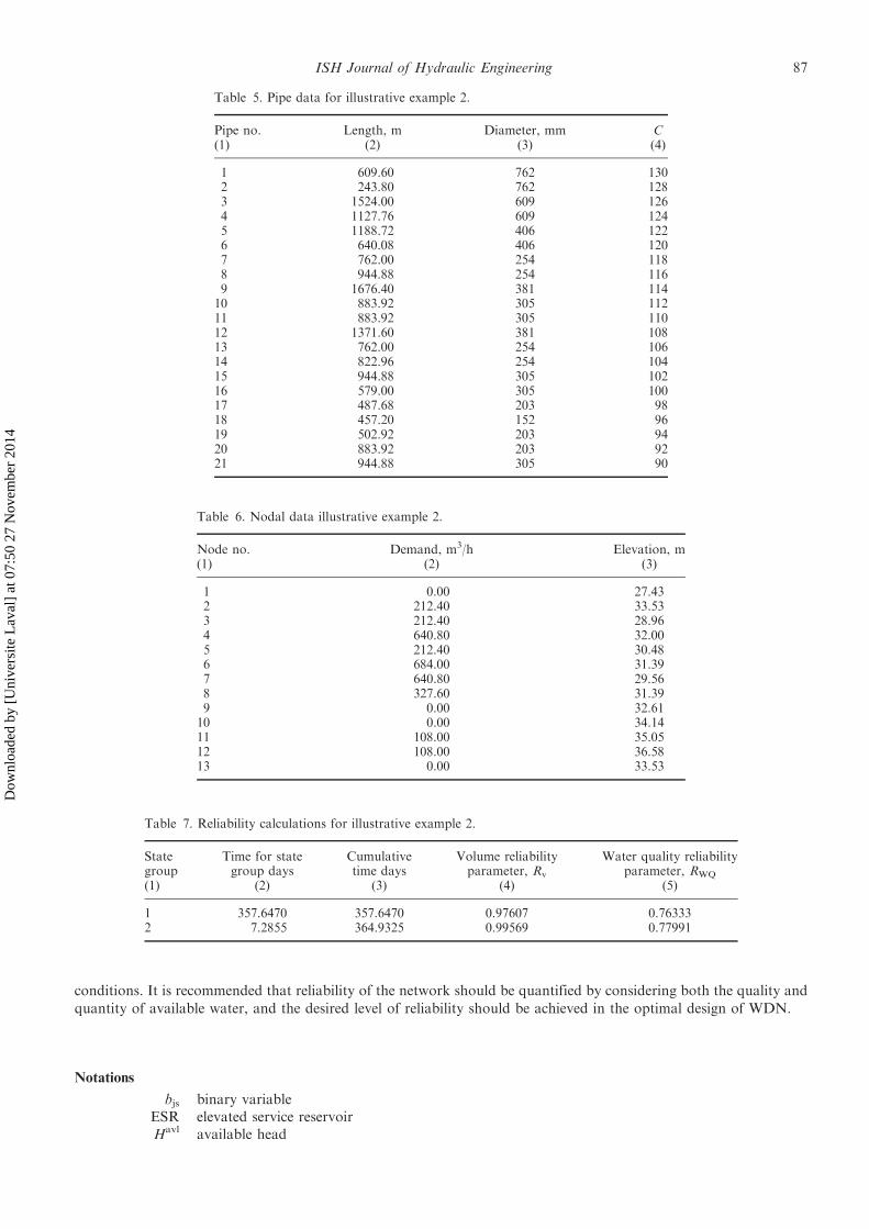
6. Illustrative example 2

The looped network shown in Figure 3 (Ozger and Mays 2003) has two source nodes labelled 14 and 15, thirteendemand nodes labelled 1 to 13 and twenty-one pipes labelled 1 to 21. Source nodes 14 and 15 are ESRs with water

Table 3. Residual chlorine concentration under pipe failure conditions.

Failurepipe no.

Residual chlorine concentration at node, mg/L

3 4 5 6 . . . 17 18 19 20 21

None 0.392 0.366 0.317 0.365 0.216 0.234 0.190 0.151 0.172

1 0.058 0.104 0.148 0.064 0.220 0.232 0.068 0.122 0.189

2 0.384 0.230 0.111 0.366 0.216 0.234 0.202 0.138 0.1684 0.384 0.366 0.330 0.262 0.218 0.234 0.111 0.145 0.170

10 0.392 0.366 0.313 0.365 0.216 0.234 0.191 0.151 0.172

15 0.392 0.365 0.328 0.365 0.220 0.234 0.188 0.154 0.17419 0.391 0.367 0.338 0.368 0.172 0.108 0.215 0.163 0.141

34 0.391 0.367 0.338 0.368 0.178 0.107 0.216 0.164 0.144

Note: Bold values indicates chlorine concentration less than desirable.

Table 2. Available node flows under pipe failure conditions.

Failurepipe no.

Available flow at node, m3/day

3 4 5 6 . . . 17 18 19 20 21

None 700.0 1000.0 1000.0 1000.0 1200.0 1000.0 1297.5 840.2 1055.01 264.0 381.3 406.8 376.5 766.0 798.3 537.1 363.2 488.52 700.0 813.6 813.2 997.2 1071.1 990.2 1117.1 723.7 909.54 700.0 1000.0 921.4 769.1 1077.7 1000.0 1023.9 670.3 858.610 700.0 1000.0 1000.0 1000.0 1200.0 1000.0 1297.2 840.0 1054.715 700.0 1000.0 1000.0 1000.0 1200.0 1000.0 1302.2 844.3 1063.619 700.0 864.4 732.2 858.8 681.9 566.3 819.5 520.6 634.434 700.0 859.5 724.6 853.9 658.9 545.6 802.5 508.9 618.3

ISH Journal of Hydraulic Engineering 85

Dow

nloa

ded

by [

Uni

vers

ite L

aval

] at

07:

50 2

7 N

ovem

ber

2014

levels of 60.96m. Length, diameter and Hazen-Williams constant (C) of each pipe are given in Table 5. The global bulkdecay coefficient and global wall decay coefficient for chlorine are assumed to be of first order with values as –1.2/dayand –0.2/day. Nodal demands and elevations are given in Table 6. Herein, the minimum required HGL value at a nodeis considered as its elevation and the desirable pressure at a node is 15m above minimum HGL. Demand nodes 1, 9, 10and 13 have no demand. The data for expected number of breaks per kilometre per year is same as used in the previousexample. Repair time is considered as 2 days and period of analysis is considered as 1 year. Four booster stations atnodes 8, 12, 14 and 15 are considered having chlorine concentrations of 0.2, 0.2, 0.2302 and 0.2282mg/L, respectively.

6.1. Solution

NFA is carried out in order to obtain available nodal flows and available chlorine concentrations for the all-pipe-working and one-pipe-failure conditions. By using nodal flow values, the volume reliability and water quality reliabilityare calculated. The obtained reliability parameters are shown in Table 7. It can be observed from Table 7 that thevolume reliability parameter of the network is 0.99569, whereas the water quality reliability parameter is 0.77991.It shows that during some periods, the network is not able to satisfy the required quality criteria while meeting thedemands fully or partially.

7. Summary and conclusions

A new water quality reliability parameter is proposed for assessing the reliability of WDNs. This parameter has aphysical meaning, and this single parameter accounts for both the quality and quantity of water available at differentnodes of a WDN. A methodology based on the performance of WDN under the pressure-deficient condition issuggested for use in evaluation of water quality reliability. The method is illustrated with two example networks takenfrom the literature. Hydraulic and water quality reliability of example networks are compared, and it is observed thatat some of the nodes during some states, water of desired quality is not delivered. Water quality reliability assessment isuseful in determining the need for additional chlorination stations and modifying chlorine dose during pipe failure

ESR 2

ESR 1

19

1

2 3 4

5

789

1510 11

21

12

16 20

18

17

6

1314

9

1 42

567

3

810

11

13

12

14

15

Figure 3. Looped network of illustrative example 2.

Table 4. Volume and water quality reliability parameters.

Stategroup

Time for stategroup, days

Cumulativetime, days

Volume reliabilityparameter, Rv

Water quality reliabilityparameter, RWQ

(1) (2) (3) (4) (5)

1 341.15 341.15 0.89598 0.698342 23.09 364.24 0.95610 0.74609

86 R. Gupta et al.

Dow

nloa

ded

by [

Uni

vers

ite L

aval

] at

07:

50 2

7 N

ovem

ber

2014

conditions. It is recommended that reliability of the network should be quantified by considering both the quality and

quantity of available water, and the desired level of reliability should be achieved in the optimal design of WDN.

Notations

bjs binary variableESR elevated service reservoirHavl available head

Table 5. Pipe data for illustrative example 2.

Pipe no. Length, m Diameter, mm C(1) (2) (3) (4)

1 609.60 762 1302 243.80 762 1283 1524.00 609 1264 1127.76 609 1245 1188.72 406 1226 640.08 406 1207 762.00 254 1188 944.88 254 1169 1676.40 381 11410 883.92 305 11211 883.92 305 11012 1371.60 381 10813 762.00 254 10614 822.96 254 10415 944.88 305 10216 579.00 305 10017 487.68 203 9818 457.20 152 9619 502.92 203 9420 883.92 203 9221 944.88 305 90

Table 6. Nodal data illustrative example 2.

Node no. Demand, m3/h Elevation, m(1) (2) (3)

1 0.00 27.432 212.40 33.533 212.40 28.964 640.80 32.005 212.40 30.486 684.00 31.397 640.80 29.568 327.60 31.399 0.00 32.6110 0.00 34.1411 108.00 35.0512 108.00 36.5813 0.00 33.53

Table 7. Reliability calculations for illustrative example 2.

Stategroup

Time for stategroup days

Cumulativetime days

Volume reliabilityparameter, Rv

Water quality reliabilityparameter, RWQ

(1) (2) (3) (4) (5)

1 357.6470 357.6470 0.97607 0.763332 7.2855 364.9325 0.99569 0.77991

ISH Journal of Hydraulic Engineering 87

Dow

nloa

ded

by [

Uni

vers

ite L

aval

] at

07:

50 2

7 N

ovem

ber

2014

Hmin minimum required headHdes desirable head

L length of pipeN(y) pipe break rate in year yNFA node flow analysis

NHFR node head-flow relationshippð yÞ working-condition probability in year y�pð yÞ shutdown probability of a pipe in year yqavls available discharge rate during state sqreqs required discharge rate during state sRv volume reliability parameter

RWQ water quality reliability parameterTr time for closurets time for the state s

WDN water distribution network

Acknowledgements

The financial support received from the University Grants Commission for the research work is gratefullyacknowledged.

References

Agrawal, M.L., Gupta, R., and Bhave, P.R. (2007). ‘‘Optimal design of level 1 redundant water distribution systems considering

nodal storage.’’ J. Environ. Eng., 133(3), 319–330.Al-Zaharani, M., and Syed, J.A. (2004). ‘‘Hydraulic reliability analysis of water distribution systems.’’ J. Inst. Eng., Singapore, 1(1),

76–92.Awumah, K., Goulter, I., and Bhatt, S. (1991). ‘‘Entropy based redundancy measures in water distribution network design.’’

J. Hydraul. Eng., 117(5), 595–614.Bhave, P.R. (1981). ‘‘Node flow analysis of water distribution systems.’’ J. Trans. Eng., 107(4), 457–467.Bhave, P.R. (2003). Optimal design of water distribution networks, Alpha Science International Ltd., Oxford, United Kingdom;

Narosa Publishing House, New Delhi, India.Bhave, P.R., and Gupta, R. (2006). Analysis of water distribution networks, Alpha Science International Ltd., Oxford, United

Kingdom; Narosa Publishing House, New Delhi, India.

Boccelli, D.L., Tryby, M.E., Uber, J.H., Rossman, L.A., Zeirolf, M.L., and Polycarpou, M.M. (1998). ‘‘Optimal scheduling of

booster disinfection in water distribution systems.’’ J. Water Resour. Plan. Manage., 124(2), 99–111.Bouchart, F., and Goulter, I.C. (1991). ‘‘Reliability improvement in design of water distribution network recognizing valve

location.’’ Water Resour. Res., 27(12), 3029–3040.Boulos, P.F., Altman, T., Jarrige, P., and Collevati, F. (1995). ‘‘Discrete simulation approach for network-water-quality models.’’

J. Water Resour. Plan. Manage., 121(1), 49–60.Chandapillai, J. (1991). ‘‘Realistic simulation of water distribution systems.’’ J. Trans. Eng., 117(2), 258–263.Cullinane, M.J., Lansey, K.E., and Mays, L.W. (1992). ‘‘Optimization-availability-based design of water distribution networks.’’

J. Hydraul. Eng., 118(3), 420–441.Devi Prasad, T., and Park, N.S. (2004). ‘‘Multiobjective genetic algorithms for design of water distribution networks.’’ J. Water

Resour. Plan. Manage., 130(1), 73–82.

Fujiwara, O., and De Silva, A.U. (1990). ‘‘Algorithm for reliability based optimal design of water networks.’’ J. Environ. Eng.,

116(3), 575–587.Fujiwara, O., and Ganesharajah, T. (1993). ‘‘Reliability assessment of water supply systems with storage and distribution

networks.’’ Water Resour. Res., 29(8), 2917–2924.Ganguly, S. (2007). ‘‘Node flow analysis of water distribution networks using EPANET 2.’’ M.Tech. thesis, Visvesvaraya National

Institute of Technology, Nagpur, India.Germanopoulos, G. (1985). ‘‘A technical note on the inclusion of pressure-dependent demand and leakage term in water supply

network models.’’ Civ. Eng. Systems, 2(3), 171–179.

Goulter, I., and Bouchart, F. (1990). ‘‘Reliability constrained pipe network model.’’ J. Hydraul. Eng., 116(2), 211–229.Goulter, I.C., and Coals, A.V. (1986). ‘‘Quantitative approaches to reliability assessment in pipe networks.’’ J. Trans. Eng., 112(3),

287–301.

Guercio, R., and Xu, Z. (1997). ‘‘Linearized optimization model for reliability-based design of water systems.’’ J. Hydraul. Eng.,

123(11), 1020–1026.

Gupta, R., and Bhave, P.R. (1994). ‘‘Reliability analysis of water distribution systems.’’ J. Environ. Eng., 120(2), 447–460.Gupta, R., and Bhave, P.R. (1996a). ‘‘Reliability based design of water distribution systems.’’ J. Environ. Eng., 122(1), 51–54.

88 R. Gupta et al.

Dow

nloa

ded

by [

Uni

vers

ite L

aval

] at

07:

50 2

7 N

ovem

ber

2014

Gupta, R., and Bhave, P.R. (1996b). ‘‘Comparison of methods for predicting deficient network performance.’’ J. Water Resour.

Plan. Manage., 122(3), 214–217.Gupta, R., Dhapade, S., Agrawal, M.L., and Bhave, P.R. (2007). ‘‘Modeling water quality in distribution network for reliability

analysis.’’ Proc. Natl. Workshop on Water Quality Problems and Mitigation through Sustainable Sources, Indian Water WorksAssoc., Raipur Centre, Chhattisgarh, India.

Kalungi, P., and Tanyimboh, T.T. (2003). ‘‘Redundancy model for water distribution systems.’’ Reliab. Eng. Syst. Saf., 82, 275–286.Kang, D., and Lansey, A.M. (2010). ‘‘Real time optimal valve operation and booster disinfection in water distribution systems.’’

J. Water Resour. Plan. Manage., 136(4), 463–473.

Kansal, M.L., and Arora, G. (2004). ‘‘Water quality reliability analysis in an urban distribution network.’’ J. Indian Water WorksAssoc., 36(3), 185–198.

Kessler, A., Ormsbee, L.E., and Shamir, U. (1990). ‘‘A methodology for least cost design of invulnerable water distribution

networks.’’ Civ. Eng. Syst., 7(1), 20–28.Kettler, A.J., and Goulter, I.C. (1985). ‘‘An analysis of pipe breakage in urban water distribution networks.’’ Can. J. Civ. Eng.,

12(2), 286–293.

Morgan, D.R., and Goulter, I.C. (1985). ‘‘Optimal urban water distribution design.’’ Water Resour. Res., 21(5), 642–652.Munavalli, G.R., and Mohan Kumar, M.S. (2003). ‘‘Optimal scheduling of multiple chlorine sources in water distribution systems.’’

J. Water Resour. Plan. Manage., 129(6), 493–504.Park, H., and Liebman, J.C. (1993). ‘‘Reliability-constrained minimum-cost design of water distribution nets.’’ J. Water Resour.

Plan. Manage., 119(1), 83–88.Ormsbee, L., and Kessler, A. (1990). ‘‘Optimal upgrading of hydraulic-network reliability.’’ J. Water Resour. Plan. Manage., 116(6),

784–802.

Ostfeld, A. (2004). ‘‘Reliability analysis of water distribution systems.’’ J. Hydroinform., 6(4), 281–294.Ostfeld, A., and Salomons, E. (2006). ‘‘Conjunctive optimal scheduling of pumping and booster chlorine injections in water

distribution systems.’’ Eng. Optim., 38(3), 337–352.

Ozger, S.S., and Mays, L.W. (2003). ‘‘A semi-pressure-driven approach to reliability assessment of water distribution networks.’’Proc. 30th IAHR Congress, Thessaloniki, Greece, 345-352.

Prasad, T.D., Walters, G.A., and Savic, D.A. (2004). ‘‘Booster disinfection of water supply networks: Multiobjective approach.’’J. Water Resour. Plan. Manage., 130(5), 367–376.

Rossman, L.A. (2001). EPANET User’s Manual, Risk Reduction Eng. Lab., USEPA, EPA, Cincinnati, OH.Rossman, L.A., Clark, R.M., and Grayman, W.M. (1994). ‘‘Modeling chlorine residuals in drinking water distribution systems.’’

J. Environ. Eng., 120(4), 803–821.

Rowell, W.F., and Barnes, W.J. (1982). ‘‘Optimal layout of water distribution systems.’’ J. Hydraul. Div., 108(1), 137–148.Su, Y.C., Mays, L.W., Duan, N., and Lansey, K.E. (1987). ‘‘Reliability-based optimization model for water distribution systems.’’

J. Hydraul. Eng., 114(12), 1539–1556.

Tanyimboh, T.T., and Templeman, A.B. (1993). ‘‘Optimal design of flexible water distribution networks.’’ Civ. Eng. Syst., 10(4),243–258.

Tolson, B.A., Maier, H.R., Simpson, A.R., and Lence, B.J. (2004). ‘‘Genetic algorithm for reliability-based optimization of water

distribution systems.’’ J. Water Resour. Plan. Manage., 130(1), 63–72.Tryby, M.E., Boceelli, D.L., Uber, J.G., and Rossman, L.A. (2002). ‘‘Facility location model for booster disinfection of water

supply networks.’’ J. Water Resour. Plan. Manage., 128(5), 322–333.Wagner, J., Shamir, U., and Marks, D. (1988). ‘‘Water distribution system reliability: simulation methods.’’ J. Water Resour. Plan.

Manage., 114(3), 276–293.Xu, C., and Goulter, I.C. (1998). ‘‘Probabilistic model for water distribution reliability.’’ J. Water Resour. Plan. Manage., 124(4),

218–228.

ISH Journal of Hydraulic Engineering 89

Dow

nloa

ded

by [

Uni

vers

ite L

aval

] at

07:

50 2

7 N

ovem

ber

2014